


Interfaces
of HEIDENHAIN Encoders
July 2013

Interfaces
As defined transitions between encoders and subsequent electronics, interfaces ensure the reliable exchange of information.
HEIDENHAIN offers encoders with interfaces for many common subsequent electronics.The interface possible in each respective case depends, among other things, on the measuring method used by the encoder.
Measuring methods
In the incremental measuring method the position information is obtained by counting the individual increments (measuring steps) from some point of origin. Since an absolute reference is necessary in order to determine the positions, a reference-mark signal is output as well. As a general rule, encoders that operate with the incremental measuring method output incremental signals.
Some incremental encoders with integrated interface electronics also have a counting function: Once the reference mark is traversed, an absolute position value is formed and output via a serial interface.
Note
Specialized encoders can have other interface properties, such as regarding the shielding.
With the absolute measuring method the absolute position information is gained directly from the graduation of the measuring standard.The position value is available from the encoder immediately upon switch-on and can be called at any time by the subsequent electronics.
Encoders that operate with the absolute measuring method output position values. Some interfaces provide incremental signals as well.
Absolute encoders do not require a reference run, which is advantageous particularly in concatenated manufacturing systems, transfer lines, or machines with numerous axes. Also, they are more resistant to EMC interferences.
Interface electronics
Interface electronics from HEIDENHAIN adapt the encoder signals to the interface of the subsequent electronics.They are used when the subsequent electronics cannot directly process the output signals from HEIDENHAIN encoders, or if additional interpolation of the signals is necessary.
You can find more detailed information in the Interface Electronics Product Overview.
This catalog supersedes all previous editions, which thereby become invalid. The basis for ordering from HEIDENHAIN is always the catalog edition valid when the contract is made.
2

Contents
Incremental signals
Sinusoidal signals |
1VPP |
Voltage signals, can be highly interpolated |
|
11 µAPP |
Current signals, can be interpolated |
Square-wave signals |
TTL |
RS 422, typically 5 V |
|
HTL |
Typically 10 V to 30 V |
|
|
|
|
HTLs |
Typically 10 V to 30 V, without inverted signals |
Position values
4
6
7
10
Serial interfaces |
EnDat |
Bidirectional interface |
With incremental signals |
12 |
|
|
|
|
|
|
|
|
Without incremental signals |
|
|
|
|
|
|
|
Siemens |
Company-specific information |
Without incremental signals |
15 |
|
|
|
|
|
|
Fanuc |
Company-specific information |
Without incremental signals |
|
|
|
|
|
|
|
Mitsubishi |
Company-specific information |
Without incremental signals |
|
|
|
|
|
|
|
PROFIBUS-DP |
Fieldbus |
Without incremental signals |
16 |
|
|
|
|
|
|
PROFINET IO |
Ethernet-based fieldbus |
Without incremental signals |
18 |
|
|
|
|
|
|
SSI |
Synchronous serial interface |
With incremental signals |
20 |
Other signals
Limit/Homing |
Limit switches |
With incremental signals |
|
Position detection |
With incremental signals |
Commutation signals |
Block commutation |
With incremental signals |
|
Sinusoidal commutation |
With incremental signals |
Further information
Overview of interface electronics
HEIDENHAIN testing equipment
General electrical information
22
23
24
25
26
28
32
3
Incremental signals
» 1 VPP sinusoidal signals
HEIDENHAIN encoders with » 1 VPP interface provide voltage signals that can be highly interpolated.
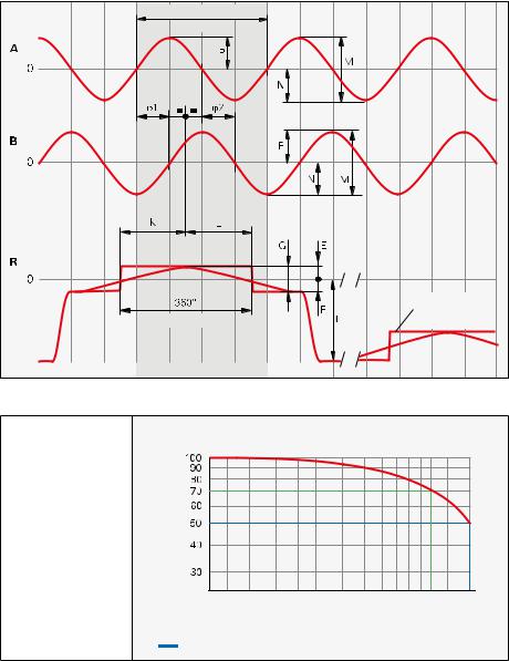
The sinusoidal incremental signals A and B are phase-shifted by 90° elec. and have an amplitude of typically 1 VPP.The illustrated sequence of output signals— with B lagging A—applies for the direction of motion shown in the dimension drawing.
The reference mark signal R has a usable component G of approx. 0.5 V. Next to the reference mark, the output signal can be reduced by up to 1.7 V to a quiescent level H.This must not cause the subsequent electronics to overdrive. Even at the lowered signal level, signal peaks with the amplitude G can also appear.
The data on signal amplitude apply when the supply voltage given in the specifications is connected to the encoder.They refer to a differential measurement at the 120 ohm terminating resistor between the associated outputs.The signal amplitude decreases with increasing frequency.The cutoff frequency indicates the scanning frequency at which a certain percentage of the original signal amplitude is maintained:
•–3 dB 70 % of the signal amplitude
•–6 dB 50 % of the signal amplitude
The data in the signal description apply to motions at up to 20 % of the –3 dB cutoff frequency.
Interpolation/resolution/measuring step
The output signals of the 1 VPP interface are usually interpolated in the subsequent electronics in order to attain sufficiently high resolutions. For velocity control, interpolation factors are commonly over 1000 in order to receive usable information even at low rotational or linear velocities.
Measuring steps for position measurement are recommended in the specifications. For special applications, other resolutions are also possible.
Short-circuit stability
A temporary short circuit of one signal output to 0 V or UP (except encoders with UPmin = 3.6 V) does not cause encoder failure, but it is not a permissible operating condition.
Short circuit at |
20 °C |
125 °C |
|
|
|
One output |
< 3 min |
< 1 min |
|
|
|
All outputs |
< 20 s |
< 5 s |
|
|
|
Interface |
Sinusoidal voltage signals » 1VPP |
|
Incremental signals |
Two nearly sinusoidal signals A and B |
|
|
Signal amplitude M: |
0.6 to 1.2 VPP; typically 1 VPP |
|
Asymmetry |P – N|/2M: |
0.065 |
|
Amplitude ratio MA/MB: |
0.8 to 1.25 |
|
Phase angle |j1 + j2|/2: |
90° ± 10° elec. |
|
|
|
Reference mark |
One or several signal peaks R |
|
signal |
Usable component G: |
0.2 V |
|
Quiescent value H: |
1.7 V |
|
Switching threshold E, F: |
0.04 V to 0.68 V |
|
Zero crossovers K, L: |
180° ± 90° elec. |
|
|
|
Connecting cable |
Shielded HEIDENHAIN cable |
|
Cable length |
For example PUR [4(2 x 0.14 mm2) + (4 x 0.5 mm2)] |
|
Max. 150 m at 90 pF/m distributed capacitance |
||
Propagation time |
6 ns/m |
|
|
|
|
These values can be used for dimensioning of the subsequent electronics. Any limited tolerances in the encoders are listed in the specifications. For encoders without integral bearing, reduced tolerances are recommended for initial operation (see the mounting instructions).
Signal period |
|
360° elec. |
|
|
Alternative |
(rated value) |
signal shape |
|
|
A, B, R measured with oscilloscope in differential mode |
|
Cutoff frequency
Typical signal amplitude curve with respect to
the scanning frequency (depends on encoder) [%]
amplitudeSignal
Scanning frequency [kHz]
 –3 dB cutoff frequency –6 dB cutoff frequency
4

Monitoring of the incremental signals
The following sensitivity levels are recommended for monitoring the signal amplitude M:
Lower threshold: Upper threshold:
The height of the incremental signals can be monitored, for example by the length of the resulting position indicator:The oscilloscope shows the output signals A and B as a Lissajous figure in the XY graph. Ideal sinusoidal signals produce a circle with the diameter M. In this case the position indicator r shown corresponds to ½M.The formula is therefore
r = (A2+B2)
with the condition 0.3 V < 2r < 1.35 V.
Input circuitry of subsequent electronics
Dimensioning
Operational amplifier, e.g. MC 34074
Z0 = 120
R1 = 10 k and C1 = 100 pF R2 = 34.8 k and C2 = 10 pF
UB = ±15 V U1 approx. U0
–3 dB cutoff frequency of circuitry
Approx. 450 kHz
Approx. 50 kHz with |
C1 = 1000 pF |
and |
C2 = 82 pF |
The circuit variant for 50 kHz does reduce the bandwidth of the circuit, but in doing so it improves its noise immunity.
Circuit output signals
Ua = 3.48 VPP typically
Gain 3.48
Input circuitry of subsequent electronics for high signal frequencies
For encoders with high signal frequencies (e.g. LIP 281), a special input circuitry is required.
Dimensioning
Operational amplifier, e.g. AD 8138
Z0 = 120
R1 = 681 ; R2 = 1 k ; R3 = 464 C0 = 15 pF; C1 = 10 pF
+UB = 5 V; –UB = 0 V or –5 V
–3 dB cutoff frequency of circuitry
Approx. 10 MHz
Circuit output signals
Ua = 1.47 VPP typically
Gain 1.47
|
Incremental signal A |
|
|
Time [t] |
Incremental signal B |
|
|
|
|
|
Time [t] |
Incremental signals |
|
|
Reference mark signal |
Encoder |
Subsequent electronics |
|
||
Ra < 100 , |
|
|
typically 24 |
|
|
Ca < 50 pF |
|
|
SIa < 1 mA |
|
|
U0 = 2.5 V ± 0.5 V |
|
|
(relative to 0 V of the |
|
|
supply voltage) |
|
|
Incremental signals |
|
|
Reference mark signal |
LIP 281 encoder |
Subsequent electronics |
|
Ra < 100 , typically 24
Ca < 50 pF SIa < 1 mA
U0 = 2.5 V ± 0.5 V (relative to 0 V of the
supply voltage)
5

Incremental signals
11 µAPP sinusoidal signals
HEIDENHAIN encoders with » 11 µAPP interface provide current signals.They
are intended for connection to ND position display units or EXE pulse-shaping electronics from HEIDENHAIN.
The sinusoidal incremental signals I1 and I2 are phase-shifted by 90° elec. and have signal levels of approx. 11 µAPP. The illustrated sequence of output signals—with I2 lagging I1—applies to the direction of motion shown in the dimension drawing, and for retracting plungers of length gauges.
The reference mark signal I0 has a usable component G of approx. 5.5 µA.
The data on signal amplitude apply when the supply voltage given in the Specifications is connected at the encoder.They refer to a differential measurement between the associated outputs.The signal amplitude decreases with increasing frequency.The cutoff frequency indicates the scanning frequency at which a certain percentage of the original signal amplitude is maintained:
•–3 dB cutoff frequency: 70 % of the signal amplitude
•–6 dB cutoff frequency: 50 % of the signal amplitude
Interpolation/resolution/measuring step
The output signals of the 11 µAPP interface are usually interpolated in the subsequent electronics—ND position displays or EXE pulse-shaping electronics from HEIDENHAIN— in order to attain sufficiently high resolutions.
Interface |
Sinusoidal current signals » 11 µAPP |
|
Incremental signals |
Two nearly sinusoidal signals I1 and I2 |
|
|
Signal amplitude M: |
7 to 16 µAPP/typically 11 µAPP |
|
Asymmetry IP – NI/2M: |
0.065 |
|
Amplitude ratio MA/MB: |
0.8 to 1.25 |
|
Phase angle |j1 + j2|/2: |
90° ± 10° elec. |
|
|
|
Reference mark |
One or more signal peaks I0 |
|
signal |
Usable component G: |
2 µA to 8.5 µA |
|
Switching threshold E, F: |
0.4 µA |
|
Zero crossovers K, L: |
180° ± 90° elec. |
Connecting cable |
Shielded HEIDENHAIN cable |
Cable length |
PUR [3(2 · 0.14 mm2) + (2 · 1 mm2)] |
Max. 30 m with 90 pF/m distributed capacitance |
|
Propagation time |
6 ns/m |
|
Signal period |
|
360° elec. |
|
(rated value) |
6

TTL square-wave signals
HEIDENHAIN encoders with «TTL interface incorporate electronics that digitize sinusoidal scanning signals with or without interpolation.
The incremental signals are transmitted as the square-wave pulse trains Ua1 and Ua2, phase-shifted by 90° elec.The reference mark signal consists of one or more reference pulses Ua0, which are gated with the incremental signals. In addition, the integrated electronics produce their inverted signals ¢, £ and ¤ for noise-proof transmission.The illustrated sequence of output signals—with Ua2 lagging Ua1—applies to the direction of motion shown in the dimension drawing.
The fault-detection signal ¥ indicates fault conditions such as breakage of the power line or failure of the light source. It can be used for such purposes as machine shut-off during automated production.
The distance between two successive edges of the incremental signals Ua1 and Ua2 through 1-fold, 2-fold or 4-fold evaluation is one measuring step.
The subsequent electronics must be designed to detect each edge of the square-wave pulse.The minimum edge separation a stated in the Specifications applies for the specified input circuit with a cable length of 1 m and refers to a measurement at the output of the differential line receiver.
Note
Not all encoders output a reference mark signal, fault-detection signal, or their inverted signals. Please see the connector layout for this.
Interface |
Square-wave signals «TTL |
|
|
|
|
Incremental signals |
TwoTTL square-wave signals Ua1, Ua2 and their inverted |
|
|
signals ¢, £ |
|
|
|
|
Reference mark |
One or moreTTL square-wave pulses Ua0 and their inverted |
|
signal |
pulses ¤ |
|
Pulse width |
90° elec. (other widths available on request) |
|
Delay time |
|td| 50 ns |
|
Fault-detection |
OneTTL square-wave pulse ¥ |
|
signal |
Improper function: LOW (upon request: Ua1/Ua2 high impedance) |
|
Pulse width |
Proper function: HIGH |
|
tS 20 ms |
|
|
Signal amplitude |
Differential line driver as per EIA standard RS-422 |
|
|
|
|
Permissible load |
Z0 100 |
Between associated outputs |
|
|IL| 20 mA |
Max. load per output (ERN 1x23: 10 mA) |
|
Cload 1000 pF |
With respect to 0 V |
|
Outputs protected against short circuit to 0 V |
|
|
|
|
Switching times |
t+ / t– 30 ns (typically 10 ns) |
|
(10 % to 90 %) |
with 1 m cable and recommended input circuitry |
|
|
|
|
Connecting cable |
Shielded HEIDENHAIN cable |
|
Cable length |
For example PUR [4(2 × 0.14 mm2) + (4 × 0.5 mm2)] |
|
Max. 100 m (¥ max. 50 m) at distributed capacitance 90 pF/m |
||
Propagation time |
Typically 6 ns/m |
|
|
|
|
Signal period 360° elec. |
Fault |
Measuring step after |
|
4-fold evaluation |
|
Inverse signals ¢, £, ¤ are not shown
7

Clocked output signals are typical for encoders and interpolation electronics with 5-fold interpolation (or greater).They derive the edge separation a from an internal clock source. At the same time, the clock frequency determines the permissible input frequency of the incremental signals (1 VPP or 11 µAPP) and the resulting maximum permissible traversing velocity or shaft speed:
anom = |
1 |
|
|
|
4 · IPF · fenom |
|
|
anom |
nominal edge separation |
||
IPF |
interpolation factor |
||
fenom |
nominal input frequency |
||
The tolerances of the internal clock source have an influence on the edge separation a of the output signal and the input frequency fe, thereby influencing the traversing velocity or shaft speed.
The data for edge separation already takes these tolerances into account with 5 %: Not the nominal edge separation is indicated, but rather the minimum edge separation amin.
On the other hand, the maximum permissible input frequency must consider a tolerance of at least 5 %.This means that the maximum permissible traversing velocity or shaft speed are also reduced accordingly.
Encoders and interpolation electronics without interpolation in general do not have clocked output signals.The minimum edge separation amin that occurs at the maximum possible input frequency is stated in the specifications. If the input frequency is reduced, the edge separation increases correspondingly.
Cable-dependent differences in the propagation time additionally reduce the edge separation by 0.2 ns per meter of cable.To prevent counting errors, a safety margin of 10 % must be considered, and the subsequent electronics so designed that they can process as little as 90 % of the resulting edge separation.
Please note:
The max. permissible shaft speed or traversing velocity must never be exceeded, since this would result in an irreversible counting error.
Calculation example 1
LIDA 400 linear encoder
Requirements: display step 0.5 µm, traversing velocity 1 m/s, output signalsTTL, cable length to subsequent electronics 25 m.
What minimum edge separation must the subsequent electronics be able to process?
Selection of the interpolation factor |
|
20 µm grating period : 0.5 µm display step = |
40-fold subdivision |
Evaluation in the subsequent electronics |
4-fold |
Interpolation |
10-fold |
Selection of the edge separation
Traversing velocity |
60 m/min (corresponds to 1 m/s) |
+ tolerance value 5 % |
63 m/min |
Select in specifications: |
|
Next LIDA 400 version |
120 m/min (from specifications) |
Minimum edge separation |
0.22 µs (from specifications) |
Determining the edge separation that the subsequent electronics must process
Subtract cable-dependent differences in the propagation time |
0.2 ns per meter |
For cable length = 25 m |
5 ns |
Resulting edge separation |
0.215 µs |
Subtract 10 % safety margin |
0.022 µs |
Minimum edge separation for the subsequent electronics |
0.193 µs |
Calculation example 2
ERA 4000 angle encoder with 32 768 lines
Requirements: measuring step 0.1”, output signalsTTL (IBV external interface electronics necessary), cable length from IBV to subsequent electronics = 20 m, minimum edge separation that the subsequent electronics can process = 0.5 µs (input frequency = 2 MHz).
What rotational speed is possible?
Selection of the interpolation factor |
|
32 768 lines corresponds to |
40” signal period |
Signal period 40” : measuring step 0.1” = |
400-fold subdivision |
Evaluation in the subsequent electronics |
4-fold |
Interpolation in the IBV |
100-fold |
Calculation of the edge separation |
|
Permissible edge separation of the subsequent electronics |
0.5 µs |
This corresponds to 90 % of the resulting edge separation |
|
This leads to: Resulting edge separation |
0.556 µs |
Subtract cable-dependent differences in the propagation time |
0.2 ns per meter |
For cable length = 20 m |
4 ns |
Minimum edge separation of IBV 102 |
0.56 µs |
Selecting the input frequency
According to the Product Information, the input frequencies and therefore the edge
separations a of the IBV 102 can be set. |
|
Next suitable edge separation |
0.585 µs |
Input frequency at 100-fold interpolation |
4 kHz |
Calculating the permissible shaft speed |
|
Subtract 5 % tolerance |
3.8 kHz |
This is 3 800 signals per second or 228 000 signals per minute.
Meaning for 32 768 lines of the ERA 4000:
Max. permissible rotational speed |
6.95 rpm |
8

The permissible cable length for transmission of theTTL square-wave signals to the subsequent electronics depends on the edge separation a. It is at most 100 m, or 50 m for the fault detection signal.This requires, however, that the voltage supply (see Specifications) be ensured at the encoder.The sensor lines can be used to measure the voltage at the encoder and, if required, correct it with an automatic control system (remote sense voltage supply).
Greater cable lengths can be provided upon consultation with HEIDENHAIN.
Permissible cable length
with respect to the edge separation
|
Without ¥ |
|
length [m] |
With ¥ |
|
Cable |
||
|
Edge separation [µs]
Input circuitry of |
Incremental signals |
Encoder |
Subsequent electronics |
|
subsequent electronics |
Reference mark signal |
|
|
|
Dimensioning |
|
|
|
|
IC1 = Recommended differential line |
|
|
|
|
|
receiver |
|
|
|
|
DS 26 C 32 AT |
|
|
|
|
Only for a > 0.1 µs: |
Fault-detection signal |
|
|
|
AM 26 LS 32 |
|
|
|
|
|
|
|
|
|
MC 3486 |
|
|
|
|
SN 75 ALS 193 |
|
|
|
R1 |
= 4.7 k |
|
|
|
R2 |
= 1.8 k |
|
|
|
Z0 |
= 120 |
|
|
|
C1 |
= 220 pF (serves to improve noise |
|
|
|
|
immunity) |
|
|
|
9

Incremental signals
HTL square-wave signals
HEIDENHAIN encoders with « HTL interface incorporate electronics that digitize sinusoidal scanning signals with or without interpolation.
The incremental signals are transmitted as the square-wave pulse trains Ua1 and Ua2, phase-shifted by 90° elec.The reference mark signal consists of one or more reference pulses Ua0, which are gated with the incremental signals. In addition, the integrated electronics produce their inverted signals ¢, £ and ¤ for noise-proof transmission (does not apply to HTLs).
The illustrated sequence of output signals—with Ua2 lagging Ua1—applies to the direction of motion shown in the dimension drawing.
The fault-detection signal ¥ indicates fault conditions such as failure of the light source. It can be used for such purposes as machine shut-off during automated production.
The distance between two successive edges of the incremental signals Ua1 and Ua2 through 1-fold, 2-fold or 4-fold evaluation is one measuring step.
The subsequent electronics must be designed to detect each edge of the square-wave pulse.The minimum edge separation a listed in the Specifications refers to a measurement at the output of the given differential input circuitry.To prevent counting errors, the subsequent electronics should be designed so that they can process as little as 90% of the edge separation a.
The maximum permissible shaft speed or traversing velocity must never be exceeded.
Interface |
Square-wave signals « HTL, « HTLs |
|
|
Incremental signals |
Two HTL square-wave signals Ua1, Ua2 and their inverted |
signals ¢, £ (HTLs without ¢, £)
Reference mark signal |
One or more HTL square-wave pulses Ua0 and their |
||
Pulse width |
inverted pulses ¤ (HTLs without ¤) |
||
90° elec. (other widths available on request) |
|||
Delay time |
|td| 50 ns |
|
|
Fault-detection signal |
One HTL square-wave pulse ¥ |
||
|
Improper function: LOW |
|
|
|
Proper function: HIGH |
|
|
Pulse width |
tS 20 ms |
|
|
Signal levels |
UH 21 V at –IH = 20 mA |
With voltage supply of |
|
|
UL 2.8 V at IL = 20 mA |
UP = 24 V, without cable |
|
Permissible load |
|IL| 100 mA |
Max. load per output, (except ¥) |
|
|
Cload 10 nF |
With respect to 0 V |
|
|
Outputs short-circuit proof for max. 1 minute to 0 V and UP |
||
|
(except ¥) |
|
|
|
|
|
|
Switching times |
t+/t– 200 ns (except ¥) |
|
|
(10 % to 90 %) |
with 1 m cable and recommended input circuitry |
||
|
|
||
Connecting cable |
HEIDENHAIN cable with shielding |
||
Cable length |
e. g. PUR [4(2 × 0.14 mm2) + (4 × 0.5 mm2)] |
||
Max. 300 m (HTLs max. 100 m) |
|
||
Propagation time |
at distributed capacitance 90 pF/m |
||
6 ns/m |
|
|
|
Signal period 360° elec. |
Fault |
Measuring step after |
|
4-fold evaluation |
|
Inverse signals ¢, £, ¤ are not shown
The permissible cable length for incremental encoders with HTL signals depends on the scanning frequency, the effective supply voltage, and the operating temperature of the encoder.
The current requirement of encoders with HTL output signals depends on the output frequency and the cable length to the subsequent electronics.
HTL |
Cable length [m] |
HTLs |
Scanning frequency [kHz]
10
Input circuitry of subsequent electronics HTL
Incremental signals Reference mark signal
Fault-detection signal
Encoder |
Subsequent electronics |
HTLs
Incremental signals Reference mark signal
Fault-detection signal
Encoder |
Subsequent electronics |
11

Position values

 serial interface
The EnDat interface is a digital, bidirectional interface for encoders. It is capable both of transmitting position values as well as transmitting or updating information stored in the encoder, or saving new information. Thanks to the serial transmission method, only four signal lines are required.The data is transmitted in synchronism with the clock signal from the subsequent electronics.The type of transmission (position values, parameters, diagnostics, etc.) is selected through mode commands that the subsequent electronics send to the encoder. Some functions are available only with EnDat 2.2 mode commands.
History and compatibility
The EnDat 2.1 interface available since the mid-90s has since been upgraded to the EnDat 2.2 version (recommended for new applications). EnDat 2.2 is compatible in its communication, command set and time conditions with version 2.1, but also offers significant advantages. It makes it possible, for example, to transfer additional data (e.g. sensor values, diagnostics, etc.) with the position value without sending a separate request for it.This permits support of additional encoder types (e.g. with battery buffer, incremental encoders, etc.).The interface protocol was expanded and the time conditions (clock frequency, processing time, recovery time) were optimized.
Supported encoder types
The following encoder types are currently supported by the EnDat 2.2 interface (this information can be read out from the encoder’s memory area):
•Incremental linear encoder
•Absolute linear encoder
•Rotational incremental singleturn encoder
•Rotational absolute singleturn encoder
•Multiturn rotary encoder
•Multiturn rotary encoder with battery buffer
In some cases, parameters must be interpreted differently for the various encoder types (see EnDat Specifications) or EnDat additional data must be processed (e.g. incremental or batterybuffered encoders).
Interface |
EnDat serial bidirectional |
|
|
Data transfer |
Position values, parameters and additional data |
|
|
Data input |
Differential line receiver according to EIA standard RS 485 for the |
|
signals CLOCK, CLOCK, DATA and DATA |
|
|
Data output |
Differential line driver according to EIA standard RS 485 for the |
|
signals DATA and DATA |
|
|
Position values |
Ascending during traverse in direction of arrow (see dimensions |
|
of the encoders) |
|
|
Incremental signals |
Depends on encoder |
|
» 1 VPP,TTL, HTL (see the respective Incremental signals) |
Order designations
The order designations define the central specifications and give information about:
•Typical power supply range
•Command set
•Availability of incremental signals
•Maximum clock frequency
The second character of the order designation identifies the interface generation. For encoders of the current generation the order designation can be read out from the encoder memory.
Incremental signals
Some encoders also provide incremental signals.These are usually used to increase the resolution of the position value, or to serve a second subsequent electronics unit. Current generations of encoders have a high internal resolution, and therefore no longer need to provide incremental signals. The order designation indicates whether an encoder outputs incremental signals:
•EnDat 01 with 1 VPP incremental signals
•EnDat Hx with HTL incremental signals
•EnDatTx withTTL incremental signals
•EnDat 21 without incremental signals
•EnDat 02 with 1 VPP incremental signals
•EnDat 22 without incremental signals
Notes on EnDat 01, 02:
The signal period is stored in the encoder memory
Notes on EnDat Hx,Tx:
The encoder-internal subdivision of the incremental signal is indicated by the order designation:
Ha,Ta: 2-fold interpolation Hb,Tb: No interpolation Hc: Scanning signals x 2
Voltage supply
The typical voltage supply of the encoders depends on the interface:
EnDat 01 |
5 V ± 0.25 V |
EnDat 21 |
|
|
|
EnDat 02 |
3.6 V to 5.25 V or 14 V |
EnDat 22 |
|
|
|
EnDat Hx |
10 V to 30 V |
|
|
EnDatTx |
4.75 V to 30 V |
|
|
Exceptions are documented in the Specifications.
Command set
The command set describes the available mode commands, which define the exchange of information between the encoder and the subsequent electronics. The EnDat 2.2 command set includes all EnDat 2.1 mode commands. In addition, EnDat 2.2 permits further mode commands for the selection of additional data, and makes memory accesses possible even in a closed control loop. When a mode command from the EnDat 2.2 command set is transmitted to an encoder that only supports the EnDat 2.1 command set, an error message is generated.The supported command set is stored in the encoder’s memory area:
• EnDat 01, 21, Hx,Tx
• EnDat 02, 22
For more information, refer to the EnDat Technical Information sheet or visit www.endat.de.
12
 Loading...