Texas instruments TI-89, TI-92 PLUS ME Pro

ME• Pro®

Mechanical Engineering

User’s Manual

A software Application for the TI-89 and TI-92 Plus

Version 1.0 by da Vinci Technologies Group Inc

ME• Pro®

A software Application

For TI-89 and TI-92 Plus

User’s Guide

August 2000

© da Vinci Technologies Group, Inc.

Rev. 1.0

da Vinci Technologies Group, Inc. 1600 S.W. Western Blvd

Suite 250

Corvallis, OR 97333

www.dvtg.com

2

Notice

This manual and the examples contained herein are provided “as is” as a supplement to ME• Pro application software available from Texas Instruments for TI-89, and TI-92 Plus platforms. da Vinci

Technologies Group, Inc. (“da Vinci”) makes no warranty of any kin d with regard to this manual or the accompanying software, including, but not limited to, the implied warranties of merchantability and fitness for a particular purpose. da Vinci shall not be liable for any errors or for incidental or consequential damages in connection with the furnishing, performance, or use of this manual, or the examples herein.

Copyright da Vinci Technologies Group, Inc. 2000. All rights reserved.

PocketProfessional and ME•Pro are registered trademarks of da Vinci Technologies Group, Inc. TI-GRAPH LINK is a trademark of Texas Instruments Incorporated, and Acrobat is a registered trademark of Adobe Systems Incorporated.

We welcome your comments on the software and the manual. Forward your comments, preferably by e-mail, to da Vinci at [e-mail].

Acknowledgements

The ME•Pro software was developed by Chris Bunsen, Dave Conklin, Michael Conway, Curtis Gammel, and Megha Shyam with the generous support of TI’s development team. The user’s guide was developed by Michael Conway, Curtis Gammel, Melinda Shaffer, and Megha Shyam. Many helpful comments from the testers at Texas Instruments and other locations during β testing phase is gratefully acknowledged.

3

Table of Contents

TABLE OF CONTENTS4

CHAPTER 1: INTRODUCTION TO ME• PRO ............................................................................................			12
1.1 Key Features of ME• Pro....................................................................................................			12
1.2	Purchasing, Downloading and Installing ME• Pro...............................................................		13
1.3	Ordering a Manual .............................................................................................................		13
1.4	Memory Requirements......................................................................................................		13
1.5	Differences between TI-89 and TI-92 plus..........................................................................		13
1.6	Starting ME• Pro................................................................................................................		13
1.7	How to use this Manual......................................................................................................		14
1.8	Manual Disclaimer.............................................................................................................		14
1.9 Summary ...........................................................................................................................			15
PART I: ANALYSIS……………………………………………………………………………………...16
CHAPTER 2: INTRODUCTION TO ANALYSIS ..........................................................................................			17
2.1	Introduction .......................................................................................................................		17
2.2	Features of Analysis...........................................................................................................		18
2.3	Finding Analysis................................................................................................................		18
2.4	Solving a Problem in Analysis ...........................................................................................		18
2.5	Tips for Analysis ...............................................................................................................		20
2.6	Function keys ....................................................................................................................		20
2.7	Session Folders, Variable Names .......................................................................................		22
2.8	Overwriting of variable values in graphing .........................................................................		22
2.9	Reserved Variables ............................................................................................................		22
CHAPTER 3: STEAM TABLES ................................................................................................................			23
3.1	Saturated Steam Properties.................................................................................................		23
3.2	Superheated Steam Properties ............................................................................................		23
3.3	Air Properties ....................................................................................................................		23
3.4	Using Steam Tables ...........................................................................................................		24
3.5	Validity Range for Temperature and Pressure.....................................................................		25
CHAPTER 4: THERMOCOUPLES ............................................................................................................			26
4.1	Introduction .......................................................................................................................		26
4.2	Using the Thermocouples Function ....................................................................................		26
4.3	Basis for Temperature/Voltage Conversions .......................................................................		27
CHAPTER 5: CAPITAL BUDGETING .......................................................................................................			28
5.1	Using Capital Budgeting ....................................................................................................		28
CHAPTER 6: EE FOR MECHANICAL ENGINEERS...................................................................................			32
6.1	Impedance Calculations .....................................................................................................		32
6.2	Circuit Performance...........................................................................................................		33
6.3 Wye ↔ ∆		Conversion ........................................................................................................	34
CHAPTER 7: EFFLUX ..........................................................................................................................			36
7.1	Constant Liquid Level........................................................................................................		36
7.2	Varying Liquid Level.........................................................................................................		36
7.3	Conical Vessel ...................................................................................................................		37
7.4	Horizontal Cylinder ...........................................................................................................		38
7.5	Large Rectangular Orifice ..................................................................................................		38
7.6 ASME Weirs .........................................................................................................................			39
7.6.1 Rectangular Notch ..........................................................................................................			39
7.6.2 Triangular Weir ..............................................................................................................			39
7.6.3 Suppressed Weir .............................................................................................................			40
7.6.4 Cipolletti Weir ................................................................................................................			40
CHAPTER 8: SECTION PROPERTIES .....................................................................................................			42
8.1	Rectangle...........................................................................................................................		42
ME Pro for TI-89, TI-92 Plus		4
Table of Contents

8.2 Hollow Rectangle ..............................................................................................................		43
8.3 Circle.................................................................................................................................		43
8.4 Circular Ring .....................................................................................................................		44
8.5 Hollow Circle ....................................................................................................................		45
8.6 1 Section - Uneven.............................................................................................................		45
8.7 I Section - Even .................................................................................................................		46
8.8 C Section ...........................................................................................................................		47
8.9 T Section ...........................................................................................................................		48
8.10 Trapezoid.........................................................................................................................		48
8.11 Polygon ...........................................................................................................................		49
8.12 Hollow Polygon ...............................................................................................................		50
CHAPTER 9: HARDNESS NUMBER .......................................................................................................		52
9.1 Compute Hardness Number ...............................................................................................		52
PART II: EQUATIONS…………………………………………………………………………………...54
CHAPTER 10: INTRODUCTION TO EQUATIONS	.....................................................................................	55
10.1 Solving a Set of Equations ...............................................................................................		55
10.2 Viewing an Equation or Result in Pretty Print ..................................................................		56
10.3 Viewing a Result in different units ...................................................................................		56
10.4 Viewing Multiple Solutions..............................................................................................		57
10.5 when (…) - conditional constraints when solving equations ..............................................		58
10.5 Arbitrary Integers for periodic solutions to trigonometric functions...................................		58
10.7 Partial Solutions...............................................................................................................		59
10.8 Copy/Paste.......................................................................................................................		59
10.9 Graphing a Function.........................................................................................................		59
10.10 Storing and recalling variable values in ME• Pro-creation of session folders....................		61
10.11 solve, nsolve, and csolve and	user-defined functions (UDF) ........................................	61
10.12 Entering a guessed value for the unknown using nsolve ..................................................		61
10.13 Why can't I compute a solution?	.....................................................................................	62
10.14 Care in choosing a consistent set of equations.................................................................		62
10.15 Notes for the advanced user in troubleshooting calculations ............................................		62
CHAPTER 11: BEAMS AND COLUMNS ..................................................................................................		64
11.1 Simple Beams......................................................................................................................		64
11.1.1 Uniform Load ...............................................................................................................		64
11.1.2 Point Load ....................................................................................................................		66
11.1.3 Moment Load ...............................................................................................................		68
11.2 Cantilever Beams.................................................................................................................		70
11.2.1 Uniform Load ...............................................................................................................		70
11.2.2 Point Load ....................................................................................................................		71
11.2.3 Moment Load ...............................................................................................................		73
11.3. Columns .............................................................................................................................		75
11.3.1 Buckling .......................................................................................................................		75
11.3.2 Eccentricity, Axial Load................................................................................................		76
11.3.3 Secant Formula .............................................................................................................		77
11.3.4 Imperfections in Columns .............................................................................................		79
11.3.5 Inelastic Buckling .........................................................................................................		81
CHAPTER 12: EE FOR MES ................................................................................................................		83
12.1 Basic Electricity...................................................................................................................		83
12.1.1 Resistance Formulas......................................................................................................		83
12.1.2 Ohm’s Law and Power ..................................................................................................		84
12.1.3 Temperature Effect .......................................................................................................		85
12.2 DC Motors...........................................................................................................................		86
12.2.1 DC Series Motor ...........................................................................................................		86
12.2.2 DC Shunt Motor............................................................................................................		88
12.3 DC Generators.....................................................................................................................		90
12.3.1 DC Series Generator .....................................................................................................		90
12.3.2 DC Shunt Generator ......................................................................................................		91
ME Pro for TI-89, TI-92 Plus	5
Table of Contents

12.4 AC Motors...........................................................................................................................		92
12.4.1 Three φ	Induction Motor I .............................................................................................	92
12.4.2 Three φ	Induction Motor II............................................................................................	94
12.4.3 1 Induction Motor .........................................................................................................		96
CHAPTER 13: GAS LAWS.....................................................................................................................		98
13.1 Ideal Gas Laws ....................................................................................................................		98
13.1.1 Ideal Gas Law...............................................................................................................		98
13.1.2 Constant Pressure..........................................................................................................		99
13.1.3 Constant Volume ........................................................................................................		101
13.1.4 Constant Temperature .................................................................................................		103
13.1.5 Internal Energy/Enthalpy.............................................................................................		104
13.2 Kinetic Gas Theory ........................................................................................................		106
13.3 Real Gas Laws...................................................................................................................		108
13.3.1 van der Waals: Specific Volume..................................................................................		108
13.3.2 van der Waals: Molar form ..........................................................................................		109
13.3.3 Redlich-Kwong: Sp.Vol ..............................................................................................		110
13.3.4 Redlich-Kwong: Molar................................................................................................		112
13.4 Reverse Adiabatic ..........................................................................................................		113
13.5 Polytropic Process..........................................................................................................		115
CHAPTER 14: HEAT TRANSFER.........................................................................................................		118
14.1 Basic Transfer Mechanisms ...............................................................................................		118
14.1.1 Conduction .................................................................................................................		118
14.1.2 Convection..................................................................................................................		120
14.1.3 Radiation ....................................................................................................................		121
14.2 1 1D Heat Transfer ................................................................................................................		122
14.2.1 Conduction .....................................................................................................................		122
14.2.1.1 Plane Wall ...............................................................................................................		122
14.2.1.2 Convective Source ...................................................................................................		123
14.2.1.3 Radiative Source ......................................................................................................		125
14.2.1.4 Plate and Two Fluids................................................................................................		127
14.2.2 Electrical Analogy ..........................................................................................................		128
14.2.2.1 Two Conductors in Series.........................................................................................		129
14.2.2.2 Two Conductors in Parallel ......................................................................................		131
14.2.2.3 Parallel-Series ..........................................................................................................		132
14.2.3 Radial Systems ...............................................................................................................		135
14.2.3.1 Hollow Cylinder.......................................................................................................		135
14.2.3.2 Hollow Sphere .........................................................................................................		136
14.2.3.3 Cylinder with Insulation Wrap..................................................................................		137
14.2.3.4 Cylinder - Critical radius ..........................................................................................		139
14.2.3.5 Sphere - Critical radius.............................................................................................		141
14.3 Semi-Infinite Solid.............................................................................................................		142
14.3.1 Step Change Surface Temperature ...............................................................................		142
14.3.2 Constant Surface Heat Flux .........................................................................................		143
14.3.3 Surface Convection .....................................................................................................		145
14.4 Radiation ...........................................................................................................................		146
14.4.1 Blackbody Radiation ...................................................................................................		146
14.4.2 Non-Blackbody radiation ............................................................................................		148
14.4.3 Thermal Radiation Shield............................................................................................		149
CHAPTER 15: THERMODYNAMICS .....................................................................................................		152
15.1 Fundamentals.................................................................................................................		152
15.2 System Properties ..............................................................................................................		153
15.2.1 Energy Equations........................................................................................................		153
15.2.2 Maxwell Relations ......................................................................................................		155
15.3 Vapor and Gas Mixture......................................................................................................		157
15.3.1 Saturated Liquid/Vapor ...............................................................................................		157
15.3.2 Compressed Liquid-Sub cooled ...................................................................................		159
ME Pro for TI-89, TI-92 Plus	6
Table of Contents

15.4 Ideal Gas Properties ...........................................................................................................		160
15.4.1 Specific Heat...............................................................................................................		160
15.4.2 Quasi-Equilibrium Compression..................................................................................		162
15.5 First Law...............................................................................................................................		163
15.5.1 Total System Energy ...................................................................................................		163
15.5.2 Closed System: Ideal Gas...............................................................................................		167
15.5.2.1 Constant Pressure .....................................................................................................		167
15.5.2.2 Binary Mixture.........................................................................................................		169
15.6 Second Law ...........................................................................................................................		171
15.6.1 Heat Engine Cycle ..........................................................................................................		171
15.6.1.1 Carnot Engine ..........................................................................................................		171
15.6.1.2 Diesel Cycle.............................................................................................................		173
15.6.1.3 Dual Cycle ...............................................................................................................		177
15.6.1.4 Otto Cycle................................................................................................................		180
15.6.1.5 Brayton Cycle ..........................................................................................................		184
15.6.2 Clapeyron Equation.....................................................................................................		186
CHAPTER 16: MACHINE DESIGN.......................................................................................................		188
16.1 Stress: Machine Elements ..................................................................................................		188
16.1.1 Cylinders ....................................................................................................................		188
16.1.2 Rotating Rings ............................................................................................................		189
16.1.3 Pressure and Shrink Fits ..............................................................................................		190
16.1.4 Crane Hook.................................................................................................................		192
16.2 Hertzian Stresses................................................................................................................		193
16.2.1 Two Spheres ...............................................................................................................		193
16.2.2 Two Cylinders ............................................................................................................		195
16.3.1 Bearing Life................................................................................................................		197
16.3.2 Petroff's law ................................................................................................................		198
16.3.3 Pressure Fed Bearings .................................................................................................		199
16.3.4 Lewis Formula ............................................................................................................		200
16.3.5 AGMA Stresses ..........................................................................................................		201
16.3.6 Shafts..........................................................................................................................		203
16.3.7 Clutches and Brakes ...........................................................................................................		204
16.3.7.1 Clutches.......................................................................................................................		204
16.3.7.1.1 Clutches ................................................................................................................		204
16.3.7.2 Uniform Wear - Cone Brake.....................................................................................		206
16.3.7.3 Uniform Pressure - Cone Brake ................................................................................		207
16.4 Spring Design........................................................................................................................		208
16.4.1 Bending ..........................................................................................................................		208
16.4.1.1 Rectangular Plate .....................................................................................................		208
16.4.1.2 Triangular Plate........................................................................................................		209
16.4.1.3 Semi-Elliptical .........................................................................................................		210
16.4.2 Coiled Springs ................................................................................................................		212
16.4.2.1 Cylindrical Helical - Circular wire............................................................................		212
16.4.2.2 Rectangular Spiral ....................................................................................................		213
16.4.3 Torsional Spring .............................................................................................................		215
16.4.3.1 Circular Straight Bar ................................................................................................		215
16.4.3.2 Rectangular Straight Bar...........................................................................................		216
16.4.4 Axial Loaded ..................................................................................................................		217
16.4.4.1 Conical Circular Section...........................................................................................		217
16.4.4.2 Cylindrical - Helical .....................................................................................................		219
16.4.4.2.1 Rectangular Cross Section .....................................................................................		219
16.4.4.2.2 Circular Cross Section ...........................................................................................		220
CHAPTER 17: PUMPS AND HYDRAULICS ............................................................................................		222
17.1 Basic Definitions ...........................................................................................................		222
17.2 Pump Power ..................................................................................................................		223
17.3 Centrifugal Pumps .............................................................................................................		225
ME Pro for TI-89, TI-92 Plus	7
Table of Contents

17.3.1 Affinity Law-Variable Speed.......................................................................................		225
17.3.2 Affinity Law-Constant Speed ......................................................................................		226
17.3.3 Pump Similarity ..........................................................................................................		227
17.3.4 Centrifugal Compressor...............................................................................................		228
17.3.5 Specific Speed ............................................................................................................		229
CHAPTER 18: WAVES AND OSCILLATION ...........................................................................................		231
18.1 Simple Harmonic Motion...................................................................................................		231
18.1.1 Linear Harmonic Oscillation........................................................................................		231
18.1.2 Angular Harmonic Oscillation .....................................................................................		232
18.2 Pendulums.........................................................................................................................		233
18.2.1 Simple Pendulum ........................................................................................................		233
18.2.2 Physical Pendulum ......................................................................................................		235
18.2.3 Torsional Pendulum ....................................................................................................		236
18.3 Natural and Forced Vibrations ..............................................................................................		236
18.3.1 Natural Vibrations...........................................................................................................		236
18.3.1.1 Free Vibration ..........................................................................................................		236
18.3.1.2 Overdamped Case (ξ >1) ...........................................................................................		238
18.3.1.3 Critical Damping (ξ =1) ............................................................................................		239
18.3.1.4 Underdamped Case (ξ <1) .........................................................................................		241
18.3.2 Forced Vibrations ...........................................................................................................		244
18.3.2.1 Undamped Forced Vibration.....................................................................................		244
18.3.2.2 Damped Forced Vibration ........................................................................................		245
18.3.3 Natural Frequencies ...........................................................................................................		247
18.3.3.1 Stretched String........................................................................................................		247
18.3.3.2 Vibration Isolation ...................................................................................................		248
18.3.3.3 Uniform Beams............................................................................................................		249
18.3.3.3.1 Simply Supported..................................................................................................		250
18.3.3.3.2 Both Ends Fixed....................................................................................................		251
18.3.3.3.3 1 Fixed End / 1 Free End .......................................................................................		252
18.3.3.3.4 Both Ends Free......................................................................................................		254
18.3.3.4 Flat Plates ....................................................................................................................		255
18.3.3.4.1 Circular Flat Plate..................................................................................................		255
18.3.3.4.2 Rectangular Flat Plate............................................................................................		257
CHAPTER 19: REFRIGERATION AND AIR CONDITIONING ...................................................................		259
19.1 Heating Load .................................................................................................................		259
19.2 Refrigeration......................................................................................................................		261
19.2.1 General Cycle .............................................................................................................		261
19.2.2 Reverse Carnot............................................................................................................		262
19.2.3 Reverse Brayton..........................................................................................................		263
19.2.4 Compression Cycle .....................................................................................................		264
CHAPTER 20: STRENGTH MATERIALS ...............................................................................................		267
20.1 Stress and Strain Basics .....................................................................................................		267
20.1.1 Normal Stress and Strain .............................................................................................		267
20.1.2 Volume Dilation .........................................................................................................		268
20.1.3 Shear Stress and Modulus............................................................................................		269
20.2 Load Problems...................................................................................................................		270
20.2.1 Axial Load..................................................................................................................		270
20.2.2 Temperature Effects ....................................................................................................		271
20.2.3 Dynamic Load ............................................................................................................		272
20.3 Stress Analysis ..................................................................................................................		274
20.3.1 Stress on an Inclined Section .......................................................................................		274
20.3.2 Pure Shear...................................................................................................................		275
20.3.3 Principal Stresses ........................................................................................................		276
20.3.4 Maximum Shear Stress................................................................................................		277
20.3.5 Plane Stress - Hooke's Law..........................................................................................		278
20.4 Mohr’s Circle Stress ..........................................................................................................		280
ME Pro for TI-89, TI-92 Plus	8
Table of Contents

20.4 Mohr’s Circle Stress.......................................................................................................		280
20.5 Torsion ..............................................................................................................................		281
20.5.1 Pure Torsion ...............................................................................................................		281
20.5.2 Pure Shear...................................................................................................................		283
20.5.3 Circular Shafts ............................................................................................................		284
20.5.4 Torsional Member.......................................................................................................		285
CHAPTER 21: FLUID MECHANICS .....................................................................................................		288
21.1 Fluid Properties .................................................................................................................		288
21.1.1 Elasticity.....................................................................................................................		288
21.1.2 Capillary Rise .............................................................................................................		289
21.2 Fluid Statics ..........................................................................................................................		291
21.2 1 Pressure Variation...........................................................................................................		291
21.2.1.1 Uniform Fluid ..........................................................................................................		291
21.2.1.2 Compressible Fluid ..................................................................................................		292
21.2.1 Pressure Variation...........................................................................................................		292
21.2.1.3 Troposphere .............................................................................................................		292
21.2.1.4 Stratosphere .............................................................................................................		293
21.2.2.1 Floating Bodies ........................................................................................................		294
21.2.2.2 Inclined Plane/Surface..............................................................................................		296
21.3 Fluid Dynamics .................................................................................................................		297
21.3.1 Bernoulli Equation ......................................................................................................		297
21.3.2 Reynolds Number .......................................................................................................		299
21.3.3 Equivalent Diameter....................................................................................................		300
21.3.4 Fluid Mass Acceleration..................................................................................................		302
21.3.4.1 Linear Acceleration ..................................................................................................		302
21.3.4.2 Rotational Acceleration ............................................................................................		303
21.4 Surface Resistance .............................................................................................................		304
21.4.1 Laminar Flow – Flat Plate ...........................................................................................		304
21.4.2 Turbulent Flow – Flat Plate .........................................................................................		306
21.4.3 Laminar Flow on an Inclined Plane..............................................................................		309
21.5 Flow in Conduits ...................................................................................................................		311
21.5.1 Laminar Flow: Smooth Pipe .......................................................................................		311
21.5.2 Turbulent Flow: Smooth Pipe.....................................................................................		313
21.5.3 Turbulent Flow: Rough Pipe.......................................................................................		316
21.5.4 Flow pipe Inlet ............................................................................................................		319
21.5.5 Series Pipe System ......................................................................................................		321
21.5.6 Parallel Pipe System....................................................................................................		322
21.5.7 Venturi Meter .................................................................................................................		324
21.5.7.1 Incompressible Flow ................................................................................................		324
21.5.7.2 Compressible Flow...................................................................................................		327
21.6 Impulse/Momentum ...............................................................................................................		330
21.6.1 Jet Propulsion .............................................................................................................		330
21.6.2 Open Jet..........................................................................................................................		331
21.6.2.1 Vertical Plate ...........................................................................................................		331
21.6.2.2 Horizontal Plate .......................................................................................................		332
21.6.2.3 Stationary Blade .......................................................................................................		333
21.6.2.4 Moving Blade ..........................................................................................................		335
CHAPTER 22: DYNAMICS AND STATICS .............................................................................................		338
22.1 Laws of Motion .............................................................................................................		338
22.2 Constant Acceleration ........................................................................................................		340
22.2.1 Linear Motion .............................................................................................................		340
22.2.2 Free Fall .....................................................................................................................		341
22.2.3 Circular Motion...........................................................................................................		342
22.3 Angular Motion .................................................................................................................		343
22.3.1 Rolling/Rotation..........................................................................................................		343
22.3.2 Forces in Angular Motion............................................................................................		345
ME Pro for TI-89, TI-92 Plus	9
Table of Contents

22.3.3 Gyroscope Motion.......................................................................................................			346
22.4	Projectile Motion ...........................................................................................................		347
22.5 Collisions ..............................................................................................................................			349
22.5.1 Elastic Collisions ............................................................................................................			349
22.5.1.1 1D Collision.............................................................................................................			349
22.5.1.2 2D Collisions ...........................................................................................................			350
22.5.2 Inelastic Collisions..........................................................................................................			351
22.5.2.1 1D Collisions ...........................................................................................................			351
22.5.2.2 Oblique Collisions....................................................................................................			352
22.6 Gravitational Effects ..........................................................................................................			354
22.6.1 Law of Gravitation ......................................................................................................			354
22.6.2 Kepler's Laws .............................................................................................................			356
22.6.3 Satellite Orbit..............................................................................................................			358
22.7 Friction..............................................................................................................................			360
22.7.1 Frictional Force...........................................................................................................			360
22.7.2 Wedge ........................................................................................................................			362
22.7.3 Rotating Cylinder........................................................................................................			363
22.8 Statics................................................................................................................................			364
22.8.1 Parabolic cable............................................................................................................			364
22.8.2 Catenary cable ............................................................................................................			365
PART III: REFERENCE		……………………………………………………………………….368
CHAPTER 23: INTRODUCTION TO REFERENCE...................................................................................			369
23.1	Introduction ...................................................................................................................		369
23.2	Finding Reference..........................................................................................................		369
23.3	Reference Screens..........................................................................................................		370
23.4	Using Reference Tables .................................................................................................		370
CHAPTER 24: ENGINEERING CONSTANTS..........................................................................................			372
24.1	Using Constants.............................................................................................................		372
CHAPTER 25: TRANSFORMS..............................................................................................................			374
25.1	Using Transforms ..........................................................................................................		374
CHAPTER 26: VALVES AND FITTING LOSS .........................................................................................			376
26.1	Valves and Fitting Loss Screens .....................................................................................		376
CHAPTER 27: FRICTION COEFFICIENTS............................................................................................			377
27.1	Friction Coefficients Screens..........................................................................................		377
CHAPTER 28: RELATIVE ROUGHNESS OF PIPES			................................................................................ 378
28.1	Relative Roughness Screens ...........................................................................................		378
CHAPTER 29: WATER-PHYSICAL PROPERTIES...................................................................................			379
29.1	Water-Physical Properties Screens..................................................................................		379
CHAPTER 30: GASES AND VAPORS .....................................................................................................			380
30.1	Gases and Vapors Screens ..............................................................................................		381
CHAPTER 31: THERMAL PROPERTIES ................................................................................................			382
31.1	Thermal Properties Screens ............................................................................................		382
CHAPTER 32: FUELS AND COMBUSTION............................................................................................			383
32.1	Fuels and Combustion Screens .......................................................................................		383
CHAPTER 33: REFRIGERANTS...........................................................................................................			385
33.1	Refrigerants Screens	......................................................................................................	386
CHAPTER 34: SI PREFIXES...............................................................................................................			387
34.1	Using SI Prefixes ...........................................................................................................		387
CHAPTER 35: GREEK ALPHABET		......................................................................................................	388
PART IV: APPENDIX AND INDEX…………………………………………………………….…….389
APPENDIX A FREQUENTLY ASKED QUESTIONS .................................................................................			390
A.1 Questions and Answers ...................................................................................................			390
A.2 General Questions...........................................................................................................			390
A.3 Analysis Questions..........................................................................................................			392
A.4 Equations Questions........................................................................................................			392
A.5 Graphing.........................................................................................................................			395
ME Pro for TI-89, TI-92 Plus			10
Table of Contents

A.6	Reference........................................................................................................................	396
APPENDIX B WARRANTY, TECHNICAL SUPPORT ................................................................................		397
B.1 da Vinci License Agreement............................................................................................		397
B.2 How to Contact Customer Support...................................................................................		398
APPENDIX C: TI-89 & TI-92 PLUS- KEYSTROKE AND DISPLAY DIFFERENCES ...................................		399
C.1	Display Property Differences between the TI-89 and TI-92 Plus......................................	399
C.2 Keyboard Differences Between TI-89 and TI-92 Plus .....................................................		400
APPENDIX D ERROR MESSAGES .......................................................................................................		404
D.1	General Error Messages ..................................................................................................	404
D.2	Analysis Error Messages .................................................................................................	405
D.3	Equation Messages..........................................................................................................	405
D.4	Reference Error Messages ...............................................................................................	406
APPENDIX E: SYSTEM VARIABLES AND RESERVED NAMES .............................................................		407
INDEX ……………………………………………………………………………………………………408

ME Pro for TI-89, TI-92 Plus	11
Table of Contents

Chapter 1: Introduction to ME• Pro

Thank you for purchasing the ME• Pro, a member of the PocketProfessional® Pro software series designed by da Vinci Technologies Group, Inc., to meet the portable computing needs of students and professionals in mechanical engineering. The software is organized in a hierarchical manner so that the topics easy to find. We hope that you will find the ME• Pro to be a valuable companion in your career as a student and a professional of mechanical engineering.

Topics in this chapter include:

Key Features of ME• Pro

Purchasing, Download and Installing ME• Pro

Ordering a Manual

Memory Requirements

Differences between the TI-89 and TI-92 Plus

Starting the ME• Pro

How to use this Manual

Manual Disclaimer

Summary

1.1 Key Features of ME• Pro

The manual is organized into three sections representing the main menu headings of ME• Pro.

Analysis	Equations	Reference
Steam Tables	Beams and Columns	Engineering Constants
Thermocouples	EE For MEs	Transforms
Capital Budgeting	Gas Laws	Valves/Fitting Loss
EE For MEs	Heat Transfer	Friction Coefficients
Efflux	Thermodynamics	Roughness of Pipes
Section Properties	Machine Design	Water Physical Properties
Hardness Number	Pumps and Hydraulic Machines	Gases and Vapors
	Waves and Oscillation	Thermal Properties
	Refrigeration and Air Conditioning	Fuels and Combustion
	Strength Materials	Refrigerants
	Fluid Mechanics	SI Prefixes
	Dynamics and Statics	Greek Alphabet

These main topic headings are further divided into sub-topics. A brief description of the main sections of the software is listed below:

Analysis: Chapters 2-9

Analysis is organized into 7 topics and 25 sub -topics. The software tools available in this section incorporate a variety of analysis methods used by mechanical engineers. Examples include Steam Tables, Thermocouple Calculations, EE for MEs; Efflux, Section Properties, Hardness Number Computations and Capital Budgeting. Where appropriate, data entered supports commonly used units.

Equations: Chapters 10-22

This section contains over 1000 equations organized under 12 major subjects in over 150 sub -topics. The equations in each sub-topic have been selected to provide maximum coverage of the subject material. In

ME Pro for TI-89, TI-92 Plus	12
Chapter 1 - Introduction to ME-Pro

addition, the math engine is able to compute multiple or partial solutions to the equation sets. The computed values are filtered to identify results that have engineering merit. A powerful built -in unit management feature permits inputs in SI or other customary measurement systems. Over 80 diagrams help clarify the essential nature of the problems covered by the equations. Topics covered include, Beams and Columns; EE for MEs; Gas Laws; Heat Transfer; Thermodynamics; Machin e Design; Pumps and Hydraulic Machines; Waves and Oscillation; Strength of Materials; Fluid Mechanics; and, Dynamics and Statics.

Reference: Chapters 23-25

The Reference section contains tables of information commonly needed by mechanical engineers. Topics include, values for Constants used by mechanical engineers; Laplace and Fourier Transform tables;

Valves and Fitting Loss; Friction Coefficient; Roughness of Pipes; Water Physical Properties; Gases and Vapors; Thermal Properties; Fuels and Combustion; Re frigerants; SI prefixes; and the Greek Alphabet.

1.2 Purchasing, Downloading and Installing ME• Pro

The ME• Pro software can only be purchased on-line from the Texas Instruments Inc. Online Store at http://www.ti.com/calc/docs/store.htm. The software can be installed directly from your computer to your calculator using TI-GRAPH LINKTM hardware and software (sold separately). Directions for purchasing, downloading and installing ME• Pro software are available from TI’s website.

1.3 Ordering a Manual

Chapters and Appendices of the Manual for ME• Pro can be downloaded through TI’s Web Store and viewed using the free Adobe Acrobat ReaderTM that can be downloaded from http://www.adobe.com. Printed manuals can be purchased separately from da Vinci Technologies Group, Inc. by visiting the website http://www.dvtg.com/ticalcs/docs or calling [phone], Extension 100.

1.4 Memory Requirements

The ME• Pro program is installed in the system memory portion of the Flash ROM that is separate from the RAM available to the user. ME• Pro uses RAM to store some of its session information, including values entered and computed by the user. The exact amount of memory required depends on the number of userstored variables and the number of session folders designated by the user. To view the available memory in your TI calculator, use the function Œ. It is recommended that at least 10K of free RAM be available for installation and use of ME• Pro.

1.5 Differences between TI-89 and TI-92 plus

ME• Pro is designed for two models of graphing calculators from Texas Instruments, the TI-92 Plus and the TI-89. For consistency, keystrokes and symbols used in the manual are consistent with the TI-89. Equivalent key strokes for the TI-92 Plus are listed in Appendix D.

1.6 Starting ME• Pro

To begin ME•Pro, start by pressing the /key. This accesses a pull down menu. Use the $key to move the cursor bar to FlashApps.... and press —. Then move the highlight bar to ME• Pro and press the —key to get to the home screen of ME• Pro. Alternatively, press „/; then, scroll to ME•Pro and press the —key to get to the home screen of ME• Pro.

ME Pro for TI-89, TI-92 Plus	13
Chapter 1 - Introduction to ME-Pro

Pull down Menu for /	Pull down Menu on for FlashApps...
(FlashApps...option is at the top of the list)	(ME• Pro will be in the list)

The ME• Pro home screen is displayed to the right. The tool bar at the top of the screen lists the titles of the main sections of ME• Pro which can be activated by pressing the function keys.

b: Tools: Editing features, information about ME• Pro in A: About.

c: Analysis: Accesses the Analysis section of the software.

d: Equations: Accesses the Equations section of the software.

e: Reference: Accesses the Reference section of the software.

f: Info: Helpful hints on ME• Pro.

To select a topic, use the $key to move the highlight bar to the desired topic and press •, or alternatively type the number next to the item. The Analysis, Equation and Reference menus are organized in a menu tree of topics and sub-topics. The user can return to a previous level of ME• Pro by pressing .. You can exit ME• Pro at any time by pressing the key. When ME• Pro is restarted, the software returns to its previous location in the program.

1.7 How to use this Manual

The manual section, chapter heading and page number appear at the bottom of each page. The first chapter in each of the Analysis, Equations and Reference sections gives an overview of succeeding chapters and introduces the navigation and computation features common to each of the main sections. For example, Chapter 2 explains the basic layout of the Analysis section menu and the navigation principles, giving examples of features common to all topics in Analysis. Each topic in Analysis has a chapter dedicated to describing its functionality in detail. The titles of these chapters correspond to the topic headings in the software menus. They contain example problems and screen displays of the computed solutions. Troubleshooting information, commonly asked questions, and a bibliography used to develop the software are provided in appendixes.

1.8 Manual Disclaimer

The calculator screen displays in the manual were obtained during the testing stages of the software. Some screen displays may appear slightly different due to final changes made in the software while the Manual was being completed.

ME Pro for TI-89, TI-92 Plus	14
Chapter 1 - Introduction to ME-Pro

1.9 Summary

The designers of ME• Pro invite your comments by logging on to our website at http://www.dvtg.com or by e-mail to [e-mail]. We hope that you agree we have made complex computations easy with the software by providing the following features:

•Easy-to-use, menu-based interface.

•Computational efficiency for speed and performance.

•Helpful-hints and context-sensitive information provided in the status line.

•Advanced ME analysis routines, equations, and reference tables.

•Comprehensive manual documentation for examples and quick reference.

ME Pro for TI-89, TI-92 Plus	15
Chapter 1 - Introduction to ME-Pro

Part I: Analysis

ME Pro for TI-89, TI-92 Plus	16
Analysis -

Chapter 2: Introduction to Analysis

2.1 Introduction

The analysis section contains subroutines and tools designed to perform specific calculations. Computations include estimating thermodynamic properties of water at different temperature and pressure, in Steam Tables, computing fluid flow rates through different shaped orifices in Efflux, performing Wye to ∆ circuit conversions of AC circuits in EE for MEs, and evalueating cash flow for different projects in Capital Budgeting. The computations are strictly top-down (i.e. the inputs and outputs are generally the same) and the interface for each section guides the user through the solving process. A brief description of some of the different sections in Analysis appear below:

Steam Tables (3 sections): Saturated Steam, Superheated Steam, Air Properties computes the thermodynamic parameters of steam including saturated pressure, enthalpy, entropy, internal energy, and specific volume of the liquid and vapor forms of water given entries of temperature and/or pressure. This final topic covered computes the thermodynamic properties of dry air at different temperatures.

Thermocouples: This tool converts a specified temperature to an emf output in millivolts (mV) or from emf output millivolts (mV) to a specified temperature. The software supports T, E, J, K, S, R and B type thermocouples. These computation algorithms result from the IPTS-68 standards adopted in 1968 and modified in 1985.

Capital Budgeting: This section performs analysis of capital expenditure for a project and compares projects against one another. Four measures of capital budgeting are included in this section: Payback period (Payback); Net Present Value (NPV); Internal Rate of Return (IRR); and Profitability Index (PI). This module provides the capability of entering, storing and editing capital expenditures for nine different projects. Projects can be graphed on NPV vs. k scale.

EE for Mechanical Engineers (3 sections): Performs evaluations on three types of circuits: Impedance calculations; Circuit Performance; Wye↔∆ Circuit conversion Impedance Calculations, computes the impedance admittance of a circuit consisting of a resistor, capacitor and inductor connected in Series or Parallel. Performance parameters section computes load voltage and current, complex power delivered, power factor, maximum power available to the load, and the load impedance required to receive the maximum power from a single power source. The final segment of the software converts configurations expressed as a Wye to its ∆ equivalent. It also performs the reverse computation.

Efflux (6 sections): Constant Liquid level; Varying liquid level; Conical Vessel; Horizontal Cylinder; Large Rectangular Orifice; ASME Weirs (Rectangular notch; Triangular Weir; Suppressed Weir; Cipolletti Weir) This section contains methods to compute fluid flow via cross sections of different shapes.

Section Properties (12 sections): Rectangle; Hollow Rectangle; Circle; Circular Ring (Annulus); Uneven I-section; Even I-section; C section; T section; Trapezoid; Polygon (n-sided); Hollow Polygon (n-sided, side thickness) Computes area moment and location of center of mass for different shaped cross sections.

Computed parameters include the cross section area, the polar moment of inertia, the area moment of inertia and radius of gyration on x and y axes.

Hardness Number: A dimensionless number is a measure of the yield of a material from impact. Brinell and Vicker developed two popular methods of measuring the Hardness number. These tests consist of dropping a 10 mm ball of steel with a specified load such as 500 lbf and 3000 lbf. This steel ball results in an indentation in the material. The diameter of indentation indicates of the hardness number using either the Brinell's or Vicker's formulation.

ME Pro for TI -89, TI-92 Plus	17
Chapter 2- Introduction to Analysis

2.2 Features of Analysis

Unit Management: Appropriate unit menus for appending units to variable entries or converting computed results are accessible in most sections.

Numeric Computation – Variable entries must consist of real numbers (unless specified). Algebraic expressions must consist of defined variables so a numeric value can be condensed upon entry.

2.3 Finding Analysis

The following panels illustrate how to start ME•Pro and locate the Analysis section.

1. Press the /key in the HOME screen to list the applications stored in your calculator.

2. Press 1:FlashApps and press —to display the applications stored in the Flash section of memory.1

3. HOME screen of ME• Pro. Analysis is listed as con the top function key row.

There are seven sections under Analysis. To select a topic, use the $key to move the highlight bar to the desired heading and pressing —, or alternatively type the number next to the item to select. If a topic contains several sections (Steam Tables, EE for MEs, Efflux, Section properties, an ellipsis (…) will appear next to the title (see below).

From the home screen of	Press ‡for topics in Steam		…or, press Zfor topics in
ME• Pro Press cto display	Tables…		Efflux.
the Analysis menu…

2.4 Solving a Problem in Analysis

The following example presents some of the navigational features in Analysis. This example is drawn from Chapter 6: EE for MEs.

Problem - Calculate the performance parameters of a circuit consisting of a current source (10 - 5*i) with a source admittance of .0025 - .0012*I, a load of .0012 + .0034*i. Display the real result of power in kilowatts.

1 Steps 1 and 2 can be combined by pressing „and /.

ME Pro for TI -89, TI-92 Plus	18
Chapter 2- Introduction to Analysis

1. From the home screen of ME• Pro, Press cto display the menu of Analysis.

4. While the cursor is highlighting Load Type, press the right arrow key, or gto display the menu for

Load Type.

7. Variable descriptions beginning with ‘Enter’ require numeric entries.

10. Following entry of all input fields, press c: Solve to compute the results.

13. To display a result in different units, highlight the variable and press f:Opts, move the cursor to 4:Conv.

2. Move the cursor to EE for MEs and press —(or press Y).

5. In the menu for Load Type move the cursor to

Admittance and press

—.

8. Variable descriptions beginning with the word ‘Result’ are computed fields.

11. Results: Upper Half

14. The unit menu for the variable appears in the top bar. Press the function key corresponding to the desired units.

3. Select Circuit Performance from the submenu in EE for Mes.

6. Admittance is now selected for Load Type and the appropriate variables are displayed.

9. When entering a value, press a function key to add the appropriate units (c-h).

12. Results: Lower Half

15. The computed value for Real Power, P, is now displayed in kilowatts (kW).

ME Pro for TI -89, TI-92 Plus	19
Chapter 2- Introduction to Analysis

There are two types of interfaces in Analysis:

Type 1: Input/Output/Choose Fields (Steam Tables, Thermocouples, EE for MEs, Efflux, Section Properties, and Hardness Number). This input form lists the variables for which a numeric entry is required and prompts the user to choose a calculation setting if applicable before computing the results. The entries and results are always displayed in the same screen.

Type 2: Multiple Forms/Graphing (Capital Budgeting) This interface includes most of the features of

Type 1 with the additional screens used for entering cash flow for individual projects. The graphing features of the calculator are enabled in this section for visualizing the rate of return (Net Present Value vs. discount rate). An example of this interface is described briefly in this chapter, but in more detail inChapter 5: Capital Budgeting.

Capital Budgeting allows the user to compare relative financial performance of several projects with relevant data such as Interest rate or discount rate (k), IRR, NPV, or Payback period. The screen displays below illustrate the basic user interface.

Input Screen for Capital Budgeting. Press eto display Cash Flow for Project 1.

A separate screen displays the Cash Flow for ‘Project 1’. Press c: Solve to revert to the previous screen.

Press d: Graph. Selecting ‘Multiple Graphs’ allows the overlap of plots for different projects (Project 1, Project 2, etc.)

2.5 Tips for Analysis

The following instructions are useful in the Analysis section:

1.If an ellipsis (…) appears at the end of a m enu title, a menu of subtopics exists in this section.

2.An arrow ‘→ ’ to the right of a heading, as in Load Type, indicates an additional menu.

3.Variables ending with an underscore ‘_’, such as Vs_, Zs_, and IL_, allow complex values.

4.Descriptions for variables generally appear in the status line when the variable is highlighted.

5.Variables for which an entry is required will have a description prefaced by the word ‘Enter’. Computed variables begin with the word, ‘Result’.

6.To convert values from one unit to another, press f:Opts, and 4:Conv to display the unit menu for the variable at the top of the screen. Press the function key corresponding to the appropriate units.

7.To return to the previous level of ME•Pro, press ..

8.To exit ME•Pro, press b: Tools and N: Clear.

9.To return to ME•Pro, press /.

10.To toggle between a graph and ME•Pro in split-screen mode, press /.

11.To remove the split screen in ME•Pro. 1) Press , 2) c: Page 2, 3) ": Split Screen App., 4) ‡: Full Screen, 5) —: Save.

2.6 Function keys

When Analysis functions are selected, the function keys in the tool bar access or activate features, which are specific to the context of the section. They are listed in Table 2-1:

ME Pro for TI -89, TI-92 Plus	20
Chapter 2- Introduction to Analysis

		Table 2-1 Description of Analysis Function keys
	Function Key	Description
		Labeled "Tools" - displays all the functions available on the TI-89 at the Home
		screen level. These functions are:
		1: Open – This opens an existing folder to store or recall variables used in an
		ME• Pro session.
		2: (save as) – Not active in Analysis.
		3: New – Creates a new folder for storing variable values used in an ME• Pro
		session.
	b	4: Cut - Removes entered values into the clipboard. Enabled for variables for
		which the user can enter values.
		5: Copy – Copies a highlighted value into the clipboard.
		6: Paste – Pastes clipboard contents at cursor location.
		7: Delete – Deletes highlighted values.
		8: Clear – Returns to the HOME screen of ME• Pro.
		9: (format)-Not active in Analysis.
		A: About - Displays product name and version number.
	c	Labeled "Solve" - Pressing this key enables the software to begin solving a
		selected problem and display any resulting output to the user.
		Labeled "Graph" - This feature is available in input screens where the solution can
	d	be represented in graphical form. A graph can be viewed in the full screen or a
		split screen mode. This can be performed by pressing followed by c. Use
		and /to toggle between the data entry screen and graph window.
		Normally labeled as "View" - This enables the information highlighted by the
		cursor to be displayed using the entire screen in Pretty Print format.
		In some cases @is labeled as "Pict", "Cash".
	e	"Pict" is available in the Section Properties or Hardness Number sections
		and when selected displays a diagram to facilitate better understanding of the
		problem.
		"Cash" is used in Capital Budgeting section of the software.
		Labeled "Opts" - This key displays a pop up menu listing the options:
		1: View - allows the highlighted item to be viewed using Pretty Print.
		2: (type) - Not active
		3: Units – This activates, or deactivates the unit management feature.
		4: Conv – Displays the unit menu for the highlighted variable and allows the
	f	conversion of an entry or result into different units.
		5: Icons - Presents a dialog box identifying certain Icons used by the software to
		display content and context of the information. These icon systems are only used
		in equations.
		6: (know)- Not active
		7: Want - Not active
		“Edit” - Brings in a data entry line for the highlighted parameter.
		“Choose” in Capital Budgeting enables the user to select from one of nine
	g	projects.
		“√ Check” requesting the user to press this key to select a highlighted parameter for
		use in an Analysis computation.
	h	"Add” Adds a cash flow entry for a project in Capital Budgeting section.
	i	(Not active)

ME Pro for TI -89, TI-92 Plus	21
Chapter 2- Introduction to Analysis

2.7 Session Folders, Variable Names

ME•Pro automatically stores its variables in the current folder specified by the user in or the HOME screen. The current folder name is displayed in the lower left corner of the screen (default is “Main”). To create a new folder to store values for a particular session of ME•Pro, press b:/TOOLS, ‰:/NEW and type the name of the new folder (see Guidebook for the complete details of creating and managing folders; Chapter 5 for the TI-89 and Chapter 10 for the TI-92 Plus).

There are several ways to display or recall a value:

•The contents of variables in any folder can be displayed using •, moving the cursor to the variable name and pressing gto display the contents of a particular variable.

•Variables in a current folder can be recalled in the HOME screen by typing the variable name.

•All inputs and calculated results from the Analysis and Equations section are saved as variable names. Previously calculated, or entered values for variables in a folder are replaced when equations are solved using new values for inputs.

2.8Overwriting of variable values in graphing

When an equation or analysis function is graphed, ME•Pro creates a function for the TI grapher, which expresses the dependent variable in terms of the independent variable. This function is stored under the variable name pro (x). When ME•Pro’s equation grapher is executed, values are inserted into the independent variable for pro (x) and values for the dependent value are calculated. Whatever values previously existed in either of the dependent and independent variables in the current folder are cleared. To preserve data under variable names, which may conflict with ME•Pro’s variables, run ME•Pro in a separate folder.

2.9 Reserved Variables

A list of reserved variable names used by the TI operating system, which cannot be used as user variable names or entries are listed in Appendix F.

ME Pro for TI -89, TI-92 Plus	22
Chapter 2- Introduction to Analysis

F2: Analysis/1: Steam Tables

Chapter 3: Steam Tables

Steam properties are a complex function of temperature, pressure, volume, critical temperature, critical pressure, and molecular weight of water. Our software takes into account the ranges of temperature and pressure that results in good fits to data gathered over a long periods in many parts of the world.

Steam Tables offer a collection of programs organized as a powerful computational engine to calculate thermodynamic properties of steam in a user-friendly environment. Calculations of thermodynamic properties are based on standards and conventions adopted by the International Conventions covering properties of saturated and superheated steam.

3.1 Saturated Steam Properties

This section computes the properties of saturated steam at a single temperature or pressure.

Variable	Description	Units
Ps	Saturation pressure	MPa
Ts	Saturation temperature	K
Vf	Specific volume – liquid	m3/kg
Vg	Specific volume – vapor	m3/kg
Hf	Enthalpy – liquid	kJ/kg
Hfg	Latent heat of vaporization	kJ/kg
Hg	Enthalpy – vapor	kJ/kg
Sf	Entropy – liquid	kJ/(kg K)
Sfg	S (g) - S (f)	kJ/(kg K)
Sg	Entropy – vapor	kJ/(kg K)
UF	Internal energy – liquid	kJ/(kg K)
UG	Internal energy – vapor	kJ/(kg K)

3.2 Superheated Steam Properties

The properties of superheated steam require two inputs: temperature and pressure. From the data supplied, the program will compute saturated temperature, specific volume, enthalpy and entropy. The data is displayed in a tabular form.

Variable	Description	Units
Temp	Given temperature	K
Sat Pressure	Given pressure	MPa
Sat Temperature	Corresponding temperature	K
Specific Volume	Specific volume	m3/kg
Enthalpy	Enthalpy	kJ/kg
Entropy	Entropy	kJ/(kg K)

3.3 Air Properties

The properties of dry air are computed using the ideal gas law model as the basis. Using temperature as an input, the software computes a variety of parameters including specific heats, enthalpy, entropy, and velocity of sound.

Variable	Description	Units
Temp	Given temperature	K
CP	Specific heat at constant pressure	J/(kg K)

ME Pro for TI -89, TI-92 Plus	23
Chapter 3 - Analysis – Steam Tables

		F2: Analysis/1: Steam Tables
Variable	Description	Units
CV	Specific heat at constant volume	J/(kg K)
H	Enthalpy	J/kg
U	Internal energy	J/kg
E	Entropy function	J/(kg K)
IPR	Isentropic pressure function	unitless
IVR	Isentropic volume function	unitless
G	Specific heat ratio	unitless
A	Speed of sound	m/s

3.4 Using Steam Tables

Once you have selected STEAM TABLES at the main menu, the first screen displays three subtopics - Saturated steam, Superheated steam and Air properties. Selecting “saturated steam properties”, allows properties to be calculated from user-entered value of temperature or pressure. However, properties for “superheated steam” require values for both temperature and pressure. Thermodynamic properties of air are calculated for dry air conditions only.

Example 3.1:

Calculate the properties of saturated steam at 130 ° C.

Solution - Select the Saturated Steam section. The input screen calls for defining known parameter (temperature or pressure). The default condition is temperature. Move the pointer to the next line and start entering the temperature. The function keys assume unit assignments for the data about to be entered. For our example, enter 130 and press ?key thereby attaching ° C to the value just entered. Press >to solve for the thermodynamic parameters.

Upper Display

Lower Display

All the calculated parameters are displayed on the screen with SI units attached as shown. If you desire to see the value of saturated pressure parameter Ps, use the key to move the highlight bar to capture Ps. Press Ato display a pull down menu of items to select. Select 4 (Conv). This allows other units for Ps such as Pa, kPa, atm, psi, torr attached to ?, @, A, B, and Crespectively. Pressing Bconverts the value of Ps into the new units of psi. The display is refreshed immediately in the units just selected.

Example 3.2:

Calculate the properties of superheated steam at 125 ° C and 20 psi.

Solution - Select the Superheated Steam section. The input screen calls for entering temperature and pressure. Move the pointer to enter the 125 ° C and 20 psi for temperature and pressure. Make sure that the appropriate units are attached to the data using the function keys. Press >to solve for the thermodynamic parameters.

ME Pro for TI -89, TI-92 Plus	24
Chapter 3 - Analysis – Steam Tables

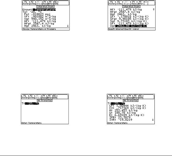
F2: Analysis/1: Steam Tables

Upper Display

Lower Display

All the calculated parameters are displayed on the screen with units attached as shown. The displayed results could be converted to other units as described in the first example described earlier.

Example 3.3:

Calculate the properties of dry air to be -20 ° C.

Select the Air Properties section. The input screen calls for defining the temperature. Enter a temperature of – 20 ° C. When entering -20 ° C, be sure to use the unary operator key – followed by 20 ° C. If you use\ key for a negative value this will result in an input error.

Press >to solve for the thermodynamic properties of air.

Input Screen

Result screen

All the calculated parameters are displayed on the screen with SI units attached as shown. The parameters computed can be viewed in other units as described in the examples shown here.

3.5 Validity Range for Temperature and Pressure

The computed results are valid only for the following finite ranges of temperature and pressure:

Saturated	Superheated
Temperature: 273.16 - 647.3 K	Saturated temperature
Pressure: 0.006113 - 22.08 MPa	Pressure: 0.006113 - 22.08 MPa

References:

1.Lester Haar, John S. Gallagher and George S. Kell, NBS/NRC Steam Tables, Thermodynamic and Transport Properties for Vapor and Liquid States of Water, Hemisphere Publishing Corporation, Washington, DC.

2.Steam Tables, 1967; Thermodynamic properties of Water and Steam, The Electric Research Association, Edward Arnold Limited, London England, 1967

3.Thomas F. Levine, Jr., and Peter E. Liley, Steam and Gas Tables with Computer Equations, Academic Press, New York, NY, 1984

ME Pro for TI -89, TI-92 Plus	25
Chapter 3 - Analysis – Steam Tables

F2: Analysis/ 2: Thermocouples

Chapter 4: Thermocouples

This chapter describes using the software in the Thermocouples menu. Thermocouple parameters are calculated for the class of thermocouples in common usage.

4.1 Introduction

This tool converts a specified temperature to an emf output, millivolts (mV), and from an emf output, millivolts (mV), to a specified temperature. The software supports Type T, E, J, K, S, R and B thermocouples. The underlying assumption is a reference temperature of 0° C. These computation algorithms result from the IPTS-68 standards adopted in 1968 and modified in 1985.

4.2 Using the Thermocouples Function

Select the Thermocouples function from the Analysis menu by highlighting Thermocouples and pressing ¸. This action brings out the main user interface screen. Press Bto view the choices available. Seven types of Thermocouples are available for computations. For example, to select a Pt-10%Rh-Pt thermocouple referred to as S Type thermocouple, move the high the highlight bar to Type S and press ¸or press z. At this point, the software presents the primary user interface awaiting data entry. At the same time, the material of the thermocouple and the valid range are displayed for reference.

Thermocouple computations involve computing emf available from a known temperature or computing a temperature from an emf. The latter case is by its very nature not as accurate as the first type of computation.

Screen 1 (for temperature)

Screen 2 (for emf)

Example 4.2:

Find the emf for an S type thermocouple at 400 ° F. From the value of emf computed, compute the temperature.

Solution 4.2:

Select Type S thermocouple for this problem. For temperature, enter 400, then press …. The computed emf is 1.4777mV. Now return to Known line and select emf for input. Enter 1.4777 mV for emf to get 403.989 ° F for temperature.

Notes: The thermocouple emf calculation can be expanded to cover the emf produced by the thermocouple if the reference temperature was different from 0 ° C. For example, if the reference temperature was 30 ° C instead of 0 ° C, you compute the resulting emf in two steps; first find the emf (emf 1) for the temperature desired, say 300 ° C, and the emf (emf 0) for the reference temperature. The resulting emf for the new reference temperature of 30 ° C is the difference between the two emf’s, i.e., "emf 1 - emf 0".

ME Pro for TI-89, TI-92Plus	26
Chapter 4 - Analysis - Thermocouples

F2: Analysis/ 2: Thermocouples

4.3 Basis for Temperature/Voltage Conversions

The temperature-to-voltage conversion is based on either a polynomial approximation or a combination of a polynomial coupled with a special sequence. This ensures precise calculations within some prescribed error range. These rages are displayed on each input screen.

References:

1.Robert L. Powell, William J. Hall, Clyde H. Hyink, Larry L. Sparks, George W. Burns, Margaret Scoger and Harmon H. Plumb, Thermocouple Reference Tables based on IPTS-68, NBS Monograph 125, Omega Press, 1975

ME Pro for TI-89, TI-92Plus	27
Chapter 4 - Analysis - Thermocouples

F2: Analysis/3: Capital Budgeting

Chapter 5: Capital Budgeting

This chapter covers the four basic measures of capital budgeting:

♦	Payback Period	♦	Internal Rate of Return
♦	Net Present Value	♦	Profitability Index

5.1 Using Capital Budgeting

This section performs analysis of capital e xpenditure for a project and compares projects against one another. Four measures of capital budgeting are included in this section: Payback period (Payback); Net Present Value (NPV); Internal Rate of Return (IRR); and Profitability Index (PI). This module provides the capability of entering, storing and editing capital expenditures for nine different projects. The following equations are used in calculations:

NPV =

∑n

CFt

− CFt

= 0

Eq. 1

k)

t

t = 1 (1 +

∑

n

CFt

−

CFt = 0 = 0

Eq. 2

+

IRR)

t

t = 1 (1

∑

n

CFt

t

PI =

t =

1

(1 +

k)

Eq. 3

CFt =

0

CFt: Cash Flow at time t.

Payback: The number of time periods it takes a firm to recover its original investment.

NPV: The present values of all future c ash flows, discounted at the selected rate, minus the cost of the investment.

IRR: The discount rate that equates the present value of expected cash flows to the initial cost of the project.

PI: The present value of the future cash flows, discounted at the selected rate, over the initial cash outlay.

ME Pro for TI-89, TI-92 Plus	28
Chapter 5 - Analysis - Capital Budgeting

		F2: Analysis/3: Capital Budgeting
	Field Descriptions - Input Screen
Project:	(Project)	Press —to select one of nine unique
		projects or edit the current name of the project
		by pressing efor Cash option.
k:	(Discount Rate per Period in %)	Enter a real number.
Payback:	(Payback Period)	Returns a real number.
npv:	(Net Present Value)	Returns a real number.
IRR:	(Internal Rate of Return)	Returns a real number (%).
PI:	(Profitability Index)	Returns a real number.
Multiple	(Graph multiple projects	Activation of this feature enables the overlay
Graphs	simultaneously)	of each successive graph (projects) on the
		same axis. Press —to activate.
Full	(Graph on full or split screen?)	Press —to activate.
Screen
Graph

Field Descriptions - Project Edit Screen

NAME:	(Project Name)
t0:	(Investment at t=0)
t1:	(Cash flow at t=1)
tn:	(Cash flow at t=n)

Enter the name of the project. Enter a real number.

Enter a positive or negative real number. Enter a positive or negative real number.

Example 5.1:

The following projects have been proposed by ACME Consolidated Inc. What are the Payback period, Net Present Value, Internal Rate of Return, and Profitability Index of each project? Which is the more viable project?

ME Pro for TI-89, TI-92 Plus	29
Chapter 5 - Analysis - Capital Budgeting

		F2: Analysis/3: Capital Budgeting
	Table 5-1 Cash Flow for two projects
Name of Project:	Plant 1	Plant 2
Investment Outlay:	$75,000 (at t=0)	$75,000 (at t=0)
Cost of Capital:	12%	12%
Year	Net Cash Flow ($)	Net Cash Flow ($)
0	-75,000	-75,000
1	40,000	10,000
2	30,000	20,000
3	20,000	30,000
4	10,000	40,000

Cash Flow Input: plant1

Cash Flow Input: plant2

Output Screen: plant1

Output Screen: plant2

1.With the highlight bar on the Project field, press — to select a project to edit. Select a project that has not been used. Note: this example uses projects 1 and 2. Press —to return to the Capital Budgeting screen.

2.Press eto select Cash option; enter the project edit screen; and, edit the cash flows.

3.Enter “plant1” in the Name field. Note: Cash flow data for this project will be stored in a variable of this name. Therefore the entered name must begin with a letter; be no more than 8 characters in length; and, contain no embedded spaces.

4.Press h5 times to add 5 time points and enter the cash flows at each time point from the table on the previous page. When finished, your screen should look like the project edit screen above. Be sure to enter 75,000 as a negative number for t0. Press .to save your changes and return to the Capital Budgeting screen.

5.Enter 12 for k.

6.Press cto calculate Payback, NPV, IRR, and PI.

7.Move the highlight bar to Multiple Graphs and press —to enable overlaying of successive graphs of each project.

8.Press dto graph the curvilinear relationship between the Net Present Value and the Discount Rate.

9.Press followed by /to enable the graph editing toolbar.

ME Pro for TI-89, TI-92 Plus	30
Chapter 5 - Analysis - Capital Budgeting