Texas instruments TI-30X PRO User Manual

TI-30X ProMathPrint™

ScientificCalculatorGuidebook

This guidebookapplies tosoftware version1.0. Toview the latest versionof the documentation, goto education.ti.com/eguide.

Important Information

Texas Instruments makes nowarranty, eitherexpress orimplied, including but not limitedtoanyimpliedwarranties of merchantabilityandfitness fora particular purpose, regarding anyprogrammes orbookmaterials andmakes suchmaterials available solelyonan"as-is" basis. Innoevent shall Texas Instruments be liable to anyone forspecial, collateral, incidental orconsequential damages inconnectionwith orarising from the purchase oruse of these materials, andthe sole andexclusive liabilityof Texas Instruments, regardless of the form of action, shall not exceedthe purchase price of this product. Moreover, Texas Instruments shall not be liable forany claim of anykindwhatsoeveragainst the use of these materials byanyotherparty.

MathPrint, APD, Automatic PowerDown, andEOS are trademarks of Texas Instruments Incorporated.

Copyright © 2018 Texas Instruments Incorporated

ii

Contents

GettingStarted	1
Switchingthe Calculator On and Off	1
Display Contrast	1
Home Screen	1
2nd Functions	2
Modes	2
Multi-Tap Keys	4
Menus	5
Examples	5
ScrollingExpressionsand History	6
Answer Toggle	6
Last Answer	7
Order ofOperations	7
Clearingand Correcting	9
Memory and Stored Variables	10

MathFunctions	13
Fractions	13
Percentages	15
Scientific Notation [EE]	16
Powers, Rootsand Inverses	17
Pi (symbol Pi)	17
Math	18
Number Functions	19
Angles	21
Rectangular to Polar	23
Trigonometry	24
Hyperbolics	26
Logarithm and Exponential Functions	26
Numerical Derivative	27
Numerical Integral	28
Statistics, Regressionsand Distributions	30
Probability	40

MathTools	43
Stored Operations	43
DataEditor and List Formulas	44
Function Table	48
Matrices	50
Vectors	53
Solvers	55

iii

Number Bases	60
Expression Evaluation	62
Constants	63
Conversions	64
Complex Numbers	67

Reference Information	70
Errorsand Messages	70
Battery Information	74
Troubleshooting	75

GeneralInformation	76
Online Help	76
Contact TI Support	76
Service and Warranty Information	76

iv

Getting Started

This sectioncontains informationabout basic calculatorfunctions.

Switching theCalculator On and Off

&turns onthe calculator. %'turns it off. The displayis cleared, but the history, settings, andmemoryare retained.

The APD™(Automatic PowerDown™) feature turns off the calculatorautomaticallyif nokeyis pressedforabout 3 minutes. Press &afterAPD™. The display, pending operations, settings, andmemoryare retained.

Display Contrast

The brightness andcontrast of the displaydependonroom lighting, batteryfreshness andviewing angle.

Toadjust the contrast:

1.Press andrelease the %key.

2.Press ](todarkenthe screen) or [(tolightenthe screen).

Note: This will adjust the contrast one level at a time. Repeat steps 1 and2 as needed.

HomeScreen

Onthe Home screen, youcanentermathematical expressions andfunctions, along withotherinstructions. The answers are displayedonthe Home screen.

The TI-30XProMathPrint™screencandisplaya maximum of fourlines witha maximum of 16 characters perline. Forentries andexpressions longerthanthe visible screenarea, youcanscroll left andright (!and ") toview the entire entryor expression.

InMathPrint™mode, youcanenteruptofourlevels of consecutive nestedfunctions

andexpressions, whichinclude fractions, square roots, exponents with^, Ü, ex, and 10x.

Whenyoucalculate anentryonthe Home screen, depending uponspace, the answeris displayedeitherdirectlytothe right of the entryoronthe right side of the next line.

Special indicators andcursors maybe displayedonthe screentoprovide additional informationconcerning functions orresults.

Indicator	Definition
2ND	2ndfunction.
FIX	Fixed-decimal setting. (See Mode section.)
SCI, ENG	Scientific orengineering notation. (See Mode
	section.)

GettingStarted 1

Indicator	Definition
DEG, RAD,	Angle mode (degrees, radians, orgradians). (See
GRAD	Mode section.)
L1, L2, L3	Displays above the lists indata editor.
H, B, O	Indicates HEX, BIN, orOCT number-base mode. No
	indicatordisplayedfordefault DECmode.
	The calculatoris performing anoperation. Use &
	tobreakthe calculation.
5 6	Anentryis storedinmemorybefore and/orafter
	the visible screenarea. Press #and $toscroll.
´	Indicates that the multi-tapkeyis active.
	Normal cursor. Shows where the next item you
	type will appear. Replaces anycurrent character.
	Entry-limit cursor. Noadditional characters canbe
	entered.
	Insert cursor. A characteris insertedinfront of the
	cursorlocation.
	PlaceholderboxforemptyMathPrint™template.
	Use the arrow keys tomove intothe box.
	MathPrint™cursor. Continue entering inthe
	current MathPrint™template, orpress "toexit
	the template.

2nd Functions

%

Most keys canperform more thanone function. The primaryfunctionis indicatedon the keyandthe secondaryfunctionis displayedabove it. Press %toenable the secondaryfunctionof a givenkey. Notice that 2ND appears as anindicatoronthe screen. Tocancel before pressing the next key, press %again. Forexample, %b 25 <calculates the square root of 25 andreturns the result, 5.

Modes

q

Use qtochoose modes. Press $#!"tochoose a mode, and <toselect it. Press -or %storeturntothe Home screenandperform yourworkusing the chosenmode settings.

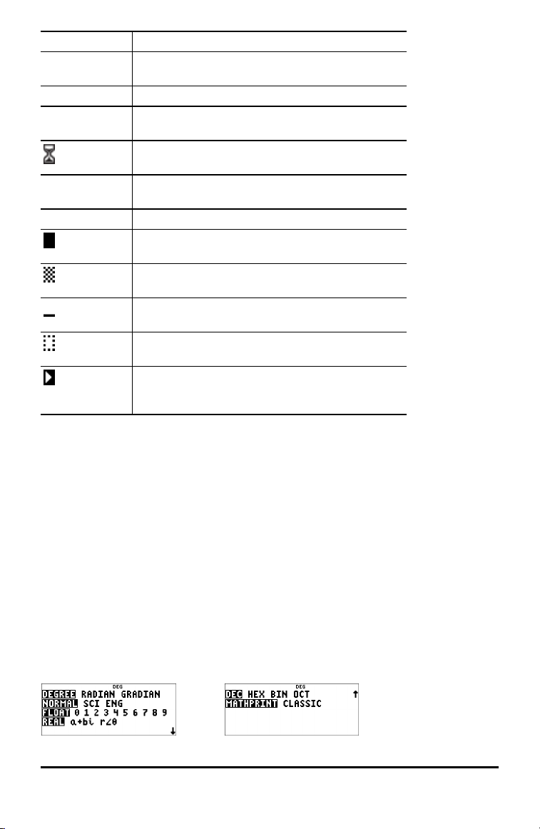
Default settings are highlightedinthese sample screens.

2 GettingStarted

DEGREE	RADIAN GRADIAN - Sets the angle mode todegrees, radians, orgradians.
NORMAL	SCI ENG - Sets the numeric notationmode. Numeric notationmodes

affect onlythe displayof results, andnot the accuracyof the values storedinthe unit, whichremainmaximal.

NORMAL displays results withdigits tothe left andright of the decimal, as in 123456.78.

SCI expresses numbers withone digit tothe left of the decimal andthe appropriate powerof 10, as in1.2345678E5, whichis the same as the value (1.2345678×105) including the brackets forcorrect orderof operation.

ENG displays results as a numberfrom 1 to999 times 10 toanintegerpower. The integerpoweris always a multiple of 3.

Note: Eis a shortcut keytoentera numberinscientific notationformat. The result displays inthe numeric notationformat selectedinthe mode menu.

FLOAT 0 1 2 3 4 5 6 7 8 9 - Sets the decimal notationmode.

Float (floating) decimal mode displays upto10 digits, plus the signanddecimal.

0 1 2 3 4 5 6 7 8 9 (fixeddecimal point) specifies the numberof digits (0 to9) to displaytothe right of the decimal.

REAL	a+bi	r±q - Sets the format of complexnumberresults.
REAL real results
a+bi rectangularresults
r±q polarresults
DEC	HEX	BIN OCT - Sets the numberbase usedforcalculations.

DEC decimal

HEX hexadecimal (Toenterhexdigits A throughF, use %§, %¨, andsoon.)

BIN binary

OCT octal

MATHPRINT CLASSIC

MATHPRINT mode displays most inputs andoutputs intextbookformat.

CLASSIC mode displays inputs andoutputs ina single line.

Examples of MathPrint™ andClassic Modes

MathPrint™ Mode	Classic Mode
Sci	Sci

GettingStarted 3

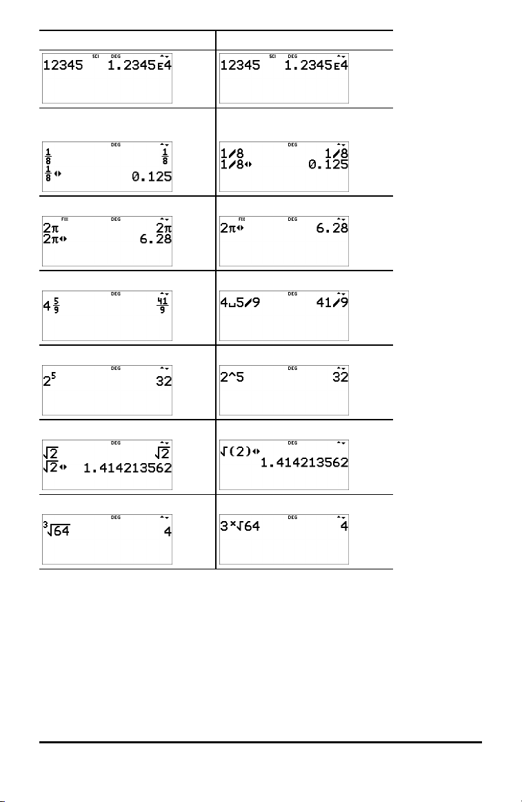
MathPrint™ Mode

Classic Mode

Float mode andanswertoggle	Float mode andanswertoggle
key	key.

Fix2 andanswertoggle key

Fix2

Un/d

Un/dentry

Exponent example

Exponent example

Square root example

Square root example

Cube root example

Cube root example

Multi-Tap Keys

A multi-tapkeyis one that cycles throughmultiple functions whenyoupress it. Press "tostopmulti-tap.

Forexample, the Xkeycontains the trigonometryfunctions sin and sin/ as well as the hyperbolic functions sinh and sinh/. Press the keyrepeatedlytodisplaythe function that youwant toenter.

4 GettingStarted

Multi-tapkeys include z, X, Y, Z, C, D, H, and g. Applicable sections of this guidebookdescribe how touse the keys.

Menus

Menus give youaccess toa large numberof calculatorfunctions. Some menukeys, suchas %h, displaya single menu. Others, suchas d, displaymultiple menus.

Press "and $toscroll andselect a menuitem, orpress the corresponding number next tothe item. Toreturntothe previous screenwithout selecting the item, press -. Toexit a menuandreturntothe Home screen, press %s.

%h(keywitha single menu):

RECALL VAR

1:x= 0 2:y= 0 3:z = 0 4:t = 0 5:a = 0 6:b= 0 7:c = 0 8:d= 0

d(keywithmultiple menus):

MATHS	NUM	DMS	R³´P
1:4n/d³´Un/d	1:abs(	1:¡	1:P 4 Rx(
2:lcm(	2:round(	2:¢	2:P 4 Ry(
3:gcd(	3:iPart(	3:£	3:R 4	Pr(
4:4Pfactor	4:fPart(	4:r	4:R 4	Pq(
5:sum(	5:int(	5:g
6:prod(	6:min(	6:4DMS
7:nDeriv(	7:max(
8:fnInt(	8:mod(

Examples

Some sections are followedbyinstructions forkeystroke examples that demonstrate the TI-30XProMathPrint™functions.

Notes:

•Examples assume all default settings, as showninthe Modes sectionunless noted inthe example.

•Use -toclearthe home screenas needed.

GettingStarted 5

•Some screenelements maydifferfrom those showninthis document.

•Since wizards retaintheirmemory, some keystrokes maybe different.

Scrolling Expressions and History

!"#$

Press !or "tomove the cursorwithinanexpressionthat youare entering orediting. Press %!or %"tomove the cursordirectlytothe beginning orendof the expression.

From anexpressionoredit, #moves the cursortothe history. Press <from an input oroutput inhistorytopaste that expressionbacktothe cursorpositiononthe edit line.

Press %#from the denominatorof a fractioninthe expressions edit tomove the cursortothe history. Press <from aninput oroutput inhistorytopaste that expressionbacktothe cursorpositiononthe edit line.

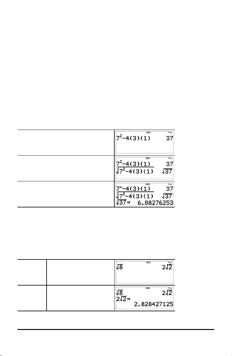
Example

7 FU4

(3 )(1 )<

%b##<

<

r

Answer Toggle

r

Press the rkeytotoggle the displayresult (whenpossible) betweenfractionand decimal answers, exact square root anddecimal, andexact pi anddecimal.

Example

Answer %b8 < toggle

r

6 GettingStarted

Note: ris alsoavailable totoggle numberformats forvalues incells inthe Function Table andinthe Data Editor. Editors suchas inmatrix, vectorandsystem solverwill displaytoggledcell values.

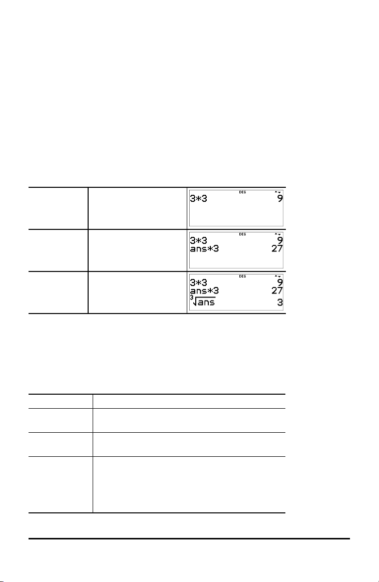
Last Answer

%i

The last entryperformedonthe home screenis storedtothe variable ans. This variable is retainedinmemory, evenafterthe calculatoris turnedoff. Torecall the value of ans:

•Press %i(ans displays onthe screen), or

•Press anyoperations key(T, U, andsoforth) inmost edit lines as the first part of anentry. ans andthe operatorare bothdisplayed.

Examples

ans 3 V3 <

V3 <

3 %c%i

<

Note: The variable ans is storedandpastes infull precisionwhichis 13 digits.

Order of Operations

The TI-30XProMathPrint™calculatoruses EquationOperating System (EOS™) to evaluate expressions. Withina prioritylevel, EOS™evaluates functions from left to right andinthe following order.

1st	Expressions inside brackets.
2nd	Functions that needa ) andprecede the argument,
	suchas sin, log, andall R³´P menuitems.
3rd	Functions that are enteredafterthe argument,
	suchas x2 andangle unit modifiers.
4th	Exponentiation(^) androots (x ‡).
	Note: InClassic mode, exponentiationusing the
	Gkeyis evaluatedfrom left toright. The
	expression2^3^2 is evaluatedas (2^3)^2, witha
	result of 64.

GettingStarted 7

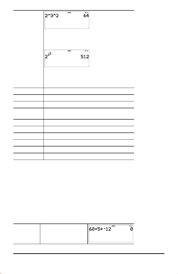
InMathPrint™mode, exponentiationusing the G keyis evaluatedfrom right toleft. The expression 2^3^2 is evaluatedas 2^(3^2), witha result of 512.

	The calculatorevaluates expressions enteredwith
	F and afrom left toright inbothClassic and
	MathPrint™modes. Pressing 3 FF is
	calculatedas (32)2 = 81.
5th	Negation(M).
6th	Fractions.
7th	Permutations (nPr) andcombinations (nCr).
8th	Multiplication, impliedmultiplication, division, and
	angle indicator ±.
9th	Additionandsubtraction.
10th	Logic operators and, nand.
11th	Logic operators or, xor, xnor.
12th	Conversions suchas 4n/d³´Un/d, F³´D, 4DMS.
13th	L
14th	<evaluates the input expression.

Note: Endof expressionoperators andBase nconversions suchas 4Bin, angle conversion 4DMS, 4Pfactor, andcomplexnumberconversions 4Polar and 4Rectangle, are onlyvalidinthe Home Screen. Theyare ignoredinwizards, functiontable displayand data editorfeatures where the expressionresult, if valid, will displaywithout a conversion. Editors suchas inmatrix, vectorandsystem solverwill alsoignore these endof expressionoperators inthe edit line.

Note: Use brackets toclearlyindicate the operationorderyouexpect foryour expressionentry. If necessary, the brackets canbe usedtooverride the orderof operations followedbythe algorithms inthe calculator. If the result is not as expected, checkhow the expressionwas enteredandaddbrackets as needed.

Examples

+ Q P M 60 T5 VM12 <

8 GettingStarted

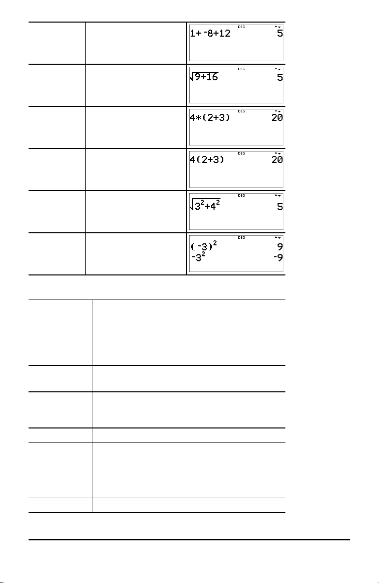
(M)	1	TM8 T12 <
‡ and+	%b9		T16 <
( )	4	V(2	T3 )<
( ) and+	4	(2 T3 )<
^ and ‡	%b3		G2 "T4
	G2 <
( ) and M	(M3 )F<
	M3 F<

Clearing and Correcting

%s	Returns the cursortothe home screen.
	Quicklydismisses these applications:Expression
	Evaluation, Set Operation, FunctionTable, Data
	Editor, Statistics, Distributions, Vector, Matrix,
	Numeric Solver, Polynomial Solver, andSystem
	Solver.

-Clears anerrormessage. Clears characters onentryline.

JDeletes the characterat the cursor.

Whenthe cursoris at the endof anexpression, it will backspace anddelete.

%f Inserts a characterat the cursor.

%{1 Clears variables x, y, z, t, a, b, c, and d totheir default value of 0.

AnycomputedStat Vars will nolongerbe available inthe Stat Vars menu. Recompute statistic features as needed.

% 2	Resets the calculator.

GettingStarted 9

Returns the calculatortodefault settings;clears memoryvariables, pending operations, all entries inhistoryandstatistical data;clears anystored operationand ans.

Memory and Stored Variables

z L %h %{

The TI-30XProMathPrint™calculatorhas 8 memoryvariables—x, y, z, t, a, b, c, and d. Youcanstore the following toa memoryvariable:

•real orcomplexnumbers

•expressionresults

•calculations from various applications suchas Distributions

•data editorcell values (storedfrom the edit line)

Features of the calculatorthat use variables will use the values that youstore.

Llets youstore values tovariables. Press Ltostore a variable, andpress z toselect the variable tostore. Press <tostore the value inthe selectedvariable. If this variable alreadyhas a value, that value is replacedbythe new one.

z is a multi-tapkeythat cycles throughthe variable names x, y, z, t, a, b, c, and d. Youcanalsouse z torecall the storedvalues forthese variables. The name of the variable is enteredinthe current entry, but the value assignedtothe variable is usedto evaluate the expression. Toentertwoormore variables insuccession, press "after each.

%hrecalls the values of variables. Press %htodisplaya menuof variables andtheirstoredvalues. Select the variable youwant torecall andpress <. The value assignedtothe variable is insertedintothe current entryandusedto evaluate the expression.

%{clears variable values. Press %{andselect 1:Yes toclearall variable values. AnycomputedStat Vars will nolongerbe available inthe Stat Vars menu. Recompute statistic features as needed.

Examples

Start with %s- clear

screen

ClearVar %{

1 (Selects Yes)

10 GettingStarted

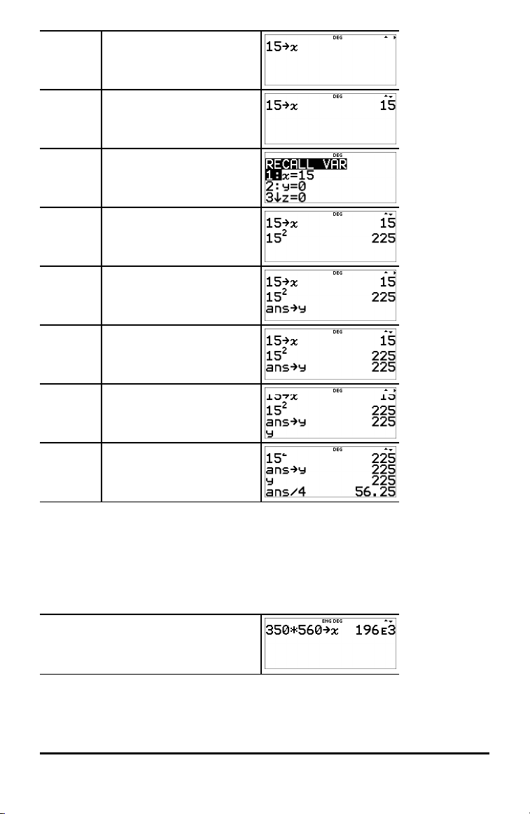
Store 15 Lz

<

Recall %h

<F<

Lzz

<

zz

<W4 <

³ Problem

Ina gravel quarry, twonew excavations have beenopened. The first one measures 350 metres by560 metres, the secondone measures 340 metres by610 metres. What volume of gravel does the companyneedtoextract from eachexcavationtoreacha depthof 150 metres? Toreach210 metres? Displaythe results inengineering notation.

q$""<-

350 V560 Lz<

GettingStarted 11

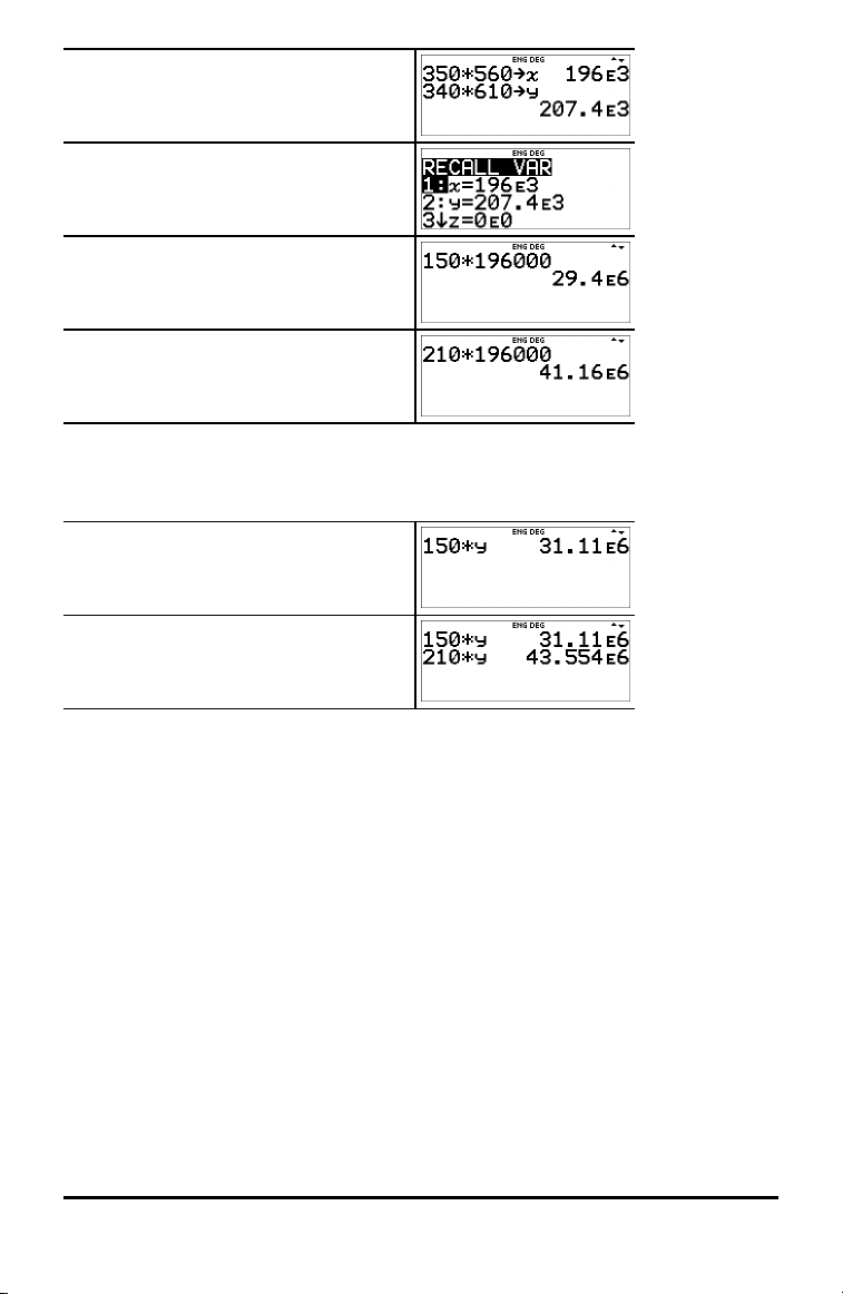
340 V610 Lzz<

-

150 V%h

<<

-

210 V%h<<

Forthe first excavation, the companyneeds toextract 29.4 millioncubic metres to reacha depthof 150 metres, andextract 41.16 millioncubic metres toreacha depth of 210 metres.

-

150 Vzz<

210 Vzz<

Forthe secondexcavation, the companyneeds toextract 31.11 millioncubic metres to reacha depthof 150 metres, andextract 43.554 millioncubic metres toreacha depth of 210 metres.

12 GettingStarted

Math Functions

This sectioncontains informationabout using the calculatormaths functions suchas trigonometry, statistics andprobability.

Fractions

P%@ d1 %j

Fractions with Pcaninclude real andcomplexnumbers, operationkeys (T, V, etc.), andmost functionkeys (F, %_, etc.).

InClassic mode orclassic entries inMathPrint™mode, the fractionbar Pdisplays inline as a thickbar, forexample . Use brackets toclearlyindicate the arithmetic you expect. While the Orderof Operations rules will apply, youare incontrol of the wayan expressionevaluates byplacing the correct brackets inyourinputs.

FractionResults

•Fractionresults are automaticallysimplifiedandoutput is inimproperfraction format.

•Whenmixednumberoutput is desired, use the 4n/d³´Un/dmixednumber conversionat the endof the input expression. This feature is locatedin d1:

4n/d³´Un/d.

•Fractionresults are obtainedwhenthe calculatedvalue candisplaywithinthe limits of the fractionformat supportedbythe calculatorandnodecimal value was enteredinthe input expression.

•If decimal numbers are usedorcalculatedina fractionnumeratorordenominator, the result will displayas a decimal. Entering a decimal forces the result todisplay indecimal format.

•Use %j (above r) onresults toattempt fractiontodecimal conversions withinthe fractiondisplaylimits offeredbythis numeric calculator.

MixedNumbers andConversions

•%@enters a mixednumber. Press the arrow keys tocycle throughthe unit, numerator, anddenominator.

•d1 converts betweensimple fractions andmixed-numberform (4n/d³´Un/d).

•%j converts results betweenfractions anddecimals.

MathPrint™ Entry

•Toenternumbers orexpressions inthe numeratoranddenominatorinMathPrint™ mode, press P.

•Press $or #tomove the cursorbetweenthe numeratoranddenominator.

•Pressing Pbefore orafternumbers orfunctions maypre-populate the numerator withparts of yourexpression. Watchthe screenas youpress keys toensure you enterthe expressionexactlyas needed.

MathFunctions 13

Onthe Home Screen

•Topaste a previous entryfrom historyinthe numeratorormixednumberunit, place the cursorinthe numeratororunit, press #toscroll tothe desiredentry, andthenpress <topaste the entrytothe numeratororunit.

•Topaste a previous entryfrom historyinthe denominator, place the cursorinthe denominator, press %#tojumpintohistory. Press #toscroll tothe desired entry, andthenpress <topaste the entrytothe denominator.

Evaluationof YourExpression

•When <is pressedtoevaluate yourinput expression, brackets maybe displayed toclearlyindicate how it was interpretedandcalculatedbythe calculator. If it is not what youexpected, copythe input expressionandedit as needed.

Classic Mode orClassic Entry

•If the cursoris ina classic entrylocation, enterthe numeratorexpressionenclosed bybrackets, thenpress Ptodisplaythe thickfractionbar, andthenenterthe denominatorexpressionalsoenclosedwithbrackets forthe result tobe calculated as youexpect foryourproblem.

Examples inMathPrint™ Mode

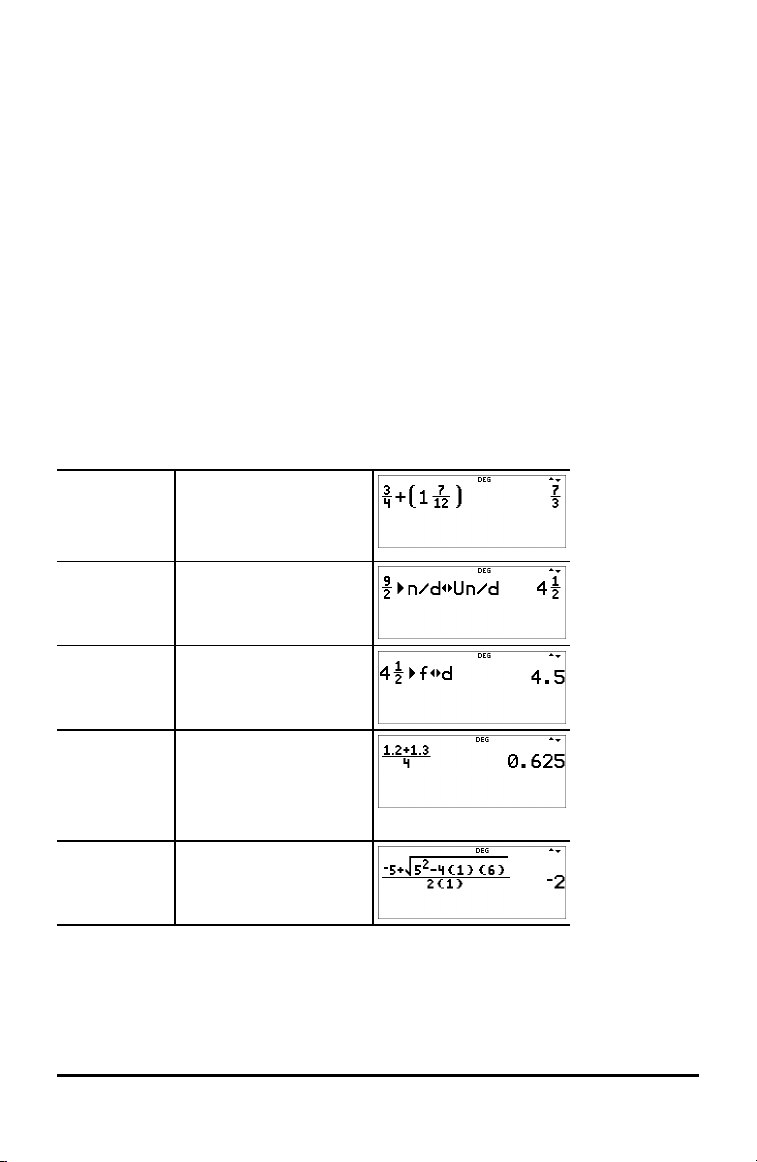
n/d, Un/d	P3 $4 "T1 %
	@7 $12 <
	Note: Brackets are added
	automatically.
4n/d³´Un/d	9 P2 "d1 <
f³´d	4 %@1	$2 "%
	j <
Example	P1.2 T1.3	$4 <
	Note: Result is decimal
	since decimal numbers
	were usedinthe
	fraction.
Example	PM5 T%b5
	FU4 (1 )(6 )
	$2 (1 )<

14 MathFunctions

Examples inClassic Mode

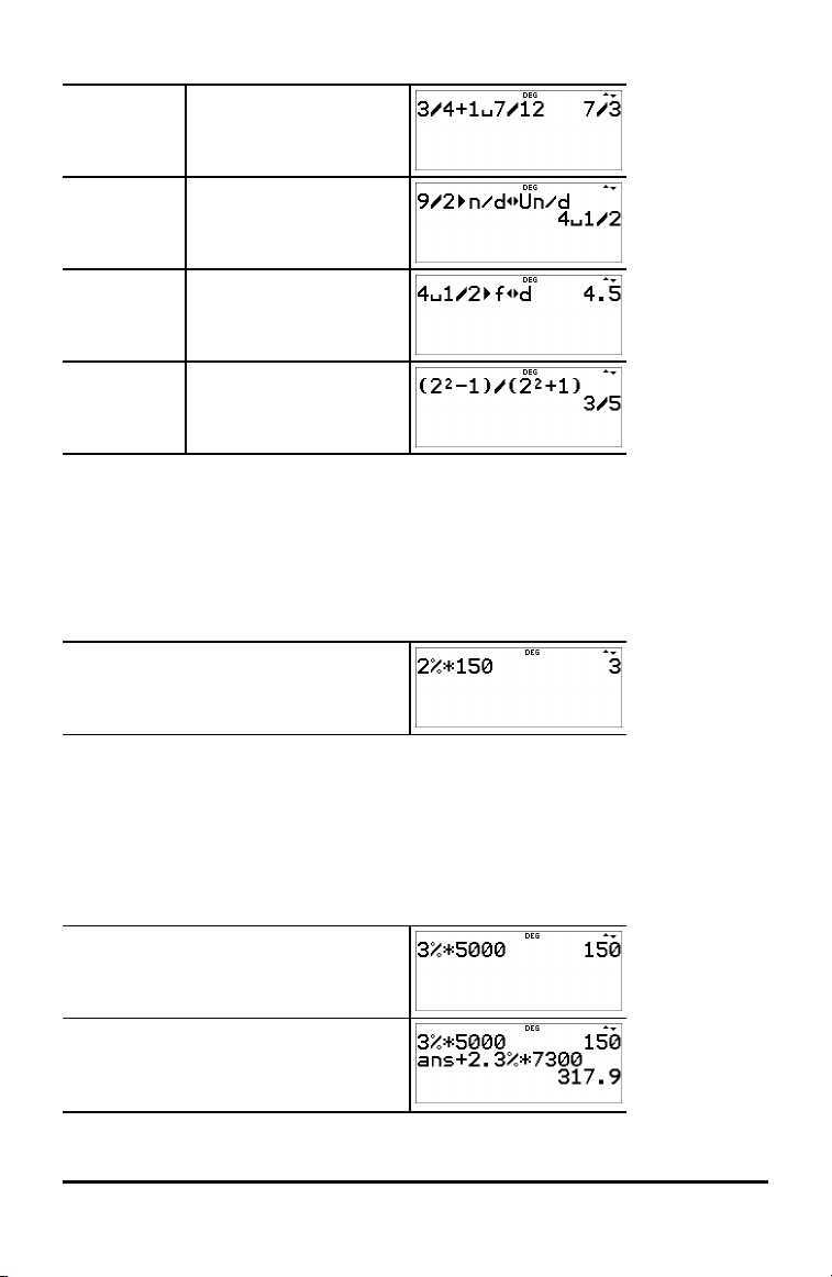
n/d, Un/d 3 P4 T1 %@7 P

12 <

4n/d³´Un/d 9 P2 d1 <

f³´d 4 %@1 P2 % j <

Brackets (2 FU1 )P(2

FT1 )<

Percentages

%_

Toperform a calculationinvolving a percentage, press %_afterentering the value of the percentage.

Example

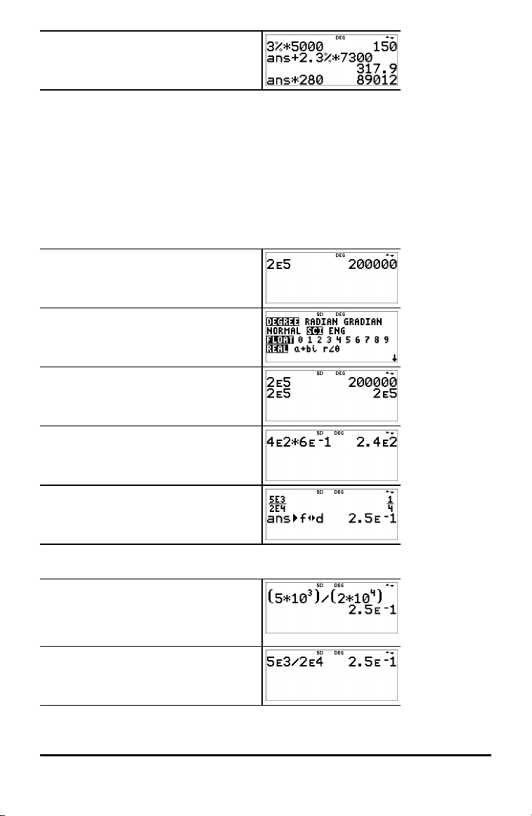
2 %_V150 <

³ Problem

A mining companyextracts 5000 tonnes of ore witha concentrationof metal of 3% and7300 tonnes witha concentrationof 2.3%. Onthe basis of these twoextraction figures, what is the total quantityof metal obtained?

If one tonne of metal is worth280 units of currency, what is the total value of the metal extracted?

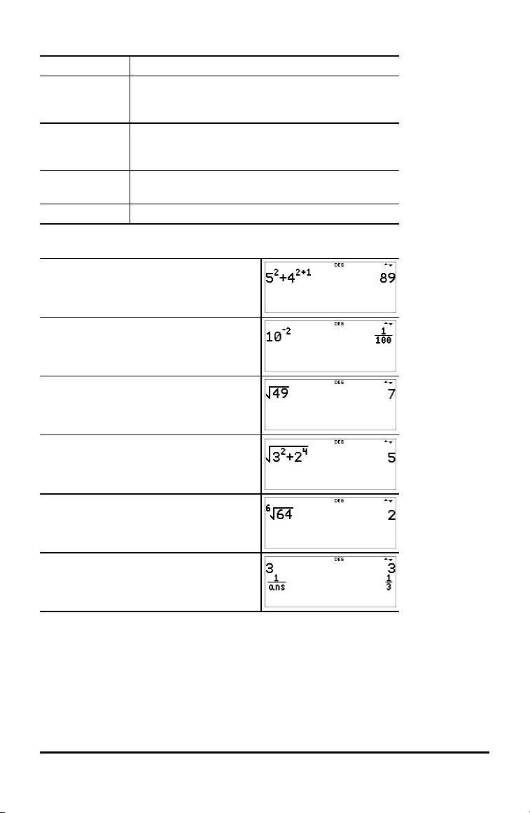
3 %_V5000 <

T2.3 %_V7300 <

MathFunctions 15

V280 <

The twoextractions represent a total of 317.9 tonnes of metal fora total value of 89012 units of currency.

Scientific Notation [EE]

E

Eis a shortcut keytoentera numberinscientific notationformat. A numbersuchas (1.2 x10-4) is enteredinthe calculatoras the number1.2E-4.

Example

2 E5 <

Note: Enters (2 x105) using the calculator E notation.

q$"<

Note: The SCI mode setting displays results inscientific notation.

-<

-

4 E2 V6 EM1 <

P5 E3 $2 E4 < %i%j

Example

TextbookProblem

-

(5 V10 G3 ")W(2 V10 G 4 ")<

Using E

-

5 E3 W2 E4 <

16 MathFunctions

Powers, Roots and Inverses

FCalculates the square of a value.

GRaises a value tothe powerindicated. Use "to move the cursorout of the powerinMathPrint™ mode.

%b	Calculates the square root of a non-negative value.
	Incomplexnumbermodes, a+bi andr±q,
	calculates the square root of a negative real value.
%c	Calculates the xthroot of anynon-negative value
	andanyoddintegerroot of a negative value.

aInverts the enteredvalue as 1/x.

Examples

5 FT4 G2 T1 "

<

10 GM2 <

%b49 <

%b3 FT2 G4 <

6 %c64 <

3 <%a<

Pi (symbol Pi)

g(multi-tapkey)

p ≈ 3.14159265359 forcalculations.

p ≈ 3.141592654 fordisplayinFloat mode.

MathFunctions 17

Example

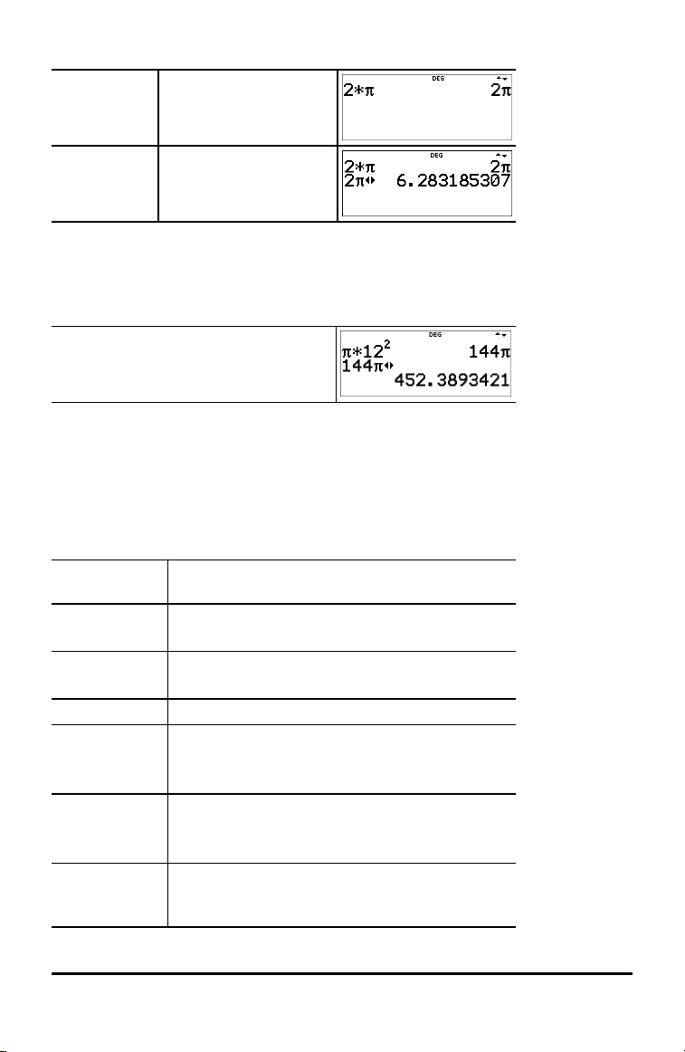
p2 Vg<

r

³Problem

What is the area of a circle if the radius is 12 cm?

Reminder:A = p×r2

gV12 F< r

The area of the circle is 144 p square cm. The area of the circle is approximately452.4 square cm whenroundedtoone decimal place.

Math

dMATH

ddisplays the MATH menu:

1:4n/d³´Un/d	Converts betweensimple fractions andmixed-
	numberform.
2:lcm(	Least commonmultiple
	Syntax: lcm(valueA,valueB)
3:gcd(	Greatest commondivisor
	Syntax: gcd(valueA,valueB)
4:4Pfactor	Prime factors
5:sum(	Summation
	Syntax: sum(expression,variable,lower,upper)
	(Classic mode syntax)
6:prod(	Product
	Syntax: prod(expression,variable,lower,upper)
	(Classic mode syntax)
7:nDeriv(	Numerical derivative at a point withoptional
	tolerance argument, H, whencommandis usedin
	Classic mode, classic entry, andinMathPrint™

18 MathFunctions

	mode.
	Syntax: nDeriv(expression,variable,point
	[,tolerance])
	(Classic mode syntax)
8:fnInt(	Numerical integral overaninterval withoptional
	tolerance argument, H, whencommandis usedin
	Classic mode, classic entry, andinMathPrint™
	mode.
	Syntax: fnInt(expression,variable,lower,upper
	[,tolerance])
	(Classic mode syntax)
Examples
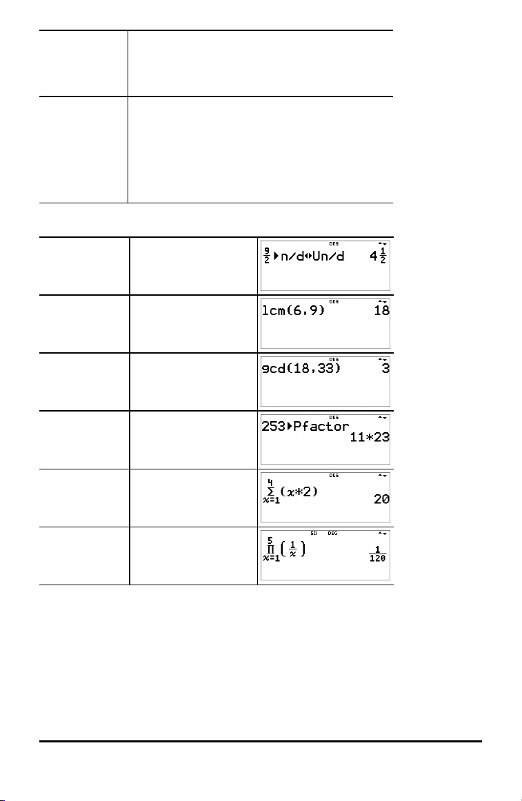
4n/d³´Un/d	9 P2 "d1 <
lcm(	d2
	6 %`9 )<
gcd(	d3
	18 %`33 )<
4Pfactor	253 d4 <
sum(	d5
	1 "4 "zV2
	<
prod(	d6
	1 "5 "1 Pz
	""<

Note: See Numerical Derivative, nDeriv(, andNumerical Integral, fnInt( inMaths Functions forexamples andmore information.

Number Functions

dNUM

d"displays the NUM menu:

MathFunctions 19

1:abs(		Absolute value
		Syntax: abs(value)
2:round(		Roundedvalue
		Syntax: round(value,#decimals)
3:iPart(		Integerpart of a number
		Syntax: iPart(value)
4:fPart(		Fractional part of a number
		Syntax: fPart(value)
5:int(		Greatest integerthat is { the number
		Syntax: int(value)
6:min(		Minimum of twonumbers
		Syntax: min(valueA,valueB)
7:max(		Maximum of twonumbers
		Syntax: max(valueA,valueB)
8:mod(		Modulo(remainderof first number P second
		number)
		Syntax: mod(dividend,divisor)
Examples
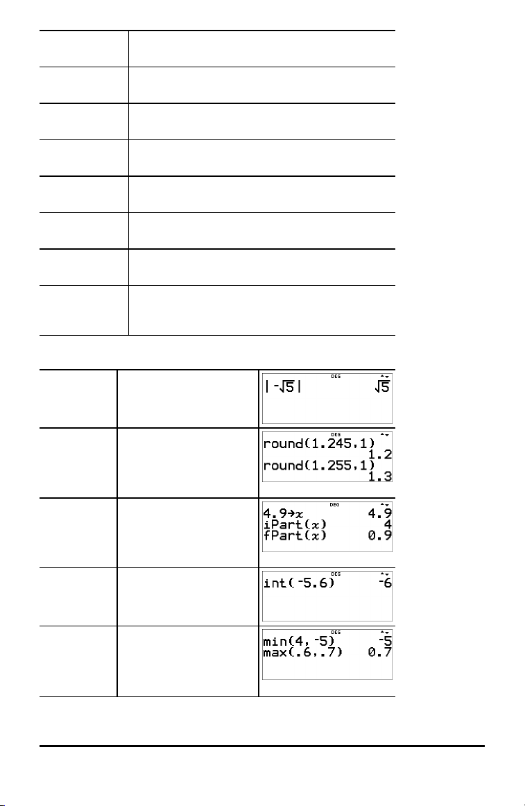
abs(	d"1
	M%b5 <
round(	d"2
	1.245 %`1 )<
	##<
	!!!!!5 <
iPart(	4.9 Lz<
fPart(	d"3 z)<
	d"4 z)
	<
int(	d"5
	M5.6 )<
min(	d"6
max(	4 %`M5 )<
	d"7
	.6 %`.7 )<

20 MathFunctions