HP 54600 schematic

4 (3)

Programmer’s Guide

Publication number 54600-97032

April 2001

This guide contains programming information for the following Agilent oscilloscope models:

54600

54601

54602

54603

54610

54615

54616

For Safety information, Warranties, and Regulatory information, see the pages behind the Index.

Agilent 54600-Series

Oscilloscopes

Programming the Oscilloscope

When you attach an interface module to the rear of the Agilent 54600Series Oscilloscopes, the oscilloscope becomes programmable. That is, you can hook a controller (such as a PC or workstation) to the oscilloscope, and write programs on that controller to automate oscilloscope setup and data capture. Both GPIB (also known as IEEE-488) and RS-232-C interfaces are available.

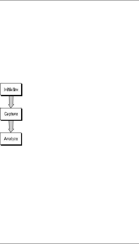
The following figure shows the basic structure of every program you will write for the oscilloscope.

Initialize

To ensure consistent, repeatable performance, you need to start the program, controller, and oscilloscope in a known state. Without correct initialization, your program may run correctly in one instance and not in another. This might be due to changes made in configuration by previous program runs or from the front panel of the oscilloscope.

·Program initialization defines and initializes variables, allocates memory, or tests system configuration.

·Controller initialization ensures that the interface to the oscilloscope (either GPIB or RS-232) is properly setup and ready for data transfer.

·Oscilloscope initialization sets the channel, trigger, timebase, and acquisition subsystems for the desired measurement.

Capture

Once you initialize the oscilloscope, you can begin capturing data for measurement. Remember that while the oscilloscope is responding to commands from the controller, it is not performing acquisitions. Also, when you change the oscilloscope configuration, any data already captured is most likely invalid.

To collect data, you use the DIGITIZE command. This command clears the waveform buffers and starts the acquisition process. Acquisition continues until the criteria, such as number of averages, completion criteria, and number of points is satisfied. Once the criteria is satisfied, the acquisition process is stopped. The acquired data is displayed by the oscilloscope, and the captured data can be measured, stored in memory in the oscilloscope, or transferred to the controller for further analysis. Any additional commands sent while DIGITIZE is working are buffered until DIGITIZE is complete.

You could also start the oscilloscope running, then use a wait loop in your program to ensure that the oscilloscope has completed at least one acquisition before you make a measurement. This is not recommended, because the needed length of the wait loop may vary, causing your program to fail. DIGITIZE, on the other hand, ensures that data capture is complete. Also, DIGITIZE, when complete, stops the acquisition process, so that all measurements are on displayed data, not a constantly changing data set.

Analyze

After the oscilloscope has completed an acquisition, you can find out more about the data, either by using the oscilloscope measurements or by transferring the data to the controller for manipulation by your program. Built-in measurements include IEEE standard parametric measurements (such as Vpp, frequency, pulse width) or the positioning and reading of voltage and time markers.

Using the WAVEFORM commands, you can transfer the data to your controller for special analysis, if desired.

iii

In This Book

The Agilent 54600-Series Oscilloscopes Programmer’s Guide is your introduction to programming the Agilent 54600-Series Oscilloscopes using an instrument controller. This book, with the online Agilent 54600-Series Oscilloscopes Programmer’s Reference, provides a comprehensive description of the oscilloscope’s programmatic interface. The Programmer’s Reference is supplied as a Microsoft Windows Help file on a 3.5" diskette.

To program the Agilent 54600-Series Oscilloscope, you need an interface module, such as the Agilent 54650A or 54651A. You also need an instrument controller that supports either the IEEE-488 or RS-232-C interface standards, and a programming language capable of communicating with these interfaces. You can also use the Agilent 54655A/56A Test Automation Module and the Agilent 54658A/59B Measurement/Storage Module.

Chapter 1 gives a general overview of oscilloscope programming.

Chapter 2 shows a simple program, explains its operation, and discusses considerations for data types.

Chapter 3 discusses the general considerations for programming the instrument over an GPIB interface.

Chapter 4 discusses the general considerations for programming the instrument over an RS-232-C interface.

Chapter 5 describes conventions used in representing syntax of commands throughout this book and in the online Agilent 54600-Series Oscilloscopes Programmer’s Reference, and gives an overview of the command set.

Chapter 6 discusses the oscilloscope status registers and how to use them in your programs.

Chapter 7 tells how to install the Agilent 54600-Series Oscilloscopes Programmer’s Reference online help file in Microsoft Windows, and explains help file navigation.

Chapter 8 lists all the commands and queries available for programming the oscilloscope.

For information on oscilloscope operation, see the Agilent 54600-Series Oscilloscopes User and Service Guide. For information on interface configuration, see the documentation for the oscilloscope and the interface card used in your controller (for example, the 82341C interface for IBM PC-compatible computers).

1	Introduction to Programming


2	Programming Getting Started


3	Programming over GPIB


4	Programming over RS-232-C


5	Programming and
5	Documentation Conventions
	Documentation Conventions


6	Status Reporting


7	Installing and Using the
7	Programmer’s Reference
	Programmer’s Reference


8	Programmer’s Quick Reference


	Index

1Introduction to Programming

Talking to the Instrument 1–3 Program Message Syntax 1–4

Combining Commands from the Same Subsystem 1–7 Duplicate Mnemonics 1–7

Query Command 1–8 Program Header Options 1–9

Program Data Syntax Rules 1–10 Program Message Terminator 1–12 Selecting Multiple Subsystems 1–12

2Programming Getting Started

Initialization 2–3 Autoscale 2–4

Setting Up the Instrument 2–4 Example Program 2–5

Using the DIGitize Command 2–6

Receiving Information from the Instrument 2–8 String Variables 2–9

Numeric Variables 2–10

Definite-Length Block Response Data 2–11 Multiple Queries 2–12

Instrument Status 2–12

3Programming over GPIB

Interface Capabilities 3–3 Command and data concepts 3–3 Addressing 3–4

Communicating over the bus 3–5 Lockout 3–6

Bus Commands 3–6

4Programming over RS-232-C

Interface Operation 4–3 Cables 4–3

Contents–1

Contents

Minimum three-wire interface with software protocol 4–4 Extended interface with hardware handshake 4–5 Configuring the Interface 4–7

Interface Capabilities 4–8

Communicating over the RS-232-C bus 4–9 Lockout Command 4–10

5Programming and Documentation Conventions

Command Set Organization 5–3 The Command Tree 5–6 Truncation Rules 5–10

Infinity Representation 5–11

Sequential and Overlapped Commands 5–11

Response Generation 5–11

Notation Conventions and Definitions 5–12

Program Examples 5–13

6Status Reporting

Serial Poll 6–6

7 Installing and Using the Programmer’s Reference

To install the help file under Microsoft Windows 7–3

To get updated help and program files via the Internet 7–4 To start the help file 7–5

To navigate through the help file 7–6

8Programmer’s Quick Reference

Conventions 8–3 Suffix Multipliers 8–3

Commands and Queries 8–4

Index

Contents–2

Introduction to Programming

Chapters 1 and 2 introduce the basics for remote programming of an oscilloscope. The programming instructions in this manual conform to the IEEE 488.2 Standard Digital Interface for Programmable Instrumentation. The programming instructions provide the means of remote control.

To program the Agilent 54600-series oscilloscope you must add either an GPIB (for example, Agilent 54650A) or RS-232-C (for example, Agilent 54651A) interface to the rear panel.

You can perform the following basic operations with a controller and an oscilloscope:

·Set up the instrument.

·Make measurements.

·Get data (waveform, measurements, configuration) from the oscilloscope.

·Send information (pixel image, configurations) to the oscilloscope. Other tasks are accomplished by combining these basic functions.

Languages for Program Examples

The programming examples for individual commands in this manual are written in Agilent BASIC, C, or SICL C.

1–2

Introduction to Programming

Talking to the Instrument

Computers acting as controllers communicate with the instrument by sending and receiving messages over a remote interface. Instructions for programming normally appear as ASCII character strings embedded inside the output statements of a “host” language available on your controller. The input statements of the host language are used to read in responses from the oscilloscope.

For example, Agilent BASIC uses the OUTPUT statement for sending commands and queries. After a query is sent, the response is usually read in using the ENTER statement.

Messages are placed on the bus using an output command and passing the device address, program message, and terminator. Passing the device address ensures that the program message is sent to the correct interface and instrument.

The following Agilent BASIC statement sends a command which sets the bandwidth limit of channel 1 on:

OUTPUT < device address > ;":CHANNEL1:BWLIMIT ON"<terminator>

The < device address > represents the address of the device being programmed. Each of the other parts of the above statement are explained in the following pages.

1–3

Introduction to Programming

Program Message Syntax

To program the instrument remotely, you must understand the command format and structure expected by the instrument. The IEEE 488.2 syntax rules govern how individual elements such as headers, separators, program data, and terminators may be grouped together to form complete instructions. Syntax definitions are also given to show how query responses are formatted. The figure below shows the main syntactical parts of a typical program statement.

Figure 1–1

Program Message Syntax

Output Command

The output command is entirely dependent on the programming language. Throughout this manual, Agilent BASIC is used in most examples of individual commands. If you are using other languages, you will need to find the equivalents of Agilent BASIC commands like OUTPUT, ENTER, and CLEAR in order to convert the examples. The instructions listed in this manual are always shown between quotation marks in the example programs.

Device Address

The location where the device address must be specified is also dependent on the programming language you are using. In some languages, this may be specified outside the output command. In Agilent BASIC, this is always specified after the keyword OUTPUT. The examples in this manual assume the oscilloscope is at device address 707. When writing programs, the address varies according to how the bus is configured.

1–4

Introduction to Programming

Program Message Syntax

Instructions

Instructions (both commands and queries) normally appear as a string embedded in a statement of your host language, such as BASIC, Pascal, or C. The only time a parameter is not meant to be expressed as a string is when the instruction’s syntax definition specifies <block data>, such as learnstring. There are only a few instructions which use block data.

Instructions are composed of two main parts:

·The header, which specifies the command or query to be sent.

·The program data, which provide additional information needed to clarify the meaning of the instruction.

Instruction Header

The instruction header is one or more mnemonics separated by colons (:) that represent the operation to be performed by the instrument. The command tree in chapter 5 illustrates how all the mnemonics can be joined together to form a complete header (see chapter 5, “Programming and Documentation Conventions”).

The example in figure 1 is a command. Queries are indicated by adding a question mark (?) to the end of the header. Many instructions can be used as either commands or queries, depending on whether or not you have included the question mark. The command and query forms of an instruction usually have different program data. Many queries do not use any program data.

White Space (Separator)

White space is used to separate the instruction header from the program data. If the instruction does not require any program data parameters, you do not need to include any white space. In this manual, white space is defined as one or more spaces. ASCII defines a space to be character 32 (in decimal).

Program Data

Program data are used to clarify the meaning of the command or query. They provide necessary information, such as whether a function should be on or off, or which waveform is to be displayed. Each instruction’s syntax definition shows the program data, as well as the values they accept. The section “Program Data Syntax Rules” in this chapter has all of the general rules about acceptable values.

When there is more than one data parameter, they are separated by commas (,). Spaces can be added around the commas to improve readability.

1–5

Introduction to Programming

Program Message Syntax

Header Types

There are three types of headers:

·Simple Command headers.

·Compound Command headers.

·Common Command headers.

Simple Command Header Simple command headers contain a single mnemonic. AUTOSCALE and DIGITIZE are examples of simple command headers typically used in this instrument. The syntax is:

Simple command headers must occur at the beginning of a program message; if not, they must be preceded by a colon.

When program data must be included with the simple command header (for example, :DIGITIZE CHAN1), white space is added to separate the data from the header. The syntax is:

Compound Command Header Compound command headers are a combination of two program mnemonics. The first mnemonic selects the subsystem, and the second mnemonic selects the function within that subsystem. The mnemonics within the compound message are separated by colons. For example:

To execute a single function within a subsystem:

:<subsystem>:<function><separator><program data><terminator>

(For example :CHANNEL1:BWLIMIT ON)

Common Command Header Common command headers control IEEE 488.2 functions within the instrument (such as clear status). Their syntax is:

*<command header><terminator>

No space or separator is allowed between the asterisk (*) and the command header. *CLS is an example of a common command header.

1–6

Introduction to Programming

Combining Commands from the Same Subsystem

To execute more than one function within the same subsystem a semi-colon

(;) is used to separate the functions:

:<subsystem>:<function><separator><data>;

(For example :CHANNEL1:COUPLING DC;BWLIMIT ON)

Duplicate Mnemonics

Identical function mnemonics can be used for more than one subsystem. For example, the function mnemonic RANGE may be used to change the vertical range or to change the horizontal range:

:CHANNEL1:RANGE .4

sets the vertical range of channel 1 to 0.4 volts full scale.

:TIMEBASE:RANGE 1

sets the horizontal time base to 1 second full scale.

CHANNEL1 and TIMEBASE are subsystem selectors and determine which range is being modified.

1–7

Introduction to Programming

Query Command

Command headers immediately followed by a question mark (?) are queries. After receiving a query, the instrument interrogates the requested function and places the answer in its output queue. The answer remains in the output queue until it is read or another command is issued. When read, the answer is transmitted across the bus to the designated listener (typically a controller). For example, the query :TIMEBASE:RANGE? places the current time base setting in the output queue. In Agilent BASIC, the controller input statement:

ENTER < device address > ;Range

passes the value across the bus to the controller and places it in the variable Range.

Query commands are used to find out how the instrument is currently configured. They are also used to get results of measurements made by the instrument. For example, the command :MEASURE:RISETIME? instructs the instrument to measure the rise time of your waveform and places the result in the output queue.

The output queue must be read before the next program message is sent. For example, when you send the query :MEASURE:RISETIME? you must follow that query with an input statement. In Agilent BASIC, this is usually done with an ENTER statement immediately followed by a variable name. This statement reads the result of the query and places the result in a specified variable.

Read the Query Result First

Sending another command or query before reading the result of a query causes the output buffer to be cleared and the current response to be lost. This also generates a query interrupted error in the error queue.

1–8

Introduction to Programming

Program Header Options

Program headers can be sent using any combination of uppercase or lowercase ASCII characters. Instrument responses, however, are always returned in uppercase.

Program command and query headers may be sent in either long form (complete spelling), short form (abbreviated spelling), or any combination of long form and short form.

TIMEBASE:DELAY 1US - long form

TIM:DEL 1US - short form

Programs written in long form are easily read and are almost self-documenting. The short form syntax conserves the amount of controller memory needed for program storage and reduces the amount of I/O activity.

Command Syntax Programming Rules

The rules for the short form syntax are shown in chapter 5, “Programming and Documentation Conventions.”

1–9

Introduction to Programming

Program Data Syntax Rules

Program data is used to convey a variety of types of parameter information related to the command header. At least one space must separate the command header or query header from the program data.

When a program mnemonic or query has multiple program data a comma separates sequential program data.

For example, :MEASURE:TVOLT 1.0V,2 has two program data: 1.0V and 2.

There are two main types of program data which are used in commands: character and numeric program data.

Character Program Data

Character program data is used to convey parameter information as alpha or alphanumeric strings. For example, the :TIMEBASE:MODE command can be set to normal, delayed, XY, or ROLL. The character program data in this case may be NORMAL, DELAYED, XY, or ROLL. The command :TIMEBASE:MODE DELAYED sets the time base mode to delayed.

The available mnemonics for character program data are always included with the instruction’s syntax definition. When sending commands, either the long form or short form (if one exists) may be used. Upper-case and lower-case letters may be mixed freely. When receiving query responses, upper-case letters are used exclusively.

Numeric Program Data

Some command headers require program data to be expressed numerically. For example, :TIMEBASE:RANGE requires the desired full scale range to be expressed numerically.

For numeric program data, you have the option of using exponential notation or using suffix multipliers to indicate the numeric value. The following numbers are all equal:

28 = 0.28E2 = 280e-1 = 28000m = 0.028K = 28e-3K.

When a syntax definition specifies that a number is an integer, that means that the number should be whole. Any fractional part would be ignored, truncating the number. Numeric data parameters which accept fractional values are called real numbers.

1–10

Introduction to Programming

Program Data Syntax Rules

All numbers are expected to be strings of ASCII characters. Thus, when sending the number 9, you would send a byte representing the ASCII code for the character “9” (which is 57). A three-digit number like 102 would take up three bytes (ASCII codes 49, 48, and 50). This is taken care of automatically when you include the entire instruction in a string.

Embedded Strings

Embedded strings contain groups of alphanumeric characters which are treated as a unit of data by the oscilloscope. For example, the line of text written to the advisory line of the instrument with the :SYSTEM:DSP command:

:SYSTEM:DSP"This is a message."

Embedded strings may be delimited with either single (’) or double (") quotes. These strings are case-sensitive and spaces act as legal characters just like any other character.

1–11

Introduction to Programming

Program Message Terminator

The program instructions within a data message are executed after the program message terminator is received. The terminator may be either an NL (New Line) character, an EOI (End-Or-Identify) asserted in the GPIB interface, or a combination of the two. Asserting the EOI sets the EOI control line low on the last byte of the data message. The NL character is an ASCII linefeed (decimal 10).

New Line Terminator Functions

The NL (New Line) terminator has the same function as an EOS (End Of String) and EOT (End Of Text) terminator.

Selecting Multiple Subsystems

You can send multiple program commands and program queries for different subsystems on the same line by separating each command with a semicolon. The colon following the semicolon enables you to enter a new subsystem. For example:

:CHANNEL1:RANGE 0.4;:TIMEBASE:RANGE 1

Combining Compound and Simple Commands

Multiple commands may be any combination of compound and simple commands.

1–12

Programming Getting Started

This chapter explains how to set up the instrument, how to retrieve setup information and measurement results, how to digitize a waveform, and how to pass data to the controller.

Languages for Programming Examples

The programming examples in this guide are written in Agilent BASIC, C, or SICL C.

2–2

Programming Getting Started

Initialization

To make sure the bus and all appropriate interfaces are in a known state, begin every program with an initialization statement. Agilent BASIC provides a CLEAR command which clears the interface buffer:

CLEAR 707 ! initializes the interface of the instrument

When you are using GPIB, CLEAR also resets the oscilloscope’s parser. The parser is the program which reads in the instructions which you send it.

After clearing the interface, initialize the instrument to a preset state:

OUTPUT 707;"*RST" ! initializes the instrument to a preset state.

Information for Initializing the Instrument

The actual commands and syntax for initializing the instrument are discussed in the common commands section of the online Agilent 54600-Series Oscilloscopes Programmer’s Reference.

Refer to your controller manual and programming language reference manual for information on initializing the interface.

2–3

Programming Getting Started

Autoscale

The AUTOSCALE feature performs a very useful function on unknown waveforms by setting up the vertical channel, time base, and trigger level of the instrument.

The syntax for the autoscale function is:

:AUTOSCALE<terminator>

Setting Up the Instrument

A typical oscilloscope setup would set the vertical range and offset voltage, the horizontal range, delay time, delay reference, trigger mode, trigger level, and slope. A typical example of the commands sent to the oscilloscope are:

:CHANNEL1:PROBE X10;RANGE 16;OFFSET 1.00<terminator> :TIMEBASE:MODE NORMAL;RANGE 1E-3;DELAY 100E-6<terminator>

This example sets the time base at 1 ms full-scale (100ms/div) with delay of 100 ms. Vertical is set to 16V full-scale (2 V/div) with center of screen at 1V and probe attenuation set to 10.

2–4

Programming Getting Started

Example Program

This program demonstrates the basic command structure used to program the oscilloscope.

10	CLEAR 707	! Initialize instrument interface
20	OUTPUT 707;"*RST"	! Initialize inst to preset state
30	OUTPUT 707;":TIMEBASE:RANGE 5E-4"	! Time base to 50 us/div
40	OUTPUT 707;":TIMEBASE:DELAY 0"	! Delay to zero
50	OUTPUT 707;":TIMEBASE:REFERENCE CENTER"	! Display reference at center
60	OUTPUT 707;":CHANNEL1:PROBE X10"	! Probe attenuation to 10:1
70	OUTPUT 707;":CHANNEL1:RANGE 1.6"	! Vertical range to 1.6 V full scale
80	OUTPUT 707;":CHANNEL1:OFFSET -.4"	! Offset to -0.4
90	OUTPUT 707;":CHANNEL1:COUPLING DC"	! Coupling to DC
100	OUTPUT 707;":TRIGGER:MODE NORMAL"	! Normal triggering
110	OUTPUT 707;":TRIGGER:LEVEL -.4"	! Trigger level to -0.4
120	OUTPUT 707;":TRIGGER:SLOPE POSITIVE"	! Trigger on positive slope
130	OUTPUT 707;":ACQUIRE:TYPE NORMAL"	! Normal acquisition
140	OUTPUT 707;":DISPLAY:GRID OFF"	! Grid off
150	END

·Line 10 initializes the instrument interface to a known state.

·Line 20 initializes the instrument to a preset state.

·Lines 30 through 50 set the time base mode to normal with the horizontal time at 50 ms/div with 0 s of delay referenced at the center of the graticule.

·Lines 60 through 90 set the vertical range to 1.6 volts full scale with center screen at -0.4 volts with 10:1 probe attenuation and DC coupling.

·Lines 100 through 120 configure the instrument to trigger at -0.4 volts with normal triggering.

·Line 130 configures the instrument for normal acquisition.

·Line 140 turns the grid off.

2–5

Programming Getting Started

Using the DIGitize Command

The DIGitize command is a macro that captures data satisfying the specifications set up by the ACQuire subsystem. When the digitize process is complete, the acquisition is stopped. The captured data can then be measured by the instrument or transferred to the controller for further analysis. The captured data consists of two parts: the waveform data record and the preamble.

Ensure New Data is Collected

After changing the oscilloscope configuration, the waveform buffers are cleared. Before doing a measurement, the DIGitize command should be sent to the oscilloscope to ensure new data has been collected.

When you send the DIGitize command to the oscilloscope, the specified channel signal is digitized with the current ACQuire parameters. To obtain waveform data, you must specify the WAVEFORM parameters for the waveform data prior to sending the :WAVEFORM:DATA? query.

Set :TIMebase:MODE to NORMal when Using :DIGitize

:TIMebase:MODE must be set to NORMal to perform a :DIGitize or to perform any WAVeform subsystem query. A "Settings conflict" error message will be returned if these commands are executed when MODE is set to ROLL, XY, or DELayed. Sending the *RST (reset) command will also set the time base mode to normal.

The number of data points comprising a waveform varies according to the number requested in the ACQuire subsystem. The ACQuire subsystem determines the number of data points, type of acquisition, and number of averages used by the DIGitize command. This allows you to specify exactly what the digitized information contains.

2–6

Programming Getting Started

Using the DIGitize Command

The following program example shows a typical setup:

OUTPUT 707;":ACQUIRE:TYPE AVERAGE"<terminator> OUTPUT 707;":ACQUIRE:COMPLETE 100"<terminator> OUTPUT 707;":WAVEFORM:SOURCE CHANNEL1"<terminator> OUTPUT 707;":WAVEFORM:FORMAT BYTE"<terminator> OUTPUT 707;":ACQUIRE:COUNT 8"<terminator>

OUTPUT 707;":WAVEFORM:POINTS 500"<terminator> OUTPUT 707;":DIGITIZE CHANNEL1"<terminator> OUTPUT 707;":WAVEFORM:DATA?"<terminator>

This setup places the instrument into the averaged mode with eight averages. This means that when the DIGitize command is received, the command will execute until the signal has been averaged at least eight times.

After receiving the :WAVEFORM:DATA? query, the instrument will start passing the waveform information when addressed to talk.

Digitized waveforms are passed from the instrument to the controller by sending a numerical representation of each digitized point. The format of the numerical representation is controlled with the :WAVEFORM:FORMAT command and may be selected as BYTE, WORD, or ASCII.

The easiest method of transferring a digitized waveform depends on data structures, formatting available and I/O capabilities. You must scale the integers to determine the voltage value of each point. These integers are passed starting with the leftmost point on the instrument’s display. For more information, see the waveform subsystem commands and corresponding program code examples in the online Agilent 54600-Series Oscilloscopes Programmer’s Reference.

Aborting a Digitize Operation Over GPIB

When using GPIB, a digitize operation may be aborted by sending a Device Clear over the bus (CLEAR 707).

2–7

Programming Getting Started

Receiving Information from the Instrument

After receiving a query (command header followed by a question mark), the instrument interrogates the requested function and places the answer in its output queue. The answer remains in the output queue until it is read or another command is issued. When read, the answer is transmitted across the interface to the designated listener (typically a controller). The input statement for receiving a response message from an instrument’s output queue typically has two parameters; the device address, and a format specification for handling the response message. For example, to read the result of the query command :CHANNEL1:COUPLING? you would execute the Agilent BASIC statement:

ENTER <device address> ;Setting$

where <device address> represents the address of your device. This would enter the current setting for the channel one coupling in the string variable Setting$.

All results for queries sent in a program message must be read before another program message is sent. For example, when you send the query :MEASURE:RISETIME?, you must follow that query with an input statement. In Agilent BASIC, this is usually done with an ENTER statement.

Sending another command before reading the result of the query causes the output buffer to be cleared and the current response to be lost. This also causes an error to be placed in the error queue.

Executing an input statement before sending a query causes the controller to wait indefinitely.

The format specification for handling response messages is dependent on both the controller and the programming language.

2–8

Programming Getting Started

String Variables

The output of the instrument may be numeric or character data depending on what is queried. Refer to the specific commands for the formats and types of data returned from queries.

Express String Variables Using Exact Syntax

In Agilent BASIC, string variables are case sensitive and must be expressed exactly the same each time they are used.

Address Varies According to Configuration

For the example programs in the help file, assume that the device being programmed is at device address 707. The actual address varies according to how you have configured the bus for your own application.

The following example shows the data being returned to a string variable:

10 DIM Rang$[30]

20 OUTPUT 707;":CHANNEL1:RANGE?"

30 ENTER 707;Rang$

40 PRINT Rang$

50 END

After running this program, the controller displays:

+8.00000E-01

2–9

Programming Getting Started

Numeric Variables

The following example shows the data being returned to a numeric variable:

10 OUTPUT 707;":CHANNEL1:RANGE?"

20 ENTER 707;Rang

30 PRINT Rang

40 END

After running this program, the controller displays:

2–10

+ 68 hidden pages