KROHNE Summit-8800 User Manual

SUMMIT 8800 Handbook

Flow Computer

Volume 2: Software

© KROHNE 08/2013 - MA SUMMIT 8800 Vol2 R02 en

	IMPRINT
		SUMMIT 8800

All rights reserved. It is prohibited to reproduce this documentation, or any part thereof, without the prior written authorisation of KROHNE Messtechnik GmbH.

Subject to change without notice.

Copyright 2013 by

KROHNE Messtechnik GmbH - Ludwig-Krohne-Str. 5 - 47058 Duisburg (Germany)

2

www.krohne.com

08/2013 - MA SUMMIT 8800 Vol2 R02 en

	CONTENTS
SUMMIT 8800

1 About this book	13
1.1 Volumes..............................................................................................................................	13
1.2 Content Volume 1...............................................................................................................	13
1.3 Content Volume 2...............................................................................................................	13
1.4 Content Volume 3...............................................................................................................	14
1.5 Information in this handbook.............................................................................................	14
2 General Information	15
2.1 Software versions used for this guide...............................................................................	15
2.2 Terminology and Abbreviations.........................................................................................	15
2.3 General Controls and Conventions....................................................................................	16
2.4 ID Data Tree........................................................................................................................	17
2.4.1 Type of data...............................................................................................................................	18
2.4.2 Colour codes.............................................................................................................................	19
2.5 Specific Requirements for Meters and Volume Convertors..............................................	20
2.5.1 Numbering formats..................................................................................................................	20
2.5.2 Alarms.......................................................................................................................................	20
2.5.3 Accountable alarm....................................................................................................................	20
2.5.4 Optional consequences.............................................................................................................	20
3 Metering principles	21
3.1 Pulse based meters: e.g. turbine/ positive displacement / rotary meter.........................	21
3.2 Ultrasonic meters..............................................................................................................	22
3.3 Differential pressure (dP) meters: e.g. orifice, venturi and cone meter...........................	23
3.3.1 Orifice Plate...............................................................................................................................	25
3.3.2 Venturi nozzle............................................................................................................................	26
3.4 Coriolis meters..................................................................................................................	26
3.5 Meter corrections...............................................................................................................	28
3.5.1 Gas & steam..............................................................................................................................	28
3.5.2 Liquid.........................................................................................................................................	28
3.6 Liquid normalisation..........................................................................................................	29
3.6.1 Mass and energy.......................................................................................................................	30
3.7 Gas normalisation..............................................................................................................	30
3.7.1 Equation of state.......................................................................................................................	31
3.7.2 Line and base density...............................................................................................................	32
3.7.3 Relative density/ specific gravity..............................................................................................	32
3.7.4 Mass and energy.......................................................................................................................	32
3.7.5 Enthalpy....................................................................................................................................	32
3.8 Stream, station and batch totals........................................................................................	33
3.9 Run switching.....................................................................................................................	35

08/2013 - MA SUMMIT 8800 Vol2 R02 en

www.krohne.com

3

CONTENTS	SUMMIT 8800
3.10 Proving.............................................................................................................................	35
3.10.1 Unidirectional ball prover.......................................................................................................	36
3.10.2 Bi-directional pipe prover.......................................................................................................	36
3.10.3 Small volume / piston provers................................................................................................	37
3.10.4 Master meter..........................................................................................................................	37
3.10.5 Proving procedure...................................................................................................................	38
3.10.6 Meter factor and K – factor.....................................................................................................	41
3.10.7 Proving sequence....................................................................................................................	42
3.10.8 Proving run (ball position).......................................................................................................	45
3.11 Sampling..........................................................................................................................	46
4 The configurator	47
4.1 Applications........................................................................................................................	47
4.2 Measurement devices and signals....................................................................................	47
4.3 Create a new application...................................................................................................	47
4.4 Main Screen.......................................................................................................................	50
5 Hardware	51
5.1 I/O board Configuration.....................................................................................................	52
5.1.1 HART Input................................................................................................................................	53
5.1.2 Analog Inputs............................................................................................................................	54
5.1.3 PRT/ RTD/ PT-100 direct temperature input............................................................................	55
5.1.4 Digital Inputs.............................................................................................................................	55
5.1.5 Analog Outputs..........................................................................................................................	56
5.1.6 Digital Outputs..........................................................................................................................	56
5.1.7 Serial Output.............................................................................................................................	59
5.2 Stream hardware setup.....................................................................................................	59
5.2.1 Flowmeters...............................................................................................................................	59
5.2.2 Temperature transmitter..........................................................................................................	64
5.2.3 Pressure Transmitter................................................................................................................	66
5.2.4 Density Transducer...................................................................................................................	68
5.2.5 Density transmitter temperature and pressure.......................................................................	69
5.3 Flow and totals output.......................................................................................................	70
5.4 Alarm outputs....................................................................................................................	71
6 Stream configuration	72
6.1 Units...................................................................................................................................	72
6.2 Meter selection..................................................................................................................	73
6.2.1 Pulse based meters: Turbine / PD............................................................................................	73
6.2.2 Ultrasonic..................................................................................................................................	75
6.2.3 Differential Pressure.................................................................................................................	80
6.2.4 Coriolis......................................................................................................................................	86
6.3 Product information...........................................................................................................	90

4

www.krohne.com

08/2013 - MA SUMMIT 8800 Vol2 R02 en

SUMMIT 8800	CONTENTS
6.4 Flow rates and totals.........................................................................................................	92
6.4.1 Flow rate limits & scaling.........................................................................................................	92
6.4.2 Liquid flow rate correction........................................................................................................	93
6.4.3 Gas and steam flow rate correction.........................................................................................	95
6.5 Tariff...................................................................................................................................	97
6.6 Pressure.............................................................................................................................	98
6.6.1 Sensor calibration constants....................................................................................................	99
6.6.2 Advanced...................................................................................................................................	99
6.7 Temperature.....................................................................................................................	100
6.7.1 Sensor calibration constants..................................................................................................	101
6.7.2 Advanced.................................................................................................................................	102
6.8 Line density......................................................................................................................	103
6.8.1 Ratio of specific heats (liquid and gas)...................................................................................	104
6.8.2 Viscosity (steam):....................................................................................................................	104
6.8.3 Solartron/Sarasota transmitter..............................................................................................	105
6.8.4 TAB measured ........................................................................................................................	106
6.8.5 TAB serial (liquid only)............................................................................................................	106
6.8.6 Line density table (includes TAB when liquid)........................................................................	106
6.8.7 TAB calculated (liquid only)....................................................................................................	107
6.8.8 TAB Z-equation (gas only).......................................................................................................	107
6.9 Liquid line density at the metering conditions................................................................	109
6.10 Gas base density, relative density and specific gravity..................................................	110
6.10.1 Base density..........................................................................................................................	110
6.10.2 Relative density / Specific gravity.........................................................................................	112
6.10.3 Base sediment and water.....................................................................................................	113
6.11 Heating Value.................................................................................................................	114
6.11.1 GPA 2145...............................................................................................................................	115
6.11.2 TAB Normal and extended....................................................................................................	115
6.11.3 TAB Select standard..............................................................................................................	116
6.12 Enthalpy.........................................................................................................................	116
6.13 Gas Data.........................................................................................................................	118
6.13.1 TAB Normal and extended....................................................................................................	119
6.14 General Calculations......................................................................................................	120
6.14.1 Pipe constants.......................................................................................................................	121
6.15 Constants.......................................................................................................................	121
6.16 Options...........................................................................................................................	122
6.17 Preset counters..............................................................................................................	123
7 Run switching	125
7.1 Introduction......................................................................................................................	125
7.2 General configuration......................................................................................................	125
7.3 Stream configuration.......................................................................................................	126
7.3.1 General....................................................................................................................................	126
7.3.2 Valve control............................................................................................................................	127
7.3.3 Flow control valve...................................................................................................................	127
7.4 Run switching I/O selections...........................................................................................	128

08/2013 - MA SUMMIT 8800 Vol2 R02 en

www.krohne.com

5

	CONTENTS
		SUMMIT 8800

8 Watchdog	131

9 Station	132
9.1 Station totals....................................................................................................................	132
9.2 Station units.....................................................................................................................	133
9.3 Preset counters................................................................................................................	133
9.4 Pressure...........................................................................................................................	133
9.5 Temperature.....................................................................................................................	133
10 Prover	134
10.1 Prover configuration......................................................................................................	134
10.1.1 Prover pressure....................................................................................................................	135
10.1.2 Prover temperature..............................................................................................................	136
10.1.3 Alarm settings.......................................................................................................................	137
10.1.4 Prover options.......................................................................................................................	139
10.1.5 Calculations..........................................................................................................................	144
10.1.6 Valve control..........................................................................................................................	146
10.1.7 Line and base density...........................................................................................................	147
10.2 Modbus link to stream flow computers.........................................................................	148
11 Valves	150
11.1 Analog............................................................................................................................	151
11.2 Digital.............................................................................................................................	152
11.3 PID .................................................................................................................................	153
11.4 Feedback........................................................................................................................	155
11.5 Four way.........................................................................................................................	157
11.6 Digital valve alarm.........................................................................................................	159
12 Sampler	160
12.1 Sampler method............................................................................................................	160
13 Batching	168
13.1 General...........................................................................................................................	168

6

www.krohne.com

08/2013 - MA SUMMIT 8800 Vol2 R02 en

	CONTENTS
SUMMIT 8800

14 Redundancy	174
14.1 Introduction....................................................................................................................	174
14.2 Global redundancy ........................................................................................................	174
14.3 Redundancy Parameters...............................................................................................	175
14.4 Redundancy ID’s.............................................................................................................	176
15 Appendix 1: Software versions	177
15.1 Versions/ Revisions........................................................................................................	177
15.2 Current versions............................................................................................................	177
15.2.1 Latest version 0.35.0.0..........................................................................................................	177
15.2.2 Approved version MID2.4.0.0................................................................................................	177
16 Appendix 2: Liquid calculations	179
16.1 Perform meter curve linearisation................................................................................	179
16.2 Linear corrected volume flow [m3/h]............................................................................	179
16.3 Perform meter body correction ....................................................................................	180
16.4 Low flow cut-off control.................................................................................................	181
16.5 Retrieve base density.....................................................................................................	181
16.6 Temperature correction factor to base..........................................................................	181
16.7 Pressure correction factor to base................................................................................	182
16.8 Line density....................................................................................................................	182
16.9 Mass flow [t/h]................................................................................................................	182
17 Appendix 3: Gas calculations	184
17.1 Perform meter body correction.....................................................................................	184
17.2 Low flow cut-off control.................................................................................................	185
17.3 Perform meter curve linearisation................................................................................	185
17.4 Calculation for normal volume flow rate.......................................................................	185
17.5 Calculate base and line density.....................................................................................	186
17.6 Calculation for mass flow rate.......................................................................................	186
17.7 Calculation for energy flow rate....................................................................................	186
17.8 Calculate heating value..................................................................................................	186
17.9 Integrate flow rates for totalisation...............................................................................	186

08/2013 - MA SUMMIT 8800 Vol2 R02 en

www.krohne.com

7

	TABLE OF FIGURES
		SUMMIT 8800

Figure 1  Example ID Tree . . . . . . . . . . . . . . . . . . . . . . . . . . . . . . . . . . . . . . . . . . .		. . . . . . . . . . .	18
Figure 2  Turbine and rotary meter. . . . . . . . . . . . . . . . . . . . . . . . . . . . . . . . . . . . . . . . . . . . .		.	21
Figure 3  Ultrasonic measurement principle . . . . . . . . . . . . . . . . . . . . . . . . . . .		. . . . . . . . . . .	22
Figure 4  DP measurement principles . . . . . . . . . . . . . . . . . . . . . . . . . . . . . . . .		. . . . . . . . . . .	24
Figure 5  Up to 3 dP ranges .. . . . . . . . . . . . . . . . . . . . . . . . . . . . . . . . . . . . . . . . . . . . . . . . .		. . .	24
Figure 6  Orifice meter and plate . . . . . . . . . . . . . . . . . . . . . . . . . . . . . . . . . . . .		. . . . . . . . . . .	25
Figure 7  Venturi tube layout .. . . . . . . . . . . . . . . . . . . . . . . . . . . . . . . . . . . . . . . . . . . . . . . . .		.	25
Figure 8	Venturi Nozzle. . . . . . . . . . . . . . . . . . . . . . . . . . . . . . . . . . . . . . . . . . . . .	. . . . . . . . . . .	26
Figure 9	V-cone meter .. . . . . . . . . . . . . . . . . . . . . . . . . . . . . . . . . . . . . . . . . . . . . . . . . .	. . . . .	26
Figure 10  Coriolis meter flow principle .. . . . . . . . . . . . . . . . . . . . . . . . . . . . . . . . .		. . . . . . . .	27
Figure 11  Density calculations for oil. . . . . . . . . . . . . . . . . . . . . . . . . . . . . . . . . . . . . . . . . . .		.	29
Figure 12	Uni-directional prover . . . . . . . . . . . . . . . . . . . . . . . . . . . . . . . . . . . . .	. . . . . . . . . . .	36
Figure 13  Bi-directional prover.. .. .. .. .. .. .. .. .. .. .. .. .. .. .. .. .. .. .. .. .. .. .. .. .. .. .. .. .. .. .. .. .. .. .. .. .. ..		.. .. .. .. .. .. .. .. .. .. ..	36
Figure 14  Small compact prover. . . . . . . . . . . . . . . . . . . . . . . . . . . . . . . . . . . . . . . . . . . . . . .		.	37
Figure 15  Master meter loop.. .. .. .. .. .. .. .. .. .. .. .. .. .. .. .. .. .. .. .. .. .. .. .. .. .. .. .. .. .. .. .. .. .. .. .. .. .. .. ..		.. .. .. .. .. .. .. .. .. .. ..	37
Figure 16	Proving flowchart.. . . . . . . . . . . . . . . . . . . . . . . . . . . . . . . . . . . . . . . . . . . . . . . . . .	.	38
Figure 17  Proving sequence flowchart. . . . . . . . . . . . . . . . . . . . . . . . . . . . . . . . . . . . . . . . . .		.	42
Figure 18  Proving run flowchart. . . . . . . . . . . . . . . . . . . . . . . . . . . . . . . . . . . . . . . . . . . . . . .		.	45
Figure 19  Configurator main menu . . . . . . . . . . . . . . . . . . . . . . . . . . . . . . . . . . .		. . . . . . . . . . .	48
Figure 20	Configuration version.. . . . . . . . . . . . . . . . . . . . . . . . . . . . . . . . . . . . . . . . .	. . . . . . .	49
Figure 21  Configuration machine type. . . . . . . . . . . . . . . . . . . . . . . . . . . . . . . . . . . . . . . . . .		.	49
Figure 22  Main Configurator screen . . . . . . . . . . . . . . . . . . . . . . . . . . . . . . . . . .		. . . . . . . . . . .	50
Figure 23  Configurator I/O board setup. . . . . . . . . . . . . . . . . . . . . . . . . . . . . . . . . . . . . . . . .		.	51
Figure 24  I/O and communication board selected . . . . . . . . . . . . . . . . . . . . . . .		. . . . . . . . . . .	51
Figure 25  Board configuration window . . . . . . . . . . . . . . . . . . . . . . . . . . . . . . . .		. . . . . . . . . . .	52
Figure 26  Signal selection from a tree. . . . . . . . . . . . . . . . . . . . . . . . . . . . . . . . . . . . . . . . . .		.	53
Figure 27  Error for a duplicated variable . . . . . . . . . . . . . . . . . . . . . . . . . . . . . .		. . . . . . . . . . .	53
Figure 28  Configure HART inputs.. . . . . . . . . . . . . . . . . . . . . . . . . . . . . . . . . . . . . . . . . .		. . . . .	54
Figure 29  Configure analog input.. . . . . . . . . . . . . . . . . . . . . . . . . . . . . . . . . . . . . . . .		. . . . . . .	54
Figure 30  Configure PRT input. . . . . . . . . . . . . . . . . . . . . . . . . . . . . . . . . . . . . . .		. . . . . . . . . . .	55
Figure 31  Configure digital inputs . . . . . . . . . . . . . . . . . . . . . . . . . . . . . . . . . . . .		. . . . . . . . . . .	56
Figure 32  Configure analog output. . . . . . . . . . . . . . . . . . . . . . . . . . . . . . . . . . . . . . . . . . . . .		.	56
Figure 33  Configure digital output. . . . . . . . . . . . . . . . . . . . . . . . . . . . . . . . . . . .		. . . . . . . . . . .	57
Figure 34  Configure pulse outputs.. . . . . . . . . . . . . . . . . . . . . . . . . . . . . . . . . . . . . . . . . . . . .		.	57
Figure 35  Configure alarm output . . . . . . . . . . . . . . . . . . . . . . . . . . . . . . . . . . . .		. . . . . . . . . . .	58
Figure 36  Configure State output. . . . . . . . . . . . . . . . . . . . . . . . . . . . . . . . . . . . .		. . . . . . . . . . .	58
Figure 37  Configure corrected pulse output.. . . . . . . . . . . . . . . . . . . . . . . . . . . .		. . . . . . . . . .	59
Figure 38  Setup of a meter pulse in Hardware selection. . . . . . . . . . . . . . . . . . . . . . . . . . .		.	60
Figure 39  Setup of a monitor pulse in Hardware selection. . . . . . . . . . . . . . . .		. . . . . . . . . . .	60
Figure 40  Setup of a Level A dual pulse in Hardware selection . . . . . . . . . . . .		. . . . . . . . . . .	60
Figure 41  Setup of a serial meter in Hardware selection . . . . . . . . . . . . . . . . .		. . . . . . . . . . .	61
Figure 42  Setup of an Instromet ultrasonic meter in Hardware selection. . . . . .		. . . . . . . .	61
Figure 43  Setup of an Elster gas turbine encoder in Hardware selection.. . .		. . . . . . . . . . .	62
Figure 44  Setup of a analog meter in Hardware selection. . . . . . . . . . . . . . . . . . . . . . . . . .		.	62
Figure 45  Setup of a meter with Hart in Hardware selection . . . . . . . . . . . . . .		. . . . . . . . . . .	63
Figure 46  DP transmitter selection in Hardware input . . . . . . . . . . . . . . . . . . .		. . . . . . . . . . .	63
Figure 47  Hart DP transmitter selection in Hardware input. . . . . . . . . . . . . . .		. . . . . . . . . . .	64
Figure 48  Analog DP transmitter selection in Hardware input.. . . . . . . . . . . . . .		. . . . . . . . .	64
Figure 49  Stream and station temperature selection in Hardware input . . . .		. . . . . . . . . . .	65
Figure 50  Temperature input selection. . . . . . . . . . . . . . . . . . . . . . . . . . . . . . . .		. . . . . . . . . . .	65
Figure 51  Temperature serial input selection. . . . . . . . . . . . . . . . . . . . . . . . . . . . . . . . . . . .		.	66
Figure 52  Stream and station pressure selection in Hardware input. . . . . . . . . .		. . . . . . . .	66
Figure 53  Pressure input selection . . . . . . . . . . . . . . . . . . . . . . . . . . . . . . . . . . .		. . . . . . . . . . .	67
Figure 54  Pressure serial input selection. . . . . . . . . . . . . . . . . . . . . . . . . . . . . .		. . . . . . . . . . .	67
Figure 55  Densitometer input selection . . . . . . . . . . . . . . . . . . . . . . . . . . . . . . .		. . . . . . . . . . .	68
Figure 56  Density input selection.. . . . . . . . . . . . . . . . . . . . . . . . . . . . . . . . . . . . . . . . . .		. . . . .	68
Figure 57  Density serial input selection . . . . . . . . . . . . . . . . . . . . . . . . . . . . . . .		. . . . . . . . . . .	69

8

www.krohne.com

08/2013 - MA SUMMIT 8800 Vol2 R02 en

	TABLE OF FIGURES
SUMMIT 8800

Figure 58  Density temperature and pressure input selection. . . . . . . . . . . . . . . . . . . . . . .	.	69
Figure 59  Stream and station ouput selection . . . . . . . . . . . . . . . . . . . . . . . . . . . . . . . . . . . .	.	70
Figure 60  Analog and digital pulse output. . . . . . . . . . . . . . . . . . . . . . . . . . . . . . . . . . . . . . .	.	70
Figure 61  Density serial input selection . . . . . . . . . . . . . . . . . . . . . . . . . . . . . . . . . . . . . . . . .	.	71
Figure 62  Alarm output. . . . . . . . . . . . . . . . . . . . . . . . . . . . . . . . . . . . . . . . . . . . . . . . . . . . . . .	.	71
Figure 63  Define input engineering units . . . . . . . . . . . . . . . . . . . . . . . . . . . . . . . . . . . . . . . .	.	72
Figure 64  Define output engineering units. . . . . . . . . . . . . . . . . . . . . . . . . . . . . . . . . . . . . . .	.	73
Figure 65  Define pulse based meter input API level B to E.. . . . . . . . . . . . . . . . . . . . . . . . .	.	74
Figure 66  Figure 65 define pulse based meter input API level A . . . . . . . . . . . . . . . . . . . .	.	74
Figure 67  Define meter information. . . . . . . . . . . . . . . . . . . . . . . . . . . . . . . . . . . . . . . . . . . .	.	75
Figure 68  Example ultrasonic meter input section . . . . . . . . . . . . . . . . . . . . . . . . . . . . . . . .	.	76
Figure 69  Ultrasonic pulse input section for liquid and gas API 5..5 Level B to E. . . . . . . .	.	77
Figure 70  Ultrasonic pulse input section for liquid API 5..5 level A. . . . . . . . . . . . . . . . . . .	.	78
Figure 71  Examples ultrasonic meter correction section. . . . . . . . . . . . . . . . . . . . . . . . . . .	.	79
Figure 72  Define meter information. . . . . . . . . . . . . . . . . . . . . . . . . . . . . . . . . . . . . . . . . . . .	.	80
Figure 73  Differential pressure General section . . . . . . . . . . . . . . . . . . . . . . . . . . . . . . . . . .	.	81
Figure 74  Define meter information. . . . . . . . . . . . . . . . . . . . . . . . . . . . . . . . . . . . . . . . . . . .	.	83
Figure 75  Define the differential pressure transmitter selection. . . . . . . . . . . . . . . . . . . .	.	84
Figure 76  Define the differential pressure transmitter calibration constants . . . . . . . . . .	.	85
Figure 77  Define the differential pressure transmitter advanced settings. . . . . . . . . . . . .	.	86
Figure 78  Example Coriolis meter input section . . . . . . . . . . . . . . . . . . . . . . . . . . . . . . . . . .	.	87
Figure 79  Coriolis pulse input section for liquid and gas API 5..5 Level B to E . . . . . . . . . .	.	88
Figure 80  Coriolis pulse input section for API 5..5 level A . . . . . . . . . . . . . . . . . . . . . . . . . . .	.	89
Figure 81  Coriolis density deviation.. . . . . . . . . . . . . . . . . . . . . . . . . . . . . . . . . . . . . . . . . . . .	.	90
Figure 82  Define meter information. . . . . . . . . . . . . . . . . . . . . . . . . . . . . . . . . . . . . . . . . . . .	.	90
Figure 83  Product information. . . . . . . . . . . . . . . . . . . . . . . . . . . . . . . . . . . . . . . . . . . . . . . . .	.	91
Figure 84  Flow rate limits & scaling . . . . . . . . . . . . . . . . . . . . . . . . . . . . . . . . . . . . . . . . . . . .	.	93
Figure 85  Liquid Meter and K-factor . . . . . . . . . . . . . . . . . . . . . . . . . . . . . . . . . . . . . . . . . . . .	.	94
Figure 86  Liquid K-factor Curve.. . . . . . . . . . . . . . . . . . . . . . . . . . . . . . . . . . . . . . . . . . . . . . .	.	95
Figure 87  Gas or steam flow rate correction for a 6 point calibration. . . . . . . . . . . . . . . . .	.	95
Figure 88  Gas or steam flow rate calculations. . . . . . . . . . . . . . . . . . . . . . . . . . . . . . . . . . . .	.	96
Figure 89  Tariff selection . . . . . . . . . . . . . . . . . . . . . . . . . . . . . . . . . . . . . . . . . . . . . . . . . . . . .	.	97
Figure 90  Tariff flow rate output . . . . . . . . . . . . . . . . . . . . . . . . . . . . . . . . . . . . . . . . . . . . . . .	.	97
Figure 91  Stream pressure selection. . . . . . . . . . . . . . . . . . . . . . . . . . . . . . . . . . . . . . . . . . .	.	98
Figure 92  Stream pressure calibration constants . . . . . . . . . . . . . . . . . . . . . . . . . . . . . . . . .	.	99
Figure 93  Stream pressure advanced options. . . . . . . . . . . . . . . . . . . . . . . . . . . . . . . . . . . .	.	99
Figure 94  Stream temperature selection . . . . . . . . . . . . . . . . . . . . . . . . . . . . . . . . . . . . . . . .	.	101
Figure 95  Stream temperature calibration constants. . . . . . . . . . . . . . . . . . . . . . . . . . . . . .	.	101
Figure 96  Stream temperature advanced options . . . . . . . . . . . . . . . . . . . . . . . . . . . . . . . . .	.	102
Figure 97  Stream Liquid, gas and steam line density selection. . . . . . . . . . . . . . . . . . . . . .	.	104
Figure 98  Stream ratio of specific heats . . . . . . . . . . . . . . . . . . . . . . . . . . . . . . . . . . . . . . . . .	.	104
Figure 99  Viscosity. . . . . . . . . . . . . . . . . . . . . . . . . . . . . . . . . . . . . . . . . . . . . . . . . . . . . . . . . . .	.	105
Figure 100  Density transducer parameters . . . . . . . . . . . . . . . . . . . . . . . . . . . . . . . . . . . . . .	.	105
Figure 101  Liquid and gas measurement selection. . . . . . . . . . . . . . . . . . . . . . . . . . . . . . . .	.	106
Figure 102  Liquid serial selection . . . . . . . . . . . . . . . . . . . . . . . . . . . . . . . . . . . . . . . . . . . . . .	.	106
Figure 103  Line density table. . . . . . . . . . . . . . . . . . . . . . . . . . . . . . . . . . . . . . . . . . . . . . . . . .	.	107
Figure 104  Liquid line density calculation method. . . . . . . . . . . . . . . . . . . . . . . . . . . . . . . .	.	107
Figure 105  Gas Line density Z-equation method . . . . . . . . . . . . . . . . . . . . . . . . . . . . . . . . . .	.	108
Figure 106  Z-table . . . . . . . . . . . . . . . . . . . . . . . . . . . . . . . . . . . . . . . . . . . . . . . . . . . . . . . . . . .	.	109
Figure 107  Meter line density, keypad.. . . . . . . . . . . . . . . . . . . . . . . . . . . . . . . . . . . . . . . . . .	.	109
Figure 108  Meter line density, calculated. . . . . . . . . . . . . . . . . . . . . . . . . . . . . . . . . . . . . . . .	.	110
Figure 109  Base density selection. . . . . . . . . . . . . . . . . . . . . . . . . . . . . . . . . . . . . . . . . . . . . .	.	111
Figure 110  Compressibility options. . . . . . . . . . . . . . . . . . . . . . . . . . . . . . . . . . . . . . . . . . . . .	.	111
Figure 111  Relative density options.. . . . . . . . . . . . . . . . . . . . . . . . . . . . . . . . . . . . . . . . . . . .	.	112
Figure 112  Basic sediment & water.. . . . . . . . . . . . . . . . . . . . . . . . . . . . . . . . . . . . . . . . . . . .	.	113
Figure 113  Heating value selection . . . . . . . . . . . . . . . . . . . . . . . . . . . . . . . . . . . . . . . . . . . . .	.	114
Figure 114  GPA 2145 normal Gas data . . . . . . . . . . . . . . . . . . . . . . . . . . . . . . . . . . . . . . . . . .	.	115

08/2013 - MA SUMMIT 8800 Vol2 R02 en

www.krohne.com

9

	TABLE OF FIGURES
		SUMMIT 8800

Figure 115	Enthalpy settings . . . . . . . . . . . . . . . . . . . . . . . . . . . . . . . . . . . . . . . . . . . . . . . . . .	.	116
Figure 116	Gas data selection. . . . . . . . . . . . . . . . . . . . . . . . . . . . . . . . . . . . . . . . . . . . . . . . .	.	118
Figure 117  Normal Gas data . . . . . . . . . . . . . . . . . . . . . . . . . . . . . . . . . . . . . . . . . . . . . . . . . .		.	119
Figure 118  Base density of air . . . . . . . . . . . . . . . . . . . . . . . . . . . . . . . . . . . . . . . . . . . . . . . . .		.	120
Figure 119  Molecular weight of gas . . . . . . . . . . . . . . . . . . . . . . . . . . . . . . . . . . . . . . . . . . . .		.	120
Figure 120	Emission factors. . . . . . . . . . . . . . . . . . . . . . . . . . . . . . . . . . . . . . . . . . . . . . . . . . .	.	120
Figure 121	AGA 10 speed of sound.. . . . . . . . . . . . . . . . . . . . . . . . . . . . . . . . . . . . . . . . . . . . .	.	121
Figure 122	Constants.. . . . . . . . . . . . . . . . . . . . . . . . . . . . . . . . . . . . . . . . . . . . . . . . . . . . . . . .	.	122
Figure 123  Stream options selection. . . . . . . . . . . . . . . . . . . . . . . . . . . . . . . . . . . . . . . . . . . .		.	122
Figure 124	Preset counters. . . . . . . . . . . . . . . . . . . . . . . . . . . . . . . . . . . . . . . . . . . . . . . . . . .	.	124
Figure 125	Turn run switching on. . . . . . . . . . . . . . . . . . . . . . . . . . . . . . . . . . . . . . . . . . . . . .	.	125
Figure 126  Stream configuration run switching. . . . . . . . . . . . . . . . . . . . . . . . . . . . . . . . . . .		.	126
Figure 127  Stream run switching switch conditions.. .. .. .. .. .. .. .. .. .. .. .. .. .. .. .. .. .. .. .. .. .. .. .. .. .. .. .. .. .. .. ..			126
Figure 128  Stream run switching valve control . . . . . . . . . . . . . . . . . . . . . . . . . . . . . . . . . . .		.	127
Figure 129  Stream run switching valve control . . . . . . . . . . . . . . . . . . . . . . . . . . . . . . . . . . .		.	128
Figure 130  Run switching digital input selection. . . . . . . . . . . . . . . . . . . . . . . . . . . . . . . . . .		.	128
Figure 131	Run switch digital output selection. . . . . . . . . . . . . . . . . . . . . . . . . . . . . . . . . . .	.	129
Figure 132  Flow control valve analogue output . . . . . . . . . . . . . . . . . . . . . . . . . . . . . . . . . . .		.	129
Figure 133	Run switching alarms. . . . . . . . . . . . . . . . . . . . . . . . . . . . . . . . . . . . . . . . . . . . . .	.	130
Figure 134  Stream run switching alarm selections. . . . . . . . . . . . . . . . . . . . . . . . . . . . . . . .		.	130
Figure 135	Watchdog settings. . . . . . . . . . . . . . . . . . . . . . . . . . . . . . . . . . . . . . . . . . . . . . . . .	.	131
Figure 136  Define station totals. . . . . . . . . . . . . . . . . . . . . . . . . . . . . . . . . . . . . . . . . . . . . . . .		.	132
Figure 137	Flow computer machine type. . . . . . . . . . . . . . . . . . . . . . . . . . . . . . . . . . . . . . . .	.	135
Figure 138	Prover section for liquid and gas. . . . . . . . . . . . . . . . . . . . . . . . . . . . . . . . . . . . .	.	135
Figure 139	Prover pressure . . . . . . . . . . . . . . . . . . . . . . . . . . . . . . . . . . . . . . . . . . . . . . . . . . .	.	136
Figure 140	Prover temperature . . . . . . . . . . . . . . . . . . . . . . . . . . . . . . . . . . . . . . . . . . . . . . . .	.	137
Figure 141  Prover alarm settings, re-prove. . . . . . . . . . . . . . . . . . . . . . . . . . . . . . . . . . . . . .		.	138
Figure 142  Prover options: general. . . . . . . . . . . . . . . . . . . . . . . . . . . . . . . . . . . . . . . . . . . . .		.	139
Figure 143	Prover options: general, proving points.. . . . . . . . . . . . . . . . . . . . . . . . . . . . . . .	.	140
Figure 144	Prover options: general settings, uni-directional prover.. . . . . . . . . . . . . . . . .	.	140
Figure 145	Prover options: general settings, bi-directional prover.. . . . . . . . . . . . . . . . . .	.	140
Figure 146	Prover options: general settings, small volume prover.. . . . . . . . . . . . . . . . . .	.	140
Figure 147	Prover options: general settings, master meter. . . . . . . . . . . . . . . . . . . . . . . .	.	141
Figure 148	Prover options: stability.. . . . . . . . . . . . . . . . . . . . . . . . . . . . . . . . . . . . . . . . . . . .	.	142
Figure 149  Prover options: meter correction. . . . . . . . . . . . . . . . . . . . . . . . . . . . . . . . . . . . .		.	143
Figure 150	Prover options: meter information.. . . . . . . . . . . . . . . . . . . . . . . . . . . . . . . . . . .	.	143
Figure 151  Prover calculations, k-factor for liquid and gas . . . . . . . . . . . . . . . . . . . . . . . . .		.	144
Figure 152	Prover calculations, pipe correction.. . . . . . . . . . . . . . . . . . . . . . . . . . . . . . . . . .	.	145
Figure 153	Prover valve control, bi-directional. . . . . . . . . . . . . . . . . . . . . . . . . . . . . . . . . . .	.	146
Figure 154  Prover valve control, uni-directional or small volume. . . . . . . . . . . . . . . . . . . .		.	146
Figure 155	Prover valve control, master metering 3 streams. . . . . . . . . . . . . . . . . . . . . . .	.	147
Figure 156  Prover line and base density. . . . . . . . . . . . . . . . . . . . . . . . . . . . . . . . . . . . . . . . .		.	148
Figure 157  Prover modbus slave configuration . . . . . . . . . . . . . . . . . . . . . . . . . . . . . . . . . . .		.	149
Figure 158	Valve options. . . . . . . . . . . . . . . . . . . . . . . . . . . . . . . . . . . . . . . . . . . . . . . . . . . . . .	.	150
Figure 159	Analog valve. . . . . . . . . . . . . . . . . . . . . . . . . . . . . . . . . . . . . . . . . . . . . . . . . . . . . .	.	151
Figure 160  Analog valve setpoint. . . . . . . . . . . . . . . . . . . . . . . . . . . . . . . . . . . . . . . . . . . . . . .		.	151
Figure 161  Select the analog valve output ID . . . . . . . . . . . . . . . . . . . . . . . . . . . . . . . . . . . . .		.	152
Figure 162	Digital valve. . . . . . . . . . . . . . . . . . . . . . . . . . . . . . . . . . . . . . . . . . . . . . . . . . . . . . .	.	152
Figure 163	Select the digital valve ID.. . . . . . . . . . . . . . . . . . . . . . . . . . . . . . . . . . . . . . . . . . .	.	153
Figure 164	PID control loop. . . . . . . . . . . . . . . . . . . . . . . . . . . . . . . . . . . . . . . . . . . . . . . . . . .	.	153
Figure 165	PID valve. . . . . . . . . . . . . . . . . . . . . . . . . . . . . . . . . . . . . . . . . . . . . . . . . . . . . . . . .	.	154
Figure 166	Select the PID valve ID and the Preset keypad setpoint ID. . . . . . . . . . . . . . . .	.	155
Figure 167	Feedback valve . . . . . . . . . . . . . . . . . . . . . . . . . . . . . . . . . . . . . . . . . . . . . . . . . . . .	.	155
Figure 168	Open & close feedback action command . . . . . . . . . . . . . . . . . . . . . . . . . . . . . .	.	156
Figure 169	Open & close feedback valve signals: command and feedback.. . . . . . . . . . . .	.	156
Figure 170  Four way valve configuration for different leak sensors types . . . . . . . . . . . . .		.	157
Figure 171  Four way valve action command. . . . . . . . . . . . . . . . . . . . . . . . . . . . . . . . . . . . . .		.	158

10

www.krohne.com

08/2013 - MA SUMMIT 8800 Vol2 R02 en

	TABLES
SUMMIT 8800

Figure 172	Four way valve digital output and input selection.. . . . . . . . . . . . . . . . . . . . . . .	.	158
Figure 173  Four way valve leak sensor input . . . . . . . . . . . . . . . . . . . . . . . . . . . . . . . . . . . . .		.	159
Figure 174  Digital alarm valve output . . . . . . . . . . . . . . . . . . . . . . . . . . . . . . . . . . . . . . . . . . .		.	159
Figure 175  Sampler timed based configuration. . . . . . . . . . . . . . . . . . . . . . . . . . . . . . . . . . .		.	160
Figure 176	Flow based sampler counter selection. . . . . . . . . . . . . . . . . . . . . . . . . . . . . . . .	.	161
Figure 177	Sampler can weighing.. . . . . . . . . . . . . . . . . . . . . . . . . . . . . . . . . . . . . . . . . . . . .	.	161
Figure 178  Sampler can flow limits. . . . . . . . . . . . . . . . . . . . . . . . . . . . . . . . . . . . . . . . . . . . .		.	162
Figure 179  Sampler can calculated can level parameters.. .. .. .. .. .. .. .. .. .. .. .. .. .. .. .. .. .. .. .. .. .. .. .. .. .. ..			162
Figure 180  Sampler can calculated volume % full parameters . . . . . . . . . . . . . . . . . . . . . .		.	162
Figure 181	Sampler status information. . . . . . . . . . . . . . . . . . . . . . . . . . . . . . . . . . . . . . . . .	.	163
Figure 182	Sampler digital grab output. . . . . . . . . . . . . . . . . . . . . . . . . . . . . . . . . . . . . . . . .	.	164
Figure 183  Sampler can measured can level . . . . . . . . . . . . . . . . . . . . . . . . . . . . . . . . . . . . .		.	164
Figure 184  Sampler analogue output selection . . . . . . . . . . . . . . . . . . . . . . . . . . . . . . . . . . .		.	165
Figure 185  Sampler can weight inputs . . . . . . . . . . . . . . . . . . . . . . . . . . . . . . . . . . . . . . . . . .		.	165
Figure 186  Sampler digital input selection. . . . . . . . . . . . . . . . . . . . . . . . . . . . . . . . . . . . . . .		.	166
Figure 187  Sample accountable alarm selection. . . . . . . . . . . . . . . . . . . . . . . . . . . . . . . . . .		.	167
Figure 188  Batching general selection . . . . . . . . . . . . . . . . . . . . . . . . . . . . . . . . . . . . . . . . . .		.	168
Figure 189  Fixed batching trigger . . . . . . . . . . . . . . . . . . . . . . . . . . . . . . . . . . . . . . . . . . . . . .		.	169
Figure 190  Batching fixed batching selection. . . . . . . . . . . . . . . . . . . . . . . . . . . . . . . . . . . . .		.	169
Figure 191	Station batching stream selection. . . . . . . . . . . . . . . . . . . . . . . . . . . . . . . . . . . .	.	170
Figure 192	Batching information . . . . . . . . . . . . . . . . . . . . . . . . . . . . . . . . . . . . . . . . . . . . . . .	.	170
Figure 193  Batching parameters to be recalculated . . . . . . . . . . . . . . . . . . . . . . . . . . . . . . .		.	171
Figure 194	Batching digital input selection. . . . . . . . . . . . . . . . . . . . . . . . . . . . . . . . . . . . . .	.	172
Figure 195  Batching analogue output selection. . . . . . . . . . . . . . . . . . . . . . . . . . . . . . . . . . .		.	172
Figure 196	Batching digital output selection. . . . . . . . . . . . . . . . . . . . . . . . . . . . . . . . . . . . .	.	173
Figure 197  Batching alarm status . . . . . . . . . . . . . . . . . . . . . . . . . . . . . . . . . . . . . . . . . . . . . .		.	173
Figure 198	Global redundancy . . . . . . . . . . . . . . . . . . . . . . . . . . . . . . . . . . . . . . . . . . . . . . . . .	.	175
Figure 199	Redundancy ID’s. . . . . . . . . . . . . . . . . . . . . . . . . . . . . . . . . . . . . . . . . . . . . . . . . . .	.	176

08/2013 - MA SUMMIT 8800 Vol2 R02 en

www.krohne.com

11

	ABOUT THIS HANDBOOK
01		SUMMIT 8800

IMPORTANT INFORMATION

KROHNE Oil & Gas pursues a policy of continuous development and product improvement. The Information contained in this document is, therefore subject to change without notice. Some display descriptions and menus may not be exactly as described in this handbook. However, due the straight forward nature of the display this should not cause any problem in use.

To the best of our knowledge, the information contained in this document is deemed accurate at time of publication. KROHNE Oil & Gas cannot be held responsible for any errors, omissions, inaccuracies or any losses incurred as a result.

In the design and construction of this equipment and instructions contained in this handbook, due consideration has been given to safety requirements in respect of statutory industrial regulations.

Users are reminded that these regulations similarly apply to installation, operation and maintenance, safety being mainly dependent upon the skill of the operator and strict supervisory control.

12

www.krohne.com

08/2013 - MA SUMMIT 8800 Vol2 R02 en

	ABOUT THIS HANDBOOK
SUMMIT 8800		01

1..1 Volumes

This is Volume 2 of 3 of the SUMMIT 8800 Handbook:

Volume 1

Volume 1 is targeted to the electrical, instrumentation and maintenance engineer

This is an introduction to the SUMMIT 8800 flow computer, explaining its architect and layout - providing the user with familiarity and the basic principles of build. The volume describes the Installation and hardware details, its connection to field devices and the calibration.

The manual describes the operation via its display, its web site and the configuration software. Also the operational functional of the Windows software tools are described, including the configurator, the Firmware wizard and the display monitor.

Volume 2

Volume 2 is targeted to the metering software configuration by a metering engineer.

The aim of this volume is to provide information on how to configure a stream and the associated hardware.

The handbook explains the configuration for the different metering technologies, including meters, provers, samplers, valves, redundancy etc.. A step by step handbook using the Configurator software, on the general and basic setup to successfully implement flow measurement based on all the applications and meters selections within the flow computer.

Volume 3

Volume 3 is targeted to the software configuration of the communication.

The manual covers all advance functionality of the SUMMIT 8800 including display configuration, reports, communication protocols, remote access and many more advance options.

1..2 Content Volume 1

Volume 1 concentrates on the daily use of the flow computer

•Chapter 2: Basic functions of the flow computer

•Chapter 3: General information on the flow computer

•Chapter 4: Installation and replacement of the flow computer

•Chapter 5: Hardware details on the computer, its components and boards

•Chapter 6: Connecting to Field Devices

•Chapter 7: Normal operation via the touch screen

•Chapter 8: How to calibration the unit

•Chapter 9: Operation via the optional web site

•Chapter 10: Operational functions of the configuration software, more details in volume 2

•Chapter 11: How to update the firmware

•Chapter 12: Display monitor software to replicate the SUMMIT 8800 screen on a PC and make screen shots

1..3 Content Volume 2

Volume 2 concentrates on the software for the flow computer.

•Chapter 2: General information on the software aspects of the flow computer

•Chapter 3: Details on metering principles

•Chapter 4: Basic functions of configurator

•Chapter 5: Configuration of the hardware of the boards

•Chapter 6: Stream configuration

•Chapter 7: Run switching

•Chapter 8: Watchdog

08/2013 - MA SUMMIT 8800 Vol2 R02 en

www.krohne.com

13

	ABOUT THIS HANDBOOK
01		SUMMIT 8800

•Chapter 9: Configure a station

•Chapter 10: Configure a prover or master meter

•Chapter 11: Configure valves

•Chapter 12: Configure a sampler

•Chapter 13: Set-up batching

•Chapter 14: Set two flow computers in redundant configuration

1..4 Content Volume 3

Volume 3 concentrates on the configuration of the SUMMIT 8800

•Chapter 3; Configurator software

•Chapter 4: Date & Time

•Chapter 5: Data Logging

•Chapter 6: Display and web access

•Chapter 7: Reporting

•Chapter 8: Communication

•Chapter 9: General Information

1..5 Information in this handbook

The information in this handbook is intended for the integrator who is responsible to setup and configure the SUMMIT 8800 flow computer for Liquid and or Gas and or Steam application:

Integrators (hereafter designated user) with information of how to install, configure, operate and undertake more complicated service tasks.

This handbook does not cover any devices or peripheral components that are to be installed and connected to the SUMMIT 8800 it is assumed that such devices are installed in accordance with the operating instructions supplied with them.

Disclaimer

KROHNE Oil & Gas take no responsibility for any loss or damages and disclaims all liability for any instructions provided in this handbook. All installations including hazardous area installations are the responsibility of the user, or integrator for all field instrumentation connected to and from the SUMMIT 8800 Flow computer.

Trademarks

SUMMIT 8800 is a trade mark of KROHNE Oil & Gas.

Notifications

KROHNE Oil & Gas reserve the right to modify parts and/or all of the handbook and any other documentation and/ or material without any notification and will not be held liable for any damages or loss that may result in making any such amendments.

Copyright

This document is copyright protected.

KROHNE Oil & Gas does not permit any use of parts, or this entire document in the creation of any documentation, material or any other production. Prior written permission must be obtained directly from KROHNE Oil & Gas for usage of contents. All rights reserved.

Who should use this handbook?

This handbook is intended for the integrator or engineer who is required to configure the flow computer for a stream including devices connected to it.

Versions covered in this handbook

All Versions

14

www.krohne.com

08/2013 - MA SUMMIT 8800 Vol2 R02 en

	GENERAL INFORMATION
SUMMIT 8800		02

2..1 Software versions used for this guide

This handbook is based on the software versions as mentioned in Appendix 1: software versions

2..2 Terminology and Abbreviations

AGA	American Gas Association
API	American Petroleum Institute
Communication board	Single or dual Ethernet network board
Configurator	Windows software tool to configure and communicate to the SUMMIT 8800
CP	Control Panel
CPU	Central Processing Unit
CRC32	Cyclic Redundancy Check 32 bits. Checksum to ensure validity of information
FAT	Factory Acceptance Test
FDS	Functional Design Specification
HMI	Human-Machine Interface
HOV	Hand Operated Valve
I/O	Input / Output
ISO	International Standards Organization
KOG	KROHNE Oil and Gas
KVM	Keyboard / Video / Mouse
MOV	Motor Operated Valve
MSC	Metering Supervisory Computer
MUT	Meter Under Test
Navigator	360 optical rotary dial
PC	Personal Computer
PRT	Platinum Resistance Thermometers
PSU	Power Supply Unit
PT	Pressure Transmitter
Re-try	Method to repeat communication a number of times before giving an alarm
RTD:	Resistance Temperature Device
Run:	Stream/Meter Run
SAT	Site Acceptance Test
SUMMIT 8800	Flow computer
Timestamp	Time and date at which data is logged
Time-out	Count-down timer to generate an alarm if software stopped running
TT	Temperature Transmitter
UFC	Ultrasonic Flow Converter
UFM	Ultrasonic Flow Meter
UFP	Ultrasonic Flow Processor (KROHNE flow computer )
UFS	Ultrasonic Flow Sensor
VOS	Velocity of Sound
ZS	Ball detector switch
XS	Position 4-way valve
XV	Control 4-way valve

08/2013 - MA SUMMIT 8800 Vol2 R02 en

www.krohne.com

15

	GENERAL INFORMATION
02		SUMMIT 8800

2..3 General Controls and Conventions

In the configurator software several conventions are being used:

Numeric Data Entry Box

Clear background, black text, used for entering Numeric Data, a value must be entered here Optional: Coloured background, black text used for entering optional Numeric Data. If no value is entered then right click mouse key and select Invalidate, box will show and no number will be entered.

An invalid Number will be shown on the SUMMIT 8800 display as “---------	“ and is read serially
as 1E+38
Pull-Down Menu
Select a function or option from a list functions or options
Icon
Selects a function or a page.

Tabs

Allows an individual page, sub-page or function to be selected from a series of pages, sub-pag- es or functions.

Expanded item - Fewer items shown.

Non Expanded item +

More items shown.

Option Buttons

Red cross means OFF or No

Green tick means ON or Yes

Data Tree

Items from the Data Tree can be either selected or can be “Dragged and dropped” from the Tree into a selection box; for example when setting up a logging system or a Modbus list, etc.

Yellow Data circle means Read Only. Red data circle means Read and Write.

Hover over

Hold the cursor arrow over any item, button or menu, etc. Do not click any mouse button, the item will be lightly highlighted and information relating to the selection will be illustrated.

Grey Text

Indicates that this item has no function or cannot be entered in this particular mode of the system. The data is shown for information purposes only.

Help Index

Display information that assists the user in configuration.

Naming convention of Variables

In the KROHNE SUMMIT 8800 there are variables used with specific naming.

This naming is chosen to identify a variable and relate it to the correct stream.

16

www.krohne.com

08/2013 - MA SUMMIT 8800 Vol2 R02 en

	GENERAL INFORMATION
SUMMIT 8800		02

The most complex variable is explained below and this explanation can be used to interpret all the other variable names.

Example: + ph uVN . 1

+	Positive (+) or negative (-)
Ph	Previous (P) or Current (C) period
	Pqh – previous 15 minutes
	Ph – previous hour
	Pd – previous Day
	Pm – previous month
	Pq – previous quarter of a year
	Cqh – current 15 minutes
	Ch – current hour
	Cd – current Day
	Cm – current month
	Cq – current quarter of a year
u	Type of totals
	u – Unhaltable, counts always
	m – Maintenance, counts when maintenance is active (optional)
	n – Normal, fiscal counters during normal operation
	e – Error, fiscal counters with an accountable error
	t1 –> t4 – Tarif , fiscal counters based on fiscal thresholds
VN	Type of flow
	VPulses, pulses counted
	Vline, gross volume flow
	Vmon, monitored grass volume flow
	Vbc (p/t) pressure and temperature corrected gross volume flow
	Vbc, linearization corrected (Vbc(p/t))gross volume flow
	VN, Normalized volume flow
	VN(net), Nett normalized flow
	VM, Mass flow
	VE, Energy flow
	VCO2, carbon dioxide flow
1	Stream/ Run number

 

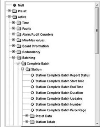
2..4 ID Data Tree

When selecting parameters and options in the Configurator software, the user will be presented with a tree structure for instance:

08/2013 - MA SUMMIT 8800 Vol2 R02 en

www.krohne.com

17

	GENERAL INFORMATION
02		SUMMIT 8800

Figure 1  Example ID Tree

This is referred to as the ID tree which, depending on its context, includes folders and several parameters:

2..4..1 Type of data

The rest of this chapter will explain the folders available, the type of selection within the folder and any other corresponding data.

Preset Data

Essential to the configuration of the flow computer. Typical data would be keypad values, operating limits, equation selection, calibration data for Turbines and Densitometers and Orifice plates.

This data would be present in a configuration report, and enables you to see what the flow computer is configured to do.

Used for validation and will form the Data Checksum (visible on the System Information Page). E.g., if a data checksum changes, the setup of the flow computer has changed and potentially calculating different results to what is expected.

Typically configured and left alone, only updated after validation e.g. every 6 month / 1 year.

Active Data

These values cover inputs to the flow computer. E.g., from GC, pressure & temperature transmitters, meters etc..

Also Values calculated in the flow computer. E.g., Flow rates, Z, Averages, Density etc..

Local Data

Data that an operator can change locally to perform maintenance tasks. E.g., turn individual transmitters off without generating alarms. Setting Maintenance mode or Proving Mode.

18

www.krohne.com

08/2013 - MA SUMMIT 8800 Vol2 R02 en

	GENERAL INFORMATION
SUMMIT 8800		02

Totals

Totals for the streams and station.

Contents of this folder are stored in the non-volatile RAM and are protected using the battery.

Custom

User defined variables.

Allows calculations, made in a LUA script, to be used in a configuration.

For details, see volume 3.

2..4..2 Colour codes

With each parameter and option, there are corresponding coloured dots that represent the access and status of the particular selection.

General ID tree

	Red Dot	Data is Read/Write and can be changed over Modbus.
	Yellow Dot	Data is Read-Only and cannot be changed over Modbus

Please note that it might be possible to change the values via the screen

90% of the data will be Read Only, but items such as Serial Gas Compositions, Time/Date, MF are commonly written over Modbus.

NOTE: Although the ID may be read/write, the security setting determines whether the ID indeed can be written.

Alarm Tree

The alarm tree is built of all the registers that hold alarm data. Alarm registers are 32-bit integers, where each bit represents a different alarm.

	Red Dot	Represents an accountable alarm visible on the alarm list.
	Dark Blue Dot	Represents a non-accountable alarm visible on the alarm list.
	Orange Dot	Represents a warning visible on the alarm list.
	Light Blue Dot	Represents a status alarm, not visible on the alarm list.
	Black/Grey Dot	Represents a hardor software fault alarm visible on the alarm list.

An example of typical usage would be the General Alarm Register. This is a 32 bit register that indicates up to 32 different alarms in the flow computer. This will contain Status Alarms, for example, 1 bit will indicate if there is a Pressure alarm or not. If the Pressure Status bit is set the user will know that there is a problem with the Pressure.

This should be sufficient information, however if it is not satisfactory, the user can look at the Pressure alarm, this contains 32 different alarms relating to the Pressure measurement, these would be Red Dots as they each can create an entry in the alarm list. By reading this register the user can view exactly what is wrong with the Pressure measurement.

The Light Blue Dots are generally an OR of several other dots. By reading the General register you can quickly see if the unit is healthy, more information can be provided by reading several more registers associated with that parameter.

08/2013 - MA SUMMIT 8800 Vol2 R02 en

www.krohne.com

19

	GENERAL INFORMATION
02		SUMMIT 8800

2..5 Specific Requirements for Meters and Volume Convertors

2..5..1 Numbering formats

The number formats used internally in the unit are generally IEEE Double Precision floating point numbers of 64 bit resolution.

It is accepted that such numbers will yield a resolution of better than 14 significant digits.

In the case of Totalisation of Gas, Volumes, Mass and Energy such numbers are always shown to a resolution of 8 digits before the decimal point and 4 after, i.e. 12 significant digits.

Depending upon the required significance of the lowest digit, these values can be scaled by a further multiplier.

2..5..2 Alarms

Each of the various modules that comprise the total operating software, are continuously monitored for correct operation. Depending upon the configuration, the flow computer will complete its allocated tasks within the configured cycle time, 250mS, 500mS or 1 second. Failure to complete the tasks within the time will force the module to complete, and where appropriate, a substitute value issued together with an alarm indication.

For example, if a Calculation fails to complete correctly then a result of 1 or similar will be returned, which allows the unit to continue functioning whilst an accountable alarm is raised, indicating an internal problem.

2..5..3 Accountable alarm

When the value of any measurement item or communication to an associated device that is providing measurement item to the SUMMIT 8800 goes out of range, the flow computer will issue an Accountable Alarm.

When any calculation module or other item that in some way affects the ultimate calculation result goes outside its operating band, i.e. above Pressure Maximum or below Pressure minimum, then the SUMMIT 8800 will issue an Accountable Alarm.

When the SUMMIT 8800 issues an Accountable alarm a number of consequences will occur as follows:

Front panel accountable alarm will turn on and Flash.

Nature of accountable alarm will be shown on the top line of the alarm log. Alarm log will wait for user acknowledgement of alarm.

During the period of the alarm, main totalisation will occur on the alarm counters.

2..5..4 Optional consequences

Depending upon the configuration of the SUMMIT 8800 the following optional Consequences will also occur:

An Entry will be made in the Audit Log, with Time and Date of occurrence.

The “Used” value of the Parameter in Alarm will be substituted by an alternative value, either from an alternative measurement source that is in range, or from a pre-set value.

A digital Alarm output will indicate an Alarm condition.

20

www.krohne.com

08/2013 - MA SUMMIT 8800 Vol2 R02 en

	METERING PRINCIPLES
SUMMIT 8800		03

In this Chapter the different meter technologies supported by the SUMMIT 8800 and the need for correction and normalization is described. Each of these technologies has its own particularities which are important to know when configuring the flow computer.

3..1 Pulse based meters: e..g.. turbine/ positive displacement / rotary meter

This method stems from the time when rotating meters where used, such as turbine meters and rotary (Positive displacement) meters.

Figure 2  Turbine and rotary meter

A turbine meter is basically a fan in a tube. The gas makes the fan rotate and the rotations are recorded in an index on top of the meter. A positive displacement or rotary meter consists of two tighly coupled impellers which together create a moving chamber of gas. The rotation of the impellers drive an index.

A contact switch is operated by the rotating meter. The result is that the periodic closure of the switch is directly related to the amount of gas going through the meter. Depending on the location of the switch there are:

HF pulses or high frequency pulses

•The switch can be mounted just above the turbine blades. This switch is closing at the higher rate than the meter rotates (typically up to 5000 Hz). The ratio between the two is called “blade ratio”.

MF pulses or medium frequency pulses

•The switch mounted on the primary axes, so this switch is closing every turn of the meter. This results in a medium frequency pulse (typically up to 500 Hz)

LF pulses or low frequency pulses

•For low cost meters the switch can be mounted in the index after a gear resulting in slow pulsing switches and in a low accuracy measurement (typically below 50 Hz)

A problem with this method is that the switches do not always close 100% reliable. This is particularly true for the HF pulses as non-contact switches are used. This means that we can have missing pulses. Also too many pulses can occur, e.g. when interference occurs with the high frequency wires or due to thunder storms. The solution is to have dual pulses and check the relation between the two.

It may also be that a turbine blade may break off resulting in the wrong measurement. There is therefore a need for diagnostics. Several solutions have been implemented:

•The dual pulse method with a 90° angle between the two. This allows for diagnostics and even corrections for missing pulses. An API classification level A to E is available (see below) for this.

•A second pulse from a turbine wheel with different blade angle.

08/2013 - MA SUMMIT 8800 Vol2 R02 en

www.krohne.com

21

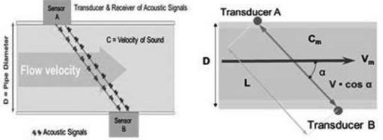
	METERING PRINCIPLES
03		SUMMIT 8800

•A second lower frequency pulse, so a combination of HF with MF or LF. Off course the frequency ratio or blade ratio between the two pulses must be given.

API has a classification on the quality actions taken on the pulses:

API level E is achieved solely by correctly applied	Basically a non-issue for flow computers
transmission systems, criteria and recommended
installed apparatus of good quality.
API level D system consists of manual error	This means: Only 1 pulse is needed on the flow
monitoring at methods of comparison, as used in	computer.
Levels A through D.
API level C consists of automatic error monitoring	This means: two pulses must be installed: the
for number, frequency, phase, and sequence and	meter pulse and monitor pulse, which may be of
error indication at specified intervals.	different frequency (see frequency ratio)
API level B consists of continuous monitoring, with	This means two pulses of the same frequency
an error indication under all circumstances when	must be installed: the meter and monitor pulse.
impaired pulses occur.
API level A: consists of continuous verification and	The major issue here is; the flow computer has
correction given by the comparator.	to correct when a wrong pulse occurs. This is
	quite advanced and is fully implemented in the
	SUMMIT.

Nowadays more and more electronics is incorporated into the meters, such as in ultrasonic and Coriolis meters. These meters normally emulate two high frequency pulses, to make them look the same as rotating meters from the installation standpoint. The flow is calculated and a special pulse output is driven by the processor. Although the need for a second output pulse is diminished, most meters still carry them. API Level A is not really required.

There are also meters with smart indexes. Here the indexes values itself can be read by the flow computer. The advantage is that the totals on the meters index are identical to the flow computer totals. Also, if the flow computer is replaced, the total will be automatically read. The communication is then digital and can be read via the serial port.

3..2 Ultrasonic meters

Ultrasonic meters are based on Transit Time Measurement of high frequency acoustic signals. These signals are transmitted and received along a diagonal measuring path.

A sound wave going downstream with the flow travels faster than a sound wave going upstream against the flow. The difference in transit time is directly proportional to the flow velocity of

the liquid or gas. This can be compared with the speed a canoe travels upstream compared to downstream.

Figure 3  Ultrasonic measurement principle

22

www.krohne.com

08/2013 - MA SUMMIT 8800 Vol2 R02 en

	METERING PRINCIPLES
SUMMIT 8800		03

Mathematically, the time to transmit from a to b and back depends on the distance (L) between the two transducers, the speeds of the medium (v) and sound (c) plus the angle of the path (α) as follows:

Equation 1  Ultrasonic measurement formulae

With the velocity of the gas and the area of the pipe, the volume flow rate can be calculated.

The problem is however that the oil or gas is not always equally distributed through the pipe. The flow normally is faster in the centre than in at the pipe and has a certain profile depending on turbulent or laminar flow. So you do need the proper average velocity over the complete pipe. With single beam meters, such as clamp-on meters, the accuracy is therefore very limited. That is why the medium must be measured at different locations in the pipe. The trick is to best estimate the profile/ the average flow. All manufacturers come up with different arrangements in multi-path meters.

The output of ultrasonic meters is normally a combination of a dual pulse and a serial link.

•The dual pulse is generated by the electronics to emulate a turbine meter but does not provide its diagnostics.

•The serial link has typically a modbus protocol specific to the manufacturer, but for Instromet there is also the proprietary “Instromet protocol”. This serial protocol carries the flow rate, but also meter diagnostics. For that reason in many cases both links are used at the same time.

Each manufacturer has its own set of diagnostics. Typical diagnostics are:

•The amplification needed to send a signal between the transducers, both upand downstream

•The signal to noise ratio at each transmitter

•The speed of sound measured by each path or ratio’s between them

•An indication of the type of flow profile

For gas there is an interesting additional diagnostics which is the calculated against the measured speed of sound based on AGA 10. The meter calculates besides the speed of the gas also the speed of sound. AGA 10 gives the formula from which the speed of sound can be calculated from the composition, the temperature and the pressure. Off course the measured and calculated speed of sound should be equal. If not one of the variables (meter, chromatograph or P or T) must be wrong or badly calibrated. This is therefore a perfect over all metering system check.

3..3 Differential pressure (dP) meters: e..g.. orifice, venturi and cone meter

Differential pressure flowmeters use the Bernoulli’s rule to measure the volume flow of gas or liquid in a pipe. They use a restriction in a pipe to measure the volume as it creates a differ-

ence in pressure before and after the restriction. The pressure difference (∆p) increases as flow increases.

08/2013 - MA SUMMIT 8800 Vol2 R02 en

www.krohne.com

23

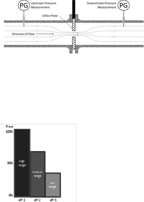
	METERING PRINCIPLES
03		SUMMIT 8800

Figure 4  DP measurement principles

The shape of the restriction is determines the type of meter: orifice, V-cone venture or nozzle (see later paragraphs). For each type there are several parameters that will be required to successfully calculate the flow rate.

A single dP transmitter can used, but the problem is that a transmitter typically only has a 1:3 turndown ratio, so the accuracy for low flow is very limited. For that reason in custody transfer applications multiple dP transmitters with different ranges are used for one meter and the flow computer switches between them over depending on the flow.

The SUMMIT can handle 1 to 3 ranges:

Figure 5  Up to 3 dP ranges

dP 1 will always measure the high range. In case of multiple ranges, an automatic switch-over to dP 2 will occur to medium range if the flow decreases to the dP measurement range, optimizing the accuracy. If 3 ranges are available, dP 3 will kick in when the flow gets within its measurement range.

In the SUMMIT the switch-up and switch-down values for the dP may be given. They will be normally be different to have some hysteresis to prevent continues switch-up and –down when at the threshold.

In high end applications, where the accuracy is crucial, multiple dP transmitters per range can be used for the following reasons:

24

www.krohne.com

08/2013 - MA SUMMIT 8800 Vol2 R02 en

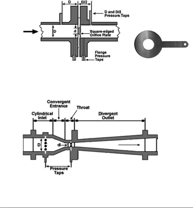
	METERING PRINCIPLES
SUMMIT 8800		03

•Accuracy: By averaging the transmitter values.

•Redundancy: If one transmitter fails, the other value may be used.

•Diagnostics: A warning can be given if there is a deviation between the transmitters.

For diagnostics 2 transmitters can be used, but it is not possible to determine which one is correct. For that reason 3 dP transmitters may be used.

The SUMMIT also can have 1 to 3 dP transmitters for 1 to 3 ranges, so 1 to 9 dP transmitters in total.

3..3..1 Orifice Plate

A flat circular plate with a hole, mounted inside the pipe that causes the fluid to push through a smaller diameter.

Figure 6  Orifice meter and plate

This is the most commonly used type of meter.

Classical venture or Herschel venturi

Consists of a tapering in the pipe.

Figure 7  Venturi tube layout

08/2013 - MA SUMMIT 8800 Vol2 R02 en

www.krohne.com

25

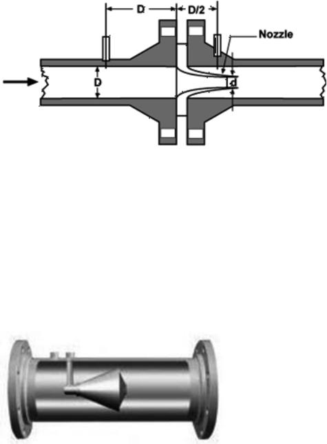
	METERING PRINCIPLES
03		SUMMIT 8800

3..3..2 Venturi nozzle

The venturi nozzle has a trumpet shape restriction ending up in the pipe..

Figure 8  Venturi Nozzle

The main advantage of the venturi nozzle is pressure recovery.

ISA 1932 nozzle

Typically used for high velocity, set by ISO 5167 to determine the flow of fluid.

Long radius nozzle

A variation of the ISA 1932 nozzle, with a convergent section as the ISA 1932 nozzle and divergent section as a classical venturi

Cone or V-cone meter

The shape of the cone is to stable the flow profile in order to accurately measure the fluid regardless of flow properties.

Figure 9  V-cone meter

3..4 Coriolis meters

The Coriolis effect is the deflection of a fluid by a rotating effect. If the rotation is clockwise, the deflection is to the left, if counter-clockwise, the deflection is to the right.

Coriolis meters use a vibrating meter tube to generate the rotating effect and measure the deflection to calculate the mass passing through the meter.

26

www.krohne.com

08/2013 - MA SUMMIT 8800 Vol2 R02 en

	METERING PRINCIPLES
SUMMIT 8800		03

Figure 10  Coriolis meter flow principle

A tube with a fluid is brought into a sine waveform vibration. The eigen frequency with which this occurs is directly dependent on the density of the fluid. If the fluid is flowing, a phase shift of the vibration will occur between the inlet and outlet of the tube. This phase shift is a measure of the velocity with which the fluid passes through the pipe.

Traditional Coriolis meters have a bent tube to maximize the Coriolis effect. With more advanced electronics nowadays there is also straight tube Coriolis meters (see drawing).

Coriolis meters determine the mass flow, but can also determine the density. Most Coriolis meters will also calculate the volume flow using internal temperature and pressure, but it is recommended to use external measurements because of accuracy.

Coriolis meters typically have a dual pulse output mostly with the choice to have mass or volume flow rate, where mass flow rate is more accurate. Because of the fact that also density, pressure and temperature are available, most meters have also the option for a serial (modus) output, or a (multi-variable) Hart output.

08/2013 - MA SUMMIT 8800 Vol2 R02 en

www.krohne.com

27

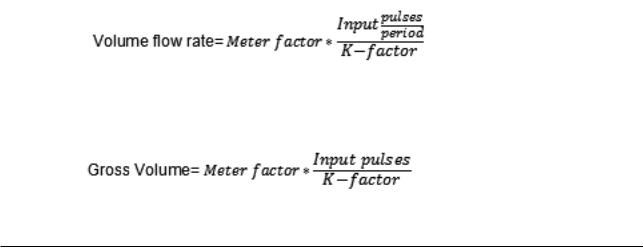
	METERING PRINCIPLES
03		SUMMIT 8800

3..5 Meter corrections

3..5..1 Gas & steam

The meter provides a number of pulses/s. We would like to know the Volume flow rate e.g. m3/s. For this need:

Pulse factor or impulse factor or meter factor

The factor provided by the manufacturer of the meter giving the number of pulses per volume of gas e.g. Pulses/m3. This assumes a linear meter. This is configured in the meter section.

Linearisation/ error Curve

The errors in % obtained during calibration of a meter which are the corrections needed to linearise the meter. So for each flow rate a different error is used. In between the given flow rates a linear interpolation is used. For flow outside the operating range, extrapolation is used, except when MID is chosen, then the error is fixed, and low and high flow is used.

Volume flow rate= Pulses per period*(1-Error)

Gross Volume= Pulses*(1-Error)

3..5..2 Liquid

The meter provides a number of pulses/s. We would like to know the Volume flow rate e.g. gallons/s. For this there are three important corrections for the meter possible:

K-factor

The factor provided by the manufacturer of the meter or as a result of proving which is the number of pulses per volume of fluid e.g. Pulses/gallon.

For a linear meter only one factor can be given.

In case that the meter is not linear then a K-factor curve can be used. In this These factors are obtained during calibration or prove of a meter which are the corrections needed to linearise the meter. This is expressed by a variation of the K-factor over the specified flow range. So for each flow rate a different K-factor is used. In between the given flow rates a linear interpolation is used. For flow above maximum extrapolation is used.

Meter factor

The factor determined during proving to correct a fluid flowmeter for the ambient conditions by shifting its curve. The factor is used to compensate for such conditions as liquid temperature change and pressure shrinkage and is meter and product dependent. The meter factor should be close to1.

Equation 2  Volume calculation with MF

Equation 3  Gross volume calculation with MF

28 www.krohne.com 08/2013 - MA SUMMIT 8800 Vol2 R02 en

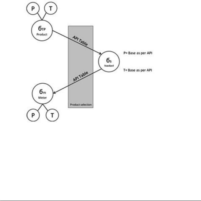
	METERING PRINCIPLES
SUMMIT 8800		03

3..6 Liquid normalisation

As with gas also oil flow is measured by meters using a variety of different measurement principles, most based on volume flow, some based on mass flow. Examples are turbine meters, orifice meters, Coriolis meters and ultrasonic meters. In all cases the line flow is measured. The problem with this is that two measurements in the same pipe cannot be compared, due to difference in temperature, (to a lesser extend) pressure and possibly the type of product. This also means that billing of the oil will not be possible as no fixed tariff can be applied.

For this reason a flow computer is used to “normalize” the oil flow to standard (or base) conditions, such as:

Temperature	15 or 20 oC or 60 oF
Pressure	1.01325 bar or 14.73 psi

So from the input density, the standard density is calculated by correcting for pressure and density. Then, from the standard density, the meter density is calculated, by again correcting for pressure and density.

Figure 11  Density calculations for oil

08/2013 - MA SUMMIT 8800 Vol2 R02 en

www.krohne.com

29

0, 15 or 20 °C or 60 °F 1.01325 bar or 14.73 psi

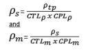
	METERING PRINCIPLES
03		SUMMIT 8800

The following formula applies:

Where
ρm	Line density of the liquid at metering conditions in kg/m3 or lbs/ft3
ρtp	Line density of the liquid corrected for temperature and pressure in kg/m3 or lbs/ft3
ρs Standard Density of Liquid in kg/m3 or lbs/ft3
CTLρ :	Temperature correction factor density at density test point
CPLρ :	Pressure correction factor density at density test point
CTLm :	Temperature correction factor at the meter
CPLm :	Pressure correction factor at the meter

Several different calculations, depending on the type of product, are available to determine the correction factors.

3..6..1 Mass and energy

The mass and energy can be calculated from the volume (or the volume from the mass) using:

Mass flow rate:	qm= qbc* ρm
Energy flow rate:	qe= qn* Hs

Where Hs is the heating value. Two types can be used:

•The superior heating value, also known as higher heating value or higher calorific value or gross calorific value represents the heat released when a unit mass or volume of a material at 1 bar pressure and 25 °C is completely combusted and the combustion products are brought back to the starting pressure and temperature.

•The inferior heating value, also known as lower heating value or lower calorific value or net calorific value. This quantity assumes that the water produced by combustion remains in the vapour phase in the exhaust, and is lower than the gross calorific value by the latent heat of condensation joules/gram) of water at 25°C multiplied by the concentration of water in the material (expressed as grams/gram of fuel). For most common fuels, the net calorific value is about 10% less than the gross calorific value.

3..7 Gas normalisation

Gas is a compressible fluid, due to this fact the reference conditions (P base and T base) on which the volume is calculated has to be given, which are normally contractually agreed.

Gas flow is measured by meters using a variety of different measurement principles, most based on volume flow, some based on mass flow. Examples are turbine meters, orifice meters, Coriolis meters and ultrasonic meters. In all cases the line flow is measured. The problem with this is that two measurements in the same pipe cannot be compared, due to difference in temperature, pressure and possibly the composition of the product. This also means that billing of the gas will not be possible as no fixed tariff can be applied.

For this reason a flow computer is used to “normalize” the gas flow to standard (or base) conditions, such as:

Temperature Pressure

30

www.krohne.com

08/2013 - MA SUMMIT 8800 Vol2 R02 en