


Remote programming and measuring uncommon RTDs with the Fluke 726
Application Note
RTD Temperature Curves
RTD’s take advantage of a natural property of metals, namely that a metal’s resistance increases with temperature. An RTD is a precisely manufactured metal wire or film, and by measuring its resistance we can derive its temperature.
Resistance of an RTD is a function of the length and cross sectional area of the wire or film used to make it, and the resistivity of its metal. Resistivity is a characteristic of a metal’s chemical makeup. Most RTD’s are made of platinum, nickel, or copper. The alloy of the platinum or copper must be tightly controlled to produce precise resistivity. International standards like IEC 60751 and ASTM 1137 define the geometry and resistivity of standard RTD’s. RTD manufacturers work to build their product to meet these standards.
In addition to defining the physical parameters of standard RTD’s, international standards also define equations and constants used to convert resistance readings to temperature. Over a limited range the relationship between temperature and resistance is approximately linear, and you can convert temperature to resistance using Equation 1.
Using custom RTD temperature constants
The Fluke 726 Multifunction Process Calibrator can measure temperature with most common resistance temperature detectors (RTD’s). But what about the many “legacy” non-standard RTD’s still in use, as well as standard RTDs that have been specially calibrated? The 726 allows you to enter custom RTD constants so you can measure any RTD for which you have the constants. You can also use custom constants to take advantage of the Fluke 726 ability to measure with 0.01° resolutions by coupling it with a characterized RTD. This application note explains how
to use the 726 to measure non-standard or characterized RTD’s. It covers the basic theory of RTD conversion formulas and shows how to load custom constants into the Fluke 726 using a Windows PC with an RS-232 serial port.
Equation 1: Rt = R0 (1 + αt)
Where: t is the temperature of the sensor R0 is the resistance at 0 °C.
α is a constant slope that describes resistance change per degree C.
Rt is the resistance at temperature t, in degrees C.
Using this simple linear equation delivers fairly good results, especially at temperatures between 0 and 100 °C. To extend the range of the RTD and to get more precision, IEC and ASTM standards specify a more complex polynomial that fine-tunes the resistance-temperature relationship. One form of that equation is given here as Equation 2. The RTD standards also specify values for the constants R0, A, B, C. (The C constant is only used for temperatures less than 0 °C.)
F r o m t h e F l u k e D i g i t a l L i b r a r y @ w w w . f l u k e . c o m / l i b r a r y
|
300.000 |
|
|
|
|
|
|
|
|
|
|
|
|
|
|
|
280.000 |
|
|
|
|
|
|
|
|
|
|
|
|
|
|
(Ohms) |
260.000 |
|
|
|
|
|
|
|
|
|
|
|
|
||
|
|
|
|
|
|
|
|
Resistance |
240.000 |
|
|
|
|
|
Rt polynomial |
|
|
|
|
|
Rt linear |
||
|
|
|
|
|
|
||
|
220.000 |
|
|
|
|
|
|
|
|
|
|
|
|
|
|
|
|
|
|
|
|
|
|
|
200.000 |
|
|
|
|
|
|
|
|
|
|
|
|
|
180.000 |
|
|
|
|
|
|
200 |
250 |
300 |
350 |
400 |
450 |
500 |
Temperature (C)
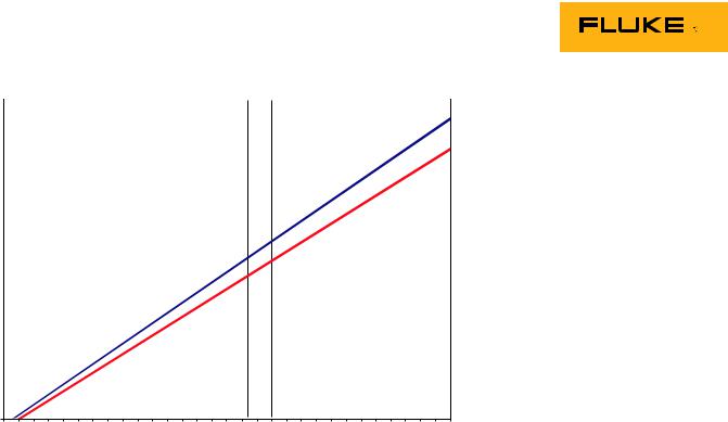
Figure 1. RTD Curves.
Equation 2: Rt = R0 [1 + At + Bt2 + C(t — 100)t3]
Figure 1 shows the difference between temperature values produced by the linear equation and the polynomial between 200 and 500 °C. Note that at 240 ohms, the polynomial curve of Equation 2 gives a more accurate temperature 16 °C higher than the linear equation.
The Fluke 726 uses the polynomial in Equation 2 and it has built-in constants to support most common RTD’s. Standard RTD’s supported by the Fluke 726 are shown in Table 1.
Older or specialized equipment may use nonstandard RTDs. Well-equipped standards labs can improve the accuracy of an RTD by adjusting the constants to suit a particular sensor. The Fluke 726 allows you to check less common RTD’s or take advantage of RTD’s that have been characterized, by specifying your own values for R0, A, B and C.
For example, for the common Pt 385 RTD with 100 Ω resistance at 0 °C, the constants are:
R0 = 100 Ω
A= 3.9083 x 10⁻³
B= -5.775 x 10⁻⁷
C= -4.183 x 10⁻¹²
Note: Instruments installed before and up to the early 1990s used a slightly different temperature scale (IPTS-68) than newer instruments (ITS-90). When a calibrator using ITS-90 RTD curves is used to calibrate an instrument using IPTS-68 errors will result. The errors are extremely small at room temperature and increase to a maximum of 0.36 °C at 760 °C.
RTD Type |
Reference R0, |
Metal |
α |
Range |
|
|
|
Ohms |
|
Ω/Ω/°C |
°C |
Pt 100 |
(3916) |
100 |
Platinum |
0.003916 |
-200 to 630 |
Pt 100 |
(385)* |
100 |
Platinum |
0.00385 |
-200 to 800 |
|
|
|
|
|
|
Pt 200 (385) |
200 |
Platinum |
0.00385 |
-200 to 630 |
|
Pt 500 (385) |
500 |
Platinum |
0.00385 |
-200 to 630 |
|
Pt 1000 (385) |
1000 |
Platinum |
0.00385 |
-200 to 630 |
|
|
|
|
|
|
|
Pt 100 |
(3926) |
100 |
Platinum |
0.003926 |
-200 to 630 |
Ni 120 (672) |
120 |
Nickel |
0.00672 |
-80 to 260 |
|
Cu 10 (42) |
10 |
Copper |
0.0042 |
-10 to 250 |
|
Table 1: Standard RTDs types included in the Fluke 726.
Pt 100 (385) is the IEC and ASTM standard.
Another common form of Equation 2, the Callendar Van Dusen or CVD, uses the constants α, δ, and β. This alternative form is directly derived from Equation 1 and uses the same constant α. And even though the two polynomials produce the same results, the constants are different. The Fluke 726 uses the constants A, B, and C. If you know the α, δ, and β constants for an RTD you can convert them to A, B, C constants by using Equations 3, 4 and 5.
Equation 3: A = α + α . δ
100
Equation 4: B = — α . δ
1002
Equation 5: C = — α . β
1004
2 Fluke Corporation Measuring uncommon RTDs with the Fluke 726

Loading custom RTD constants into the Fluke 726
Setting up communications
Figure 2.
The Fluke 700SC Serial Interface Cable (PN 667425) is used to communicate with the Fluke 726. The serial cable connects to the round multipin connector at the top of the 726 and to a 9-pin serial port on your PC. The serial cable can only interface with one instrument or module at a time.
After connecting the cable, make sure the 726 is turned on. Call up the Windows HyperTerminal Program. It is usually listed in the Windows Start Programs menu under Accessories, Communications. The HyperTerminal program will ask you to set up a file name to store your communication settings. You can select any icon and click OK to continue.
Figure 3.
A second dialog box, “Connect To”, will pop up. Skip down to the bottom, where it says “Connect Using:” Select the COM port you connected to the 726.
Figure 4.
Next, a COM Properties box will come up. Set baud rate (9600 in Figure 4), data bits, parity, stop bits and flow control as shown in the Figure 4. Once your settings match Figure 4, click OK to continue.
Figure 5.
To make it easier to read the commands and responses, you can make some adjustments to the way the HyperTerminal program treats screen text. Under the File menu select Properties and click on the Settings tab. Click on the button labeled ASCII Setup. You will see a dialog like the one shown in Figure 5. Match the settings shown in the figure. Note that adding the 200 ms line delay makes it possible to send short scripts to the 726. More on this later.
To test the connection, type: *idn?
After you hit Enter, the 726 should respond with “FLUKE,726,0,X.X” where X.X is the version of the firmware in the instrument.
3 Fluke Corporation Measuring uncommon RTDs with the Fluke 726
 Loading...