

Page 1

TI-82
GRAPHING CALCULATOR
GUIDEBOOK
TI-GRAPH LINK, Calculator-Based Laboratory, CBL, CBL 2, Calculator-Based Ranger,
CBR, Constant Memory, Automatic Power Down, APD, and EOS are trademarks of
Texas Instruments Incorporated.
Macintosh is a registered trademark of Apple Computer, Inc.
© 1993, 2000, 2001 Texas Instruments Incorporated.
Page 2

Important
Texas Instruments makes no warranty, either expressed or implied,
including but not limited to any implied warranties of merchantability and
fitness for a particular purpose, regarding any programs or book materials
and makes such materials available solely on an “as-is” basis.
In no event shall Texas Instruments be liable to anyone for special,
collateral, incidental, or consequential damages in connection with or
arising out of the purchase or use of these materials, and the sole and
exclusive liability of Texas Instruments, regardless of the form of action,
shall not exceed the purchase price of this equipment. Moreover, Texas
Instruments shall not be liable for any claim of any kind whatsoever against
the use of these materials by any other party.
US FCC Information Concerning Radio Frequency Interference
This equipment has been tested and found to comply with the limits for a Class
B digital device, pursuant to Part 15 of the FCC rules. These limits are designed
to provide reasonable protection against harmful interference in a residential
installation. This equipment generates, uses, and can radiate radio frequency
energy and, if not installed and used in accordance with the instructions, may
cause harmful interference with radio communications. However, there is no
guarantee that interference will not occur in a particular installation.
If this equipment does cause harmful interference to radio or television
reception, which can be determined by turning the equipment off and on, you
can try to correct the interference by one or more of the following measures:
Reorient or relocate the receiving antenna.
•
Increase the separation between the equipment and receiver.
•
Connect the equipment into an outlet on a circuit different from that to
•
which the receiver is connected.
Consult the dealer or an experienced radio/television technician for help.
•
Caution:
approved by Texas Instruments may void your authority to operate the
equipment.
Any changes or modifications to this equipment not expressly
Page 3

Table of Contents
This manual describes how to use the TI.82 Graphing Calculator. Getting Started
gives a quick overview of its features. The first chapter gives general instructions
on operating the TI.82. Other chapters describe its interactive features. The
applications in Chapter 14 show how to use these features together.
Using this Guidebook Effectively
Glossary
Getting Started: Do This First!
TI.82 Menus
First Steps
.....................................
..................................
...................................
Entering a Calculation: Compound Interest
Defining a Function: Box with Lid
Defining a Table of Values
Zooming In on the Table
Changing the Viewing
Displaying and Tracing the Graph
Zooming In on the Graph
Finding the Calculated Maximum
Other Features
Chapter 1: Operating the TI.82
Turning the TI.82 On and Off
Setting the Display Contrast
The Display
..................................
Entering Expressions and Instructions
TI.82 Edit Keys
Setting Modes
TI.82 Modes
..................................
Variable Names
Storing and Recalling Variable Values
....................................
Last Entry
Last Answer
TI.82 Menus
VARS
..................................
..................................
and
Y-VARS
EOSé (Equation Operating System)
Error Conditions
...................
............
..................
........................
..........................
....................
WINDOW
...................
.........................
...................
................................
......................
.......................
...............
................................
.................................
................................
................
Menus
........................
.................
...............................
viii
x
2
3
4
6
7
8
10
11
12
13
14
1-2
1-3
1-4
1-6
1-8
1-9
1-10
1-12
1-13
1-14
1-16
1-17
1-19
1-20
1-22
Introduction iii
Page 4

Chapter 2: Math, Angle, and Test Operations
Getting Started: Lottery Chances
Keyboard Math Operations
MATH MATH
MATH NUM
MATH HYP
MATH PRB
ANGLE
TEST TEST
TEST LOGIC
Chapter 3: Function Graphing
Operations
(Number) Operations
(Hyperbolic) Operations
(Probability) Operations
Operations
(Relational) Operations
(Boolean) Operations
.........................
.............................
Getting Started: Graphing a Circle
Defining a Graph
Setting Graph Modes
Defining Functions in the
Selecting Functions
Defining the Viewing
Setting
WINDOW FORMAT
Displaying a Graph
...............................
............................
Y=
.............................
WINDOW
........................
.............................
Exploring a Graph with the Free-Moving Cursor
Exploring a Graph with
Exploring a Graph with
Using
ZOOM MEMORY
Setting
ZOOM FACTORS
Using
Chapter 4: Parametric Graphing
(Calculate) Operations
CALC
TRACE
ZOOM
..........................
.........................
Getting Started: Path of a Ball
Defining and Displaying a Parametric Graph
Exploring a Parametric Graph
...................
.......................
..................
.................
.................
.................
.................
..................
...................
List
....................
........
....................
.....................
.................
.....................
...........
.....................
2-2
2-3
2-5
2-9
2-11
2-12
2-13
2-15
2-16
3-2
3-3
3-4
3-5
3-7
3-8
3-10
3-11
3-13
3-14
3-16
3-19
3-21
3-22
4-2
4-3
4-6
Chapter 5: Polar Graphing
Getting Started: Polar Rose
Defining and Displaying a Polar Graph
Exploring a Polar Graph
iv Introduction
.......................
...............
.........................
5-2
5-3
5-6
Page 5

Chapter 6: Sequence Graphing
Getting Started: Forest and Trees
Defining and Displaying a Sequence Graph
Exploring a Sequence Graph
Chapter 7: Tables
Getting Started: Roots of a Function
Defining the Variables
Defining the Dependent Variable
Displaying the Table
Chapter 8: DRAW Operations
Getting Started: Shading a Graph
DRAW DRAW
Menu
Drawing Lines
Drawing Horizontal and Vertical Lines
Drawing Tangent Lines
Drawing Functions and Inverses
Shading Areas on a Graph
Drawing Circles
Placing Text on a Graph
Using
to Draw on a Graph
Pen
Drawing Points
Drawing Pixels
Storing and Recalling Graph Pictures
Storing and Recalling Graph Databases
Clearing a Drawing
...................
............
......................
.................
...........................
...................
............................
...................
............................
................................
...............
..........................
...................
........................
...............................
.........................
.....................
................................
................................
................
...............
.............................
6-2
6-3
6-6
7-2
7-3
7-4
7-5
8-2
8-3
8-4
8-5
8-6
8-7
8-8
8-9
8-10
8-11
8-12
8-13
8-14
8-15
8-16
Chapter 9: Split Screen
Getting Started: Polynomial Coefficients
Using Split Screen
..............
..............................
Introduction v
9-2
9-3
Page 6

Chapter 10: Matrices
Getting Started: Systems of Linear Equations
Defining a Matrix
Viewing Matrix Elements
Editing Matrix Elements
About Matrices
Matrix Math Functions
MATRIX MATH
Chapter 11: Lists
Getting Started: Generating Sequences
About Lists
LIST OPS
LIST MATH
Chapter 12: Statistics
Getting Started: Building Height and City Size
Setting Up a Statistical Analysis
Viewing List Elements
Editing List Elements
STAT EDIT
Statistical Analysis
Statistical Variables
Types of Statistical Analysis
Statistical Analysis in a Program
Statistical Plotting
Statistical Plotting in a Program
..........
..............................
.........................
.........................
................................
..........................
Operations
........................
...............
...................................
Operations
Operations
...........................
..........................
..........
....................
...........................
...........................
...............................
Menu
.............................
.............................
.......................
...................
..............................
....................
10-2
10-4
10-5
10-6
10-8
10-10
10-12
11-2
11-3
11-6
11-9
12-2
12-9
12-10
12-11
12-12
12-13
12-14
12-15
12-17
12-18
12-22
Chapter 13: Programming
Getting Started: Family of Curves
About Programs
Creating and Executing Programs
Editing Programs
PRGM CTL
PRGM I/O
Calling Other Programs
vi Introduction
...................
...............................
..................
..............................
(Control) Instructions
(Input/Output) Instructions
..................
...............
..........................
13-2
13-4
13-5
13-6
13-7
13-15
13-18
Page 7

Chapter 14: Applications
Left-Brain, Right-Brain Test Results
Speeding Tickets
Buying a Car, Now or Later?
Graphing Inequalities
Solving a System of Nonlinear Equations
Program: Sierpinski Triangle
Cobweb Attractors
Program: Guess the Coefficients
The Unit Circle and Trigonometric Curves
Ferris Wheel Problem
Reservoir Problem
Predator-Prey Model
Fundamental Theorem of Calculus
Finding the Area between Curves
Chapter 15: Memory Management
Checking Available Memory
Deleting Items from Memory
Resetting the TI.82
Chapter 16: Communication Link
Getting Started: Sending Variables
TI.82
...................................
LINK
Selecting Items to Send
Transmitting Items
Receiving Items
Backing Up Memory
.................
...............................
......................
...........................
.............
......................
.............................
...................
............
...........................
.............................
............................
..................
...................
.......................
......................
.............................
..................
..........................
.............................
...............................
............................
14-2
14-4
14-5
14-6
14-7
14-8
14-9
14-10
14-11
14-12
14-14
14-16
14-18
14-20
15-2
15-3
15-4
16-2
16-3
16-4
16-6
16-7
16-8
Appendix A: Tables
Tables of Functions and Instructions
Menu Map
...................................
Table of System Variables
Appendix B: Reference Information
Battery Information
In Case of Difficulty
Accuracy Information
Error Conditions
...............................
Service and Support Information
Warranty Information
Index
................
........................
.............................
............................
...........................
...................
...........................
Introduction vii
A-2
A-22
A-28
B-2
B-4
B-5
B-7
B-11
B-12
Page 8

Using this Guidebook Effectively
The structure of the TI.82 guidebook and the design of its pages can help you
find the information you need quickly. Consistent presentation techniques are
used throughout to make the guidebook easy to use.
Structure of the Guidebook
The guidebook contains sections that teach you how to use the calculator.
¦
Getting Started is a fast-paced keystroke-by-keystroke introduction.
¦
Chapter 1 describes general operation and lays the foundation for
Chapters 2 through 13, which describe specific functional areas of the
TI.82. Each begins with a brief Getting Started introduction.
¦
Chapter 14 contains application examples that incorporate features
from different functional areas of the calculator. These examples can
help you see how different functional areas work together to
accomplish meaningful tasks.
¦
Chapter 15 describes memory management and Chapter 16 describes
the communications link.
Page-Design Conventions
When possible, units of information are presented on a single page or on
two facing pages. Several page-design elements help you find information
quickly.
¦
Page headings—The descriptive heading at the top of the page or twopage unit identifies the subject of the unit.
¦
General text—Just below the page heading, a short section of bold
text provides general information about the subject covered in the unit.
¦
Left-column subheadings—Each subheading identifies a specific
topic or task related to the page or unit subject.
¦
Specific text—The text to the right of a subheading presents detailed
information about that specific topic or task. The information may be
presented as paragraphs, numbered procedures, bulleted lists, or
illustrations.
¦
Page “footers”—The bottom of each page shows the chapter name,
chapter number, and page number.
viii Introduction
Page 9

Information-Mapping Conventions
Several conventions are used to present information concisely and in an
easily referenced format.
¦
Numbered procedures—A procedure is a sequence of steps that
performs a task. In this guidebook, each step is numbered in the order
in which it is performed. No other text in the guidebook is numbered;
therefore, when you see numbered text, you know you must perform
the steps sequentially.
¦
“Bulleted” lists—If several items have equal importance, or if you
may choose one of several alternative actions, this guidebook precedes
each item with a “bullet” (
¦
Tables and charts—Sets of related information are presented in tables
or charts for quick reference.
¦
Keystroke Examples—The Getting Started examples provide
keystroke-by-keystroke instructions, as do examples identified with a
.
Reference Aids
Several techniques have been used to help you look up specific information
when you need it. These include:
¦
A chapter table of contents on the first page of each chapter, as well as
the full table of contents at the front of the guidebook.
¦
A glossary at the end of this section, defining important terms used
throughout the guidebook.
¦
An alphabetical table of functions and instructions in Appendix A,
showing their correct formats, how to access them, and page references
for more information.
¦
Information about system variables in Appendix A.
¦
A table of error messages in Appendix B, showing the messages and
their meanings, with problem-handling information.
¦
An alphabetical index at the back of the guidebook, listing tasks and
topics you may need to look up.
¦
) to highlight it—like this list.
Introduction ix
Page 10

Glossary
v
v
This glossary provides definitions for important terms that are used throughout
this guidebook.
Expression
Function
Graph Database
Graph Picture
Home Screen
Instruction
List
Matrix
Menu Items
Pixel
Variable
An expression is a complete sequence of numbers, variables,
functions, and their arguments that can be evaluated to a single
answer.
A function, which may have arguments, returns a value and can
be used in an expression.
A function is also the expression entered in the
in graphing and
TABLE
.
editor used
Y=
A graph database is composed of the elements that define a
graph: functions in the
Y=
list,
MODE
settings, and
WINDOW
settings. They may be saved as a unit in a graph database to
recreate the graph later.
A picture is a saved image of a graph display, excluding cursor
coordinates, axis labels, tick marks, and prompts. It may be
superimposed on another graph.
The Home Screen is the primary screen of the TI.82, where
expressions can be entered and evaluated and instructions can
be entered and executed.
An instruction, which may have arguments, initiates an action.
Instructions are not valid in expressions.
A list is a set of values that the TI.82 can use for activities such
as graphing a family of curves, evaluating a function at multiple
alues, and entering statistical data.
A matrix is a two-dimensional array on which the TI.82 can
perform operations.
Menu items are shown on full-screen menus.
A pixel (picture element) is a square dot on the TI.82 display.
The TI.82 display is 96 pixels wide and 64 pixels high.
A variable is the name given to a location in memory in which a
alue, an expression, a list, a matrix, or another named item is
stored.
x Introduction
Page 11

Getting Started: Do This First!
Getting Started contains two keystroke-by-keystroke examples, an interest rate
problem and a volume problem, that introduce you to some principal operating
and graphing features of the TI.82. You will learn to use the TI.82 much more
quickly by completing both of these examples first.
Contents
TI.82 Menus
First Steps
Entering a Calculation: Compound Interest
Defining a Function: Box with Lid
Defining a Table of Values
Zooming In on the Table
Changing the Viewing
Displaying and Tracing the Graph
Zooming In on the Graph
Finding the Calculated Maximum
Other Features
................................
.................................
..........
................
......................
........................
..................
WINDOW
.................
.......................
.................
..............................
2
3
4
6
7
8
10
11
12
13
14
Getting Started 1
Page 12
TI-82 Menus
A
A
To leave the keyboard uncluttered, the TI.82 uses full-screen menus to access
many additional operations. The use of specific menus is described in the
appropriate chapters.
Displaying a Menu
When you press a key that accesses a menu, such
as
screen where you are working.
usually are returned to the screen where you were.
Moving from One Menu to Another
names of the menus appear on the top line. The
current menu is highlighted and the items in that
menu are displayed.
Use ~ or | to display a different menu.
Selecting an Item from a Menu
The number of the current item is highlighted. If
there are more than seven items on the menu, a
appears on the last line in place of the : (colon).
To select from a menu:
¦
¦
Leaving without Making a Selection
To leave a menu without making a selection:
¦
¦
¦
, that menu screen temporarily replaces the
fter you make a selection from a menu, you
menu key may access more than one menu. The
Use † and } to move the cursor to the item
and then press
Í
.
Press the number of the item.
ä
ã
QUIT
Press y
‘
Press
to return to the Home screen.
to return to the screen where you
were.
Select another screen or menu.
$
2 Getting Started
Page 13
First Steps
Before beginning these sample problems, follow the steps on this page to reset
the TI.82 to its factory settings. (Resetting the TI.82 erases all previously entered
data.) This ensures that following the keystrokes in this section produces the
illustrated actions.
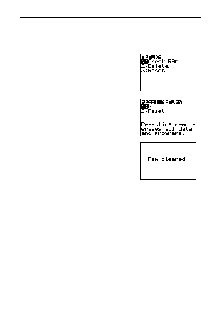
1. Press É to turn the calculator on.
2. Press and release y and then press Ã.
(Pressing y accesses the operation printed in
blue to the left above the next key that you
press.
The
3. Press 3 to select
The
is the
MEM
MEMORY
RESET MEMORY
2nd
menu is displayed.
Reset...
operation of Ã.)
.
menu is displayed.
4. Press 2 to select
. The calculator is reset.
Reset
5. After a reset, the display contrast is also reset. If
the screen is very dark or blank, you need to
adjust the display contrast. Press y and then
press and hold † (to make the display lighter)
or } (to make the display darker). You can
‘
press
to clear the display.
Getting Started 3
Page 14
Entering a Calculation: Compound Interest
Using trial and error, determine when an amount invested at 6% annual
compounded interest will double in value. The TI.82 displays up to 8 lines of 16
characters so you see an expression and its solution at the same time. You also
can store values to variables, enter multiple instructions on one line, and recall
previous entries.
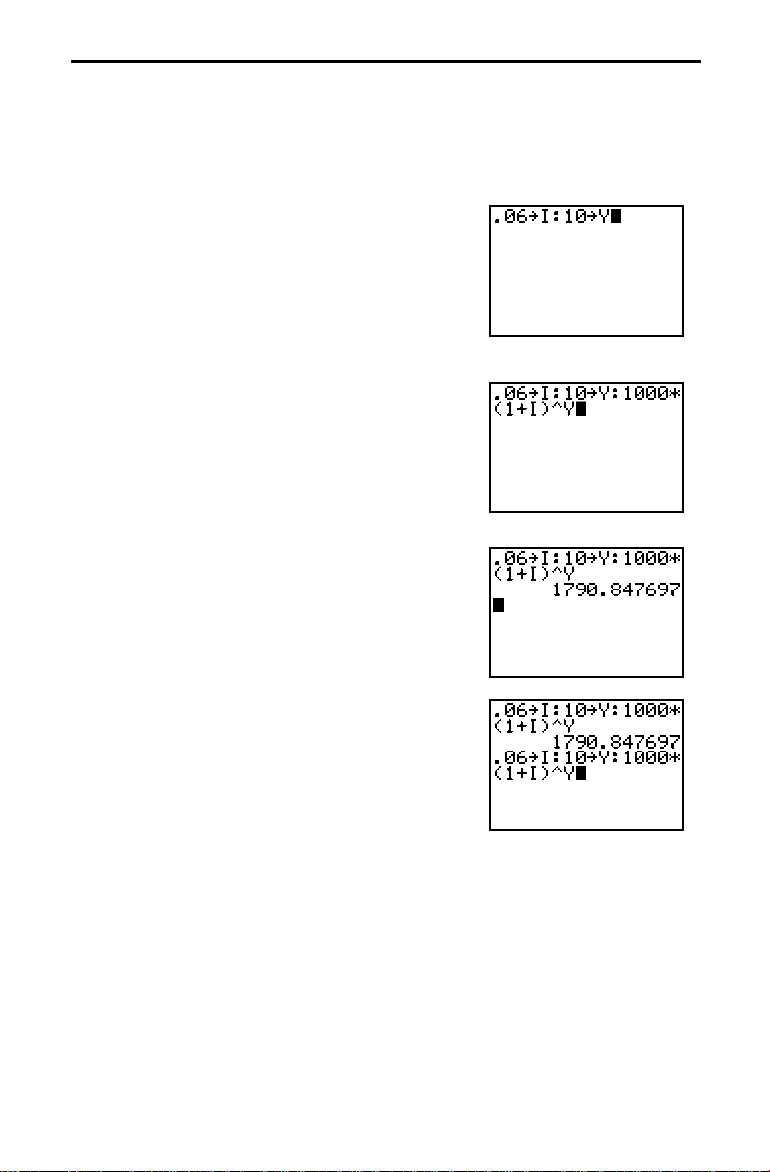
1. Press
.06
¿
ƒ
Z (annual interest rate) to
store the interest rate.
ã
ä
2. Press y
:
to enter more than one instruction
on a line.
3. For the first guess, compute the amount
available at the end of 10 years. Enter
ƒ
(years).
Y
ä
ã
:
4. Press y
, then enter the expression to
10
calculate the total amount available after
years at Z interest just as you would write it. Use
1000 as the amount. Press
ƒ
Z
¤ ›
Y.
1000
¯ £ 1 Ã
The entire problem is shown in the first two
lines of the display.
5. Press
Í
to evaluate the expression.
The answer is shown on the right side of the
display. The cursor is positioned on the next
line, ready for you to enter the next expression.
6. To save keystrokes, you can use
Last Entry
recall the last expression entered and then edit
it for a new calculation. Press y, followed by
ä
ã
ENTRY
(above
Í
).
The last calculated expression is shown on the
next line of the display.
¿
Y
ƒ
to
4 Getting Started
Page 15
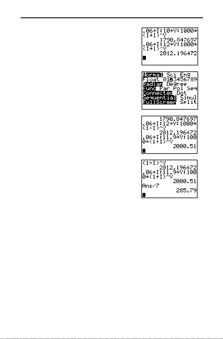
7. The next guess should be greater than 10
years. Make the next guess 12 years. Press
to move the cursor over the
to change 10 to 12. Press
, and then type
0
Í
to evaluate the
}
2
expression.
8. To display answers in a format more
appropriate for calculations involving money,
press z to display the
MODE
screen.
9. Press † ~ ~ ~ to position the cursor over the
2 and then press
Í
. This changes the
display format to two fixed decimal places.
ä
ã
QUIT
10. Press y
(above z) to return to the
Home screen. The next guess should be less
ã
than, but close to, 12 years. Press y
ä
ã
y
1
. Press
INS
(above {)
Í
to evaluate the expression.
.9
to change 12 to
}
11.9
ENTRY
11. If the amount above is to be divided among
seven people, how much will each person get?
To divide the last calculated amount by seven,
press ¥
, followed by
7
As soon as you press ¥,
the beginning of the new expression.
Í
Ans
.
à
is displayed at
is a
Ans
variable that contains the last calculated
answer.
ä
Getting Started 5
Page 16
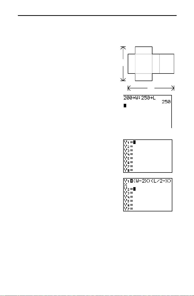
Defining a Function: Box with Lid
v
Take a 200×250 mm. sheet of paper and cut X-by-X squares from two corners and
X-by-125 mm. rectangles from the other two corners. Now fold the paper into a
box with lid. What X would give the maximum volume V of a box made in this
way? Use tables and graphs to determine the solution.
Begin by defining a function that describes the
olume of the box.
From the diagram: 2X + A = W
2X + 2B = L
V = A B X
Substituting: V = (W – 2X) (L à 2 – X) X
1. Press z †
to
Float
2. Press y
Í
to change the
MODE
back
.
ä
ã
Quit
‘
to return to the Home
screen and clear it.
ä
ã
3. Press
ƒ
¿ ƒ
200
Í
L
W y
to store the width and length of
:
¿
250
the paper.
4. You define functions for tables and graphing on
the
edit screen. Press o to access this
Y=
screen.
5. Enter the function for volume as
ƒ
¤ „ Í
„
. (
X
pressing
The
sign is highlighted to show that
=
„ ¤ £ ƒ
¹ 2
W
to define function
lets you enter X quickly, without
ƒ
.)
1
Y
L ¥ 2 ¹
Y
£
. Press
„
1
in terms of
1
is
Y
selected.
X
W
XABXB
L
6 Getting Started
Page 17
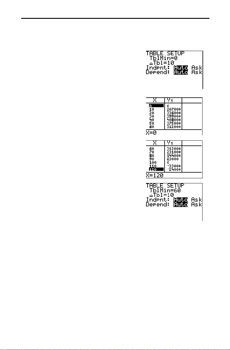
Defining a Table of Values
The table feature of the TI.82 provides numeric information about a function. Use
a table of values from the previously defined function to estimate an answer to
the problem.
ä
ã
TblSet
1. Press y
TABLE SETUP
2. Press
Í
3. Press 10
@
Tbl=10
. Leave
Í
(above
menu.
to accept
to define the table increment
Indpnt: Auto
so the table will be generated automatically.
ä
ã
4. Press y
TABLE
table.
Note that the maximum value displayed is at
. The maximum occurs between 30 and 50.
X=40
5. Press and hold † to scroll the table until the
sign change appears. Note that the maximum
length of
sign of
6. Press y
for this problem occurs where the
X
1
(volume) becomes negative.
Y
ä
ã
TblSet
. Note that
to reflect the first line of the table you last
displayed.
TblMin=0
(above
p
and
s
TblMin
) to display the
.
Depend: Auto
) to display the
has changed
Getting Started 7
Page 18
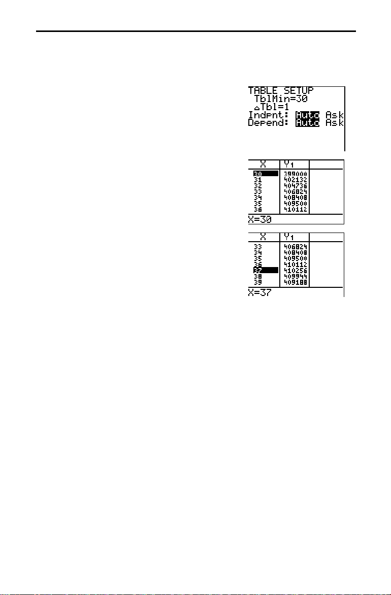
Zooming In on the Table
You can adjust the way a table is displayed to get more detailed information
about any defined function. By varying the value of @Tbl, you can “zoom in” on
the table.
1. Adjust the table setup to get a more accurate
estimate of the maximum size of the cutout.
Press
set
2. Press y
Í
.
ã
TABLE
to set
ä
.
30
@
Tbl
TblMin
. Press 1
3. Use † and } to scroll the table. Note that the
maximum value displayed is
occurs at
. The maximum occurs between
X=37
410256
36 and 38.
Í
, which
to
8 Getting Started
Page 19
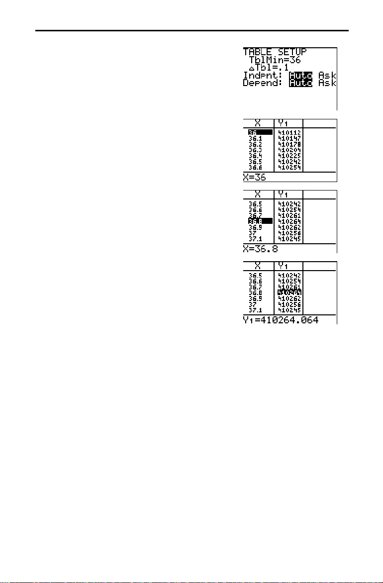
4. Press y
Press
.1
5. Press y
TblSet
Í
ã
TABLE
. Press
to set
ä
and use † and } to scroll the
Í
36
@
Tbl
to set
.
ä
ã
table.
6. Press † and } to move the cursor. The
maximum value of
1
at
36.8
is
410264
Y
TblMin
.
.
7. Press ~ to display the value of
precision,
410264.064
. This would be the
1
at
Y
maximum volume of the box if you could cut
your piece of paper at 1 mm. increments.
36.8
in full
Getting Started 9
Page 20
Changing the Viewing WINDOW
The viewing WINDOW defines the portion of the coordinate plane that appears in
the display. The values of the WINDOW variables determine the size of the
viewing WINDOW. You can view and change these values.
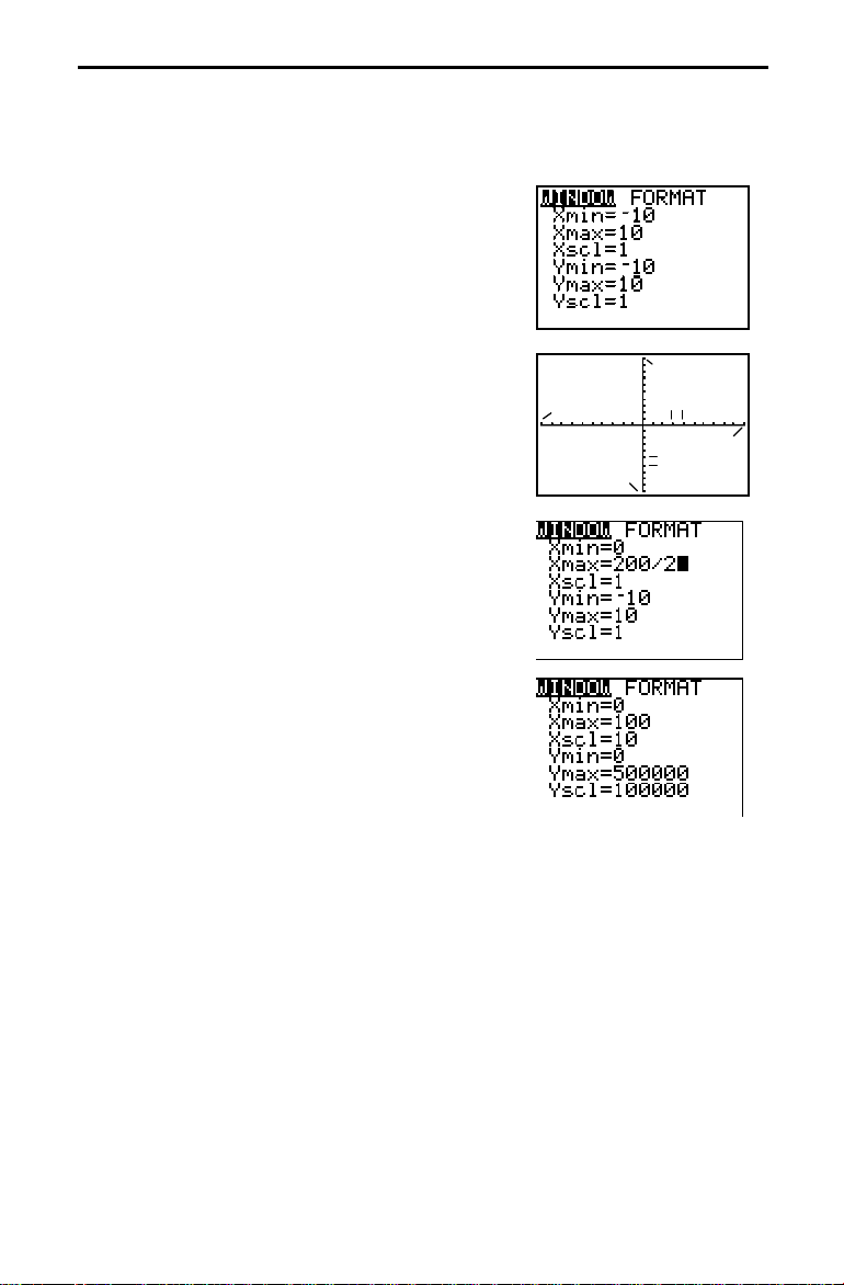
1. Press
p
to display the
WINDOW
variables
edit screen. You can view and edit the values of
the
WINDOW
The standard
viewing
and
Ymax
and
Xscl
marks on the
variables here.
WINDOW
WINDOW
variables define the
as shown.
Xmin, Xmax, Ymin
define the boundaries of the display.
define the distance between tick
Yscl
and Y axis.
X
2. Press † to move the cursor onto the line to
define
Xmin
. Press 0
Í
.
3. You can enter expressions to define values in
the
WINDOW
4. Press
is stored in
100
as 10.
Xscl
5. Press 0
define the
editor. Press
Í
. The expression is evaluated, and
. Press 10
Xmax
Í
Y
WINDOW
500000
Í
variables.
200
100000
¥ 2.
Í
to set
Í
to
,
Ymax
Xmin
Xscl
Xmax
Yscl
Ymin
10 Getting Started
Page 21
Displaying and Tracing the Graph
Now that you have defined the function to be graphed and the WINDOW in which
to graph it, you can display and explore the graph. You can trace along a function
with TRACE.
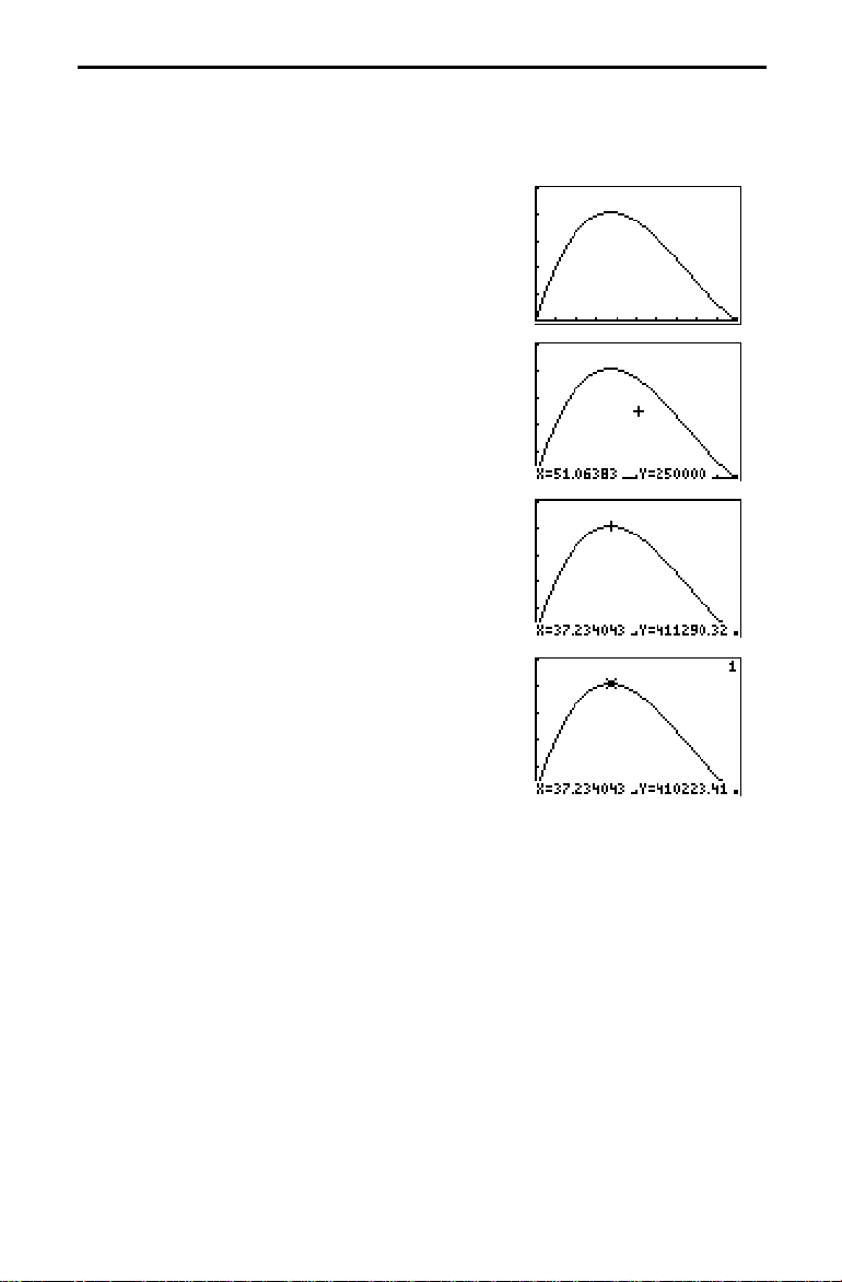
1. Press
s
the viewing
The graph of
to graph the selected function in
WINDOW
Y1=(W–2X)(Là2–X)X
.
is shown in
the display.
2. Press ~ once to display the free-moving graph
cursor just to the right of the center of the
screen. The bottom line of the display shows the
and Y coordinate values for the position of the
X
graph cursor.
3. Use the cursor-keys (|, ~, }, and †) to
position the free-moving cursor at the apparent
maximum of the function.
As you move the cursor,
and Y coordinate
X
values are updated continually with the cursor
position.
4. Press
r
. The
1
function near the middle of the screen. 1 in
Y
cursor appears on the
TRACE
the upper right corner of the display shows that
the cursor is on
trace along
1
. As you press | and ~, you
Y
1
, one X dot at a time, evaluating
Y
at each X.
Press | and ~ until you are on the maximum
value. This is the maximum of
Y1(X)
for the
X
pixels. (There may be a maximum “in between”
pixels.)
1
Y
Y
Getting Started 11
Page 22
Zooming on the Graph
You can magnify the viewing WINDOW around a specific location using the
ZOOM instructions to help identify maximums, minimums, roots, and
intersections of functions.
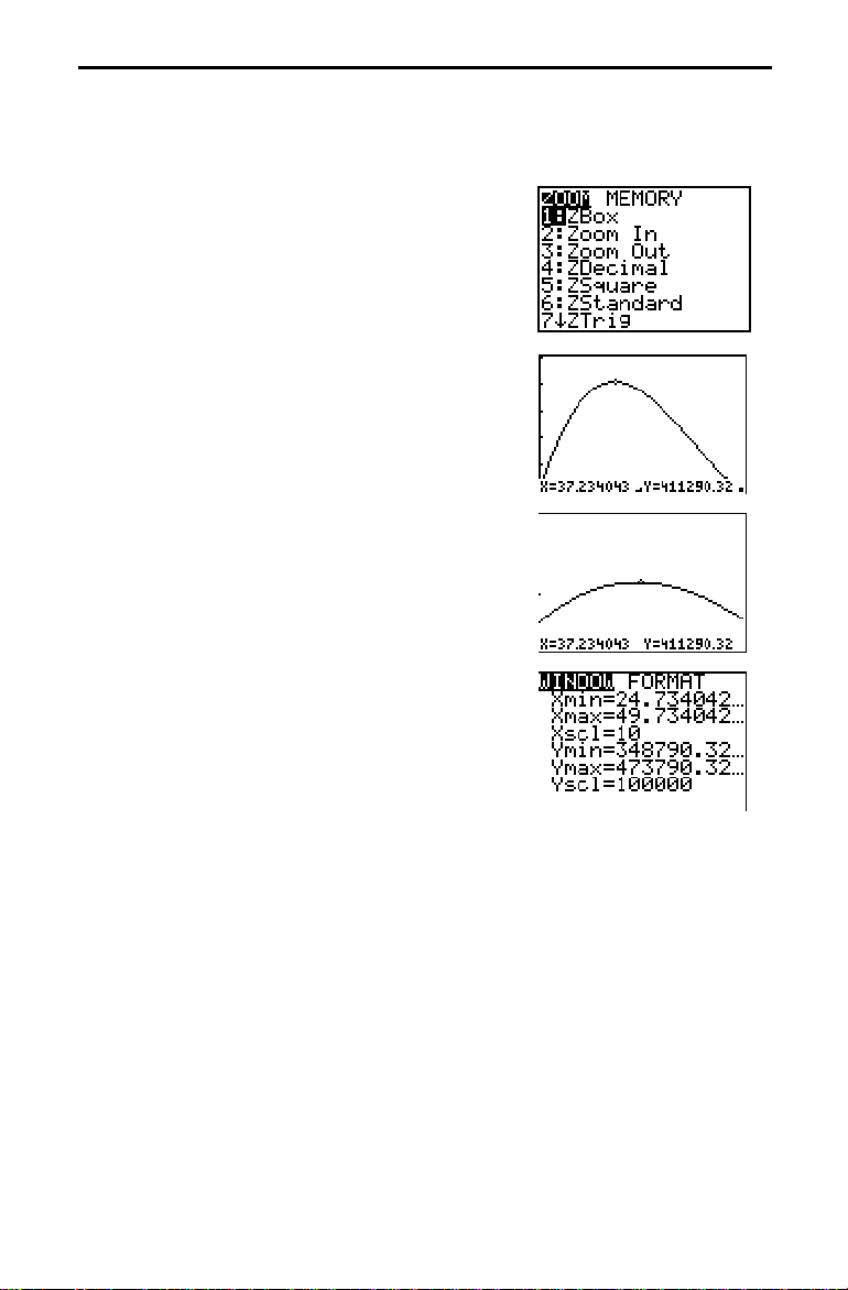
1. Press
q
to display the
ZOOM
menu.
This menu is typical of TI.82 menus. To select
an item, you may either press the number to the
left of the item, or you may press † until the
item number is highlighted and then press
Í
.
2. To zoom in, press 2. The graph is displayed
again. The cursor has changed to indicate that
you are using a
ZOOM
instruction.
3. Use |, }, ~, and † to position the cursor near
the maximum value on the function and press
Í
.
The new viewing
WINDOW
been adjusted in both the
factors of 4, the values for
4. Press
p
to display the new
is displayed. It has
and Y directions by
X
factors.
ZOOM
WINDOW
settings.
12 Getting Started
Page 23
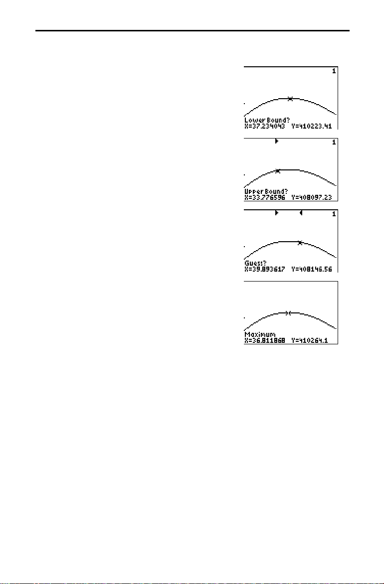
Finding the Calculated Maximum
You can use a CALC operation to calculate a local maximum of a function.
ä
ã
CALC
1. Press y
menu. Press 4 to select
The graph is displayed again, with a prompt for
Lower Bound?
2. Use | to trace along the curve to a point to the
left of the maximum and then press
A triangle at the top of the screen indicates the
selected bound. A new prompt is displayed for
Upper Bound?
3. Use ~ to trace along the curve to a point to the
right of the maximum and then press
A triangle at the top of the screen indicates the
selected bound. A new prompt is displayed for
Guess?
4. Use | to trace to a point near the maximum and
Í
press
bottom of the display.
Note how the values for the calculated
maximum compared with the maximums found
with the free-moving cursor,
table.
to display the
maximum
CALCULATE
.
Í
Í
. The answer is displayed at the
, and the
TRACE
.
.
Getting Started 13
Page 24

Other Features
Getting Started introduced you to basic calculator operation and the table and
function graphing features of the TI.82. The remainder of this guidebook
describes these features in more detail and also covers other capabilities of the
TI.82.
Graphing
You can store, graph, and analyze up to ten functions (Chapter 3), up to six
parametric functions (Chapter 4), and up to six polar functions (Chapter 5).
You can use
Sequences
You can generate sequences and graph them over time or as web plots.
(Chapter 6)
Tables
You can create function evaluation tables to analyze multiple functions
simultaneously. (Chapter 7)
Matrices
You can enter and save up to five matrices and perform standard matrix
operations on them. (Chapter 10)
Lists
You can enter and save up to six lists for use in statistical analysis. You also
can use lists to evaluate expressions at multiple values simultaneously and
to graph a family of curves. (Chapter 11)
operations to annotate graphs (Chapter 8).
DRAW
Statistics
You can perform one-variable and two-variable list-based statistical
analysis, including median-median line and regression analysis, and plot the
data as histograms, points,
lines, or box-and-whisker plots. You can
x-y
define and save three statistical plot definitions. (Chapters 12).
Programming
You can enter and save programs that include extensive control and
input/output instructions. (Chapter 13)
Split Screen
You can show simultaneously the graph screen and a related editor, such as
the
screen, table, list editor, or Home screen. (Chapter 9)
Y=
14 Getting Started
Page 25

Chapter 1: Operating the TI-82
This chapter describes the TI.82 and provides general information about its
operation.
Chapter Contents
Turning the TI.82 On and Off
Setting the Display Contrast
The Display
................................
Entering Expressions and Instructions
TI.82 Edit Keys
Setting Modes
TI.82 Modes
Variable Names
..............................
...............................
................................
..............................
Storing and Recalling Variable Values
..................................
Last Entry
Last Answer
TI.82 Menus
VARS
EOS
Error Conditions
.................................
................................
and
Y.VARS
é
Equation Operating System
(
Menus
.............................
......................
.....................
.............
..............
.......................
................
)
1-2
1-3
1
1
1
1
-
1
10
-
1
12
-
1
13
1-14
1-16
-
1
17
1-19
1-20
-
1
22
-
4
-
6
-
8
-
9
Operating the TI.82 1-1
Page 26

Turning the TI-82 On and Off
To turn the TI.82 on, press the É key. To turn it off, press and release y and
then press M. After about five minutes without any activity, APDé (Automatic
Power Down™) turns the TI.82 off automatically.
Turning the Calculator On
Press É to turn the TI.82 on.
ä
¦
If you pressed y
the Home screen as it was when you last used it, and errors are cleared.
¦
If APD turned the calculator off, the TI.82, including the display, cursor,
and any error conditions, will be exactly as you left it.
Turning the Calculator Off
Press and release y and then press
¦
Any error condition is cleared.
¦
All settings and memory contents are retained by Constant Memoryé.
APD™ (Automatic Power Down™)
To prolong the life of the batteries, APD turns the TI.82 off automatically
after several minutes without any activity. When you press É, the TI.82
will be exactly as you left it.
¦
The display, cursor, and any error conditions are exactly as you left
them.
¦
All settings and memory contents are retained by Constant Memory.
ã
OFF
to turn the calculator off, the display shows
ä
ã
OFF
to turn the TI.82 off.
Batteries
The TI.82 uses four AAA alkaline batteries and has a user-replaceable backup lithium battery. To replace batteries without losing any information
stored in memory, follow the directions on page B.2.
1-2 Operating the TI.82
Page 27

Setting the Display Contrast
The brightness and contrast of the display depends on room lighting, battery
freshness, viewing angle, and adjustment of the display contrast. The contrast
setting is retained in memory when the TI.82 is turned off.
Adjusting the Display Contrast
You can adjust the display contrast to suit your viewing angle and lighting
conditions at any time. As you change the contrast setting, the display
contrast changes, and a number in the upper right corner indicates the
current contrast setting between 0 (lightest) and 9 (darkest).
Note that there are 32 different contrast levels, so each number 0 through 9
represents more than one setting.
To adjust the contrast:
1. Press and release the y key.
2. Use one of two keys:
¦
To increase the contrast, press and hold }.
¦
To decrease the contrast, press and hold †.
Note: If you adjust the contrast setting to zero, the display may become
completely blank. If this happens, press and release y and then press and
hold } until the display reappears.
When to Replace Batteries
When the batteries are low, the display begins to dim (especially during
calculations), and you must adjust the contrast to a higher setting. If you
find it necessary to set the contrast to a setting of 8 or 9, you should replace
the four AAA batteries soon.
Note: The display contrast may appear very dark after you change
batteries. Press and release y and then press and hold † to lighten the
display.
Operating the TI.82 1-3
Page 28
The Display
The TI.82 displays both text and graphics. Graphics are described in Chapter 3.
The TI.82 also can display a split screen, showing graphics and text
simultaneously (Chapter 9).
Home Screen
The Home screen is the primary screen of the TI.82, where you enter
instructions to be executed and expressions to be evaluated and see the
answers.
Displaying Entries and Answers
When text is displayed, the TI.82 screen can have up to eight lines of up to
16 characters per line. If all lines of the display are filled, text “scrolls” off
the top of the display. If an expression on the Home screen, the
(Chapter 3), or the program editor (Chapter 13) is longer than one line, it
wraps to the beginning of the next line. On numeric editors such as the
WINDOW
screen (Chapter 3), an expression scrolls to the left and right.
When an entry is executed on the Home screen, the answer is displayed on
the right side of the next line.
Entry
Answer
Y=
editor
The
settings control the way expressions are interpreted and
MODE
answers are displayed (page 1.10).
If an answer, such as a list or matrix, is too long to display in its entirety,
ellipsis marks (...) are shown at the left or right. Use ~ and | to scroll the
answer and view all of it.
Returning to the Home Screen
Entry
Answer
To return to the Home screen from any other screen, press y
1-4 Operating the TI.82
ã
QUIT
ä
.
Page 29

Display Cursors
In most cases, the appearance of the cursor indicates what will happen
when you press the next key.
Cursor Appearance Meaning
Entry Solid blinking
rectangle
(insert) Blinking underline The next keystroke is inserted in front
INS
The next keystroke is entered at the
cursor; it types over any character.
of the cursor location.
2nd
ALPHA
Blinking # (arrow) The next keystroke is a
Blinking
A
The next keystroke is an alphabetic
character.
“full” Checkerboard
rectangle
You have entered the maximum
characters in a name, or memory is
full.
operation.
2nd
If you press
to an underlined
If you press y or
(such as the
ƒ
or y during an insertion, the underline cursor changes
or # cursor.
A
ƒ
on a screen on which there is no edit cursor
screen or a graph), # or A appears in the upper right
MODE
corner.
Graphs and the screens for viewing and editing tables, matrices, and lists
have different cursors, which are described in the appropriate chapter.
Busy Indicator
When the TI.82 is calculating or graphing, a moving vertical bar shows in
the upper right of the display as a busy indicator. (When you pause a graph
or a program, the busy indicator is a dotted bar.)
Operating the TI.82 1-5
Page 30
Entering Expressions and Instructions
On the TI.82, you can enter expressions, which return a value, in most places
where a value is required. You enter instructions, which initiate an action, on the
Home screen or in the program editor (Chapter 13).
Expressions
An expression is a complete sequence of numbers, variables, functions, and
their arguments that evaluate to a single answer. On the TI.82, you enter an
Í
4 5
p
. You
R
expression in the same order that it normally is written. For example,
is an expression.
Expressions can be used on the Home screen to calculate an answer. In
most places where a value is required, expressions may be used to enter a
value.
Entering an Expression
To create an expression, enter numbers, variables, and functions from the
keyboard and menus. An expression is completed when you press
regardless of the cursor location. The entire expression is evaluated
according to EOS rules (page 1.20), and the answer displayed.
Most TI.82 functions and operations are symbols with several characters in
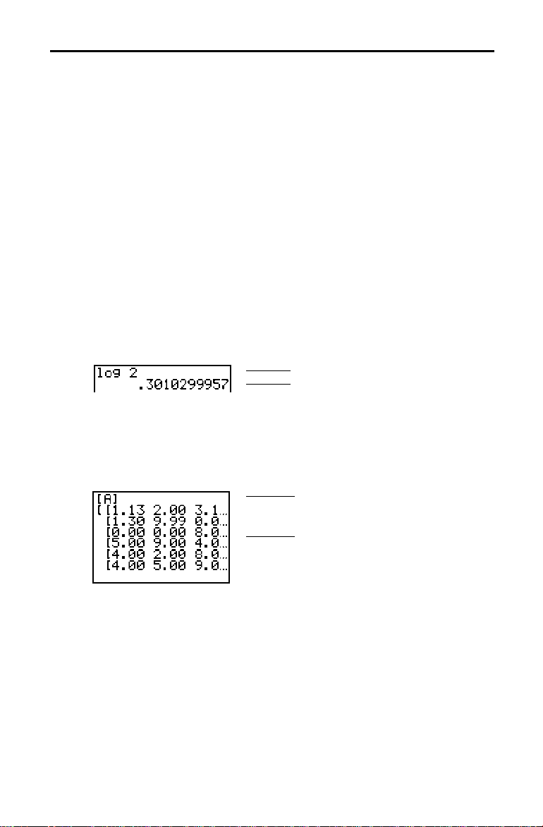
them. You must enter the symbol from the keyboard or menu, not spell it
out. For example, to calculate the log of 45, you must press «
cannot type in the letters
entry as implied multiplication of the variables
L O G
. (If you type
, the TI.82 interprets the
LOG
, and G.)
L, O
2
,
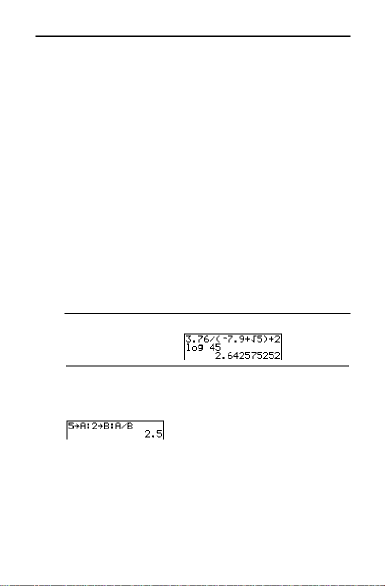
Calculate 3.76 ÷ (-7.9 + ‡5) + 2 log 45.
Multiple Entries on a Line
1-6 Operating the TI.82
¥ £ Ì
3.76
¤ Ã 2 «
5
Í
To enter more than one expression or instruction on a line, separate them
with a colon (
à y
7.9
45
). They are all stored together in
:
‡
ä
ã
Last Entry
(page 1.14).
Page 31

Entering a Number in Scientific Notation
1. Type the part of the number that precedes the exponent. This value can
be an expression.
ã
ä
E
2. Press y
EE
.
appears in the display.
3. If the exponent is negative, press Ì and then type the exponent, which
can be one or two digits.
Entering a number in scientific notation does not cause the answers to be
displayed in scientific or engineering notation. The display format is
determined by the
Functions
A function returns a value. For example, ÷, -, +, ‡, and
settings (page 1.10) and the size of the number.
MODE
log
functions in the previous example. In general, the names of functions on
the display begin with a lowercase letter. Some functions take more than
one argument, which is indicated by a
example,
Instructions
requires arguments,
min(
An instruction initiates an action. For example,
at the end of the name. For
(
min(5,8)
.
ClrDraw
is an instruction
that clears any drawn elements from a graph. Instructions cannot be used
in expressions. In general, the names of instructions begin with a capital
letter. Some instructions require more than one argument, which is
indicated by a
arguments,
at the end of the name. For example,
(
Circle(0,0,5)
.
Circle(
were the
requires three
Interrupting a Calculation
While the busy indicator is displayed, indicating that a calculation or a
graph is in progress, you can press É to stop the calculation. (There may
be a delay.) Except in graphing, the
¦
To go to where the interruption occurred, select
¦
To return to the Home screen, select
ERR:BREAK
screen is shown.
.
Quit
Goto
Operating the TI.82 1-7
.
Page 32

TI-82 Edit Keys
~
|
or
}
†
or
y |
y ~
Í
‘ ¦
{
ã
y
INS
y
ƒ
ã
y
A-LOCK
„
Moves the cursor within an expression. These keys repeat.
Moves the cursor between lines. These keys repeat.
¦
¦
Moves the cursor to beginning of expression.
Moves the cursor to end of expression.
Evaluates an expression or executes an instruction.
¦
¦
Deletes character at cursor. This key repeats.
ä
Inserts characters at underline cursor. To end insertion, press
ã
Next keystroke performs a
left above a key). The cursor changes to an #. To cancel
y
Next keystroke is an
right above the key). The cursor changes to an A. To cancel
press
ä
Sets
character. The cursor changes to an A. To cancel
press
keyboard in
Allows you to enter an
Pol
On top line of an expression on the Home screen, } moves the
cursor to beginning of expression.
On bottom line of an expression on the Home screen, † moves
the cursor to end of expression.
On a line with text on the Home screen, clears (blanks) the
current line.
On a blank line on the Home screen, clears everything on the
Home screen.
In an editor, clears (blanks) expression or value where cursor is
located; it does not store a zero.
ä
INS
or a cursor-key.
operation (the blue operation to the
2nd
2nd
, press
.
character (the gray character to the
ALPHA
ƒ
or a cursor-key.
ALPHA-LOCK
ƒ
MODE
; each subsequent keystroke is an
ALPHA
ALPHA-LOCK
. Note that prompts for names automatically set the
ALPHA-LOCK
without pressing
.
in
X
Func
ƒ
MODE
first.
, a T in
Par
MODE
, or a q in
y
ALPHA
,
,
1-8 Operating the TI.82
Page 33

Setting Modes
Modes control how numbers and graphs are displayed and interpreted. MODE
settings are retained by Constant Memoryé when the TI.82 is turned off. All
numbers, including elements of matrices and lists, are displayed according to the
current MODE settings.
Checking MODE Settings
Press z to display the
highlighted. The specific
pages.
settings. The current settings are
MODE
settings are described on the following
MODE
Normal Sci Eng
Float 0123456789
Radian Degree
Func Par Pol Seq
Connected Dot
Sequential Simul
FullScreen Split
Changing MODE Settings
Numeric display format
Number of decimal places
Unit of angle measure
Type of graphing
Whether to connect graph points
Whether to plot simultaneously
Full or split screen
1. Use † or } to move the cursor to the line of the setting that you want
to change. The setting that the cursor is on blinks.
2. Use ~ or | to move the cursor to the setting that you want.
3. Press
Leaving the MODE Screen
To leave the
¦
¦
Setting a MODE from a Program
You can set a
an instruction; for example,
name from the interactive
Í
.
screen:
MODE
Press the appropriate keys to go to another screen.
ä
ã
Press y
QUIT
MODE
‘
or
to return to the Home screen.
from a program by entering the name of the
or
Func
selection screen in the program editor
MODE
. From a blank line, select the
Float
(Chapter 13); the name is copied to the cursor location. The format for
fixed decimal setting is
Fix
n
.
MODE
as
Operating the TI.82 1-9
Page 34

TI-82 Modes
The TI.82 has seven MODE settings. Three are related to how numeric entries are
interpreted or displayed and four are related to how graphs appear in the display.
Modes are set on the MODE screen (page 1.9).
Normal, Sci, Eng
Notation formats affect only how an answer is displayed on the Home
screen. Numeric answers can display with up to 10 digits and a two-digit
exponent. You can enter a number in any format.
display format is the way in which we usually express numbers,
Normal
with digits to the left and right of the decimal, as in
(scientific) notation expresses numbers in two parts. The significant
Sci
12346.67
digits display with one digit to the left of the decimal. The appropriate
power of 10 displays to the right of
(engineering) notation is similar to scientific notation. However, the
Eng
E
, as in
1.234667E4
number may have one, two, or three digits before the decimal, and the
power-of-10 exponent is a multiple of three, as in
12.34667E3
Note: If you select normal display format, but the answer cannot display in
10 digits or the absolute value is less than .001, the TI.82 changes to
scientific notation for that answer only.
Float, Fix
Decimal settings affect only how an answer is displayed on the Home
screen. They apply to all three notation display formats. You can enter a
number in any format.
(floating) decimal setting displays up to 10 digits, plus the sign and
Float
decimal.
The fixed decimal setting displays the selected number of digits (
the right of the decimal. Place the cursor on the number of decimal digits
you want and press
Í
.
.
.
.
to 9) to
0
1-10 Operating the TI.82
Page 35

Radian, Degree
Angle settings control how the TI.82 interprets angle values in trig
functions and polar/rectangular conversions.
interprets the values as radians. Answers display in radians.
Radian
interprets the values as degrees. Answers display in degrees.
Degree
Func, Par, Pol, Seq
(function) graphing plots functions where Y is a function of
Func
(Chapter 3).
(parametric) graphing plots relations where X and Y are functions of
Par
(Chapter 4).
(polar) graphing plots functions where R is a function of q (Chapter 5).
Pol
(sequence) graphing plots sequences (Chapter 6).
Seq
Connected, Dot
Connected
draws a line between the points calculated for the selected
functions.
plots only the calculated points of the selected functions.
Dot
Sequential, Simul
Sequential
graphing evaluates and plots one function completely before the
next function is evaluated and plotted.
(simultaneous) graphing evaluates and plots all selected functions
Simul
for a single value of
of
.
X
and then evaluates and plots them for the next value
X
X
T
FullScreen, Split
FullScreen
Split
uses the entire screen to display a graph or edit screen.
screen displays the current graph on the upper portion of the screen
and the Home screen or an editor on the lower portion (Chapter 9).
Operating the TI.82 1-11
Page 36

Variable Names
On the TI.82 you can enter and use several types of data, including real numbers,
matrices, lists, functions, stat plots, graph databases, and graph pictures.
Variables and Defined Items
The TI.82 uses preassigned names for variables and other items saved in
memory.
Variable type Names
2
,
L
2
, . . . ,
1T
3
,
r
n
3
,
L
, . . . ,
4
,
,
r
, . . . ,
4
Y
r
q
5
6
,
,
L
L
9
0
,
Y
6T
X6T/Y
5
6
,
r
, . . . ,
GDB6
Pic6
, and others
Real numbers
Matrices
Lists
Functions
Parametric equations
Polar functions
Sequence functions
Stat plots
Graph databases
Graph pictures
System variables
, . . . , Z,
A, B
ãAä, ãBä, ãCä, ãDä, ãEä
1
,
L
L
1
,
Y
Y
X1T/Y
1
2
,
r
r
,
U
n
V
Plot1, Plot2, Plot3
GDB1, GDB2
Pic1, Pic2
Xmin, Xmax
Programs have user-defined names also and share memory with variables.
Programs are entered and edited from the program editor (Chapter 13).
You can store to matrices (Chapter 10), lists (Chapter 11), system variables
such as
(Chapter 3) or
Xmax
(Chapter 7), and all functions
TblMin
(Chapters 3, 4, 5, and 6) from the Home screen or from a program. You can
store to matrices (Chapter 10), lists (Chapter 12), and functions (Chapter 3)
from editors. You can store to a matrix element (Chapter 10) or a list
element (Chapter 11). Graph databases and pictures are stored and recalled
using instructions from the
menu (Chapter 8).
DRAW
1-12 Operating the TI.82
Page 37

Storing and Recalling Variable Values
Values are stored to and recalled from memory using variable names. When an
expression containing the name of a variable is evaluated, the value of the
variable at that time is used.
Storing Values in a Variable
You can store a value to a variable from the Home screen or a program
using the ¿ key. Begin on a blank line.
1. Enter the value that you want to store (which can be an expression).
2. Press ¿. The symbol
3. Press
ƒ
, then the letter of the variable to which you want to store
the value.
4. Press
Í
. If you entered an expression, it is evaluated. The value is
stored in the variable.
Displaying a Variable Value
To display the value of a variable, enter the name on a blank line on the
Home screen, and press
RCL (Recall)
You can copy variable contents to the current cursor location. Press
ä
ã
RCL
, and then enter the name of the variable in one of the following ways:
¦
¦
¦
¦
¦
ƒ
Press
and then the letter of the variable.
Press y and the name of the list.
Press
Press y
Press
and select the name of the matrix.
ã
Y.VARS
and select the name of the program (in the program editor
only).
You can edit the characters copied to the expression without affecting the
value in memory.
Note: When an error (such as a variable with no assigned value) occurs on
the
name. To leave
line, the name is cleared automatically for you to enter the correct
RCL
without recalling a value, press
RCL
!
is copied to the cursor location.
Í
.
ä
and select the type and name of the function.
‘
.
y
Operating the TI.82 1-13
Page 38

Last Entry
Last Entry
7
ã
ENTRY
ƒ
ã
ENTRY
Í
on the Home screen to evaluate an expression or execute
Last Entry
ã
ENTRY
, it replaces what you have typed.
ä
). They are all stored together in
:
R y ã:ä y
ä
and edit it from the Home screen or any editor.
ä
. On the Home screen or a numeric editor, the current
Last Entry
Í
is copied to the line. The cursor is
Last Entry
is pressed, you can recall the previous entry
Last Entry
2
, use trial and error to find the radius of a circle
ãpä
R
ƒ
¡
(page 1.14).
Last Entry
When you press
an instruction, the expression or instruction is stored in a storage area called
Last Entry, which you can recall. When you turn the TI.82 off, Last Entry is
retained in memory.
Using Last Entry
You can recall
Press y
line is cleared and the
positioned at the end of the entry. In the program editor, the
inserted at the cursor location. Because the TI.82 updates the
storage area only when
even if you have begun entering the next expression. However, when you
recall
Ã
5
Í
y
Multiple Entries on a Line
To enter more than one expression or instruction on a line, separate them
with a colon (
If the previous entry contained more than one expression or instruction,
separated with a colon (page 1.7), they all are recalled. You can recall all
entries on a line, edit any of them, and then execute all of them.
Using the equation A=pr
that covers 200 square centimeters. Use 8 as your first guess.
¿
8
Í
y
is
y
7
y |
Í
Continue until the answer is as accurate as you want.
1-14 Operating the TI.82
.95
ä
ã
INS
Page 39

Reexecuting the Previous Entry
To execute
entry does not display again.
¿
0
Í
ƒ
y
Í
Í
Accessing a Previous Entry
The TI.82 retains as many of the previous entries as is possible (up to a
total of 128 bytes) in the
entries by continuing to press y
128 bytes, it is retained for
Last Entry
¿
1
Í
¿
2
Í
¿
3
Í
y
Each time you press y
press y
displayed.
ƒ
à 1 ¿
N
ƒ
ã:ä
storage area.)
ƒ
ƒ
ƒ
ã
ENTRY
Last Entry
N
ƒ
Í
¡
N
A
B
C
ä
ã
ä
ENTRY
after displaying the oldest item, the newest item is
press
Last Entry
ã
Í
on a blank line on the Home screen; the
N
storage area. You can access those
ã
ä
ENTRY
. (If a single entry is more than
Last Entry
ENTRY
, but it cannot be placed in the
ä
, the current line is overwritten. If you
y
ã
ENTRY
ä
Operating the TI.82 1-15
Page 40

Last Answer
When an expression is evaluated successfully from the Home screen or from a
program, the TI.82 stores the answer to a variable, Ans (Last Answer). Ans may
be a real number, a list, or a matrix. When you turn the TI.82 off, the value in Ans
is retained in memory.
Using Ans in an Expression
You can use the variable
ã
ä
Press y
When the expression is evaluated, the TI.82 uses the value of
calculation.
Calculate the area of a garden plot 1.7 meters by 4.2 meters. Then calculate
the yield per square meter if the plot produces a total of 147 tomatoes.
1.7
Í
147
Í
Continuing an Expression
You can use the value in
without entering the value again or pressing y
the Home screen, enter the function. The TI.82 “types” the variable name
Ans
¥
5
Í
¯
9.9
Í
ANS
and the variable name
¯
4.2
ä
ã
¥ y
followed by the function.
ANS
2
to represent the last answer in most places.
Ans
is copied to the cursor location.
Ans
Ans
as the first entry in the next expression
Ans
ã
ä
ANS
. On the blank line on
in the
Storing Answers
To store an answer, store
expression.
Calculate the area of a circle of radius 5 meters. Then calculate the volume
of a cylinder of radius 5 meters and height 3.3 meters and store in the
variable
y
Í
¯
Í
¿ ƒ
Í
1-16 Operating the TI.82
3.3
ãpä
.
V
¡
5
V
to a variable before you evaluate another
Ans
Page 41

TI-82 Menus
To leave the keyboard uncluttered, the TI.82 uses full-screen menus to access
many operations. The use of specific menus is described in the appropriate
chapters.
Moving from One Menu to Another
A menu key may access more than one menu. The names of the menus
appear on the top line. The current menu is highlighted and the items in
that menu are displayed.
Use ~ or | to move the cursor to a different menu.
Selecting an Item from a Menu
The number of the current item is highlighted. If there are more than seven
items on the menu, a
Menu items that end in
There are two methods of selecting from a menu.
¦
Press the number of the item you want to select.
¦
Use † and } to move the cursor to the item you want to select and
then press
Leaving a Menu without Making a Selection
After you make a selection from a menu, you usually are returned to the
screen where you were.
To leave a menu without making a selection, do any of the following:
¦
Press y
¦
¦
¦
‘
Press
Display a different menu by pressing the appropriate key, such as
Select another screen by pressing the appropriate key, such as
$
appears on the last line in place of the : (colon).
(ellipsis marks) access another menu.
...
Í
.
ä
ã
QUIT
to return to the Home screen.
to return to the screen where you were.
p
.
.
Operating the TI.82 1-17
Page 42

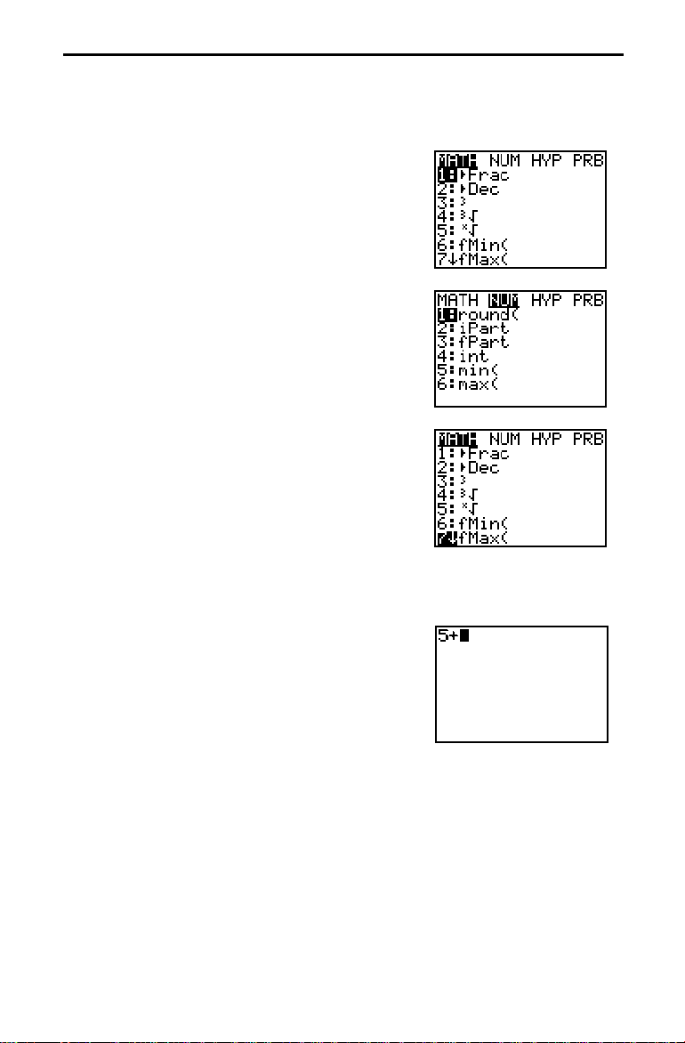
Calculate 6
1. Press 6. Press
2. To select
3. Press 27 and then press
3
‡
27.
to display the
3
‡
, you may either press 4 or press † † †
Í
to evaluate the expression.
MATH
menu.
Í
.
1-18 Operating the TI.82
Page 43
VARS and Y-VARS Menus
Occasionally you may want to access the names of functions and system
variables to use in an expression or to store to them directly. Use the VARS or
Y.VARS menus to access the names of variables such as Xmin and functions
1
such Y
VARS Menu
Y-VARS Menu
.
The
and
databases and graph pictures such as
such as
Press
menu accesses the names of
VARS
, the user-defined
Tstep
v
,
RegEQ
to display the
1
and
, and table variables such as
Q
WINDOW
variables such as
ZOOM
VARS
GDB1
menu. Some of the items access more than
variables such as
ZXmin
and
, statistics variables
Pic2
TblMin
, graph
.
one menu of variable names.
VARS
1: Window
2: Zoom
3: GDB
4: Picture
5: Statistics
6: Table
The
…
…
…
…
Y-VARS
q
,
X/Y, T/
ZX/ZY, ZT/Z
GDB
Pic
Table
U/V
n
variables
n
variables
BOX, PTS
variables
variables
q
, ZU variables
variables
…
Names of
Names of
Names of
Names of
…
X/Y
Names of
, G, EQ,
menu accesses the names of functions and the instructions to
select or deselect functions from a program or the Home screen.
Press y
Y-VARS
1: Function
2: Parametric
3: Polar
4: Sequence
5: On/Off
ã
…
…
Y-VARS
…
…
…
to display the
ä
Displays names of
Displays names of
Displays names of
Displays names of
Y-VARS
Y
X
r
U
menu.
n
functions
n
n
T
,
Y
n
functions
n
n
,
functions
V
T
Lets you select/deselect functions
functions
Xmin
Accessing a Name from a VARS or Y-VARS Menu
1. Press
or y
2. Select the type of name you want;
In
¦
In
¦
, use ~ or | to move to the menu you want, if necessary.
VARS
Y-VARS
Y-VARS
ã
. The
ä
VARS
Picture...
, a single menu is displayed.
or
Y-VARS
or
Polar...
3. Select the name you want from the menu. It is copied to the cursor
location.
Operating the TI.82 1-19
menu is displayed.
, for example.
Page 44

EOS™ (Equation Operating System)
v
The Equation Operating System (EOSé) defines the order in which functions in
expressions are entered and evaluated on the TI.82. EOS lets you enter numbers
and functions in a simple, straightforward sequence.
Order of Evaluation
A function returns a value. EOS evaluates the functions in an expression in
the following order:
Functions that are entered after the argument, such as 2, -1, !, ¡, r,
1
T
, and conversions.
x
Powers and roots, such as
2
Implied multiplication where the second argument is a number,
3
2^5
ariable name, list, or matrix or begins with an open parenthesis,
such as 4A,
Single-argument functions that precede the argument, such as
4
negation, ‡,
Implied multiplication where the second argument is a
5
3ãB
sin
ä
,
(A+B)4
, or
log
, or
.
multiargument function or a single-argument function that
precedes the argument, such as
Permutations (
6
Multiplication and division.
7
Addition and subtraction.
8
Relational functions, such as > or .
9
Logic operator
10
Logic operators or and
11
) and combinations (
nPr
.
and
.
xor
‡
or
32
5
.
4(A+B)
2nDeriv(A2,A,6)
.
nCr
or
Asin 2
.
).
Within a priority group, EOS evaluates functions from left to right.
However, two or more single-argument functions that precede the same
argument are evaluated from right to left. For example,
evaluated as
sin(fPart(ln 8))
.
sin fPart ln 8
is
Calculations within a pair of parentheses are evaluated first. Multiargument
functions, such as
nDeriv(A2,A,6)
, are evaluated as they are encountered.
1-20 Operating the TI.82
Page 45

Implied Multiplication
The TI.82 recognizes implied multiplication. For example, it understands
p
,
2
Parentheses
4 sin 46, 5(1+2)
, and
as implied multiplication.
(2…5)7
All calculations inside a pair of parentheses are completed first. For
example, in the expression
the parentheses,
, and then multiplies the answer, 3, by 4.
1+2
, EOS first evaluates the portion inside
4(1+2)
You can omit any right (close) parenthesis at the end of an expression. All
“open” parenthetical elements are closed automatically at the end of an
expression and preceding the
!
(store) or display conversion instructions.
Note: If the name of a list or matrix is followed by an open parenthesis, it
does not indicate implied multiplication. It is used to access specific
elements in the list (Chapter 11) or matrix (Chapter 10).
Negation
To enter a negative number, use the negation function. Press Ì and then
enter the number. On the TI.82, negation is in the fourth group in the EOS
hierarchy. Functions in the first group, such as squaring, are evaluated
before negation.
2
For example,
M
is a negative number (or 0);
X
square a negative number:
(M9)
2
.
2
M
M
is
9
. Use parentheses to
81
Note: Use the ¹ key for subtraction and the Ì key for negation. If you
press ¹ to enter a negative number, as in
indicate subtraction, as in
, it is interpreted as implied multiplication (
B
ƒ
Ì 7, it is an error. If you press
9
¯ ¹ 7, or if you press Ì to
9
A
ƒ
).
A…MB
Ì
Operating the TI.82 1-21
Page 46

Error Conditions
The TI.82 detects any errors at the time it evaluates an expression, executes an
instruction, plots a graph, or stores a value. Calculations stop and an error
message with a menu displays immediately. Error codes and conditions are
described in detail in Appendix B.
Diagnosing an Error
If the TI.82 detects an error, it displays the error screen.
The top line indicates the general type of error, such as
DOMAIN
. Additional information about each error message is in Appendix
SYNTAX
B.
¦
If you select
, the cursor is displayed at the location where the
Goto
error was detected.
Note: If a syntax error was detected in the contents of a
during program execution, this option returns the user to the
not the program.
ä
¦
If you select
or press y
Quit
ã
QUIT
or
‘
, you return to the Home
screen.
Correcting an Error
1. Note the type of the error.
2. Select
, if that option is available, and look at the expression for
Goto
syntax errors, especially at and in front of the cursor location.
3. If the error in the expression is not readily apparent, turn to Appendix B
and read the information about the error message.
4. Correct the expression.
or
function
Y=
Y=
editor,
1-22 Operating the TI.82
Page 47

Chapter 2: Math, Angle, and Test Operations
This chapter describes math, angle, and relational operations that are available
on the TI.82. The most commonly used functions are accessed from the
keyboard; others are accessed through full-screen menus.
Chapter Contents
Getting Started: Lottery Chances
Keyboard Math Operations
MATH MATH
MATH NUM
MATH HYP
MATH PRB
Operations
ANGLE
TEST TEST
TEST LOGIC
Operations
(Number) Operations
(Hyperbolic) Operations
(Probability) Operations
(Relational) Operations
(Boolean) Operations
.........................
.............................
...................
.......................
..................
.................
.................
.................
.................
2-2
2-3
2-5
2-9
2-11
2-12
2-13
2-15
2-16
Math, Angle, and Test Operations 2-1
Page 48

Getting Started: Lottery Chances
Getting Started is a fast-paced introduction. Read the chapter for details.
Suppose you want to enter a lottery where 6 numbers will be drawn out of 49. To
win, you must pick all 6 numbers (in any order). What is the probability of winning
if you buy one ticket? What is the probability of winning if you buy five tickets?
1. Determine the number of combinations possible.
On the Home screen, press
number of items. Press
MATH PRB
nCr
menu. Press 3 or † †
. Press 6 to enter the number of items
selected.
2. Press
Í
to evaluate the expression. This is
the total number of possible combinations of 6
numbers drawn from a set of 49 numbers. With
one ticket, you have one chance in 13,983,816 of
winning.
3. To calculate the probability of winning with one
ticket, press
1
¥ y
ã
expressed in scientific notation on the TI.82
because it is so small. The decimal equivalent is
0.00000007151123842.
4. To calculate the probability of winning with five
tickets, press ¯ 5
Í
small to display in fixed notation. The decimal
equivalent is 0.0000003575561921.
to enter the total
49
|
to display the
Í
to select
ä
ANS
Í
. The answer is
. Again, the answer is too
2-2 Math, Angle, and Test Operations
Page 49

Keyboard Math Operations
The most commonly used math functions are on the keyboard.
Using Lists with Functions
Functions that are valid for lists return a list calculated on an element-byelement basis. If two lists are used in the same expression, they must be
the same length.
+ (Add), – (Subtract), … (Multiply), à (Divide)
(addition Ã), – (subtraction ¹), … (multiplication ¯), and à (division ¥)
+
may be used with numbers, expressions, lists, or matrices (Chapter 10).
valueA
Trig Functions
The trigonometric functions may be used with numbers, expressions, or
lists. They are interpreted according to the current
setting. For example,
Degree
sin
sin
arctangent).
sin
valueB, valueA–valueB, valueA…valueB, valueAàvalueB
+
Radian/Degree
value
1
.
,
1
.
value
MODE
cos
,
.
cos
1
, and
,
cos
in
sin 30
it returns .5.
value
tan
1
.
value
,
tan
1
.
are the inverse trig functions (arcsine, arccosine, and
1
value
.
value
,
tan
Radian
MODE
returns
M
.9880316241
MODE
; in
^
(Power), 2 (Square), ‡ (Square Root)
‡
ä
ã
(power ›), 2 (squared ¡), and ‡ (square root y
^
) may be used with
numbers, expressions, lists, or matrices (Chapter 10).
value
power, value
^
2
value
‡
,
Note: Raising a negative number to a noninteger power can result in a
complex number, which returns an error.
1
.
(Inverse)
1
.
(inverse —) may be used with numbers, expressions, lists, or matrices
(Chapter 10).The multiplicative inverse is the equivalent of the reciprocal,
1àx.
1
.
value
Math, Angle, and Test Operations 2-3
Page 50
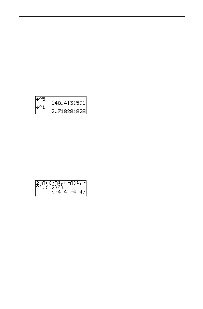
log, 10^, ln
x
ä
ã
10
), and
returns the value of the
e^1
(natural log
ln
e^
(logarithm «),
log
ä
ã
ln
) may be used with a number, expression, or list.
log
e^
e^
,
10^
value
power
(exponential y
returns the constant e raised to a power.
(power of ten y
10^
,
ln
value
x
ä
ã
e
) may be used with a number, expression, or list.
constant e.
e^
power
M
(Negation)
M
(negation Ì) returns the negative of a number, expression, list, or matrix
(Chapter 10). The narrow negation symbol (
the subtraction or minus ¹ (
M
value
EOS rules (Chapter 1) determine when negation is evaluated. For example,
2
M
returns a negative number (squaring is evaluated before negation
A
according to EOS rules). Use parentheses to square a negated number,
2
.
(MA)
N
).
M
) distinguishes negation from
y
abs
(absolute value) returns the absolute value of a number, expression,
abs
list, or matrix (Chapter 10).
abs
value
p
(Pi)
p
ä
ã
Pi is stored as a constant in the TI.82. Press y
to copy the symbol
the cursor location. The number 3.1415926535898 is used internally in
calculations.
2-4 Math, Angle, and Test Operations
p
to
Page 51

MATH MATH Operations
To display the MATH MATH menu, press . When you select an item from the
menu, the name is copied to the cursor location. Functions that are valid for lists
return a list calculated on an element-by-element basis.
MATH MATH Menu
MATH NUM HYP PRB
1:8Frac
2:8Dec
3
3:
3
‡
4:
x
‡
5:
6: fMin(
7: fMax(
8: nDeriv(
9: fnInt(
0: solve(
8
Frac
8
(display as fraction) displays an answer as the rational equivalent.
Frac
The answer may be a number, expression, list, or matrix. If it cannot be
simplified or the denominator is more than three digits, the decimal
equivalent is returned.
expression
8
Frac
Display answer as fraction
Display answer as decimal
Cube
Cube root
th
n
root
Minimum of a function
Maximum of a function
Numerical derivative
Function integral
Solution (root) of a function
8
is valid only at the end of an expression.
Frac
8
Dec
8
(display as decimal) displays an answer in decimal form.
Dec
valid only at the end of an expression.
expression
8
Dec
8
is
Dec
Math, Angle, and Test Operations 2-5
Page 52

3
(Cube)
3
(cube,
MATH MATH
item 3) returns the cube of a number, expression, list,
or square matrix (Chapter 10).
3
value
3
‡
(Cube Root)
3
‡
(cube root,
MATH MATH
item 4) returns the cube root of a number,
expression, or list.
3
value
‡
x
‡
(Root)
x
‡
(root,
MATH MATH
item 5) returns the
th
n
expression, or list.
x
th
n
root
value
‡
fMin(, fMax(
(function minimum,
fMin(
maximum,
MATH MATH
maximum value of
lower
and
tolerance
upper
and
fMax(
values for
are not valid in
(optional; if not specified, 1
MATH MATH
item 7) return the value at which the minimum or
expression
with respect to
variable. lower
expression
item 6) and
must be less than
. The accuracy is controlled by
.
E
5 is used). If there is no finite
minimum or maximum in the interval, usually (depending on
an error occurs.
expression,variable,lower,upper
fMin(
expression,variable,lower,upper,tolerance
fMin(
)
or
real root of a number,
(function
fMax(
variable
occurs, between
upper
expression
)
.
fMin(
)
2-6 Math, Angle, and Test Operations
Page 53

nDeriv(
(numerical derivative,
nDeriv(
derivative of
expression
MATH MATH
with respect to
item 8) returns an approximate
variable
, given the
to calculate the derivative, and H (optional; if none is specified, 1
used).
expression,variable,value
nDeriv(
expression,variable,value,H
nDeriv(
uses the symmetric difference quotient method, which
nDeriv(
or
)
)
approximates the numerical derivative value as the slope of the secant line
through the points:
value–H, expression(value–H
(
value+H,expression(value+H
(
)) and
))
As H gets smaller, the approximation usually gets more accurate.
value
at which
.
E
3 is
can be used once in
nDeriv(
expression
. Because of the method,
can return a false derivative value at a nondifferentiable point.
fnInt(
(function integral,
fnInt(
MATH MATH
(Gauss-Kronrod method) of
lower
limit,
upper
limit, and a
expression
item 9) returns the numerical integral
with respect to
tolerance
(optional; if none is specified, 1
is used).
expression,variable,lower,upper
fnInt(
expression,variable,lower,upper,tolerance
fnInt(
is not valid in
fnInt(
expression
or
)
.
Math, Angle, and Test Operations 2-7
nDeriv(
variable
)
, given
.
E
5
Page 54

solve(
(
solve(
variable
MATH MATH
, given an initial
item 0) returns a solution (root) of
guess
, a
lower
which a solution is sought (optional, if not specified,
upper
solve(
solve(
expression
not be updated.
stored to every variable in
is evaluated.
Controlling the Solution for solve(
E
99).
=1
expression,variable,guess
or
)
expression,variable,guess,{lower,upper
is assumed equal to zero. The value of
guess
may be a value or a list of two values. Values must be
expression
lower
and
upper
are entered in list format.
bound, and an
})
, except
variable
expression
upper
lower
variable
, before
The TI.82 solves equations through an iterative process. To control that
process, you should provide a close bound of the solution and at least one
initial guess (which must be within the bounds). This will help to:
¦
Find a solution.
¦
Define which solution you want for equations with multiple solutions.
¦
Find the solution more quickly.
for
bound within
E
99 and
=.1
in memory will
expression
2-8 Math, Angle, and Test Operations
Page 55

MATH NUM (Number) Operations
To display the MATH NUM menu, press
menu, the name is copied to the cursor location. Functions that are valid for lists
return a list calculated on an element-by-element basis.
MATH NUM Menu
MATH NUM HYP PRB
round(
iPart
1: round(
2: iPart
3: fPart
4: int
5: min(
6: max(
returns a number, expression, list, or matrix rounded to
round(
#decimals
(9). If
value,#decimals
round(
value
round(
iPart
)
(integer part) returns the integer part or parts of a number,
Round
Integer part
Fractional part
Greatest integer
Minimum value
Maximum value
is omitted,
)
~
. When you select an item from the
value
is rounded to 10 digits.
#decimals
expression, list, or matrix (Chapter 10).
value
iPart
fPart
(fractional part) returns the fractional part or parts of a number,
fPart
expression, list, or matrix (Chapter 10).
value
fPart
Math, Angle, and Test Operations 2-9
Page 56
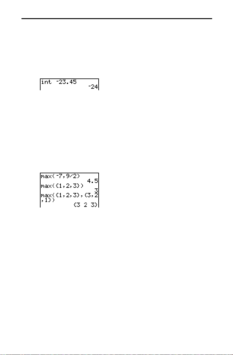
int
(greatest integer) returns the largest integer less than or equal to a
int
number, expression, list, or matrix. The value is the same as
nonnegative numbers and negative integers, but one integer less than
for negative noninteger numbers.
value
int
min(, max(
(minimum value) returns the smaller of
min(
valueA
or
valueB
smallest element in a list. If two lists are compared, it returns a list of the
smaller of each pair of elements.
(maximum value) returns the larger of
max(
valueA
or
valueB
element in a list. If two lists are compared, it returns a list of the larger of
each pair of elements.
valueA,valueB
min(
list
min(
listA,listB
min(
or
)
or
)
or
)
valueA,valueB
max(
list
max(
listA,listB
max(
)
)
)
for
iPart
iPart
or the
or the largest
Note: The
as the
min(
min(
and
and
max(
functions on the
max(
functions on the
2-10 Math, Angle, and Test Operations
MATH NUM
LIST MATH
menu are the same
menu.
Page 57

MATH HYP (Hyperbolic) Operations
To display the MATH HYP menu, press
~ ~
. When you select an item from
the menu, the name is copied to the cursor location. Functions that are valid for
lists return a list calculated on an element-by-element basis.
MATH HYP Menu
MATH NUM HYP PRB
1: sinh
2: cosh
3: tanh
4: sinh
5: cosh
6: tanh
–1
–1
–1
Hyperbolic sine
Hyperbolic cosine
Hyperbolic tangent
Hyperbolic arcsine
Hyperbolic arccosine
Hyperbolic arctangent
sinh, cosh, tanh
sinh, cosh
value
sinh
sinh–1, cosh–1, tanh
–1
,
sinh
cosh
, and
are the hyperbolic functions. They are valid for lists.
tanh
–1
–1
, and
–1
are the hyperbolic arcsine, hyperbolic arccosine,
tanh
and hyperbolic arctangent functions, respectively. They are valid for lists.
–1
value
sinh
Math, Angle, and Test Operations 2-11
Page 58

MATH PRB (Probability) Operations
To display the MATH PRB menu, press
menu, the name is copied to the cursor location. Functions that are valid for lists
return a list calculated on an element-by-element basis.
MATH PRB Menu
MATH NUM HYP PRB
rand
1: rand
2: nPr
3: nCr
4: !
(random number) generates and returns a random number greater
rand
Random number generator
Number of permutations
Number of combinations
Factorial
|
. When you select an item from the
than 0 and less than 1. A random number is generated from a seed value. To
control a random number sequence, first store an integer seed value in
rand
you reset the TI.82,
nPr
nPr
taken
items
nCr
nCr
items
. If you store 0 to
(number of permutations) returns the number of permutations of
number
at a time.
number
nPr
(number of combinations) returns the number of combinations of
number
taken
, the TI.82 uses the factory-set seed value. When
rand
is set to the factory seed.
rand
items
at a time.
and
items
number
must be nonnegative integers.
number
and
must be nonnegative
items
integers.
nCr
number
items
! (Factorial)
(factorial) returns the factorial of a positive integer between 0 and 69.
!
value
!
2-12 Math, Angle, and Test Operations
Page 59
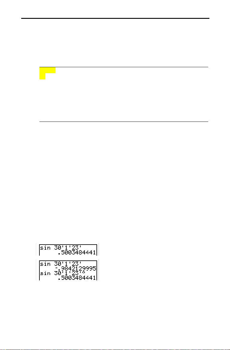
ANGLE Operations
y
To display the ANGLE menu, press
indicators and instructions. When you select an item from the menu, the name is
copied to the cursor location. Angle entries are interpreted according to the
Radian/Degree MODE setting.
ANGLE Menu
ANGLE
¡
1:
2: '
r
3:
4:8DMS
5: R8Pr(
6: R8Pq(
7: P8Rx(
8: P8Ry(
Degree function
DMS entry notation
Radian function
Display as degree/minute/second
Returns R, given X and
Returns q, given X and
Returns X, given R and
Returns Y, given R and
;
. The ANGLE menu displays angle
Y
Y
q
q
Note: Do not enter DMS numbers as
54¡32'30"
interpreted as implied multiplication of 54
on the TI.82.
¡
and 32', and " is a quote mark
used to enter text.
¡
(Degree)
¡
(degree) lets you designate
setting.
MODE
angle
¡
' (DMS Entry Notation)
(DMS entry notation) lets you enter degrees, minutes, and seconds in DMS
'
angle
may be a list.
angle
as degree, regardless of the current angle
format.
degrees
For example, enter
the
minutes'seconds
'
setting must be
MODE
'
for 30 degrees, 1 minute, 23 seconds. Note that
30'1'23'
(or you must use the
Degree
for the TI.82 to interpret the argument as degrees, minutes, and seconds.
Degree
MODE
Radian
MODE
r
(Radians)
r
(radian) lets you designate
MODE
angle
setting.
r
angle
may be a list.
angle
as radian, regardless of the current angle
Degree
54¡32'
function)
is
Math, Angle, and Test Operations 2-13
Page 60

8
DMS
8
(display as degree/minute/second) displays
DMS
minute, second format. The
interpret
answer
as degrees, minutes, and seconds.
the end of a line.
answer
8
DMS
R8Pr(, R8Pq(, P8Rx(, P8Ry(
converts rectangular to polar and returns R, and
R8Pr(
rectangular to polar and returns
values.
R8Pr(X,Y)
X,Y
R8Pq(
)
answer
in degree,
setting must be
MODE
q
, given X and Y rectangular coordinate
Degree
8
DMS
R8Pq(
for the TI.82 to
is valid only at
converts
converts polar to rectangular and returns X, and
P8Rx(
polar to rectangular and returns
P8Rx(R,q)
R
P8Ry(
,q)
, given R and q polar coordinate values.
Y
2-14 Math, Angle, and Test Operations
P8Ry(
converts
Page 61

TEST TEST (Relational) Operations
y
To display the TEST TEST menu, press
the name is copied to the cursor location. These functions are valid for lists; they
return a list calculated on an element-by-element basis.
TEST TEST Menu
TEST LOGIC
1: =
ƒ
2:
3: >
‚
4:
5: <
6:
True if:
Equal
Not equal to
Greater than
Greater than or equal to
Less than
Less than or equal to
:
. When you select from the menu,
=, ƒ, >, ‚, <,
Relational operators compare
true or
if the test is false.
0
valueA
valueA
and
and
valueB
valueB
and return 1 if the test is
can be numbers,
expressions, lists, or matrices (Chapter 10), but they must match in type
and dimension. Relational operators are often used in programs to control
program flow and in graphing to control the graph of a function over
specific values.
valueA
Using Tests
valueB
=
Relational operators are evaluated after mathematical functions according
to EOS rules (Chapter 1).
¦
The expression
2+2=2+3
returns 0. The TI.82 does the addition first
because of EOS rules, and then it compares 4 to 5.
¦
The expression
2+(2=2)+3
returns 6. The TI.82 first performs the
relational test because it is in parentheses, and then it adds 2, 1, and 3.
Math, Angle, and Test Operations 2-15
Page 62

TEST LOGIC (Boolean) Operations
y
To display the TEST LOGIC menu, press
menu, the name is copied to the cursor location.
TEST LOGIC Menu
TEST LOGIC
1: and
2: or
3: xor
4: not
Boolean Operators
True if:
Both values are nonzero (true)
At least one value is nonzero (true)
Only one value is zero (false)
The value is zero (true)
Boolean operators are often used in programs to control program flow and
in graphing to control the graph of a function over specific values. Values
are interpreted as zero (false) or nonzero (true).
and, or, xor
, and
and, or
if the expression is false, according to the table below.
0
(exclusive or) return a value of 1 if a expression is true or
xor
can be expressions.
:
~. When you select from the
valueA
and
valueB
valueA
valueA
valueA
valueA
valueB
and
valueB
or
valueB
xor
valueB
ƒ
0
ƒ
0 0 returns 0 1 1
0
ƒ
0 returns 1 1 0
ƒ
0 returns 0 1 1
and or xor
0 0 returns 0 0 0
not
returns 1 if
not
value
not
Using Boolean Operations
value
(which can be an expression) is 0.
Boolean logic is often used with relational tests. In a program, the following
instructions store
into C:
4
2-16 Math, Angle, and Test Operations
Page 63

Chapter 3: Function Graphing
This chapter describes function graphing on the TI.82 in detail. It also lays the
foundation for using the other graphing features of the TI.82.
Chapter Contents
Getting Started: Graphing a Circle
Defining a Graph
Setting Graph Modes
Defining Functions in the
Selecting Functions
Defining the Viewing
Setting
WINDOW FORMAT
Displaying a Graph
...............................
............................
Y=
.............................
WINDOW
........................
.............................
Exploring a Graph with the Free-Moving Cursor
Exploring a Graph with
Exploring a Graph with
Using
ZOOM MEMORY
Setting
ZOOM FACTORS
Using
(Calculate) Operations
CALC
TRACE
ZOOM
..........................
.........................
..................
...................
List
....................
........
....................
.....................
.................
3-10
3-11
3-13
3-14
3-16
3-19
3-20
3-21
3-2
3-3
3-4
3-5
3-7
3-8
Function Graphing 3-1
Page 64
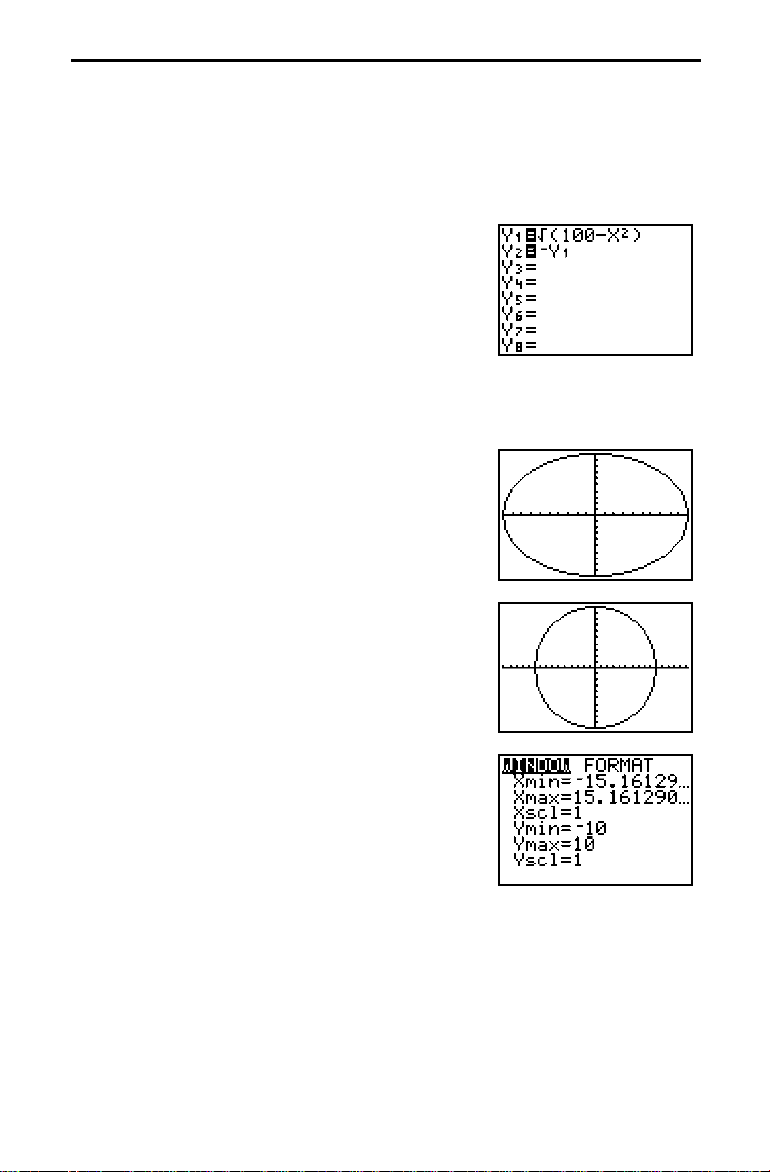
Getting Started: Graphing a Circle
Getting Started is a fast-paced introduction. Read the chapter for details.
Graph a circle of radius 10, centered on the origin in the standard viewing
window. To graph a circle, you must enter separate formulas for the upper and
lower portions of the circle. Then use ZOOM Square to adjust the display to make
the functions appear as a circle.
1. In
Func
, press o to display the Y= edit
MODE
screen. Press y
‡
ã
ä
£
„ ¡ ¤ Í
¹
100
to enter the expression to define the top half of
the circle,
Y1=‡(100–X2)
.
The bottom half of the circle is defined by
Y2=M‡(100–X2)
. However, on the TI.82 you can
define one function in terms of another, so to
ä
define
the
Y=
(to select
2. Press
1
, press Ì y
Y2=MY
variables menu) 1 (to select
1
).
Y
q
and then select
quick way to reset the
ã
Y.VARS
ZStandard
WINDOW
(to display
Function...) 1
. This is a
variables to the
standard values. It also graphs the functions; you
do not need to press
s
.
Notice that the functions appear as an ellipse in
the standard viewing window.
3. To adjust the display so each “dot” represents an
equal width and height, press
select
ZSquare
. The functions are replotted and
q
and then
now appear as a circle on the display.
4. To see the effect of
variables, press
values for
p
Xmin, Xmax, Ymin
ZSquare
on the
WINDOW
and notice the new
, and
Ymax
.
3-2 Function Graphing
Page 65

Defining a Graph
To define a graph, you set the modes, enter and select the functions to graph,
and define the viewing WINDOW and WINDOW FORMAT. Once you have defined
a graph, you can plot, display, and explore it.
Steps in Defining a Graph
There are six basic steps to defining a graph. You may not need to do all the
steps each time you define a graph. The procedures are described in detail
on the following pages.
1. Set the
2. Enter or edit a function in the Y= list.
3. Select the Y= function you want to graph.
4. Define the viewing
5. Set the
6. Deselect stat plots, if appropriate (Chapter 12.)
Exploring a Graph
Once you have defined a graph, you can display it and then use several
tools of the TI.82 to explore the behavior of the function or functions.
These tools are described later in this chapter.
Saving a Graph
You can store the elements that define the current graph in one of six graph
databases (Chapter 8). Later, you can recall that database to recreate the
current graph.
You can store a picture of the current graph display in one of six graph
pictures (Chapter 8). Later, you can superimpose that picture on the
current graph.
to
MODE
WINDOW FORMAT
Func
WINDOW
graphing.
variables.
.
Function Graphing 3-3
Page 66

Setting Graph Modes
Pressing z displays the current MODE settings (Chapter 1). The graphing
MODE in function graphing must be Func.
Checking and Changing Graphing Modes
Press z to display the
highlighted.
The TI.82 has four graphing modes.
¦
¦
¦
¦
(function graphing)
Func
(parametric graphing)
Par
(polar graphing)
Pol
(sequence graphing)
Seq
To graph functions, you must select
of graphing on the TI.82 are described in this chapter. Differences in
parametric graphing (Chapter 4), polar graphing (Chapter 5), and sequence
graphing (Chapter 6) are described in those chapters.
or
Radian
Connected
Sequential
Degree
MODE
or
affects how the selected functions are plotted.
Dot
or
affects how functions are plotted if you have more
Simul
than one function selected.
Setting Modes from a Program
You may set the graphing mode and other modes from a program.
Begin on a blank line in the program editor. Press z to display the
interactive
on the
MODE
is copied to the cursor location.
MODE
selection screen. Use †, }, ~, and | to place the cursor
MODE
that you want to select, and press
settings. The current settings are
MODE
(function graphing). The basics
Func
may affect how some functions are interpreted.
. The name of the
Í
3-4 Function Graphing
Page 67

Defining Functions in the Y= List
Pressing o accesses the Y= edit screen, where you enter the functions to graph.
You can store up to ten functions in memory at one time. You can graph one or
more of these functions at a time.
Displaying the Functions in the Y= List
Press o to display the Y= edit screen. In the example below, the
functions are defined.
Defining a New Function
To define a new function, enter an expression on the Y= edit screen.
1. Move the cursor to the function in the Y= list you want to define. If
necessary, press
to erase a previously entered function.
‘
2. Enter the expression to define the function.
¦
You may use functions and variables (including matrices and lists) in
the expression. If the expression evaluates to a value that is not a
real number, that point is not plotted; an error does not occur.
¦
The independent variable in the function is X. You may press
ã
ä
rather than pressing
ƒ
X
, for the
variable. (
X
defines the independent variable as X.)
¦
The expression is stored as one of the ten user-defined functions in
the
list as you enter it.
Y=
3. When you complete the expression, press
to move to the
Í
beginning of the next function.
Func
Y
MODE
1
and
„
Y
,
2
Function Graphing 3-5
Page 68
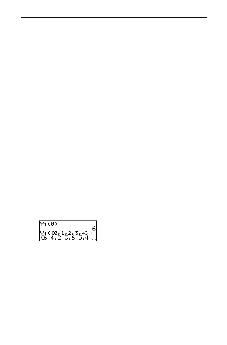
Editing a Function
1. Move the cursor to the function in the Y= list you want to change.
2. Make the changes. You can press
‘
to erase the expression and
then enter a new expression.
The expression is stored as one of the ten user-defined functions in the
list as you enter it.
Clearing a Function
To clear or erase a function on the Y= edit screen, position the cursor
anywhere on the function, and then press
Defining Functions from the Home Screen or a Program
1. Begin on a blank line. Press
ã
ä
"
ƒ
press
again.
ƒ
‘
.
ä
ã
"
, enter the expression, and then
2. Press ¿.
ã
ä
3. Press y
Y.VARS
, select
Function...
, and then select the name of the
function, which is copied to the cursor location.
4. Press
Í
expression
"
to complete the instruction.
n
"!Y
When the instruction is executed, the TI.82 stores the expression to the
list, selects the function, and displays the message
Evaluating Y= Functions in Expressions
Done
You can the calculate the value of a Y= function at a specified value of X.
For example, if
Y1=.2X3–2X+6
:
Y=
Y=
.
3-6 Function Graphing
Page 69

Selecting Functions
Only functions that are selected are graphed. Up to ten functions may be selected
at one time.
Turning a Function “On” or “Off”
You select and deselect (“turn on” and “turn off”) functions on the Y= edit
screen. The = sign on a selected function is highlighted. To change the
selection status of a function:
1. If the
2. Move the cursor to the function whose status you want to change.
3. Use | to place the cursor over the = sign of the function.
4. Press
Note: When you enter or edit a function, it is selected automatically. When
you clear a function, it is deselected.
Leaving the Y= Edit Screen
To leave the Y= edit screen:
¦
Select another screen by pressing the appropriate key, such as
or
¦
Press y
Selecting Functions from the Home Screen or a Program
1. Begin on a blank line. Press y
ON/OFF
2. Select the instruction you want,
cursor location.
3. If you want to turn specific functions on or off, enter the number of the
function(s), separated by commas.
When the instruction is executed, the status of each function in the current
graph mode is set appropriately and
FnOn
FnOff
FnOn
FnOff
For example, in
list and then turns on
Y=
edit screen is not displayed, press o to display the functions.
Y=
Í
to change the status.
p
.
ä
ã
QUIT
to return to the Home screen.
ä
ã
Y.VARS
and select
On/Off...
menu is displayed.
function1,function2
function1,function2
Func
MODE
. . .
,
. . .
,
,
FnOff:FnOn 1,3
1
3
and
Y
Y
FnOn
Done
.
or
is displayed.
. It is copied to the
FnOff
turns off all functions in the
s
. The
Function Graphing 3-7
Page 70

Defining the Viewing
The WINDOW variables determine the boundaries and other attributes of the
viewing WINDOW. The WINDOW variables are shared by all graphing modes.
TI-82 Viewing WINDOW
The viewing
defined by
is defined by
WINDOW
WINDOW
Xmin, Xmax, Ymin
Xscl
of the TI.82 is the portion of the coordinate plane
for the X axis and
Ymax
, and
. The distance between tick marks
Ymax
for the Y axis.
Yscl
Xmin
Checking the Viewing WINDOW
p
Press
Xscl
Xmax
Yscl
Ymin
to display the current
WINDOW
variable values. The values
shown here are the standard values.
Changing a WINDOW Variable Value
1. Press † to move to the
WINDOW
variable you want to change.
2. To enter a real value (which can be an expression), you may do any of
the following:
¦
Position the cursor and then make the changes.
¦
¦
‘
Press
to clear the value and then enter a new value.
Begin entering a new value. The original value is cleared
automatically when you begin typing.
3. Press
Í, †
, or }. If you entered an expression, it is evaluated. The
new value is stored.
must be less than
Xmin
get an error message when you press
Xscl=0
or
Yscl=0
.
Xmax
and
must be less than
Ymin
s
. To turn off the tick marks, set
Ymax
, or you will
3-8 Function Graphing
Page 71

Leaving the WINDOW Edit Screen
To leave the
¦
Select another screen by pressing the appropriate key, such as
WINDOW
edit screen:
or o.
ä
¦
Press y
Storing to a WINDOW Variable from the Home Screen or a Program
ã
QUIT
to return to the Home screen.
Begin on a blank line.
1. Enter the value you want to store (which can be an expression).
2. Press ¿.
3. Press
4. Select
5. Select the
to display the
Window...
WINDOW
menu.
VARS
to display the
WINDOW
variables.
variable to which you want to store. The name of
the variable is copied to the cursor location where you are editing.
6. Press
Í
to complete the instruction.
When the instruction is executed, the TI.82 stores the value in the
WINDOW
Note: You can use a
variable.
WINDOW
variable in an expression by performing
steps 3, 4, and 5.
@
X and @Y
@
The variables
X
@
and
define the distance between the centers of two
Y
adjoining pixels on a graph (graphing accuracy).
(
–
@
=
X
Xmax
)(
Xmin
@
=
Y
Ymax
–
Ymin
)
94 62
s
@
@
and
X
VARS Window
Ymax
are not on the
Y
menu.
@
and
X
WINDOW
@
when a graph is displayed.
You can store values directly to
are calculated from
@
,
,
X
Xmin
screen; they are accessible through the
are calculated from
Y
@
@
X
, and
Y
and
@
Ymin
, in which case
Y
immediately.
Xmin, Xmax, Ymin
Xmax
Function Graphing 3-9
and
, and
Ymax
Page 72

Setting WINDOW FORMAT
WINDOW FORMAT determines how a graph appears on the display. WINDOW
FORMAT settings apply to all graphing modes.
Checking WINDOW FORMAT
To display the
WINDOW FORMAT
screen, press
settings are highlighted.
WINDOW FORMAT
RectGC PolarGC
CoordOn CoordOff
GridOff GridOn
AxesOn AxesOff
LabelOff LabelOn
Changing WINDOW FORMAT
Sets rectangular or polar cursor.
Sets cursor coordinates on or off.
Sets grid off or on.
Sets axes on or off.
Sets axes label off or on.
1. Move the cursor to the row of the setting you want to change. The
setting the cursor is on blinks.
2. Move the cursor to the setting you want and press
RectGC, PolarGC
The cursor coordinate setting determines if the cursor location is displayed
(if
CoordOn
) as rectangular coordinates X and Y or polar coordinates
and q. It also determines which variables are updated. In
(rectangular graphing coordinates)
FORMAT
the free-moving cursor, or tracing updates and displays
(polar graphing coordinates)
FORMAT
, X, Y, R, and q are updated, and
and q are displayed.
p ~
. The current
Í
.
RectGC
, plotting the graph, moving
and Y. In
X
PolarGC
R
R
CoordOn, CoordOff
CoordOn
(coordinates on) displays the function number in the upper-right
corner and the cursor coordinates at the bottom of the graph.
(coordinate off) does not display the function number or the coordinates
for the free-moving cursor or during
GridOff, GridOn
Grid points correspond to the axis tick marks.
points.
AxesOn, AxesOff
AxesOn
does display the grid points.
GridOn
displays the axes.
AxesOff
does not display the axes. It overrides
TRACE
.
does not display grid
GridOff
the Axis Label setting.
LabelOff, LabelOn
LabelOn
and
LabelOff
determine whether to display a label for the axes (
and Y).
3-10 Function Graphing
CoordOff
X
Page 73

Displaying a Graph
Pressing
MODE settings apply, and the current values of the WINDOW variables define the
viewing WINDOW.
Displaying a New Graph
s
graphs any functions selected on the Y= edit screen. The current
Press
to display the graph of the selected function or functions.
s
(Some operations, such as
TRACE
and the
ZOOM CALC
operations, display
the graph automatically.) As a graph is plotted, the busy indicator is on and
and Y are updated.
X
Pausing a Graph
Note: While a graph is being plotted, you can:
¦
¦
Smart Graph
When you press
Press
Press É to stop graphing, then press
to pause graphing, then press
Í
, Smart Graph displays the graph screen
s
Í
s
to resume plotting.
to start over.
immediately if nothing has changed that requires the functions to be
replotted since the last time the graph was displayed.
If you have not changed any of the following since the graph was last
displayed, Smart Graph displays the graph immediately. If you have
changed one or more of these, pressing
replots the graph based on
s
the new values.
¦
Changed a
¦
Changed a function.
¦
Selected or deselected a function.
¦
Changed the value of a variable in a selected function.
¦
Changed a
¦
Cleared drawings by selecting
¦
Changed a
setting that affects graphs.
MODE
WINDOW
STAT PLOT
variable or a
definition (Chapter 12).
FORMAT
ClrDraw
setting.
(Chapter 8).
Function Graphing 3-11
Page 74

Graphing a Family of Curves
If you enter a list (Chapter 11) as an element in an expression, the TI.82
plots the function for each value in the list, graphing a family of curves. (In
, it graphs all functions for the first element, and so on.)
Simul
{2,4,6}sin X
graphs three functions:
2 sin X, 4 sin X
, and
6 sin X
.
{2,4,6}sin {1,2,3}X
graphs
2 sin X, 4 sin 2X
, and
6 sin 3X
.
3-12 Function Graphing
Page 75

Exploring a Graph with the Free-Moving Cursor
While a graph is displayed, you can move the free-moving cursor anywhere on
the graph and display the coordinates of any location on the graph.
Free-Moving Cursor
You can use |, ~, }, or † to move the cursor around the graph. When you
first display the graph, no cursor is visible. As soon as you press |, ~, },
or †, the cursor moves from the center of the viewing window.
As you move the cursor around the graph, the coordinate values of the
cursor location are displayed at the bottom of the screen (if
Coordinate values generally appear in normal floating-decimal format. The
numeric display settings on the
screen do not affect coordinate
MODE
display.
To see the graph without the cursor or coordinate values, press
Í
. When you press |, ~, }, or †, the cursor moves from same
position.
Graphing Accuracy
The free-moving cursor moves from dot to dot on the screen. When you
move the cursor to a dot that appears to be “on” the function, it may be
near, but not on, the function; therefore, the coordinate value displayed at
the bottom of the screen is not necessarily a point on the function. To move
the cursor along a function, use
TRACE
(page 3.14).
The display coordinate values of the free-moving cursor approximate actual
math coordinates accurate to within the width/height of the dot. As
and
Xmax
(and
Ymin
and
) get closer together (after a
Ymax
example), graphing accuracy increases, and the coordinate values more
closely approximate the math coordinates.
CoordOn
Zoom In
).
‘
Xmin
, for
or
Free-moving cursor “on” the curve
)
Function Graphing 3-13
Page 76

Exploring a Graph with TRACE
TRACE moves the cursor from one plotted point to the next along a function,
while displaying the cursor coordinates at the bottom of the screen.
Beginning a Trace
r
Press
displays it. The cursor is on the first selected function in the
middle
upper right of the display.
Moving along a Function
~
and | move the cursor along the function. Each press moves the cursor
from one plotted point to the next. y ~ and y | move the cursor five
plotted points at a time. The
Y=Yn(X)
to begin a trace. If the graph is not displayed already, the TI.82
list at the
value on the screen. The number of the function shows at the
X
value is calculated from the X value; that is,
Y
Y=
. If the function is undefined at an X value, the Y value is blank.
)
cursor on the curve.
TRACE
If the Y value of a function is above or below the viewing window, the
cursor disappears as you move it to that portion of the function; however,
the coordinate values at the bottom of the screen indicate the cursor
coordinates.
Panning to the Left or Right
If you trace a function off the left or right edge of the screen, the viewing
window automatically pans to the left or right.
Xmin
and
to correspond to the new viewing window.
QuickZoom
While tracing, you can press
Í
to adjust the viewing
the cursor location becomes the center of the new viewing
if the cursor is above or below the display. This allows “panning” up and
down. After QuickZoom, the cursor remains in
TRACE
.
are updated
Xmax
WINDOW
WINDOW
so that
, even
3-14 Function Graphing
Page 77

Moving from Function to Function
To trace another selected function on the graph, use † or } to move the
cursor to that function. The cursor movement is based on the order of the
selected functions in the
list, not the appearance of the functions as
Y=
graphed on the screen. The cursor moves to the new function at the same
value. The function number in the upper right corner of the display
changes.
Leaving TRACE
To leave
¦
Select another screen by pressing the appropriate key, such as
q
or
¦
Press y
The
TRACE
:
TRACE
.
ä
ã
QUIT
to return to the Home screen.
cursor remains in the same location if you leave
return, if Smart Graph has not caused the graph to be replotted.
Using TRACE in a Program
On a blank line in the program editor, press
r
. The instruction
copied to the cursor location. When the instruction is encountered during
program execution, the graph is displayed with the
TRACE
first selected function. As you trace, the cursor coordinate values are
updated. When you are done tracing functions, press
Í
program execution.
p
and
TRACE
Trace
cursor on the
to resume
X
is
Function Graphing 3-15
Page 78

Exploring a Graph with ZOOM
Pressing
of the graph quickly in a variety of ways. All of the ZOOM commands are
accessible from programs.
ZOOM Menu
ZBox
q
accesses a menu that allows you to adjust the viewing WINDOW
ZOOM MEMORY
1: ZBox
2: Zoom In
3: Zoom Out
4: ZDecimal
5: ZSquare
6: ZStandard
7: ZTrig
8: ZInteger
9: ZoomStat
lets you use the cursor to select opposite corners of a box to define a
ZBox
new viewing
1. Select
the screen indicates that you are using a
Draws box to define viewing
Magnifies graph around cursor.
Views more of graph around cursor.
Sets .1 as dot size.
Sets equal sized dots on X and Y axes.
Sets standard
Sets built-in trig
WINDOW
WINDOW
Sets integer values on X and Y axes.
Sets values for current lists.
WINDOW
ZBox
.
from the
menu. The different cursor at the center of
ZOOM
WINDOW
variables.
variables.
ZOOM
.
instruction.
2. Move the cursor to any corner of the box you want to define and then
press
. As you move the cursor away from the point just selected,
Í
you see a small square dot, indicating that the first corner is selected.
3. Move the cursor to the diagonal corner of the box you want to define.
As you move the cursor, the boundaries of the box change on the
screen.
Note: You can cancel
pressing
‘
.
any time before you press
ZBox
4. When the box is defined as you want it, press
You can repeat steps 2 through 4 to do another
press
‘
.
3-16 Function Graphing
Í
ZBox
by
Í
to replot the graph.
. To cancel
ZBox
,
Page 79

Zoom In, Zoom Out
Zoom In
magnifies the graph around the cursor location.
displays a greater portion of the graph, centered on the cursor location, to
provide a more global view. The
XFact
and
settings determine the
YFact
extent of the zoom.
1. After checking or changing
from the
ZOOM
menu.
XFact
and
(page 3.20), select
YFact
Notice the different cursor. It indicates that you are using a
instruction.
2. Move the cursor to the point that you want as the center of the new
viewing
WINDOW
, then press
The TI.82 adjusts the viewing
the
WINDOW
variables, and replots the selected functions, centered on
Í
.
WINDOW
by
XFact
and
the cursor location.
3. To zoom in on the graph again:
Zoom Out
The procedure for
¦
To zoom in at the same point, press
¦
To zoom in at a new point, move the cursor to the point that you
want as the center of the new viewing
Í
.
Zoom Out
is the same as for
Í
WINDOW
.
Zoom In
and then press
.
Zoom Out
ZOOM
, updates
YFact
Zoom In
Leaving Zoom In or Zoom Out
To leave
¦
Zoom In
Select another screen by pressing the appropriate key, such as
s
¦
Press y
or
.
ä
ã
QUIT
to return to the Home screen.
Zoom Out
:
r
or
Function Graphing 3-17
Page 80

ZDecimal
ZDecimal
variables to preset values that set
replots the functions immediately, updating the
@
@
and
X
equal to .1 and defining the
Y
and Y value of each pixel as one decimal.
Xmin = M4.7 Ymin = M3.1
Xmax = 4.7 Ymax = 3.1
Xscl = 1 Yscl = 1
ZSquare
ZSquare
on the current
that
Yscl
replots the functions immediately, redefining the
@X=@
WINDOW
. This makes the graph of a circle look like a circle.
Y
variables, but adjusted in only one direction so
remain unchanged. The midpoint of the current graph (not the
intersection of the axes) becomes the midpoint of the new graph.
ZStandard
ZStandard
replots the functions immediately, updating the
variables to the standard values:
Xmin = M10 Ymin = M10
Xmax = 10 Ymax = 10
Xscl = 1 Yscl = 1
ZTrig
replots the functions immediately, updating the
ZTrig
preset values appropriate for trig plotting functions. In
are:
Xmin = M(47à24)
Xmax = (47à24)
Xscl = p/2 Yscl = 1
p
p
Ymin = M4
Ymax = 4
WINDOW
WINDOW
WINDOW
WINDOW
Radian
based
and
Xscl
variables to
these
MODE
X
ZInteger
ZInteger
Yscl=10
redefines the viewing
, replotting the functions after you move the cursor to the point that
you want as the center of the new
ZoomStat
ZoomStat
redefines the viewing
WINDOW
WINDOW
WINDOW
@
so
X=1
and
and press
so that all statistical data points
are displayed. For one-variable plots (histograms and box plots), only
and
TRACE
are adjusted. If the top of the histogram is not shown, use
Xmax
to determine the value for
Ymax
.
3-18 Function Graphing
@
Y=1
Í
,
Xscl=10
.
, and
Xmin
Page 81

Using ZOOM MEMORY
ZPrevious allows you to return to the WINDOW displayed prior to the previous
ZOOM. ZoomSto stores the values of the current WINDOW variables to userdefined ZOOM MEMORY variables. ZoomRcl changes the WINDOW to the values
stored with ZoomSto.
ZOOM MEMORY Menu
ZOOM MEMORY
1: ZPrevious
2: ZoomSto
3: ZoomRcl
4: SetFactors
ZPrevious
When you select
replotted using the
previous
ZoomSto
ZOOM
To store the current viewing
ZOOM MEMORY
of the current
variables:
ZXmin, ZXmax, ZXscl, ZYmin, ZYmax
immediate, there is no prompting on the display.
These variables are global; they apply to all graphing modes. For example,
changing the value of
The user-defined
store to them the first time.
Uses previous viewing
Stores user-defined
Recalls user-defined
…
Changes
WINDOW
from the
variables of the graph displayed prior to the
ZPrevious
WINDOW
WINDOW
WINDOW
Zoom In, Zoom Out
ZOOM MEMORY
.
.
.
factors.
menu, the graph is
that you did.
WINDOW
, select
ZoomSto
from the
menu. The graph is displayed if necessary, and the values
WINDOW
variables are stored in the user-defined
, and
ZXmin
WINDOW
in
variables contain the standard values until you
Func
also changes it in
MODE
. The action is
ZYscl
ZOOM
Par
MODE
.
ZoomRcl
To view the selected graphing functions in the user-defined
select
ZoomRcl
from the
ZOOM MEMORY
menu. The
WINDOW
are updated with the user-defined values, and the graph is plotted.
Using ZOOM MEMORY from the Home Screen or a Program
From the Home screen or a program, you can store directly to any of the
user-defined
From a program, you can select the
the
ZOOM MEMORY
ZOOM
variables.
menu.
ZoomSto
or
ZoomRcl
Function Graphing 3-19
WINDOW
,
variables
instructions from
Page 82

Setting ZOOM FACTORS
The ZOOM FACTORS, XFact and YFact, determine the extent of the change for
the viewing window created by Zoom In or Zoom Out on a graph.
ZOOM FACTORS
ZOOM FACTORS
than or equal to 1. They define the magnification or reduction factor used
to
Zoom In
Checking XFact and YFact
To review the current values of
the
ZOOM MEMORY
values shown are the standard values).
Changing XFact and YFact
To change
¦
Enter a new value. The original value is cleared automatically when you
begin typing.
¦
Position the cursor over the digit you want to change. Then type over it
or use { to delete it.
are positive numbers (not necessarily integers) greater
or
Zoom Out
XFact
menu. The
or
YFact
around a point.
and
XFact
ZOOM FACTORS
:
, select
YFact
screen appears (the
SetFactors...
from
Leaving ZOOM FACTORS
To leave
¦
¦
ZOOM FACTORS
Select another screen by pressing the appropriate key, such as
q
or
Press y
.
ã
QUIT
3-20 Function Graphing
:
ä
to return to the Home screen.
p
Page 83

Using CALC (Calculate) Operations
ä
ã
Pressing y
to analyze the current graph functions. You are prompted to specify the
function(s), interval, and point.
CALCULATE Menu
CALCULATE
1: value
2: root
3: minimum
4: maximum
5: intersect
6: dy/dx
7:‰f(x)dx
value
value
1. Select
(above
CALC
evaluates currently selected functions for a specified value of X.
value
a prompt for you to enter
2. Enter a real value for X between
expression). Note: When there is a value entered for
the value; when there is no value,
3. Press
Í
at the entered
have selected
r
) accesses a menu with operations you can use
Calculates function value for given X.
Finds root of function.
Finds minimum of function.
Finds maximum of function.
Finds intersection of functions.
Finds numeric derivative of function.
Finds numeric integral of function.
from the
menu. The current graph is displayed, with
CALC
.
X
Xmin
‘
and
cancels
(which can be an
Xmax
value
,
X
.
‘
. The result cursor is on the first selected function in the list
and the coordinate values are displayed (even if you
X
CoordOff
on the
WINDOW FORMAT
screen).
4. Press † or } to move the cursor between functions at the entered
value. When | or ~ are pressed, the free-moving cursor appears. It
cannot necessarily move back to the
value.
X
clears
X
Function Graphing 3-21
Page 84

root
(
CALC
item 2) uses
root
-intercept) of a function. Selecting good values for the bounds and a guess
X
(Chapter 2) to find the root (zero or
solve(
help it find the correct root and find it more quickly.
1. Select
prompt to enter
root
from the
Lower Bound
menu. The current graph is displayed, with a
CALC
.
2. Use † or } to move the cursor to the function for which you want to
find the root.
3. Move the cursor to the
interval and press
value you want for the lower bound of the
X
Í
4
. A
indicator at the top of the display shows
the lower bound.
4. Set the upper bound in the same way. An indicator shows the upper
bound.
5. You are prompted for a
to help the TI.82 find the correct root
Guess
and to find it more quickly.
6. Use | or ~ to move the cursor to a point near the root of the function,
between the bounds. Press
Í
.
The result cursor is on the solution and the coordinate values are displayed
(even if you have selected
CoordOff
on the
WINDOW FORMAT
When you press |, ~, }, or †, the free-moving cursor appears.
3-22 Function Graphing
screen).
Page 85

minimum, maximum
(
minimum
CALC
item 3) and
maximum
(
item 4) find the minimum or
CALC
maximum of a function in a specified interval to a tolerance of 1
1. Select
minimum
or
maximum
from the
menu. The current graph
CALC
is displayed.
2. Set
Lower Bound, Upper Bound
, and
as described for
Guess
The result cursor is on the solution and the coordinate values are displayed
(even if you have selected
CoordOff
on the
WINDOW FORMAT
When you press |, ~, }, or †, the free-moving cursor appears.
intersect
(
intersect
item 5) uses
CALC
(Chapter 2) to find the intersection of
solve(
two functions. The intersection must appear on the display.
1. Select
intersection
and you are prompted to select the
from the
menu. The current graph is displayed
CALC
First curve
.
L
5.
E
.
root
screen).
2. Use † or } to move the cursor to the first function and press
3. Use † or } to move the cursor to the second function and press
Í
Í
.
The result cursor is on the solution and the coordinate values are displayed
(even if you have selected
CoordOff
on the
WINDOW FORMAT
screen).
When you press |, ~, }, or †, the free-moving cursor appears.
Function Graphing 3-23
.
Page 86

dy/dx
(numerical derivative,
dy/dx
(slope) of a function at a point with H = 1
1. Select
dy/dx
from the
CALC
item 6) finds the numerical derivative
CALC
L
E
3.
menu. The current graph is displayed.
2. Move the cursor to the X value at which you want to calculate the
derivative and press
Í
.
The result cursor is on the solution and the coordinate values are displayed
(even if you have selected
CoordOff
on the
WINDOW FORMAT
When you press |, ~, }, or †, the free-moving cursor appears.
‰
f(x)dx
‰
(numerical integral,
f(x)dx
function a specified interval. It uses the
L
E
1
3.
1. Select
‰
from the
f(x)dx
a prompt to enter
Lower Bound
item 7) finds the numerical integral of a
CALC
menu. The current graph is displayed, with
CALC
function, with a tolerance of
fnInt(
.
2. Use † or } to move the cursor to the function for which you want to
calculate the integral.
3. Set
Lower Limit
and
Upper Limit
as described for
root
.
The integral value is displayed and the integrated area is shaded. When you
press |, ~, }, or †, the free-moving cursor appears.
screen).
Note: The shaded area is a drawing. Use
invokes Smart Graph to clear the shaded area. (Chapter 8)
3-24 Function Graphing
ClrDraw
or any change that
Page 87

Chapter 4: Parametric Graphing
This chapter describes how to graph parametric equations on the TI.82. Before
doing parametric graphing, you should be familiar with Chapter 3, Function
Graphing.
Chapter Contents
Getting Started: Path of a Ball
Defining and Displaying a Parametric Graph
Exploring a Parametric Graph
.....................
...........
.....................
4-2
4-3
4-6
Parametric Graphing 4-1
Page 88
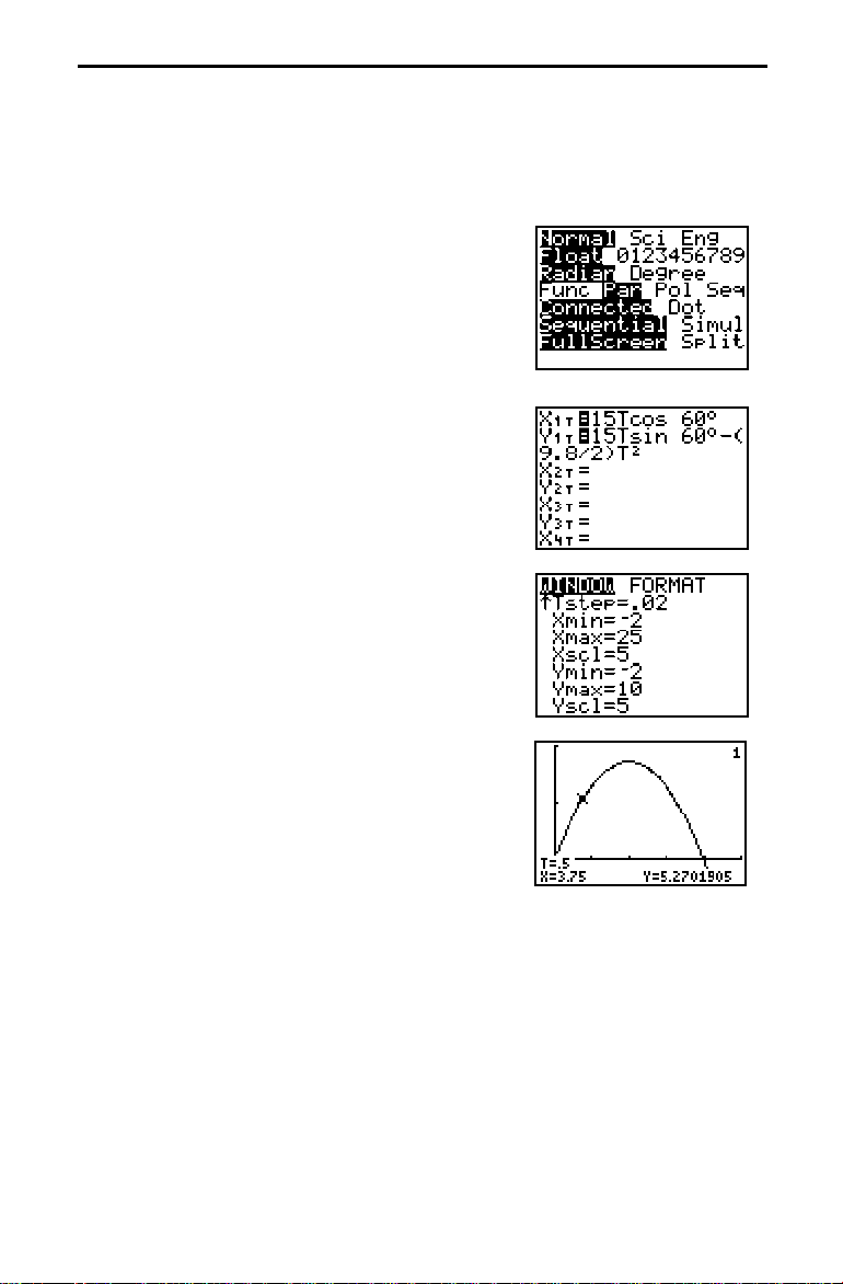
Getting Started: Path of a Ball
a
Getting Started is a fast-paced introduction. Read the chapter for details.
Graph the parametric equation that describes the position of a ball kicked at an
angle of 60¡ with an initial velocity of 15 meters per second. (Ignore air
resistance.) What is the maximum height? When does the ball strike the ground?
1. Press z. Press † † † ~
MODE
.
Par
Í
to select
For initial velocity v0 and angle q, the horizontal
component of the position of the ball as a
function of time is X(t)=tv
component is Y(t)=tv
constant g is 9.8 m/sec
2. Press o. Press 15
(to select ¡)
„ ™
Í
to define the X portion of the
parametric equation in terms of
9.8
¥ 2 ¤
„ ˜
60 y
„ ¡ Í
3. Press 15
¹ £
cosq. The vertical
0
sinq–(gà2)t2. The gravity
0
2
.
ã
.
T
ä
(to select ¡)
1
ANGLE
60 y
ã
ANGLE
to define the
portion.
4. Press
p
then enter the
. Press † to move to
WINDOW
variables appropriate
Tmin
for this problem.
Tmin=0 Xmin=-2 Ymin=-2
Tmax=3 Xmax=25 Ymax=10
Tstep=.02 Xscl=5 Yscl=5
5. Press
r
to graph the position of the ball as
function of time.
Tracing begins at
. As you press ~ to trace
Tmin
the curve, the cursor follows the path of the ball
over time. The values for
(distance),
X
Y
(height), and T (time) are displayed at the
bottom of the screen.
and
ä
1
Y
4-2 Parametric Graphing
Page 89

Defining and Displaying a Parametric Graph
Parametric equations consist of an X component and a Y component, each
expressed in terms of the same independent variable T. They are often used to
graph equations over time. Up to six pairs of parametric equations can be defined
and graphed at a time.
Defining a Parametric Graph
The steps for defining a parametric graph are the same as those for defining
a function graph. Differences are noted below.
Setting Parametric Graph Modes
Press z to display the
you must select
before you enter
Par
components of parametric equations. Also, you usually should select
Connected
Displaying Parametric Equations
After selecting
to obtain a more meaningful
Par
MODE
screen.
settings. To graph parametric equations,
MODE
WINDOW
variables or enter the
graph.
Par
, press o to display the parametric Y= edit
On this screen, you display and enter both X and Y components. TI.82 has
six equations, each defined in terms of
Defining Parametric Equations
Follow the same procedures as for
.
T
graphing to enter the two
Func
components that define a new parametric equation.
¦
You must define both the X and Y components in a pair.
¦
The independent variable in each component is T. You may press
ã
ä
T
rather than pressing
defines the independent variable as T.)
MODE
ƒ
, to enter the parametric variable
Parametric Graphing 4-3
. (
T
„
Par
,
Page 90

Selecting Parametric Equations
Only the selected parametric equations are graphed. The = sign on both
components of selected equations is highlighted. You may select any or all
of the equations on the parametric
edit screen.
Y=
To change the selection status of a parametric equation, press | to move
the cursor onto the
The status on both the
sign on either the X or Y component and press
=
and Y components is changed.
X
Note: When you enter both components of an equation or edit either
component, that equation is selected automatically.
Setting WINDOW Variables
p
Press
WINDOW
standard values in
Tmin=0
Tmax=6.2831853
Tstep=.1308996
Xmin=-10
Xmax=10
Xscl=1
Ymin=-10
Ymax=10
Yscl=1
to display the current
variables define the viewing
MODE
.
Radian
Smallest T value to evaluate
…
Largest T value to evaluate (2p)
…
value increment (pà24)
T
Smallest X value to be displayed
Largest X value to be displayed
Spacing between X tick marks
Smallest Y value to be displayed
Largest Y value to be displayed
Spacing between Y tick marks
WINDOW
WINDOW
variable values. The
. The values shown are the
Í
.
You may want to change the T
sufficient points are plotted.
4-4 Parametric Graphing
WINDOW
variable values to ensure that
Page 91

Setting the WINDOW FORMAT
p ~
Press
to display the current
formats are shared with the other graphing modes.
Displaying a Graph
When you press
It evaluates both the
to
The
in intervals of
Tmax
WINDOW
s
, the TI.82 plots the selected parametric equations.
and the Y component for each value of T (from
X
) and then plots each point defined by X and Y.
Tstep
variables define the viewing
As a graph is plotted, the TI.82 updates X, Y, and T.
Smart Graph applies to parametric graphs.
WINDOW Variables and Y-VARS Menus
From the Home screen, you can:
¦
Access functions by using the name of the component of the equation
as a variable.
¦
Select or deselect parametric equations from a program.
¦
Store parametric equations.
¦
Store values directly to
WINDOW
WINDOW FORMAT
WINDOW
variables.
settings. The
Tmin
.
Parametric Graphing 4-5
Page 92

Exploring a Parametric Graph
As in Function graphing, three tools are available for exploring a graph: using the
free-moving cursor, tracing an equation, and zooming.
Free-Moving Cursor
The free-moving cursor works in
TRACE
graphing. In
is
FORMAT
and
TRACE
CoordOn
q
are updated, and R and q are displayed.)
lets you move the cursor along the equation one
RectGC
FORMAT
) the values of X and Y. (In
When you begin a trace, the cursor is on the first selected equation at
The number of the equation shows in the upper right of the display.
In
the values of
updated, and
calculated from
RectGC
FORMAT, TRACE
, and T. (In
X, Y
, q, and T are displayed.) The X and Y (or R and q) values are
R
.
T
updates and displays (if
If the cursor moves off the top or bottom of the screen, the coordinate
values at the bottom of the screen continue to change appropriately.
y |
and y ~ move the
cursor remains in the same location if you leave
TRACE
TRACE
if Smart Graph has not caused the graph to be replotted.
QuickZoom is available in
Par
graphing just as it does in
Par
Func
, moving the cursor updates and displays (if
PolarGC
FORMAT
PolarGC
FORMAT
Tstep
FORMAT
, X, Y, R, q and T are
, X, Y, R,
at a time.
is
CoordOn
cursor five plotted points at a time. The
and return,
TRACE
graphing, but panning is not.
Tmin
.
)
ZOOM
operations work in
ZOOM
the
X (Xmin, Xmax
, and
variables are affected. T
not affected, except when you select
= pà24).
CALC
Tstep
, and
ZTmax
operations work in
CALC
ZOOM MEMORY
.
ZTstep
operations available in
4-6 Parametric Graphing
graphing as they do in
Par
) and Y (
Xscl
WINDOW
Ymin, Ymax
variables (
ZStandard (Tmin
variables in
graphing as they do in
Par
graphing are
Par
Func
, and
Yscl
Tmin, Tmax
= 0,
graphing include
Par
Func
value, dy/dx, dy/dt
graphing. Only
)
WINDOW
, and
Tmax
graphing.
, and
Tstep
= 2p, and
ZTmin
dx/dt
) are
CALC
,
.
Page 93

Chapter 5: Polar Graphing
This chapter describes how to graph polar equations on the TI.82. Before doing
polar graphing, you should be familiar with Chapter 3, Function Graphing.
Chapter Contents
Getting Started: Polar Rose
Defining and Displaying a Polar Graph
Exploring a Polar Graph
.....................
.............
.......................
5-2
5
5
-
3
-
6
Polar Graphing 5-1
Page 94
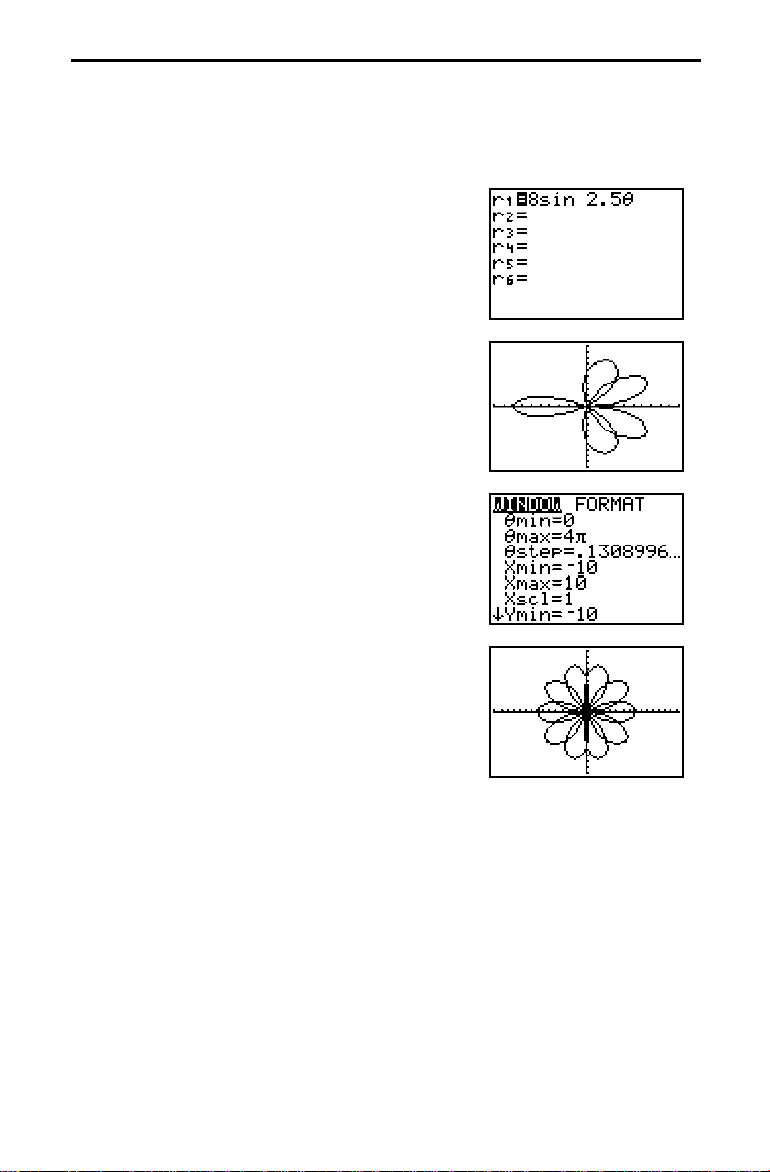
Getting Started: Polar Rose
Getting Started is a fast-paced introduction. Read the chapter for details.
The polar equation A sin Bq graphs a rose. Graph the rose for A=8 and B=2.5, and
then explore the appearance of the rose for other values of A and B.
1. Press z. Press † † † ~ ~
Pol
. Choose the initial settings for the
MODE
Í
other modes (the choice at the beginning of
each line).
2. Press o to display the polar
Press
3. Press
˜
8
q
„ Í
2.5
6 to select
ZStandard
equation in the standard viewing
edit screen.
Y=
to define
to graph the
WINDOW
Notice that the graph shows only five petals of
the rose and that the rose does not appear
symmetrical. This is because the standard
WINDOW
defines the
pixels) as square and sets
4. Press
5. Press
p
Press † †
q
.
max
q
to display the
y
4
5 to select
WINDOW
p
ä
ã
to increase the value of
q
max=2
WINDOW
ZSquare
(rather than the
p
.
and plot the
graph.
6. Continue, changing
and B to other values.
A
to select
1
.
r
.
settings.
5-2 Polar Graphing
Page 95

Defining and Displaying a Polar Graph
Polar equations are defined in terms of the independent variable q. Up to six polar
equations can be defined and graphed at a time.
Defining a Polar Graph
The steps for defining a polar graph are the same as those for defining a
function graph. Differences are noted below.
Setting Polar Graph Modes
Press z to display the
must select
before you enter
Pol
equation. Also, you usually should select
meaningful
Displaying Polar Equations
After selecting
Pol
graph.
Pol
MODE
On this screen, you display and enter polar equations. The TI.82 has six
equations, each defined in terms of
settings. To graph polar equations, you
MODE
WINDOW
variables or enter a polar
Connected
to obtain a more
, press o to display the polar Y= edit screen.
q
.
Defining Polar Equations
Follow the same procedures as for
graphing to define a new polar
Func
equation. The independent variable in a polar equation is
q
ã
„
, rather than pressing
(
Pol
Selecting Polar Equations
defines the independent variable as q.)
MODE
ƒ
ä
, to enter the polar variable
Only the selected polar equations are graphed. The = sign on selected
equations is highlighted. You may select any or all of the equations on the
polar
edit screen.
Y=
To change the selection status of a polar equation, press | to move the
cursor onto the
sign and press
=
Í
.
Note: When you edit an equation, that equation is selected automatically.
Polar Graphing 5-3
q
. You may press
q
.
Page 96

Setting WINDOW Variables
p
Press
WINDOW
to display the current
variables define the viewing
standard values in
q
min=0
q
max=6.2831853
q
step=.1308996
Xmin=-10
Xmax=10
Xscl=1
Ymin=-10
Ymax=10
Yscl=1
…
…
variable values. The
WINDOW
. The values shown are the
Radian
MODE
WINDOW
.
Smallest q value to be evaluated
Largest q value to evaluate (2p)
Increment between q values (pà24)
Smallest X value to be displayed
Largest X value to be displayed
Spacing between X tick marks
Smallest Y value to be displayed
Largest Y value to be displayed
Spacing between Y tick marks
You may want to change the q
WINDOW
sufficient points are plotted.
Setting the WINDOW FORMAT
p ~
Press
to display the current
formats are shared with the other graphing modes.
variable values to ensure that
WINDOW FORMAT
settings. The
5-4 Polar Graphing
Page 97

Displaying a Graph
When you press
evaluates
s
, the TI.82 plots the selected polar equations. It
for each value of q (from
R
q
min
to
q
in intervals of
max
and then plots each point.
As a graph is plotted, the TI.82 updates
X, Y, R
, and q.
Smart Graph applies to polar graphs.
Note that the free-moving cursor displays X and Y coordinate values if the
WINDOW FORMAT
PolarGC
WINDOW Variables and Y-VARS Menus
WINDOW FORMAT
setting is the default
.
. To see R and q, select
RectGC
From the Home screen, you can:
¦
Access functions by using the name of the equation as a variable.
¦
Select or deselect polar equations from a program.
¦
Store polar equations.
¦
Store values directly to
WINDOW
variables.
q
step
)
Polar Graphing 5-5
Page 98

Exploring a Polar Graph
As in function graphing, three tools are available for exploring a graph: using the
free-moving cursor, tracing an equation, and zooming.
Free-Moving Cursor
The free-moving cursor works in
TRACE
graphing. In
is
FORMAT
and
TRACE
CoordOn
q
are updated, and R and q are displayed.)
lets you move the cursor along the equation one
RectGC
FORMAT
) the values of X and Y. (In
When you begin a trace, the cursor is on the first selected equation at
The number of the equation shows in the upper right of the display.
In
the values of
and
RectGC
FORMAT, TRACE
, and q. (In
X, Y
and q are displayed.)
R
updates and displays (if
PolarGC
If the cursor moves off the top or bottom of the screen, the coordinate
values at the bottom of the screen continue to change appropriately.
y |
and y ~ move the
cursor remains in the same location if you leave
TRACE
TRACE
if Smart Graph has not caused the graph to be replotted.
QuickZoom is available in
Pol
graphing just as it does in
Pol
Func
, moving the cursor updates and displays (if
FORMAT
PolarGC
FORMAT
q
step
FORMAT
, X, Y, R, and q are updated,
, X, Y, R,
at a time.
q
is
CoordOn
min
cursor five plotted points at a time. The
and return,
TRACE
graphing, but panning is not.
.
)
ZOOM
operations work in
ZOOM
the
X (Xmin, Xmax
, and
variables are affected. The q
are not affected, except when you select
q
and
Zqmin, Zqmax
CALC
CALC
CALC
= pà24). The
step
, and
Zqstep
operations work in
operations available in
5-6 Polar Graphing
graphing as they do in
Pol
) and Y (
Xscl
WINDOW
ZOOM MEMORY
Ymin, Ymax
variables (
.
graphing as they do in
Pol
graphing are
Pol
, and
q
min
ZStandard
variables in
value, dy/dx
graphing. Only
Func
)
Yscl
WINDOW
q
,
, and
max
q
(
= 0,
min
graphing include
Pol
graphing. The
Func
, and
q
max
dr/d
q
step
= 2p,
q
.
)
Page 99

Chapter 6: Sequence Graphing
This chapter describes how to graph sequences on the TI.82. Before doing
sequence graphing, you should be familiar with Chapter 3, Function Graphing.
Chapter Contents
Getting Started: Forest and Trees
Defining and Displaying a Sequence Graph
Exploring a Sequence Graph
...................
............
......................
6-2
6-3
6-6
Sequence Graphing 6-1
Page 100
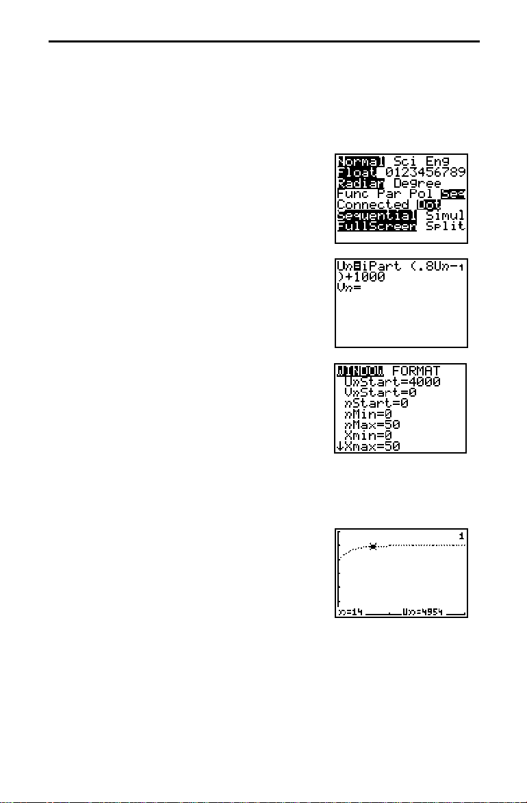
Getting Started: Forest and Trees
Getting Started is a fast-paced introduction. Read the chapter for details.
A small forest contains 4000 trees. The new forestry plan is that each year 20% of
the trees will be harvested and 1000 new trees will be planted. Will the forest
disappear? Does it stabilize at a certain number of trees? If so, what is that
number?
Í
Í
to select
to
1. Press z. Press † † † ~ ~ ~
select
Dot
Seq
MODE
MODE
.
. Press † ~
2. Press o. Each year the number of trees is 80
percent of what was there at the end of the prior
year. Press
~
(to select
2
iPart
, because
the company will not harvest part of a tree) £
ã
n-1
y
number of trees after each harvest. Press
1000
3. Press
Press
ä
U
(
function of ¬) ¤ to define the
2nd
to define the replacement trees.
p
. Press † to move to
Í
4000
to define the number of trees
UnStart
Ã
.
at the beginning of the program.
4. Press † † †
50
Í
to set
n
Max=50
to plot
the size of the forest over 50 years.
5. Set the other
Xmin=0 Ymin=0
Xmax=50 Ymax=6000
Xscl=10 Yscl=1000
6. Press
WINDOW
r
. Tracing begins at
variables:
n
Min
(before the
forestry program began). Press ~ to trace the
values year-by-year. The values for
(trees) are displayed at the bottom of the
U
n
(year) and
n
screen. How many years does it take to stabilize
the size of the forest?
.8
6-2 Sequence Graphing
 Loading...