

TI-83 Plus CellSheet™
TI
Application
Getting Started
Start here
How To…
Enter data Edit data
Create charts Import and export data
Examples
Scatter chart Bar chart
Pie chart Linear regression
Gravity Simple interest
Fibonacci numbers
Slope of secant and tangent lines
More Infor m a t ion
Customer Support Error Recovery
2/28/02 © 2001 Texas Instruments

Important Information
Texas Instruments makes no warranty, either expressed or
implied, including but not limited to any implied warranties of
merchantability and fitness for a particular purpose, regarding
any programs or book materials and makes such materials
available solely on an “as-is” basis.
In no event shall Texas Instruments be liable to anyone for
special, collateral, incidental, or consequential damages in
connection with or arising out of the purchase or use of these
materials, and the sole and exclusive liability of Texas
Instruments, regardless of the form of action, shall not exceed
the purchase price of this item or material. Moreover, Texas
Instruments shall not be liable for any claim of any kind
whatsoever against the use of these materials by any other
party.
Graphing product applications (Apps) are licensed. See the
terms of the license agreement
for this product.
Windows, NT, Apple, and Mac are trademarks of their respective owners.
TI-83 Plus CellSheet™ Application Page 2

What is the CellSheet Application?
The CellSheetËapplication combines spreadsheet functionality
with the power of the TI83 Plus. The CellSheet application can
be useful in classes other than math, such as social studies,
business, and science.
Cells can contain:
Integers
•
Real numbers
•
Formulas
•
Variables
•
Text and numeric strings
•
Functions
•
Each spreadsheet contains 999 rows and 26 columns. The
amount of data you can enter is limited only by the available
RAM on your TI83 Plus.
TI-83 Plus CellSheet™ Application Page 3

What You Need
To install and run the application, you need:
A TI-83 Plus calculator with version 1.13 or higher of the
•
operating system software to optimize the performance of your
calculator and the application
-
To check the operating system version, press
and then select
About
below the product name.
-
You can download a free copy of the latest operating
system software from education.ti.com/softwareupdates
Follow the link to Operating Systems.
.
. The version number is displayed
\ /
,
.
A computer with Windows
•
Apple
A TI-GRAPH LINK™ computer-to-calculator cable. If you do
•
®
Mac®OS 7.0 or later installed.
®
95/98/2000, Windows NT®, or
not have this cable, call your distributor, or order the cable
from TI's online store
TI Connect™ or TI-GRAPH LINK software that is compatible
•
.
with the TI83 Plus. You can download a free copy of
TI Connect or TI-GRAPH LINK software from
education.ti.com/softwareupdates
. Follow the link to
Connectivity Software.
TI-83 Plus CellSheet™ Application Page 4

Where to Find Installation Instructions
Detailed instructions on installing this and other applications are
available at education.ti.com/guides
installation instructions.
. Follow the link to Flash
Getting Help
This application has a built-in help screen that gives you basic
information about using the application. The help screen is
automatically displayed when you start the application.
To display the help screen from the main spreadsheet
•
screen, select
To exit the help screen and return to the main spreadsheet
•
screen, press any key.
The instructions in this guidebook are only for this application. If
you need help using the TI83 Plus, refer to its comprehensive
guidebook at education.ti.com/guides
Menu
(press
V
), and then select
.
Help
.
TI-83 Plus CellSheet™ Application Page 5

Quick Reference Guide
Note
By default, the help screen is displayed when you start the
CellSheet application. However, you can turn off this feature.
Starting the Application
1. Press
, and then select
n
CelSheet
screen is displayed.
2. Press any key to continue. The CellSheet™ help screen is
displayed.
3. Press any key to continue.
Quitting the Application
From the main spreadsheet screen, press
•
From the
•
CELLSHEET MENU
, select
. The information
\
Quit CellSheet
.
.
TI-83 Plus CellSheet™ Application Page 6

Deleting the Application from Your Calculator
Task
Instructions
Enter a value in a
cell
Enter the value, and then press
¯
.
Enter text or a
numeric string in a
cell
1. Press
e
É
.
2. Enter the text.
3. Press
¸
.
1. Press
2. Select
3. Select
\ /
Mem Mgmt/Del
.
Apps
4. Move the cursor to
5. Press
6. Select
. A confirmation message is displayed.
^
to delete the application.
Yes
Completing Tasks
to display the MEMORY menu.
.
.
CelSheet
TI-83 Plus CellSheet™ Application Page 7

Task
Instructions
Create a formula
1. Press
¡
or ¥.
2. Enter a formula.
3. Press
¯
.
Use a variable in a
spreadsheet
1. From the TI83 Plus home screen, store a value
to a variable (for example, 5
§ Ù
).
2. Start the CellSheet™ application, and open the
spreadsheet file.
3. Move the cursor to a cell and type the variable
(such as X). Do not surround the variable with
quotation marks.
4. Press
¸
. The variable's value appears in the
cell.
Tip
: You can also use variables in formulas
(e.g., =
X
h
A5) or in cell calculations (e.g., log(X)).
If you change the value of a variable, you must
manually recalculate the spreadsheet.
Navigate rapidly in
a spreadsheet
•
Press
e h
to page down by 6 rows.
•
Press
e `
to page up by 6 rows.
•
To jump to a specific cell, select
Menu
, select
Edit > Go To Cell
, and then enter the cell
address.
Note:
Press
e
before typing alpha characters.
TI-83 Plus CellSheet™ Application Page 8

Task
Instructions
Switch between the
spreadsheet and a
chart or graph
1. Select
Menu
, select
Charts
, and then select the
chart you want to display.
2. To return to the spreadsheet, press
\
.
Select a range of
cells
1. Move the cursor to the starting cell, and then
press
R
.
2. Use _, `, a, and has needed to select the
range.
Tip:
For a large range, it might be faster to select
Menu
, select
Edit > Select Range
, and then specify
the range (for example, A6:A105).
Insert a row
1. Press _as needed to select the row.
2. Press
2 /
to insert a row above the selected
row.
Insert a column
1. Press `or
e `
as needed to select the
column.
2. Press
2 /
to insert a column to the left of the
selected column.
TI-83 Plus CellSheet™ Application Page 9

Task
Instructions
Delete a row or
column
1. Move the cursor to the row header or column
header to select the row or column.
2. Press
^
.
The columns to the right of the deleted column
shift left.
The rows below a deleted row shift up.
Clear data from a
cell, cell range, row,
or column
1. Select one or more cells, a row, or a column.
2. Press
M
.
TI-83 Plus CellSheet™ Application Page 10

Task
Instructions
Cut, copy, and
paste
To cut or copy a cell:
1. Move the cursor to the cell.
2. Press
S
to cut the cell.
—or—
Press
T
to copy the cell.
To cut or copy a range of cells:
1. Move the cursor to the first cell in the range.
2. Press R.
3. Move the cursor to the last cell in the range.
4. Select
Cut
(press
S
) to cut the cell range.
—or—
Select
Copy
(press
T
) to copy the cell range.
To paste:
1. Cut or copy one or more cells.
2. Move the cursor to the new cell (or the first cell of
a new cell range).
3.
Select
Paste
(press
U
).
TI-83 Plus CellSheet™ Application Page 11

Task
Instructions
Grab cell reference
1. While entering or editing a formula, place the
cursor on the edit line where you want to enter a
cell reference.
2. Press
n
.
3. Use the arrow keys to move the cursor to the cell
that contains the formula or value that you want
to copy.
4. Press
¯
. The address of the cell you
referenced appears on the edit line (where you
placed the cursor in step 1) and is now part of the
current formula.
Grab range
reference
1. While entering or editing a formula, place the
cursor on the edit line where you want to enter a
range reference.
2. Press
n
.
3. Use the arrow keys to move the cursor to the first
cell in the range that you want to copy.
4. Press R, and then move the cursor to the last
cell in the range that you want to copy.
5. Press
¯
. The cell range that you referenced
appears on the edit line (where you placed the
cursor in step 1) and is now part of the current
formula.
TI-83 Plus CellSheet™ Application Page 12

CellSheet Main Menu
Menu Item
Description
1: Open
Opens an existing spreadsheet file.
2: Save As
Saves the current spreadsheet with a different name.
3: New
Creates a new spreadsheet and lets you enter a unique
name.
4: Delete
Deletes a spreadsheet. You cannot delete the currently
open spreadsheet.
To display the
•
To display a help screen for common tasks, select
•
the
CELLSHEET MENU
To exit the application, select
•
CELLSHEET MENU
•
Press
-
-
s
Return to the main menu from a submenu
Return to the spreadsheet from the main menu
CELLSHEET MENU,
.
.
or
\
to
select
Quit CellSheet
File Menu
Menu
(press
V
Help
from the
).
from
TI-83 Plus CellSheet™ Application Page 13

Menu Item
Description
5: Format
Lets you set up formatting options such as automatic
recalculation, cursor movement, help screen display, and
edit line display.
6: Recalc
Recalculates the spreadsheet (only needed when the
autocalculation feature in the Format menu is turned off)
Menu Item
Description
1: Go To Cell
Moves the cursor to a specific cell.
2: Undelete Cell
Retrieves the contents of the cell that you just deleted or
cleared.
3: Clear Sheet
Deletes all data from the current spreadsheet.
4: Select Range
Selects a range of cells.
5: Cut
Cuts the contents and formulas from the currently selected
cell or range of cells and places them on the clipboard.
(Shortcut key:
S
)
6: Copy
Copies the contents and formulas from the currently
selected cell or range of cells and places them on the
clipboard. (Shortcut key:
T
)
7: Paste
Pastes the contents and formulas that were just cut or
copied to the clipboard into the current cell. (Shortcut key:
U
)
Edit Menu
TI-83 Plus CellSheet™ Application Page 14

Options Menu
Menu Item
Description
1: Statistics
Calculates 1-variable statistics, 2-variable statistics, or
linear regression for the currently selected cell range.
2: Fill Range
Fills a range of cells with a formula, number, or text.
3: Sequence
Fills a range of cells with a sequence of numbers.
4: Import/Export
Imports lists or matrices, or variables; exports lists,
matrices, or variables.
5: Sort
Sorts a range of cells in ascending or descending order.
6: Col Decimal
Sets the decimal mode display for a column. The calculator
decimal mode display (accessed by pressing
]
) does
not affect the CellSheet™ application.
TI-83 Plus CellSheet™ Application Page 15

Charts Menu
Menu Item
Description
1: Scatter
Displays a scatter chart for a range of cells.
2: Scatter Window
Displays the parameters for the viewing window for the
scatter chart so that you can change the values.
3: Line
Displays a line chart for a range of cells.
4: Line Window
Displays the parameters for the viewing window for the line
chart so that you can change the values.
5: Bar
Displays a bar chart for a range of cells.
6: Bar Window
Displays the parameters for the viewing window for the bar
chart so that you can change the values.
7: Pie
Displays a pie chart for a range of cells.
TI-83 Plus CellSheet™ Application Page 16

Starting and Quitting the Application
Note
By default, the help screen is displayed when you start the
CellSheet™ application. However, you can turn off this feature.
Starting the Application
1. Press
n
to display the list of applications on your
calculator.
2. Select
CelSheet
. The information screen is displayed.
3. Press any key to continue. The help screen is displayed.
4. Press any key to continue. A blank spreadsheet (or the last
spreadsheet that you opened) displays, and cell A1 is
selected.
The first four characters of the spreadsheet's name appear
in the upper left corner of the spreadsheet. You can press
_ `
to highlight the name cell and view the full name on the
edit line.
TI-83 Plus CellSheet™ Application Page 17

Quitting the Application
•
Press
\
from the main spreadsheet screen.
—or—
Select
•
screen, and then select
Menu
(press
V
) from the main spreadsheet
Quit CellSheet
.
Getting Started
Work through the following example to get acquainted with the
main features of the CellSheet™ application.
Example–
purchase a $1500 item. QuickCash charges 1.5 percent
interest that is compounded monthly. The required minimum
monthly payment is 3 percent of the balance. Assuming that
Margaret makes the minimum monthly payment, how much
interest and principal will she have paid in six months?
Start the CellSheet application.
Margaret used her QuickCash credit card to
1. Press
n
to display the list of applications on your
calculator.
TI-83 Plus CellSheet™ Application Page 18

2. Select
Note
If the last spreadsheet that you opened is displayed, create a
new spreadsheet file. To do this, select
Menu
(press
V
),
select
File> New
, enter a name for the spreadsheet, and then
press
¯
two times.
Tip
•
To indicate that an entry is a text string, press
e
["].
•
To turn on alpha-lock mode, press
\
.
•
To complete an entry, press
¯
.
CelSheet
. The information screen is displayed.
3. Press any key to continue. The help screen is displayed.
4. Press any key to continue. A blank spreadsheet (or the last
spreadsheet that you opened) is displayed.
Enter these column headings:
= principal
P
= interest accrued
I
= minimum monthly payment
PMT
1. With the cursor in cell A1, enter the principal column
heading,
(
\
P
["]
¯
P
).
2. Move the cursor to cell B1, and enter the interest accrued
column heading,
TI-83 Plus CellSheet™ Application Page 19
(
\
I
["]
¯
I
).

3. Move the cursor to cell C1, and enter the minimum monthly
Note
To indicate that an entry is a formula, press
¡
to place an
equal sign on the edit line.
payment column heading,
Your spreadsheet should look like this:
Enter the initial data for the spreadsheet in cells A2, B2, and
C2.
P = 1500
I = P
4
.015
PMT = P 4.03
PMT
(
\
["]
PMT
¯
).
1. Move the cursor to cell A2, and enter
1500
. (
1500
¯
)
2. Move the cursor to cell B2, and then enter the formula
A2
44
=
TI-83 Plus CellSheet™ Application Page 20
.015
. (
¡ e
A2
015
¯
)

3. Move the cursor to cell C2, and then enter the formula
= A2
(
44
¡ e
.03
A2
03
¯
).
Your spreadsheet should look like this:
At the beginning of each month, the new principal, P
calculated using the following formula: P
where P
, PMT1, and I1all pertain to the previous month. The
1
= P1– (PMT1– I1),
2
, is
2
interest and minimum monthly payment are calculated exactly
as they were for the first month. Enter the remaining
spreadsheet formulas to find the solution to the problem.
1. Move the cursor to cell A3, and then enter the formula
= A2 – (C2 – B2)
¯
).
(
¡ e
e
A2
e
C2
B2
2. To copy the formulas from B2:C2 to B3:C3, place the cursor
in cell B2, and press Rto begin the range selection.
TI-83 Plus CellSheet™ Application Page 21

3. Press ato move the cursor to C2, and then select
(press
T
) to copy the formula from this range of cells.
Copy
4. Move the cursor to cell B3, and then select
U
5. Press
TI-83 Plus CellSheet™ Application Page 22
) to paste the formula from this range of cells.
\
to exit the copy/paste mode.
Paste
(press

Enter the data for the remaining four months by copying the
Tip
•
To copy and paste a range of cells, press R, select the range,
select
Copy
(press
T
), move the cursor to the new
location, and then select
Paste
(press
U
).
•
To copy a single cell, press
T
, move the cursor to the new
location, and then select
Paste
.
formulas from A3:C3 to rows 4 through 7.
1. With the cursor in cell A3, copy the formulas from A3:C3 (
Copy
a a
2. Move the cursor to cell A4, and then select
U
3. Move the cursor to cell A5, and then select
).
) to paste the formulas into A4:C4.
Paste
Paste
(press
to paste the
R
formulas into A5:C5.
4. Paste the formulas to A6:C6 and A7:C7.
5. Press
\
to exit copy/paste mode.
6. Move the cursor to cell A7, copy the formula, and paste it in
cell A8 (
T h
\
). This amount, $1370, is the
Paste
remaining principal to be paid after six payments have been
made.
TI-83 Plus CellSheet™ Application Page 23

Your spreadsheet should look like this:
Using the following formulas, calculate how much interest and
principal Margaret will have paid after six months.
The total principal paid is 1500 – P
The total interest paid is the sum of I
The total of the payments made is the sum of PMT
PMT
.
6
.
7
through I6.
1
through
1
1. Move the cursor to cell A9, and then enter the formula
=1500 – A8
¡
1500
e
(
2. Move the cursor to cell B9, and then press
3. Press
sum(
4. Press
5. Press
TI-83 Plus CellSheet™ Application Page 24
V
.
n
R
to display a list of functions, and then select
, and then move the cursor to cell B2.
to begin range selection.
A8
¯
).
¡
.

6. Move the cursor to cell B7, and then press
Tip
You could also directly enter the formula by pressing
¡
V1eB2e
[:]
eB7 ¯
.
You can see that after 6
months, Margaret will have
paid $260.08, which included
$130.04 in interest and
$130.04 in principal.
¯
.
7. Press to complete the formula, and then press
8. Move the cursor to cell B9, copy the formula, and then paste
it in cell C9 (
T a
Paste
Your spreadsheet should look like this:
Save the spreadsheet with the name
Each spreadsheet is automatically saved in RAM as you work on
it. Default names, beginning with S01, are used to name the
spreadsheets before you save your file with a unique name.
\
).
INTEREST
.
¯
.
1. Select
TI-83 Plus CellSheet™ Application Page 25
menus.
Menu
(press
V
) to display the CellSheet™

2. Select
Note
•
The spreadsheet name must begin with a letter, but can
contain both letters and numbers.
•
The spreadsheet name can have up to 8 characters.
cursor is at the
File > Save As
New
. The old name is displayed, and the
prompt. Alpha-lock is turned on.
3. At the
prompt, type
New
INTEREST
spreadsheet, and then press
4. Press
¯
again to accept the name and return to the
spreadsheet screen. The first few letters of the new
spreadsheet name are displayed in the upper left corner of
the screen.
Quit the application.
From the main spreadsheet screen, press
as the name for this
¯
.
\
.
TI-83 Plus CellSheet™ Application Page 26

Creating, Saving, and Opening Files
Tip
The spreadsheet name
•
can contain numbers and letters, but must begin with a letter
•
can contain up to 8 characters
TICSFILE is a reserved name used by the CellSheet™
application.
Creating a File
To create a new, blank spreadsheet:
1. Select
2. Select
Menu
>
File
(press
.
New
V
) to display the
3. Enter a name for the new spreadsheet, and then press
¯
two times. A new, blank spreadsheet is displayed.
CELLSHEET MENU
.
TI-83 Plus CellSheet™ Application Page 27

Saving a File
Tip
The spreadsheet name
•
can contain numbers and letters, but must begin with a letter
•
can contain up to 8 characters
TICSFILE is a reserved name used by the CellSheet™
application.
The spreadsheet is automatically saved in RAM as you work.
You do not have to manually save your work. However, you can
save the current spreadsheet with a new file name.
To save a file with a new name:
1. Select
2. Select
Menu
>
File
(press
Save As
V
.
).
3. Enter a name for the new spreadsheet, and then press
¯
two times. The spreadsheet is displayed, and the first
four characters of the new name are displayed in the top left
cell.
TI-83 Plus CellSheet™ Application Page 28

Opening a File
Tip
•
Only one spreadsheet can be open at a time.
•
Names of archived spreadsheets do not appear in the list. You
must unarchive a spreadsheet before you can open it.
1. Select
2. Select
(press
Menu
, and then select
File
V
).
Open
names is displayed.
3. Move the cursor to the spreadsheet name that you want to
open, and then press
¯
.
Managing Files
Copying a File
To copy a spreadsheet file, save the file with a new name
Deleting a File
1. Select
2. Select
Menu
>
File
(press
Delete
V
.
).
. A list of spreadsheet file
.
TI-83 Plus CellSheet™ Application Page 29

3. Move the cursor to the spreadsheet file name that you want
Note
You cannot delete the spreadsheet that is currently open.
Tip
•
If you need to free RAM on your TI83 Plus, you can save a
copy of a spreadsheet on your computer using TIConnect™ or
TI-GRAPH LINK™ software before you delete it.
•
You can also delete a spreadsheet using the memory
management menu from the home screen (
\ /
,
Mem Mgmt/Del> AppVars
{spreadsheet name}
^
Yes
).
to delete, and then press
¯
.
4. Select
Yes
. The spreadsheet file is deleted.
Renaming a File
To rename a file, save the file with a new name
the old spreadsheet.
, and then delete
TI-83 Plus CellSheet™ Application Page 30
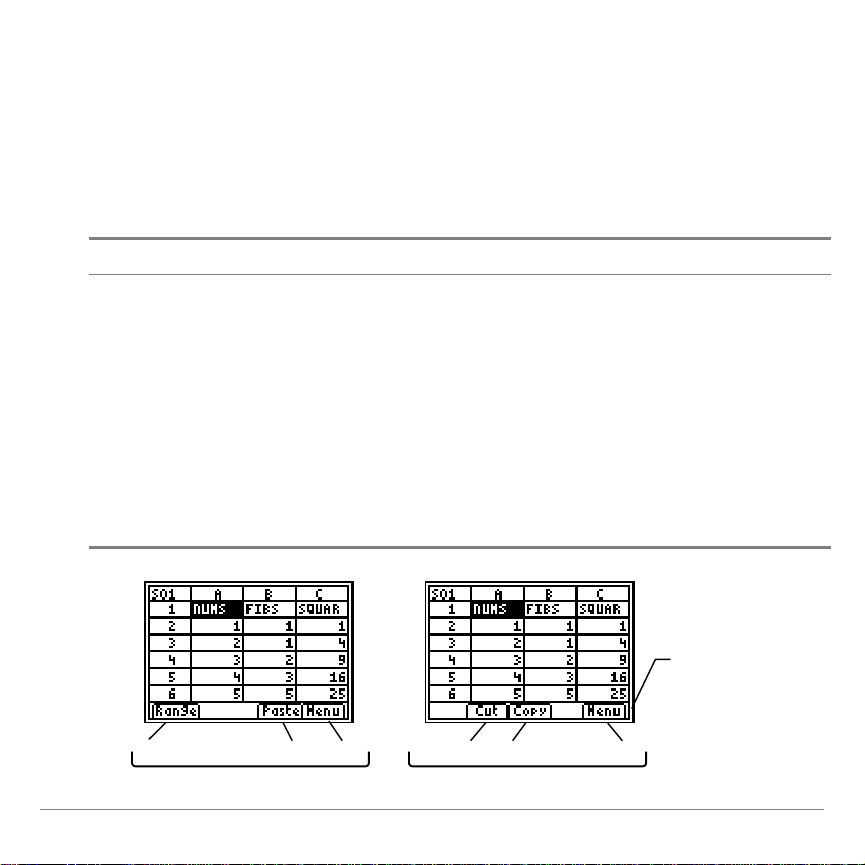
Using CellSheet Commands
Option
Description
Range (press R)
Turns on range selection mode
Cut (press
S
)
Allows the contents of the cell or range of cells to
be moved to a new location using the
Paste
tool
Copy (press
T
)
Allows the contents of the cell or range of cells to
be copied to a new location using the
Paste
tool
Paste (press
U
)
Pastes the contents of the cell or range of cells
selected with
Cut
or
Copy
to the cursor location
Menu (press
V
)
Displays the CellSheet™ main menu
R S T U V
R S T U V
Press a graphing
key to select a
command.
The CellSheet™ application displays commands at the bottom of
the screen at various times to help you complete specific tasks.
To select a command, press the graphing key directly below the
command.
TI-83 Plus CellSheet™ Application Page 31

Working with Spreadsheets
Tip
Press
e
before entering the column letter of the cell address
at the Cell prompt.
Navigating in the Spreadsheet
Use the arrow keys to move from one cell to another.
•
•
•
•
Press
Press
e h
e `
To jump to a specific cell, select
, enter the cell address, and then press
Cell
to move the cursor down 6 rows.
to move the cursor up 6 rows.
Menu
, select
¯
Edit > Go To
two times.
TI-83 Plus CellSheet™ Application Page 32

Changing the Default Values for Individual Spreadsheets
Menu Item
Description
Default Setting
AutoCalc
Automatically recalculates the entire
spreadsheet as you work; does not
automatically recalculate the spreadsheet
upon opening the file.
Note
: When AutoCalc is set to N, cells with
new formulas that you create will display
the value 0 until you manually recalculate
the spreadsheet.
Y (yes)
Cursor Mvmt
Controls the direction that the cursor
moves after you press
¯
on the edit
line.
(down)
Init Help
Controls whether the help screen is
displayed when you start the application.
Y (yes)
Show
Controls what information is displayed on
the edit line – formulas or resultant values.
FMLA (formula)
Select
Menu
, select
File
>
following default settings. The changes only apply to the current
spreadsheet.
Format
, and then change any of the
TI-83 Plus CellSheet™ Application Page 33

Entering Spreadsheet Data
Caution
As you enter data into a large spreadsheet, each entry may
require a few seconds of processing time, particularly if the
AutoCalc feature is on. The CellSheet™ application does not
recognize keystrokes that are made during the processing time.
A numeric value, text string, or formula that is entered into a
•
single cell can contain a maximum of 40 characters.
Numeric values are right-justified in the cell; text is left-
•
justified.
The number of characters that are displayed is limited by the
•
column decimal format
contents of the adjacent cell(s) for text. The edit line displays
the entire contents of the cell.
The displayed value of the cell is rounded to the number of
•
decimal places specified by the column decimal format
However, the actual value of the cell is used in calculations.
Cells that contain text are treated as if they contained the
•
value 0 when they are referenced in math operations,
statistics, or charts.
Cells that contain text are ignored when they are referenced
•
in cell ranges that are used in formulas.
for numeric values, and by the
.
TI-83 Plus CellSheet™ Application Page 34

Entering Numbers and Text
Note
The CellSheet™ application does not support complex numbers.
To enter a numeric value in a cell, type the number, and then
•
press
¯
. Values can be entered in normal, scientific, or
engineering notation. The way the values are displayed is
determined by the calculator's notation mode. You can
change the notation mode from the calculator's home screen
by pressing
, and then selecting
]
Normal, Sci
or
Eng
.
To enter text in a cell, press
•
e
["] (or
\
["]), and
then enter the text. Any character string that is preceded by
quotation marks is treated as text. Dates and times must be
entered as text.
To enter the last entry from the home screen, press
•
\ >
home screen by pressing
TI-83 Plus CellSheet™ Application Page 35
. You can cycle through the last few entries on the
\ >
multiple times.

Entering a Formula
Cell reference
Numeric constant
Spreadsheet function
Range reference
A formula is an equation that performs operations on
spreadsheet data. Formulas can:
Perform mathematical operations, such as addition and
•
multiplication
Compare worksheet values
•
Refer to other cells in the same spreadsheet
•
When you use a formula, the formula and the evaluation of the
formula are both saved in the cell.
The following example adds 15 to the value in cell C4 and then
divides the result by the sum of the values in cells B4, B5, and
B6.
=(C4+15)/sum(B4:B6
TI-83 Plus CellSheet™ Application Page 36
)

To enter a formula, press
Note
•
If you do not precede a formula that contains a cell reference
with an equal sign, the application interprets the column
reference as a variable, which usually results in an error.
•
If a formula references a cell that is empty, ERROR or 0 is
displayed, depending on how the empty cell was used in the
formula.
Tip
•
The spreadsheet is not automatically recalculated upon
opening the spreadsheet file. You must manually recalculate
the spreadsheet if it contains references to lists, matrices, or
variables that have changed.
•
You may want to turn off the autocalc feature if your
spreadsheet is large. Large spreadsheets can take a minute
or more to recalculate.
¡
to place an equal sign on the edit
line, and then enter the formula.
If AutoCalc is turned on, the spreadsheet is automatically
recalculated as you enter data into or edit data in the
spreadsheet.
TI-83 Plus CellSheet™ Application Page 37

Entering an Absolute Cell Reference
Reference
Description
$A$1
Absolute column and absolute row
$A1
Absolute column and relative row
A$1
Relative column and absolute row
If you do not want a cell reference to be updated when you copy
or move a formula to a different cell, use an absolute reference.
(Relative references are updated when the cell is copied or cut
and moved to a new location.) You can enter the following types
of absolute references:
To enter an absolute cell reference, press
\ .
to place a
dollar sign on the edit line.
TI-83 Plus CellSheet™ Application Page 38

Entering a Function
Note
The ending parenthesis is required!
Equal sign required
because a cell range
is the argument for
the function
Function name
Argument
A function is a predefined formula that performs calculations by
using specific values in a particular order. The values are called
arguments. The arguments can be numbers, lists, cell names,
cell ranges, etc., depending on what the function requires. The
arguments are enclosed in parentheses, and a comma
separates each argument.
When a function uses a cell name or range as arguments, it
•
must be preceded by an equal sign; otherwise, no equal sign
is necessary.
=sum(A3:A25)
When the function is not preceded by an equal sign, only the
•
resulting value of the function is saved in the cell; the entire
function and its arguments are not saved.
TI-83 Plus CellSheet™ Application Page 39

If a function's argument is a list, a cell range is also a valid
•
argument.
If a function's argument is a value, a cell name is also a valid
•
argument.
You can use any function in the TI83 Plus catalog (
or in any menu, such as Math (
(
\
).
o
), List (
\
\ 1
), or Test
To enter a function:
1. Press
¡
to place the equal sign on the edit line, if
necessary.
2. Press
V
move the cursor to a function, and then press
to display a list of commonly used functions,
¯
to select
it.
—or—
Select a function from the calculator catalog or other menus,
such as Math, List, or Test.
3. Enter the argument(s) for the function, and then press
¯
)
.
TI-83 Plus CellSheet™ Application Page 40

Using the IF Function
Note
The CellSheet application does not support nested functions (a
function within a function).
Condition
statement
Command (ELSE)
statement
Command (THEN)
statement
In an IF function, the IF statement evaluates to true or false. The
THEN command is executed if the IF statement is true; the ELSE
command is executed if the IF statement is false.
When you need to use an IF function in a spreadsheet, press
¡ V
, and then select
If(
from the
FUNCTIONS
menu. The
IF function in the CellSheet ™ application is not the same as the
IF function in the TI83 Plus catalog. (The IF function in the
catalog is for programming.)
The condition statement (the IF statement) can contain cell
•
references, values, or variables.
The command statements (the THEN and ELSE statements)
•
can contain a values or expressions.
The operator symbols are available from the
•
)
=If(A3
dd
100,100,0)
TEST
menu (
TI-83 Plus CellSheet™ Application Page 41
\

Using Stored Variables
Note
You can use the Export Var option to store a value to a variable.
To use a stored variable in a cell or formula, enter the variable
name without using quotation marks. For example, enter
multiply the value stored in A by 5.
Copying Cells
When you copy a cell, the CellSheet™ application copies the
entire cell, including formulas and their resulting values. Relative
cell references are automatically updated when you paste the
cell(s) to a new location.
The following instructions show how to use the CellSheet
application's shortcut keys to copy and paste cells. You can also
use the commands from the
(select
, and then select
Menu
menu to copy and paste cells
EDIT
).
Edit
Copying a Single Cell
5ggA
to
1. Move the cursor to the cell that you want to copy.
2. Press
TI-83 Plus CellSheet™ Application Page 42
T
to copy the cell to the clipboard.

3. Move the cursor to the new cell where you want to paste the
Tip
You can paste the clipboard contents to a new cell multiple
times.
Tip
You can select an entire row or column by moving the cursor to
the row header or column header. The entire row or column is
highlighted when it is selected.
clipboard contents, and then select
Paste
(press
U
).
4. Press
\
to exit the copy/paste mode.
Copying a Single Cell to a Range of Cells
1. Move the cursor to the cell that you want to copy.
2. Press
T
to copy the cell to the clipboard.
3. Move the cursor to the first cell of the range where you want
to paste the clipboard contents.
4. Select
Range
the range, and then select
(press R), move the cursor to the last cell in
(press
Paste
U
).
TI-83 Plus CellSheet™ Application Page 43

Copying a Range of Cells
Tip
You can select an entire row or column by moving the cursor to
the row header or column header. The entire row or column is
highlighted when it is selected.
Tip
You can paste the clipboard contents to a new cell range multiple
times.
You can copy a range of cells using one of the following
methods.
Method 1:
1. Move the cursor to the first cell in the range.
2. Press R, and then move the cursor to the last cell in the
range.
3. Select
Copy
(press
T
) to copy the range to the clipboard.
4. Move the cursor to the first cell where you want to paste the
clipboard contents, and then select
Paste
(press
U
TI-83 Plus CellSheet™ Application Page 44
).

Method 2:
1. Select
, and then select
Menu
Edit
>
Select Range
.
2. Enter the range of cells (for example A1:A9) at the
prompt.
3. Press
¯
two times to select the range and return to the
spreadsheet. The last cell in the range is highlighted.
4. Select
to copy the range you selected, and then select
5. Press
\
, move the cursor to the first cell where you want
Copy
Paste
to exit the copy/paste mode.
Range
.
TI-83 Plus CellSheet™ Application Page 45

Editing Spreadsheet Data
Tip
If you have not yet pressed
¯
to change a cell's content, you
can press
\
to revert to the previous contents of a cell.
Editing Cell Contents
You can change a cell's contents by entering a new text string,
value, or formula in place of the existing one.
If you want to edit the existing contents, move the cursor to the
cell that you want to edit, and then press
moves to the edit line at the bottom of the screen. You can use
the arrow keys to move the cursor to the part of the entry that
needs to be changed.
Inserting and Deleting Rows and Columns
If possible, cell references are adjusted when you insert or
delete rows or columns. Absolute cell references are not
adjusted.
¯
. The cursor
TI-83 Plus CellSheet™ Application Page 46

Inserting a Row
1. Move the cursor to the row header where you want to insert
a blank row.
2. Press
\
. A blank row is inserted at the cursor location.
Inserting a Column
1. Move the cursor to the column header where you want to
insert a blank column.
2. Press
\
. A blank column is inserted to the left of the
cursor location.
Cutting and Moving Cells
When you move a cell, the CellSheet™ application moves the
entire cell, including formulas and their resulting values. Cell
references are automatically updated when you paste a cell or
cell range to the new location.
TI-83 Plus CellSheet™ Application Page 47

Cutting and Moving a Single Cell
1. Move the cursor to the cell that you want to cut.
2. Press
S
to copy the cell to the clipboard.
3. Move the cursor to the cell where you want to move the
clipboard contents, and then select
Paste
(press
U
).
Cutting and Moving a Range of Cells
1. Move the cursor to the first cell in the range.
2. Press R, and then move the cursor to the last cell in the
range.
3. Select
Cut
(press
S
) to copy the range to the clipboard.
4. Move the cursor to the first cell where you want to move the
clipboard contents, and then select
Paste
(press
U
).
TI-83 Plus CellSheet™ Application Page 48

Deleting Cell Contents, Rows, and Columns
Tip
You can select
Menu
, and then select
Edit> Undelete Cell
to
undo this deletion.
Caution
You cannot undelete this deletion.
Deleting a Cell's Contents
1. Move the cursor to the cell whose contents you want to
delete.
2. Press
^
or
s
to delete the contents of the cell.
Deleting a Row
1. Move the cursor to the row header for the row that you want
to delete.
2. Press
to delete the row. Rows below the deleted row are
^
shifted up.
TI-83 Plus CellSheet™ Application Page 49

Deleting a Column
Caution
You cannot undelete this deletion.
Caution
You cannot undo this action.
1. Move the cursor to the column header for the column that
you want to delete.
2. Press
to delete the column. Columns to the right of the
^
deleted column are shifted left.
Undo Deletion
If you delete a cell's contents, you can undelete it immediately
after you deleted it. You cannot undelete deleted rows, columns,
or ranges of cells.
To undelete a cell, select
Cell
.
Clearing the Spreadsheet
1. Select
2. Select
Menu
Yes
to confirm that you want to clear the spreadsheet.
Menu
, and then select
, and then select
Edit
Clear Sheet
>
Edit
>
.
Undelete
TI-83 Plus CellSheet™ Application Page 50

Recalculating a Spreadsheet
Tip
You cannot delete the spreadsheet that is currently open.
When you start the CellSheet™ application, the auto-
•
calculation feature is turned on. If you have turned it off, you
must recalculate the spreadsheet manually.
The spreadsheet is not automatically recalculated when you
•
open it. If the spreadsheet contains formulas that reference
variables, lists, or matrices that have changed, you must
recalculate the spreadsheet manually.
To recalculate the spreadsheet, select
File
>
Recalc
.
, and then select
Menu
Deleting a Spreadsheet
1. Select
, and then select
Menu
File
>
Delete
.
2. Move the cursor to the spreadsheet that you want to delete,
and then press
3. Select
TI-83 Plus CellSheet™ Application Page 51
Yes
¯
to confirm the deletion.
.

Using the Tools on the Options Menu
Note
•
When you perform statistics or a linear regression on a range
of cells, empty cells in the range are treated as if they
contained the value 0.
•
You can select a range on which to perform statistics before
you select the statistics type. The range is automatically
entered at the appropriate prompts.
Analyzing Data
Performing 1-Var Statistics
Menu
1. Select
Stats
.
, and then select
2. Enter the range for the calculation at the
3. Press
TI-83 Plus CellSheet™ Application Page 52
¯
two times to perform the calculation.
Options
Statistics
>
Range
1-Var
>
prompt.

Performing 2-Var Statistics
Tip
Press
¯
to move the cursor to each subsequent prompt.
1. Select
Stats
.
Menu
, and then select
Options
Statistics
>
2. Enter the first range for the calculation at the
prompt, and then press
¯
.
3. Enter the second range for the calculation at the
prompt.
4. Press
¯
two times to perform the calculation.
Performing a Linear Regression
Menu
1. Select
(ax+b)
.
, and then select
2. Enter the range for the x-variable at the
Options
Statistics
>
XRange
3. Enter the range for the y-variable at the
YRange
> 2
1st Range
2nd Range
LinReg
>
prompt.
prompt.
-Var
4. If necessary, enter the range for the frequency of the
variables at the
TI-83 Plus CellSheet™ Application Page 53
FrqRange
prompt.

5. Enter a y-variable to store the equation at the
prompt. To do this, press
r a
, select
Function
y-variable from the list displayed.
Sto Eqn To
, select a
6. Press
Example–
¯
two times to perform the calculation.
Examine the relationship between the age (in
years) and the average height (in centimeters) of a young
person.
Age is given by the list {1, 3, 5, 7, 9, 11, 13}.
Average height is given by the list {75, 92, 108, 121, 130, 142,
155}.
Set up the column headings and enter the data.
1. Create a new spreadsheet file
2. Enter the column headings
AGE
named
and
HEIGHT
HEIGHT
.
in cells A1 and
B1.
3. Use the sequence option
to enter the list of ages in cells A2
through A8.
TI-83 Plus CellSheet™ Application Page 54

4. Enter the heights in cells B2 through B8.
Tip
Press
¯
to move the cursor to each subsequent prompt.
Your spreadsheet should look like this:
Graph the data and store the graph to a pic variable.
1. Select
2. Enter
A2:A8
, and then select
Menu
at the
XRange
Charts
prompt.
>
Line
.
TI-83 Plus CellSheet™ Application Page 55
3. Enter
B2:B8
at the
YRange
prompt.

4. Enter
Tip
•
Alpha-lock mode is on when the cursor is at the Title prompt.
•
Press
e
to turn off alpha-lock mode to type the slash mark
(press
).
•
Press
\
to turn alpha-lock back on.
AGE/HEIGHT
at the
prompt.
Title
5. Press
DrawFit
¯
and draw the line.
3 times to accept the default values
AxesOn
and
TI-83 Plus CellSheet™ Application Page 56

6. Press
¡
to display the
SELECT PIC VAR
dialog box.
7. Use the arrow keys to highlight a variable name, and then
press
¯
to select it.
What type of relationship do you observe?
8. Press
\
to return to the spreadsheet.
Perform a linear regression to get the best line of fit for the
data.
1. Select
LinReg(ax+b)
2. Enter
3. Enter
TI-83 Plus CellSheet™ Application Page 57
A2:A8
B2:B8
and then select
Menu
.
at the
at the
XRange
YRange1
Options
prompt.
prompt.
>
Statistics
>
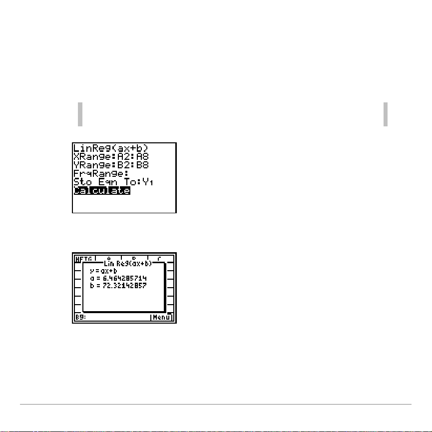
4. At the
Tip
You cannot simply enter Y1 at the Sto Eqn To prompt. You must
select Y1 from the Y-VARS Function menu.
Sto Eqn To
select Y-VARS.
prompt, press
, and then press ato
r
5. Select
Function
y-variable name Y
, and then press
is copied to the prompt.
1
¯
6. Press
¯
2 times to calculate the linear regression.
to select Y1. The
TI-83 Plus CellSheet™ Application Page 58
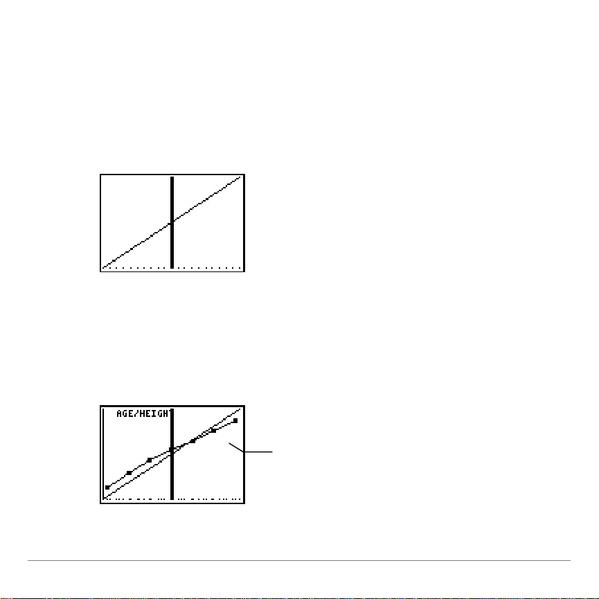
View the graph of the linear regression and the data by
You can see that the
data fits the regression
line well.
displaying the graph of the linear regression and the pic file of
the line chart.
1. Press
2. Press
\
V
two times to exit the application.
to display the graph of the linear regression.
3. Press
4. Press
¯
. The graph is displayed, showing the CellSheet™
\ a a
r
, select
, and then select
Picture
chart and the linear regression.
, select
RecallPic
, and then press
Pic1
.
TI-83 Plus CellSheet™ Application Page 59

Filling a Range
Note
If you enter a formula, it must begin with an = or +.
This spreadsheet contains 25 rows
of data. Each row needed to be
totaled, so the range D1:D25 was
filled with the formula =sum(A1:C1).
Notice that the row numbers in the
formulas automatically
incremented, just as they would
have if the formula had been copied
to the range.
You can fill a range with text, a number, or with a formula. The
range is filled beginning with the top left cell in the range. If you
fill a range with a formula, relative cell references or range
references are adjusted as the range is filled.
1. Select
, and then select
Menu
Options
>
Fill Range
.
2. Enter the spreadsheet range that you want to fill (for
example A1:A10), and then press
¯
3. Enter the text, number, or formula at the
.
Formula
prompt.
4. Press
¯
two times to fill the range.
TI-83 Plus CellSheet™ Application Page 60

Entering a Sequence
1. Select
2. Enter the beginning cell address at the
example,
, and then select
Menu
), and then press
D5
Options
¯
>
Sequence
1st Cell
.
.
prompt (for
3. Enter the arguments for the sequence function at the
prompt, and then press
the sequence
4. Select either
3, 5, 7, 9
Down
or
¯
.)
Right
. (Example:
seq(x,x,3,10,2)
(to enter the number sequence
down the spreadsheet or across the spreadsheet), by
moving the cursor to the option and pressing
5. Press
¯
to return to the spreadsheet and enter the
¯
.
sequence.
seq(
for
TI-83 Plus CellSheet™ Application Page 61

Importing and Exporting Data
Note
When you export data from a range of cells, empty cells in the
range are treated as if they contained the value 0.
Tip
You can enter the list name, or select it from the LIST NAMES
menu (
\
).
Importing Data from a List
1. Select
Import List
Menu
, and then select
.
2. Enter the list name at the
¯
.
Options
List Name
Import/Export
>
>
prompt, and then press
3. Enter the cell address for the first cell where you want the list
imported at the
4. Select
¯
.
1st Cell
Down
to import the list into a column, and then press
prompt, and then press
¯
.
—or—
Select
5. Press
TI-83 Plus CellSheet™ Application Page 62
Right
¯
to import the list into a row.
two times to import the list.

Exporting Data to a List
Note
Exporting data from a row takes much longer than exporting data
from a column.
Tip
You can enter the list name, or select it from the LIST NAMES
menu (
\
).
1. Select
Export List
Menu
, and then select
.
2. Enter the range to export at the
¯
.
3. Enter the list name at the
Options
Range
List Name
prompt.
4. Press
¯
two times to export the list.
Import/Export
>
>
prompt, and then press
TI-83 Plus CellSheet™ Application Page 63

Importing Data from a Matrix
Note
Select the matrix name from the MATRIX NAMES menu (
\
!
).
1. Select
Import Matrix
Menu
, and then select
.
2. Enter the matrix name at the
press
¯
.
Options
Matrix Name
3. Enter the cell address for the first cell where you want the
matrix imported at the
4. Press
¯
two times to import the matrix.
1st Cell
prompt.
Exporting Data to a Matrix
1. Select
Export Matrix
Menu
, and then select
.
Options
2. Enter the range to export at the
¯
.
Import/Export
>
prompt, and then
Import/Export
>
prompt, and then press
Range
>
>
TI-83 Plus CellSheet™ Application Page 64

3. Enter the matrix name at the
Note
Select the matrix name from the MATRIX NAMES menu (
\
!
).
Tip
Press
e
before entering each letter of the name, or press
\
to turn on alpha-lock mode.
Matrix Name
prompt.
4. Press
¯
two times to export the matrix.
Exporting Data to a Variable
1. Select
Export Var
Menu
, and then select
.
2. Enter the cell to export at the
press
¯
.
3. Enter the variable name at the
4. Press
¯
two times to export the data to a variable.
Options
From Cell
Var Name
Import/Export
>
>
prompt, and then
prompt.
TI-83 Plus CellSheet™ Application Page 65

Sorting Data
You can sort columns of data whose cells contain numbers. If
any cell in the column contains a formula or text, the column
cannot be sorted.
1. Select
, and then select
Menu
2. Enter the range to sort at the
3. Select
and pressing
4. Press
¯
Ascend
or
Descend
¯
.
by moving the cursor to the option
again to sort the range.
Options
prompt.
Range
>
Sort
.
TI-83 Plus CellSheet™ Application Page 66

Changing the Column Format
Decimal mode
Description
Float
Floating decimal mode that displays up to 5 digits, plus the
sign and decimal
012345
Fixed decimal mode that specifies the number of digits (
0
through 5) to display to the right of the decimal.
You can change the number of decimal places that are displayed
in each column. The cells display as many digits of the fixed
decimal mode as possible in the given width of the cell.
1. Select
2. Enter the column label (
Menu
, and then select
A, B, C
Options
Col Decimal
>
, etc.), and then press
.
¯
The current decimal mode setting is highlighted.
3. Move the cursor to a decimal mode, and then press
¯
two times to change the mode and return to the spreadsheet.
TI-83 Plus CellSheet™ Application Page 67
.

Working with Charts
Tip
•
You can select a range that you want to chart before you select
the chart type. The range is automatically entered at the
appropriate prompts.
•
Press
¯
to move the cursor to the each subsequent
prompt.
Tip
•
Alpha-lock mode is on when you move the cursor to this
prompt.
•
Entering a title for the chart is optional.
Creating a Scatter Chart
1. Select
, and then select
Menu
Charts
2. Enter the range for the X-coordinates at the
3. Enter the range for the Y-coordinates at the
4. If necessary, enter
YRange2
5. Enter a title for the chart at the
, and
YRange3
Title
>
Scatter
.
prompt.
.
XRange
YRange1
prompt.
prompt.
TI-83 Plus CellSheet™ Application Page 68

6. Select either
Note
If AxesOff is selected on the TI83 Plus format menu (
\
), selecting AxesOn for this chart has no effect.
Note
The DrawFit option changes the window settings so that the
chart is displayed on the screen. If you select Draw, the chart
might be displayed outside of the viewing window.
Note
If necessary, you can change the window settings for the chart.
1. From the CHARTS menu, select
Scatter Window
.
2. Change the values as necessary, and then either select
Draw
to display the chart or select
Save
to save the window settings
and return to the spreadsheet.
AxesOn
, or
AxesOff
(to turn the X and Y axes on
or off) by moving the cursor to the selection and pressing
¯
.
7. Select either
DrawFit
selection and pressing
or
Draw
¯
by moving the cursor to the
. The chart is displayed.
8. To see the X and Y coordinates for each point, press
and then use the arrow keys to move from point to point.
9. Press
\
two times to exit trace mode and return to
the spreadsheet.
U
,
TI-83 Plus CellSheet™ Application Page 69

Example–
Day
Distance Walked
Time
1130
2
1.05
30
3
1.1
30
4
1.15
30
5
1.2
30
6
2.0
45
7
2.0
45
8
1.3
30
9
1.35
30
10
1.4
30
progress. Enter the following data into a spreadsheet,
calculate minutes per mile for each day, and then create a
chart that shows her progress.
Enter the spreadsheet headings and data.
A person starts walking for exercise and charts her
1. Create a new spreadsheet file
2. Enter the following headings
MIN/MILE
TI-83 Plus CellSheet™ Application Page 70
.
named
in cells A1:D1:
WALKING
DAY, DIST, TIME
.
,

3. Enter the sequence 1:10 in cells A2:A11. The arguments for
the function are
X,X,1,10
(you are entering the sequence X
where X is the variable from 1 to 10).
4. Your spreadsheet should look like this:
5. Enter the data for the
DIST
and
columns from the table
TIME
above.
Calculate the number of minutes per mile that the person
walked on each day in column D.
1. Move the cursor to cell D2, and enter the formula
2. Copy the formula
TI-83 Plus CellSheet™ Application Page 71
in cell D2 to cells D3:D11.
=C2/B2
.

Your spreadsheet should look like this:
Tip
Press
¯
to move the cursor to each subsequent prompt.
Create a scatter chart for the data using the DAY column for
XRange, and the MIN/MI column for the YRange.
1. Select
2. Enter
A2:A11
, and then select
Menu
at the
XRange
Charts
prompt.
>
Scatter
.
TI-83 Plus CellSheet™ Application Page 72
3. Enter
D2:D11
at the
YRange1
prompt.
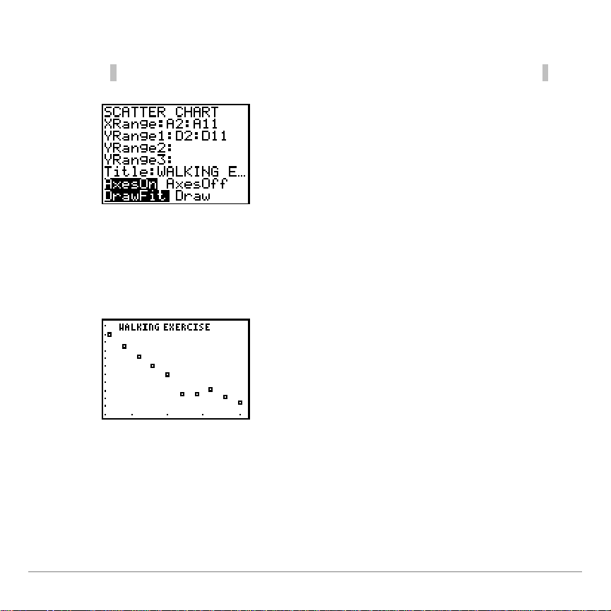
4. Enter
Tip
Alpha-lock mode is on when the cursor is at this prompt.
WALK
at the
prompt.
Title
5. Press
6. Press
¯
U
two times to display the scatter chart.
, and then use the arrow keys to move from
point to point and display the data values.
7. Press
\
two times to exit trace mode and return to
the spreadsheet.
TI-83 Plus CellSheet™ Application Page 73

Creating a Line Chart
Tip
•
You can select a range that you want to chart before you select
the chart type. The range is automatically entered at the
appropriate prompts.
•
Press
¯
to move the cursor to each subsequent prompt.
Tip
Alpha-lock mode is on when you move the cursor to this prompt.
1. Select
, and then select
Menu
Charts
>
2. Enter the range for the X-coordinates at the
(for example A2:A11), and then press
3. Enter the range for the Y-coordinates at the
(for example B2:B11).
4. If necessary, enter
YRange2
5. Enter a title for the chart at the
, and
YRange3
prompt.
Title
6. Select either
AxesOn
, or
AxesOff
(to turn the X and Y axes on
or off) by moving the cursor to the selection and pressing
¯
.
.
Line
¯
.
XRange
.
YRange1
prompt
prompt
TI-83 Plus CellSheet™ Application Page 74
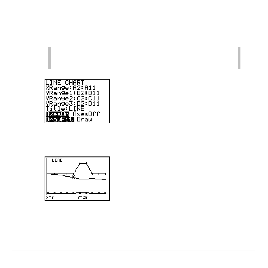
7. Select either
Tip
The DrawFit option changes the window settings so that the
chart is displayed on the screen. If you select Draw, the chart
might be displayed outside of the viewing window.
DrawFit
or
(to select the window settings
Draw
for the drawing) by moving the cursor to the selection and
pressing
¯
. The chart is displayed.
8. Press
U
and use the arrow keys to view the data
elements.
TI-83 Plus CellSheet™ Application Page 75

9. Press
Note
If necessary, you can change the window settings for the chart.
1. From the CHARTS menu, select
Scatter Window
.
2. Change the values as necessary, and then either select
Draw
to display the chart or select
Save
to save the window settings
and return to the spreadsheet.
Tip
•
You can select a range that you want to chart before you select
the chart type. The range is automatically entered at the
appropriate prompts.
•
Press
¯
to move the cursor to each subsequent prompt.
Tip
Alpha-lock mode is on when you move the cursor to this prompt.
\
twice to return to the spreadsheet.
Creating a Bar Chart
1. Select
, and then select
Menu
Charts
>
2. Enter the range for the category labels at the
prompt, and then press
¯
.
3. Enter the range for the first category at the
and then press
¯
.
4. Enter a name for the first category at the
.
Bar
Ser1Name
Categories
Series1
prompt,
prompt.
TI-83 Plus CellSheet™ Application Page 76

5. Enter the range for the second category at the
Tip
Alpha-lock mode is on when you move the cursor to this prompt.
Tip
You can return to the
BAR CHART
screen later and change the
display without having to enter the other parameters again.
Series2
prompt.
6. Enter a name for the second category at the
prompt.
7. If necessary, enter the range for the third category at the
prompt.
Series3
8. If necessary, enter a name for the third category at the
Ser3Name
9. Enter a title for the chart at the
prompt.
prompt.
Title
10. Select either
Vertical
, or
(to display the chart either
Horiz
vertically or horizontally) by moving the cursor to the
selection and pressing
¯
.
Ser2Name
TI-83 Plus CellSheet™ Application Page 77

11. Select either
Tip
•
The DrawFit option changes the window settings so that the
chart is displayed on the screen. If you select Draw, the chart
might be displayed outside of the viewing window.
•
If the entire chart will not fit on one screen, arrows are
displayed on the left side of the screen. Press the arrow keys
to view the part of the chart that is not currently displayed.
Note
If necessary, you can change the window settings for the chart.
1. From the CHARTS menu, select
Scatter Window
.
2. Change the values as necessary, and then either select
Draw
to display the chart or select
Save
to save the window settings
and return to the spreadsheet.
DrawFit
or
(to select the window settings
Draw
for the drawing) by moving the cursor to the selection and
pressing
¯
. The chart is displayed.
12. Press
U
and use the arrow keys to view the data
elements.
13. Press
\
twice to return to the spreadsheet.
TI-83 Plus CellSheet™ Application Page 78

Month
1999
2000
Jan3027
Feb3436
Mar3544
Apr5146
May6066
Jun6657
Jul7174
Aug7175
Sep6273
Oct5053
Nov4439
Dec3523
Example–
Create a bar chart that shows the following average
temperatures (in degrees Fahrenheit) for each month in a
particular area for the years 1999 and 2000.
1. Create a new spreadsheet file named
2. Enter the headings
MONTH, 1999
, and
TEMPS
2000
.
in cells A1:C1.
3. Enter the data in the MONTH, 1999, and 2000 columns from
the table
TI-83 Plus CellSheet™ Application Page 79
above.

Your spreadsheet should look like this:
Tip
Press
¯
to move the cursor to each subsequent prompt.
Note
Press
e
to turn the alpha-lock mode off.
Create a bar chart for the data using A2:A13 as the
categories, B2:B13 as the first series, and C2:C13 as the
second series.
1. Enter
A2:A13
at the
Categories
prompt.
2. Enter
3. Enter
B2:B13
1999
at the
at the
Series1
Ser1Name
prompt.
prompt.
TI-83 Plus CellSheet™ Application Page 80
4. Enter
C2:C13
at the
Series2
prompt.

Note
Press
e
to turn the alpha-lock mode off.
Tip
Alpha-lock mode is on when you move the cursor to this prompt.
5. Enter
2000
at the
Ser2Name
prompt.
6. Enter
TEMPS
at the Title prompt.
7. Press
TI-83 Plus CellSheet™ Application Page 81
¯
two times to display the chart.

8. Press
Tip
Press
¯
to move the cursor to each subsequent prompt.
Tip
You can select a range that you want to chart before you select
the chart type. The range is automatically entered at the
appropriate prompts.
U
, and then press the arrow keys to display the
data and labels for each bar.
9. Press
\
two times to return to the spreadsheet.
Creating a Pie Chart
1. Select
, and then select
Menu
Charts
2. Enter the range for the category labels at the
>
Pie
.
Categories
prompt.
3. Enter the range for the chart at the
Series
prompt.
TI-83 Plus CellSheet™ Application Page 82

4. Select
Tip
•
If you select Number, the data from the spreadsheet is
displayed in the pie chart.
•
If you select Percent, the percentage of the whole that each
data element makes up is displayed in the pie chart.
Tip
Alpha-lock mode is on when you move the cursor to this prompt.
Area
Cats
Dogs
Fish
13220
3
21215
7
357
9
41714
12
Number
and pressing
or
Percent
¯
by moving the cursor to the option
.
5. Enter a title for the chart at the
Title
prompt.
6. Select
Example–
to display the chart.
Draw
The following data was gathered about the types of
pets that are found in homes in four different areas of a city.
Display a pie chart that shows the numbers of households in
the city that have each pet and the percentages of households
in each area that have pets.
TI-83 Plus CellSheet™ Application Page 83

Enter the headings and data for the spreadsheet.
1. Create a new spreadsheet file
2. Enter the headings
AREA, CATS, DOGS
named
PETS
, and
.
FISH
into cells
A1:D1.
3. Enter the data
from the table above below the headings in
the spreadsheet.
Your spreadsheet should look like this:
Calculate the number of each type of pet in the city and the
number of pets in each area.
1. Enter the sum
of the CATS column in cell B6.
2. Copy the formula
3. Enter the sum
TI-83 Plus CellSheet™ Application Page 84
to cells C6 and D6.
of pets in Area 1 of the city in cell E2.

4. Copy the formula to cells E3:E5.
Tip
Press
¯
to move the cursor to each subsequent prompt.
Your spreadsheet should look like this:
Create a pie chart that shows the number of the types of pets
in the households.
1. Select
2. Enter the range for the category labels at the
prompt (
, and then select
Menu
B1:D1
).
Charts
>
Pie
.
Categories
TI-83 Plus CellSheet™ Application Page 85
3. Enter the range for the data (
4. Select
pressing
Number
¯
5. Enter the title
by moving the cursor to the option and
.
at the
PETS
B6:D6
prompt.
Title
) at the
Series
prompt.

6. Press
¯
again to display the chart.
7. Press
U
and use the arrow keys to display the category
labels.
8. Press
Create a pie chart that shows the percentage of households
\
two times to exit the pie chart.
that have pets by city area.
1. Select
, and then select
Menu
Charts
2. Enter the range for the category labels at the
prompt (
TI-83 Plus CellSheet™ Application Page 86
A2:A5
).
>
Pie
.
Categories

3. Enter the range for the data (
E2:E5
) at the
Series
prompt.
4. Select
pressing
Percent
¯
5. Enter the title
6. Press
7. Press
¯
U
labels.
8. Press
\
by moving the cursor to the option and
.
AREAS
at the
prompt.
Title
again to display the chart.
and use the arrow keys to display the category
two times to exit the pie chart.
TI-83 Plus CellSheet™ Application Page 87

Examples
Planet
Gravitational factor
M (Mercury)
0.38
V (Venus)
0.91
E (Earth)
1
M (Mars)
0.38
J (Jupiter)
2.54
S (Saturn)
1.08
U (Uranus)
0.91
N (Neptune)
1.19
P (Pluto)
0.06
Example 1–
on Earth weigh on each of the nine planets?
Enter the headings and data into the spreadsheet.
1. Create a new spreadsheet file
2. Enter the following spreadsheet headings
PLANET
GRAV
WT
– weight
3. Enter the following data
How much would a person who weighs 125 pounds
named
GRAVITY
.
in cells A1:C1.
– planet name
– gravitational factor
for the first two columns.
TI-83 Plus CellSheet™ Application Page 88

4. Enter
in cell C4.
125
Your spreadsheet should look like this:
Calculate the weight of the 125-pound person on the rest of
the planets.
1. Enter the formula
2. Copy the formula
3. Copy the formula
TI-83 Plus CellSheet™ Application Page 89
=$C$444B2
in cell C2 to cell C3
in cell C3 to cells C5:C10.
in cell C2.
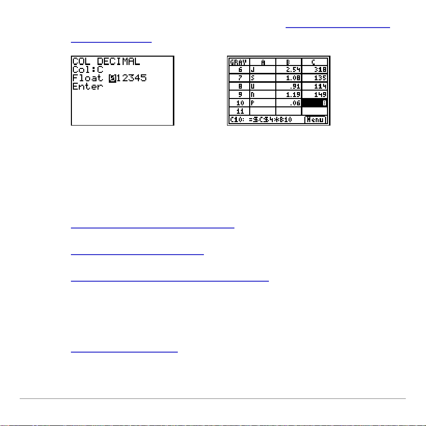
4. To view the weights as whole numbers change the column
decimal format to 0.
Example 2–
Make a chart of interest earned on $1000 at 6% per
year.
1. Create a new spreadsheet file
2. Enter the reference data
, 1000 in cell A1, and .06 in cell A2.
3. Enter the following column headings
YEAR
– the number of years that the principle has earned
named
INTEREST
.
in cells B1:C1.
interest.
– the sum of the principal and the interest
BAL
4. Enter the sequence
TI-83 Plus CellSheet™ Application Page 90
1 – 10 in cells B2:B11.
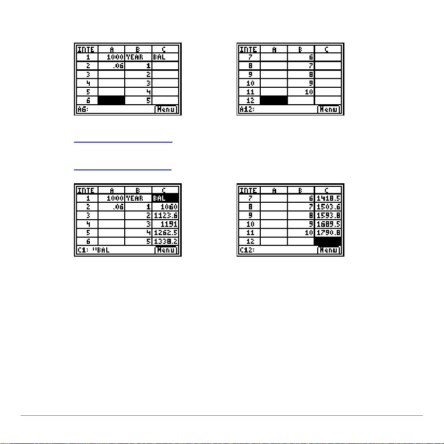
Your spreadsheet should look like this:
5. Enter the formula
6. Copy the formula
=$A$1(1+$A$2)^B2
in cell C2 to cells C3:C11.
in cell C2.
TI-83 Plus CellSheet™ Application Page 91

Example 3–
Secant line
Tangent line
f
Examine the relationship between the slope of a
secant line on a curve and a tangent line to the curve.
What is the slope of the tangent line of f(x) = x2at x = 3?
Compare the slope of the secant line to the tangent line as the
point (x+h,f(x+h)) gets closer to the point (x,f(x)) at x = 3. The
derivative of the function at x = 3 is the slope of the tangent line.
TI-83 Plus CellSheet™ Application Page 92

1. Create a new spreadsheet file named
X
value of x
H(RHS)
value of h from the right hand side
X+H
value of x+h
SEC SLP
slope of the secant line
TAN SLP
slope of the tangent line which will be calculated using the
derivative f'(3) = 243 = 6
TAN SEC
slope of the tangent line minus the slope of the secant line
2. Enter the following headings in cells A1:F1:
You need to begin the comparison with h a large distance
away from x. As h gets closer to x, you can see a trend
develop. For this example, begin with h = 100, with each
subsequent h value 1/10 of the preceding h value.
DERIV
.
3. Enter
for x in cells A2 through A16 using the fill range
3
option.
TI-83 Plus CellSheet™ Application Page 93

4. Enter
100
in cell B2 for the initial value of h.
5. Enter the formula
6. Copy the formula
7. Enter the formula
8. Copy the formula
9. Enter the formula
=B2/10
from cell B3 to cells B4 through B16.
=A2+B2
from cell C2 to cells C3 through C16.
=(C2^2-A2^2)/B2
secant line).
10. Copy the formula
11. Enter the formula
12. Copy the formula
13. Enter the formula
from cell D2 to cells D3 through D16.
=2ggA2
from cell E2 to cells E3 through E16.
=E211D2
the secant and tangent lines).
14. Copy the formula
from cell F2 to cells F3 through F16.
in cell B3.
in cell C2.
in cell D2 (slope of the
in cell E2 (slope of the tangent line).
in cell F2 (difference in the slope of
TI-83 Plus CellSheet™ Application Page 94
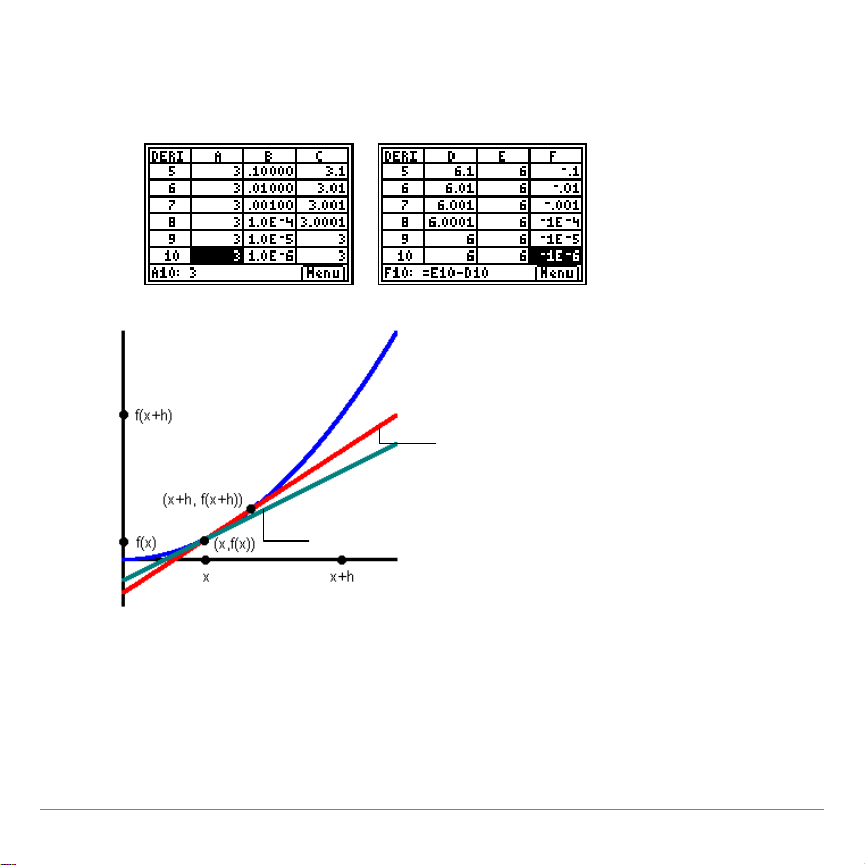
You can see that as h gets smaller (and thus, x + h gets closer
Tangent line
Secant line
to x), the slope of the secant line gets closer to the slope of the
tangent line.
TI-83 Plus CellSheet™ Application Page 95

Example 4–
Fibonacci
The first two terms are 1 and 1, and each succeeding term is
the sum of the two immediately preceding terms.
Squares
Squares each term in the whole number series, beginning
with 1.
Which one increases faster, Fibonacci number or
the sequence of squares?
Enter the headings and the first list of data.
1. Create a new spreadsheet file
2. Enter the following headings
named
in cells A1:C1.
FIB
.
NUMS – whole numbers
FIBS – Fibonacci numbers
SQUARES – squares
3. Use the sequence option
to fill cells A2:A19 with the
sequence of whole numbers {1,2,3, …, 18}.
TI-83 Plus CellSheet™ Application Page 96

Your spreadsheet should look like this:
Set up the data for the FIBS column.
1. Enter
2. Enter the formula
3. Copy the formula
in cells B2 and B3.
1
=B2+B3
to cells B5:B19.
in cell B4.
TI-83 Plus CellSheet™ Application Page 97

Set up the data for the SQUARES column.
You can see that the
Fibonacci numbers
increase much more
rapidly than the squares
after the 12thstep.
1. Enter the formula
2. Copy the formula
2
in cell C2.
=A2
to cells C3:C19.
Your spreadsheet should look like this:
TI-83 Plus CellSheet™ Application Page 98

Errors, Error Messages, and Restrictions
Message
Description
INVALID CELL, INVALID
RANGE.
This occurs when you type in an invalid cell
or a range such as A0, BZ12, or A1:A1000.
Valid cells are A1 to Z999.
CIRCLE REF
This occurs when the logic of cell formulas
results in a loop, for example when A1 is
set to =A1.
CANNOT SORT
The CellSheet™ application does not sort
ranges that contain formulas.
INVALID NAME
The name that you entered is too long, or
contains characters that are invalid.
Each cell that contains a formula displays
error in any cell formula to alert you that an error exists. The
error is always in the last cell that you entered or edited.
If the error is in a cell that contains a formula, you do not have to
correct the error immediately. You can continue editing the
spreadsheet without making a correction. However, if the error is
in a cell that does not contain a formula, you must correct the
error before you can continue editing the spreadsheet.
ERROR
if there is an
TI-83 Plus CellSheet™ Application Page 99

Message
Description
INVALID LIST, INVALID
MATRIX, INVALID VAR
The list name, matrix name, or variable
name does not exist.
SYNTAX
This occurs when you enter an invalid cell
reference (e.g., A0), or if you delete a cell
that is referred to by another cell.
If you encounter error messages that are not listed above, check
the TI83 Plus
manual for more information.
TI-83 Plus CellSheet™ Application Page 100
 Loading...