

Page 1

TI-83
GRAPHING CALCULATOR
GUIDEBOOK
TI-GRAPH LINK, Calculator-Based Laboratory, CBL, CBL 2, Calculator-Based Ranger, CBR,
Constant Memory, Automatic Power Down, APD, and EOS are trademarks of Texas
Instruments Incorporated.
IBM is a registered trademark of International Business Machines Corporation.
Macintosh is a registered trademark of Apple Computer, Inc.
Windows is a registered trademark of Microsoft Corporation.
© 1996, 2000, 2001 Texas Instruments Incorporated.
Page 2

Important
US FCC
Information
Concerning
Radio Frequency
Interference
Texas Instruments makes no warranty, either expressed or
implied, including but not limited to any implied warranties of
merchantability and fitness for a particular purpose, regarding any
programs or book materials and makes such materials available
solely on an “as-is” basis.
In no event shall Texas Instruments be liable to anyone for special,
collateral, incidental, or consequential damages in connection with
or arising out of the purchase or use of these materials, and the
sole and exclusive liability of Texas Instruments, regardless of the
form of action, shall not exceed the purchase price of this
equipment. Moreover, Texas Instruments shall not be liable for any
claim of any kind whatsoever against the use of these materials by
any other party.
This equipment has been tested and found to comply with the
limits for a Class B digital device, pursuant to Part 15 of the FCC
rules. These limits are designed to provide reasonable protection
against harmful interference in a residential installation. This
equipment generates, uses, and can radiate radio frequency energy
and, if not installed and used in accordance with the instructions,
may cause harmful interference with radio communications.
However, there is no guarantee that interference will not occur in
a particular installation.
If this equipment does cause harmful interference to radio or
television reception, which can be determined by turning the
equipment off and on, you can try to correct the interference by
one or more of the following measures:
• Reorient or relocate the receiving antenna.
• Increase the separation between the equipment and receiver.
• Connect the equipment into an outlet on a circuit different
from that to which the receiver is connected.
• Consult the dealer or an experienced radio/television
technician for help.
Caution: Any changes or modifications to this equipment not
expressly approved by Texas Instruments may void your authority
to operate the equipment.
Page 3

Table of Contents
This manual describes how to use the TI.83 Graphing Calculator. Getting
Started is an overview of TI.83 features. Chapter 1 describes how the TI.83
operates. Other chapters describe various interactive features. Chapter 17
shows how to combine these features to solve problems.
Getting Started: Do This First!
TI-83 Keyboard
TI-83 Menus
First Steps
Entering a Calculation: The Quadratic Formula
Converting to a Fraction: The Quadratic Formula
Displaying Complex Results: The Quadratic Formula
Defining a Function: Box with Lid
Defining a Table of Values: Box with Lid
Zooming In on the Table: Box with Lid
Setting the Viewing Window: Box with Lid
Displaying and Tracing the Graph: Box with Lid
Zooming In on the Graph: Box with Lid
Finding the Calculated Maximum: Box with Lid
Other TI-83 Features
..........................................
.............................................
...............................................
..........
........
....
.......................
.................
...................
...............
.........
..................
..........
.....................................
2
4
5
6
7
8
9
10
11
12
13
15
16
17
Chapter 1: Operating the TI-83
Turning On and Turning Off the TI-83
Setting the Display Contrast
The Display
..............................................
.............................
Entering Expressions and Instructions
TI-83 Edit Keys
Setting Modes
Using TI-83 Variable Names
Storing Variable Values
Recalling Variable Values
(Last Entry) Storage Area
ENTRY
(Last Answer) Storage Area
Ans
TI-83 Menus
and
VARS
..........................................
...........................................
.............................
..................................
................................
........................
.........................
.............................................
Menus
VARS Y.VARS
.........................
Equation Operating System (EOSé)
Error Conditions
.........................................
....................
...................
.....................
1-2
1-3
1-4
1-6
1-8
1-9
1-13
1-14
1-15
1-16
1-18
1-19
1-21
1-22
1-24
Introduction iii
Page 4

Chapter 2: Math, Angle, and Test Operations
Getting Started: Coin Flip
Keyboard Math Operations
Operations
MATH
Using the Equation Solver
MATH NUM
(Number) Operations
................................
..............................
........................................
...............................
........................
Entering and Using Complex Numbers
MATH CPX
MATH PRB
ANGLE
TEST
TEST LOGIC
(Complex) Operations
(Probability) Operations
Operations
(Relational) Operations
(Boolean) Operations
.......................................
.......................
............................
......................
...................
.....................
2-2
2-3
2-5
2-8
2-13
2-16
2-18
2-20
2-23
2-25
2-26
Chapter 3: Function Graphing
Chapter 4: Parametric Graphing
Chapter 5: Polar Graphing
Getting Started: Graphing a Circle
Defining Graphs
Setting the Graph Modes
Defining Functions
.........................................
.................................
......................................
Selecting and Deselecting Functions
Setting Graph Styles for Functions
Setting the Viewing Window Variables
Setting the Graph Format
Displaying Graphs
................................
.......................................
.......................
.....................
.......................
...................
Exploring Graphs with the Free-Moving Cursor
Exploring Graphs with
Exploring Graphs with the
Using
ZOOM MEMORY
Using the
(Calculate) Operations
CALC
Getting Started: Path of a Ball
Defining and Displaying Parametric Graphs
Exploring Parametric Graphs
Getting Started: Polar Rose
Defining and Displaying Polar Graphs
Exploring Polar Graphs
...........................
TRACE
..................................
..................................
Instructions
ZOOM
..................
...........................
..............
............................
..............................
...................
..........
...........
3-2
3-3
3-4
3-5
3-7
3-9
3-11
3-13
3-15
3-17
3-18
3-20
3-23
3-25
4-2
4-4
4-7
5-2
5-3
5-6
iv Introduction
Page 5

Chapter 6: Sequence Graphing
Getting Started: Forest and Trees
Defining and Displaying Sequence Graphs
Selecting Axes Combinations
Exploring Sequence Graphs
Graphing Web Plots
......................................
Using Web Plots to Illustrate Convergence
Graphing Phase Plots
....................................
........................
...............
............................
..............................
...............
Comparing TI-83 and TI.82 Sequence Variables
Keystroke Differences Between TI-83 and TI-82
..........
.........
6-2
6-3
6-8
6-9
6-11
6-12
6-13
6-15
6-16
Chapter 7: Tables
Chapter 8: DRAW Operations
Chapter 9: Split Screen
Getting Started: Roots of a Function
Setting Up the Table
.....................................
Defining the Dependent Variables
Displaying the Table
.....................................
.....................
........................
Getting Started: Drawing a Tangent Line
Using the
DRAW
Clearing Drawings
Drawing Line Segments
Drawing Horizontal and Vertical Lines
Drawing Tangent Lines
Drawing Functions and Inverses
Shading Areas on a Graph
Drawing Circles
Placing Text on a Graph
Using Pen to Draw on a Graph
Drawing Points on a Graph
Drawing Pixels
Storing Graph Pictures (
Recalling Graph Pictures (
Storing Graph Databases (
Recalling Graph Databases (
...................................
Menu
.......................................
..................................
...................
..................................
.........................
...............................
..........................................
.................................
...........................
..............................
..........................................
.............................
)
Pic
...........................
)
Pic
.........................
)
GDB
.......................
)
GDB
Getting Started: Exploring the Unit Circle
Using Split Screen
(Horizontal) Split Screen
Horiz
(Graph-Table) Split Screen
G-T
TI.83 Pixels in
.......................................
...........................
..........................
Horiz
and
G-T
.....................
Modes
.................
................
7-2
7-3
7-4
7-5
8-2
8-3
8-4
8-5
8-6
8-8
8-9
8-10
8-11
8-12
8-13
8-14
8-16
8-17
8-18
8-19
8-20
9-2
9-3
9-4
9-5
9-6
Introduction v
Page 6

Chapter 10: Matrices
Getting Started: Systems of Linear Equations
Defining a Matrix
Viewing and Editing Matrix Elements
Using Matrices with Expressions
Displaying and Copying Matrices
Using Math Functions with Matrices
Using the
........................................
....................
........................
........................
.....................
MATRX MATH
Operations
.....................
............
10-2
10-3
10-4
10-7
10-8
10-9
10-12
Chapter 11: Lists
Chapter 12: Statistics
Chapter 13: Inferential Statistics and Distributions
Getting Started: Generating a Sequence
Naming Lists
Storing and Displaying Lists
Entering List Names
.............................................
.............................
.....................................
Attaching Formulas to List Names
Using Lists in Expressions
Menu
LIST OPS
LIST MATH
..........................................
Menu
........................................
...............................
..................
.......................
Getting Started: Pendulum Lengths and Periods
Setting up Statistical Analyses
Using the Stat List Editor
Attaching Formulas to List Names
Detaching Formulas from List Names
Switching Stat List Editor Contexts
Stat List Editor Contexts
Menu
STAT EDIT
........................................
Regression Model Features
Menu
STAT CALC
Statistical Variables
........................................
......................................
Statistical Analysis in a Program
Statistical Plotting
.......................................
Statistical Plotting in a Program
...........................
................................
.......................
....................
......................
.................................
..............................
.........................
.........................
Getting Started: Mean Height of a Population
Inferential Stat Editors
STAT TESTS
Menu
Inferential Statistics Input Descriptions
Test and Interval Output Variables
Distribution Functions
Distribution Shading
...................................
......................................
..................
.......................
...................................
.....................................
.........
............
11-2
11-3
11-4
11-6
11-7
11-9
11-10
11-17
12-2
12-10
12-11
12-14
12-16
12-17
12-18
12-20
12-22
12-24
12-29
12-30
12-31
12-37
13-2
13-6
13-9
13-26
13-28
13-29
13-35
vi Introduction
Page 7

Chapter 14: Financial Functions
Getting Started: Financing a Car
Getting Started: Computing Compound Interest
Using the
TVM Solver
....................................
Using the Financial Functions
Calculating Time Value of Money (
Calculating Cash Flows
..................................
Calculating Amortization
Calculating Interest Conversion
.........................
..........
...........................
.................
)
TVM
................................
..........................
Finding Days between Dates/Defining Payment Method
Using the
TVM
Variables
.................................
.....
14-2
14-3
14-4
14-5
14-6
14-8
14-9
14-12
14-13
14-14
Chapter 15: CATALOG, Strings, Hyperbolic Functions
Chapter 16: Programming
Chapter 17: Applications
Browsing the TI-83
CATALOG
Entering and Using Strings
Storing Strings to String Variables
String Functions and Instructions in the
Hyperbolic Functions in the
Getting Started: Volume of a Cylinder
Creating and Deleting Programs
Entering Command Lines and Executing Programs
Editing Programs
........................................
Copying and Renaming Programs
PRGM CTL
PRGM I/O
(Control) Instructions
(Input/Output) Instructions
Calling Other Programs as Subroutines
Comparing Test Results Using Box Plots
Graphing Piecewise Functions
Graphing Inequalities
....................................
Solving a System of Nonlinear Equations
Using a Program to Create the Sierpinski Triangle
Graphing Cobweb Attractors
Using a Program to Guess the Coefficients
Graphing the Unit Circle and Trigonometric Curves
Finding the Area between Curves
Using Parametric Equations: Ferris Wheel Problem
...........................
...............................
.......................
CATALOG
CATALOG
...........................
............................
..................
....................
.........................
........................
.......................
...................
..................
................
................
...............
........................
......
......
.......
......
......
Demonstrating the Fundamental Theorem of Calculus
Computing Areas of Regular N-Sided Polygons
Computing and Graphing Mortgage Payments
..........
...........
...
15-2
15-3
15-4
15-6
15-10
16-2
16-4
16-5
16-6
16-7
16-8
16-16
16-22
17-2
17-4
17-5
17-6
17-7
17-8
17-9
17-10
17-11
17-12
17-14
17-16
17-18
Introduction vii
Page 8

Chapter 18: Memory Management
Checking Available Memory
Deleting Items from Memory
.............................
............................
Clearing Entries and List Elements
Resetting the TI.83
......................................
......................
18-2
18-3
18-4
18-5
Chapter 19: Communication Link
Appendix A: Tables and Reference Information
Appendix B: General Information
Index
Getting Started: Sending Variables
TI-83
Selecting Items to Send
Receiving Items
Transmitting Items
Transmitting Lists to a TI-82
...............................................
LINK
..................................
..........................................
.......................................
.............................
Transmitting from a TI-82 to a TI-83
Backing Up Memory
.....................................
Table of Functions and Instructions
Menu Map
Variables
Statistical Formulas
Financial Formulas
Battery Information
In Case of Difficulty
Error Conditions
Accuracy Information
Support and Service Information
Warranty Information
...............................................
................................................
.....................................
......................................
......................................
.....................................
.........................................
....................................
.........................
....................................
.......................
.....................
.....................
19-2
19-3
19-4
19-5
19-6
19-8
19-9
19-10
A-2
A-39
A-49
A-50
A-54
B-2
B-4
B-5
B-10
B-12
B-13
viii Introduction
Page 9

Getting Started: Do This First!
Contents
TI-83 Keyboard
TI-83 Menus
First Steps
Entering a Calculation: The Quadratic Formula
Converting to a Fraction: The Quadratic Formula
..........................................
.............................................
...............................................
..........
........
Displaying Complex Results: The Quadratic Formula
Defining a Function: Box with Lid
Defining a Table of Values: Box with Lid
Zooming In on the Table: Box with Lid
Setting the Viewing Window: Box with Lid
Displaying and Tracing the Graph: Box with Lid
Zooming In on the Graph: Box with Lid
Finding the Calculated Maximum: Box with Lid
Other TI.83 Features
.....................................
.......................
.................
...................
...............
.........
..................
..........
....
2
4
5
6
7
8
9
10
11
12
13
15
16
17
Getting Started 1
Page 10

TI-83 Keyboard
Generally, the keyboard is divided into these zones: graphing keys, editing
keys, advanced function keys, and scientific calculator keys.
Keyboard Zones
Graphing Keys
Graphing keys access the interactive graphing features.
Editing keys allow you to edit expressions and values.
Advanced function keys display menus that access the
advanced functions.
Scientific calculator keys access the capabilities of a
standard scientific calculator.
Editing Keys
Advanced
Function Keys
Scientific
Calculator Keys
2 Getting Started
Page 11

Using the Color-Coded Keyboard
The keys on the TI.83 are color-coded to help you easily
locate the key you need.
The gray keys are the number keys. The blue keys along the
right side of the keyboard are the common math functions.
The blue keys across the top set up and display graphs.
The primary function of each key is printed in white on the
key. For example, when you press
, the
MATH
menu is
displayed.
Using the
and
y
ƒ
Keys
The y key accesses
the second function
printed in yellow above
each key.
The secondary function of each key is printed in yellow
above the key. When you press the yellow y key, the
character, abbreviation, or word printed in yellow above
the other keys becomes active for the next keystroke. For
example, when you press y and then
, the
TEST
menu is displayed. This guidebook describes this keystroke
combination as y [
TEST
].
The alpha function of each key is printed in green above
the key. When you press the green
ƒ
key, the alpha
character printed in green above the other keys becomes
active for the next keystroke. For example, when you press
ƒ
and then
guidebook describes this keystroke combination as
A
].
[
, the letter
A is entered. This
ƒ
The ƒ key
accesses the alpha
function printed in
green above each key.
Getting Started 3
Page 12

A
TI-83 Menus
Displaying a Menu
While using your TI.83, you often will need
to access items from its menus.
When you press a key that displays a menu,
that menu temporarily replaces the screen
where you are working. For example, when
you press
as a full screen.
fter you select an item from a menu, the
screen where you are working usually is
displayed again.
Moving from One Menu to Another
Some keys access more than one menu. When
you press such a key, the names of all
accessible menus are displayed on the top
line. When you highlight a menu name, the
items in that menu are displayed. Press ~ and
|
to highlight each menu name.
Selecting an Item from a Menu
The number or letter next to the current menu
item is highlighted. If the menu continues
beyond the screen, a down arrow (
replaces the colon (
item. If you scroll beyond the last displayed
item, an up arrow (
the first item displayed.You can select an item
in either of two ways.
¦
Press † or } to move the cursor to the
number or letter of the item; press
¦
Press the key or key combination for the
number or letter next to the item.
, the
menu is displayed
MATH
:
) in the last displayed
#
) replaces the colon in
$
)
Í
.
Leaving a Menu without Making a Selection
You can leave a menu without making a
selection in any of three ways.
¦
Press
‘
to return to the screen
where you were.
¦
Press y [
QUIT
] to return to the home
screen.
¦
Press a key for another menu or screen.
4 Getting Started
Page 13

First Steps
Before starting the sample problems in this chapter, follow the steps on this
page to reset the TI.83 to its factory settings and clear all memory. This
ensures that the keystrokes in this chapter will produce the illustrated results.
To reset the TI.83, follow these steps.
1. Press É to turn on the calculator.
2. Press and release y, and then press
MEM
[
] (above Ã).
When you press y, you access the
operation printed in yellow above the next
key that you press. [
y
operation of the à key.
The
MEMORY
3. Press 5 to select 5:Reset.
The
menu is displayed.
RESET
4. Press 1 to select 1:All Memory.
The
RESET MEMORY
MEM
] is the
menu is displayed.
menu is displayed.
5. Press 2 to select 2:Reset.
All memory is cleared, and the calculator
is reset to the factory default settings.
When you reset the TI.83, the display
contrast is reset.
¦
If the screen is very light or blank, press
and release y, and then press and
hold } to darken the screen.
¦
If the screen is very dark, press and
release y, and then press and hold
to lighten the screen.
†
Getting Started 5
Page 14

Entering a Calculation: The Quadratic Formula
Use the quadratic formula to solve the quadratic equations 3X2 + 5X + 2 = 0
2
and 2X
1. Press
2. Press
3. Press
4. Press
N X + 3 = 0. Begin with the equation 3X2 + 5X + 2 = 0.
¿ ƒ
3
[A] (above
store the coefficient of the X
ƒ
:
] (above Ë). The colon
[
2
term.
) to
allows you to enter more than one
instruction on a line.
¿ ƒ
5
[B] (above
store the coefficient of the X
ƒ
the same line. Press
(above
:
[
] to enter a new instruction on
¿ ƒ
2
) to store the constant.
Í
to store the values to the
term. Press
[C]
) to
variables A, B, and C.
The last value you stored is shown on the
right side of the display. The cursor moves
to the next line, ready for your next entry.
5. Press £ Ì
¡ ¹
ƒ
ƒ
[B] Ã y [‡]
ƒ
4
A
[
] ¤ to enter the expression for
[A]
ƒ
[C] ¤ ¤ ¥ £ 2
one of the solutions for the quadratic
formula,
2
−
6. Press
equation 3X
4
+−
bb ac
2
a
Í
to find one solution for the
2
+ 5X + 2 = 0.
The answer is shown on the right side of
the display. The cursor moves to the next
line, ready for you to enter the next
expression.
6 Getting Started
ƒ
[B]
Page 15

Converting to a Fraction: The Quadratic Formula
You can show the solution as a fraction.
1. Press
to display the
MATH
menu.
2. Press 1 to select 1:
4
Frac from the
MATH
menu.
When you press
the home screen.
1, Ans4Frac is displayed on
Ans is a variable that
contains the last calculated answer.
3. Press
Í
to convert the result to a
fraction.
To save keystrokes, you can recall the last expression you entered, and then
edit it for a new calculation.
4. Press y [
ENTRY
] (above
Í
) to recall
the fraction conversion entry, and then
press y [
ENTRY
] again to recall the
quadratic-formula expression,
2
−
bb ac
4
+−
2
a
5. Press } to move the cursor onto the + sign
in the formula. Press ¹ to edit the
quadratic-formula expression to become:
2
−
6. Press
the quadratic equation 3X
4
−−
bb ac
2
a
Í
to find the other solution for
2
+ 5X + 2 = 0.
Getting Started 7
Page 16

Displaying Complex Results: The Quadratic Formula
Now solve the equation 2X2 N X + 3 = 0. When you set a+b
mode, the TI.83 displays complex results.
1. Press
z † † † † † †
(6 times), and
then press ~ to position the cursor over
a+b
i
. Press
Í
to select
a+b
i
complex-
number mode.
QUIT
2. Press y [
] (above
the home screen, and then press
z
) to return to
‘
to
clear it.
C
]
Í
¿ ƒ
B
[
.
3. Press 2
¿ ƒ
[
The coefficient of the X
ƒ
]
[A]
[ : ] 3
ƒ
[ : ] Ì 1
¿ ƒ
2
term, the
coefficient of the X term, and the constant
for the new equation are stored to A, B,
and C, respectively.
4. Press y [
instruction, and then press y [
ENTRY
] to recall the store
ENTRY
]
again to recall the quadratic-formula
expression,
2
−
5. Press
equation 2X
4
−−
bb ac
2
a
Í
to find one solution for the
2
N X + 3 = 0.
i
complex number
6. Press y [
ENTRY
] repeatedly until this
quadratic-formula expression is displayed:
2
−
7. Press
the quadratic equation: 2X
Note:
Solver (Chapter 2).
4
bb ac
+−
2
a
Í
to find the other solution for
An alternative for solving equations for real numbers is to use the built-in Equation
2
N X + 3 = 0.
8 Getting Started
Page 17

v
Defining a Function: Box with Lid
Take a 20 cm. × 25 cm. sheet of paper and cut X × X squares from two corners.
Cut X × 12.5 cm. rectangles from the other two corners as shown in the
diagram below. Fold the paper into a box with a lid. What value of X would
give your box the maximum volume V? Use the table and graphs to determine
the solution.
Begin by defining a function that describes the
olume of the box.
From the diagram: 2X + A = 20
2X + 2B = 25
V = A B X
Substituting: V = (20 N 2X) (25à2 N X) X
1. Press o to display the Y= editor, which is
where you define functions for tables and
graphing.
2. Press £ 20 ¹ 2
„ ¤ „ Í
volume function as
„
lets you enter
having to press
„ ¤ £
to define the
1
Y
in terms of X.
X quickly, without
ƒ
. The highlighted
25 ¥ 2
¹
=
sign indicates that Y1 is selected.
X
20
A
X B X B
25
Getting Started 9
Page 18

Defining a Table of Values: Box with Lid
The table feature of the TI.83 displays numeric information about a function.
You can use a table of values from the function defined on page 9 to estimate
an answer to the problem.
1. Press y [
display the
2. Press
3. Press
@
Tbl=1
Depend: Auto so that the table will be
TBLSET
] (above
TABLE SETUP
Í
to accept
Í
1
to define the table increment
. Leave Indpnt: Auto and
generated automatically.
4. Press y [
TABLE
] (above
the table.
Notice that the maximum value for
(box’s volume) occurs when X is about 4,
between
3 and 5.
5. Press and hold † to scroll the table until a
negative result for
Notice that the maximum length of
this problem occurs where the sign of
(box’s volume) changes from positive to
negative, between
6. Press y [
Notice that
TBLSET
10 and 11.
].
TblStart has changed to 6 to
reflect the first line of the table as it was
last displayed. (In step 5, the first value of
X displayed in the table is 6.)
p
menu.
TblStart=0.
s
1
Y
is displayed.
) to
) to display
1
Y
X for
1
Y
10 Getting Started
Page 19

Zooming In on the Table: Box with Lid
You can adjust the way a table is displayed to get more information about a
@
defined function. With smaller values for
1. Press
Í
3
to set
to set TblStart. Press Ë 1
@
Tbl
.
Í
This adjusts the table setup to get a more
accurate estimate of
volume
1
Y
.
X for maximum
Tbl
, you can zoom in on the table.
2. Press y [
TABLE
].
3. Press † and } to scroll the table.
1
Y
Í
is
to
@
Tbl
Notice that the maximum value for
410.26, which occurs at X=3.7. Therefore,
the maximum occurs where
4. Press y [
set
5. Press y [
TBLSET
TblStart. Press
TABLE
]. Press 3
Ë
], and then press † and
01
Ë
Í
3.6<X<3.8.
6
to set
to scroll the table.
Four equivalent maximum values are
shown,
3.70.
410.60 at X=3.67, 3.68, 3.69, and
6. Press † and } to move the cursor to 3.67.
Press ~ to move the cursor into the
1
Y
column.
1
Y
The value of
at X=3.67 is displayed on
the bottom line in full precision as
410.261226.
7. Press † to display the other maximums.
1
Y
The value of
410.264064, at X=3.69 is 410.262318, and at
X=3.7 is 410.256.
at X=3.68 in full precision is
The maximum volume of the box would
occur at
3.68 if you could measure and cut
the paper at .01-cm. increments.
.
}
Getting Started 11
Page 20

Setting the Viewing Window: Box with Lid
You also can use the graphing features of the TI.83 to find the maximum value
of a previously defined function. When the graph is activated, the viewing
window defines the displayed portion of the coordinate plane. The values of
the window variables determine the size of the viewing window.
1. Press
p
to display the window
editor, where you can view and edit the
values of the window variables.
The standard window variables define the
viewing window as shown.
Ymin, and Ymax define the boundaries of
the display.
Xscl and Yscl define the
Xmin, Xmax,
distance between tick marks on the
Y axes. Xres controls resolution.
2. Press 0
3. Press
Í
to define Xmin.
¥
20
2 to define Xmax using an
expression.
4. Press
5. Press
Í
. The expression is evaluated,
and
10 is stored in Xmax. Press
accept
Xscl as 1.
Í
0
500
Í
100
Í
Í
to define the remaining window variables.
X and
1
to
Í
Xmin
Ymax
Xscl
Xmax
Yscl
Ymin
12 Getting Started
Page 21

Displaying and Tracing the Graph: Box with Lid
Now that you have defined the function to be graphed and the window in
which to graph it, you can display and explore the graph. You can trace along a
function using the
1. Press
s
to graph the selected function
in the viewing window.
The graph of
Y1=(20N2X)(25à2NX)X is
displayed.
2. Press ~ to activate the free-moving graph
cursor.
The
X and Y coordinate values for the
position of the graph cursor are displayed
on the bottom line.
3. Press |, ~, }, and † to move the freemoving cursor to the apparent maximum
of the function.
As you move the cursor, the
coordinate values are updated continually.
TRACE
feature.
X and Y
Getting Started 13
Page 22

on the
r
. The trace cursor is displayed
1
Y
function.
4. Press
The function that you are tracing is
displayed in the top-left corner.
5. Press | and ~ to trace along
at a time, evaluating
1
Y
Y
at each X.
You also can enter your estimate for the
maximum value of
Ë
3
6. Press
while in
8. When you press a number key
TRACE
X.
, the X= prompt is displayed
in the bottom-left corner.
1
, one X dot
7. Press
Í
.
The trace cursor jumps to the point on the
1
Y
function evaluated at X=3.8.
8. Press | and ~ until you are on the
maximum
This is the maximum of
Y value.
Y1(X) for the X
pixel values. The actual, precise maximum
may lie between pixel values.
14 Getting Started
Page 23

Zooming In on the Graph: Box with Lid
To help identify maximums, minimums, roots, and intersections of functions,
you can magnify the viewing window at a specific location using the
instructions.
1. Press
q
to display the
ZOOM
menu.
This menu is a typical TI.83 menu. To
select an item, you can either press the
number or letter next to the item, or you
can press † until the item number or letter
is highlighted, and then press
Í
.
2. Press 2 to select 2:Zoom In.
The graph is displayed again. The cursor
has changed to indicate that you are using
a
ZOOM
instruction.
3. With the cursor near the maximum value
of the function (as in step 8 on page 14),
Í
press
.
The new viewing window is displayed.
Both
XmaxNXmin and YmaxNYmin have
been adjusted by factors of 4, the default
values for the zoom factors.
4. Press
p
to display the new window
settings.
ZOOM
Getting Started 15
Page 24

Finding the Calculated Maximum: Box with Lid
You can use a
CALCULATE
menu operation to calculate a local maximum of a
function.
1. Press y [
the
CALCULATE
4:maximum.
CALC
] (above
menu. Press 4 to select
r
) to display
The graph is displayed again with a
Left Bound? prompt.
2. Press | to trace along the curve to a point
to the left of the maximum, and then press
Í
.
4
A
at the top of the screen indicates the
selected bound.
A
Right Bound? prompt is displayed.
3. Press ~ to trace along the curve to a point
to the right of the maximum, and then
Í
press
3
A
at the top of the screen indicates the
.
selected bound.
A
Guess? prompt is displayed.
4. Press | to trace to a point near the
maximum, and then press
Or, press
Ë
3
8, and then press
Í
.
Í
to
enter a guess for the maximum.
When you press a number key in
the
X= prompt is displayed in the bottom-
TRACE
,
left corner.
Notice how the values for the calculated
maximum compare with the maximums
found with the free-moving cursor, the
trace cursor, and the table.
Note:
In steps 2 and 3 above, you can enter values
directly for Left Bound and Right Bound, in the same
way as described in step 4.
16 Getting Started
Page 25

Other TI-83 Features
Getting Started has introduced you to basic TI.83 operation. This guidebook
describes in detail the features you used in Getting Started. It also covers the
other features and capabilities of the TI.83.
Graphing
You can store, graph, and analyze up to 10 functions
(Chapter 3), up to six parametric functions (Chapter 4), up
to six polar functions (Chapter 5), and up to three
sequences (Chapter 6). You can use
DRAW
operations to
annotate graphs (Chapter 8).
Sequences
Tables
Split Screen
Matrices
Lists
Statistics
You can generate sequences and graph them over time. Or,
you can graph them as web plots or as phase plots
(Chapter 6).
You can create function evaluation tables to analyze many
functions simultaneously (Chapter 7).
You can split the screen horizontally to display both a
graph and a related editor (such as the
editor), the
Y=
table, the stat list editor, or the home screen. Also, you can
split the screen vertically to display a graph and its table
simultaneously (Chapter 9).
You can enter and save up to 10 matrices and perform
standard matrix operations on them (Chapter 10).
You can enter and save as many lists as memory allows for
use in statistical analyses. You can attach formulas to lists
for automatic computation. You can use lists to evaluate
expressions at multiple values simultaneously and to graph
a family of curves (Chapter 11).
You can perform one- and two-variable, list-based
statistical analyses, including logistic and sine regression
analysis. You can plot the data as a histogram, xyLine,
scatter plot, modified or regular box-and-whisker plot, or
normal probability plot. You can define and store up to
three stat plot definitions (Chapter 12).
Getting Started 17
Page 26

Inferential Statistics
You can perform 16 hypothesis tests and confidence
intervals and 15 distribution functions. You can display
hypothesis test results graphically or numerically
(Chapter 13).
Financial Functions
CATALOG
Programming
Communication Link
You can use time-value-of-money (
) functions to
TVM
analyze financial instruments such as annuities, loans,
mortgages, leases, and savings. You can analyze the value
of money over equal time periods using cash flow
functions. You can amortize loans with the amortization
functions (Chapter 14).
The
CATALOG
is a convenient, alphabetical list of all
functions and instructions on the TI.83. You can paste any
function or instruction from the
CATALOG
to the current
cursor location (Chapter 15).
You can enter and store programs that include extensive
control and input/output instructions (Chapter 16).
The TI.83 has a port to connect and communicate with
another TI.83, a TI.82, the Calculator-Based Laboratory
(CBL 2é, CBLé) System, a Calculator-Based Ranger
é
é
(CBRé), or a personal computer. The unit-to-unit link
cable is included with the TI.83 (Chapter 19).
18 Getting Started
Page 27

Operatin
g
1
Contents
the TI-83
Turning On and Turning Off the TI.83
Setting the Display Contrast
The Display
Entering Expressions and Instructions
TI.83 Edit Keys
Setting Modes
Using TI.83 Variable Names
Storing Variable Values
Recalling Variable Values
ENTRY
(Last Answer) Storage Area
Ans
TI.83 Menus
VARS
Equation Operating System (EOSé)
Error Conditions
..............................................
..........................................
...........................................
(Last Entry) Storage Area
.............................................
and
VARS Y.VARS
.........................................
.............................
.............................
..................................
................................
........................
.........................
.........................
Menus
....................
...................
.....................
1-2
1-3
1-4
1-6
1-8
1-9
1-13
1-14
1-15
1-16
1-18
1-19
1-21
1-22
1-24
Operating the TI-83 1-1
Page 28

Turning On and Turning Off the TI-83
Turning On the Calculator
Turning Off the Calculator
Batteries
To turn on the TI.83, press É.
•
If you previously had turned off the calculator by
pressing y [
OFF
], the TI.83 displays the home screen
as it was when you last used it and clears any error.
•
If Automatic Power Down™ (APDé) had previously
turned off the calculator, the TI.83 will return exactly as
you left it, including the display, cursor, and any error.
To prolong the life of the batteries, APD turns off the TI.83
automatically after about five minutes without any activity.
OFF
To turn off the TI.83 manually, press y [
•
All settings and memory contents are retained by
].
Constant Memoryé.
•
Any error condition is cleared.
The TI.83 uses four AAA alkaline batteries and has a userreplaceable backup lithium battery (CR1616 or CR1620).
To replace batteries without losing any information stored
in memory, follow the steps in Appendix B.
1-2 Operating the TI-83
Page 29

Setting the Display Contrast
Adjusting the Display Contrast
When to Replace Batteries
You can adjust the display contrast to suit your viewing
angle and lighting conditions. As you change the contrast
setting, a number from
0 (lightest) to 9 (darkest) in the
top-right corner indicates the current level. You may not be
able to see the number if contrast is too light or too dark.
Note:
The TI.83 has 40 contrast settings, so each number
represents four settings.
0
through
The TI.83 retains the contrast setting in memory when it is
turned off.
To adjust the contrast, follow these steps.
1. Press and release the y key.
2. Press and hold † or }, which are below and above the
contrast symbol (yellow, half-shaded circle).
•
†
lightens the screen.
•
}
darkens the screen.
Note:
If you adjust the contrast setting to
completely blank. To restore the screen, press and release y, and
then press and hold } until the display reappears.
0
, the display may become
When the batteries are low, a low-battery message is
displayed when you turn on the calculator.
9
To replace the batteries without losing any information in
memory, follow the steps in Appendix B.
Generally, the calculator will continue to operate for one
or two weeks after the low-battery message is first
displayed. After this period, the TI.83 will turn off
automatically and the unit will not operate. Batteries must
be replaced. All memory is retained.
Note:
The operating period following the first low-battery message
could be longer than two weeks if you use the calculator infrequently.
Operating the TI-83 1-3
Page 30

The Display
Types of Displays
Home Screen
Displaying Entries and Answers
The TI.83 displays both text and graphs. Chapter 3
describes graphs. Chapter 9 describes how the TI.83 can
display a horizontally or vertically split screen to show
graphs and text simultaneously.
The home screen is the primary screen of the TI.83. On
this screen, enter instructions to execute and expressions
to evaluate. The answers are displayed on the same screen.
When text is displayed, the TI.83 screen can display a
maximum of eight lines with a maximum of 16 characters
per line. If all lines of the display are full, text scrolls off
the top of the display. If an expression on the home screen,
the
editor (Chapter 3), or the program editor
Y=
(Chapter 16) is longer than one line, it wraps to the
beginning of the next line. In numeric editors such as the
window screen (Chapter 3), a long expression scrolls to
the right and left.
When an entry is executed on the home screen, the answer
is displayed on the right side of the next line.
Entry
Answer
The mode settings control the way the TI.83 interprets
expressions and displays answers (page 1.9).
If an answer, such as a list or matrix, is too long to display
entirely on one line, an ellipsis (
...) is displayed to the right
or left. Press ~ and | to scroll the answer.
Entry
Answer
Returning to the Home Screen
Busy Indicator
To return to the home screen from any other screen, press
QUIT
y
[
When the TI.83 is calculating or graphing, a vertical
moving line is displayed as a busy indicator in the top-right
corner of the screen. When you pause a graph or a
program, the busy indicator becomes a vertical moving
dotted line.
1-4 Operating the TI-83
].
Page 31

A
Display Cursors
In most cases, the appearance of the cursor indicates what
will happen when you press the next key or select the next
menu item to be pasted as a character.
Cursor Appearance Effect of Next Keystroke
Entry Solid rectangle$A character is entered at the
cursor; any existing character is
overwritten
Insert Underline
__
A character is inserted in front of
the cursor location
Second Reverse arrowÞA 2nd character (yellow on the
keyboard) is entered or a 2nd
operation is executed
lpha Reverse A
Ø
An alpha character (green on the
keyboard) is entered or
SOLVE
is
executed
Full Checkerboard
rectangle
#
No entry; the maximum characters
are entered at a prompt or memory
is full
If you press
an underlined
underline cursor becomes an underlined # (
ƒ
during an insertion, the cursor becomes
(A) If you press y during an insertion, the
A
#
).
Graphs and editors sometimes display additional cursors,
which are described in other chapters.
Operating the TI-83 1-5
Page 32
Entering Expressions and Instructions
What Is an Expression?
Entering an Expression
An expression is a group of numbers, variables, functions
and their arguments, or a combination of these elements.
An expression evaluates to a single answer. On the TI.83,
you enter an expression in the same order as you would
write it on paper. For example, pR
2
is an expression.
You can use an expression on the home screen to calculate
an answer. In most places where a value is required, you
can use an expression to enter a value.
To create an expression, you enter numbers, variables, and
functions from the keyboard and menus. An expression is
completed when you press
Í
, regardless of the cursor
location. The entire expression is evaluated according to
Equation Operating System (EOSé) rules (page 1.22), and
the answer is displayed.
Most TI.83 functions and operations are symbols
comprising several characters. You must enter the symbol
from the keyboard or a menu; do not spell it out. For
example, to calculate the log of 45, you must press «
Do not enter the letters
L, O, and G. If you enter LOG, the
45.
TI.83 interprets the entry as implied multiplication of the
variables
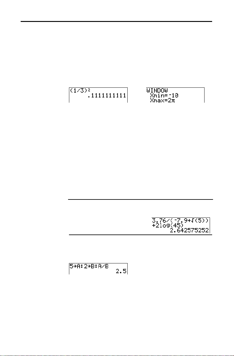
Calculate 3.76 ÷ (L7.9 + ‡5) + 2 log 45.
L, O, and G.
Ë
3
76 ¥ £ Ì 7 Ë 9
y
[‡] 5 ¤
Ã
2 « 45
Í
Multiple Entries on a Line
To enter two or more expressions or instructions on a line,
separate them with colons (
stored together in last entry (
1-6 Operating the TI-83
¤
¤
Ã
ƒ
ENTRY
:
[
]). All instructions are
; page 1.16).
Page 33

Entering a Number in Scientific Notation
Functions
To enter a number in scientific notation, follow these
steps.
1. Enter the part of the number that precedes the
exponent. This value can be an expression.
2. Press y [
EE
]. å is pasted to the cursor location.
3. If the exponent is negative, press Ì, and then enter the
exponent, which can be one or two digits.
When you enter a number in scientific notation, the TI.83
does not automatically display answers in scientific or
engineering notation. The mode settings (page 1.9) and the
size of the number determine the display format.
L
A function returns a value. For example,
÷,
, +,
‡
(
, and log(
are the functions in the example on page 1.6. In general, the
first letter of each function is lowercase on the TI.83. Most
functions take at least one argument, as indicated by an open
parenthesis (
requires one argument, sin(
( ) following the name. For example, sin(
value
).
Instructions
Interrupting a Calculation
An instruction initiates an action. For example,
ClrDraw is
an instruction that clears any drawn elements from a
graph. Instructions cannot be used in expressions. In
general, the first letter of each instruction name is
uppercase. Some instructions take more than one
argument, as indicated by an open parenthesis (
end of the name. For example,
arguments,
Circle(X,Y,
radius
Circle( requires three
).
( ) at the
To interrupt a calculation or graph in progress, which
would be indicated by the busy indicator, press É.
When you interrupt a calculation, the menu is displayed.
•
To return to the home screen, select
•
To go to the location of the interruption, select
1:Quit.
2:Goto.
When you interrupt a graph, a partial graph is displayed.
•
To return to the home screen, press
‘
or any
nongraphing key.
•
To restart graphing, press a graphing key or select a
graphing instruction.
Operating the TI-83 1-7
Page 34

g
g
g
(
TI-83 Edit Keys
Keystrokes Result
~
|
or
}
or
y |
y ~
Í
‘
{
y
[
y
ƒ
y
[
„
†
INS
A.LOCK
Moves the cursor within an expression; these keys repeat.
Moves the cursor from line to line within an expression that
occupies more than one line; these keys repeat.
On the top line of an expression on the home screen, } moves
the cursor to the beginning of the expression.
On the bottom line of an expression on the home screen,
moves the cursor to the end of the expression.
Moves the cursor to the beginning of an expression.
Moves the cursor to the end of an expression.
Evaluates an expression or executes an instruction.
On a line with text on the home screen, clears the current line.
On a blank line on the home screen, clears everythin
home screen.
In an editor, clears the expression or value where the cursor is
located; it does not store a zero.
Deletes a character at the cursor; this key repeats.
] Changes the cursor to __ ; inserts characters in front of the
underline cursor; to end insertion, press y [
~
, or †.
Chan
operation (an operation in yellow above a key and to the left); to
cancel
Chan
character (a character in green above a key and to the right) or
executes
ƒ
] Changes the cursor to Ø; sets alpha-lock; subsequent keystrokes
on an alpha key) paste alpha characters; to cancel alpha-lock,
ƒ
press
Pastes an
Seq
n
in
†
on the
INS
] or press |, },
es the cursor to Þ; the next keystroke performs a
, press y again.
2nd
2nd
es the cursor to Ø; the next keystroke pastes an alpha
(Chapters 10 and 11); to cancel
SOLVE
ƒ
, press
or press |, }, ~, or †.
; name prompts set alpha-lock automatically.
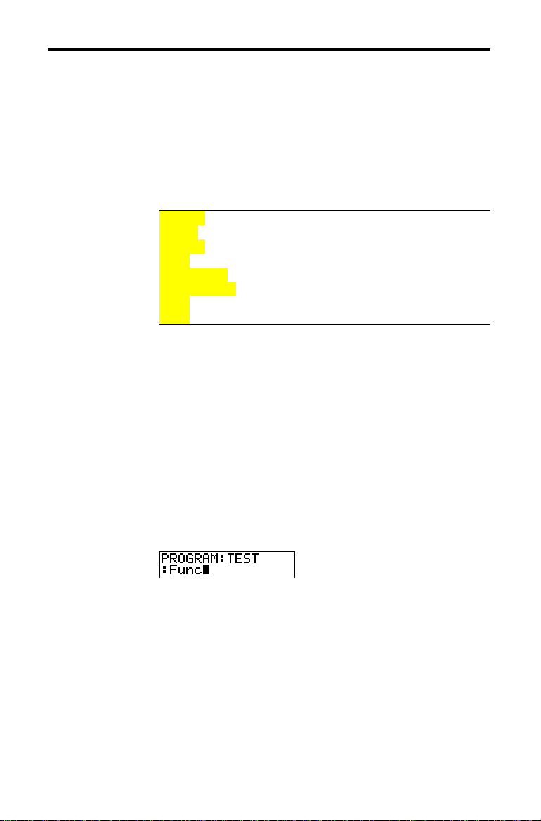
X
in
Func
mode, a T in
Par
mode, a q in
Pol
mode, or an
mode with one keystroke.
1-8 Operating the TI-83
Page 35
Setting Modes
Checking Mode Settings
Changing Mode Settings
Setting a Mode from a Program
Mode settings control how the TI.83 displays and
interprets numbers and graphs. Mode settings are retained
by the Constant Memory feature when the TI.83 is turned
off. All numbers, including elements of matrices and lists,
are displayed according to the current mode settings.
To display the mode settings, press
z
. The current
settings are highlighted. Defaults are highlighted below.
The following pages describe the mode settings in detail.
Normal Sci Eng
Float 0123456789
Radian Degree
Func Par Pol Seq
Connected Dot
Sequential Simul
Real a+bi re^qi
Full Horiz G-T
Numeric notation
Number of decimal places
Unit of angle measure
Type of graphing
Whether to connect graph points
Whether to plot simultaneously
Real, rectangular cplx, or polar cplx
Full screen, two split-screen modes
To change mode settings, follow these steps.
1. Press † or } to move the cursor to the line of the
setting that you want to change.
2. Press ~ or | to move the cursor to the setting you
want.
3. Press
Í
.
You can set a mode from a program by entering the name
of the mode as an instruction; for example,
Func or Float.
From a blank command line, select the mode setting from
the mode screen; the instruction is pasted to the cursor
location.
Operating the TI-83 1-9
Page 36

Normal, Sci, Eng
Notation modes only affect the way an answer is displayed
on the home screen. Numeric answers can be displayed
with up to 10 digits and a two-digit exponent. You can
enter a number in any format.
Normal notation mode is the usual way we express
numbers, with digits to the left and right of the decimal, as
in
12345.67.
Sci (scientific) notation mode expresses numbers in two
parts. The significant digits display with one digit to the left
of the decimal. The appropriate power of 10 displays to the
right of
Eng (engineering) notation mode is similar to scientific
E
, as in 1.234567
E
4.
notation. However, the number can have one, two, or three
digits before the decimal; and the power-of-10 exponent is
a multiple of three, as in
Note
: If you select
10 digits (or the absolute value is less than .001), the TI.83 expresses
the answer in scientific notation.
Normal
12.34567E3.
notation, but the answer cannot display in
Float, 0123456789
Float (floating) decimal mode displays up to 10 digits, plus
the sign and decimal.
0123456789 (fixed) decimal mode specifies the number of
digits (
Place the cursor on the desired number of decimal digits,
and then press
The decimal setting applies to
notation modes.
The decimal setting applies to these numbers:
•
An answer displayed on the home screen
•
Coordinates on a graph (Chapters 3, 4, 5, and 6)
•
The
and dy/dx values (Chapter 8)
•
Results of
and 6)
•
The regression equation stored after the execution of a
regression model (Chapter 12)
1-10 Operating the TI-83
0 through 9) to display to the right of the decimal.
Í
.
Normal, Sci, and Eng
Tangent(
CALCULATE
instruction equation of the line, x,
DRAW
operations (Chapters 3, 4, 5,
Page 37

Radian, Degree
Angle modes control how the TI.83 interprets angle values
in trigonometric functions and polar/rectangular
conversions.
Radian mode interprets angle values as radians. Answers
display in radians.
Degree mode interprets angle values as degrees. Answers
display in degrees.
Func, Par, Pol, Seq
Connected, Dot
Graphing modes define the graphing parameters. Chapters
3, 4, 5, and 6 describe these modes in detail.
Func (function) graphing mode plots functions, where Y is
a function of
Par (parametric) graphing mode plots relations, where X
X (Chapter 3).
and Y are functions of T (Chapter 4).
Pol (polar) graphing mode plots functions, where r is a
function of
Seq (sequence) graphing mode plots sequences (Chapter 6).
Connected plotting mode draws a line connecting each
q
(Chapter 5).
point calculated for the selected functions.
Dot plotting mode plots only the calculated points of the
selected functions.
Operating the TI-83 1-11
Page 38

Sequential, Simul
q
Real, a+bi, re^
i
Sequential graphing-order mode evaluates and plots one
function completely before the next function is evaluated
and plotted.
Simul (simultaneous) graphing-order mode evaluates and
plots all selected functions for a single value of
evaluates and plots them for the next value of
Note:
Regardless of which graphing mode is selected, the TI.83 will
sequentially graph all stat plots before it graphs any functions.
Real mode does not display complex results unless
X and then
X.
complex numbers are entered as input.
Two complex modes display complex results.
•
i
(rectangular complex mode) displays complex
a+b
numbers in the form a+bi.
q
•
i
(polar complex mode) displays complex numbers
re^
in the form re^
i
.
q
Full, Horiz, G.T
Full screen mode uses the entire screen to display a graph
or edit screen.
Each split-screen mode displays two screens
simultaneously.
•
Horiz (horizontal) mode displays the current graph on
the top half of the screen; it displays the home screen or
an editor on the bottom half (Chapter 9).
•
G.T (graph-table) mode displays the current graph on
the left half of the screen; it displays the table screen on
the right half (Chapter 9).
1-12 Operating the TI-83
Page 39

Using TI-83 Variable Names
Variables and Defined Items
On the TI.83 you can enter and use several types of data,
including real and complex numbers, matrices, lists,
functions, stat plots, graph databases, graph pictures, and
strings.
The TI.83 uses assigned names for variables and other
items saved in memory. For lists, you also can create your
own five-character names.
Variable Type Names
Real numbers
Complex numbers
Matrices
Lists
A, B
, . . . , Z,
A, B
, . . . , Z,
ãAä, ãBä, ãCä
L
L
1
2
,
q
q
ãJä
, . . . ,
L
L
L
3
,
,
L
4
5
6
,
,
, and user-
defined names
Y
Functions
Parametric equations
Polar functions
Sequence functions
Stat plots
Graph databases
Graph pictures
Strings
System variables
Y
1
,
X
1T
and
r
r
1
2
,
u, v, w
Plot1, Plot2, Plot3
GDB1, GDB2
Pic1, Pic2
Str1, Str2
Xmin, Xmax
2
, . . . ,
r
3
,
Y
9
Y
1T
, . . . ,
r
r
4
5
,
,
, . . . ,
, . . . ,
, . . . ,
, and others
Y
0
,
X
6T
r
6
,
GDB9, GDB0
Pic9, Pic0
Str9, Str0
and
Y
6T
Notes about Variables
•
You can create as many list names as memory will allow
(Chapter 11).
•
Programs have user-defined names and share memory
with variables (Chapter 16).
•
From the home screen or from a program, you can store
to matrices (Chapter 10), lists (Chapter 11), strings
Xmax
(Chapter 15), system variables such as
TblStart
1),
(Chapter 7), and all Y= functions (Chapters
(Chapter
3, 4, 5, and 6).
•
From an editor, you can store to matrices, lists, and
functions (Chapter 3).
Y=
•
From the home screen, a program, or an editor, you can
store a value to a matrix element or a list element.
•
You can use
DRAW STO
menu items to store and recall
graph databases and pictures (Chapter 8).
Operating the TI-83 1-13
Page 40
Storing Variable Values
Storing Values in a Variable
Displaying a Variable Value
Values are stored to and recalled from memory using
variable names. When an expression containing the name
of a variable is evaluated, the value of the variable at that
time is used.
To store a value to a variable from the home screen or a
program using the
follow these steps.
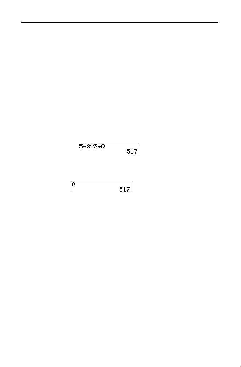
1. Enter the value you want to store. The value can be an
expression.
2. Press
3. Press
4. Press
To display the value of a variable, enter the name on a
blank line on the home screen, and then press
¿. !
ƒ
you want to store the value.
Í
evaluated. The value is stored to the variable.
¿
key, begin on a blank line and
is copied to the cursor location.
and then the letter of the variable to which
. If you entered an expression, it is
Í
.
1-14 Operating the TI-83
Page 41
Recalling Variable Values
Using Recall (RCL)
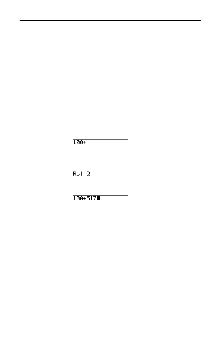
To recall and copy variable contents to the current cursor
location, follow these steps. To leave
RCLä
ã
.
1. Press y
Rcl and the edit cursor are displayed on
RCL
, press
‘
.
the bottom line of the screen.
2. Enter the name of the variable in any of five ways.
•
•
ƒ
Press
Press y
and then the letter of the variable.
LISTä
ã
, and then select the name of the list,
or press y [Ln].
•
•
Press
Press
display the
, and then select the name of the matrix.
to display the
VARS Y.VARS
menu or
VARS
menu; then select the type
~
and then the name of the variable or function.
•
Press
|
, and then select the name of the
program (in the program editor only).
The variable name you selected is displayed on the
bottom line and the cursor disappears.
3. Press
Í
. The variable contents are inserted where
the cursor was located before you began these steps.
to
Note:
You can edit the characters pasted to the expression without
affecting the value in memory.
Operating the TI-83 1-15
Page 42

ENTRY (Last Entry) Storage Area
Using ENTRY (Last Entry)
Accessing a Previous Entry
When you press
Í
on the home screen to evaluate an
expression or execute an instruction, the expression or
instruction is placed in a storage area called
entry). When you turn off the TI.83,
ENTRY
is retained in
ENTRY
(last
memory.
To recall
ENTRY
, press y [
ENTRY
]. The last entry is
pasted to the current cursor location, where you can edit
and execute it. On the home screen or in an editor, the
current line is cleared and the last entry is pasted to the
line.
Because the TI.83 updates
Í
, you can recall the previous entry even if you have
only when you press
ENTRY
begun to enter the next expression.
Ã
5
7
Í
ENTRY
y
[
]
The TI.83 retains as many previous entries as possible in
, up to a capacity of 128 bytes. To scroll those
ENTRY
entries, press y [
more than 128 bytes, it is retained for
be placed in the
¿ ƒ
1
A
ENTRY
ENTRY
] repeatedly. If a single entry is
, but it cannot
ENTRY
storage area.
Í
¿ ƒ
2
B
Í
ENTRY
y
[
]
If you press y [
entry, the newest stored entry is displayed again, then the
next-newest entry, and so on.
ENTRY
y
[
1-16 Operating the TI-83
ENTRY
] after displaying the oldest stored
]
Page 43
Reexecuting the Previous Entry
After you have pasted the last entry to the home screen
and edited it (if you chose to edit it), you can execute the
entry. To execute the last entry, press
To reexecute the displayed entry, press
Í
Í
.
again. Each
reexecution displays an answer on the right side of the
next line; the entry itself is not redisplayed.
¿ ƒ
0
N
Í
ƒ
ƒ
N
ã:ä
Ã
ƒ
¿ ƒ
1
¡ Í
N
N
Í
Í
Multiple Entry Values on a Line
Clearing ENTRY
To store to
two or more expressions or
ENTRY
instructions, separate each expression or instruction with
a colon, then press
separated by colons are stored in
When you press y [
Í
. All expressions and instructions
.
ENTRY
ENTRY
], all the expressions and
instructions separated by colons are pasted to the current
cursor location. You can edit any of the entries, and then
execute all of them when you press
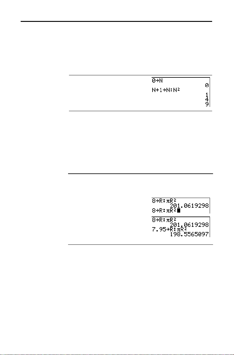
For the equation A=pr2, use trial and error to find the radius of a
circle that covers 200 square centimeters. Use 8 as your first
guess.
¿ ƒ
8
[:] y [p]
ENTRY
y
[
y |
y
7
R
ƒ
]
INS
[
ƒ
R ¡
] Ë 95
Í
Í
.
Í
Continue until the answer is as accurate as you want.
Clear Entries (Chapter 18) clears all data that the TI
holding in the
ENTRY
storage area.
.
83 is
Operating the TI-83 1-17
Page 44

Ans (Last Answer) Storage Area
Using Ans in an Expression
Continuing an Expression
When an expression is evaluated successfully from the
home screen or from a program, the TI.83 stores the
answer to a storage area called
Ans (last answer). Ans may
be a real or complex number, a list, a matrix, or a string.
When you turn off the TI.83, the value in
Ans is retained in
memory.
You can use the variable
most places. Press y [
Ans to represent the last answer in
ANS
] to copy the variable name Ans
to the cursor location. When the expression is evaluated, the
TI.83 uses the value of
Calculate the area of a garden plot 1.7 meters by 4.2 meters.
Then calculate the yield per square meter if the plot produces a
total of 147 tomatoes.
Ë
1
7 ¯ 4 Ë 2
Ans in the calculation.
Í
147
¥ y
[
ANS
]
Í
You can use Ans as the first entry in the next expression
without entering the value again or pressing y [
ANS
]. On
a blank line on the home screen, enter the function. The
TI.83 pastes the variable name
Ans to the screen, then the
function.
¥
5
2
Í
¯
Ë
9
9
Í
Storing Answers
To store an answer, store Ans to a variable before you
evaluate another expression.
Calculate the area of a circle of radius 5 meters. Next, calculate
the volume of a cylinder of radius 5 meters and height 3.3 meters,
and then store the result in the variable V.
p
y
[
] 5
Í
¯
3 Ë 3
Í
¿ ƒ
Í
1-18 Operating the TI-83
¡
V
Page 45

TI-83 Menus
Using a TI-83 Menu
Scrolling a Menu
You can access most TI.83 operations using menus. When
you press a key or key combination to display a menu, one
or more menu names appear on the top line of the screen.
•
The menu name on the left side of the top line is
highlighted. Up to seven items in that menu are
displayed, beginning with item
1, which also is
highlighted.
•
A number or letter identifies each menu item’s place in
the menu. The order is
and so on. The
menus only label items 1 through 9 and 0.
EDIT
•
When the menu continues beyond the displayed items, a
LIST NAMES, PRGM EXEC
1 through 9, then 0, then A, B, C,
, and
PRGM
down arrow ( $ ) replaces the colon next to the last
displayed item.
•
When a menu item ends in an ellipsis, the item displays
a secondary menu or editor when you select it.
To display any other menu listed on the top line, press
~
or | until that menu name is highlighted. The cursor
location within the initial menu is irrelevant. The menu is
displayed with the cursor on the first item.
Note:
The Menu Map in Appendix A shows each menu, each
operation under each menu, and the key or key combination you press
to display each menu.
To scroll down the menu items, press †. To scroll up the
menu items, press }.
To page down six menu items at a time, press
page up six menu items at a time, press
ƒ †
ƒ }
. To
. The
green arrows on the calculator, between † and }, are the
page-down and page-up symbols.
To wrap to the last menu item directly from the first menu
item, press }. To wrap to the first menu item directly from
the last menu item, press †.
Operating the TI-83 1-19
Page 46

Selecting an Item from a Menu
You can select an item from a menu in either of two ways.
•
Press the number or letter of the item you want to
select. The cursor can be anywhere on the menu, and
the item you select need not be displayed on the screen.
•
Press † or } to move the cursor to the item you want,
and then press
Í
.
After you select an item from a menu, the TI.83 typically
displays the previous screen.
Note:
On the
menus, only items 1 through 9 and 0 are labeled in such a way that
you can select them by pressing the appropriate number key. To move
the cursor to the first item beginning with any alpha character or q,
press the key combination for that alpha character or q. If no items
begin with that character, then the cursor moves beyond it to the next
item.
Calculate
LIST NAMES, PRGM EXEC
3
‡
27.
, and
PRGM EDIT
† † † Í
27
Í
¤
Leaving a Menu without Making a Selection
You can leave a menu without making a selection in any of
four ways.
•
Press y [
•
Press
•
Press a key or key combination for a different menu,
such as
•
Press a key or key combination for a different screen,
such as o or y [
QUIT
] to return to the home screen.
‘
to return to the previous screen.
or y [
LIST
TABLE
].
].
1-20 Operating the TI-83
Page 47

VARS and VARS Y-VARS Menus
VARS Menu
Selecting a Variable from the VARS Menu or VARS Y-VARS Menu
You can enter the names of functions and system variables
in an expression or store to them directly.
To display the
menu, press
VARS
. All
VARS
menu
items display secondary menus, which show the names of
the system variables.
1:Window, 2:Zoom, and 5:Statistics
each access more than one secondary menu.
VARS Y-VARS
1: Window
2: Zoom
3: GDB
4: Picture
5: Statistics
6: Table
7: String
To display the
1:Function, 2:Parametric, and 3:Polar display secondary
menus of the
VARS Y-VARS
1: Function
2: Parametric
3: Polar
4: On/Off
Note:
as the second functions of ¬, −, and ®.
...
...
...
...
...
...
...
VARS Y.VARS
function variables.
Y=
...
...
...
The sequence variables (
Y
X
...
n
r
Lets you select/deselect functions
To select a variable from the
q
, and
X/Y, T/
ZX/ZY, ZT/Z
Graph database
Picture
, G, EQ,
XY
TABLE
String
q
variables
TEST
variables
variables
menu, press
n
functions
T
T
n
n
, Y
functions
functions
u, v, w
) are located on the keyboard
VARS
variables
U/V/W
, and ZU variables
variables
, and
PTS
variables
~
or
VARS Y.VARS
.
menu,
follow these steps.
1. Display the
•
•
Press
Press
~
2. Select the type of variable, such as
menu or 3:Polar from the
VARS
or
VARS
VARS Y.VARS
to display the
to display the
menu.
menu.
VARS
VARS Y.VARS
2:Zoom from the
VARS Y.VARS
menu.
menu. A
secondary menu is displayed.
3. If you selected
the
VARS
1:Window, 2:Zoom, or 5:Statistics from
menu, you can press ~ or | to display other
secondary menus.
4. Select a variable name from the menu. It is pasted to the
cursor location.
Operating the TI-83 1-21
Page 48

Equation Operating System (EOS™)
Order of Evaluation
The Equation Operating System (EOSé) defines the order
in which functions in expressions are entered and
evaluated on the TI.83. EOS lets you enter numbers and
functions in a simple, straightforward sequence.
EOS evaluates the functions in an expression in this order:
1 Single-argument functions that precede the
‡
argument, such as
2 Functions that are entered after the argument,
such as
1
2
M
,
, !, ¡, r, and conversions
3 Powers and roots, such as 2^5 or 5
(
, sin(, or log(
x
‡
32
4 Permutations (nPr) and combinations (nCr)
5 Multiplication, implied multiplication, and
division
6 Addition and subtraction
7 Relational functions, such as > or
8 Logic operator and
9 Logic operators or and xor
Within a priority level, EOS evaluates functions from left to
right.
Calculations within parentheses are evaluated first.
Multiargument functions, such as
nDeriv(A2,A,6), are
evaluated as they are encountered.
1-22 Operating the TI-83
Page 49

Implied Multiplication
The TI.83 recognizes implied multiplication, so you need
not press ¯ to express multiplication in all cases. For
example, the TI.83 interprets
p
2
, 4sin(46), 5(1+2), and (2
as implied multiplication.
Note:
TI.83 implied multiplication rules differ from those of the TI.82.
For example, the TI.83 evaluates
evaluates
1à2X
as
1/(2äX)
1à2X
(Chapter 2).
as
(1à2)äX
, while the TI.82
ä
5)7
Parentheses
Negation
All calculations inside a pair of parentheses are completed
first. For example, in the expression
evaluates the portion inside the parentheses,
multiplies the answer,
3, by 4.
4(1+2), EOS first
1+2, and then
You can omit the close parenthesis ( ) ) at the end of an
expression. All open parenthetical elements are closed
automatically at the end of an expression. This is also true
for open parenthetical elements that precede the store or
display-conversion instructions.
Note:
An open parenthesis following a list name, matrix name, or
function name does not indicate implied multiplication. It specifies
elements in the list (Chapter 11) or matrix (Chapter 10) and specifies a
value for which to solve the
function.
Y=
To enter a negative number, use the negation key. Press
Y=
Ì
and then enter the number. On the TI.83, negation is in the
third level in the EOS hierarchy. Functions in the first
level, such as squaring, are evaluated before negation.
2
M
X
For example,
, evaluates to a negative number (or 0).
Use parentheses to square a negative number.
Note:
Use the ¹ key for subtraction and the Ì key for negation. If
you press ¹ to enter a negative number, as in
press Ì to indicate subtraction, as in
press
ä
A
(
M
B
ƒ
).
ƒ
A
Ì
B, it is interpreted as implied multiplication
9
9
¯ ¹ 7, or if you
Ì 7, an error occurs. If you
Operating the TI-83 1-23
Page 50

Error Conditions
Diagnosing an Error
Correcting an Error
The TI.83 detects errors while performing these tasks.
•
Evaluating an expression
•
Executing an instruction
•
Plotting a graph
•
Storing a value
When the TI.83 detects an error, it returns an error
message as a menu title, such as
ERR:DOMAIN
. Appendix B describes each error type and
ERR:SYNTAX
or
possible reasons for the error.
•
If you select
1:Quit (or press
y
[
QUIT
] or
‘
), then
the home screen is displayed.
•
If you select
2:Goto, then the previous screen is
displayed with the cursor at or near the error location.
Note
: If a syntax error occurs in the contents of a Y= function during
program execution, then the
to the program.
Goto
option returns to the Y= editor, not
To correct an error, follow these steps.
1. Note the error type (
2. Select
2:Goto, if it is available. The previous screen is
ERR:
error type
).
displayed with the cursor at or near the error location.
3. Determine the error. If you cannot recognize the error,
refer to Appendix B.
4. Correct the expression.
1-24 Operating the TI-83
Page 51

Math, Angle, and Test
2
Contents
Operations
Getting Started: Coin Flip
Keyboard Math Operations
MATH
Operations
Using the Equation Solver
MATH NUM
Entering and Using Complex Numbers
MATH CPX
MATH PRB
ANGLE
TEST
TEST LOGIC
(Number) Operations
(Complex) Operations
(Probability) Operations
Operations
(Relational) Operations
(Boolean) Operations
................................
..............................
........................................
...............................
........................
.......................
.......................................
............................
......................
...................
.....................
2-2
2-3
2-5
2-8
2-13
2-16
2-18
2-20
2-23
2-24
2-26
Math, Angle, and Test Operations 2-1
Page 52
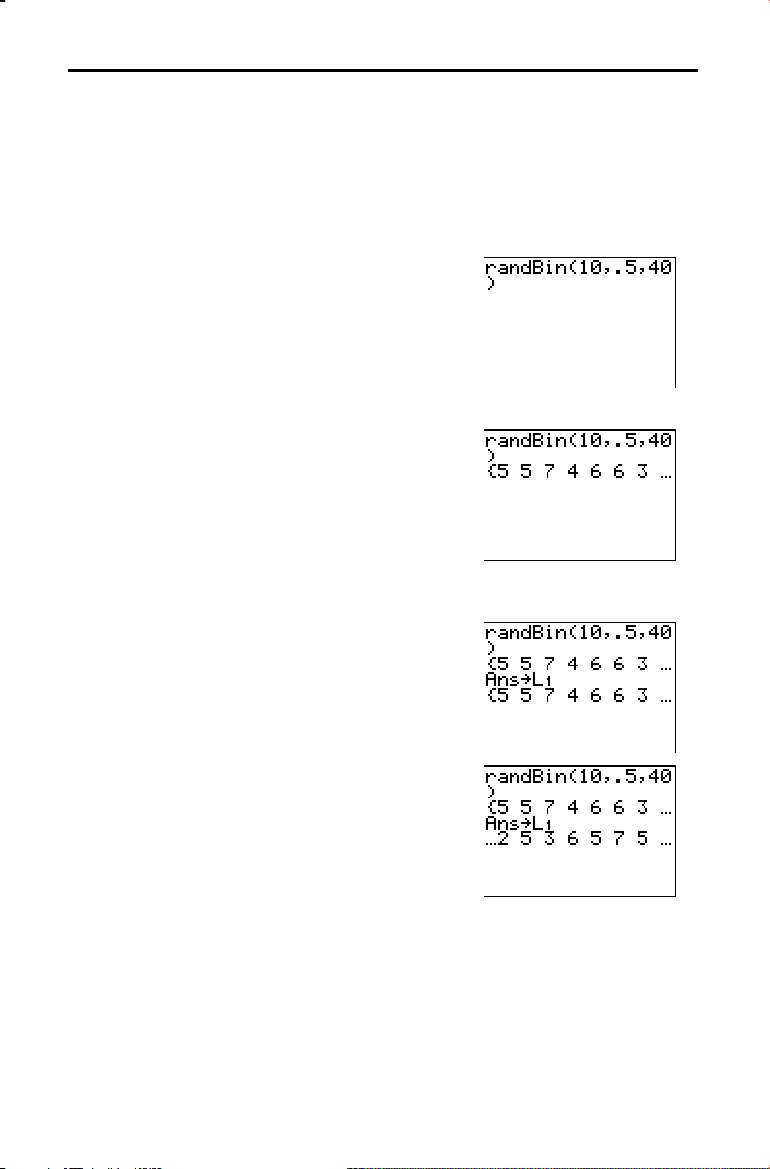
Getting Started: Coin Flip
Getting Started is a fast-paced introduction. Read the chapter for details.
Suppose you want to model flipping a fair coin 10 times. You want to track
how many of those 10 coin flips result in heads. You want to perform this
simulation 40 times. With a fair coin, the probability of a coin flip resulting in
heads is 0.5 and the probability of a coin flip resulting in tails is 0.5.
1. Begin on the home screen. Press
display the
select
randBin( is pasted to the home screen. Press
10 to enter the number of coin flips. Press
¢
. Press
MATH PRB
7:randBin( (random Binomial).
Ë
5 to enter the probability of
heads. Press ¢. Press
menu. Press 7 to
40 to enter the
|
to
number of simulations. Press ¤.
2. Press
Í
to evaluate the expression. A
list of 40 elements is displayed. The list
contains the count of heads resulting from
each set of 10 coin flips. The list has 40
elements because this simulation was
performed 40 times. In this example, the
coin came up heads five times in the first
set of 10 coin flips, five times in the second
set of 10 coin flips, and so on.
L1ä
ã
3. Press
¿ y
to the list name
Í
1
L
. You then can use the
to store the data
data for another activity, such as plotting a
histogram (Chapter 12).
4. Press ~ or | to view the additional counts
in the list. Ellipses (
...) indicate that the list
continues beyond the screen.
Note:
numbers, your list elements may differ from those
in the example.
Since
randBin(
generates random
2-2 Math, Angle, and Test Operations
Page 53

Keyboard Math Operations
Using Lists with Math Operations
+ (Addition),
N
(Subtraction),
ä
(Multiplication),
à
(Division)
Trigonometric Functions
Math operations that are valid for lists return a list
calculated element by element. If you use two lists in the
same expression, they must be the same length.
You can use + (addition, Ã), N (subtraction, ¹),
ä
(multiplication, ¯), and à (division, ¥) with real and
complex numbers, expressions, lists, and matrices. You
cannot use
valueA
valueA
à
with matrices.
valueB valueA
+
ä
valueB valueA
N
à
valueB
valueB
You can use the trigonometric (trig) functions (sine, ˜;
cosine, ™; and tangent, š) with real numbers,
expressions, and lists. The current angle mode setting
affects interpretation. For example,
L
returns
sin(
You can use the inverse trig functions (arcsine, y [
arccosine, y [
.9880316241
value
) cos(
; in Degree mode it returns .5.
value
L
1
COS
]; and arctangent, y [
sin(30) in Radian mode
) tan(
TAN
value
L
1
]) with
)
SIN
real numbers, expressions, and lists. The current angle
mode setting affects interpretation.
1
L
value
sin
(
) cos
Note:
The trig functions do not operate on complex numbers.
1
L
value
(
) tan
1
L
value
(
L
1
];
)
^ (Power),
2
(Square),
‡
( (Square Root)
1
L
(Inverse)
‡
You can use ^ (power, ›), 2 (square, ¡), and
root, y [
lists, and matrices. You cannot use
value
You can use
‡
]) with real and complex numbers, expressions,
‡
(
with matrices.
power value
^
1
L
(inverse,
2
—
) with real and complex
(
(square
value
‡
(
numbers, expressions, lists, and matrices. The
multiplicative inverse is equivalent to the reciprocal, 1
1
L
value
Math, Angle, and Test Operations 2-3
)
à
x
.
Page 54

log(, 10^(, ln(
e^( (Exponential)
You can use log( (logarithm, «), 10^( (power of 10,
x
10
]), and ln( (natural log, µ) with real or complex
[
numbers, expressions, and lists.
log(
e^(
a power. You can use
) 10^(
value
(exponential, y
)ln(
power
x
e
ã
]) returns the constant e raised to
e^( with real or complex numbers,
value
expressions, and lists.
e^(
power
)
y
)
e (Constant)
L
(Negation)
p
(Pi)
e (constant,
Press y [
calculations, the TI-83 uses 2.718281828459 for
M
(negation, Ì) returns the negative of
y
[e]) is stored as a constant on the TI-83.
e
] to copy e to the cursor location. In
value
e.
. You can use
with real or complex numbers, expressions, lists, and
matrices.
M
value
EOS rules (Chapter 1) determine when negation is
evaluated. For example,
because squaring is evaluated before negation. Use
parentheses to square a negated number, as in
Note:
On the TI-83, the negation symbol (
the subtraction sign (
p
(Pi, y [p]) is stored as a constant in the TI-83. In
N
), which is displayed when you press ¹.
calculations, the TI-83 uses 3.1415926535898 for
2
L
A
returns a negative number,
(LA)
M
) is shorter and higher than
2
p
.
M
.
2-4 Math, Angle, and Test Operations
Page 55
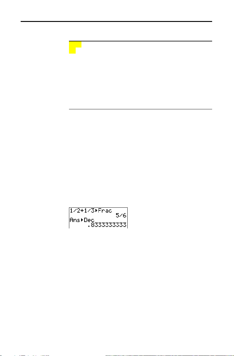
MATH Operations
MATH Menu
4
Frac,
4
Dec
MATH
To display the
MATH NUM CPX PRB
1:4Frac
2:4Dec
3
3:
3
‡
4:
(
x
‡
5:
6: fMin(
7: fMax(
8: nDeriv(
9: fnInt(
0: Solver
Frac
4
...
(display as a fraction) displays an answer as its
menu, press
Displays the answer as a fraction.
Displays the answer as a decimal.
Calculates the cube.
Calculates the cube root.
Calculates the
Finds the minimum of a function.
Finds the maximum of a function.
Computes the numerical derivative.
Computes the function integral.
Displays the equation solver.
rational equivalent. You can use
.
th
x
root.
Frac
4
with real or complex
numbers, expressions, lists, and matrices. If the answer
cannot be simplified or the resulting denominator is more
than three digits, the decimal equivalent is returned. You
Frac
Frac
4
4
following
Dec
4
can only use
value
Dec
4
(display as a decimal) displays an answer in decimal
form. You can use
expressions, lists, and matrices. You can only use
4
Dec
value
.
following
value
value
.
with real or complex numbers,
Dec
4
Math, Angle, and Test Operations 2-5
Page 56

3
(Cube),
3
‡
( (Cube Root)
3
(cube) returns the cube of
value
. You can use 3 with real
or complex numbers, expressions, lists, and square
matrices.
3
value
3
‡
(
(cube root) returns the cube root of
3
‡
(
with real or complex numbers, expressions, and lists.
3
value
‡
(
)
value
. You can use
x
‡
(Root)
fMin(, fMax(
x
th
x
‡
(
root) returns the
th
root
x
of
value
. You can use
x
‡
with real or complex numbers, expressions, and lists.
x
th
root
x
fMin( (function minimum) and fMax( (function maximum)
value
‡
return the value at which the local minimum or local
maximum value of
occurs, between
and fMax( are not valid in
controlled by
â
L
1
5).
expression,variable,lower,upper
fMin(
expression,variable,lower,upper
fMax(
Note:
In this guidebook, optional arguments and the commas that
accompany them are enclosed in brackets ([ ]).
expression
lower
tolerance
with respect to
upper
and
expression
values for
. The accuracy is
(if not specified, the default is
[
,
[
variable
tolerance
tolerance
,
variable
]
)
]
)
.
fMin(
2-6 Math, Angle, and Test Operations
Page 57

nDeriv(
nDeriv( (numerical derivative) returns an approximate
derivative of
value
at which to calculate the derivative and H (if not
specified, the default is 1
expression
with respect to
â
3). nDeriv( is valid only for real
L
variable
, given the
numbers.
expression,variable,value
nDeriv(
nDeriv( uses the symmetric difference quotient method,
H
[
]
,
)
which approximates the numerical derivative value as the
slope of the secant line through these points.
(
x
x
NH
x
f¢(
) =
f
+H)Nf(
)
H
2
As H becomes smaller, the approximation usually becomes
more accurate.
fnInt(
You can use nDeriv( once in
method used to calculate
expression
nDeriv(, the TI
. Because of the
-
83 can return a
false derivative value at a nondifferentiable point.
fnInt( (function integral) returns the numerical integral
limit,
expression
upper
â
5). fnInt( is valid only for real
L
with respect to
limit, and a
tolerance
(Gauss-Kronrod method) of
variable
, given
lower
not specified, the default is 1
numbers.
expression,variable,lower,upper
fnInt(
To speed the drawing of integration graphs (when
Tip:
in a Y= equation), increase the value of the
before you press
s
.
tolerance
[
,
window variable
Xres
]
)
fnInt(
is used
Math, Angle, and Test Operations 2-7
(if
Page 58
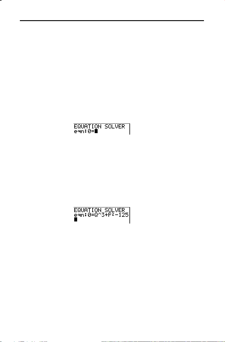
Using the Equation Solver
Solver
Entering an Expression in the Equation Solver
Solver displays the equation solver, in which you can solve
for any variable in an equation. The equation is assumed to
be equal to zero.
When you select
•
The equation editor (see step 1 picture below) is
displayed when the equation variable
•
The interactive solver editor (see step 3 picture on page
2.9) is displayed when an equation is stored in
Solver is valid only for real numbers.
Solver, one of two screens is displayed.
eqn is empty.
eqn.
To enter an expression in the equation solver, assuming
that the variable
1. Select
eqn is empty, follow these steps.
0:Solver from the
MATH
menu to display the
equation editor.
2. Enter the expression in any of three ways.
•
Enter the expression directly into the equation
solver.
•
Paste a
variable name from the
Y=
VARS Y.VARS
menu to the equation solver.
•
Press y [
VARS Y.VARS
RCL
], paste a Y= variable name from the
menu, and press
Í
. The
expression is pasted to the equation solver.
The expression is stored to the variable
eqn as you
enter it.
2-8 Math, Angle, and Test Operations
Page 59
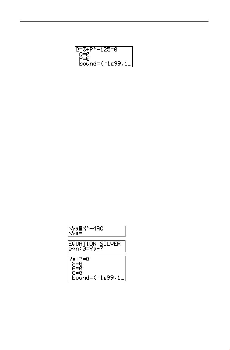
3. Press
displayed.
Í
or †. The interactive solver editor is
Entering and Editing Variable Values
•
The equation stored in
eqn is set equal to zero and
displayed on the top line.
•
Variables in the equation are listed in the order in
which they appear in the equation. Any values stored
to the listed variables also are displayed.
•
The default lower and upper bounds appear in the
last line of the editor (
•
$
is displayed in the first column of the bottom line
A
bound={L1å99,1å99}).
if the editor continues beyond the screen.
2
To use the solver to solve an equation such as
Tip:
eqn:0=KN.5MV
2
in the equation editor.
K=.5MV
, enter
When you enter or edit a value for a variable in the
interactive solver editor, the new value is stored in
memory to that variable.
You can enter an expression for a variable value. It is
evaluated when you move to the next variable.
Expressions must resolve to real numbers at each step
during the iteration.
You can store equations to any
such as
1
Y
or r6, and then reference the variables in the
VARS Y.VARS
variables,
equation. The interactive solver editor displays all
variables of all
functions referenced in the equation.
Y=
Math, Angle, and Test Operations 2-9
Page 60

Solving for a Variable in the Equation Solver
To solve for a variable using the equation solver after an
equation has been stored to
1. Select
0:Solver from the
eqn, follow these steps.
menu to display the
MATH
interactive solver editor, if not already displayed.
2. Enter or edit the value of each known variable. All
variables, except the unknown variable, must contain a
value. To move the cursor to the next variable, press
Í
or †.
3. Enter an initial guess for the variable for which you are
solving. This is optional, but it may help find the
solution more quickly. Also, for equations with multiple
roots, the TI-83 will attempt to display the solution that
is closest to your guess.
upper + lower
The default guess is calculated as
(
)
2
.
2-10 Math, Angle, and Test Operations
Page 61

4. Edit
bound={
lower,upper
}.
lower
and
upper
are the
bounds between which the TI-83 searches for a solution.
This is optional, but it may help find the solution more
quickly. The default is
bound={L1å99,1å99}.
5. Move the cursor to the variable for which you want to
solve and press
•
The solution is displayed next to the variable for
ƒ
SOLVE
[
] (above the
Í
key).
which you solved. A solid square in the first column
marks the variable for which you solved and
indicates that the equation is balanced. An ellipsis
shows that the value continues beyond the screen.
Note:
When a number continues beyond the screen, be sure to
press ~ to scroll to the end of the number to see whether it
ends with a negative or positive exponent. A very small number
may appear to be a large number until you scroll right to see
the exponent.
•
The values of the variables are updated in memory.
•
diff
leftNrt=
diff
is displayed in the last line of the editor.
is the difference between the left and right sides
of the equation. A solid square in the first column
next to
leftNrt= indicates that the equation has been
evaluated at the new value of the variable for which
you solved.
Math, Angle, and Test Operations 2-11
Page 62
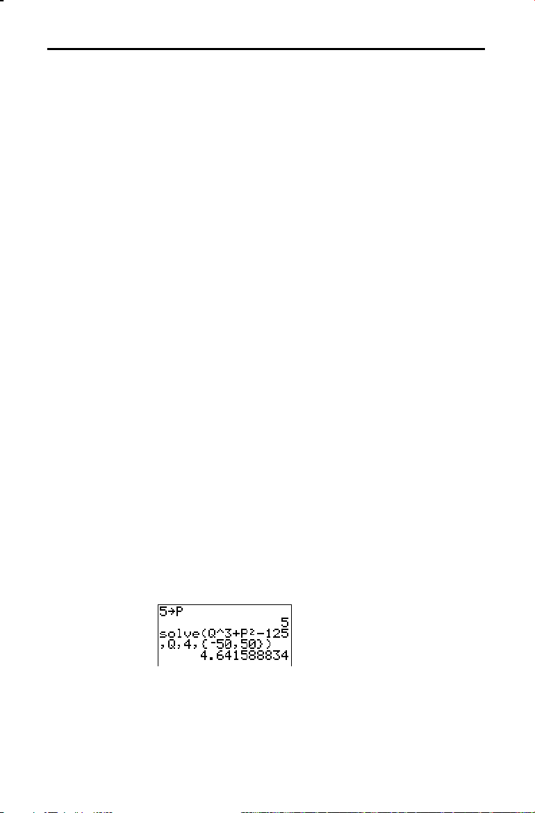
Editing an Equation Stored to eqn
To edit or replace an equation stored to eqn when the
interactive equation solver is displayed, press } until the
equation editor is displayed. Then edit the equation.
Equations with Multiple Roots
Further Solutions
Controlling the Solution for Solver or solve(
Using solve( on the Home Screen or from a Program
Some equations have more than one solution. You can
enter a new initial guess (page 2.10) or new bounds
(page 2.11) to look for additional solutions.
After you solve for a variable, you can continue to explore
solutions from the interactive solver editor. Edit the values
of one or more variables. When you edit any variable value,
the solid squares next to the previous solution and
diff
leftNrt=
which you now want to solve and press
disappear. Move the cursor to the variable for
ƒ
SOLVE
[
].
The TI-83 solves equations through an iterative process. To
control that process, enter bounds that are relatively close
to the solution and enter an initial guess within those
bounds. This will help to find a solution more quickly. Also,
it will define which solution you want for equations with
multiple solutions.
The function
solve( is available only from
CATALOG
or
from within a program. It returns a solution (root) of
expression
upper
and
default for
solve( is valid only for real numbers.
expression,variable,guess
solve(
expression
will not be updated in memory.
for
variable
, given an initial
guess
, and
lower
bounds within which the solution is sought. The
lower
is L1â99. The default for
[
,{
is assumed equal to zero. The value of
guess
upper
is 1â99.
lower,upper
}])
may be a value or a
variable
list of two values. Values must be stored for every variable
expression
in
evaluated.
, except
lower
and
variable
upper
, before
must be entered in list format.
expression
is
2-12 Math, Angle, and Test Operations
Page 63
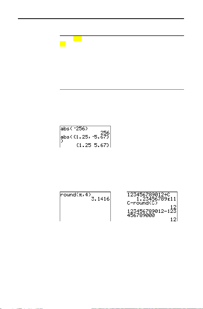
MATH NUM (Number) Operations
MATH NUM Menu
abs(
round(
To display the
MATH NUM CPX PRB
1: abs(
2: round(
3: iPart(
4: fPart(
5: int(
6: min(
7: max(
8: lcm(
9: gcd(
abs( (absolute value) returns the absolute value of real or
MATH NUM
menu, press
Absolute value
Round
Integer part
Fractional part
Greatest integer
Minimum value
Maximum value
Least common multiple
Greatest common divisor
~
.
complex (modulus) numbers, expressions, lists, and
matrices.
value
abs(
Note:
round( returns a number, expression, list, or matrix
rounded to
)
is also available on the
abs(
#decimals (
9). If
MATH CPX
#decimals
menu.
is omitted,
value
is rounded to the digits that are displayed, up to 10 digits.
value
#decimals
round(
[
,
]
)
Math, Angle, and Test Operations 2-13
Page 64
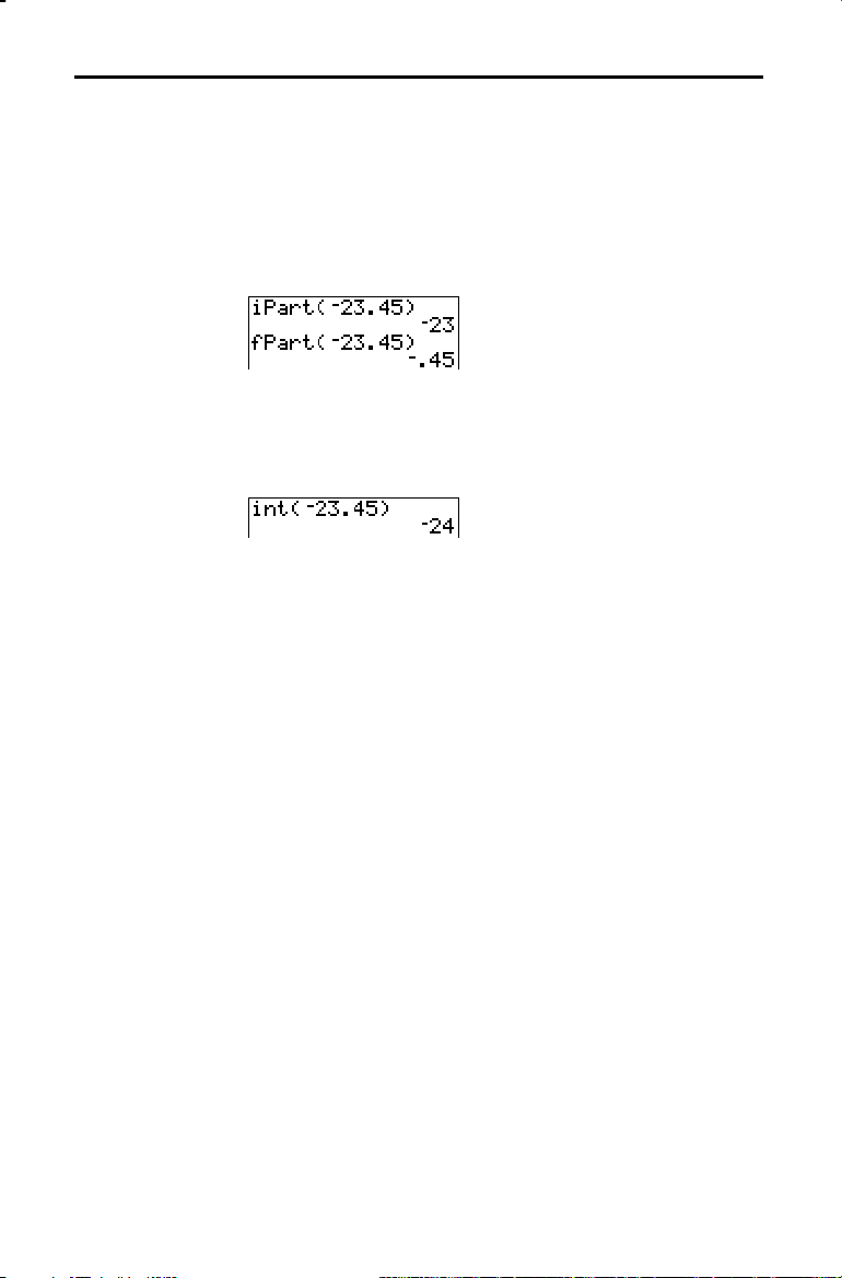
iPart(, fPart(
iPart( (integer part) returns the integer part or parts of real
or complex numbers, expressions, lists, and matrices.
value
iPart(
fPart( (fractional part) returns the fractional part or parts of
)
real or complex numbers, expressions, lists, and matrices.
value
fPart(
)
int(
int( (greatest integer) returns the largest integer
complex numbers, expressions, lists, and matrices.
value
int(
Note:
iPart(
less than the result of
)
value
For a given
for nonnegative numbers and negative integers, but one integer
, the result of
iPart(
int(
is the same as the result of
for negative noninteger numbers.
real or
2-14 Math, Angle, and Test Operations
Page 65

min(, max(
min( (minimum value) returns the smaller of
valueB
or the smallest element in
compared,
elements. If
each element in
max( (maximum value) returns the larger of
valueB
compared,
elements. If
each element in
min(
min(
min(
min(
min( returns a list of the smaller of each pair of
list
and
list
value
are compared,
value
with
or the largest element in
max( returns a list of the larger of each pair of
list
valueA,valueB
list
) max(
listA,listB
list,value
value
and
list
) max(
) max(
value
with
) max(
are compared,
list
. If
.
list
listA
. If
.
valueA,valueB
list
)
listA,listB
list,value
)
)
listA
min( compares
max( compares
)
valueA
and
valueA
and
listB
and
listB
and
are
are
lcm(, gcd(
and
min(
Note:
lcm( returns the least common multiple of
valueB
, both of which must be nonnegative integers. When
listA
and
listB
of each pair of elements. If
lcm( finds the lcm of each element in
gcd( returns the greatest common divisor of
valueB
, both of which must be nonnegative integers. When
listA
and
listB
of each pair of elements. If
gcd( finds the gcd of each element in
valueA,valueB
lcm(
listA,listB
lcm(
list,value
lcm(
also are available on the
max(
are specified,
lcm( returns a list of the lcm
list
are specified,
gcd( returns a list of the gcd
list
) gcd(
) gcd(
) gcd(
LIST MATH
value
and
and
are specified,
list
and
value
are specified,
list
and
valueA,valueB
listA,listB
list,value
)
valueA
)
and
value
valueA
value
)
menu.
.
and
.
Math, Angle, and Test Operations 2-15
Page 66
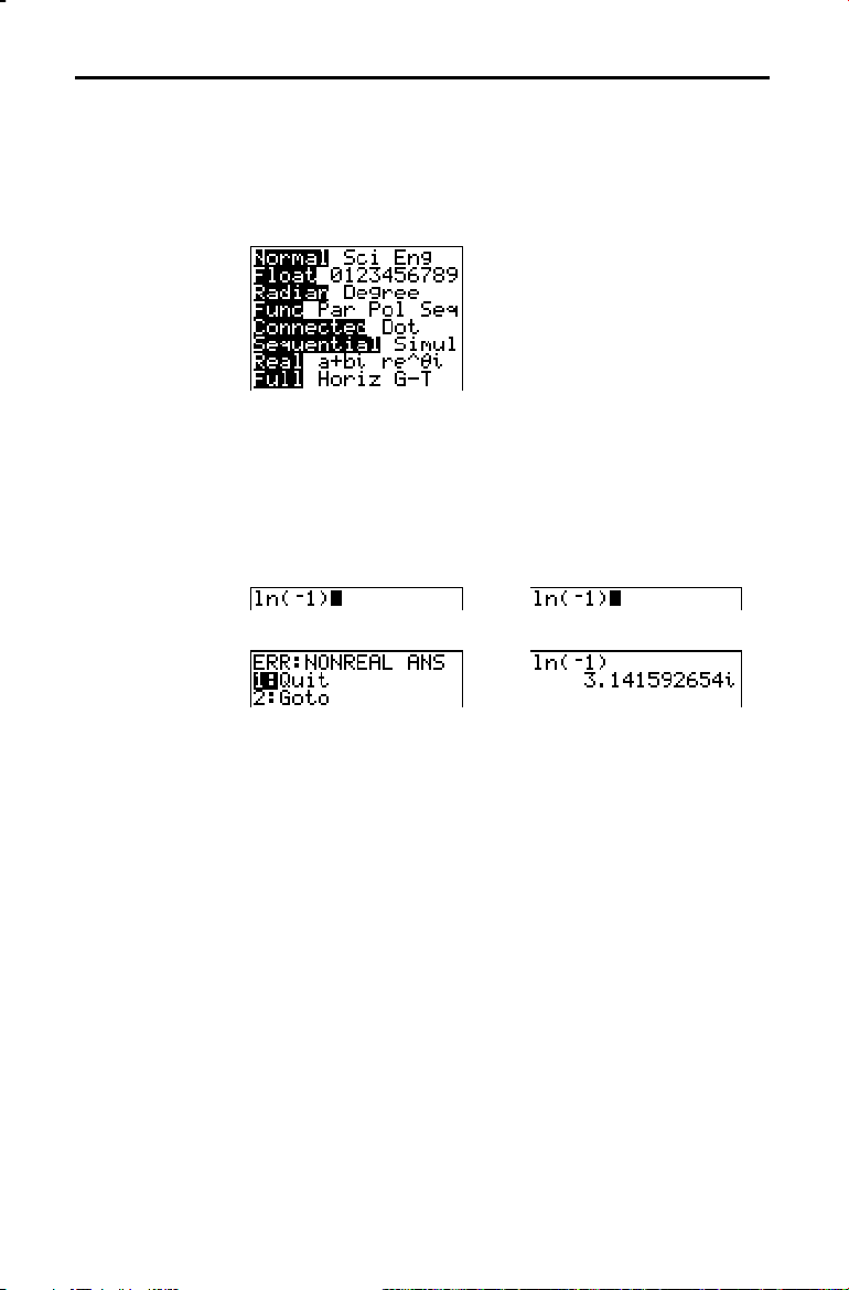
Entering and Using Complex Numbers
Complex-Number Modes
Entering Complex Numbers
The TI-83 displays complex numbers in rectangular form
and polar form. To select a complex-number mode, press
z
, and then select either of the two modes.
•
i
a+b
•
(rectangular-complex mode)
i
q
re^
(polar-complex mode)
On the TI-83, complex numbers can be stored to variables.
Also, complex numbers are valid list elements.
In
Real mode, complex-number results return an error,
unless you entered a complex number as input. For
example, in
ln(L1) returns an answer.
Real mode a+b
Real mode ln(L1) returns an error; in a+b
i
mode
i
mode
$$
Complex numbers are stored in rectangular form, but you
can enter a complex number in rectangular form or polar
form, regardless of the mode setting. The components of
complex numbers can be real numbers or expressions that
evaluate to real numbers; expressions are evaluated when
the command is executed.
Note about Radian versus Degree Mode
Radian mode is recommended for complex number
calculations. Internally, the TI-83 converts all entered trig
values to radians, but it does not convert values for
exponential, logarithmic, or hyperbolic functions.
In degree mode, complex identities such as
i
e
q
^(
) = cos(q) + i sin(q) are not generally true because
the values for cos and sin are converted to radians, while
those for e^() are not. For example,
e
^(i45) = cos(45) + i sin(45) is treated internally as
e
^(i45) = cos(p/4) + i sin(p/4). Complex identities are
always true in radian mode.
2-16 Math, Angle, and Test Operations
Page 67
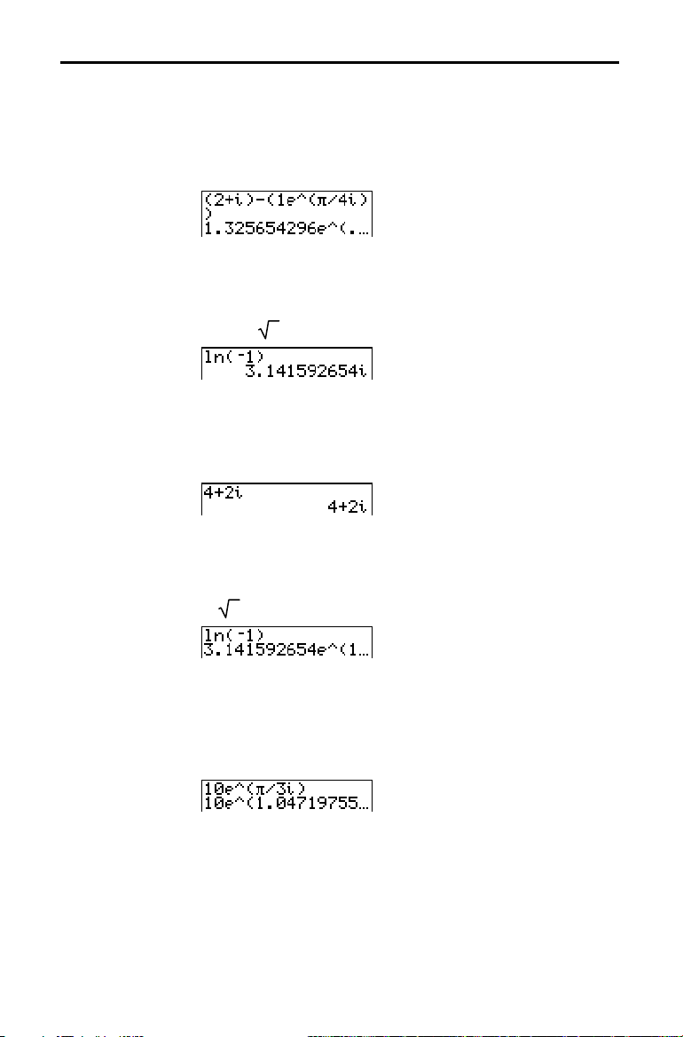
Interpreting Complex Results
Complex numbers in results, including list elements, are
displayed in either rectangular or polar form, as specified
by the mode setting or by a display conversion instruction
i
(page 2.19). In the example below,
re^
q
and
Radian modes
are set.
RectangularComplex Mode
Polar-Complex Mode
Rectangular-complex mode recognizes and displays a
complex number in the form
component,
equal to
b
is the imaginary component, and i is a constant
.
-1
a+b
, where
a
is the real
i
To enter a complex number in rectangular form, enter the
value of a (
of b (
real component
real component
imaginary component
imaginary componenti
N
(
+ or
)
), press à or ¹, enter the value
), and press y [i] (constant).
Polar-complex mode recognizes and displays a complex
i
q
number in the form
base of the natural log,
to
.
-1
To enter a complex number in polar form, enter the value
magnitude
of r (
enter the value of
re^
, where r is the magnitude, e is the
q
is the angle, and i is a constant equal
x
), press y [
q
angle
(
e
] (exponential function),
), press y [i] (constant), and
then press ¤.
i
magnitude
e^(
angle
)
Math, Angle, and Test Operations 2-17
Page 68

MATH CPX (Complex) Operations
MATH CPX Menu
conj(
real(
imag(
To display the
MATH NUM CPX PRB
1: conj(
2: real(
3: imag(
4: angle(
5: abs(
6:4Rect
7:4Polar
conj( (conjugate) returns the complex conjugate of a
MATH CPX
menu, press
Returns the complex conjugate.
Returns the real part.
Returns the imaginary part.
Returns the polar angle.
Returns the magnitude (modulus).
Displays the result in rectangular form.
Displays the result in polar form.
~ ~
.
complex number or list of complex numbers.
conj(a+
conj(re^(
real( (real part) returns the real part of a complex number
) returns
i
q
)) returns re^(
i
b
aNb
i
in a+b
Lq
i
mode.
i
) in re^
i
q
mode.
or list of complex numbers.
i
b
real(a+
real(re^(
imag( (imaginary part) returns the imaginary (nonreal) part
) returns
i
q
a
)) returns
.
ä
cos
q
r
(
).
of a complex number or list of complex numbers.
i
imag(a+
imag(re^(
b
) returns
i
q
b
)) returns
.
r
ä
sin(q)
.
2-18 Math, Angle, and Test Operations
Page 69

angle(
angle( returns the polar angle of a complex number or list
of complex numbers, calculated as tan
1
L
(b/a), where b is
the imaginary part and a is the real part. The calculation is
adjusted by +p in the second quadrant or Np in the third
quadrant.
1
L
(b/a)
angle(a+bi) returns
q
angle(re^(
i
)) returns
tan
q
.
, where Lp<q<p.
abs(
4
Rect
4
Polar
abs( (absolute value) returns the magnitude (modulus),
(real2+imag2)
, of a complex number or list of complex
numbers.
abs(a+bi) returns
q
abs(re^(
4
Rect
i
)) returns
(display as rectangular) displays a complex result in
(a2+b2)
r
.
(magnitude).
rectangular form. It is valid only at the end of an
expression. It is not valid if the result is real.
complex result
4
Polar
(display as polar) displays a complex result in polar
8
Rect
returns a+bi.
form. It is valid only at the end of an expression. It is not
valid if the result is real.
q
complex result
8
Polar
returns
i
r
e^(
).
Math, Angle, and Test Operations 2-19
Page 70
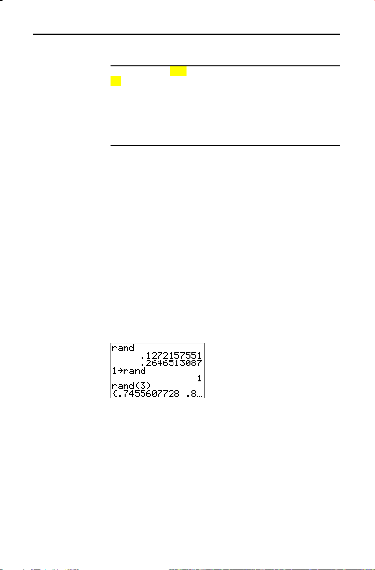
MATH PRB (Probability) Operations
MATH PRB Menu
rand
To display the
MATH NUM CPX PRB
1: rand
2: nPr
3: nCr
4: !
5: randInt(
6: randNorm(
7: randBin(
rand (random number) generates and returns one or more
MATH PRB
menu, press
Random-number generator
Number of permutations
Number of combinations
Factorial
Random-integer generator
Random # from Normal distribution
Random # from Binomial distribution
|
.
random numbers > 0 and < 1. To generate a list of randomnumbers, specify an integer > 1 for
trials). The default for
numtrials
rand[(
Tip:
To generate random numbers beyond the range of 0 to 1, you
can include
random number > 0 and < 5.
rand
in an expression. For example,
numtrials
)]
numtrials
is 1.
(number of
randä5
generates a
With each rand execution, the TI-83 generates the same
random-number sequence for a given seed value. The TI-83
factory-set seed value for
rand is 0. To generate a different
random-number sequence, store any nonzero seed value to
rand. To restore the factory-set seed value, store 0 to rand
or reset the defaults (Chapter 18).
Note:
The seed value also affects
randBin(
instructions (page 2.22).
randInt(, randNorm(
, and
2-20 Math, Angle, and Test Operations
Page 71
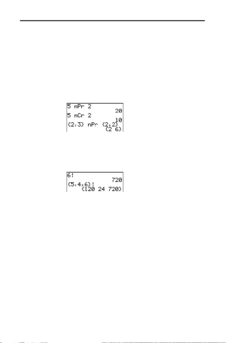
nPr, nCr
nPr (number of permutations) returns the number of
permutations of
number
number
items
nCr (number of combinations) returns the number of
must be nonnegative integers. Both
can be lists.
nPr
combinations of
number
number
items
must be nonnegative integers. Both
can be lists.
nCr
items
number
items
number
taken
taken
number
number
at a time.
items
at a time.
items
items
and
items
and
and
and
! (Factorial)
! (factorial) returns the factorial of either an integer or a
multiple of .5. For a list, it returns factorials for each
integer or multiple of .5.
value
!
The factorial is computed recursively using the relationship
Note:
(n+1)! = nän!, until n is reduced to either 0 or L1/2. At that point, the
definition 0!=1 or the definition (L1à2)!=‡p is used to complete the
calculation. Hence:
n!=nä(nN1)ä(nN2)ä ... ä2ä1, if n is an integer ‚0
n!= nä(nN1)ä(nN2)ä ... ä1à2
n! is an error, if neither n nor n+1à2 is an integer ‚0.
(The variable n equals
value
must be ‚L.5 and 69.
‡p
ä
, if n+1à2 is an integer ‚0
value
in the syntax description above.)
Math, Angle, and Test Operations 2-21
Page 72
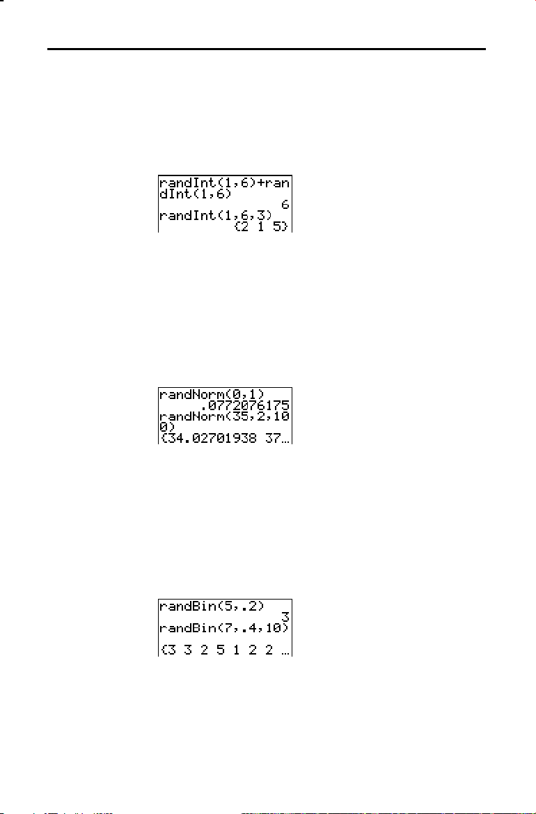
randInt(
randInt( (random integer) generates and displays a random
integer within a range specified by
lower
and
upper
integer
bounds. To generate a list of random numbers, specify an
integer >1 for
numtrials
(number of trials); if not
specified, the default is 1.
randInt(
lower,upper
numtrials
[
,
]
)
randNorm(
randBin(
randNorm( (random Normal) generates and displays a
random real number from a specified Normal distribution.
Each generated value could be any real number, but most
will be within the interval [mN3(s), m+3(s)]. To generate a
list of random numbers, specify an integer > 1 for
numtrials
(number of trials); if not specified, the default
is 1.
s
randNorm(m,
randBin( (random Binomial) generates and displays a
numtrials
[,
]
)
random integer from a specified Binomial distribution.
numtrials
(number of trials) must be ‚ 1.
prob
(probability
of success) must be ‚ 0 and 1. To generate a list of
random numbers, specify an integer > 1 for
numsimulations
(number of simulations); if not specified,
the default is 1.
randBin(
numtrials,prob
numsimulations
[
,
]
)
Note:
The seed value stored to
randNorm(
, and
randBin(
2-22 Math, Angle, and Test Operations
rand
instructions (page 2-20).
also affects
randInt(
,
Page 73

ANGLE Operations
ANGLE Menu
DMS Entry Notation
To display the
ANGLE
menu, press y [
ANGLE
]. The
ANGLE
menu displays angle indicators and instructions. The
Radian/Degree mode setting affects the TI
interpretation of
ANGLE
¡
1:
2: '
r
3:
4:8DMS
5: R8Pr(
6: R8Pq(
7: P8Rx(
8: P8Ry(
ANGLE
menu entries.
Degree notation
DMS minute notation
Radian notation
Displays as degree/minute/second
Returns r, given X and
Returns q, given X and
Returns x, given R and
Returns y, given R and
-
83’s
Y
Y
q
q
DMS (degrees/minutes/seconds) entry notation comprises
the degree symbol (
second symbol (
minutes
degrees
and
minutes'seconds
¡
¡
), the minute symbol ('), and the
degrees
").
seconds
must be a real number;
must be real numbers ‚ 0.
"
For example, enter for 30 degrees, 1 minute, 23 seconds. If
the angle mode is not set to
Degree, you must use
¡
so that
the TI-83 can interpret the argument as degrees, minutes,
and seconds.
Degree mode Radian mode
¡
(Degree)
¡
(degree) designates an angle or list of angles as degrees,
regardless of the current angle mode setting. In
Radian
mode, you can use ¡ to convert degrees to radians.
value
¡
value1,value2,value3,value4
{
¡
also designates
' (minutes) designates
" (seconds) designates
is not on the
"
Note:
degrees
(D) in DMS format.
minutes
seconds
menu. To enter ", press
ANGLE
,...,
value n
¡
}
(M) in DMS format.
(S) in DMS format.
ƒ
[ã].
Math, Angle, and Test Operations 2-23
Page 74
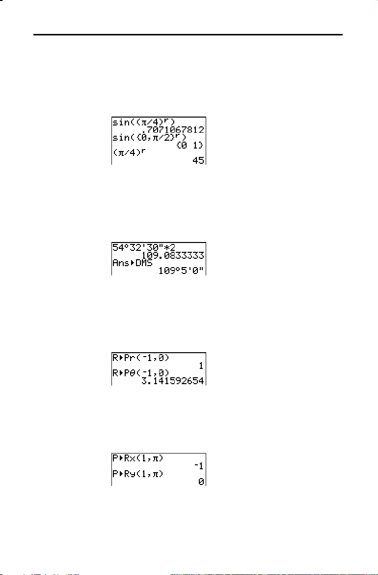
r
(Radians)
r
(radians) designates an angle or list of angles as radians,
regardless of the current angle mode setting. In
Degree
mode, you can use r to convert radians to degrees.
r
value
Degree mode
8
DMS
R8Pr(,
R8Pq(,
P8Rx(,
P8Ry(
8
DMS
(degree/minute/second) displays
format (page 2.23). The mode setting must be
answer
8
answer
R8Pr( converts rectangular coordinates to polar
coordinates and returns
to be interpreted as degrees, minutes, and seconds.
DMS
is valid only at the end of a line.
8
DMS
r. R8Pq( converts rectangular
coordinates to polar coordinates and returns
answer
in DMS
Degree for
q
. x and y can
be lists.
R8Pr(x,y), R8Pq(x,y)
Note: Radian
converts polar coordinates to rectangular
P8Rx(
coordinates and returns
x. P8Ry( converts polar
mode is set.
coordinates to rectangular coordinates and returns
q
can be lists.
P8Rx(r,q), P8Ry(r,q)
Note: Radian
mode is set.
y.
r
and
2-24 Math, Angle, and Test Operations
Page 75
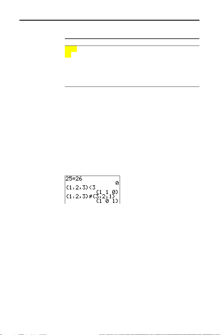
TEST (Relational) Operations
TEST Menu
=, ƒ,
>, ‚,
<,
TEST
To display the
This operator... Returns 1 (true) if...
TEST LOGIC
=
1:
ƒ
2:
>
3:
‚
4:
<
5:
6:
Relational operators compare
1
return
valueB
and ƒ only,
if the test is true or 0 if the test is false.
can be real numbers, expressions, or lists. For
valueA
complex numbers. If
menu, press y [
Equal
Not equal to
Greater than
Greater than or equal to
Less than
Less than or equal to
valueA
valueB
and
valueA
also can be matrices or
and
TEST
].
valueB
and
valueB
are matrices, both
and
valueA
and
=
must have the same dimensions.
Relational operators are often used in programs to control
program flow and in graphing to control the graph of a
function over specific values.
=
valueA
valueA
valueA
valueB valueAƒvalueB
>
valueB valueA‚valueB
<
valueB valueAvalueB
Using Tests
Relational operators are evaluated after mathematical
functions according to EOS rules (Chapter 1).
•
The expression
2+2=2+3
returns 0. The TI-83 performs
the addition first because of EOS rules, and then it
compares 4 to 5.
•
The expression
2+(2=2)+3
returns 6. The TI-83 performs
the relational test first because it is in parentheses, and
then it adds 2, 1, and 3.
Math, Angle, and Test Operations 2-25
Page 76

TEST LOGIC (Boolean) Operations
TEST LOGIC Menu
To display the
This operator... Returns a 1 (true) if...
TEST LOGIC
1: and
2: or
3: xor
4: not(
TEST LOGIC
menu, press y
Both values are nonzero (true).
At least one value is nonzero (true).
Only one value is zero (false).
The value is zero (false).
TESTä
ã
~.
Boolean Operators
and, or, xor
not(
Using Boolean Operations
Boolean operators are often used in programs to control
program flow and in graphing to control the graph of the
function over specific values. Values are interpreted as
zero (false) or nonzero (true).
and, or
expression is true or
to the table below.
, and
xor
(exclusive or) return a value of 1 if an
0
if an expression is false, according
valueA
and
valueB
can be real
numbers, expressions, or lists.
valueA
valueA
valueA
not(
not(
and
valueB
or
valueB
xor
valueB
valueA valueB and or xor
ƒ
0
ƒ
0 0 returns
0
ƒ
0 returns
ƒ
0 returns
0 0 returns
returns 1 if
value
value
(which can be an expression) is 0.
)
110
011
011
000
Boolean logic is often used with relational tests. In the
following program, the instructions store
4
into C.
2-26 Math, Angle, and Test Operations
Page 77
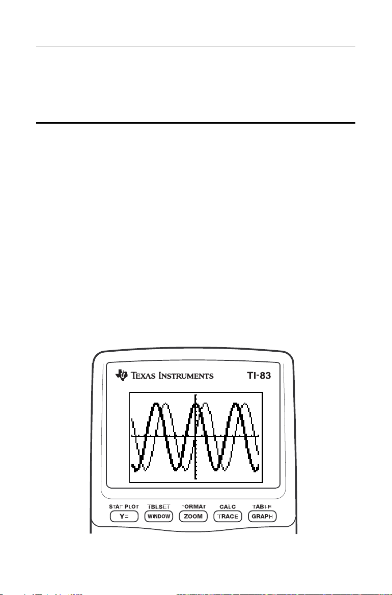
Function
g
3
Contents
Graphin
Getting Started: Graphing a Circle
Defining Graphs
Setting the Graph Modes
Defining Functions
Selecting and Deselecting Functions
Setting Graph Styles for Functions
Setting the Viewing Window Variables
Setting the Graph Format
Displaying Graphs
Exploring Graphs with the Free-Moving Cursor
Exploring Graphs with
Exploring Graphs with the
Using
ZOOM MEMORY
Using the
.........................................
.................................
......................................
................................
.......................................
TRACE
..................................
(Calculate) Operations
CALC
.......................
.....................
.......................
...................
...........................
Instructions
ZOOM
..................
..........
...........
3-2
3-3
3-4
3-5
3-7
3-9
3-11
3-13
3-15
3-17
3-18
3-20
3-23
3-25
Function Graphing 3-1
Page 78
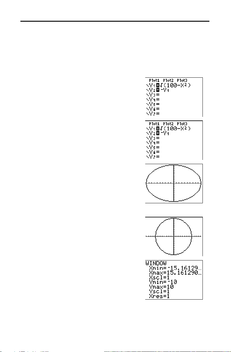
Getting Started: Graphing a Circle
Getting Started is a fast-paced introduction. Read the chapter for details.
Graph a circle of radius 10, centered on the origin in the standard viewing
window. To graph this circle, you must enter separate formulas for the upper
and lower portions of the circle. Then use
display and make the functions appear as a circle.
ZSquare (zoom square) to adjust the
Func mode, press
1. In
editor. Press y
Y=
Í
to enter the expression Y=‡(100NX
o
to display the
‡
ä
ã
¹ „ ¡ ¤
100
which defines the top half of the circle.
The expression Y=L‡(100NX
2
) defines the
bottom half of the circle. On the TI-83, you
can define one function in terms of another.
To define
negation sign. Press
VARS Y.VARS
select
1:Function. The
menu is displayed. Press
2. Press
q
1
Y2=LY
, press Ì to enter the
~
menu. Then press
to display the
FUNCTION
1 to select 1:Y
Í
secondary
6 to select 6:ZStandard. This is a
quick way to reset the window variables to
the standard values. It also graphs the
functions; you do not need to press
s
Notice that the functions appear as an
ellipse in the standard viewing window.
3. To adjust the display so that each pixel
represents an equal width and height, press
q
5 to select 5:ZSquare. The functions
are replotted and now appear as a circle on
the display.
to
1
2
),
.
.
4. To see the ZSquare window variables, press
p
and notice the new values for
Xmax, Ymin, and Ymax.
Xmin,
3-2 Function Graphing
Page 79

Defining Graphs
TI-83—Graphing Mode Similarities
Defining a Graph
Displaying and Exploring a Graph
Saving a Graph for Later Use
Chapter 3 specifically describes function graphing, but the
steps shown here are similar for each TI-83 graphing
mode. Chapters 4, 5, and 6 describe aspects that are unique
to parametric graphing, polar graphing, and sequence
graphing.
To define a graph in any graphing mode, follow these
steps. Some steps are not always necessary.
1. Press
z
and set the appropriate graph mode
(page 3.4).
2. Press o and enter, edit, or select one or more functions
in the
editor (page 3.5 and 3.7).
Y=
3. Deselect stat plots, if necessary (page 3.7).
4. Set the graph style for each function (page 3.9).
5. Press
p
and define the viewing window variables
(page 3.11).
FORMAT
6. Press y [
] and select the graph format settings
(page 3.13).
After you have defined a graph, press
s
to display it.
Explore the behavior of the function or functions using the
TI-83 tools described in this chapter.
You can store the elements that define the current graph to
any of 10 graph database variables (
and
GDB0; Chapter 8). To recreate the current graph later,
GDB1 through GDB9,
simply recall the graph database to which you stored the
original graph.
These types of information are stored in a
•
functions
Y=
•
Graph style settings
•
Window settings
•
Format settings
GDB.
You can store a picture of the current graph display to any
of 10 graph picture variables (
Pic1 through Pic9, and Pic0;
Chapter 8). Then you can superimpose one or more stored
pictures onto the current graph.
Function Graphing 3-3
Page 80

Setting the Graph Modes
Checking and Changing the Graphing Mode
To display the mode screen, press
z
. The default
settings are highlighted below. To graph functions, you
must select
Func mode before you enter values for the
window variables and before you enter the functions.
The TI-83 has four graphing modes.
•
Func (function graphing)
•
Par (parametric graphing; Chapter 4)
•
Pol (polar graphing; Chapter 5)
•
Seq (sequence graphing; Chapter 6)
Other mode settings affect graphing results. Chapter 1
describes each mode setting.
•
Float or 0123456789 (fixed) decimal mode affects
displayed graph coordinates.
•
Radian or Degree angle mode affects interpretation of
some functions.
•
Connected or Dot plotting mode affects plotting of
selected functions.
•
Sequential or Simul graphing-order mode affects
function plotting when more than one function is
selected.
Setting Modes from a Program
To set the graphing mode and other modes from a
program, begin on a blank line in the program editor and
follow these steps.
1. Press
2. Press †, ~, |, and } to place the cursor on the mode
that you want to select.
3. Press
location.
The mode is changed when the program is executed.
3-4 Function Graphing
z
to display the mode settings.
Í
to paste the mode name to the cursor
Page 81
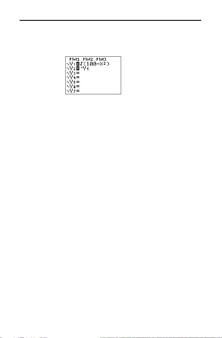
Defining Functions
Displaying Functions in the Y= Editor
Defining or Editing a Function
To display the Y= editor, press o. You can store up to 10
functions to the function variables
1
Y
through Y9, and Y0.
You can graph one or more defined functions at once. In
this example, functions
1
Y
and Y2 are defined and selected.
To define or edit a function, follow these steps.
1. Press o to display the
Y=
editor.
2. Press † to move the cursor to the function you want to
define or edit. To erase a function, press
‘
.
3. Enter or edit the expression to define the function.
•
You may use functions and variables (including
matrices and lists) in the expression. When the
expression evaluates to a nonreal number, the value
is not plotted; no error is returned.
•
The independent variable in the function is
mode defines
or press
•
When you enter the first character, the
ƒ
„
as X. To enter X, press
[X].
X. Func
„
= is
highlighted, indicating that the function is selected.
As you enter the expression, it is stored to the variable
n
Y
as a user-defined function in the Y= editor.
4. Press
Í
or † to move the cursor to the next
function.
Function Graphing 3-5
Page 82

Defining a Function from the Home Screen or a Program
To define a function from the home screen or a program,
begin on a blank line and follow these steps.
ã
[
] again.
ã
[
], enter the expression, and then press
.
1 to select 1:Function from the
menu.
1. Press
ƒ
2. Press
3. Press
VARS Y.VARS
ƒ
¿
~
4. Select the function name, which pastes the name to the
cursor location on the home screen or program editor.
5. Press
Í
to complete the instruction.
Evaluating Y= Functions in Expressions
expression
"
"!Y
n
When the instruction is executed, the TI-83 stores the
n
expression to the designated variable
function, and displays the message
You can calculate the value of a
value
value
)
of
X. A list of
specified
Yn(
n({value1,value2,value3, . . .,value n
Y
Y=
values
, selects the
Y
Done.
function Y
n
returns a list.
})
at a
3-6 Function Graphing
Page 83
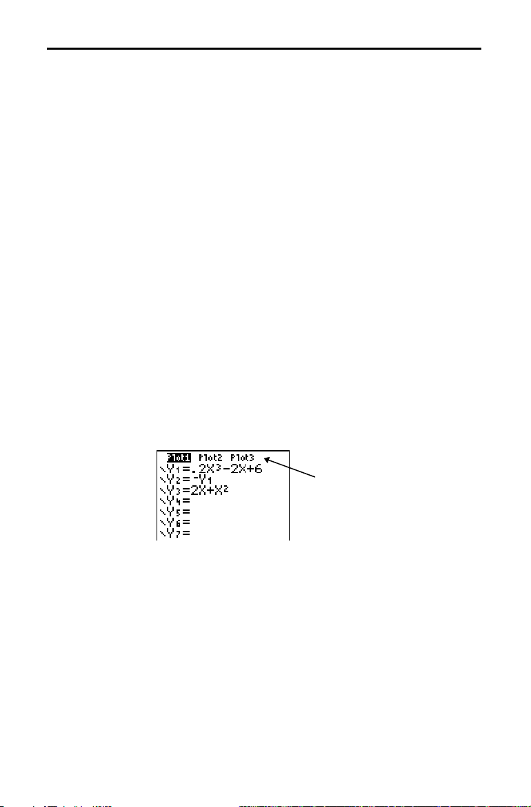
Selecting and Deselecting Functions
Selecting and Deselecting a Function
Turning On or Turning Off a Stat Plot in the Y= Editor
You can select and deselect (turn on and turn off) a
function in the
editor. A function is selected when the =
Y=
sign is highlighted. The TI-83 graphs only the selected
functions. You can select any or all functions
9
Y
, and Y0.
To select or deselect a function in the
Y=
1
Y
through
editor, follow
these steps.
1. Press o to display the
Y=
editor.
2. Move the cursor to the function you want to select or
deselect.
3. Press | to place the cursor on the function’s
4. Press
Í
to change the selection status.
= sign.
When you enter or edit a function, it is selected
automatically. When you clear a function, it is deselected.
To view and change the on/off status of a stat plot in the
editor, use Plot1 Plot2 Plot3 (the top line of the
Y=
editor). When a plot is on, its name is highlighted on this
Y=
line.
To change the on/off status of a stat plot from the
editor, press } and ~ to place the cursor on Plot1,
Y=
Plot2, or Plot3, and then press
Í
Plot1
Plot2
.
is turned on.
and
Plot3
are turned off.
Function Graphing 3-7
Page 84

Selecting and Deselecting Functions from the Home Screen or a Program
To select or deselect a function from the home screen or a
program, begin on a blank line and follow these steps.
1. Press
2. Select
3. Select
~
4:On/Off to display the
1:FnOn to turn on one or more functions or
2:FnOff to turn off one or more functions. The
to display the
VARS Y.VARS
ON/OFF
secondary menu.
menu.
instruction you select is copied to the cursor location.
4. Enter the number (
n
) of each function you want to turn on or turn off.
Y
•
If you enter two or more numbers, separate them
1 through 9, or 0; not the variable
with commas.
•
To turn on or turn off all functions, do not enter a
number after
function#
FnOn[
function#
FnOff[
5. Press
Í
FnOn or FnOff.
function#
,
function#
,
, . . .,
, . . .,
function n
function n
]
]
. When the instruction is executed, the
status of each function in the current mode is set and
Done is displayed.
For example, in
functions in the
Func mode, FnOff :FnOn 1,3 turns off all
editor, and then turns on Y1 and Y3.
Y=
3-8 Function Graphing
Page 85

g
g
Setting Graph Styles for Functions
Graph Style Icons in the Y= Editor
Setting the Graph Style
This table describes the graph styles available for function
graphing. Use the styles to visually differentiate functions
to be graphed together. For example, you can set
solid line,
Icon Style Description
ç
è
é
ê
ë
2
Y
as a dotted line, and Y3 as a thick line.
Line A solid line connects plotted points; this is
the default in
Connected mode
Thick A thick solid line connects plotted points
Above Shading covers the area a*bove the graph
Below Shading covers the area below the graph
Path A circular cursor traces the leadin
1
Y
as a
edge of
the graph and draws a path
ì
Animate A circular cursor traces the leadin
edge of
the graph without drawing a path
í
Dot A small dot represents each plotted point;
Note:
Some graph styles are not available in all graphing modes.
Chapters 4, 5, and 6 list the styles for
this is the default in
Par, Pol
Dot mode
, and
Seq
modes.
To set the graph style for a function, follow these steps.
1. Press o to display the
Y=
editor.
2. Press † and } to move the cursor to the function.
3. Press | | to move the cursor left, past the
= sign, to
the graph style icon in the first column. The insert
cursor is displayed. (Steps 2 and 3 are interchangeable.)
4. Press
Í
repeatedly to rotate through the graph
styles. The seven styles rotate in the same order in
which they are listed in the table above.
5. Press ~, }, or † when you have selected a style.
Function Graphing 3-9
Page 86
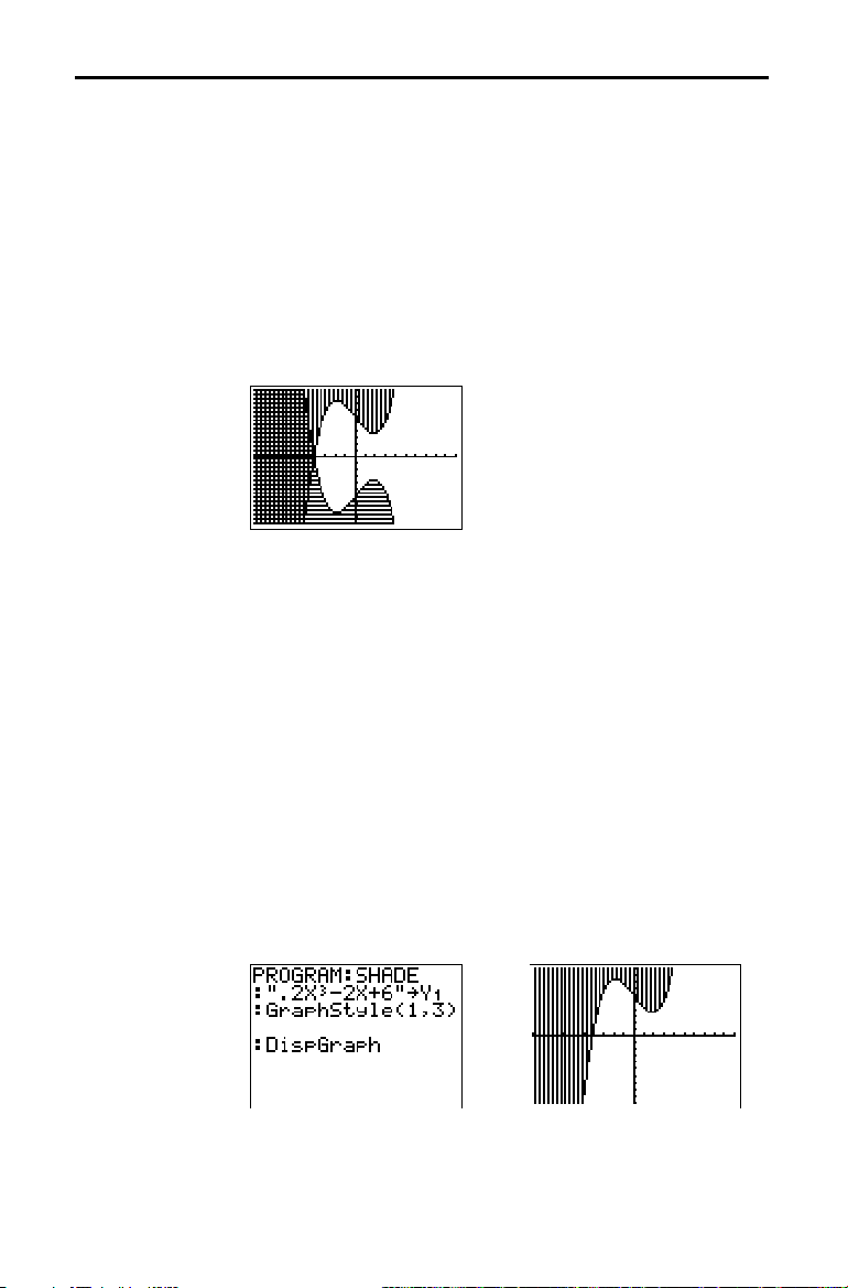
Shading Above and Below
When you select é or ê for two or more functions, the
TI-83 rotates through four shading patterns.
•
Vertical lines shade the first function with a é or
graph style.
•
Horizontal lines shade the second.
•
Negatively sloping diagonal lines shade the third.
•
Positively sloping diagonal lines shade the fourth.
•
The rotation returns to vertical lines for the fifth é or
function, repeating the order described above.
When shaded areas intersect, the patterns overlap.
Note:
When é or ê is selected for a Y= function that graphs a family of
curves, such as
each member of the family of curves.
Y1={1,2,3}X
, the four shading patterns rotate for
ê
ê
Setting a Graph Style from a Program
To set the graph style from a program, select
from the
of the
graphstyle#
the graph style, as shown below.
1
= ç (line)
4
= ê (below)
(animate)
GraphStyle(
For example, when this program is executed in
GraphStyle(1,3)
3-10 Function Graphing
H:GraphStyle(
PRGM CTL
while in the program editor.
function name in the current graphing mode.
Y=
is an integer from
function#,graphstyle#
menu. To display this menu, press
function#
1
to 7 that corresponds to
2
= è (thick)
5
= ë (path)
7
= í (dot)
)
1
Y
sets
to é (above).
is the number
3
6
= é (above)
ì
=
Func
mode,
Page 87

Setting the Viewing Window Variables
The TI-83 Viewing Window
Displaying the Window Variables
The viewing window is the portion of the coordinate plane
defined by
defines the distance between tick marks on the x-axis.
Xmin, Xmax, Ymin, and Ymax. Xscl (X scale)
Yscl
(Y scale) defines the distance between tick marks on the
y-axis. To turn off tick marks, set
Ymax
Xmin
Xscl
Xmax
Yscl
Ymin
Xscl=0 and Yscl=0.
To display the current window variable values, press
p
the default values in
. The window editor above and to the right shows
Func graphing mode and Radian angle
mode. The window variables differ from one graphing
mode to another.
Xres sets pixel resolution (1 through 8) for function graphs
only. The default is
•
Xres=1, functions are evaluated and graphed at each
At
1.
pixel on the x-axis.
•
Xres=8, functions are evaluated and graphed at every
At
eighth pixel along the x-axis.
Tip:
TI-83 to draw graphs more slowly.
Small
Xres
values improve graph resolution but may cause the
Changing a Window Variable Value
To change a window variable value from the window
editor, follow these steps.
1. Press † or } to move the cursor to the window
variable you want to change.
2. Edit the value, which can be an expression.
•
Enter a new value, which clears the original value.
•
Move the cursor to a specific digit, and then edit it.
3. Press
Í, †
, or }. If you entered an expression, the
TI-83 evaluates it. The new value is stored.
Note:
Xmin<Xmax
Ymin<Ymax
and
must be true in order to graph.
Function Graphing 3-11
Page 88

Storing to a Window Variable from the Home Screen or a Program
@
X and @Y
To store a value, which can be an expression, to a window
variable, begin on a blank line and follow these steps.
1. Enter the value you want to store.
2. Press
3. Press
4. Select
¿
.
to display the
1:Window to display the Func window variables
(
secondary menu).
X/Y
•
Press ~ to display the
q
(
secondary menu).
T/
•
Press ~ ~ to display the
(
secondary menu).
U/V/W
menu.
VARS
Par and Pol window variables
Seq window variables
5. Select the window variable to which you want to store a
value. The name of the variable is pasted to the current
cursor location.
6. Press
Í
to complete the instruction.
When the instruction is executed, the TI-83 stores the
value to the window variable and displays the value.
@
@
X
The variables
(1:Window)
X/Y
Y
and
(items 8 and 9 on the
VARS
secondary menu) define the distance from
the center of one pixel to the center of any adjacent pixel
on a graph (graphing accuracy).
from
Xmin, Xmax, Ymin, and Ymax when you display a
X and @Y are calculated
@
graph.
(Xmax N Xmin)
@
X
=
You can store values to
Ymax are calculated from
3-12 Function Graphing
94
@Y =
@
X
@
(Ymax N Ymin)
62
@
Y
and
. If you do, Xmax and
, Xmin,
@
Y
X
, and Ymin.
Page 89

Setting the Graph Format
Displaying the Format Settings
Changing a Format Setting
RectGC, PolarGC
To display the format settings, press y [
FORMAT
]. The
default settings are highlighted below.
RectGC PolarGC
CoordOn CoordOff
GridOff GridOn
AxesOn AxesOff
LabelOff LabelOn
ExprOn ExprOff
Sets cursor coordinates.
Sets coordinates display on or off.
Sets grid off or on.
Sets axes on or off.
Sets axes label off or on.
Sets expression display on or off.
Format settings define a graph’s appearance on the display.
Format settings apply to all graphing modes.
Seq graphing
mode has an additional mode setting (Chapter 6).
To change a format setting, follow these steps.
1. Press †, ~, }, and | as necessary to move the cursor
to the setting you want to select.
2. Press
RectGC (rectangular graphing coordinates) displays the
cursor location as rectangular coordinates
PolarGC (polar graphing coordinates) displays the cursor
location as polar coordinates
The
Í
to select the highlighted setting.
X and Y.
q
R and
.
RectGC/PolarGC setting determines which variables
are updated when you plot the graph, move the freemoving cursor, or trace.
•
RectGC updates X and Y; if CoordOn format is selected,
X and Y are displayed.
•
PolarGC updates X, Y, R, and
q
; if CoordOn format is
selected, R and q are displayed.
Function Graphing 3-13
Page 90

CoordOn, CoordOff
CoordOn (coordinates on) displays the cursor coordinates
at the bottom of the graph. If
ExprOff format is selected,
the function number is displayed in the top-right corner.
CoordOff (coordinates off) does not display the function
number or coordinates.
GridOff, GridOn
AxesOn, AxesOff
LabelOff, LabelOn
ExprOn, ExprOff
Grid points cover the viewing window in rows that
correspond to the tick marks (page 3.11) on each axis.
GridOff does not display grid points.
GridOn displays grid points.
AxesOn displays the axes.
AxesOff does not display the axes.
This overrides the
LabelOff and LabelOn determine whether to display labels
for the axes (
ExprOn and ExprOff determine whether to display the
expression when the trace cursor is active. This format
Y=
LabelOff/LabelOn format setting.
X and Y), if AxesOn format is also selected.
setting also applies to stat plots.
When
ExprOn is selected, the expression is displayed in the
top-left corner of the graph screen.
When
ExprOff and CoordOn both are selected, the number
in the top-right corner specifies which function is being
traced.
3-14 Function Graphing
Page 91

Displaying Graphs
Displaying a New Graph
Pausing or Stopping a Graph
Smart Graph
To display the graph of the selected function or functions,
s
press
.
TRACE, ZOOM
instructions, and
CALC
operations display the graph automatically. As the TI-83
plots the graph, the busy indicator is on. As the graph is
plotted,
X and Y are updated.
While plotting a graph, you can pause or stop graphing.
•
•
Í
Press
to pause; then press
Press É to stop; then press
Í
s
to resume.
to redraw.
Smart Graph is a TI-83 feature that redisplays the last
graph immediately when you press
s
, but only if all
graphing factors that would cause replotting have
remained the same since the graph was last displayed.
If you performed any of these actions since the graph was
last displayed, the TI-83 will replot the graph based on new
values when you press
•
Changed a mode setting that affects graphs
•
Changed a function in the current picture
•
Selected or deselected a function or stat plot
•
Changed the value of a variable in a selected function
•
Changed a window variable or graph format setting
•
Cleared drawings by selecting
•
Changed a stat plot definition
s
.
ClrDraw
Function Graphing 3-15
Page 92

Overlaying Functions on a Graph
On the TI-83, you can graph one or more new functions
without replotting existing functions. For example, store
sin(X) to Y
cos(X) to Y
1
in the Y= editor and press
2
and press
graphed on top of
s
again. The function Y2 is
1
Y
, the original function.
s
. Then store
Graphing a Family of Curves
If you enter a list (Chapter 11) as an element in an
expression, the TI-83 plots the function for each value in
the list, thereby graphing a family of curves. In
Simul
graphing-order mode, it graphs all functions sequentially
for the first element in each list, and then for the second,
and so on.
{2,4,6}sin(X) graphs three functions: 2 sin(X), 4 sin(X), and
6 sin(X).
{2,4,6}sin({1,2,3}X) graphs 2 sin(X), 4 sin(2X), and 6 sin(3X).
Note:
When using more than one list, the lists must have the same
dimensions.
3-16 Function Graphing
Page 93
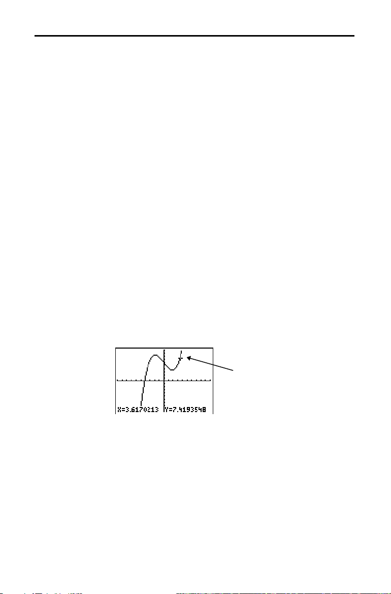
Exploring Graphs with the Free-Moving Cursor
Free-Moving Cursor
Graphing Accuracy
When a graph is displayed, press |, ~, }, or † to move
the cursor around the graph. When you first display the
graph, no cursor is visible. When you press |, ~, }, or †,
the cursor moves from the center of the viewing window.
As you move the cursor around the graph, the coordinate
values of the cursor location are displayed at the bottom of
the screen if
CoordOn format is selected. The Float/Fix
decimal mode setting determines the number of decimal
digits displayed for the coordinate values.
To display the graph with no cursor and no coordinate
values, press
†
, the cursor moves from the same position.
‘
or
Í
. When you press |, ~, }, or
The free-moving cursor moves from pixel to pixel on the
screen. When you move the cursor to a pixel that appears
to be on the function, the cursor may be near, but not
actually on, the function. The coordinate value displayed at
the bottom of the screen actually may not be a point on the
function. To move the cursor along a function, use
r
(page 3.18).
The coordinate values displayed as you move the cursor
approximate actual math coordinates, *accurate to within
the width and height of the pixel. As
Ymax get closer together (as in a ZoomIn) graphing
Xmin, Xmax, Ymin, and
accuracy increases, and the coordinate values more closely
approximate the math coordinates.
Free-moving cursor “on” the curve
Function Graphing 3-17
Page 94
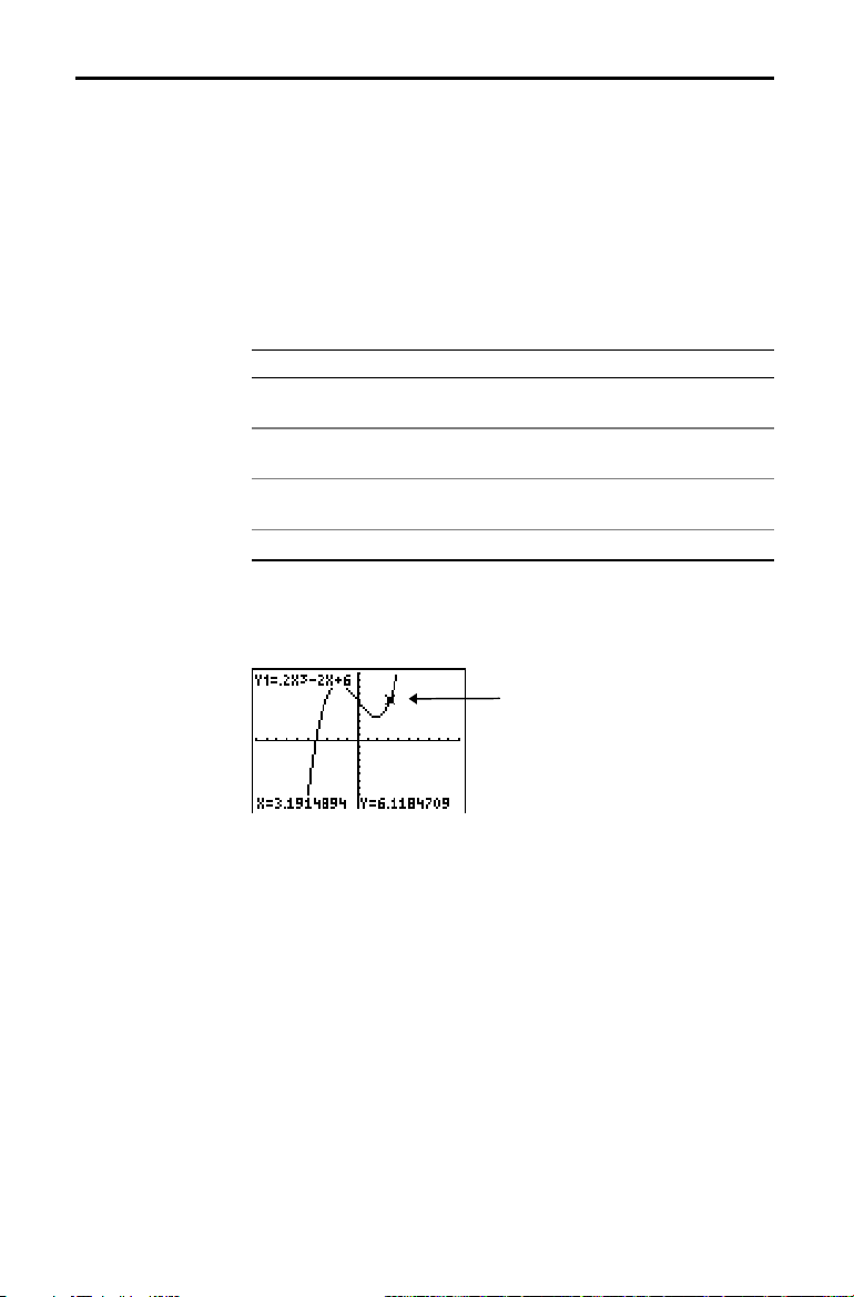
Exploring Graphs with TRACE
Beginning a Trace
Moving the Trace Cursor
Use
the next along a function. To begin a trace, press
the graph is not displayed already, press
to move the cursor from one plotted point to
TRACE
r
r
to display
it. The trace cursor is on the first selected function in the
editor, at the middle X value on the screen. The cursor
Y=
coordinates are displayed at the bottom of the screen if
CoordOn format is selected. The
in the top-left corner of the screen, if
expression is displayed
Y=
ExprOn format is
selected.
To move the TRACE cursor . . . do this:
. . . to the previous or next plotted
press | or ~.
point,
. . . five plotted points on a function
(Xres affects this),
press y | or
~
.
y
. . . to any valid X value on a function, enter a value, and
then press
Í
. . . from one function to another, press } or †.
When the trace cursor moves along a function, the
is calculated from the
function is undefined at an
X value; that is, Y=Yn(X). If the
X value, the Y value is blank.
Trace cursor on the curve
Y value
. If
.
If you move the trace cursor beyond the top or bottom of
the screen, the coordinate values at the bottom of the
screen continue to change appropriately.
Moving the Trace Cursor from Function to Function
To move the trace cursor from function to function, press
†
and }. The cursor follows the order of the selected
functions in the
function at the same
the expression is updated.
3-18 Function Graphing
editor. The trace cursor moves to each
Y=
X value. If ExprOn format is selected,
Page 95
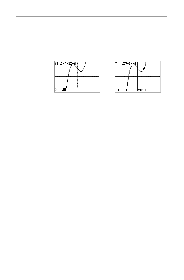
Moving the Trace Cursor to Any Valid X Value
To move the trace cursor to any valid X value on the
current function, enter the value. When you enter the first
digit, an
X= prompt and the number you entered are
displayed in the bottom-left corner of the screen. You can
enter an expression at the
X= prompt. The value must be
valid for the current viewing window. When you have
completed the entry, press
Note:
This feature does not apply to stat plots.
Í
to move the cursor.
Panning to the Left or Right
Quick Zoom
Leaving and Returning to TRACE
Using TRACE in a Program
If you trace a function beyond the left or right side of the
screen, the viewing window automatically pans to the left
or right.
Xmin and Xmax are updated to correspond to the
new viewing window.
While tracing, you can press
Í
to adjust the viewing
window so that the cursor location becomes the center of
the new viewing window, even if the cursor is above or
below the display. This allows panning up and down. After
Quick Zoom, the cursor remains in
When you leave and return to
TRACE
.
TRACE
, the trace cursor is
displayed in the same location it was in when you left
, unless Smart Graph has replotted the graph
TRACE
(page 3.15).
On a blank line in the program editor, press
instruction
Trace is pasted to the cursor location. When the
r
. The
instruction is encountered during program execution, the
graph is displayed with the trace cursor on the first
selected function. As you trace, the cursor coordinate
values are updated. When you finish tracing the functions,
Í
press
to resume program execution.
Function Graphing 3-19
Page 96

Exploring Graphs with the ZOOM Instructions
ZOOM Menu
Zoom Cursor
ZBox
To display the
ZOOM
menu, press
q
. You can adjust the
viewing window of the graph quickly in several ways. All
instructions are accessible from programs.
ZOOM
ZOOM MEMORY
1: ZBox
2: Zoom In
3: Zoom Out
4: ZDecimal
5: ZSquare
6: ZStandard
7: ZTrig
8: ZInteger
9: ZoomStat
0: ZoomFit
When you select
cursor on the graph becomes the zoom cursor (
smaller version of the free-moving cursor (
To define a new viewing window using
Draws a box to define the viewing window.
Magnifies the graph around the cursor.
Views more of a graph around the cursor.
@
Sets
X and @Y to 0.1.
Sets equal-size pixels on the X and Y axes.
Sets the standard window variables.
Sets the built-in trig window variables.
Sets integer values on the X and Y axes.
Sets the values for current stat lists.
Fits YMin and YMax between XMin and XMax.
1:ZBox, 2:Zoom In, or 3:Zoom Out, the
+
), a
+).
ZBox, follow these
steps.
1. Select
1:ZBox from the
menu. The zoom cursor is
ZOOM
displayed at the center of the screen.
2. Move the zoom cursor to any spot you want to define as
a corner of the box, and then press
Í
. When you
move the cursor away from the first defined corner, a
small, square dot indicates the spot.
3. Press |, }, ~, or †. As you move the cursor, the sides
of the box lengthen or shorten proportionately on the
screen.
Note:
To cancel
ZBox
before you press
Í
4. When you have defined the box, press
, press
Í
‘
.
to replot
the graph.
To use ZBox to define another box within the new graph,
repeat steps 2 through 4. To cancel
3-20 Function Graphing
ZBox, press
‘
.
Page 97

Zoom In, Zoom Out
Zoom In magnifies the part of the graph that surrounds the
cursor location.
graph, centered on the cursor location. The
YFact settings determine the extent of the zoom.
Zoom Out displays a greater portion of the
XFact and
To zoom in on a graph, follow these steps.
1. Check
2. Select
XFact and YFact (page 3
2:Zoom In from the
.
24); change as needed.
menu. The zoom
ZOOM
cursor is displayed.
3. Move the zoom cursor to the point that is to be the
center of the new viewing window.
4. Press
Í
. The TI-83 adjusts the viewing window by
XFact and YFact; updates the window variables; and
replots the selected functions, centered on the cursor
location.
5. Zoom in on the graph again in either of two ways.
•
To zoom in at the same point, press
•
To zoom in at a new point, move the cursor to the
Í
.
point that you want as the center of the new viewing
window, and then press
To zoom out on a graph, select
Í
.
3:Zoom Out and repeat
steps 3 through 5.
To cancel
Zoom In or Zoom Out, press
‘
.
ZDecimal
ZSquare
ZDecimal replots the functions immediately. It updates the
window variables to preset values, as shown below. These
values set
@
X and @Y equal to 0.1 and set the X and Y value
of each pixel to one decimal place.
Xmin=L4.7 Ymin=L3.1
Xmax=4.7 Ymax=3.1
Xscl=1 Yscl=1
ZSquare
replots the functions immediately. It redefines the
viewing window based on the current values of the
window variables. It adjusts in only one direction so that
@X=@
Y
, which makes the graph of a circle look like a circle.
Xscl and Yscl remain unchanged. The midpoint of the
current graph (not the intersection of the axes) becomes
the midpoint of the new graph.
Function Graphing 3-21
Page 98

ZStandard
ZTrig
ZStandard replots the functions immediately. It updates the
window variables to the standard values shown below.
Xmin=L10 Ymin=L10 Xres=1
Xmax=10 Ymax=10
Xscl=1 Yscl=1
ZTrig
replots the functions immediately. It updates the
window variables to preset values that are appropriate for
plotting trig functions. Those preset values in
Radian mode
are shown below.
Xmin=L(47à24)
Xmax=(47à24)
Xscl=p/2 Yscl=1
p
p
Ymin=L4
Ymax=4
ZInteger
ZoomStat
ZoomFit
ZInteger
shown below. To use
redefines the viewing window to the dimensions
ZInteger, move the cursor to the point
that you want to be the center of the new window, and
then press
@
X=1 Xscl=10
@
Y=1 Yscl=10
ZoomStat
Í
;
ZInteger replots the functions.
redefines the viewing window so that all
statistical data points are displayed. For regular and
modified box plots, only
ZoomFit replots the functions immediately. ZoomFit
Xmin and Xmax are adjusted.
recalculates YMin and YMax to include the minimum and
maximum
current
Y values of the selected functions between the
XMin and XMax. XMin and XMax are not changed.
3-22 Function Graphing
Page 99

Using ZOOM MEMORY
ZOOM MEMORY Menu
ZPrevious
ZoomSto
ZoomRcl
To display the
ZOOM MEMORY
1:ZPrevious
2:ZoomSto
3:ZoomRcl
4:SetFactors
ZPrevious
replots the graph using the window variables of
ZOOM MEMORY
menu, press
Uses the previous viewing window.
Stores the user-defined window.
Recalls the user-defined window.
...
Changes
Zoom In
and
q ~
Zoom Out
.
factors.
the graph that was displayed before you executed the last
instruction.
ZOOM
ZoomSto
immediately stores the current viewing window.
The graph is displayed, and the values of the current
window variables are stored in the user-defined
variables
ZXres
ZXmin, ZXmax, ZXscl, ZYmin, ZYmax, ZYscl
.
ZOOM
, and
These variables apply to all graphing modes. For example,
changing the value of
Par
in
mode.
ZoomRcl
graphs the selected functions in a user-defined
ZXmin
in
Func
mode also changes it
viewing window. The user-defined viewing window is
determined by the values stored with the
ZoomSto
instruction. The window variables are updated with the
user-defined values, and the graph is plotted.
Function Graphing 3-23
Page 100
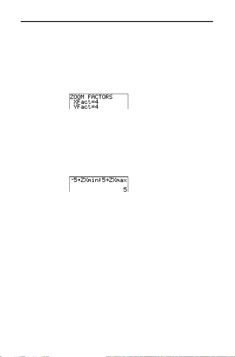
ZOOM FACTORS
The zoom factors, XFact and YFact, are positive numbers
(not necessarily integers) greater than or equal to 1. They
define the magnification or reduction factor used to
In
or Zoom Out around a point.
Zoom
Checking XFact and YFact
Changing XFact and YFact
Using ZOOM MEMORY Menu Items from the Home Screen or a Program
To display the
ZOOM FACTORS
review the current values for
4:SetFactors from the
ZOOM MEMORY
screen, where you can
XFact and YFact, select
menu. The values
shown are the defaults.
You can change XFact and YFact in either of two ways.
•
Enter a new value. The original value is cleared
automatically when you enter the first digit.
•
Place the cursor on the digit you want to change, and
then enter a value or press { to delete it.
From the home screen or a program, you can store directly
to any of the user-defined
ZOOM
variables.
From a program, you can select the ZoomSto and ZoomRcl
instructions from the
ZOOM MEMORY
menu.
3-24 Function Graphing
 Loading...