

Page 1

®
ME•Pro
Mechanical Engineeri ng
User’s Manual
A software Application
for the TI-89 and TI-92 Plus
Version 1.0 by
da V
inci Technologies Group Inc
Page 2

ME••••Pro®
A software Application
For TI-89 and TI-92 Plus
User’s Guide
August 2000
© da Vinci Technologies Group, Inc.
Rev. 1.0
da Vinci Technologies Group, Inc.
1600 S.W. Western Blvd
Suite 250
Corvallis, OR 97333
www.dvtg.com
2
Page 3

Notice
This manual and the examples contained herein are provided “as is” as a supplement to ME•
Pro
application software available from Texas Instruments for TI-89, and TI-92 Plus platforms. da Vinci
Te chnologies Gro up, Inc. (“da V inci”) makes no warranty of any kind with r egard t o this manual
or the accompanying software, including, but not limited to, the implied warranties of
merchantability and fitness for a particular purpose. da Vinci shall not be lia ble for any errors or f or
incidenta l or consequ ent ial dama ges in connec tion with the furnishing, per f ormance, or use of this
manual , or the examp l es her ei n .
Copyr ight da Vinci Technologies Gr oup, Inc. 2000. All rights reserved.
PocketProfessional and ME•Pro are registered trademarks of da Vinci Technologies Group, Inc.
TI-GRAPH LINK is a trademark of Texas Instruments Incorporated, and Acrobat is a registered
trademark of Adobe Systems Incorporated.
We welcome your comments on the software and the manual. Forward your comments, preferably by
e-mail, to da Vinci at support@dvtg.com.
Acknowledgements
The ME•Pro software was developed by Chris Bunsen, Dave Conklin, Michael Conway, Curtis Gammel, and
Megh a Shyam with the gene r ou s support of TI’ s developmen t te a m . The user ’ s gu ide wa s developed by Mi cha e l
Conway, Curtis Gammel, Melinda Shaffer, and Megha Shyam. Many helpful comments from the testers at
Texas Instrume nts and other locations during β testing phase is gratefully acknowledged.
3
Page 4

Table of Contents
TABLE OF CONTENTS4
HAPTER
C
NTRODUCTION TO
1: I
1.1 Key Featur es of ME•Pro....................................................................................................12
1.2 Purchasing, Downloading and Installing ME•Pro...............................................................13
1.3 Ordering a Manual.............................................................................................................13
1.4 Memory Requirements......................................................................................................13
1.5 Differences between TI-89 and TI-92 plus.......................................................................... 13
1.6 Starting ME•Pro................................................................................................................13
1.7 How to use this Manual......................................................................................................14
1.8 Manual Disclaimer............................................................................................................. 14
1.9 Summary.................................................................................................................... ....... 15
PART I: ANALYSIS……………………………………………………………………………………...16
HAPTER
C
NTRODUCTION TO ANALYSIS
2: I
2.1 Introduction.......................................................................................................................17
2.2 Features of Analysis...........................................................................................................18
2.3 Finding Analysis................................................................................................................18
2.4 Solving a Problem in Analysis ...........................................................................................18
2.5 Tips for Analysis ...............................................................................................................20
2.6 Function keys ....................................................................................................................20
2.7 Session Folders, Variable Names.......................................................................................22
2.8 Overwriting of variable values in graphing......................................................................... 22
2.9 Reserved Variables............................................................................................................22
HAPTER
C
TEAM TABLES
3: S
3.1 Saturated Steam Properties................................................................................................. 23
3.2 Superheated Steam Properties............................................................................................23
3.3 Air Properties ....................................................................................................................23
3.4 Using Steam Tables ...........................................................................................................24
3.5 Validity Range for Temperature and Pressure..................................................................... 25
HAPTER
C
HERMOCOUPLES
4: T
4.1 Introduction.......................................................................................................................26
4.2 Using the Thermocouples Function ....................................................................................26
4.3 Basis for Temperature/Voltage Conversions.......................................................................27
HAPTER
C
APITAL BUDGETING
5: C
5.1 Using Capital Budgeting.................................................................................................... 28
HAPTER
C
FOR MECHANICAL ENGINEERS
6: EE
6.1 Impedance Calculations..................................................................................................... 32
6.2 Circuit Performance...........................................................................................................33
6.3 Wye ↔ ∆ Conversion........................................................................................................ 34
HAPTER
C
7: E
FFLUX
..........................................................................................................................36
7.1 Constant Liquid Level........................................................................................................36
7.2 Varying Liquid Level......................................................................................................... 36
7.3 Conical Vessel................................................................................................................... 37
7.4 Horizontal Cylinder ........................................................................................................... 38
7.5 Large Rectangular Orifice.................................................................................................. 38
7.6 ASME Weirs......................................................................................................................... 39
7.6.1 Rectangular Notch .......................................................................................................... 39
7.6.2 Triangular Weir ..............................................................................................................39
7.6.3 Suppressed Weir .............................................................................................................40
7.6.4 Cipolletti Weir................................................................................................................40
HAPTER
C
ECTION PROPERTIES
8: S
8.1 Rectangle........................................................................................................................... 42
••••
RO
P
ME
............................................................................................12
..........................................................................................17
................................................................................................................23
............................................................................................................26
.......................................................................................................28
...................................................................................32
.....................................................................................................42
ME⋅Pro for TI-89, TI-92 Plus
Table of Contents
4
Page 5

8.2 Hollow Rectangle.............................................................................................................. 43
8.3 Circle.................................................................................................................................43
8.4 Circular Ring.....................................................................................................................44
8.5 Hollow Circle....................................................................................................................45
8.6 1 Section - Uneven.............................................................................................................45
8.7 I Section - Even ................................................................................................................. 46
8.8 C Section........................................................................................................................... 47
8.9 T Section ...........................................................................................................................48
8.10 Trapezoid.........................................................................................................................48
8.11 Polygon ........................................................................................................................... 49
8.12 Hollow Polygon............................................................................................................... 50
HAPTER
C
ARDNESS NUMBER
9: H
.......................................................................................................52
9.1 Compute Hardness Number ...............................................................................................52
PART II: EQUATIONS………………………………………………………………………………… ...54
HAPTER
C
NTRODUCTION TO EQUATIONS
10: I
.....................................................................................55
10.1 Solving a Set of Equations ...............................................................................................55
10.2 Viewing an Equation or Result in Pretty Print ..................................................................56
10.3 Viewing a Result in different units ...................................................................................56
10.4 Viewing Multiple Solutions..............................................................................................57
10.5 when (…) - conditional constraints when solving equations .............................................. 58
10.5 Arbitrary Integers for periodic solutions to trigonometric functions................................... 58
10.7 Partial Solutions...............................................................................................................59
10.8 Copy/Paste.......................................................................................................................59
10.9 Graphing a Function.........................................................................................................59
10.10 St oring a nd re c alling variabl e value s in M E•Pro-creation of session folders.................... 61
10.11 solve, nsolve, and csolve and user-defined functions (UDF)........................................ 61
10.12 Entering a guessed value for the unknown using nsolve ..................................................61
10.13 Why can't I compute a solution?.....................................................................................62
10.14 Care in choosing a consistent set of equations.................................................................62
10.15 Not e s for the adva nced user in troubleshooting calculations ............................................ 62
HAPTER
C
EAMS AND COLUMNS
11: B
..................................................................................................64
11.1 Simple Beams......................................................................................................................64
11.1.1 Uniform Load...............................................................................................................64
11.1.2 Point Load ....................................................................................................................66
11.1.3 Moment Load ............................................................................................................... 68
11.2 Cantilever Beams.................................................................................................................70
11.2.1 Uniform Load...............................................................................................................70
11.2.2 Point Load ....................................................................................................................71
11.2.3 Moment Load ............................................................................................................... 73
11.3. Columns............................................................................................................................. 75
11.3.1 Buckling.......................................................................................................................75
11.3.2 Eccentricity, Axial Load................................................................................................ 76
11.3.3 Secant Formula ............................................................................................................. 77
11.3.4 Imperfections in Columns .............................................................................................79
11.3.5 Inelastic Buckling .........................................................................................................81
HAPTER
C
12: EE
FOR MES
................................................................................................................83
12.1 Basic Electricity...................................................................................................................83
12.1.1 Resistance Formulas......................................................................................................83
12.1.2 Ohm’s Law and Power..................................................................................................84
12.1.3 Temperature Effect ....................................................................................................... 85
12.2 DC Motors...........................................................................................................................86
12.2.1 DC Series Motor ...........................................................................................................86
12.2.2 DC Shunt Motor............................................................................................................88
12.3 DC Generators..................................................................................................................... 90
12.3.1 DC Series Generator ..................................................................................................... 90
12.3.2 DC Shunt Generator......................................................................................................91
ME⋅Pro for TI-89, TI-92 Plus
Table of Contents
5
Page 6

12.4 AC Motors...........................................................................................................................92
12.4.1 Three φ Induction Motor I............................................................................................. 92
12.4.2 Three φ Induction Motor II............................................................................................ 94
12.4.3 1 Induction Motor......................................................................................................... 96
HAPTER
C
13: G
AS LAWS
.....................................................................................................................98
13.1 Ideal Gas Laws....................................................................................................................98
13.1.1 Ideal Gas Law...............................................................................................................98
13.1.2 Constant Pressure.......................................................................................................... 99
13.1.3 Constant Volume........................................................................................................ 101
13.1.4 Constant Temperature.................................................................................................103
13.1.5 Internal Energy/Enthalpy............................................................................................. 104
13.2 Kinetic Gas Theory........................................................................................................ 106
13.3 Real Gas Laws................................................................................................................... 108
13.3.1 van der Waals: Specific Volume..................................................................................108
13.3.2 van der Waals: Molar form.......................................................................................... 109
13.3.3 Redlich-Kwong: Sp.Vol.............................................................................................. 110
13.3.4 Redlich-Kwong: Molar................................................................................................112
13.4 Reverse Adiabatic.......................................................................................................... 113
13.5 Polytropic Process.......................................................................................................... 115
HAPTER
C
14: H
EAT TRANSFER
.........................................................................................................118
14.1 Basic Transfer Mechanisms ............................................................................................... 118
14.1.1 Conduction ................................................................................................................. 118
14.1.2 Convection..................................................................................................................120
14.1.3 Radiation .................................................................................................................... 121
14.2 1 1D Heat Transfer ................................................................................................................ 122
14.2.1 Conduction..................................................................................................................... 122
14.2.1.1 Plane Wall ............................................................................................................... 122
14.2.1.2 Convective Source ................................................................................................... 123
14.2.1.3 Radiative Source......................................................................................................125
14.2.1.4 Plate and Two Fluids................................................................................................127
14.2.2 Electrical Analogy .......................................................................................................... 128
14.2.2.1 Two Conductors in Series......................................................................................... 129
14.2.2.2 Two Conductors in Parallel ...................................................................................... 131
14.2.2.3 Parallel-Series.......................................................................................................... 132
14.2.3 Radial Systems ...............................................................................................................135
14.2.3.1 Hollow Cylinder....................................................................................................... 135
14.2.3.2 Hollow Sphere ......................................................................................................... 136
14.2.3.3 Cylinder with Insulation Wrap.................................................................................. 137
14.2.3.4 Cylinder - Critical radius..........................................................................................139
14.2.3.5 Sphere - Critical radius.............................................................................................141
14.3 Semi-Infinite Solid.............................................................................................................142
14.3.1 Step Change Surface Temperature............................................................................... 142
14.3.2 Constant Surface Heat Flux......................................................................................... 143
14.3.3 Surface Convection..................................................................................................... 145
14.4 Radiation........................................................................................................................... 146
14.4.1 Blackbody Radiation................................................................................................... 146
14.4.2 Non-Blackbody radiation ............................................................................................148
14.4.3 Thermal Radiation Shield............................................................................................ 149
HAPTER
C
HERMODYNAMICS
15: T
.....................................................................................................152
15.1 Fundamentals................................................................................................................. 152
15.2 System Properties .............................................................................................................. 153
15.2.1 Energy Equations........................................................................................................ 153
15.2.2 Maxwell Relations ...................................................................................................... 155
15.3 Vapor and Gas Mixture...................................................................................................... 157
15.3.1 Saturated Liquid/Vapor ............................................................................................... 157
15.3.2 Compressed Liquid-Sub cooled ...................................................................................159
ME⋅Pro for TI-89, TI-92 Plus
Table of Contents
6
Page 7

15.4 Ideal Gas Properties........................................................................................................... 160
15.4.1 Specific Heat...............................................................................................................160
15.4.2 Quasi-Equilibrium Compression..................................................................................162
15.5 First Law...............................................................................................................................163
15.5.1 Total System Energy...................................................................................................163
15.5.2 Closed System: Ideal Gas...............................................................................................167
15.5.2.1 Constant Pressure.....................................................................................................167
15.5.2.2 Binary Mixture......................................................................................................... 169
15.6 Second Law........................................................................................................................... 171
15.6.1 Heat Engine Cycle .......................................................................................................... 171
15.6.1.1 Carnot Engine..........................................................................................................171
15.6.1.2 Diesel Cycle............................................................................................................. 173
15.6.1.3 Dual Cycle............................................................................................................... 177
15.6.1.4 Otto Cycle................................................................................................................180
15.6.1.5 Brayton Cycle .......................................................................................................... 184
15.6.2 Clapeyron Equation.....................................................................................................186
HAPTER
C
ACHINE DESIGN
16: M
.......................................................................................................188
16.1 Stress: Machine Elements .................................................................................................. 188
16.1.1 Cylinders .................................................................................................................... 188
16.1.2 Rotating Rings............................................................................................................ 189
16.1.3 Pressure and Shrink Fits.............................................................................................. 190
16.1.4 Crane Hook................................................................................................................. 192
16.2 Hertzian Stresses................................................................................................................193
16.2.1 Two Spheres...............................................................................................................193
16.2.2 Two Cylinders............................................................................................................ 195
16.3.1 Bearing Life................................................................................................................ 197
16.3.2 Petroff's law................................................................................................................ 198
16.3.3 Pressure Fed Bearings................................................................................................. 199
16.3.4 Lewis Formula............................................................................................................200
16.3.5 AGMA Stresses.......................................................................................................... 201
16.3.6 Shafts..........................................................................................................................203
16.3.7 Clutches and Brakes ........................................................................................................... 204
16.3.7.1 Clutches....................................................................................................................... 204
16.3.7.1.1 Clutches ................................................................................................................ 204
16.3.7.2 Uniform Wear - Cone Brake.....................................................................................206
16.3.7.3 Uniform Pressure - Cone Brake................................................................................ 207
16.4 Spring Design........................................................................................................................208
16.4.1 Bending.......................................................................................................................... 208
16.4.1.1 Rectangular Plate.....................................................................................................208
16.4.1.2 Triangular Plate........................................................................................................ 209
16.4.1.3 Semi-Elliptical......................................................................................................... 210
16.4.2 Coiled Springs................................................................................................................ 212
16.4.2.1 Cylindrical Helical - Circular wire............................................................................ 212
16.4.2.2 Rectangular Spiral.................................................................................................... 213
16.4.3 Torsional Spring............................................................................................................. 215
16.4.3.1 Circular Straight Bar ................................................................................................215
16.4.3.2 Rectangular Straight Bar...........................................................................................216
16.4.4 Axial Loaded.................................................................................................................. 217
16.4.4.1 Conical Circular Section........................................................................................... 217
16.4.4.2 Cylindrical - Helical..................................................................................................... 219
16.4.4.2.1 Rectangular Cross Section .....................................................................................219
16.4.4.2.2 Circular Cross Section ........................................................................................... 220
HAPTER
C
UMPS AND HYDRAULICS
17: P
............................................................................................222
17.1 Basic Definitions ...........................................................................................................222
17.2 Pump Power .................................................................................................................. 223
17.3 Centrifugal Pumps.............................................................................................................225
ME⋅Pro for TI-89, TI-92 Plus
Table of Contents
7
Page 8

17.3.1 Affinity Law-Variable Speed.......................................................................................225
17.3.2 Affinity Law-Constant Speed......................................................................................226
17.3.3 Pump Similarity.......................................................................................................... 227
17.3.4 Centrifugal Compressor............................................................................................... 228
17.3.5 Specific Speed ............................................................................................................229
HAPTER
C
AVES AND OSCILLATION
18: W
...........................................................................................231
18.1 Simple Harmonic Motion...................................................................................................231
18.1.1 Linear Harmonic Oscillation........................................................................................231
18.1.2 Angular Harmonic Oscillation..................................................................................... 232
18.2 Pendulums.........................................................................................................................233
18.2.1 Simple Pendulum........................................................................................................233
18.2.2 Physical Pendulum...................................................................................................... 235
18.2.3 Torsional Pendulum....................................................................................................236
18.3 Natural and Forced Vibrations.............................................................................................. 236
18.3.1 Natural Vibrations...........................................................................................................236
18.3.1.1 Free Vibration..........................................................................................................236
18.3.1.2 Overdamped Case (ξ>1)........................................................................................... 238
18.3.1.3 Critical Damping (ξ=1) ............................................................................................ 239
18.3.1.4 Underdamped Case (ξ<1)......................................................................................... 241
18.3.2 Forced Vibrations ........................................................................................................... 244
18.3.2.1 Undamped Forced Vibration.....................................................................................244
18.3.2.2 Damped Forced Vibration ........................................................................................ 245
18.3.3 Natural Frequencies...........................................................................................................247
18.3.3.1 Stretched String........................................................................................................ 247
18.3.3.2 Vibration Isolation ................................................................................................... 248
18.3.3.3 Uniform Beams............................................................................................................249
18.3.3.3.1 Simply Supported..................................................................................................250
18.3.3.3.2 Both Ends Fixed.................................................................................................... 251
18.3.3.3.3 1 Fixed End / 1 Free End....................................................................................... 252
18.3.3.3.4 Both Ends Free...................................................................................................... 254
18.3.3.4 Flat Plates.................................................................................................................... 255
18.3.3.4.1 Circular Flat Plate.................................................................................................. 255
18.3.3.4.2 Rectangular Flat Plate............................................................................................257
HAPTER
C
EFRIGERATION AND AIR CONDITIONING
19: R
...................................................................259
19.1 Heating Load.................................................................................................................259
19.2 Refrigeration......................................................................................................................261
19.2.1 General Cycle .............................................................................................................261
19.2.2 Reverse Carnot............................................................................................................ 262
19.2.3 Reverse Brayton.......................................................................................................... 263
19.2.4 Compression Cycle.....................................................................................................264
HAPTER
C
TRENGTH MATERIALS
20: S
...............................................................................................267
20.1 Stress and Strain Basics ..................................................................................................... 267
20.1.1 Normal Stress and Strain.............................................................................................267
20.1.2 Volume Dilation.........................................................................................................268
20.1.3 Shear Stress and Modulus............................................................................................ 269
20.2 Load Problems...................................................................................................................270
20.2.1 Axial Load.................................................................................................................. 270
20.2.2 Temperature Effects....................................................................................................271
20.2.3 Dynamic Load ............................................................................................................272
20.3 Stress Analysis ..................................................................................................................274
20.3.1 Stress on an Inclined Section ....................................................................................... 274
20.3.2 Pure Shear...................................................................................................................275
20.3.3 Principal Stresses........................................................................................................276
20.3.4 Maximum Shear Stress................................................................................................277
20.3.5 Plane Stress - Hooke's Law..........................................................................................278
20.4 Mohr’s Circle Stress..........................................................................................................280
ME⋅Pro for TI-89, TI-92 Plus
Table of Contents
8
Page 9

20.4 Mohr’s Circle Stress.......................................................................................................280
20.5 Torsion.............................................................................................................................. 281
20.5.1 Pure Torsion............................................................................................................... 281
20.5.2 Pure Shear...................................................................................................................283
20.5.3 Circular Shafts............................................................................................................ 284
20.5.4 Torsional Member.......................................................................................................285
HAPTER
C
LUID MECHANICS
21: F
.....................................................................................................288
21.1 Fluid Properties .......................................................................................................... ....... 288
21.1.1 Elasticity..................................................................................................................... 288
21.1.2 Capillary Rise............................................................................................................. 289
21.2 Fluid Statics............................................................................................................. ............. 291
21.2 1 Pressure Variation........................................................................................................... 291
21.2.1.1 Uniform Fluid.......................................................................................................... 291
21.2.1.2 Compressible Fluid..................................................................................................292
21.2.1 Pressure Variation........................................................................................................... 292
21.2.1.3 Troposphere.............................................................................................................292
21.2.1.4 Stratosphere............................................................................................................. 293
21.2.2.1 Floating Bodies........................................................................................................294
21.2.2.2 Inclined Plane/Surface.............................................................................................. 296
21.3 Fluid Dynamics.................................................................................................................297
21.3.1 Bernoulli Equation...................................................................................................... 297
21.3.2 Reynolds Number ....................................................................................................... 299
21.3.3 Equivalent Diameter....................................................................................................300
21.3.4 Fluid Mass Acceleration.................................................................................................. 302
21.3.4.1 Linear Acceleration .................................................................................................. 302
21.3.4.2 Rotational Acceleration ............................................................................................303
21.4 Surface Resistance............................................................................................................. 304
21.4.1 Laminar Flow – Flat Plate ........................................................................................... 304
21.4.2 Turbulent Flow – Flat Plate.........................................................................................306
21.4.3 Laminar Flow on an Inclined Plane..............................................................................309
21.5 Flow in Conduits ................................................................................................................... 311
21.5.1 Lamina r F l ow: Smooth Pipe....................................................................................... 311
21.5.2 Turbulent Flow: Smooth Pi pe..................................................................................... 313
21.5.3 Turbulent Flow: Rough Pipe....................................................................................... 316
21.5.4 Flow pipe Inlet............................................................................................................ 319
21.5.5 Series Pipe System...................................................................................................... 321
21.5.6 Parallel Pipe System .................................................................................................... 322
21.5.7 Venturi Meter.................................................................................................................324
21.5.7.1 Incompressible Flow ................................................................................................ 324
21.5.7.2 Compressible Flow...................................................................................................327
21.6 Impulse/Momentum............................................................................................................... 330
21.6.1 Jet Propulsion ............................................................................................................. 330
21.6.2 Open Jet..........................................................................................................................331
21.6.2.1 Vertical Plate ........................................................................................................... 331
21.6.2.2 Horizontal Plate ....................................................................................................... 332
21.6.2.3 Stationary Blade.......................................................................................................333
21.6.2.4 Moving Blade..........................................................................................................335
HAPTER
C
YNAMICS AND STATICS
22: D
.............................................................................................338
22.1 Laws of Motion ............................................................................................................. 338
22.2 Constant A ccelerat ion........................................................................................................ 340
22.2.1 Linear Motion............................................................................................................. 340
22.2.2 Free Fall .....................................................................................................................341
22.2.3 Circular Motion........................................................................................................... 342
22.3 Angular Motion................................................................................................................. 343
22.3.1 Rolling/Rotation.......................................................................................................... 343
22.3.2 Forces in Angular Motion............................................................................................ 345
ME⋅Pro for TI-89, TI-92 Plus
Table of Contents
9
Page 10

22.3.3 Gyroscope Motion.......................................................................................................346
22.4 Projectile Motion ........................................................................................................... 347
22.5 Collisions..............................................................................................................................349
22.5.1 Elastic Collisions ............................................................................................................ 349
22.5.1.1 1D Collision............................................................................................................. 349
22.5.1.2 2D Collisions........................................................................................................... 350
22.5.2 Inelastic Collisions.......................................................................................................... 351
22.5.2.1 1D Collisions........................................................................................................... 351
22.5.2.2 Oblique Collisions.................................................................................................... 352
22.6 Gravitational Effects.......................................................................................................... 354
22.6.1 Law of Gravitation...................................................................................................... 354
22.6.2 Kepler's Laws ............................................................................................................. 356
22.6.3 Satellite Orbit..............................................................................................................358
22.7 Friction..............................................................................................................................360
22.7.1 Frictional Force........................................................................................................... 360
22.7.2 Wedge........................................................................................................................ 362
22.7.3 Rotating Cylinder........................................................................................................363
22.8 Statics................................................................................................................................364
22.8.1 Parabolic cable............................................................................................................ 364
22.8.2 Catenary cable............................................................................................................365
PART III: REFERENCE ……………………………………………………………………….368
HAPTER
C
NTRODUCTION TO REFERENCE
23: I
...................................................................................369
23.1 Introduction................................................................................................................... 369
23.2 Finding Reference.......................................................................................................... 369
23.3 Reference Screens.......................................................................................................... 370
23.4 Using Reference Tables .................................................................................................370
HAPTER
C
NGINEERING CONSTANTS
24: E
..........................................................................................372
24.1 Using Constants............................................................................................................. 372
HAPTER
C
25: T
RANSFORMS
..............................................................................................................374
25.1 Using Transforms ..........................................................................................................374
HAPTER
C
ALVES AND FITTING LOSS
26: V
.........................................................................................376
26.1 Valves and Fitting Loss Screens.....................................................................................376
HAPTER
C
RICTION COEFFICIENTS
27: F
............................................................................................377
27.1 Friction Coefficients Screens..........................................................................................377
HAPTER
C
ELATIVE ROUGHNESS OF PIPES
28: R
................................................................................378
28.1 Relative Roughness Screens ........................................................................................... 378
HAPTER
C
ATER-PHYSICAL PROPERTIES
29: W
...................................................................................379
29.1 Water-Physical Properties Screens..................................................................................379
HAPTER
C
ASES AND VAPORS
30: G
.....................................................................................................380
30.1 Gases and Vapors S creens.............................................................................................. 381
HAPTER
C
HERMAL PROPERTIES
31: T
................................................................................................382
31.1 Thermal Properties Screens............................................................................................ 382
HAPTER
C
UELS AND COMBUSTION
32: F
............................................................................................383
32.1 Fuels and Combustion Screens.......................................................................................383
HAPTER
C
33: R
EFRIGERANTS
...........................................................................................................385
33.1 Refrigerants Screens ...................................................................................................... 386
HAPTER
C
34: SI P
REFIXES
...............................................................................................................387
34.1 Using SI Prefixes........................................................................................................... 387
HAPTER
C
REEK ALPHABET
35: G
......................................................................................................388
PART IV: APPENDIX AND INDEX…………………………………………………………….…….389
PPENDIX
A
REQUENTLY ASKED QUESTIONS
A F
.................................................................................390
A.1 Questions and Answers...................................................................................................390
A.2 General Questions........................................................................................................... 390
A.3 Analysis Questions.......................................................................................................... 392
A.4 Equations Questions........................................................................................................ 392
A.5 Graphing.........................................................................................................................395
ME⋅Pro for TI-89, TI-92 Plus
Table of Contents
10
Page 11

A.6 Reference........................................................................................................................ 396
PPENDIX
A
B W
ARRANTY
ECHNICAL SUPPORT
, T
................................................................................397
B.1 da Vinci License Agreement............................................................................................397
B.2 How to Contact Customer Support................................................................................... 398
PPENDIX
A
C: TI-89 & TI-92 P
LUS
EYSTROKE AND DISPLAY DIFFERENCES
- K
...................................399
C.1 Display Property Differences between the TI-89 and TI-92 Plus......................................399
C.2 Keyboard Differences Between TI-89 and TI-92 Plus ..................................................... 400
PPENDIX
A
RROR MESSAGES
D E
.......................................................................................................404
D.1 General Error Messages..................................................................................................404
D.2 Analysis Error Messages................................................................................................. 405
D.3 Equation Messages.......................................................................................................... 405
D.4 Reference Error Messages...............................................................................................406
PPENDIX E: SYSTEM VARIABLES AND RESERVED NAMES
A
.............................................................407
INDEX ……………………………………………………………………………………………………408
ME⋅Pro for TI-89, TI-92 Plus
Table of Contents
11
Page 12

Chapter 1: Introduction to ME••••Pro
Thank you for purchasing the ME•Pro, a m ember of the PocketProfessiona l® Pro software series designed
by da Vin ci Technologies Group, Inc., t o meet the porta ble computing needs of student s an d p rofessionals
in mechanical engineering. The software is organized in a hierarchical manner so t hat the topics easy to
find. We hope that you will find the ME•Pro to be a valuable companion in your career as a student and a
professional of m echanical engi neering.
Topics in this chapter include:
Key Features of ME•Pro
Purchasing, Download and Installing ME•Pro
Ordering a Manual
Memory Requirements
Differences between the TI-89 and TI-92 Plus
Starting the ME•Pro
How to use this Manual
Manual Disclaimer
Summary
1.1 Key Features of ME••••Pro
The manual is organized into t hree sections representing the main menu headings of ME•Pro.
Analysis Equations Reference
Steam Tables Beams and Columns Engineering Constants
Thermocouples EE For MEs Transforms
Capital Budgeting Gas Laws Valves/Fitting Loss
EE For MEs Heat Transfer Friction Coefficients
Efflux Thermodynamics Roughness of Pipes
Section Properties Machine Design Water Physical Properties
Hardness Number Pumps and Hydraulic Machines Gases and Vapors
Waves and Oscillation Thermal Properties
Refrigeration and Air Conditioning Fuels and Combustion
Strength Materials Refrigerants
Fluid Mechanics SI Prefixes
Dynamics and Statics Greek Alphabet
Thes e main topi c headings a re further divi d ed int o sub- topics. A brief descri ption of the main sections of
the software is listed below:
Analysis: Chapt er s 2-9
Analysis is organized into 7 topics and 25 sub-topics. The software tools available in this section
incorporate a va riety of an alysis methods used by mech anical en g ineers. Examples include Steam
Tables, Thermocouple Calculations, EE for MEs; Efflux, Section Properties, Hardness Number
Computations and Capital Budgeting. Wh er e appropriate, dat a en t er ed supports commonly used units.
Equations: Chapters 10-22
This section contains over 1000 equations organized under 12 major subjects in over 150 sub -topics. The
equations in each sub-topic have been selected to provide maximum coverage of the subject material. In
ME⋅Pro for TI-89, TI-92 Plus
Chapter 1 - Introduction to ME-Pro
12
Page 13

addition, the math engine is able to compute multiple or partial solutions to the equation sets. The
computed values are filtered to identify results that h ave engineering merit. A powerful built-in unit
management feature permits inputs in SI or other customary measurement systems. Over 80 diagrams
help clar ify the essentia l na ture of th e problems covered by the equations. Topics covered include, Beams
and Columns; EE for MEs; Gas Laws; Heat Transfer; Thermodynamics; Machine Design; Pumps
and Hydraulic Machines; Waves and Oscillation; Strength of Materials; Fluid Mechanics; and,
Dynamics and Statics.
Reference: Chapters 23-25
The Reference section contains tables of information commonly needed by mechanical engineers. Topics
include, values for Constants used by mechanical engineers; Laplace and Fourier Transform tables;
Valves and Fitting Loss; Friction Coefficient; Roughness of Pipes; Water Physical Properties;
Gases and Vapors; Thermal Properties; Fuels and Combustion; Refrigerants; SI prefixes; and the
Greek Alphabet.
1.2 Purchasing, Downloading and Installing ME••••Pro
The ME•Pro software can on ly be purch ased on- lin e from the Tex a s Instruments I nc. Online Stor e at
http://www.ti.com/calc/docs/store.htm. Th e software can be installed directly from your computer to your
calculator using TI-GRAPH LINK
downloading and installing ME•Pro software are available from TI’s website.
TM
hardware and software (sold separ at ely). Directions for purchasing,
1.3 Ordering a Manual
Chapters and Appe ndices of the Manual for ME•Pro can be downloa ded through TI’ s Web Store an d
viewed using the free Adobe Acrobat Reader
Printed manuals can be purchased separately from da Vinci Technologies Group, Inc. by visiting the
website http://www.dvtg.com/ticalcs/docs
TM
that can be downloaded from http://www.adobe.com.
or calling (541) 754-2860, Extension 100.
1.4 Memory Requirements
The ME•Pro program is installed in the system memory portion of the Flash ROM that is separate from the
RAM available to the user. ME•Pro uses RAM to store some of its session information, including values
entered and computed by the user. The exact amount of mem ory requi red depe n d s on the number of userstored variables and the number of session folders designated by the user. To view the available memory in
your TI calculator, use the function
. It is recommended that at least 10K of free RAM be
available for installation and use of ME•Pro.
1.5 Differences between TI-89 and TI-92 plus
ME•Pro is designed for two models of graphing calculators from Texas Instruments, the TI-92 Plus and the
TI-89. For consistency, keystrokes and symbols used in the manual are consistent with th e TI-89.
Equivalent key strokes for the TI-92 Plus are listed in Appendix D.
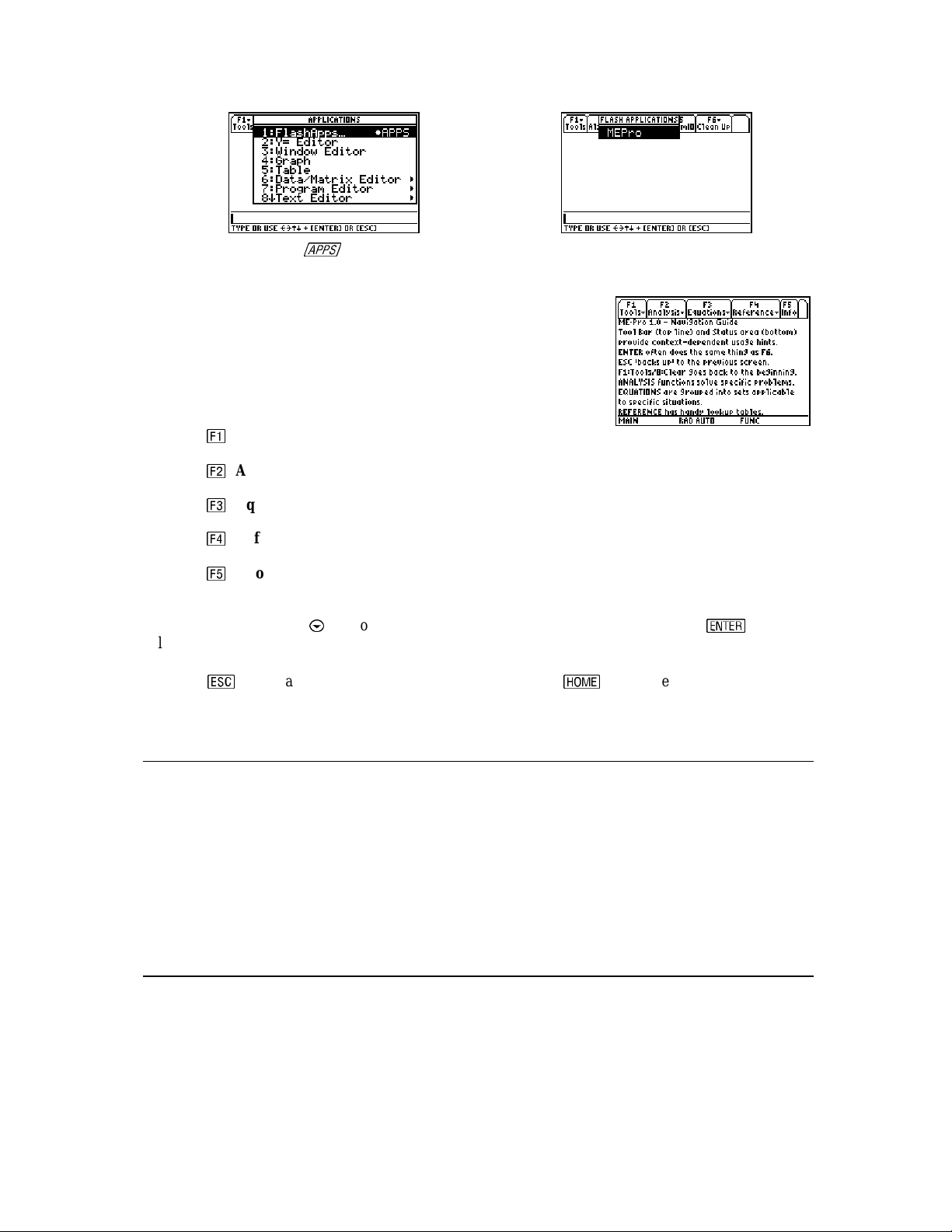
1.6 Starting ME••••Pro
To begin ME•Pro, start by pressing t he
move t he cu rsor bar to
press the
key to get to the home screen of ME•Pro. Alternatively, press
ME•Pro and press the
FlashApps...
key to get to the home screen of ME•Pro.
/
key. This accesses a pull down menu. Use the $ key to
. an d press
. Then move the highlight bar to ME•Pro and
/
; then, scroll to
ME⋅Pro for TI-89, TI-92 Plus
Chapter 1 - Introduction to ME-Pro
13
Page 14
Pull down Menu for
/
(FlashApps...option is at the top of the list)
Pull down Menu on for FlashApps...
(ME•Pro will be in the list)
The ME•Pro home screen is displayed to the right. The tool bar at the
top of the screen lists the titles of the main sections of ME•Pro which
can be activated by pressing the function keys.
b
: Tools: Editing features, information about ME•Pro in A: About.
c
: Analysis: Accesses the Analysis section of the software.
d
: Equations: Accesses the Equations section of the software.
e
: Reference: Accesses the Reference section of the software.
f
: Info: Helpful hints on ME•Pro.
To select a topic, use the $ ke y to mov e the highl i ght bar to the d e s ired top ic and pr e s s
, or
alternatively type the number next to the item. The Analysis, Equation and Reference menus are
organized in a menu tree of topics and sub-topics. The user can r eturn to a previous level of ME•Pro by
pressing . You can exi t ME•Pro at any time by pressing the
key. When ME•Pro is restarted ,
the software returns to its previous location in th e program.
1.7 How to use this Manual
The manual section, chapter heading and page number appear at the bottom of each page. The first chapter
in ea ch of the Analysis, Equations and Reference sections gives an overview of succeeding chapters and
introduces the navigation and computation features common to each of the main sections. For example,
Chapter 2 explains the basic layout of the Analysis section menu and the navigation principles, giving
examples of fe atu re s common to all topi cs in Analysis. Each topic in Analysis has a chapter dedicated to
describing its functionality in detail. The titles of these chapters correspond to the topic headings in the
software menus . They contain example problems and scr een di s p lays of the compu ted solut ions. Troubl eshooting information, commonly as ked questions , and a bibliograp hy use d to develop the sof tware a re
provided in appendixes.
1.8 Manual Disclaimer
The calculator screen displays in the manual were obtained during the testing stages of the software. Some
screen displays may appear slightly different due to final chan ges made in the software while the Manual
was being comple ted.
ME⋅Pro for TI-89, TI-92 Plus
Chapter 1 - Introduction to ME-Pro
14
Page 15

1.9 Summary
The designers of ME•Pro invite your comments by logging on to our website at http://www.dvtg.com or
by e-mail to improvements@dvtg.com
easy with the software by providing the following features:
• Easy-to-use, menu-based interface .
• Computational efficiency for speed and performance.
• Helpful-hints and context-sensitive information provided in the status line.
• Advanced ME analysis routines, equations, and reference tables.
• Comprehensive manual documentation for examples and quick reference.
. We hope that you agree we have made complex computations
ME⋅Pro for TI-89, TI-92 Plus
Chapter 1 - Introduction to ME-Pro
15
Page 16

Part I: Analysis
ME⋅Pro for TI-89, TI-92 Plus
Analysis -
16
Page 17

Chapter 2: Introduction to Analysis
2.1 Introduction
The analysis section contains subroutines and tools designed to perform specific calculations. Computations
include estimating thermodynamic properties of water at different temperature and pressure, in Steam
∆
Tables, computing fluid flow rates through different shaped orifices in Efflux, performing Wye to
conversions of AC circuits in EE for MEs, and evalueating cash flow for different projects in Capital
Budgeting. The computations are strictly top-down (i.e. the inputs and outputs are generally the same) and
the interface for each section guides the user through the solving process. A brief description of some of the
diff erent sections in Analys is appear below:
Steam Tables (3 sections): Saturated Steam, Superheated Steam, Air Properties computes the
thermodynamic parameters of steam including saturated pressure, enthalpy, entropy, internal energy, and
specific volume of the liquid and vapor forms of water given entri es of temperature and/or pressure. This
final topic covered computes the thermodynamic properties of dry air at different temperature s.
Thermocouples: This tool converts a specified tempe rature to an emf output in millivolts (mV) or from emf
output millivolts (mV) to a specified temperature. The software supports T, E, J, K, S, R and B type
thermocouples. These computation algor i t hms result from the IPTS -68 sta ndards adopted in 1968 and
modified in 1985.
circuit
Capital Budgeting: This section performs analysis of capital expenditure for a project and compares
projects against one another. Four measures of capital budgeting are included in thi s section: Payback
period (Payback); Net Present Value (NPV); Internal Rate of Return (IRR); and Profitability Index (PI).
This module provides the capability of entering, storing and editing capital expenditures for nine different
project s. Project s can be graph ed on NPV vs. k scale.
EE for Mechanical Engineers (3 sections): Performs e valuations on three types of circ u its: Impedance
↔∆
calculations; Circuit Performance; Wye
impedance admittance of a circuit consisting of a resistor, capacitor and inductor connected in Series or
Parallel. Performance parameters section computes load voltage and current, complex power delivered,
power factor, m axim u m power a va ilabl e to the l oad, a nd the load i mpedance req u ired t o receive the
maximum power from a single power source. The final segment of the software converts configurations
expressed as a Wye to its ∆∆∆∆ equivalent. It also performs the reverse computation.
Efflux (6 sections): Constant Liquid level; Varying liquid level; Conical Vessel; Horizontal Cylinder;
Large Rectangular Orifice; ASME Weirs (Rectangular notch; Triangular Weir; Suppres s ed Weir; Cipolletti
Weir) This section contai ns methods to compute fluid flow via cross sections of different shapes.
Section Properties (1 2 s ect ions): Rectangle; Hollow Rectangle; Circle; Circular Ring (Annulus); Uneven
I-section; Even I-section; C section; T section; Trapezoid; Polygon (n-s ided); Hollow P olygon (n-sided, side
thickness) Computes are a moment and location of center of mass for diff erent shaped cross sections.
Computed parameters inc lude the cross section area, the pol ar moment o f inertia, the area moment of inertia
and radius of gyration on x and y axes.
Hardness Number: A dimensionless number is a measure of the yield of a material from impact. Brinell
and Vicker developed two popular methods of measuring the Hardness number. These tests consist of
dropping a 10 mm ball of steel with a specified load such as 500 lbf and 3000 lbf. This steel ball results in
an indentation in the material. The diameter of indentation indicate s o f the hardness numbe r using e ither the
Brinell's or Vicker's formulation.
Circuit conversion
Impedance Calcula tions,
computes the
ME⋅Pro for TI -89, TI-92 Plus
Chapter 2- Introduction to Analysis
17
Page 18
2.2 Features of Analysis
Unit Management: Appropriate unit menus for appending units to variable entries or converting computed
results are accessible in most sections.
Numeric Computation – Variable entries must consist of real numbers (unless specified). Algebraic
expressions must consis t of defined variables so a numeri c val u e can be condensed upon entry.
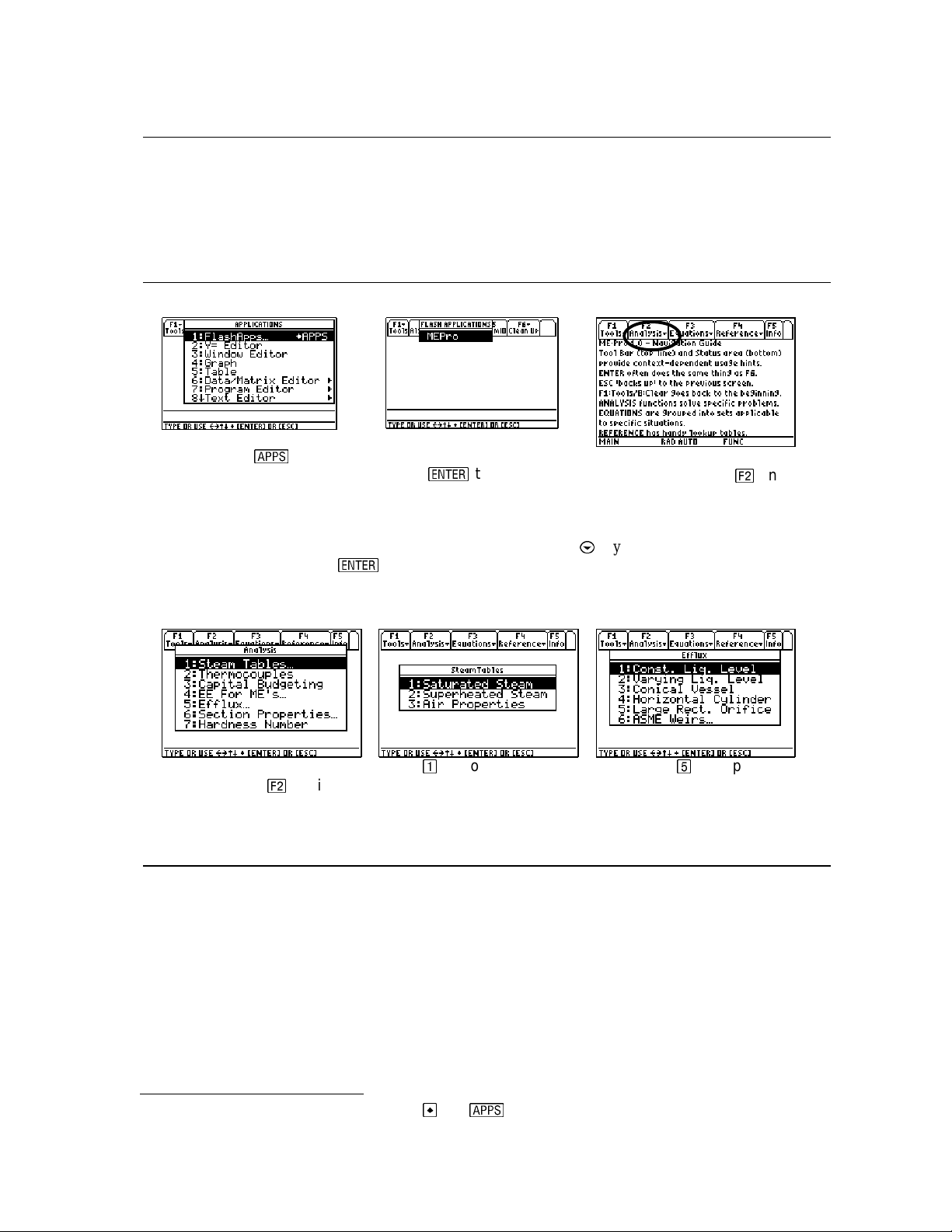
2.3 Finding Analysis
The following panels illustrate how to start ME•Pro and locate the
Analysis
section.
1. Press the
HOME screen to list the
applications stored in your
calculator.
There are seven sections under
desired heading and pressing
/
key in the
Analysis
2. Press 1:FlashApps and
press
to display the
applications stored in the
Flash section of memory.
1
3. HOME screen of ME
Analysis is listed as c on the
top function key row.
Pro.
•
. To sel ect a topic, use t he $ ke y to mov e the highl i ght bar to the
, or alternatively type the number next to the item to select. If a topic
contains several sections (Steam Tables, EE for MEs, Efflux, Section properties, an ellipsis (…) will appear
next to the title (see below).
From t he home screen of
ME•Pro
Press c
to display
Press for topics in
Tables
…
Steam
…or, press Z for topics in
Efflux.
the Analysis menu…
2.4 Solving a Problem in Analysis
The following example presents some of the navigational features in Analysis. This example is drawn from
Chapter 6: EE for MEs.
Problem - Calculate the performance parameters of a circuit consisting of a current source (10 - 5*i) with a
source admittance of .0025 - .0012*I, a load of .0012 + .0034*i. Display the real result of power in
kilowatts.
1
Steps 1 and 2 can be combined by pressing and
ME⋅Pro for TI -89, TI-92 Plus
Chapter 2- Introduction to Analysis
/
.
18
Page 19
1. From the home screen of
Pro, Press c to display
ME
•
the menu of Analysis.
4. While the cursor is
highlighting Load Type,
press the right arrow key,
or g to display the menu for
Load Type.
7. Variable descriptions
beginning with ‘Enter’ require
numeric entries.
2. Move the cursor to EE for
MEs and press
press Y).
5. In the menu for Load
Type move the cursor to
Admittance and press
.
(or
3. Select Circuit
Performance from the
submenu in EE for Mes.
6. Admittance is now
selected for Load Type and
the appropriate variables are
displayed.
8. Variable descriptions
beginning with the word
‘Resu lt’ are computed fields.
9. When entering a value,
press a function key to add
the appropriate units (c-h).
10. Following entry of all
input fields, pres s c: Solve to
compute the results.
13. To display a result in
different unit s , highlight the
variable and press f:Opts
move the cursor to 4
:Conv.
ME⋅Pro for TI -89, TI-92 Plus
Chapter 2- Introduction to Analysis
11. Results: Upper Half 12. Results: Lower Half
14. The unit menu for the
variable appears in the top
bar. Press t he func tion key
,
15. The computed value for
Real Power, P, is now displaye d
in kilowatts (kW).
corresponding to the desired
units.
19
Page 20
There are two types of interfaces in
Type 1: Input/Output/Choose Fields (Steam Tables, Thermocouples, EE for MEs, Efflux, Section
Properties, and Hardness Number). This input form lists the variables for which a numeric entry is required
and prompts the user to choose a calculation setting if applicable before computing the results. The entries
and results are always displayed in the same screen.
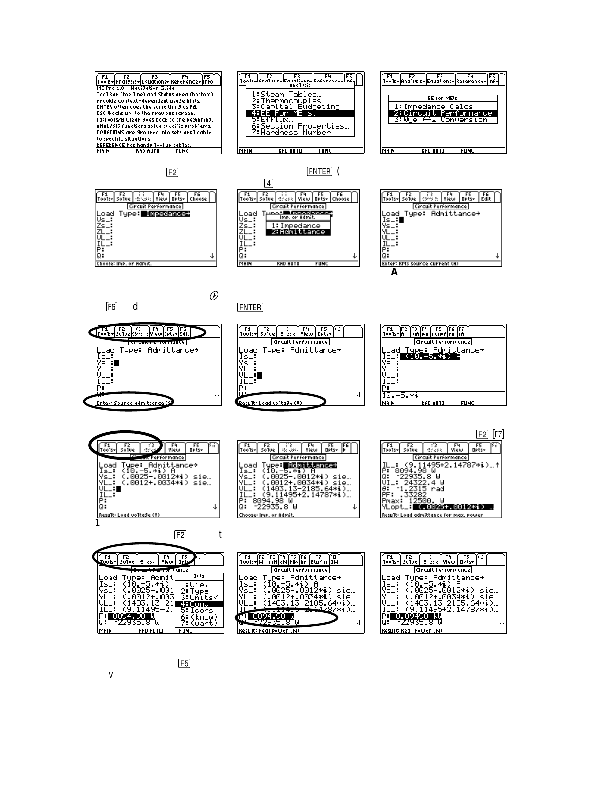
Type 2: Multiple Forms/Graphing (Capital Budgeting) This interface includes most of the features of
Type 1 with the additional screens used for entering cash flow for individual projects. The graphing
feat ures of t he calculator are enabled i n t his section for v i sualizing the rate of return (Net Present Value vs.
discount rate). An example of this interface is described briefly in this chapter, but in mor e detail in Chapter
5: Capital Budgeting.
Capital Budgeting
relevant data such as
displays below illustrate the basic user interface.
Input Screen for Capital
Budgeting
display Cash Flow for Project
1.
. Press e to
allows the user to compare relative financial performance of several projects with
Interest rate or discount rate (k), IRR, NPV, or Payback period. The screen
Analysis
A separate screen displays
the Cash Flow for ‘Project 1’.
Press c: Solve to r evert to
the previous screen.
:
Press d: Graph. Select ing
‘Multiple Graphs’
overlap of plots for different
projects (Projec t 1, Project 2,
etc.)
allows the
2.5 Tips for Analysis
The following instructions are useful in the Analysis section:
1. If an ellipsis (…) appears at the end of a menu title, a menu of subtopics exists i n this se ct i on .
2. An arrow ‘→→→→’ to the right of a heading, as in Load T ype, indicates an additional menu.
3. Variables ending with an underscore ‘_’, such as Vs_, Zs_, and IL_, allow complex values.
4. Descriptions for variables generally appear in the status line when the variable is highlighted.
5. Variables for which an entr y is required will have a description prefaced by the word ‘Enter’.
Computed variables begin with the word, ‘Result’.
To convert values from one unit to another, press
6.
th e variable at t h e top of the screen. Press the functio n key co rresponding to the appropriate units.
7. To return to the previous level of ME•Pro, press ..
8. To exit ME•Pro, press b: Tools and N: Clear.
9. To return to ME•Pro, p ress
10. To toggle between a graph and ME•Pro in split-screen mode, press
11. To remove the split screen in ME•Pro. 1) Press
Full Screen, 5)
: Save.
/
.
f:Opts, and 4:Conv to dis play the unit menu for
/
.
, 2) c: Page 2, 3) ": Split Screen App., 4) :
2.6 Function keys
Analysis
When
are s p ecific to the cont ex t of the section. Th ey are listed in Table 2-1:
functions are selected, the function keys in the tool bar access or activate features, which
ME⋅Pro for TI -89, TI-92 Plus
Chapter 2- Introduction to Analysis
20
Page 21
Table 2-1 Description of Analysis Function keys
Function Key Description
and
Tools
Solve
Graph
/
b
c
d
e
Labeled "
screen level. Th ese fu nctions are:
1: Open – This opens an existing folder to store or recall variables used in an
ME•Pro session.
2: (save as) – Not active in Analysis.
3: New – Creates a new folder for storing variable values used in an ME•Pro
session.
4: Cut - Removes entered values into the clipboard. Enabled for variables for
which t he user ca n enter va l u es.
5: Copy – Copies a highlighted value into the clipboard.
6: Paste – Pastes clipboard contents at cursor location.
7: Delete – Deletes highlighted values.
8: Clear – Return s to the HOME screen of ME•Pro.
9: (format)-Not active in Analysis.
A: About - Displays product name and version number.
Labeled "
selected problem and display any resulting output to the user.
Labeled "
be represent ed in graphical form. A gr aph can be viewed i n the full s creen or a
split screen mode. This can be performed by pressing
Normally labeled as "
cursor to be displayed using the entire screen in Pretty Print format.
In some cases @ is labeled as "Pict", "Cash".
"Pict" is available in the Section Properties or Hardness Number sections
and when selected displays a diagram to facilitate better understanding of the
problem.
"Cash" is used in Capital Budgeting section of the software.
Labeled "Opts" - Thi s key displays a po p up me nu l i s ting the options:
1: View - allows the highlighted item to be viewed using Pretty Print.
2: (type) - Not active
3: Units – This activates, or deactivates the unit management feature.
4: Conv – Displays the unit menu for the highlighted variable and allows the
conversion of an entry or result into different units.
5: Icons - Presents a dialog box identifying certain Icons used by the software to
display content and context of the information. These icon systems are only used
in equ a t ions.
6: (know)- Not active
7: Want - Not active
“Edit” - Brings in a data entry line for the highlighted parameter.
“Choose” in Capital Budg et ing enables th e user to select from one of n ine
project s.
“√ Check” requesting the user to press this k ey to select a highlighted parameter for
use in an Analysis computation.
"Add” Adds a cash flow entr y for a project in Ca pital Budget ing section.
(Not active)
" - displays all the functions available on the TI-89 at the Home
" - Pressing this key enables the software to begin solving a
" - This feature is available in input scree ns where the solution can
followed by c. Use
to toggle between the data entry screen and graph window.
View
" - This enables the information highlighted b y the
ME⋅Pro for TI -89, TI-92 Plus
Chapter 2- Introduction to Analysis
21
Page 22

2.7 Session Folders, Variable Names
ME•Pro automatically stores its variables in the current folder specified by the user in
screen. The cur rent folder name is displayed in th e lower left corner of th e s creen (default is “Main”). To
create a new folder to store values for a particular session of ME•Pro, press :/TOOLS, :/NEW and
type t he nam e of the new folder (see Gu idebook for the com plete det ail s of crea ting and m anaging fol ders;
Chapter 5 for the TI-89 and Chapter 10 for the TI-92 Plus).
There are several ways to display or recall a value:
• The conten ts of variables in any folder can be d ispla yed using
variable name and pressing to display the contents of a particular variable.
• Variables in a current folder can be recalled in the HOME screen by typing the variable name.
• All inputs and calculated results from the Analysis and Equations section are saved as variable
names. Previously cal culat ed , or enter ed values for va ria bl es in a fold er are rep laced wh en
equatio ns are solved using new values for inputs.
or the HOME
, moving the cursor to the
2.8 O verwriting of variable values in graphing
When an equation or analysis function is graphed, ME•Pro creates a function for the TI grapher, which
expresses the dependent variable in terms of the independent variable. This function is stored under the
variable name pro (x). When ME•Pro’s equation grapher is execute d , v alu es are inserted into the
independent variable for pro (x) an d va lues for the dependen t value ar e calcul ated. Whatever val u es
previously existed in either of the dependent and independent variables in the current folder are cleared. To
preserve data under variable names, which may conflict with ME•Pro’s variables, run ME•Pro in a separate
folder.
2.9 Reserved Variables
A list of reserved variable names used by the TI operating system, which cannot be used as user variable
names or entries are listed in Appendix F.
ME⋅Pro
for TI -89, TI-92 Plus
Chapter 2- Introduction to Analysis
22
Page 23

F2: Analysis/1: Steam Tables
Chapter 3: Steam Tables
Steam properties are a complex function of temperature, pressure, volume, critical temperature, critical
pressure, and molecular weight of water. Our software takes into account the ranges of temperature and
pressure that results in good fits to data gathered over a long periods in many parts of the world.
Steam Tables offer a collectio n of programs organized as a powerful computational engine to calculate
thermodynamic properties of steam in a user-friendly environment. Calculations of thermodynamic
properties are based on standards and conventions adopted by the International Conventi ons covering
properties of saturated and superheated steam.
3.1 Saturated Steam Properties
This section computes the properties of saturated steam at a single temperature or pressure.
Variable Description Units
Ps Saturation pressure MPa
Ts Saturation temperature K
Vf Specific volume – liquid m3/kg
Vg Specific volume – vapor m3/kg
Hf Enthalpy – liquid kJ/kg
Hfg Latent heat of vaporization kJ/kg
Hg Enthalpy – vapor kJ/kg
Sf Entropy – liquid
Sfg S (g) - S (f)
Sg Entropy – vapor
UF Internal energy – liquid
UG Internal energy – vapor
kJ/(kg⋅K)
kJ/(kg⋅K)
kJ/(kg⋅K)
kJ/(kg⋅K)
kJ/(kg⋅K)
3.2 Superheated Steam Properties
The properties of superheated steam require two inputs: temperature and pressure. From the data suppli ed ,
the program will compute saturated temperature, specific volume, enth alpy and entropy. The data is
displayed in a tabular form.
Variable Description Units
Temp Given temperature K
Sat Pressure Given pressure MPa
Sat Temperature Corresponding temperature K
Specific Volume Specific volume m3/kg
Enthalpy Enthalpy kJ/kg
Entropy Entropy
kJ/(kg⋅K)
3.3 Air Properties
The properties of dry air are computed using the ideal gas law model as the basis. Using temperature as a n
input, the softwa re computes a var iety of parameters including specific heats, enthalpy, entrop y, and
velocity of sound.
Variable Description Units
Temp Given temperature K
CP Specific heat at constant pressure
J/(kg⋅K)
ME⋅Pro for TI -89, TI-92 Plus
Chapter 3 - Analysis – Steam Tables
23
Page 24
F2: Analysis/1: Steam Tables
Variable Description Units
CV Specific heat at constant volume
H Enthalpy J/kg
U Internal energy J/kg
E Entropy function
IPR Isentropic pressure function unitless
IVR Isentropic volume function unitless
G Specific heat ratio unitless
A Speed of sound m/s
J/(kg⋅K)
J/(kg⋅K)
3.4 Using Steam T ables
Once you have selected STEAM TABLES at the main menu, the first screen displays three subtopics Saturated steam, Superheated steam and Air properties. Selecting “saturated steam properties”, allows
properti es t o be calcula ted from u ser- entered value of t emperature or pressure. However, p roperties for
“superheated steam” req uire v a lues for both tempe ra t ure and pressure. Thermodyna mic properties of air are
calculated for dry air conditions only.
Example 3.1:
Calculate the properties of saturated steam at 130 °C.
Solution - Select the Saturated S team section. The input screen calls for defining known parameter
(temperature o r pressure) . The default condition is temperature. Move the pointer to the next line and start
entering the temperature. The function keys assume unit assignments for the data about to be entered. For
our example, enter 130 an d press ? key thereby attaching °C to the value just entered. Press > to solve
for the thermodynamic parameters.
Upper Display Lower Display
All the calculated parameters are displayed on the screen w ith SI units attached as shown. If you desire to
see the value of saturated pressure parameter Ps, use the ke y to mov e the highl i gh t bar to capture Ps.
Press A to display a pull down menu of items to select. Select 4 (Conv). This allows other units for Ps
such as Pa, kPa, atm, psi, torr attached to ?, @, A, B, and C respect ively. Pres sing B converts the
value of Ps into the new units of psi. The display is refreshed immediately in the units just selected.
Example 3.2:
Calculate the properties of superheated steam at 125 °C and 20 psi.
Solution - Select the Supe rhea ted Steam se ction. The input screen calls for e ntering temperat ure and
pressure. Move the pointer to enter the 125 °C and 20 psi for temperature and pressure. Make sure that the
appropriate units are attached to the data using the function keys. Press > to solve for the thermodynamic
parameters.
ME⋅Pro for TI -89, TI-92 Plus
Chapter 3 - Analysis – Steam Tables
24
Page 25
F2: Analysis/1: Steam Tables
Upper Display Lower Display
All the calculated parameters are displayed on the screen with units attached as shown. The displayed
results could be converted to other un its as described in the first example described earlier.
Example 3.3:
Calculate the properties of dry air to be -20 °C.
Select the Air Properties section. The input screen calls for defining the temperature. Enter a temperature
of – 20 °C. When ent erin g -20 °C, be sure to u se the unary operat or key followed by 20 °C. If you
use\ key fo r a negative value this will result in an input error.
Press > to solve for the thermodynamic properties of air.
Input Screen Result screen
All the calculated parameters are displayed on the screen with SI units attached as shown. The parameters
computed can be viewed in other units as described in the examples shown here.
3.5 Validity Range for Temperature and Pressure
The computed results are valid only for the following finite ranges of temperature and pressure:
Saturated Superheated
Temperature: 273.16 - 647.3 K Saturated temperature
Pressure: 0.006113 - 22.08 MPa Pressure: 0.006113 - 22.08 MPa
References:
1. Lester Haar, John S. Gallagher and George S. Kell, NBS/NRC Steam Tables, Thermodynamic and
Transport Properties for Vapor and Liquid States of Water, Hemisphere Publishing Corporation,
Washington, DC.
2. Steam Tables, 1967; Thermodynamic properties of Water a nd Steam, The Electric Research Association,
Edward Arnold Limited, London England, 1967
3. Th omas F. Levine, Jr., and Peter E. Liley, Steam and Gas Tables with Computer Equations, Academic
Press, New York, NY, 1984
ME⋅Pro for TI -89, TI-92 Plus
Chapter 3 - Analysis – Steam Tables
25
Page 26
F2: Analysis/ 2: Thermocouples
Chapter 4: Thermocouples
This chapter describes using the software in the Thermocouples menu. Thermocouple parameters are
calculated for the class of thermocoupl es in comm on usa g e.
4.1 Introduction
This tool c onverts a specified temperature to an emf output, millivolts (mV), and from an emf output,
millivolts (mV), to a specified temperatur e. The software supports Type T, E, J, K , S, R and B
thermocouples. The underlying assumption is a reference t emperature of 0 °C. These computation algorithms
result from the IPTS-68 standards adopted in 1968 and modified in 1985.
4.2 Using the Thermocouples Function
Select the Thermocouples function from the Analysis menu by highlightin g Thermocouples an d pressing
¸
. This action brings out the main use r inte rf ace scre en. Press B to view the choices availabl e. Seven
types of T hermocou ples a re a vail able for com putations. For example, to sele c t a Pt-10%Rh-Pt thermocoup l e
referr ed to as S Type ther mocouple, move the hi g h th e highlight bar to Type S and press
At this point, the software presents the primary user interface awaiting data entry. At the same time, the
mat erial of the ther mocouple a nd the vali d ran g e are displa yed for reference.
¸
or press z.
Thermocouple computations involve computing emf available from a known temperature or computing a
temperature from an emf. The latter case is by its very nature not as accurate as the first type of computation.
Screen 1 (for temperature) Screen 2 (for emf)
Example 4.2:
Find the emf for an S type thermocouple at 400 °F. From the value of emf computed, compute t he
temperature.
Solution 4.2:
Select Type S thermocouple for t his problem. For temperature, enter 400, t hen press …. The computed emf
is 1.4777mV. Now return t o Kn own line and select emf for input. Ent er 1.4777 mV for emf to get 403.989 °F
for temperature.
Notes: Th e ther mocouple em f ca lcula tion can be ex p anded t o cover the em f produced by th e thermocouple if
the reference temp erat ure was di fferent from 0 °C. For example, if t he reference t emperature was 30 °C
instead of 0 °C, you compute the resulting emf in two steps; first find the emf (emf 1) for the temperature
desired, say 300 °C, and the emf (emf 0) for the reference temperature. The resulting emf for the new
refer ence temperature of 30 °C is the difference between the two emf’ s, i.e., "em f 1 - emf 0".
ME⋅Pro for TI-89, TI-92Plus
Chapter 4 - Analysis - Thermocouples
26
Page 27

F2: Analysis/ 2: Thermocouples
4.3 Basis for Temperature/Voltage Conversions
The temperature-to-voltage conversion is based on either a polynomial approximation or a combination of a
polynomial coupled with a special sequence. This ensures precise calculations within some prescribed error
range. These rages a re displayed on each inpu t screen.
References:
1. Robert L. Powell, William J. Hall, Clyde H. Hyink, Larry L. Sparks, George W. Burns, Margaret Scoger
and Harmon H. Plumb, Thermocouple Reference Tables based on IPTS-68, NBS Monograph 125, Omega
Press, 1975
ME⋅Pro for TI-89, TI-92Plus
Chapter 4 - Analysis - Thermocouples
27
Page 28

F2: Analysis/3: Capital Budgeting
Chapter 5: Capital Budgeting
This chapter covers the four basic measures of capital budgeting:
♦ Payback Period ♦ Internal Rate of Return
♦ Net Present Value ♦ Profitability Index
5.1 Using Capital Budgeting
This section performs analysis of capital expenditure for a project and compares projects against one another.
Four measures of capital budgeting are included in this section: Payback period (Payback); Net Present Value
(NPV); Internal Rate of Return (IRR); and Profitability Index (PI). This module provides the capability of
entering, storing and editing capital expenditures for nine different projects. The following equations are used
in calculations:
n
CF
()1
t
−
CF
t
=
t
+
k
0
Eq. 1
NPV
=
∑
t
=
1
n
CF
+
n
∑
t
=
t
IRR
()1
1
∑
t
=
PI
()1
1
=
CF
CFt: Cash Flow at time t.
Payback: The number of time periods it take s a fir m to re cover its original invest ment.
NPV: The present values of all future cash flows, discounted at the selected rate, minus the cost of the
investment.
IRR: The discount rate that equates the present value of expected cash flows to the initial co st of the proj ect.
PI: The present va lue of the future cash flows, discounted at the selected rate, over the initial cash outlay.
CF
−=
t
=
0
t
CF
+
t
=
t
t
k
0
0
Eq. 2
Eq. 3
ME⋅Pro for TI-89, TI-92 Plus
Chapter 5 - Analysis - Capital Budgeting
28
Page 29
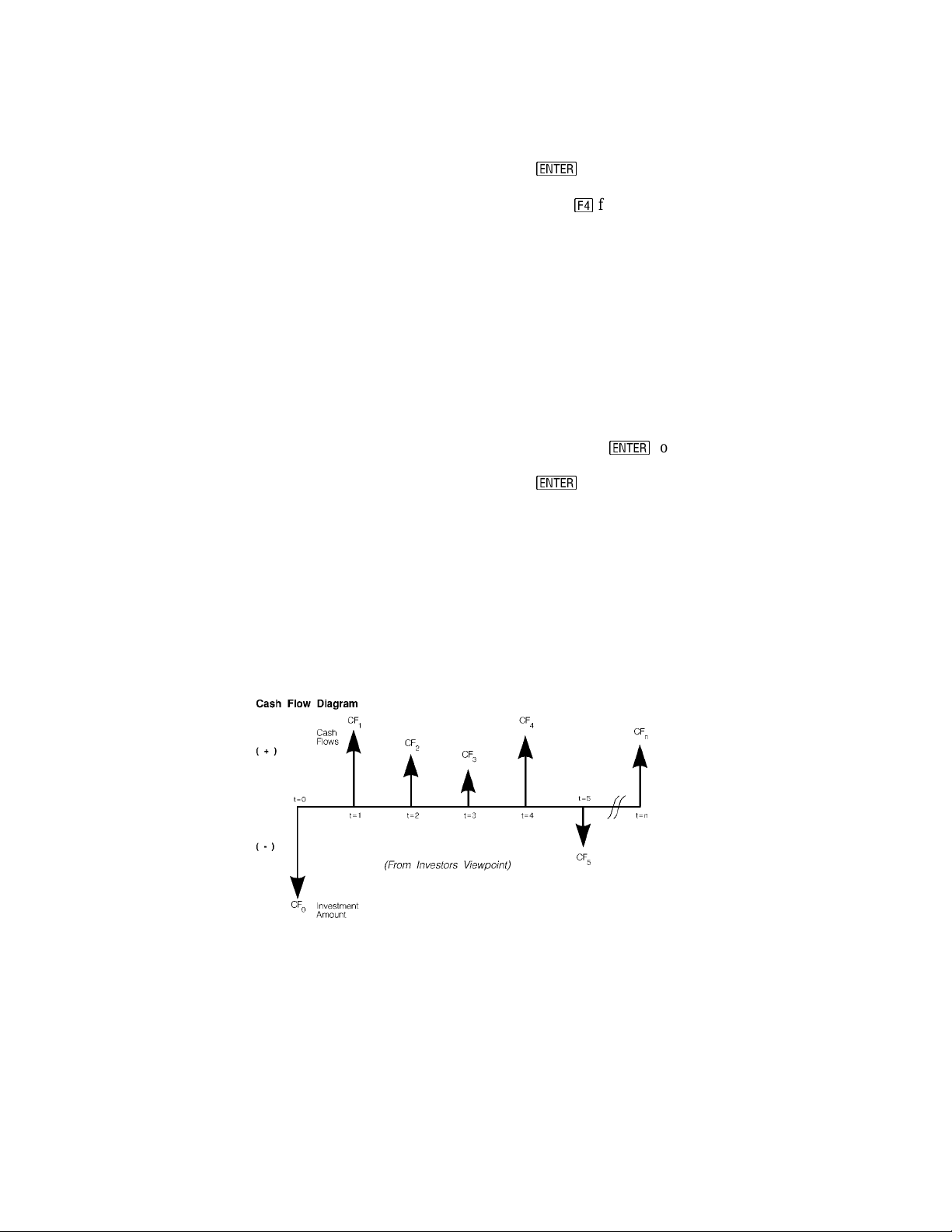
F2: Analysis/3: Capital Budgeting
Field Descripti ons - Input Screen
Project:
k:
Payback:
npv:
IRR:
PI:
Multiple
Graphs
Full
Screen
Graph
NAME:
t0:
t1:
tn:
(Project)
Press
to select one of nine unique
projects or edit the current name of the project
by pressing e for Cash option.
(Discount Rate per Period in %) Enter a real number.
(Payback Period) Returns a real number.
(Net Present Value) Returns a real number.
(Internal Rate of Return) Returns a real number (%).
(Profitability Index) Returns a real number.
(Graph multiple projects
simultaneously)
(Graph on full or split screen?) Press
Activation of this feature enables the overlay
of each success i ve gr a p h (pr oject s) on t he
Press
same axis.
to activate.
to activate.
Field Descriptions - Project Edi t Screen
(Project Name) Enter the name of the project.
(Investment at t=0) Enter a real number.
(Cash flow at t=1) Enter a positive or negative real number.
(Cash flow at t=n) Enter a positive or negative real number.
Example 5.1:
The following projects have been proposed by ACME Consolidated Inc. What are t he Payback period, Net
Present Value, Internal Rate of Return, and Profitability Index of each project? Which is the more viable
project?
ME⋅Pro for TI-89, TI-92 Plus
Chapter 5 - Analysis - Capital Budgeting
29
Page 30
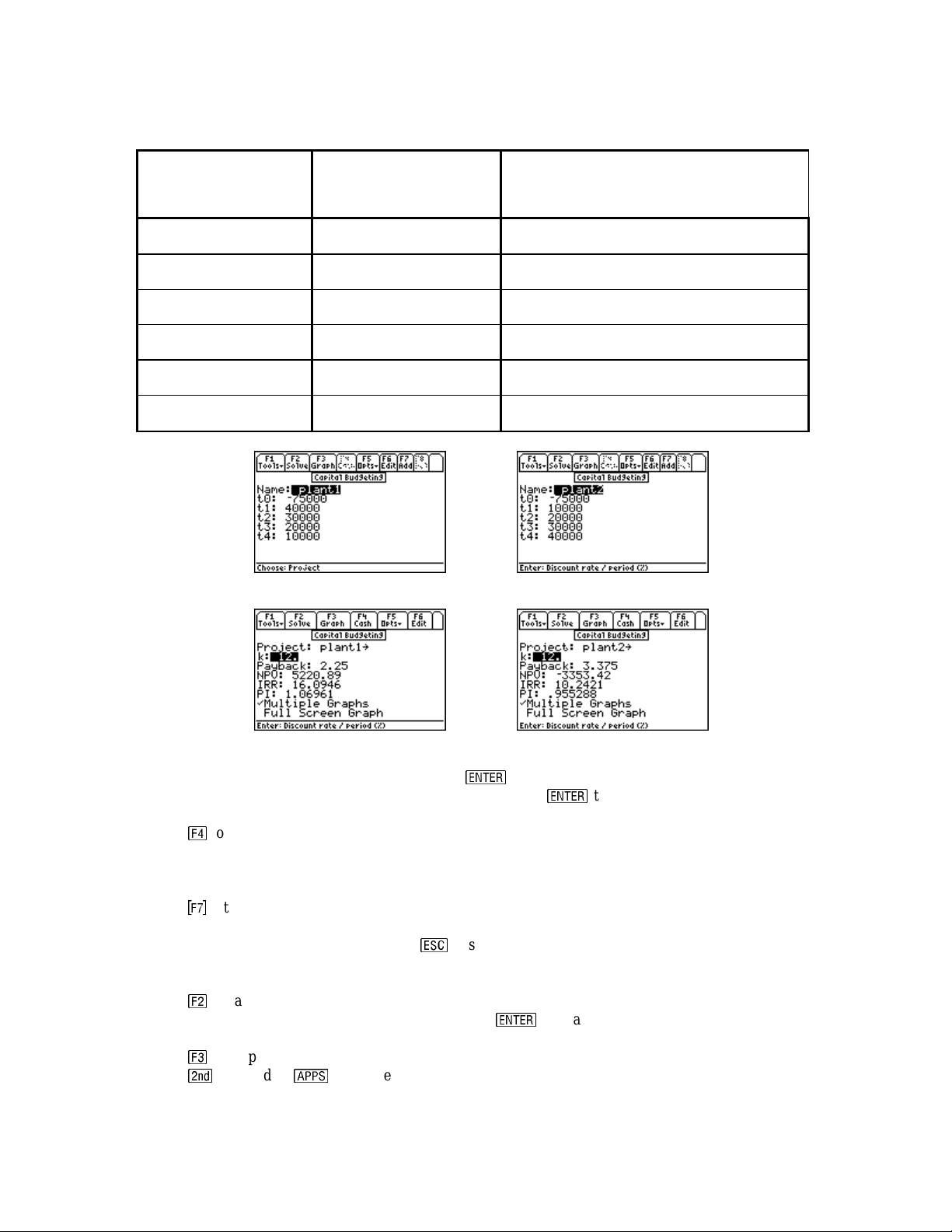
Table 5-1 Cash Flow for two projects
Name of Project: Plant 1 Plant 2
Investment Outlay:
$75,000 (at t=0) $75,000 (at t =0)
Cost of Capital: 12% 12%
Year Net Cash Flow ($) Net Cash Flow ($)
0 -75,000 -75,000
1 40,000 10,000
2 30,000 20,000
3 20,000 30,000
4 10,000 40,000
F2: Analysis/3: Capital Budgeting
Cash Flow Input: plant1 Cash Flow Input: plant2
Output Scr een: plant1
Output Scr een: plant2
1. With the highlight bar on the Project field, press
not been used. Note: this example uses projects 1 and 2. Press
to select a project to edit. Select a project that has
to return to the Capital Budgeting
screen.
2. Press e to select Cash option; enter the project edit screen; and, edit the cash flows.
3. Enter “plant1” in the Name field. Note: Cash flo w data for this proj ect will be sto r ed in a variable of thi s
name. Therefore the entered name must begin with a letter; be no more than 8 characters in length; and,
contain no embedded spaces.
4. Press h 5 times to add 5 time points and enter the cash flows at each time point from the table on the
pr e vious page. W hen finished, your s c reen shoul d look like the projec t edi t screen above. Be s ure to en ter
75,000 as a negative number for t0. Press . to save your changes and return to the Capital Budgeting
screen.
5. Enter 12 for k.
6. Press c to calculate Payback, NPV, IRR, and PI.
7. Move the highlight bar to Multiple Graphs and press
to en able overlayin g of succes s ive grap hs of
each p roject.
8. Press d to graph the curvilinear relationshi p between the Net Present Value and the Discount Rate.
9. Press followed by
/
to enable the graph editing toolbar.
ME⋅Pro for TI-89, TI-92 Plus
Chapter 5 - Analysis - Capital Budgeting
30
Page 31

F2: Analysis/3: Capital Budgeting
10. T he cur ve i ndicates where k=0, the Net Present Value is simply cash inflows minus cash outflows. The IR R
% is sho wn at the point where NPV=0. Using the built-in graphing capabilities o f the TI 89, you can trace the
graph to find the values of these two points. The TI 89 will give you the exact coordinates of any point along
the graph. Press followed by
/
to return to the Capital Budgeting screen.
11. Repeating steps 1 through 9 for the second project, under the Project field, “plant2” and input the values in
Table 5-1. Activating the Multiple Graph feature enables a simultaneous plot of the two projects. This will
overlay a second graph on top of a previously plotted function. First plot plant1. After gr ap hing, plot plant2.
The first cu rve to ap p ear, is plant1, the second is plant2. The most viable project in terms of discounted cash
flows, in this example, is the one with the highest curve.
12. Pressing
c "
resets the display to full screen.
Plot of Project 1 Overlay of Project 2
ME⋅Pro for TI-89, TI-92 Plus
Chapter 5 - Analysis - Capital Budgeting
31
Page 32

F2: Analysis/4: EE for ME’s
Chapter 6: EE for Mechanical Engineers
This chapter describes the software in the AC Circuits section and is organized under three topics. These
topics for m the backbo ne of circuit calcu lations of interes t to mechanical en gine e rs.
♦ Impedance Calculations ♦ Circuit Performance
♦ Wye ↔ ∆ Conversion
6.1 Impedance Calculations
Impedance Calculations
The
resistor, capacitor and inductor connected in Series or Parallel. The impedance and admittance values are
displayed to the user in r eal or complex form.
topic computes the impedance and admittance of a circuit consisting of a
Field Descripti ons
CONFIG:
Elements:
fr:
R:
L:
C:
ZZ_:
YY_:
Circuit Configuration
Element Combination
Frequency in Hz
Resista n ce in ohms; only
appears if RL, RC or RLC is
chosen in Elements field
Inductance in Henry; only
appears if L, RL, LC or RLC is
chosen in Elements field
Capacitance in Farads; only
appears if C, LC, RC or RLC is
chosen in Elements field
Impedance in ohms
Admittance in Siemens
(Press
_
_
and select Series or Parallel
__
configuration by usin g
_
to display the input screen updated for the new
configuration..
Press
_
_
to display the following circuit elements:
__
L, C, RL, RC , LC an d RLC T he choice of elements
determines which of the input fields are available.
Enter a real positive number.
Enter a real positive number.
Enter a real positive number.
Enter a real positive number.
Returns a real or co mp lex number.
Returns a real or comp lex number.
. After choosing, press
Example 6.1:
Compute the impedance of a series RLC circuit consisting of a 10-ohm resistor, a 1.5 Henry inductor and a
4.7 Farad capacitor at a frequency of 100 Hz.
ME⋅Pro for TI-89, TI-92 Plus
Chapter 6 - Analysis - EE for MEs
32
Page 33

F2: Analysis/4: EE for ME’s
Input Screen Output Scr een
1. Choose Series for Config and RLC for Elements using th e proce dur e described a bove .
2. Enter 100 Hz for Freq.
3. Enter 10 Ω for R; 1.5 Henry for L; a nd 4.7 F for C.
4. Press
>>>>
to calculate ZZ_ and YY_
.
5. Th e output screen shows the results of computation.
6.2 Ci rcuit Performance
This section shows how to compute the circuit performance of a simple load connected to a voltage or cur rent
source. Perform ance parameters include load voltage and current, complex power delivered, power factor,
maximum p ower available to the load, and the load impeda nce required to receive the maximum power .
Field Descriptions - Input Screen
Load Type:
Vs_:
Zs_
ZL_:
Type of Load Press
rms Source Voltage in V A real or complex number.
Source Impedance in
Ω
Load Impedance in
Ω
_
_
to select load impeda nce (Z) or
__
admittance (Y). This w ill de te rmine whether the
remaining fields Vs_, Zs_, and ZL_ or Is_, Ys_,
and YL_ are di s p layed, respecti vel y.
A real or complex number.
A real or complex number.
Is_:
ys_:
yl_:
Vl_:
il_:
P:
Q:
ME⋅Pro for TI-89, TI-92 Plus
Chapter 6 - Analysis - EE for MEs
rms Source Current in A
Source Admittance in Siemens Enter a real or complex number.
Load Admittance in Siemens Enter a real or complex number.
Load Voltage in V Returns a real, complex number.
Load Current in A Returns a real, complex number.
Real Power in W Return s a real number.
Reactive Power in W Returns a real number.
A real or complex number.
Field Descriptions - Output Screen
33
Page 34

F2: Analysis/4: EE for ME’s
VI_:
θθθθ:
Apparent Power in W Returns a complex number.
Power factor Angle in degrees
Returns a real numbe r.
or radian, determined by the
setting
PF:
Pmax:
Zlopt_:
Load Power Factor Returns a real number.
Maximum Power Available in W Returns a real number.
Load Impedance for Maximum
Power in
Ω
- if Impedance is
Returns a real, complex number.
chosen for Load Type at the
input screen
Ylopt_:
Load Admittance for Maximum
Returns a real, complex number.
Power in Siemens - if
Admittance, is chosen for Load
Type at the input screen
Example 6.2:
Calculate the performance parameters of a circuit consisting of a current source (10 - 5*i) with a source
admittance of .0025 - .0012* I, and a load of .0012 + .0034*i.
Input Screen Output: Upper Half Output: Lower Half
1. Ch oose Admittance for Load Type.
2. En ter th e value 10 - 5*i A for
Is_.
3. Enter t he value .0025 - .0012* i siemens for Ys_, and .0012 + .0034* i siemens for a load of YL_.
4. Press ? to calculate the performance parameters.
5. The input and result s of computa tion are shown above.
6.3 Wye ↔↔↔↔ ∆∆∆∆ Conversion
The Wye ↔ ∆ Conversion converts three impedances connected in Wye or ∆ form to its corresponding ∆ or
Wye form, i.e., Wye ↔ ∆ or ∆ ↔ Wye
Input Fi elds -
Input Type: Selecti on ch oi ces a re ∆→Wye or Wye→∆. This
determines whether the next 3 fields (input fields)
accept ∆ or Wye Impedances.
ZZA_:
ZZB_:
ZZC_:
∆
Impedance Real or complex number.
∆
Impedance Real or complex number.
∆
Impedance Real or complex number.
. Fig. 6.1 Wye Network
ZZ1_: Y Impedance Real or complex number.
ZZ2_: Y Impedance Real or complex number.
Z3
Z1
Z2
ME⋅Pro for TI-89, TI-92 Plus
Chapter 6 - Analysis - EE for MEs
34
Page 35

F2: Analysis/4: EE for ME’s
ZZ3_: Y Impedance Real or complex number.
Result Fields
ZZA_: (
ZZB_: (
ZZC_: (
∆
Impedance) Real or complex number.
∆
Impedance) Real or complex number.
∆
Impedance) Real or complex number.
ZZ1_: (Y Impedance) Real or complex number.
ZZ2_: (Y Impedance) Real or complex number.
ZZ3_: (Y Impedance) Real or complex number.
Fig. 6-2 ∆∆∆∆ Network
ZB
ZC
Example 6.3:
ZA
Compute th e Wye im p edance eq uivalent of a ∆ network with impedances
75+12*i, 75-12*i, and 125 ohms.
1. Select ∆ →Y for Input Type. .
2. Enter the values 75+12*i
3. Press
>>>>
to calculate ZZ1_, ZZ2_ and ZZ3_.
Ω
, 75 -12*i Ω, 125 Ω for ZZA_, ZZB_ and ZZC_ respectively.
Input Parameters Calculated Output
Ω
The computed results are: ZZ1_: 34.0909 - 5.45455⋅ i
ZZ2_: 34.0909 + 5.45455⋅ i
Ω
ZZ3_: 20.9782
Ω
References:
1. Sanford I. Heisler, The Wiley Engineer's Desk Referen ce, A concise gu ide for t he Pr ofessional Engineer, John
Wiley and Sons, New York, NY, 1984
2. James W. Nilsson, Electric Circuits, 2nd Edition, Addison -Wesley Publishing Company, Reading MA, 1987
and later editions.
ME⋅Pro for TI-89, TI-92 Plus
Chapter 6 - Analysis - EE for MEs
35
Page 36

F2: Analysis/5: Efflux
Chapter 7: Efflux
This section of Analysis contains methods to compute fluid flow via cross sections of different shapes.
Many of th e s e formula s have been d e rived empirically over many years of ex perimental observations.
♦ Constant Liquid Level ♦ Varying Liquid Level ♦ Conical Vessel ♦ Horizontal Cylinder ♦ ASME Weirs
7.1 Constant Liquid Level
This portion of the software computes fluid discharge from an opening of cross sectional area So (m2),
and a constant head H (m). The discharge coefficient αααα (unitless) is a unique number (a number less than
1) accounting for t he sh ape of the cross section, edge-rounding effects, an d turbu lence effects. Upon
receivi ng these inputs, th e s oftwa re computes the volume d ischa rge, Q, (m
V (m/s).
Example 7.1:
Find the discharge parameters for a 1.5 sqft opening subject to a head of 4_m. Assume the discharge
coefficient to be 0.85.
3
/s) and the discharge velocity
Input Screen Result Screen
2
To solve the pr oblem, en ter va lues for αααα = 0.85, H = 4 m and so = 1.5 ft
using the appropriate unit keys
acce ssible during data entry. After all the input variables have been entered, press ? key to get the
following results.
Given: Results
α = 0.85
So = 1.5 ft
H = 4 m
2
V = 7.52877 m/s
Q = 1.04917 m
3
/s
7.2 Varying Liquid Level
This segment of the software considers fluid discharge from a tank of cross sectional area S (m2), an
opening of cross sectional area So (m
dischar g e coefficient αααα (unitless) is a unique number (a number less than 1) accounting for the shape of
the cross sectio n, edge-rounding effects, and t urbul ence effects. Upon receiving t hese i nput s , th e
software computes the time t (s) taken t o see the drop in head heig h t .
Example 7.2:
A large reservoir has an area of 10000 m
2
The drainage opening is 3 m
and has a discharge coefficient of 0.95. How long will this process take?
2
) where the head has dropped from H1 (m) to H2 (m). The
2
ha s hea d level of 4_m that need s to brought down by 0.5_m.
ME⋅Pro for TI-89, TI-92 Plus
Chapter 7 - Analysis - Efflux
36
Page 37

F2: Analysis/5: Efflux
Input Screen Result Screen
2
To solve the pr oblem, en ter va lues for αααα = 0.95, H1 = 4 m, H2 = 3.5 m and So = 3 m
using the
appropriate unit keys accessible when data is being entered. After all the input variables have been
entered, press ? key to get the results.
Given: Results
α = 0.95
S = 10000 m
So = 3 m
2
H1 = 4 m
H2 = 3.5 m
2
t = 204.68 s
7.3 Conical Vessel
This segment considers fluid discha rge from a container that conical in shape. The parameters specified
for the computations include cross sectional area, So (m
fluid head at t. The discharge coefficient αααα (unitless) is a unique number (a number less than 1)
accoun ting for the shape of the cross sectio n, edge-rounding effects, turbu lent effect s , an d ββββ (rad) refers
to th e cone an gle. Upon receiving these inpu ts, the software computes the time for the head to \drop from
H1 to H2.
Example 7.3:
Find the time taken to dis charge water fro m a 25 ° conical vessel with a disch arge coeff icient of 0.95 for a
2
1.2 cm
opening. Consider the head drops from 24 in to 18 in. The base of the cone has a diameter Dl of
12 in.
2
), and a fluid head H1 (m) at t=0 and H2 (m) the
Input Screen Result Screen
2
To solve the pr oblem, en ter va lues for αααα = 0.95, H1 = 24 in, H2 =18 in, and So = 1.2 cm
using the
appropriate unit keys accessible when data is being entered. After all the input variables have been
entered, press [F2] key to get the results.
Given: Results
α = 0.95
So = 1.2 cm
2
t = 121.456 s
Dl = 12 in
H1 = 24 in
H2 = 18 in
β = 25 deg
ME⋅Pro for TI-89, TI-92 Plus
Chapter 7 - Analysis - Efflux
37
Page 38

F2: Analysis/5: Efflux
7.4 Horizontal Cylinder
This segment of the software computes fluid discharge from a cylindrical tank of diameter D (m) and
length L (m). The parameters specified for the computations include an opening for di scharge with an
area So (m
coefficient αααα (unitless) is a unique number (a number less than 1) accounting for the shape of the cross
section, edge-rounding effects, a nd turbulent effects, along with Ks (unitless), and a space factor
coefficient.
Example 7.4:
Find the time to oil from a cylindrical tank 12 m in diameter and 20 m long vessel with a space factor of
0.8 and orifice discharge coefficient of 0.75. How long does it take f or the oil to drop down 10 cm from
an initial height of 5 m. Assume the orifice opening to be 1.2 mm
2
), and a fluid head H1 (m) at t=0 and H2 (m) the fluid head at t. In addition, the discharge
2
.
Input Screen Result Screen
To solve the pr oblem, en ter va lues for αααα = 0.55, Ks = 0.8 m, H1 = 5 m, H2 = 3.5 m, L = 20 m, and So =
2
1.2 cm
using the appropriate unit keys accessible when data is being entered. After all the input
vari ables ha ve been entered, pres s ? key to get the results.
Given: Results
α = 0.75
Q = .090698 _m^3/s
H1 = 5 m t = 492061 s
H2 = 4.9 m
L = 20 m
D = 12 m
So = 1.2 mm
2
Ks = 0.22 m
7.5 Large Rectangular Orifice
This segment of t he software computes fluid discharge using a large rectangular orifice. The wei r has a
width of b (m). The system has a di s charge coefficient αf, fluid h e ights H1 (m) and H2 (m) at the
beginning and end.
Example 7.5:
Find the time to water to drop head from 3 m to 4 ft, for a weir 20 ft wide. Assume discharge coefficient
of 0.8.
ME⋅Pro for TI-89, TI-92 Plus
Chapter 7 - Analysis - Efflux
Input Screen Result Screen
38
Page 39

F2: Analysis/5: Efflux
To solve the pr oblem, en ter va lues for ααααf = 0.8, H1 = 3 m, H2 = 4 ft, and b = 20 ft. Enter all the inputs.
After all the input variables have been entered, press ? key to get the results.
Given: Results
αf = 0.8
Q = 55.4336 m
3
/s
H1 = 3 m
H2 = 4 ft
b = 20 ft
7.6 ASME Weirs
Weirs are useful devices to meas u re flow of liqu ids in op en ch ann els. A large number of empirica l
formulas have been developed in the engineering literature each with its own limitations. A few
representative samples are included in this software.
7.6.1 Rectangular Notch
A rectangular weir has a width of b (m), initial static head of H (m), and a velocity of Vo (m/s). Assume
a dis charge coefficient αααα (unitless).
Example 7.6.1:
A rectangular weir is 20 ft wide, has water flowing over it at a velocity of 10 ft/s, a static head of 1.25 ft.,
and a discharge coefficient of .8. F ind t he discharge for the system .
Input Screen Result Screen
Given: Results
α = 0.8
Q = 6.68284 m
3
/s
Vo = 10 ft/s
H = 1.25 ft
b = 20 ft
7.6.2 Triangular Weir
A triangular weir has a water height H (m), a discharge coefficient wi th a stat ic hea d of H (m) and a
velocity of Vo (m/s). A ss u me a di scharge coefficient αααα (unitless).
Example 7.6.2:
A triangular weir has an angle of 60 deg, a discharge coefficient of 0.8 and a 2 ft water height. Find the
discharge for this condition.
ME⋅Pro for TI-89, TI-92 Plus
Chapter 7 - Analysis - Efflux
39
Page 40

F2: Analysis/5: Efflux
Input Screen Result Screen
Given: Results
α = 0.8
θ = 60 deg
Q = .316531m
3
/s
H = 2 ft
7.6.3 Suppressed Weir
A suppressed weir helps measure flow dependi ng upon the height above t he weir. The system has a
coefficient of disch arge ααααf, a height H (m) over the weir, weir of width b (m), with an initial a velo city of
Vo (m/s). Assum e a dischar g e coe fficient αααα (unitless).
Example 7.6.3:
A rectangular weir is 20 ft wide, has water flowing over it at a velocity of 10 ft/s, a static head of 1.25 ft.,
and the discharge coefficient is .8. Find the discharge for the system.
Input Screen Result Screen
Given: Results
αf = 0.8
Q = 13.4099 m
3
/s
H = 1.25 ft
b = 20 ft
Vo = 10 ft/s
7.6.4 Cipolletti Weir
A Cipolletti weir of wid th b (ft) and static head of H (ft) computes discharge in ft3/s. The formulas used
here are determined by experimental observation.
Example 7.6.4:
A rectangular weir is 20 ft wide, has water flowing over it with a 3 ft head. Find the discharge for the
system.
ME⋅Pro for TI-89, TI-92 Plus
Chapter 7 - Analysis - Efflux
40
Page 41

F2: Analysis/5: Efflux
Input Screen Result Screen
Given: Results
H = 3 ft
Q = 9.90832 m
3
/s
b = 20 ft
References:
1. Eugene A Avallone and Theodore Baumeister, III, General Edito r s, 9th Editio n, Mark' s Sta ndard
Handbook for Mechanical Engineers, McGraw-Hill Book Company, New York, NY
2. Ranald Giles, Fluid Mechanics and Hydraulics, 2nd Edition, Schaum's Outline Series, McGrawHillBook Company, New York, NY, 1962
3. Michael R. Lindeburg, Mechanical Engineerin g Reference Manual, 8th Edition, Professional
Publications Inc., Belmont, CA, 1990
ME⋅Pro for TI-89, TI-92 Plus
Chapter 7 - Analysis - Efflux
41
Page 42

F2: Analysis/6: Section Properties
Chapter 8: Section Properties
This section of the software computes properties commonly associated with sections. These properties
include calculating the area of cross-section, location of the center of mass from the vertical and
horizontal axes. Computed area moments, I11 (m
vertical and horizontal axes. In cases where it is mean ingful, the polar area moment is computed along
with radius of gyration. Twelve standard cross-sections are found in this section. A pictorial description
is included where possible.
4
) and I12 (m4), reflect their va l ue with reference to
♦ Rectangle ♦ Circle ♦ Hollow Circle ♦ I Section - Even ♦ T Section ♦ Polygon
♦ Hollow Rectangle
♦ Circular Ring
♦ I-Section uneven
♦ C-Section
♦ Trapezoid
♦ Hollow P olygon
8.1 Rectangle
The inpu t screen for the rectangle requires th e user to enter val u es of base, b (m), and
height, h (m). In an illustrative example, we use a value of 10 inches for the base and 14
inches for the height. The results are displayed in SI units, however, they can be
converted to different units by highlighting the values with the cursor, pressing B:
Opts, ;: Conv and pressing a function key (> - D) to display th e desired units .
Entered values
Variable Description Value
b Base 10 in
h Height 14 in
Upper Display Lower Display
Solution - To enter th e value of 10 inches for the base, at the data input screen, move the highlight bar to
b and press
a
. Type in 10 and press A to append the inch units to the value . Enter a value of 14 in
for h in a similar manner. Press ? to compute the results.
Computed Results
Variable Description Value
Area Area
yy1 Distance of center of mass from axis 1 . 127 m
yy2 Distance of center of mass from axis 2 . 1778 m
I11 Area moment inertia axis 11
I22 Area moment inertia axis 12
Ip Polar area moment
ME⋅Pro for TI-89, TI-92 Plus
Chapter 8 - Analysis – Section Properties
42
.090322 m
.000952 m
.000486 m
.001437 m
2
4
4
4
Page 43

F2: Analysis/6: Section Properties
Variable Description Value
rg1 Radius of gyration 1 .102653 m
rg2 Radius of gyration 2 .073323 m
8.2 Hollow Rectangle
The inpu t screen for the hollow rectangle requires the us er to enter ou ter a nd inner
values of the bas e b and bi along with outer and inner heights h and hi. In an
illustrative example, we use a value of 10 inches for th e base and 14 inches for the
height. The wall thickness is 1.5 in.
Entered values
Label Description Value
b Base 10 in
h Height 14 in
bi In s ide base (<b) 7 in
hi Inside Height (<h) 11 in
Upper Display Lower Display
To enter the value of 10 inches for the base, move the scroll bar to b and press
a
. Type in 10 and
press A to append the inch units to the value. In a like manner, enter 7 in for bi, 14 in for h and 11 in
for hi. Press ? to begin the calculations. The calculated results are shown below:
Computed Results
Label Description Value
Area Area
0.040645 m
yy1 Distance of center of mass from axis 1 0.127 m
yy2 Distance of center of mass from axis 2 0.1778 m
I11 Area moment inertia axis 11
I22 Area moment inertia axis 12
Ip Polar area moment
0.000629 m
0.000355 m
0.000983 m
rg1 Radius of gyration 1 0.124362 m
2
4
4
4
rg2 Radius of gyration 2 0.093422 m
8.3 Circle
The inpu t screen for the ci rcle requires th e u s er to enter a value of diamet er d. In an
illustrative example, we use a value of 50 cm for the diameter.
ME⋅Pro for TI-89, TI-92 Plus
Chapter 8 - Analysis – Section Properties
43
Page 44

F2: Analysis/6: Section Properties
Entered values
Label Description Value
d Diameter 50 cm
Entered Values Computed results
To enter the value of 50 cm for th e diameter, match the scroll bar to d and press
a
. Press ? to
begin the calculations. The calculated results are listed below.
Computed Results
Label Description Value
Area Area
0.19635 m
yy1 Distance of center of mass from axis 1 0.25 m
I11 Area moment inertia axis 11
Ip Polar area moment
0.003068 m
0.006136 m
rg1 Radius of gyration 1 0.125 m
2
4
4
8.4 Circular Ring
The i n p u t scr een for a ci r cu l a r r ing r eq ui res the us er t o en t er values of diam et er d and
thickness t. In an illustrative example, we use a value of 1.5 m for a wagon wheel with
a ring thickness of 1 in.
Entered values
Label Description Value
d Diameter 1.5 m
t Thickness 1 in
Entered Values Computed results
To ent er the valu e of 1.5 m for the diamet er d, at the data input screen match the scroll bar to d and press
a
. Type in 1.5 and press ? to append the meter, m, and units to t he value. Enter a value of 1 in for
t in a similar manner. Press ? to begin the calculations. The calculated results are listed below.
Computed Results
Label Description Value
Area Area
yy1 Distance of center of mass from axis 1 0.75 m
I11 Area moment inertia axis 11
ME⋅Pro for TI-89, TI-92 Plus
Chapter 8 - Analysis – Section Properties
44
0.119695 m
0.033664 m
2
4
Page 45

F2: Analysis/6: Section Properties
Label Description Value
Ip Polar area moment
0.067328 m
rg1 Radius of gyration 1 0.53033 m
4
8.5 Hollow Circle
The input screen for the hollow circle requires the user to enter values of outer and inner
diameters do and di. As an illustrative example, we use a value of 36 inches for the outer
diameter and an i n n er dia meter of 0.8 m.
Entered values
Label Description Value
do Diameter 36 in
di Thickness 0.8 m
Entered Values Computed results
To enter the value of 36 inches for the outer diameter, at the data input screen matc h the scroll bar to do
and press
a
. Type in 36 and press A to append the inch units to the value. Enter a value of .8 m
for di in a similar mann er. Press ? to begin the calculations. The calculated results are listed below.
Computed Results
Label Description Value
Area Area
1.26449 m
yy1 Distance of center of mass from axis 1 0.75 m
I11 Area moment inertia axis 11
Ip Polar area moment
0.228399 m
0.456797 m
2
4
4
rg1 Radius of gyration 1 0.425 m
8.6 1 Section - Uneven
The input screen for an uneven I-Section consists of 6 variables needing user input.
Pressing A allows a pictorial representation of T- and I-Beams. As shown in the
pictu re sh own here b and b1 represent the widths of top and bottom flanges respectively
while t and t1 reflect the thickness of top and bottom flanges. The height and thickness
of the fin connecting the top and bottom flanges is represented by d and tw.
As an illustrative example, we use an I-Beam; we use a top flange width of 20 in an d 2 in thickness
followed by 36 in width and 2.5 in thickness. The fin is 50 cm in height and 4 c m in thickness.
Entered values
Label Description Value
b Width of top flange 20 in
t Thickness of top flange 2 in
b1 Width of bottom flange 36 in
t1 Thickness of bottom flange 2.5 in
d Height of fin 50 cm
tw Thickness of the fin 4 cm
ME⋅Pro for TI-89, TI-92 Plus
Chapter 8 - Analysis – Section Properties
45
Page 46

F2: Analysis/6: Section Properties
Entered Values Computed results
To enter the value of 20 inches for the base, at the data input screen ma t ch th e scroll bar to b and press
a
. Type in 20 and press A to append the inch units to the value. Enter the remaining values in a
similar fashion. Press ? to begin the calculating process. T he calculated results are listed below.
Computed Results
Label Description Value
Area Area
.103871 m
2
yy1 Dista nce of center of mass from axis 1 . 224422 m
yy2 Dista nce of center of mass from axis 2 . 389878 m
I11 Area moment inertia axis 11
.006184 m
rg1 Radius of gyration 1 .244002 m
4
8.7 I Section - Even
The input screen for an even I-Section, (sometimes can be looked upon and a H-Section
turned on its side), consist of four inputs the top and bottom flange width b and t, and
height d of the fin and its thickness tw. Pressing A reveals a pi ct u r e on a n even ISection.
As an example, we use an even I-Section with a flange width of 100 cm an d a thickn ess
of 8 cm, while the fin has a height of 125 cm and a th ic kness of 10 cm .
Entered values
Label Description Value
b Width of top flange 100 cm
t Thickness of top flange 8 cm
d Height of fin 125cm
tw Thickness of the fin 10 cm
Upper Display Lower Display
To enter the value of 100 cm for the flange width, at the data input screen match the scroll bar to b and
press
a
. Type in 100 and press B to append the cm units to the value. Use this procedure to enter
8 cm for t, 125 cm for d and 10 cm for tw. Press ? to begin the calculations. The calculated results are
listed below.
ME⋅Pro for TI-89, TI-92 Plus
Chapter 8 - Analysis – Section Properties
46
Page 47

F2: Analysis/6: Section Properties
Computed Results
Label Description Value
Area Area
0.285 m
yy1 Distance of center of mass from axis 1 0.705 m
yy2 Distance of center of mass from axis 2 0.5 m
I11 Area moment inertia axis 11
I22 Area moment inertia axis 12
0.087117 m
0.013438 m
rg1 Radius of gyration 1 0.552879 m
rg2 Radius of gyration 2 0.217138 m
2
4
4
8.8 C Section
The inpu t screen for the C Section, width of flange b and thickness t, the fins have a
height d and thickness tw. A pict u re of C Section can be viewed by pressing A.
As an example, we will compute the properties of a C Section with a 15 in flange
with a thickness of 1 in, and the fin has a height of 6 in and a thickness of 1.5 in.
Entered values
Label Description Value
b Width of top flange 15 in
t Thickness of top flange 1 in
d Height of fin 6 in
tw Thickness of the fin 1.5 in
Upper Display Lower Display
To enter the value of 15 in fo r the f lange width at the data input screen match the scroll bar to b and press
a
. Type in 15 and press A to append the inch units to the value . Enter the values f or the r est of the
parameters in a similar manner. Press ? to begin the calculations. The calculated results are listed
below.
Computed Results
Label Description Value
Area Area
0.02129 m
yy1 Distance of center of mass from axis 1 0.061191 m
yy2 Distance of center of mass from axis 2 0.1905 m
I11 Area moment inertia axis 11
I22 Area moment iner t i a ax is 12
0.000065 m
0.00046 m
rg1 Radius of gyration 1 0.055133 m
rg2 Radius of gyration 2 0.146963 m
2
4
4
ME⋅Pro for TI-89, TI-92 Plus
Chapter 8 - Analysis – Section Properties
47
Page 48

F2: Analysis/6: Section Properties
8.9 T Section
The input screen for a T Section requires the user to enter values of top flange width b and
thickness t, along height of the fin and its thickness d and tw.
As an example, we compute the properties of a T Section 9 in wide flange with a thickness
of 2 cm, and a fin of height 8 in and thickness 1.5 cm.
Entered values
Label Description Value
b Width of top flange 9 in
t Thickness of top flange 2 cm
d Height of fin 8 in
tw T hickness of the fin 1.5 cm
Upper Display Lower Display
To enter the value of 9 in for the base, at the data input screen ma t ch the scroll bar to b and press
a
.
Type in 9 and press A to append the inch units to the value. Enter the other values in a similar fashion.
Press ? to begin the calculations. The calculated results are listed below.
Computed Results
Label Description Value
Area Area
0.00762 m
yy1 Distan ce of center of mass from axis 1 0.05464 m
yy2 Distan ce of center of mass from axis 2 0.1143 m
I11 Area moment inertia axis 11 0.000033 m
I22 Area moment inertia axis 12
0.00002 m
rg1 Radius of gyration 1 0.066223 m
rg2 Radius of gyration 2 0.05119 m
2
4
4
8.10 Trapezoid
The inpu t screen for a tr apezoid requi res th e u s er to enter va lue of base b,
height h, and offset off, and top width c. In an illustrative example, we
use a value of 10 in for the base and 6 in for top, a he igh t of 6 in and an
offset of 3.1 in.
Label Description Value
b Base length 10 in
h Height 6 in
off Offset 3.1 in
c Top 6 in
ME⋅Pro for TI-89, TI-92 Plus
Chapter 8 - Analysis – Section Properties
48
Page 49

F2: Analysis/6: Section Properties
By pressing Ayou can acces s a schema tic of th e tra p ezoid. To enter the valu e of 10 i nches for the bas e,
at the data input screen match the scroll bar to b and press
a
. Type in 10 and press A to append the
inch units to the value. Enter the values for other parameters in a like manner. Press ? to begin the
calculations and display the results. The calculated results are listed below.
Upper Display Lower Display
Computed Results
Label Description Value
Area Area
0.030968 m
yy1 Distance of center of mass from axis 1 0.08255 m
yy2 Distance of center of mass from axis 2 0.114194 m
I11 Area moment inertia ax is 11 .000059 m
I22 Area moment inertia axis 12 0.000115 m
Ip Polar area moment
0.000174 m
rg1 Radius of gyration 1 0.043533 m
rg2 Radius of gyration 2 0.060989 m
2
4
4
4
8.11 Polygon
A solid n-sided polygon with side a forms the basis of this segment. The input screen
requires the user to enter values of side a, and number of sides n. In an illustrative
example, we use a valu e of 12 in ches for the side of a 6- si d ed polygon. A cross
section of the polygon is shown in the screen display here.
Entered values
Label Description Value
a Side Length 12 in
n Number of sides 6
ME⋅Pro for TI-89, TI-92 Plus
Chapter 8 - Analysis – Section Properties
49
Page 50

F2: Analysis/6: Section Properties
Upper Display Lower Display
To enter the value of 12 inches for th e base, at the data input screen ma t ch th e scroll ba r to b and press
a
. Type in 10 and press A to append the inch units to the value. Enter the number of sides in a
similar manner. Press ? to begin the calculations and display results. The calculated results are listed
below.
Computed Results
Label Description Value
Area Area
α
ρ1
ρ2
Angle .523599 rad
Radius to point 0.3048 m
Radius to line 0.263965 m
.241369m
2
yy1 Distan ce of center of mass from axis 1 0.3048 m
yy2 Distan ce of center of mass from axis 2 0.263965 m
I11 Area moment inertia axis 11
I22 Area moment inertia axis 12
0.004672 m
0.004672 m
rg1 Radius of gyration 1 0.139122 m
rg2 Radius of gyration 2 0.139122 m
4
4
8.12 Hollow Polygon
A hollow n-sided polygon with sid e a forms the basis of this segment. Th e input
screen requires the user to enter values of side a, wall thickness t and number of sides
n. In an illustrative example, we use a value of 19 inches for the side, and a thickness
of 2 in of a 9-sided pol yg on. A cross se ction of the polygon is s hown in the s creen
display here.
Entered values
Label Description Value
a Side Length 19 in
n Number of sides 9
t Thickness 2 in
Upper Display Lower Display
ME⋅Pro for TI-89, TI-92 Plus
Chapter 8 - Analysis – Section Properties
50
Page 51

F2: Analysis/6: Section Properties
To enter the value of 19 inches for th e base, at the data input screen match the scroll bar to b and press
a
. Type in 10 and press A to append the inch units to the value. Enter the number of sides in a
similar manner. Press ? to begin the calculations and display results. The calculated results are listed
below.
Computed Results
Label Description Value
Area Area
α
ρ1
ρ2
Angle .349066 rad
Radius to point 0.705514 m
Radius to line 0.662966 m
0.212191 m
yy1 Dista nce of center of mass from axis 1 0.694796 m
yy2 Dista nce of center of mass from axis 2 0.694796 m
I11 Area moment inertia axis 11
I22 Area moment inertia axis 12
0.045103 m
0.045103 m
rg1 Radius of gyration 1 0.461039 m
2
4
4
rg2 Radius of gyration 2 0.461039 m
References:
1. Warren C. Young, Roark's Formulas for Stress and Strain, 6th Edition, McGraw-Hill Book Company,
New York, NY, 1989.
ME⋅Pro for TI-89, TI-92 Plus
Chapter 8 - Analysis – Section Properties
51
Page 52

F2: Analysis/7: Hardness Number
Chapter 9: Hardness Number
Brinnell and Vicker developed two popular methods of measuring the Hardness number. Brinell
composed his tests by dropping a ball of steel onto slab of finite thickness with standard loads such as 500
lbf and 3000 lbf. This steel ball results in a n indentatio n in the material. Vicker had a similar principle to
Brinell; instead of steel ball he used a diamond in the shape of square pyramid. By measuring the
diameter o f indentation, di, for Brinells test and the diagonal length o f the impressio n, di, for Vickers test,
the hardnes s number is computed . By long standing con vention, the diameter di is measured in
millimeters.
9.1 Compute Hardness Number
The tests to measure the hardness number allows a 10 mm diameter steel ball or 10mm diagonal length
pyramid to be dr opped onto the material surface with a effective force of 500 lbf or 3000 lbf. The
formulas used to compute the hardness number for by Brinell's and Vicker's methods give slightly
different result s , but do con verge in sever al areas of th e yiel d cu rves.
Upon select i ng th i s topi c, the in pu t scr een (sh own here) presents four options to the use r . You can
choose Brinell's method at 500 lbf or 3000 lbf or Vickers' meth od for the same two load values.
Upon making the selection, enter the measured data for di by aligning the highlight bar to Impression
size in mm. This number should be less than 10mm. After entering numbers for di, press
the solving process. At the end of the computation, the results are displayed on the screen as shown in
the ex ampl e bel ow.
Example 9.1:
We choose an example of 4. 2 mm as t he meas u red value of the indentation di and compute BHN and
VHN for both 500-lbf loads and the 3000-lbf loads. Input and computed results are shown below.
Brinell’s output at 500 lbf Brinell’s output at 3000 Ibf
a
to start
ME⋅Pro for TI-89, TI-92 Plus
Chapter 9 - Analysis – Hardness Number
52
Page 53

F2: Analysis/7: Hardness Number
Given:
di = 4.2 mm
Results:
Vicker’s output at 500 lbf Vicker’s output at 3000 lbf
Test 500 lbf 3000 lbf
Brinnell Test 34.4208 206.525
Vicker Test 48.7528 292.517
ME⋅Pro for TI-89, TI-92 Plus
Chapter 9 - Analysis – Hardness Number
53
Page 54

Part II: Equations
ME⋅Pro for TI-89, TI-92 Plus
- Equations
54
Page 55

F3: Equations
Chapter 10: Introduction to Equations
The Equations section of ME•Pro contains over 1000 equations organized into 12 topic and 185 sub-
topic menus.
• The user can select to solve equation sets in a pa rticular sub-topic, display all the variables used in
the set of equations, enter the values for the known variables and solve for the unknowns.
• The equations in each sub-topic can be solved individually, collectively or as a sub-set.
• A unit management feature allows easy entry an d d isplay of resu l t s.
• Each equation can be graphed to examine the relationship between to variables in an equation.
• Multiple and partial solutions are possible.
• Specific parametric information about a particular variable can be displayed by highlighting the
variable, p ress ‡ and ©/
• The input form accepts valuables for variables that have physical meaning onl y . For example only
positive real values are accepted for va riabl es suc h as r adius , t h ick ness etc.
10.1 Solving a Set of Equations
• Equations are accessed from the main level of the ME•Pro by pressing function key ? labeled
"Equations."
display below.
• An arrow to the left of the bottom topic ‘ï‘indicates more items are lis ted. Pressing 2 D jumps to
the bottom of the menu list.
• Scroll the highlight bar to an item using the arrow key D and press
number appearin g next to subject heading (Heat Transfer is selected for this example).
• A dialog box presents more subjects (sub-topics) under the topic heading. For example selecting the
st
1
item (i.e., Basic Transfer Mechanisms) displays a list of subtopics (Conduction, Convection,
Radiation). Select Conduction to display a set of equations for this section. A complete list of
topics in the equation section is listed at this end of the chapter.
• Use the a rrow key D to move the highlighter a nd press
selects all equations in the set. A selected equation is marked with a check (√).
• Press „ to display all of the variables in the selected equations. A brief description of each variable
will appear in the status line at the bottom of the screen.
• Enter values for the known par ameters, selecting appropriate units for each value using the toolbar
menu.
• Press „ to compute values for th e unknown parameters.
• Entered and calculated values are distinguished in the display; ‘é‘ for entered values and ‘
computed results.
A pull-down menu listing all the main categories is displayed as shown in the screen
Type: to show a brief description of a variable and its entry parameters.
¸
, or type the su bject
¸
to select an equation, pr essing „
‘ for
1. Pressing … displays the
Equations menu. Press y to
select ‘Heat Tr ans fer’.
ME⋅Pro for TI-89, TI-92 Plus
Chapter 10- Intro to equations
2. Press ¨ to display the
menu for ‘Basic Transfer
Mechanisms’.
55
3. Press ¨ to display the
equations for ‘Conduction'.
Page 56

F3: Equations
4. Equations found under
conduction.
5. Select the equations for a
calculation by moving the
cursor to each equation and
pressing
mark ‘
¸
. (Check
’’ appears when
√
selected).
6. Press „ to display all
the variables in the selected
equations. Variable
description appears on the
status line at the bottom of
the screen.
7. Enter values for each known
variable. Append the units by
pressing the function key
8. Once all known variable
values are entered, press ?
to solve for the unknowns.
9. Note: Comput ed results
‘ are distinguished from
‘
entered values ‘‘.
corresponding to the desired
units.
Note:
Only values design at ed as known ‘‘ will be used in a computation. Results displayed from an
earlier calculation will not be automatically used unless designated by the user by selecting the variable and
pressing
. Press to compute a new result for any input that is changed.
10.2 Viewing an Equation or Result in Pret ty Print
Some times equations and c alculated results exceed the display room of the calculator. The TI-89 and TI 92
Plus include a built-in equation di spla y feature called Pretty Print which is available in many areas of
ME•Pro and can be activated by highlighting a variable or equation and pressing the right arrow key or
pressing the function key when it is designated as View. The object can be scrolled us ing the arrow
keys . Pressing or reverts to th e p revious scre en.
1. To view an equation in, 2. Scroll features, using the
Pretty Print, highlight arrow keys , enable a
and press or . complete view of a large object.
10.3 Viewing a Result in different units
To view a calcula ted resu lt in units which are different from wha t is displa yed, highlight the variable, pres s
/Options and /Conv to dis play the unit tool bar at the top of the screen. Press the appropriate
function key to convert the result to the desired units.
ME⋅Pro for TI-89, TI-92 Plus
Chapter 10- Intro to equations
56
Page 57

F3: Equations
1. Highlight the result to be
converted q. Press to display
2. The unit menu tool bar is now
displayed.
3. Press to convert the result
of q from W to kW.
the Options menu, press :
conv.
10.4 Viewing Multiple Solutions
When multiple solutions exist, the user is prompted to select the number of a series of computed answers to
be displayed. To view additional solutions, press to repeat the calculation and enter another solution
number. The user will need to determine which result is most useful to the application. The following
example is taken from Ohm’s Law and Power in the EE for MEs section. E quat i ons/E E f or MEs/Basic
Electricity/Ohm’s Law and Power.
1. Return to the HOME screen
of ME•Pro (: Tools, : Clear
or press repeatedly) and
access the equations section by
pressing .
Press for ‘Basic Electricity’. Press for ‘Ohm’s Law and
Power.’
1. Select an equation using
highlighting the cursor bar and to
display variables.
2. Enter know n values f or
each variable using the tool bar
to designate units. Press „ to
compute the results.
Solution 1: To view another solution, press„ to
repeat the calculation and enter the number of
another solution to be viewed.
ME⋅Pro for TI-89, TI-92 Plus
Chapter 10- Intro to equations
57
3. If multiple solutions exis t, a
dialogue box will appear
requesting the user to enter
the number of a solution to
view.
Solution 2: Enter a new number for each ‘solve’ to
display a series of multiple solutions.
Page 58

F3: Equations
10.5 When (…) - conditional constrain ts when solving equations
In several sections of ME•Pro, equations are limited to ce rtain variable ranges. An example can be found
in Beams and Columns/Simple Beams/Uniform Load (Chapter 11.1.1): A beam, experiencing a uniform
load along a distance, a (m ) , from one end, ha s a deflection, v (m), and slope of deflection, v1, located at
a distance, x (m), from the end of the beam. Two sets of unique equations compute v and v1 depending
on whether th e condition is x≤≤≤≤a or x≥≥≥≥a. The conditions for th e equations appear in th e ‘when’ clauses
preced e the equ ations. ME •Pro allow’s the selection of equations under a single ‘when’ clause since the
conditions are generally exclusive to each other
Note: The ‘when’ clauses do not serve any mathematical function in the solving process or
for screening variable entry; they are only a guide for selecting equations for a specific
circumstance. Additional information for a ‘when’ clause appears in th e status line while it is
highlighted.
2
.
All equat i ons f ollowing a
highlighted ‘when’ heading
are selected when
is
Only equations under a single
‘when’ heading can be selected
at a tim e.
Description of constraint
appears in the status line at
the bottom of the screen.
pressed.
Some equation sets do not form a consistent set, which can be solved together. An example occurs in
Equations/Fluid Mechanics/Fluid Dynamics/Equivalent Diameter (see Chapter 21.3.3), where each
equation represent s flu id flow through a di fferent-shaped cr oss -section. In such a cas e, th e s p ecific
conditions for each equation appear on the status line.
10.5 Arbitrary Integers for periodic solutions to trigonometric functions
When a n an g l e val ue i s bein g compu t ed in a tr i g on om et ric fun ct i on su ch as tangen t , cosine an d si n e,
ME•Pro may prompt an entr y for an arbitrary integer (-2, -1, 0, 1, 2…) before displaying a solution.
Solutions for angles inside of trigonometric functions are generally periodic, however the solution, which
is most often sought, is the principal solution. The principal solution, P, in a periodic trigonometric
function, trig (…), is P=trig (θθθθ + a⋅⋅⋅⋅n⋅⋅⋅⋅ππππ) where n is the arbitrary inte g er and a=1 for tan (…), a=2 for sin
(…) and cos (…). Sele c ti ng the arbitrary intege r to be 0 gives the principal solution.
2
In at least one known case (Beams and Columns/Simple Beams/Point load), conditions in more than one
when (…) statement can occur simultaneously. A work around is to solve the equation set in two steps,
using equations under a single when (…) heading at a time and designating the results fro m o ne calculat i on
as the input into the second.
for TI-89, TI-92 Plus
ME⋅Pro
Chapter 10- Intro to equations
58
Page 59

F3: Equations
Dialog box for entering an
arbitrary integer for a periodic
solution.
If ‘0’ is entered, the principal
solution (P) for an angle is
displayed.
If ‘1’ is entered, a non-principal
solution (P+180
o
) is displayed.
10.7 Partial Solutions
"One partial useable solution found" or "Multiple partial solutions found." will be displayed in the status
line if values for one or more variables in the selected equation set cannot be computed. This situation can
occur if there are more unknowns than equations in th e selected set, the entered values do not form
consistent relationships with th e selected equations, or if the selected equations do not establish a closed
form relationship between all of the entered values and the unknowns. In such a case, only the calculated
variables will be displayed. This section appears in Equations/EE for MEs/Basic Electricity/Resistance
Formulas.
Press to select all of the
equations in Resistance
Formulas.
If there are more unknowns
Than selected equations or
Relationships between
Variables are not established
From the selected equati o n s...
...a partial solution will be
displayed if one or more of
the unknown variables can
be computed from the
entered inputs.
10.8 Copy/Paste
A computed result and it’s expressed units can be copied and pasted to an appropriate part of the TI
operating system using : Tools-5: Copy key sequence to copy a value and : Tools-6: Paste. In a
few cases, The TI-89 and TI-92 operating systems, and ME•Pro use slightly different conventions for
displaying units. The unit system in ME•Pro is designed to conform to t he convention established by SI,
however, in order to CUT and PASTE a value and units from ME •Pro to another area of the TI operatin g
system, ME•Pro must insert extra characters in the units to match TI’s syntax. The COPY/PASTE
function can only work INSIDE of ME••••Pro if the unit feature has been deactivated (press :Opts,
: Units to toggle the unit feature on or off).
10.9 Graphing a Function
The relationship between two variables in an equation can be graphed on a real number scale if the other
variables in the equation are defined.
• After solving an equation, or entering values for the non-x, y
press /Graph to display the graph settings.
• Highlight Eq: and press
to select the equation from the list to graph.
• Use the s ame steps as above to select t he i n dependent and dependent variables (Indep: and Depnd:)
from the equation.
• Note: all pre-existing values stored in the variables used for Indep: and Depnd : will be cleared
when the graphing function is executed.
for TI-89, TI-92 Plus
ME⋅Pro
Chapter 10- Intro to equations
59
variables in the equation to be plotted,
Page 60

F3: Equations
• The graphing unit scal e for each varia bl e reflects the settings in the Equations section of ME•Pro.
• Scrolling down the list, specify the graphing rang e s for the x and y variables, whether to graph in f ull
or split screen modes, automatically scale the graph to fit the viewing area, and label the graph.
• Press … to graph the function.
Once t he gr aph comm and has been executed, ME•Pro will open a second window to display the plot. All
of the TI graphing features are available and are displayed in the toolbar, including Zoom „, Trace …,
Math ‡, etc. All the tools from TI graphics engine are now available to t he user. If the split-screen
graphing mode is activated, the user can toggle between the ME•Pro gr a ph dialogue display and the TI
graph by pressing 2
ME•Pro and the graph by pressing
O
. If the full-screen graphing mode is activated, the user can switch between
O
4:Graph or A: ME•Pro. To remove the split screen after
graphing, you will need to change the display settings in th e MODE screen of the calculator. To do this:
1) Press
to display a pop-up menu. 5) Select FULL. 6) Press
2) Press : Page 2; 3) move the cursor to Split Screen. 4) Press the right arrow key
twice.
1*. Graph an equation by
pressing . Press
choose an equation.
to
2. Select variables f or
Independent (x) and Dependent
(y) variables.
Variable units reflect sett i ngs
•
Pro.
in ME
4. Select graphing options
by pressing
.
5. Split Screen Mode: Toggle
Between graph and settings by
pressing and
.
6: Full Screen Mode: Pr es s
and
to return to
•
Pro.
ME
*Before graphing an equation, be sure to specify v alues for var iables in an equation,
which are not going to be used as x, and y variables.
Note:
If an error is generated when attempti ng to grap h, be sure that all of the variables in the graphed
equation, which are not specified as the independent, and dependent variables have known values. In the
ME•Pro window, press N to view the equations in the sub-topic, select the equation to be graphed and
press „ to display the list of variables in the equation and enter values. Only the dependent (y) and
independent (x) variables do not have to contain specified values. Press …to display the graph dialogue
and repea t the above step s to graph the fu nction.
for TI-89, TI-92 Plus
ME⋅Pro
Chapter 10- Intro to equations
60
Page 61

F3: Equations
10.10 Storing and recalling variable values in ME••••Pro-creation of session
folders
ME•Pro automatically stores its variables in the current folder specified by the user in
screens. The current folder name is displayed in the lower left corner of the screen (default is “Main”). To
create a new folder to store values for a particular session of ME•Pro, press :/TOOLS, :/NEW and
type the name of the new folder.
There are several ways to display or recall a value:
any
• The conten ts of variables in
folder can be displayed using the
cursor to the variable name and pressing to display the contents of a particular variable.
• Variables in a current fo ld e r c an b e recalled in the HO M E screen by typing the variable name .
• Finally, values and units can be copied and recalled using th e /Tools : COPY and
: PASTE feature.
All inputs and calculated results in Analysis and Equations are saved as variable names. Previously
calculated, or entered values for variables in a folder are replaced when equations are solved using new
values for inputs. To preserve data under variable names, which may conflict with ME•Pro variabl e s , run
ME•Pro in a separate folder.
or the HOME
, m oving th e
10.11 solve, nsolve, and csolve and user-defined functions (UDF)
When a set of equations is solved in ME•Pro, three different functions in the TI operating system (solve,
numeric solve, and complex solve) are used to find the most appropriate solution. In a majority of cases,
the entered value s are adequate to find numeric solutions using eithe r solve, or csolve functions. However,
there are a few instances when UDFs external to equations are incorporated into the solving process. User
defined functions which appear ME•Pro are th e error functions erfc (x) and erf (x).
When all the inputs to a UDF are known, solve or csolve passes a computed result to the equation: however,
if the unknown variable is an input to the UDF, solve or csolve are unable to isolate the variable in an
explicit fo rm, and the ope rating sy s tem resorts to using nsolve which initiates a trial and error iteration until
the s ol ution converges. It s hould be noted that the solution gene rated by nsolve i s not guaranteed to be
unique (i.e. this solving process cannot determine if multiple solutions exist.).
Because ns olve is us ed, an equation containing a user-defined f unction ( UDF) cannot be graphed
when the dependent variable is contained in the UDF.
Table 15-1 User Defined Functions
2
User-defined Function Topic Sub-topic
erf(x, αd, time)
erfc (x, αd, time)
erfc (x, αd, h, k, time)
Heat Transfer Step Cha nge in Surface Tem perature
Heat Transfer Constant Surface Heat Flux
Heat Transfer Surface Convection
10.12 Entering a guessed value for the unknown using nsolve
To accelerat e the con verging process a n d, if multiple solutions exist, enhance the possibility that nsolve
res olves the correc t solution, the user can enter a guesse d value for the unk nown which nsolv e w ill use as
an initial value in its solving process.
• Enter guessed a value for the variable in the input dialogue.
• Press ‡/Opts, m/Want.
• Press „/ to compute a solution for the
variable.
erfc(h) is a user-defined function (UDF) that
appears in the ‘Surface Convection’ topic of ‘Heat
for TI-89, TI-92 Plus
ME⋅Pro
Chapter 10- Intro to equations
Only one variable in a user-defined
function can be specified as an unknown.
61
Page 62

F3: Equations
Transfer’. An initial value for the unknown can be
specified for the n-solve process :Opts,
: Want.
•
Pro posts a notice if the nsolve routine is
ME
used.
The user can enter a value for the
unknown and designate it as a guessed
value to accelerate the nsolve
convergence process.
10.13 Why can't I compute a solution?
If a solution is unable to be computed, you might check the following:
1. Are there at least as ma ny equa tions selected, as there are unkno w n pa ramet ers ?
2. Are the entered values or units for the known parameters reasonable for a specific case?
3. Are the s elected equations consistent in desc ribi ng a pa rticular case? (For example, certain equations
used in t he calcul a t i on of equival ent cir cu l a r cross-secti on d i a m et ers in Fluid Mechanics/Fluid
Dynamics/Equivalent Diamete r, ar e only valid for certain sh aped cr oss se ctions) . Check the headings
displayed at the bottom of the screen while the equation is highlighted to determine if special
restrictions for a particular equation (set) apply.
10.14 Care in choosing a consistent set of equations
The success in obtainin g a useful solution, or a solution at all is strongly dependent on an insight into the
problem and care in choosing equations, which describe consistent relationships between the parameters.
The following steps are recommended:
• Read the description of each set of equations in a topic to determine which subsets of equations in a
seri es are compa tible a nd consisten t in describing a particular case. Some restrictions or special
conditio ns for an equation o r set of equations are listed in the status line while the equation or ‘when’
conditions are highlighted.
• Select the equations from a subse t, which describe the relat ionships between al l of the known and
unknown parameters.
• As a rule of thumb, sel ect as ma ny equations from the subset as there are unknowns to avoid
redu ndancy or over-specification. Th e eq uati ons have been researched from a variety of sources and
use slightly different approximation techniques. Over-specification (selecting too many equations)
may lead to an inability of the equation solver to resolve slight numerical differences in different
empirical methods o f calculating valu e s for the same variable.
10.15 Notes for the advanced user in troubleshooting calculations
When th ere are no solu tions possible, ME•Pro provides imp ortant clue s via the variables, meinput,
meprob, means, and meanstyp. These va riables are defined dur ing the equatio n setup process by the
built-in multiple equation solver. ME•Pro saves a copy of the problem, it s input s, i ts outputs, and a
characterization of the type of solution in the user variables mepr ob, me input, me ans, and meanstyp.
For the developer who is curious to know exactly how the problem was entered into the multiple equation
solver, or about what the multiple equation solver returne d , a n d to ex a mine relev a n t s t r i ng s . The c ontents
of these variables may be viewed and examined by using
scroll to the variable name in the current folder and press to view the conten ts of the variable. The
for TI-89, TI-92 Plus
ME⋅Pro
Chapter 10- Intro to equations
62
. Press
(
followed by |),
Page 63

F3: Equations
string may be recalled to the status line of the home screen, modified and re-executed, if desired. If no
solutions are possible when one should be displayed, try clearing the variables in the current folder,
or opening a new folder.
for TI-89, TI-92 Plus
ME⋅Pro
Chapter 10- Intro to equations
63
Page 64

F3: Equations/1: Beams & Columns
Chapter 11: Beams and Columns
This chapter cov ers the details found in the Beams and Columns section. Three broad areas of common
interest are cover ed . Th ey are:
♦ Simple Beams ♦ Columns
♦ Cantilever Beams
11.1 Simple Beams
Structural members designed to resist forces acting perpendicular to its longitud inal axis are de fined as
Beams. The simplest types of beams can be thought of "planar structures" wherei n all the defl ections
occur in the same plan e. T he essential features of a Simple Beam, or Simply Supported Beam, a re a pin
support is placed at one end and a roller suppo rt at the oth er. The equ ati on s us ed here co ver Simp l e
Beam s where the rollers support are always at the right end of the beam.
Three types of loads a re considered here. They ar e Uniform load, Point load and Moment load. Each
of thes e load type s has unique characteristics and is illu strated in the software.
11.1.1 Uniform Load
The equation set here covers problems associated with a un iformly
distributed load, p1 (N/m), covering a distance, a (m), from the left end.
Equations 1 and 2 yield the slopes at the left and right ends of the beam,
θθθθa (rad), a nd, θθθθb (rad), respectively. To com p u te th e d efl ection, v (m),
and slope, v1, at any location, x (m) , from the left, use equation s 3 and 4 when x≤≤≤≤a. When, x, lies
between, a. and the beam length, L (m), use equations 5 and 6 to compute, v, and v1. E (Pa), the
modulus of elas ticity and I (m
4
), the area moment of inertia, repres ent the material prop erties o f the be am.
2
pa
⋅
tanθa
16 1 6
tanθb
16
When 0 ≤≤≤≤ x ≤≤≤≤ a, the foll owing t wo equati ons are applicable
24
=
px
⋅⋅⋅
v
v
24
When a ≤≤≤≤ x ≤≤≤≤ L, the fol lowin g two equ at ions are applicable
for TI-89, TI-92 Plus
ME⋅Pro
Chapter 11 - Equations - Beams and Columns
1
=
=
24
24
⋅
1
LEI
⋅⋅⋅
pa
1
LEI
⋅⋅⋅
LEI
p
1
LEI
⋅⋅⋅
⋅⋅−
2
2
⋅
⋅⋅−
2
27
4 3 22 22 2 3
a a L a L a x aLx Lx=
⋅ −⋅ ⋅+⋅ ⋅ +⋅ ⋅ −⋅⋅⋅ +⋅
4424
27
43 2222 2 3
aaLaLax aLxLx1
⋅ −⋅ ⋅+⋅ ⋅ +⋅ ⋅ − ⋅⋅⋅ +⋅⋅
44 6 12 4
27
2
La
22
La
64
Eq. 1
Eq. 2
Eq. 3
Eq. 4
Page 65

F3: Equations/1: Beams & Columns
2
pa
⋅
24
=
24
1
LEI
⋅⋅⋅
2
pa
1
⋅
LEI
⋅⋅⋅
v
v
222 23
aL Lxax Lx x=
⋅− ⋅ + ⋅ ⋅ + ⋅ − ⋅ ⋅ + ⋅
27
4126
⋅⋅ + −⋅⋅+⋅
27
462
22 2
La Lx x1
Eq. 5
Eq. 6
When 0 ≤≤≤≤ x ≤≤≤≤ L, applies to all equations
The variable names, description an d applicable default units used in these equations are listed below.
Variable Description Units
θa
θb
a Load location from left (fixed) end m
E Young's modulus Pa
I Area moment of inertia
L Length m
p1 Load/unit length N/m
v Beam deflection m
v1 Slope of deflection un itless
x Dist. from left end m
Caution: Because the equa tions repres ent a s et wher e several subtopics are covered, the user h a s to select
each equation to be included in the multiple equation solver. Pressing will not select all the equations
and start the solver.
Example 11.1.1:
A simple beam, 10 meters long, is subject to a uniform load of 1.5 kips/ft, spanning 18 feet from the left end. Find the slopes at left
and right ends and deflection at mid-point of the beam. Assume that the Young's modulus of the beam material is 190 GPa and that
the area moment i s 170 in4.
Angle at left (fixed) end rad
Angle at right (roller supported) end rad
4
m
Upper Display Lower Display
Solution – Select the first three equations to solve th is problem. Select these by highli ghting the
equations and pressing
parameters and press to solve for the unknown variables. Select 0 to compute the principal solution).
The entries and results are shown in the s c reen di splays above.
Given Solution
a = 18 ft
E = 190 GPa
I = 170 in
L = 10 m
ME⋅Pro for TI-89, TI-92 Plus
Chapter 11
- Equations
. Press to display the variables. Enter the values for the known
4
- Beams and Columns
θa = 2.46317 °
θb = 1.98714 °
v = .12243 m
65
Page 66

F3: Equations/1: Beams & Columns
Given Solution
p1 = 1.5 kip/ft
x = 5 m
11.1.2 Point Load
This equatio n set c overs problems associated w ith a point load, P (N),
located a distance, a (m), from the left (fixed) end of a simple beam.
Equations 1 and 2 yield the slope angles, θθθθa (rad), θθθθb (rad) at the left
and right ends of the bea m, r es p ectively. Equation 3 computes the
length of the beam, L (m), in terms of the load distance from the left, a
(m), and ri ght, b (m) ends. T o com p ute the deflection, v (m), and slope v1 at any location, x (m), from
the left side, use eq uations 4 and 5 when 0≤≤≤≤x≤≤≤≤a. Equation 6 yields δδδδc (m), the deflection at the center
of the beam when a≥≥≥≥b. Equatio n 7 computes x1 (m), the location of maximum deflection, δδδδmax (m),
calculated by equation 8. The material properties of the beam are represented by, E (Pa) the modulus of
elasticity, I (m
4
) the area moment of inertia, and L (m), the length of the beam.
Pab L b
⋅⋅⋅ +
tanθa
=
16
Pab L a
tanθb
Lab=+
When 0 ≤≤≤≤ x ≤≤≤≤ a, the foll owing t wo equati ons are applicable
v
v
When a ≥≥≥≥ b, the fol lowin g two equ at ions are applicable
δ
=
16
Pbx
⋅⋅
LEI
⋅⋅⋅
6
Pb
=
c
⋅
LEI
6
⋅⋅⋅
Pb L b
⋅⋅ ⋅ −⋅
27
=
48
22
Lb
x
1
=
−
16
LEI
⋅⋅⋅6
⋅⋅⋅ +
16
LEI
⋅⋅⋅6
222
Lb x=
⋅−−
27
22 2
Lb x1
⋅−−⋅
27
22
34
EI
⋅⋅
3
3
Eq. 1
Eq. 2
Eq. 3
Eq. 4
Eq. 5
Eq. 6
Eq. 7
15
22
⋅⋅ −
Pb L b
δ
max =
When 0 ≤≤≤≤ x ≤≤≤≤ L, applies to all equations
The variable names, description an d applicable default units used in these equations are listed below.
ME⋅Pro for TI-89, TI-92 Plus
Chapter 11
- Equations
27
5
.
⋅⋅⋅
243
LEI
- Beams and Columns
.
66
Eq. 8
Page 67

F3: Equations/1: Beams & Columns
Variable Description Units
δc
δmax
θa
θb
Deflection at mid point m
Maximum deflection at x1 m
Angle at left (fixed) end r a d
Angle at right (roller supported) end rad
a Load location from left (fixed) end m
b Dist. from r i ght (roller supported) end m
E Young's modulus Pa
I Area moment
4
m
L Length m
P Point load N
v Beam deflection m
v1 Slope of deflection unitless
x Distance from left end m
xl Maximum deflection location m
Caution: Because the equa tions repres ent a s et wher e several s ubtopics are covered, the use r has to select
each equation to be included in the multiple equation solver. Pressing will not select all the equations
and start the solver.
Example 11.1.2:
A si mple beam, 50 ft long, is subject to a point load of 4000 lbf located 10 feet from the left end
and a second load of 10 kN located 10 feet from the right end. Find the deflection at mid-beam
and the slope at both ends. Assume that the Young's modulus of the beam material is 120
GPa, and the area moment is 1650 in
4
.
Solution - The problem is solved in two stages. First, compute the slopes at both ends, and the
deflection at the center for the load of 10 kN. Repeat the calculations using the second load
and add the two computed values using the superposition to calculate the final result. S elect an
arbitrary integer of 0 to compute the principal solution (the principal solution, P, in a periodic
trigonometric function, trig (…), is P=trig (θ + n⋅π) and n is the arbitrary integer).
First load: Upper Dis play First load: Lower Display
Use Equations 1, 2 and 6 to calculate the results from the first load.
Given Solution
a = 40 ft
b = 10 ft
E = 120 GPa
I = 1650 in
L = 50 ft
P = 10 kN
= .005082 m
δc
θa = .05167 deg
θb = 0.077506 deg
4
ME⋅Pro for TI-89, TI-92 Plus
Chapter 11
- Equations
- Beams and Columns
67
Page 68

F3: Equations/1: Beams & Columns
Second load: Upper Display Second load: Lower Display
Use Equations 1, 2 and 4 to calculate the results from the second load.
Given Solution
a = 10ft
b = 40 ft
E = 120 GPa
I = 1650 in
L = 50 ft
P = 4000 lbf
x = 25 ft
The final results of the two loads are obtained by invoking the super position principle;
thus add the results of the two sets of calculat ions.
Solution
First load .05167 deg .077506 deg .005082 m
Second load .091937 deg .13905 deg .005604 m
Total .143607 deg .216556 deg .010686 m
4
θθθθa θθθθb δδδδc/v
θa = .137905 deg
θb = .091937 deg
v =.005604 cm
11.1.3 Moment Load
This equatio n set covers pro blems associated w ith a moment load,
MOM (N⋅m), applied at a distance, a (m), from the left end.
Equations 1 and 2 calculate t he slope angles, θθθθa (rad), and, θθθθb
(rad), at the left and right ends of the beam, respectively. The
deflecti on d i st a nce, v (m), and slope, v1, at distance, x (m), from the
left si d e of t he beam are comp u ted by Equation s 3 and 4. The material properties of the beam are
represented by, E (Pa) the modulus of elasticity, I (m
of the beam.
4
) the area moment of inertia, and, L (m) the length
tanθa
16
tanθb
16
When 0 ≤≤≤≤ x ≤≤≤≤ a, the foll owing t wo equati ons are applicable
MOM x
v
⋅⋅⋅
6
v
=
6
When 0 ≤≤≤≤ x ≤≤≤≤ L, applies to all equations
ME⋅Pro for TI-89, TI-92 Plus
Chapter 11
- Equations
MOM
=
LEI
⋅⋅⋅
6
MOM
=
LEI
⋅⋅⋅
6
⋅
LEI
MOM
LEI
⋅⋅⋅
- Beams and Columns
aL a L
⋅⋅⋅−⋅ −⋅
632
27
22
aL
⋅⋅ −
3
27
aL a L x=
⋅⋅⋅−⋅−⋅−
632
27
aL a L x1
6323
⋅⋅⋅−⋅ −⋅ −⋅
27
22
222
222
68
Eq. 1
Eq. 2
Eq. 3
Eq. 4
Page 69

F3: Equations/1: Beams & Columns
The variable names, d es cription and a pplicable default units used in the equa tions above are listed b el ow.
Variable Description Units
θa
θb
Angle at left (fixed) end r a d
Angle at right (roller supported) end rad
a Distance of load from left (fixed) end m
E Young's modulus Pa
I Area moment of inertia
4
m
L Length m
MOM Moment applied to beam
N⋅m
v Beam deflection m
v1 Slope of deflection unitless
x Distance from left (fixed) end m
Caution: Because the equa tion s repres ent a set wher e s everal subtopics are covered, the use r has to select
each equation to be included in the multiple equation solver. Pressing will not select all the equations
and start the solver.
Example 11.1.3:
A si mple beam, 10 meters long, i s subject to a moment load of 10kN⋅m at the middle point of
the beam. Find the slopes at left and right ends of the beam, and deflection at mid point of the
beam. Assume that the Young's modulus of the beam material is 100 GPa, and the area
moment to be 125 in
4
.
Upper Display Lower Display
Solution – Select the first, second, and fourth equations to solve this problem. Select these by
highlighting the equations and pressing
. Press to display the variables. Enter the values for
the known parameters and press to so lve fo r the unkno wn variables. Select an arbitrary integer of 0
to compute the principal solu tion (the principal solution, P, in a periodic trigono me tric function, trig (…),
is P=trig (θ + n⋅π) and n is the arbitrary integer) . The entries and re sults are show n in the screen displays
above.
Given Solution
a = 5 m
E = 100 GPa
I = 125 in
L = 10 m
MOM = 10 kN⋅m
x = 5 m
θa = .045885 deg
θb = -.046885 deg
4
v1 = -.001602
ME⋅Pro for TI-89, TI-92 Plus
Chapter 11
- Equations
- Beams and Columns
69
Page 70

F3: Equations/1: Beams & Columns
11.2 Cantilever Beams
Structural members designed to resist forces acting perpendicular to its longitudinal axis are defined as
Beams. The essential features of a Cantilever Beam are that it has a fixed support at one end and a free at
the other end with no support. The fixed end of the beam is inflexible and does not incur any bending,
thus ensuring the deflection and slope to be zero at this end.
Three types of loads are considered here. They are Uniform load, Point load, and Moment load. Each
of these load types has unique characteristics and is illustrated in the software.
11.2.1 Uniform Load
This equatio n set covers problems associated with a uniformly
distributed load, p1 (N/m), over a distance, a (m), from the left (fixed)
end. Equations 1and 2 yield the deflection, δδδδb (m), and slope angle,
θθθθb (rad), at the right (free) end of the beam. Deflection v (m), and
slope v1, at any location x (m), away from the left can be computed by
using equatio ns 3 and 4, when 0≤≤≤≤x≤≤≤≤a. When x lies between a, and beam length L, use equ a t ions 5 and
6 for the same properties. The material properties of the beam are represented by, the modulus of
elasticity E (Pa), and, the area moment of inertia I (m
4
).
3
pa
⋅
24
16
px
1
⋅⋅
24
px
=
6
⋅⋅
pa
1
24
pa
1
=
6
⋅⋅
1
EI
⋅⋅
pa
=
⋅⋅
6
2
⋅
1
La=
⋅⋅−
4
16
3
⋅
EI
22
aaxx=
⋅⋅ −⋅⋅+
64
27
EI
1
⋅
22
aaxx1
33
⋅⋅ −⋅⋅+
27
EI
3
⋅
EI
⋅⋅
3
⋅
xa=
⋅⋅−
4
16
EI
δ
b
tanθb
When 0 ≤≤≤≤ x ≤≤≤≤ a, the foll owing t wo equati ons are applicable
v
v
When a ≤≤≤≤ x ≤≤≤≤ L, the fol lowin g two equ at ions are applicable
v
v
1
Eq. 1
Eq. 2
Eq. 3
Eq. 4
Eq. 5
Eq. 6
When 0 ≤≤≤≤ x ≤≤≤≤ L, applies to all equations
The variable names, description an d applicable default units used in these equations are listed below.
Variable Description Units
δb
ME⋅Pro for TI-89, TI-92 Plus
Chapter 11
- Equations
- Beams and Columns
Deflection at right (free) end m
70
Page 71

F3: Equations/1: Beams & Columns
Variable Description Units
θb
Slope at right (free) end unitless
a Distance of load from left (fixed) end m
E Young's modulus Pa
I Area moment of inertia
4
m
L Length m
p1 Load/unit length N/m
v Beam deflection m
v1 Slope of deflection unitless
x Distance from left (fixed) end m
Caution: Because the equa tions represent a set wh ere several subtop ics are covered , the user ha s to select
each equation to be included in the multiple equation solver. Pressing will not select all the equations
and start the solver.
Example 11.2.1:
A cantil ever beam, 10 meters long, is subject to a uniform load of 2.5 k N/m, 18 ft from the fixed
end. Find the slope and deflection at the free end of the beam, as well as at the mid-point of the
beam. Assume that the Young's modulus of the beam material is 190 GPa and that the area
moment is 170 in
4
.
Upper Display Lower Display
Solution – Select equations 1, 2, 5 and 6 to solve this probl em. Select these by highlighting the
equations and pressing
. Press to display the variables. Enter the values for the known
parameters and press to solve for the unknown variables. Select the integer of 0 to comput e t he
pr inc ipal soluti on. The e ntrie s a nd results a re shown in the s c reen displ ays above.
Given Solution
a = 18 ft
E = 190 GPa
I = 170 in
δb = .044162 m
θb = .293246 deg
4
v = .018571 m
L = 10 m v1 = .005118
p1 = 2.5 kN/m
x = 5 m
11.2.2 Point Load
This equatio n set c overs problems associated w ith a point load, P (N),
located a distance, a (m), from the le ft (fixed) end. Equations 1 and 2
yield the deflection, δδδδb (m), and slope angle, θθθθb (rad), at the right
(free) end of the bea m. To compute the deflect ion, v (m), and slope,
v1, at a location x (m) from the left end, use equations 3 and 4, when
ME⋅Pro for TI-89, TI-92 Plus
Chapter 11
- Equations
- Beams and Columns
71
Page 72

F3: Equations/1: Beams & Columns
x occurs before the location of the load, a (m) (0≤≤≤≤x≤≤≤≤a), and equations 5 and 6 when x occurs after the
load (a≤≤≤≤x≤≤≤≤L). The ma teri al propert ie of the beam i s represen te d by E (Pa), the modulus of elasticity by E
(Pa), the area moment of inertiaby, I (m
4
), and beam length, L (m).
2
Pa L a
⋅⋅⋅−
3
δ
b
=
tanθb
16
When 0 ≤≤≤≤ x ≤≤≤≤ a, the foll owing t wo equati ons are applicable
Px
v
6
v
2
When a ≤≤≤≤ x ≤≤≤≤ L, the fol lowin g two equ at ions are applicable
Pa x a
v
=
v
1
=
2
16
EI
⋅⋅
6
2
Pa
⋅
=
EI
⋅⋅
2
2
⋅
EI
⋅⋅
Px
⋅
EI
⋅⋅
⋅⋅⋅−
Pa
⋅
EI
⋅⋅
ax=
⋅⋅−
3
16
2=
⋅⋅−
16
2
3
16
EI
⋅⋅
6
2
ax1
Eq. 1
Eq. 2
Eq. 3
Eq. 4
Eq. 5
Eq. 6
When 0 ≤≤≤≤ x ≤≤≤≤ L, applies to all equations
The variable names, description an d applicable default units used in these equations are listed below.
Variable Description Units
δb
θb
a Distance of load from left (fixed) end m
E Young's modulus Pa
I Area moment
L Length m
P Load N
v Beam deflection m
v1 Slope of deflection unitless
x Distance from left (fixed) end m
Deflection at left (fixed) end m
Angle at right (free) end of beam rad
4
m
Caution: Because the equa tions repres ent a set where several subtop ics are covered , the user ha s to select
each equation to be included in the multiple equation solver. Pressing will not select all the equations
and start the solver.
ME⋅Pro for TI-89, TI-92 Plus
Chapter 11
- Equations
- Beams and Columns
72
Page 73

F3: Equations/1: Beams & Columns
Example 11.2.2:
A cantilever beam, 20 m long, is subject to a 15 kN point load located 18 feet from the fixed
end. Find the slope and deflection at the free end of the beam. Assume that the Young's
modulus of the beam material is 175 GPa, and that the area moment is 650 in
Solution – Select the first two equations to solve th is problem. Select these by highli ghting the
equations and pressing
parameters and press to solve for the unknown variables. The entries and results are shown in the
scr een di s p l ays above.
Given Solution
a= 18 ft
E = 175 GPa
I = 650 in
L = 20 m
P = 15 kN
4
Entered Values Computed results
. Press to display the variables. Enter the values for the known
4
δb = .086643 m
θb = .273193 deg
.
11.2.3 Moment Load
This equation set covers problems associated w ith a moment loa d,
MOM (N⋅m), applied at a distance a (m), from the left (fixed) end.
Equations 1 and 2 calculate t he deflect ion, δδδδb (m), and slope, θθθθb
(rad), at the right (free) en d. T he deflection and slope, v (m) and v1,
at a distance, x (m), from the left (fixed) side of the beam are defined
by equations 3 and 4 for the ca se when 0≤≤≤≤x≤≤≤≤a, and equat ions 5 and 6 when a<x<L. The materials
properti es of the beam a re represented by E (Pa), the modulus of elasticity; I (m
inertia; and L (m), the length of the beam.
MOM a
δ
b
MOM a
θ
b
=
When 0 ≤≤≤≤ x ≤≤≤≤ a, the foll owing t wo equati ons are applicable
MOM x
v
=
MOM x
v
1=
EI
⋅⋅
2
EI
EI
⋅⋅2
EI
⋅
⋅⋅−
2
16
⋅
⋅
2
⋅
⋅
⋅
La=
4
), the area moment of
Eq. 1
Eq. 2
Eq. 3
Eq. 4
ME⋅Pro for TI-89, TI-92 Plus
Chapter 11
- Equations
- Beams and Columns
73
Page 74

F3: Equations/1: Beams & Columns
When a ≤≤≤≤ x ≤≤≤≤ L, the fol lowin g two equ at ions are applicable
MOM a
v
v
1=
When 0 ≤≤≤≤ x ≤≤≤≤ L, applies to all equations
The variable names, description an d applicable default units used in these equations are listed below.
Variable Description Units
δb
θb
a Dista nce of load from left (fixed) end m
E Young's modulus Pa
I Area moment
L Length m
MOM Applied moment
v Beam deflection m
v1 Slope of deflection unitless
x Distance from left (fixed) end m
⋅
EI
⋅⋅
2
MOM a
EI
⋅
⋅
xa=
⋅⋅−
2
16
Deflection at right (free) end m
Angle at right (free) end rad
Eq. 5
Eq. 6
4
m
N⋅m
Caution: Because the equa tions repres ent a s et wher e several s ubtopics are covered, the use r has to select
each equation to be included in the multiple equation solver. Pressing will not select all the equations
and start the solver.
Example 11.2.3:
A si mple beam, 10 meters long, is subject to a moment load of 1.5 ft⋅kip, 18 feet from the fixed
end. Find the slope and deflection at the right end of the beam, and the deflection at mid point
of the beam. Assume that the Young's modulus of the beam material is 190 GPa, and that the
area moment is 170 in
Solution – Since the load occurs to the right of the midpoint of the beam (x=L/2<a<L, since x=5 m =
16.4 ft <18 ft=a) use equations 1, 2, and 3, to solve this problem. S elect these equations and press to
display th e variables. Enter t he values for the known parameters and press to solve for the unknown
variables. Select an arbitrary integer of 0 to comp ute the princi p a l solu t i on. The entries and result s a re
shown in the screen d i s p l ays above.
4
.
Upper Display Lower Display
ME⋅Pro for TI-89, TI-92 Plus
Chapter 11
- Equations
- Beams and Columns
74
Page 75

F3: Equations/1: Beams & Columns
Given Solution
a = 18 ft
E = 190 GPa
I = 170 in
L = 10 m
MOM = 1.5 ft⋅kip
x =5 m
4
v = .001891 m
δb = .006023 m
θb = .047552 deg
11.3. Columns
Structures fail a variety of ways depending upon material properties, loads and conditions of support. In
this section, a variety of failures of columns will be considered. For our purpos e, we de fine a column to
be long slender structural members loaded axially in compression.
Five type of pr oblems are considered - Buckling, Eccentric Axial load, Secant formula, Column
imperfections, and Inelastic buckling.
11.3.1 Buckling
These four equations give an insight into the critical parameters for designing
columns. Eq uations 1 and 2 compute the critical load, Pcr (N), in terms of the
cross-sectional ar ea of the column, Area (m
column length, L (m), ra di us of gyration, r (m), and the area moment of inertia, I
4
). Th e compressive stress, σσσσcr (Pa), is calculated from equatio n 3 and the
(m
radius of gyration r is computed in equation 4.
2
), the modulus of elasticity, E (Pa), the
Eq. 1
Eq. 2
Eq. 3
Pcr
Pcr
σ
cr
2
EArea
⋅⋅
π
=
Ke L
⋅
r
2
EI
⋅⋅
π
=
Ke L
⋅
16
Pcr
=
2
2
Area
Eq. 4
r
I
=
Area
The variable names, description an d applicable default units used in these equations are listed below.
Variable Description Units
σcr
Area Area
E Young's modulus Pa
I Area moment
Ke Effective length factor unitless
Critical stress Pa
m
m
2
4
ME⋅Pro for TI-89, TI-92 Plus
Chapter 11
- Equations
- Beams and Columns
75
Page 76

F3: Equations/1: Beams & Columns
Variable Description Units
L Length m
Pcr Critical load N
r Radius of gyration m
Example 11.3.1:
A steel column, with an area of 50 in
The effective length factor for this column is 1.75, and the area moment is 600 in
critical load, the radius of gyration and critical stress.
Solution – Select all of the equations to solve this problem. Press to display the variables. Enter the
values for the known parameters and press to solve for the unknown variables. The entries and
res u l t s are sh own in the scr e en di s p l a ys above .
Given Solution
Area = 50 in
E = 190 GPa Pcr = 925.096 kip
I = 600 in
Ke = 1.75
L = 20 ft
2
and 20 ft long, has a modulus of elasticity of 190 GPa.
Entered Values Computed results
2
4
σcr = 18.5019 ksi
r = 3.4641 in
4
. Find the
11.3.2 Eccentricity, Axial Load
An eccentric load refers to t he sit uati on where th e p oi nt load, P (N), is
not loc ated a t th e center of mass of the area, but is offset by a dis tance,
xe (m). Equation 1 computes the deflection of the column at the midpoint, δδδδc (m). Equation 2 calculates the maximum bending moment,
Mmax (N⋅m ), for the sp ecified eccentric load. The l oca tion of Mmax is
the same as the location of maximum deflection (typically at half the
height of the column, L/2).
Eq. 1
Eq. 2
⋅⋅
EI
⋅⋅
P
cos
2
⋅
kL
⋅
2
Deflection at mid-point m
PxeL
δ
c
=
8
Mmaxxe=
The variable names, description an d applicable default units used in these equations are listed below.
Variable Description Units
δc
ME⋅Pro for TI-89, TI-92 Plus
Chapter 11
- Equations
- Beams and Columns
76
Page 77

F3: Equations/1: Beams & Columns
Variable Description Units
E Young's modulus Pa
I Area moment of inertia
4
m
k Stiffness 1/m
L Length m
Mmax Maximum bending moment
N⋅m
P Point load N
xe Eccentricity offset m
Example 11.3.2:
A 20 kip point load on the column described in Example 11.3.1 is offset 2 inches from the
column’s central axis. Find the buckling at the center of the column and the maximum moment
if the stif fness is 1 x 10
-5
1/m.
Entered Values Computed results
Solution – Select both equations to solve this problem. Press to display the variables. Enter the
values for the known parameters and press to solve for the unknown variables. The entries and
res u l t s are sh own in the scr e en di s p l a ys above .
Given Solution
E = 190 GPa
I = 600 in
4
δc = .017418 in
Mmax = 3.33333 ft⋅kip
k = .00001 1/m
L = 20 ft
P = 20 kip
xe = 2 in
11.3.3 Secant Formula
The e quations in this sect ion focus on further analysi s of eccentric
loads. Equation 1 computes the radius of gyration, r (m), from the
area moment I (m
Equations 2 and 3 show two ways to calculate maximum stress,
σmax (Pa), from known pr operties of the column in cluding length, L
(m); load, P (N); Area; and the modulus of elasticity, E (Pa). Two
key rat ios, the eccent rici ty rati o, ecr and the slenderness ratio, sr, are
introduced in equat ions 4 and 5. T he eccentric offset , xe (m), is distance of the load from the central
longitudinal axis of the column and c (m) is the distance from the axis to the concave side of the column
at the location of m aximum deflection.
r
=
Area
ME⋅Pro for TI-89, TI-92 Plus
Chapter 11
- Equations
4
), and the cross sectional area, Area (m2).
I
- Beams and Columns
Eq. 1
77
Page 78

F3: Equations/1: Beams & Columns
σ
max
σ
max
ecr
=
sr
=
The variable names, description an d applicable default units used in these equations are listed below.
Variable Description Units
σmax
Area Area
c Distance of cen troid t o colu mn ed ge m
E Young's modulus Pa
ecr Eccentricity ratio unitless
I Area moment of inertia
L Length m
Mmax Maximum bending moment
P Point load N
r Radius of gyration m
S Section modulus
sr Slenderness ratio unitless
xe Eccentric offset m
P
= +
Area
P
= ⋅+⋅⋅
Area
xe c
⋅
2
r
L
r
Mmax
S
xe c
1
Maximum stress Pa
2
r
cos
1
L
⋅
rPEArea
⋅
2
⋅
Eq. 2
Eq. 3
Eq. 4
Eq. 5
2
m
4
m
N⋅m
3
m
Example 11.3.3:
The column described in example 11.3.1 and 11.3.2 has a 20 kip axial load located at distance
of 4 inches from the concave extremum. Find the maximum st r ess, radius of gyration and the
slenderness ratio.
ME⋅Pro for TI-89, TI-92 Plus
Chapter 11
- Equations
Upper Display Lower Display
78
- Beams and Columns
Page 79

F3: Equations/1: Beams & Columns
Solution – Select equations 1, 3, 4, and 5 to solve th is problem . Select these by highlighting the
equations and pressing
parameters and press to solve for the unknown variables. The entries and results are shown in th e
scr een di s p l ays above.
. Press to display the variables. Enter the values for the known
Given Solution
Area = 50 in
c = 4 in
E = 190 GPa
I = 600 in
L = 20 ft
P = 20 kip
xe = 2 in
2
4
σmax = 4.61263 MPa
ecr = .666667
r = 3.4641 in
sr = 69.282
11.3.4 Imperfections in Columns
The approaches used in analyzing the impact of imperfections in
columns are defined by the seven equations here. A column
having a length, L (m), and initial deflection, ao (m), from the
centroid (central longitudinal) axis is considered. The ratio αααα
(unitless), of the applied load, P (N), to critical load, Pcr (N), for
the column is calculated in equation 1. An alternate way to
compute αααα is using equation 2, which uses area moment I (m
and modulus of elasticity, E (Pa). Equations 3 and 4 compute maximum bending moment Mmax (N⋅m)
and the maximum deflection, δδδδmax (Pa), at the mid-point of the column. The three remaining
equations solve for the maximum shear stress, σσσσmax (Pa), using alternate methods depending on which
variables are known. The variable, r (m), is the ra dius of gyration and, c (m), is the horizontal distance
from the centroid axis to the furthest point on the concave side of the column.
P
α
=
4
), column length L (m), applied load P;
Eq. 1
Pcr
2
⋅
PL
α
=
M
max =
δ
max =
σ
max
2
π
=+
⋅⋅
EI
Pao
⋅
−1
α
−ao1
α
Area
σ
max =⋅+
P
Area
ME⋅Pro for TI-89, TI-92 Plus
Chapter 11 - Equa tions
- Beams and Columns
max
Mc
⋅P
I
⋅
ao c
2
⋅−
r11
16
Eq. 2
Eq. 3
Eq. 4
Eq. 5
Eq. 6
α
79
Page 80

F3: Equations/1: Beams & Columns
Eq. 7
max
σ
The variable names, d es cription and appli cable defau lt units used i n the eq uations above are listed below.
Variable Description Units
α
δmax
σmax
ao Deflection w/o load m
Area Area
c Centroid offset extremum m
E Young's modulus Pa
I Area moment of inertia
L Length m
Mmax Maximum bending moment
P Point load N
Pcr Critical load N
r Radius of gyration m
P
=⋅+
Area
1
−
1
π
2
⋅
ao c
2
r
P
⋅⋅
EAreaLr
Ratio unitless
Maximum deflection due to load m
Maximum stress Pa
⋅
2
2
m
4
m
N⋅m
Example 11.3.4:
Find the maximum deflection for the column described in example 11.3.1 and 11.3.2. Assume
an initial deflection of 4 inches exists a t the m id- poin t of this column.
Solution – Select equations 2, 3, and 4 t o sol ve t his problem. Select t hese by h i ghli ghting the equations
and pressing
press to solve for the unknown variables. The entries and results are shown in the screen displays
above.
Given Solution
ao = 4 in
E = 190 GPa
I = 600 in
L = 20 ft
P = 20 kip
Entered Values Computed results
. Press to display the variables. Enter the values for the known parameters and
4
α = .007059
δmax = 4.02844 in
Mmax = 6.71406 ft⋅kip
ME⋅Pro for TI-89, TI-92 Plus
Chapter 11 - Equa tions
- Beams and Columns
80
Page 81

F3: Equations/1: Beams & Columns
11.3.5 Inelastic Buckling
Critical load calculations for inelastic buckling are considered in this section.
Equation 1 computes the tangenti a l modulus load Pt (N) given the column
length L (m), the area moment I (m
corresponding critical stress, σσσσt (Pa), is computed in equation 2 in terms of Et,
column length, L (m), an d the radius of gyration, r (m). Equations 3 and 4
define a reduced modulus of elasticity, Er, and a reduced stress, σσσσr (Pa), in terms
of the known quantities Et, L, r and the Young's modulus of elasticity, E (Pa).
2
Et I
⋅⋅
π
Pt
=
2
π
σ
Er
t
⋅
=
L
r
4
=
..
EEt
27
2
L
Et
2
EEt
⋅⋅
55
+
2
4
), and tan gen t modulus Et (Pa). The
Eq. 1
Eq. 2
Eq. 3
2
π
Er
σ
r
The variable names, description an d applicable default units used in these equations are listed below.
Variable Description Units
σr
σt
E Young's modulus Pa
Er Reduced modulus of elasticity Pa
Et Tangent modulus of elasticity Pa
I Area moment of inertia
L Length m
Pt Tangential load N
r Radius of gyration m
Example 11.3.5:
A 25 kip tangential load is applied to the column having the computed properties in example
11.3.1. Find the tangential modulus and stress, in addition to the reduced modulus and stress.
⋅
=
2
L
r
Reduced stress Pa
Tangential stress Pa
Eq. 4
4
m
ME⋅Pro for TI-89, TI-92 Plus
Chapter 11 - Equa tions
- Beams and Columns
81
Page 82

F3: Equations/1: Beams & Columns
Upper display Lower display
Solution – Select all of the equations to solve this problem. Press to display the variables. Enter the
values for the known parameters and press to solve for the unknown variables. The entries and
res u l t s are sh own in the scr e en di s p l a ys above .
Given Solution
E = 190 GPa
I = 600 in
4
σr = 1.67126 ksi
σt = .5 ksi
L = 20 ft Er = 812. 805 ksi
Pt = 25 kip Et = 243.171 ksi
r = 3.4641 in
References:
1. Mechanics of Materials, 3rd Edition, (1990) James M Gere and Stephen P. Timoshenko, PWS Kent
Publishing Company, Boston, MA Specific sections from Chapter 9 and Appendix G.
ME⋅Pro for TI-89, TI-92 Plus
Chapter 11 - Equa tions
- Beams and Columns
82
Page 83

F3: Equations/2: EE for ME’s
ρ
Chapter 12: EE for MEs
This portion of the software deals common electrical engineering problems encountered by mechanical
engineers. Four secti ons form the core of the to pic.
♦ Basic Elect rici ty ♦ DC Generators
12.1 Basic Electricity
12.1.1 Resistance Formulas
Four equations in this section show the basic relationsh ips
between resist ance and cond uctance. The first equation
links the resistance, R (Ω), of a bar with a length, len (m),
with a uniform cross-sectional area, A (m
ρρρρ (Ω⋅m). The second equ a t ion defines the conductance, G
(siemen), of the same bar in terms of conductivity,
len (m), and A. The 3
recip rocity of condu ctan ce G resistance R as well as the
resistivity ρρρρ and conductivity
len
⋅
R
=
rd
and 4
th
equations show the
σσσσ
.
A
A
⋅
σ
G
=
len
2
), with a resistiv ity,
σσσσ
(Sm/m),
♦ DC Motor
♦ AC Motors
Eq. 1
Eq. 2
1
GR=
1
σ
=
ρ
The variable names, d es cription and a pplicable default units used in the equa tions above are listed below.
Variable Description Unit
A Area m2
G Conductance Siemens
Len Length m
ρ
R Resistance
σ
ME⋅Pro for TI-89, TI-92 Plus
Chapter 12 -
Equations
Resistivity
Conductivity Siemens/m
83
- EE for ME’s
Eq. 3
Eq. 4
Ω⋅m
Ω
Page 84

F3: Equations/2: EE for ME’s
Example 12.1.1:
A copper w ire 1500 m long has a resistivity of 6.5 Ω⋅cm and a cross sectional area of 0.45 cm2. Compute
the resistan ce and con d uctance.
Entered Values Computed results
Solution - Exam ining the probl em, two clea r ch oi ces are evident. Either equations 1, 2 and 4 or 1 and 3
can be used to find the solution required . The second choi ce of e quations will be us e d in this example. All
the equations can be viewed at the equation screen where in the two equations 1 and 3 c an be selected by
using the key to highlight the desired equation and pressing
. On ce bot h equations have been
selected , pres s to disp lay all the va riables in the selected eq uation se t. T he sof tware i s now rea dy for
receiving the input va ria bl es . Use the ke y to mov e the highl i ght bar to the vari able that needs input.
Type the value for the varia ble a nd press
. Repeat to enter all the known variables and press to
solve th e s elected equation set. The comp u ted resu lts are shown in the screen d ispla y sh own here.
Given
A=.45 cm
2
len=1500 m
Solution
G=4.61538E-7 Siemens
R=2.16667E6 Ω
ρ=6.5 Ω⋅cm
12.1.2 Ohm’s Law and Power
The fu ndamental r elationsh ips between voltage, current and powe r a re presented in t his secti on. Th e
first equation is the cla ss ic Ohm 's Law, compu tes the voltage, V (V), in terms of the current, I (A), and
the resistan ce, R (Ω). Th e next four equations describe the relationshi p between p ower dissipation, P
(W), voltage, V, current, I, resistance, R, and conductance, G (siemens). The final equation represents
the reciprocity between resistan ce, R, and conductance, G.
VIR=⋅
PVI=⋅
PIR=⋅
P
=
2
2
V
R
2
PVG=⋅
RG=
ME⋅Pro for TI-89, TI-92 Plus
Chapter 12 -
1
Equations
- EE for ME’s
Eq. 1
Eq. 2
Eq. 3
Eq. 4
Eq. 5
Eq. 6
84
Page 85

F3: Equations/2: EE for ME’s
The variable names, d es cription and a pplicable default units used in the equa tions above are listed b el ow.
Variable Description Unit
G Conductance Siemens
I Current A
P Power W
R Resistance
Ω
V Voltage V
Example 12.1.2:
A 4.7 kΩ load carr i es a current of 275 ma. Calculate th e voltage across the load, power di ssipated an d
load conductance.
Entered Values Computed results
Solution - Upon exa min ing t he pr obl em, sever al choices are noted . Ei ther Equations 1, 2 and 6; or 1, 2, 3
and 5; or 2, 3 and 6; or 1, 2 and 5; or, all the equations. C hoose the last option, p ress to open the input
screen , en t er al l the known vari ab les a nd press to solve.
Given Solution
I = 275 mA G = .000213 siemens
R = 4.7 kΩ
P = 355.438 W
V = 1292.5_V
12.1.3 Temperature Effect
This equatio n models the effect o f temp erature on resistance. Electrical r esistance changes from RR1 (Ω)
to RR2 (Ω) when the temperat u re change from T1 (K) to T2 (K) is modified by the temperature
αααα
coefficient of resistan ce
The variable names, d es cription and a pplicable default units used in the equa tions above are listed b el ow.
Variable Description Unit
(1/K).
()()
α
12112 TTRRRR −+⋅=
Eq. 1
α
RR1 Resistance, T1
RR2 Resistance, T2
Temperat u re coefficient 1/K
Ω
Ω
T1 Temperature 1 K
T2 Temperature 2 K
Example 12.1.3:
A 145 Ω resistor at 75 °F reads 152.4 Ω at 125 ºC. F ind t he temp erat u re coefficient of resistance.
ME⋅Pro for TI-89, TI-92 Plus
Chapter 12 -
Equations
- EE for ME’s
85
Page 86

F3: Equations/2: EE for ME’s
φ
φ
φ
Solution
α
= .000505 1/K
-
Solution
unknown variable.
Press to display the i nput screen. En t er th e variable values an d press to solve for the
Given
RR1=145 Ω
RR2 = 152.4 Ω
T1=75 ºF
T2=125_ºC
Entered Values Computed results
12.2 DC Motors
12.2.1 DC Series Motor
These eight equations describe the performance char acteristics of a series DC motor. The first equation
links the terminal voltage , Vt (V), to the back emf, Ea (V), defined by the third equation and the I⋅R
drop due to armature resistance, Ra (Ω), adjustable resistance, Rd (Ω), and series resistance Rs, (Ω). The
φφφφ
second equation calculates the load torque, TL (N⋅m), with the machine constant Ke, flux,
current, IL (A), and the torque loss, Tloss (N⋅m). The third equation defines the back emf in the
φφφφ
armature, Ea (V), in terms of Ke,
torque generated at the rotor due the magnetic flux,
torque generated T as the sum of load torque TL and lost torque Tloss. The last two equations show the
φφφφ
conn ect i on bet ween Ke,
, a field const ant Kef (Wb/A), load current IL, and torque T.
, and mechanical frequency
φφφφ
and current IL. The sixth equation computes the
ωωωω
m (rad/s). The fourth equation shows
(Wb), load
()
ωφ
TlossILKeTL −⋅⋅=
ω
⋅⋅= mKeEa
ILKeT ⋅⋅=
The fifth equation shows a reciprocal quadratic link between
(N⋅m).
m
Vt
=
ω
Ke
TTlossTL=+
ME⋅Pro for TI-89, TI-92 Plus
Chapter 12 -
Equations
()
−
φ
⋅
- EE for ME’s
()
Ke
2
φ
⋅
ILRdRsRamKeVt ⋅+++⋅⋅=
Eq. 1
⋅++
TRdRsRa
86
ωωωω
m, Vt, Ke,
Eq. 2
Eq. 3
Eq. 4
φφφφ
, Ra, Rs, Rd, and torque T
Eq. 5
Eq. 6
Page 87

F3: Equations/2: EE for ME’s
φ
ILKefKe ⋅=⋅
Eq. 7
TKfIL=⋅
2
Eq. 8
The variable names, d es cription and a pplicable default units used in the equa tions above are listed b el ow.
Variable Description Unit
Ea Avera g e emf ind uced in the a rma ture V
IL Load current A
Ke Machine constant Unitless
Kef Field coefficient Wb/A
φ
Ra Armature resistance
Rd Adjustable resistance
Rs Series field resistance
T Internal torque
TL Load torque
Tloss Torque loss
Flux Wb
Ω
Ω
Ω
N⋅m
N⋅m
N⋅m
Vt Terminal voltage V
ωm
Mechanical radian frequency rad/s
Example 12.2.1:
A series mo to r, wi th a machine constant of 2.4 and rotating at 62 rad/s, is suppl i ed with a terminal voltage
of 110 V and produces a torque of 3 Nm. The armature resistance is 10 Ω, the ser ies resistan ce is 5 Ω,
and the adjustable resistance is 0.001 Ω. Find the average voltage induc e d in the armature, the flux , and
the load current.
Solution 1: Upper Display Solution 2: Upper Display
Solution 1: Lower Display Solution 2: Lower Display
ME⋅Pro for TI-89, TI-92 Plus
Chapter 12 -
Equations
- EE for ME’s
87
Page 88

F3: Equations/2: EE for ME’s
φ
φ
φ
Solution - The first, third and fifth equations are needed to comp ute a solution. Sel ect these by
highlighting and pressing
press to solve the selected equation set. There are two possible solutions for this example. Type the
number of the solution set to be viewed an d press
and sel ec t another number. The compute d res ults are s hown in the s c reen displ ays above.
Given Solution
Ke = 2.4 Ea = 39.6764 V (70.3236 V)
Ra = 10 Ω
Rd = .001 Ω,
Rs = 5. Ω
T = 3. N⋅m
Vt = 110. V
ω
m = 62. rad/ s
. Press to display the input scree n, enter all the kno wn variables and
twice. To view another solution set, press to
IL = 4.68793 A (2.64491 A)
φ
= .266642 Wb (.472605 Wb)
12.2 .2 DC Shunt Motor
These seven equations describe the principa l characte ris tics of a DC shun t motor. The first equation
expresses the terminal voltage, Vt (V), in terms of the field current, IIf (A), and field resistance, Rf (Ω),
along with the external field resistance, Re (Ω). Th e second equation defines the termin al voltage, Vt
φφφφ
(V), in terms of the back emf (expressed in terms of the machine constant, Ke, flux swept,
ωωωω
angular velocity,
m (rad/s), and the IR drop in the armature circuit.
(Wb),
()
The third equation refers to the torque available at the load, TL (N⋅m), due to the current, Ia (A), in the
armature minus the loss of torque, Tloss (N⋅m), due to friction and other reasons.
The fourth equation gives the definitive relationship between the back emf Ea (V), Ke,
(rad/s).
ω
ω
IIfRfReVt ⋅+=
Eq. 1
IaRamKeVt ⋅+⋅⋅=
TlossIaKeTL −⋅⋅=
⋅⋅= mKeEa
Eq. 2
Eq. 3
φφφφ
(Wb), and
Eq. 4
ωωωω
m
ME⋅Pro for TI-89, TI-92 Plus
Chapter 12 -
Equations
- EE for ME’s
88
Page 89

F3: Equations/2: EE for ME’s
φ
ωωωω
The fifth equation displays the reciprocal quadratic relationship between
resistance, Ra (Ω), ad just a ble resistance, Rd (Ω), and T (N⋅m).
m
Vt
=
ω
Ke
The last two equations compute torque T in terms of Tloss, load torque TL, flux
TTlossTL=+
The va ria bl e nam es, descr iption and applicabl e d efa ult units used in the equatio n s above are listed b el ow.
Variable Description Unit
Ea Avera g e emf ind uced in arm ature V
Ia Armature current A
Iif Field current A
Ke Machine constant Unitless
φ
Ra Armature resistance
Rd Adjustable resistance
Re Ext. shunt resistance
Rf Field coil resistance
T Internal torque
TL Load torque
Tloss Torque loss
Vt Terminal voltage V
ωm
()
−
φ
⋅
()
Ke
IaKeT ⋅⋅=
⋅+
TRdRa
2
φ
⋅
Flux Wb
Mechanical radian frequency rad/s
m, Vt, K,
φφφφ
, armature
Eq. 5
φφφφ
, Ia (A), and Ke.
Eq. 6
Eq. 7
Ω
Ω
Ω
Ω
N⋅m
N⋅m
N⋅m
Example 12.2.2:
Find the back emf for a motor with a machine constant of 2.1, rotating at 62 rad/s in a flux of 2.4 Wb.
Entered Values Calculated Results
Solution - Use the fourth equation to solve this problem. Select the equation with the cursor bar and
press
. Press
selected equation. The computed result is shown in the screen display above.
Given Solution
Ke=2.1 Ea=312.48 V
φ
=2.4 Wb
ω
m=62. rad/ s
ME⋅Pro for TI-89, TI-92 Plus
Chapter 12 -
Equations
to display the input screen, enter all the known variables and press
- EE for ME’s
89
to solve the
Page 90

F3: Equations/2: EE for ME’s
12.3 DC Generators
12.3.1 DC Series Generator
The two equations in this section describe the properties of a series DC generator. The first equation
specifies the field current, IIf (A), and the armature current, Ia (A), to be the same. The seco nd eq u at ion
compu tes the terminal voltage, Vt (V), in terms of the induced emf, Ea (V), load current, IL (A),
armature resistance, Ra (Ω), and series field windings, Rs (Ω).
Ia IIf=
Vt Ea Ra Rs IL=− +⋅()
Eq. 1
Eq. 2
The varia ble n ames, des c ription a nd a pplicable default units used i n the equa tions above are listed below.
Variable Description Unit
Ea Averag e emf induced in ar matu re V
Ia Armature current A
IIf Field current A
IL Load current A
Ra Armature resistance
Rs Series field resistance
Ω
Ω
Vt Terminal voltage V
Example 12.3.1:
Find the terminal voltage of a series generator with a n arma ture resistance of 0.068 Ω and a series
resistance of 0.40 Ω. The generator delivers a 15 A load current from a generated voltage of 17 V.
Entered Values Calculated Results
Solution - Use the second equation to solve this problem. Select this with the highlight bar and press
. Press
to display the input screen, enter all the known variables and press
to solve the
selected equation. The computed result is shown in the screen display above.
Given Solution
Ea=17. V Vt = 9.98 V
IL=15. A
Ra=.068 Ω
Rs=.4_Ω
ME⋅Pro for TI-89, TI-92 Plus
Chapter 12 -
Equations
- EE for ME’s
90
Page 91

F3: Equations/2: EE for ME’s
φ
12.3.2 DC Shunt Generator
The first equation in this section expresses the induced armature voltage, Ea (V), in terms of the
ωωωω
machin e constant, Ke, th e mechanical angular frequency,
ω
⋅⋅= mKeEa
The second equation defines termi nal voltage, Vt (V), in terms of the field curr ent, IIf (A), external
resistance, Re (Ω), and field coil resistance, Rf (Ω). T he third equatio n computes Vt in terms of load
current, IL (A), and load resistance, Rl (Ω). The fourth equation expresses Vt as the induced emf, Ea
(V), minus armature IR drop, Ra⋅⋅⋅⋅Ia.
m (rad/s), and flux,
φφφφ
(Wb).
Eq. 1
Vt Rf IIf=+⋅()Re
Vt IL Rl=⋅
Vt Ea Ra Ia=−⋅
The armature current, Ia (A), is the sum of the load current IL and field current IIf in the fifth equation.
Ia IL IIf=+
The final equation is an alternate form of expression for Ea.
Ea Ra Ia Rf IIf=⋅++ ⋅(Re )
The variable names, d es cription and a pplicable default units used in the equa tions above are listed b el ow.
Variable Description Unit
Ea Averag e emf induced in ar matu re V
Ia Armature current A
IIf Field current A
IL Load current A
Ke Machine constant unitless
φ
Ra Armature resistance
Re Ext. shunt resistance
Rf Field coil resistance
Rl Load resistance
Vt Terminal voltage V
ωm
Flux Wb
Mechanical radian frequency rad/s
Eq. 2
Eq. 3
Eq. 4
Eq. 5
Eq. 6
Ω
Ω
Ω
Ω
Example 12.3.2:
Find the machine constant of a shunt generator running at 31 rad/s and producing 125 V with a 1.8 Wb
flux.
ME⋅Pro for TI-89, TI-92 Plus
Chapter 12 -
Equations
- EE for ME’s
91
Page 92

F3: Equations/2: EE for ME’s
Entered Values Calculated Results
Solution - Use the first equation to solve this problem. Select this by pressing
display the input screen, enter all the known variables and press to solve the selected equat i on. T he
computed result is shown in the screen display above.
Given Solution
Ea= 125. V Ke=2.24014
φ
=1.8 Wb
ω
m=31. rad/ s
. Press to
12.4 AC Motors
12.4.1 Three φφφφ Induction Motor I
These eleven equations define the re lationships amongst key variables used in evaluating the pe rformance
of an induction motor. The first equation expresses the relationship between the radian frequency
ωωωω
induced in the rotor,
number of poles, p, and the mechanical angular speed,
ωω ω
rspm=−⋅
r (rad/s), the angular speed of the rotating magnetic field, of the stator
2
ωωωω
m (ra d/s).
ωωωω
Eq. 1
s (rad/s),
ωωωω
ωωωω
ωωωω
r,
s,
The second, thir d and fourth equations describe the slip, s, using
power per ph ase, Pr (W), and th e power tran sferred to the rotor per phase, Pma (W).
pm
s
=− ⋅1
Pr
ω
s
2
ω
s=
m, p, the induced rotor
Eq. 2
Eq. 3
Pma
rss
ωω
=⋅
Pma is defined in the fifth equation in terms of the rotor current, Ir (A), and the rotor phase voltage,
Ema (V).
Pma Ir Ema=⋅ ⋅3
The sixth and seventh equations accoun t for t he mechan ical power, Pme (W),in terms of p,
Pma, and torque, T (N⋅m).
ME⋅Pro for TI-89, TI-92 Plus
Chapter 12 -
Equations
- EE for ME’s
Eq. 4
92
Eq. 5
ωωωω
m,
ωωωω
s,
Page 93

Pme
pm
ω
s
2
ω
F3: Equations/2: EE for ME’s
Pma=⋅ ⋅ ⋅3
Eq. 6
Pme T m
=⋅
The eighth eq uation expresse s torque in terms of p, Pma, and
=⋅ ⋅3
pPma
T
2
The last three equations show an equivalent circuit representation of induction motor action and links
the power, Pa with rotor resistance, Rr (Ω), rotor current, Ir, slip s, roto r resistance p er phas e, RR1 (Ω),
and the m achi ne const ant , KeM.
Pma Rr Ir
Eq. 7
ω
ωωωω
s.
s
ω
s
1
22
Rr Ir=⋅+−⋅⋅
Eq. 8
Eq. 9
s
Pa
1
⋅⋅
2
Rr Ir=
Eq. 10
s
−
s
1
Rr =
RR
KeM
2
Eq. 11
The variable names, d es cription and a pplicable default units used in the equa tions above are listed b el ow.
Variable Description Unit
Ema Phase voltage V
Ir Rotor current per phase A
KeM Induction motor constant unitless
p # poles unitless
Pa Mechanical power available W
Pma Power in rotor per phase W
Pme Mechanical power W
Pr Rotor power per phase W
RR1 Rotor resistance per phase
Rr Equivalent rotor resistance
s Slip unitless
T Internal torque
ωm
ωr
ωs
Example 12.4.1:
Find the mechanical power for an induction motor with a slip of 0.95, a rotor current of 75 A, and a
resista nce of 1.8 Ω.
Mechanical radian frequency ra d/ s
Elect rica l rotor speed rad/s
Elect rica l stator sp eed rad/s
Ω
Ω
N⋅m
ME⋅Pro for TI-89, TI-92 Plus
Chapter 12 -
Equations
- EE for ME’s
93
Page 94

F3: Equations/2: EE for ME’s
Input Values Calculated Results
Solution - Ch oos e equatio n ten to compute the solution. Select by highlighting and pressing
Press
to display the input screen, enter all the known variables and press
Given Solution
Ir = 75. A Pa = 532.895 W
Rr = 1.8 Ω
s = .95
to solve the equation
.
12.4.2 Three φφφφ Induction Motor II
These equations are used to perform equivalent circuit analysis for an induction motor. The first
equation shows the power in the rotor per phase, Pma (W), defined in terms of the rotor current, Ir (A),
rotor resistance, Rr (Ω), and slip s.
Pma
Rr
Ir=⋅
2
Eq. 1
s
The secon d equation shows the expression for torque, T (N⋅m), in terms of poles p, Pma and radian
frequency of the induced voltage in the stator,
representation of torque in terms of the applied voltage, Va (V), stator resistance, Rst (Ω), Rr (Ω),
inductive reactance XL (Ω), and
ωωωω
s (rad/s).
ωωωω
s (rad/s). The third equation is an alternate
Pma
3
Tp
=⋅⋅
2
psRr
3
T
=⋅ ⋅ ⋅
2
ω
The fourth equation computes Tmmax (N⋅m) represents the maximum positive torque available at the
rotor, given the parameters of the induction motor stator resistance, Rst, XL, Va, p, and
Tm
max
=⋅ ⋅
The maximum slip, sm, in the fifth equation represents the condition when dT/ds=0.
ME⋅Pro for TI-89, TI-92 Plus
Chapter 12 -
Equations
s
ω
s
p
3
s
4
ω
- EE for ME’s
2
Va
2
Rr
Rst
Rst XL Rst
+
+
s
2
Va
22
++
XL
2
94
Eq. 2
Eq. 3
ωωωω
s.
Eq. 4
Page 95

F3: Equations/2: EE for ME’s
sm
=
The sixth equation defines the so-called breakdown torque, Tgmax (N⋅m), of the motor. The final
equation relates, Rr (Ω), with machine constant, KeM, and the rotor resistance per phase, RR1 (Ω).
Tg
max
Rr
=
The variable names, d es cription and a pplicable default units used in the equa tions above are listed below.
Variable Description Unit
Ir Rotor current per phase A
KeM Induction motor constant unitless
p # poles unitless
Pma Power in rotor per phase W
RR1 Rotor resistance per phase
Rr Equivalent rotor resistance
Rs Series field resistance
Rst Stator resistance
S Slip unitless
Sm Maximum slip unitless
T Internal torque
Tgmax Breakdown torque
Tmmax Maximum positive torque
Va Applied voltage V
ωs
XL Inductive reactance
Rr
22
Rs XL
+
3
=− ⋅ ⋅
4
RR
1
2
KeM
p
s
ω
Rs XL Rst
2
Va
22
+−
Electrical stator speed rad/s
Eq. 5
Eq. 6
Eq. 7
Ω
Ω
Ω
Ω
N⋅m
N⋅m
N⋅m
Ω
Example 12.4.2:
An applied voltage of 125 V is applied to an eight-pole motor rotati ng at 245 rad/s. The stator resistance
and reactance is 8 and 12 Ω respectively. Find the maximum torque.
Input Values Calculated Results
Solution - Use the fourth equation to compute the solution. Select by moving the cursor bar,
highlighting, and pressing
press
to solve the equation.
ME⋅Pro for TI-89, TI-92 Plus
Chapter 12 -
Equations
- EE for ME’s
. Press
to display the input scree n, enter all the kno wn variables and
95
Page 96

F3: Equations/2: EE for ME’s
Given Solution
p = 8
Rst = 8. Ω
Va = 125. V
ω
s = 245. rad/s
XL = 12._ Ω
Tmmax = 17.0658 N⋅m
12.4.3 1 Induction Motor
These three equations describe the properties of a single-phase induction motor. The first equation
φφφφ
defines the slip for forward flux sf with respect to the forward rotating flux,
ωωωω
frequency of induced is current in the stator,
number of poles, p, and the angular mechanical speed of the rotor
represent the forward and backward torques, Tf (N⋅m) and Tb (N⋅m), for the system with r espect to sf,
the number of poles p, t he elect rical stator sp eed,
the cu rrents, Isf (A) and Isb (A). The forward torque, Tf, is given by the power dissipated in t he
fictitious rotor resistor.
pm
sf
=− ⋅1
ω
s
2
ω
s (rad /s). Other var iables of conseq u ence include the
ωωωω
m (rad/s). The final two equations
ωωωω
s (rad/s), the equivalent rotor resistance, Rr (Ω), and
(Wb). The radian
Eq. 1
p
Tf
1
=⋅ ⋅
ω
Tb
p
2
The variable names, d es cription and a pplicable default units used in the equa tions above are listed b el ow.
Variable Description Unit
Isb Backward stator current A
Isf Forward stator current A
p # poles unitless
Rr Equivalent rotor resistance
sf Slip for forward flux unitless
Tb Backward torque
Tf Forward torque
ωm
ωs
Example 12.4.3:
Find the forward slip for an eight-pole induction motor with a stator frequency of 245 rad/s, and a
mechanical ra di a n frequency of 62.5 rad/s.
Isf Rr
s
1
⋅⋅−=
s
ω
2
⋅
Eq. 2
sf
⋅2
2
2
RrIsb
⋅
()
22
Eq. 3
sf
−⋅
Ω
N⋅m
N⋅m
Mechanical radian frequency rad/s
Elect rica l stator sp eed rad/s
ME⋅Pro for TI-89, TI-92 Plus
Chapter 12 -
Equations
- EE for ME’s
96
Page 97

F3: Equations/2: EE for ME’s
Entered Values Calculated Results
Solution - The first equation is needed to compute the solution. Select by highlighting and pressing
. Press to display the input screen, enter all the known variables and press to solve the
equation.
Given Solution
p = 8 sf = -.020408
ω
m = 62.5_rad/ s
ω
s = 245._rad/s
References
:
1. Slemon G. R., and Straughen, A., Electric Machines, Addison-Wesley, Reading, MA 1980
2. Stevenson Jr., William D., Elements of Power Systems An a lysis, McGraw-Hill International, New
York, 1982
3. Wildi, Theodore, Ele c t ric al Power Technology, John Wiley and Son, New Jersey, 1981
ME⋅Pro for TI-89, TI-92 Plus
Chapter 12 -
Equations
- EE for ME’s
97
Page 98

F3: Equations/3: Gas Laws
Chapter 13: Gas Laws
This section computes pr o perties and state changes for ideal and real gases with an emphasis on ideal
gases. Selected topics for real gases include van der Waals, an d Redlich - Kwong models. The id eal gas
constant, Rm, 8.31451 J/(mol ⋅K) is auto matically inserted into all calculations and doe s not appear in the
list of variables in th e calculator.
♦ Ideal Gas Laws ♦ Real Gas Laws ♦ Polytropic Process
♦ Kinetic Gas Theory
♦ Reverse Adiabatic
13.1 Ideal Gas Laws
13.1.1 Ideal Gas Law
The ideal gas law approximate s, to a high degree, the actual properties of a gas at high tempe rature or low
pressur e. Equations 1 and 2 define the molar volume, vm (m
the gas in terms of the number of moles, N (mol), of gas or total mass, m (kg), occupying a volume, V
3
). Equations 3, 4 and 5 are three alternate forms of the ideal gas relationship between pressure, p
(m
(Pa), volume, V, temperature, T (K), molecular weight, MWT (kg/mol), and specifi c vol u me, vs. Th e
last equation computes mo lar mass, MWT, in terms of m and N.
V
vm
=
N
V
vs
=
m
pvs
Rm
T⋅= ⋅
MWT
3
/mol), and specific volume, vs (m3/kg), of
Eq. 1
Eq. 2
Eq. 3
pV N RmT⋅=⋅ ⋅
pvm RmT⋅= ⋅
MWT
=
m
Eq. 4
Eq. 5
Eq. 6
N
Variable Description Units
m
MWT
N
p Pressure Pa
Rm Molar gas constant
T Temperature K
ME⋅Pro for TI-89, TI-92 Plus
Chapter 13 -
Equations
- Gas Laws
Mass kg
Molar mass kg/mol
No. moles mol
8.3145 J/(mol⋅K)
98
Page 99

F3: Equations/3: Gas Laws
Variable Description Units
V Volume
vm Molar volum e
vs Specific volume
Example 13.1.1:
A 2-liter container is filled with methane (molecular mass = 16.042 g/mol) to a pressure of 3040 torr at
room temperature (25oC). Calculate the number of moles and the total mass of methane.
Entered Values Computed results
Solution - Select the fourth and sixth equations to solve this pr obl em. All the equa tions can be viewed at
the equ a t i on s cr een wher ei n th e t wo equat i ons 4 and 6 can be selected by us ing t he key to highlight the
desired equation and pressing
variables in the selected equation set. Use the ke y to mov e the highl i ght bar to the vari able n e e d in g
data. Enter the value for the variable then press
have been entered. Press to solve the selected equation set. The computed results are shown in th e
screen disp la y shown here.
. Once both equ a tions have been selected, press to display all the
. Rep e at t his until va lues for all known var iable s
m
m
m
3
3
/mol
3
/mol
Given Solution
MWT = 16.042 g/mol m = 5. 24558 g
p=3040 torr N = .32699 mol
o
T=25.
V=2. l
C
13.1.2 Constant Pressure
The following e quations describe the changes of the state for a fixed q uantity gas at constant pressure, p.
Equation 1 describes Charles’s Law- volume, V (m
the absolute temperature, T (K). Equations 2 and 3 express relationship between W12 (J) in terms of
press u re and volume or moles and tem peratures ch ange respect ively. Equations 4 and 5 calculate the
change in total entropy, S21 (J/K), and mass-specific entropy (entropy per unit mass), ss21 (J/(kg⋅K)),
due to change in temperatur e, T2-T1 (K). Equation 6 calculates the change in entropy per mole of gas,
sm21 (J/(mol⋅K)), from ss21, and molecular mass, MWT (kg/mol). Equatio n s 7 and 8 compute the
tra nsfer of h ea t to t he system, Q12 (J), due to expansion under constan t pressure. Equ ations 9 and 10
describe the relationships between the specific heat ratio k, to th e s p ecific heats const ant vol u me, cv
(J/(kg⋅K)), and constant pressure, cp (J/(kg⋅K)). Equation 11 relates molecular weight, MWT (kg/mol),
to the number of moles, N (mol) and total mass of the gas, m (kg).
V
T
2
2
=
V
1
WpVV12 2 1=− ⋅ −
T
1
16
3
), of a fixed amount of gas is directly proportional to
Eq. 1
Eq. 2
ME⋅Pro for TI-89, TI-92 Plus
Chapter 13 -
Equations
- Gas Laws
99
Page 100

F3: Equations/3: Gas Laws
WNRmTT12 2 1=− ⋅ ⋅ −
Smcp
21
=⋅⋅
ss cp
21
=⋅
sm MWT ss21 21=⋅
QmcpTT12 2 1=⋅⋅ −
kW
Q
12
cp cv
k
=
⋅
=
k
−
=+
cp
cv
MWT
16
T
2
T
1
T
2
T
1
ln
ln
16
12
1
Rm
Eq. 3
Eq. 4
Eq. 5
Eq. 6
Eq. 7
Eq. 8
Eq. 9
Eq. 10
MWT
Variable Description Units
cp Specific Heat-constant pressure
cv Specific Heat-constant volume
k Specific Heat Ratio unitless
m Mass kg
MWT Molar Mass. kg/mol
N No. moles mol
p Pressure Pa
Q12
Rm Molar Gas constant
sm21
ss21
S21
T1 Initial Temperature: 1 K
T2 Final Temperature: 2 K
V1 Initial Volume
V2 Final Volume
W12
Example 13.1.2:
Dry air has a molecular mass of 0.0289 kg/mol; see mwa in Reference/Engineering Constants, and a
specific heat of 1.0 J/(g¹K) at constant pressure of 1 bar in the temperature range of 200-500K. Air in a 3m3 cylinder performs work on a frictionless piston, exerting a constant pressure of 1 bar. A heating
m
=
N
J/(kg⋅K)
J/(kg⋅K)
Heat Transfer: 1→2
Entropy Ch ange-m ole: 1→2 J/(mol⋅K)
Entropy Chan ge-mass: 1→2 J/(kg⋅K)
Entropy Chan ge: 1→2
Work Performed: 1→2
J
8.3145 J/(mol⋅K)
J/K
3
m
3
m
J
Eq. 11
ME⋅Pro for TI-89, TI-92 Plus
Chapter 13 -
Equations
- Gas Laws
100
 Loading...