

Page 1

DuMaster D-480
Operation Manual
11593626C en
Page 2

Imprint
ProductIdentification:
Operation Manual (original) DuMaster
D-480 11593626Cen
Publicationdate:
06.2016
BÜCHILabortechnikAG
Meierseggstrasse40
Postfach
CH9230Flawil1
EMail:quality@buchi.com
BUCHIreservestherighttomakechangestothemanualasdeemednecessaryinthelightofexperi
ence;especiallyinrespecttostructure,illustrationsandtechnicaldetail.
Thismanualiscopyright.Informationfromitmaynotbereproduced,distributed,orusedforcompetitive
purposes,normadeavailabletothirdparties.Themanufactureofanycomponentwiththeaidofthis
manualwithoutpriorwrittenagreementisalsoprohibited.
Page 3

Copyright Note 3
Copyright ©BÜCHI Labortechnik AG
All rights reserved
®
Windows
, Windows XP® und Windows 7® are trademarks of Microsoft Corporation.
MS-Excel® und MS-Access® are trademarks of Microsoft Corporation.
Operating instructions DuMaster D-480 ©BÜCHI Labortechnik AG
Page 4

Page 5

Contents 5
Contents
CHAPTER 1 General 13
About this document .................................................................................................................................... 14
Display conventions .................................................................................................................................... 15
General information on the operating instructions ....................................................................................... 15
CHAPTER 2 Basic security settings 17
Working with the operating instructions ....................................................................................................... 18
Representation of safety instructions .......................................................................................................... 18
Instructions for disposal of consumables ..................................................................................................... 18
Intended use of the instrument .................................................................................................................... 19
Warning: residual risks ................................................................................................................................ 19
Safety devices in the analyzer ..................................................................................................................... 20
Warning signs on the analyzer .................................................................................................................... 22
Warning: changes to the instrument ............................................................................................................ 23
Warning: unsuitable spare parts and consumables ..................................................................................... 23
Required user knowledge and skills ............................................................................................................ 23
Required personal safety equipment ........................................................................................................... 24
Warning notes during operation .................................................................................................................. 24
CHAPTER 3 Product description 31
Analytical characteristics and technical specifications ................................................................................. 32
Analytical characteristics .................................................................................................................. 33
Technical specifications ................................................................................................................... 33
Instrument design ........................................................................................................................................ 35
Front view ........................................................................................................................................ 36
Rear view ......................................................................................................................................... 37
Right side view ................................................................................................................................. 37
Left side view ................................................................................................................................... 38
Top view ........................................................................................................................................... 39
Peripherals and their function .......................................................................................................... 40
CHAPTER 4 Understanding the instrument and planning its use 41
Layout and mode of functioning .................................................................................................................. 42
Functional units ................................................................................................................................ 43
The thermal conductivity detector (TCD) .......................................................................................... 45
Processes in the instrument during a measurement ................................................................................... 46
Sample insertion and initiation of measurement .............................................................................. 47
Substance digestion and preparation of the reaction gas mixture .................................................... 47
Detection of measuring components and evaluation of the measuring signal .................................. 48
Formulas for determining element concentration of analysis samples (Solids) ................................ 48
Basic facts about working with the instrument ............................................................................................. 49
Instrument equipment ...................................................................................................................... 50
Background knowledge required for calibration ............................................................................... 51
Calibration curve calculation method criteria .................................................................................... 52
Calibration formulae ......................................................................................................................... 54
Routine measuring work .................................................................................................................. 55
Formulae for blank value determination and compensation ............................................................. 56
Formula for determining the daily factor ........................................................................................... 57
Understanding the operating software ......................................................................................................... 58
Basic functions of the operating software ......................................................................................... 59
Software user interface .................................................................................................................... 60
Operating instructions DuMaster D-480 ©BÜCHI Labortechnik AG
Page 6

Contents 6
Sample view ..................................................................................................................................... 61
Combi view ...................................................................................................................................... 63
Status view ....................................................................................................................................... 66
Right mouse button function ............................................................................................................ 67
Data administration and data security ......................................................................................................... 69
Laboratory information and management system (LIMS) ................................................................ 70
Conditions for operating the LIMS .................................................................................................... 70
21 CFR Part 11 functionality ............................................................................................................ 71
Versioning ........................................................................................................................................ 72
Linking the analyzer and software .................................................................................................... 72
CHAPTER 5 Work performed by the system administrator 73
Installing and updating the software ............................................................................................................ 74
Configure analyzer ...................................................................................................................................... 75
What can you modify in the configuration? ...................................................................................... 76
Defining logon timeout ..................................................................................................................... 76
Creating new sections ...................................................................................................................... 77
Defining LIMS export settings ..................................................................................................................... 78
LIMS export settings ........................................................................................................................ 79
Setting up user administration ..................................................................................................................... 80
User administration .......................................................................................................................... 81
Recommendations for user administration ....................................................................................... 81
Granting authorizations .................................................................................................................... 81
Defining interfaces ....................................................................................................................................... 83
Defining the analyzer / PC interface ................................................................................................. 84
Defining the LIMS / PC interface ...................................................................................................... 84
Defining the balance / PC interface .................................................................................................. 85
Editing analysis data ................................................................................................................................... 86
When does it make sense to edit analysis data? ............................................................................. 87
Limits for modifying analysis data .................................................................................................... 87
Consequences of modifying analysis data ....................................................................................... 87
Performing checks ....................................................................................................................................... 88
Checking documents for authenticity ............................................................................................... 89
Signing documents........................................................................................................................... 89
Viewing the logbook ......................................................................................................................... 90
Working with the database .......................................................................................................................... 91
Database .......................................................................................................................................... 92
Administrative work on the database ............................................................................................... 92
Defining the autoexport directory ..................................................................................................... 93
Database backup ............................................................................................................................. 93
Starting the database backup .......................................................................................................... 94
Reorganize database ....................................................................................................................... 94
Reloading an old database file ......................................................................................................... 95
Ways of optimizing the use of the analyzer ................................................................................................. 96
Optimizing basic instrument settings ................................................................................................ 97
Optimizing sample data editing ........................................................................................................ 97
"Balance" weighing data input program ........................................................................................... 98
Optimizing data evaluation ............................................................................................................... 99
Performing other administrator tasks ......................................................................................................... 100
Modifying the registration ............................................................................................................... 101
Printer setup ................................................................................................................................... 101
CHAPTER 6 Starting up and shutting down the instrument 103
Setting up and starting up the instrument .................................................................................................. 104
Rules for first-time start-up ............................................................................................................. 105
Instructions for operating the furnace ............................................................................................. 105
Installation site requirements ......................................................................................................... 105
Gases and chemicals to be provided ............................................................................................. 106
Start-up .......................................................................................................................................... 107
Connecting peripherals .................................................................................................................. 108
Connecting supply lines and waste gas lines ................................................................................. 109
Operating instructions DuMaster D-480 ©BÜCHI Labortechnik AG
Page 7

Contents 7
Removing the transport protection ................................................................................................. 110
Switching on ................................................................................................................................... 112
Default instrument settings ............................................................................................................. 112
Heating up the furnace ................................................................................................................... 113
Shutting down the instrument .................................................................................................................... 114
Shutting the instrument down for short measuring breaks (standby) ............................................. 115
Shutting the instrument down for long measuring breaks (switching off) ....................................... 115
CHAPTER 7 Using the instrument 117
Measurement settings ............................................................................................................................... 118
Defining keywords for blank and conditioning samples .................................................................. 119
Viewing list of defined factor, monitor and standard samples ........................................................ 119
Defining custom standard substances ........................................................................................... 119
Defining standard substances as factor and monitor samples ....................................................... 120
Defining standard substances as calibration samples.................................................................... 120
Specifying the computation method for blank value and daily factor .............................................. 121
Enabling/disabling acoustic signals ................................................................................................ 121
Configuring error handling .............................................................................................................. 122
Preparing samples .................................................................................................................................... 123
Sample preparation instructions ..................................................................................................... 124
Determining sample weight ............................................................................................................ 124
Showing or hiding the weight window ............................................................................................ 125
Packing samples ............................................................................................................................ 125
Preparing measurement work ................................................................................................................... 127
Software usage rules ..................................................................................................................... 128
Starting the operating software ...................................................................................................... 128
Showing or hiding the toolbar ......................................................................................................... 128
Waking up the instrument .............................................................................................................. 128
Viewing method settings ................................................................................................................ 129
Defining custom methods ............................................................................................................... 129
Defining the Kjeldahl factor ............................................................................................................ 130
Copy methods ................................................................................................................................ 130
Settings for sample input ................................................................................................................ 131
Importing weighing data ................................................................................................................. 131
Prioritizing urgent samples ............................................................................................................. 132
Optimizing sleep and wake-up behavior ........................................................................................ 132
Performing measurement work ................................................................................................................. 134
Values for oxygen dosing ............................................................................................................... 135
Performing measurements ............................................................................................................. 136
Performing routine measuring work ............................................................................................... 138
Checklist for blank value / conditioning and daily factor measurements ........................................ 139
Checklist for real sample measurement ......................................................................................... 140
Types of blank value determination and their settings ................................................................... 141
Determining blank values ............................................................................................................... 141
Determining the daily factor ........................................................................................................... 142
Stopping continuous analysis ......................................................................................................... 144
Preparing measuring data for evaluation ................................................................................................... 146
Configuring the sample view .......................................................................................................... 147
Determine measuring units and number of decimal places. ........................................................... 147
Saving the sample view ................................................................................................................. 148
Loading a sample view ................................................................................................................... 148
Configure statistics view ................................................................................................................. 148
Generating statistical data .............................................................................................................. 148
Formulae for generating statistical data ......................................................................................... 149
Manual peak integration ................................................................................................................. 150
Configuring the graph view ............................................................................................................ 154
Setting the size of the graph .......................................................................................................... 154
Configure report ............................................................................................................................. 155
Display print preview ...................................................................................................................... 155
Data backup and printing ............................................................................................................... 156
Overview of export and import file formats ..................................................................................... 157
Exporting analysis data to MS Excel and viewing .......................................................................... 157
Exporting LIMS data....................................................................................................................... 158
Operating instructions DuMaster D-480 ©BÜCHI Labortechnik AG
Page 8

Contents 8
Working with documents ........................................................................................................................... 159
Creating new documents ............................................................................................................... 160
Editing documents.......................................................................................................................... 160
Deleting documents ....................................................................................................................... 161
Finding documents ......................................................................................................................... 161
Copying documents via the clipboard ............................................................................................ 162
Importing documents ...................................................................................................................... 163
Signing documents......................................................................................................................... 163
Checking documents for authenticity ............................................................................................. 164
CHAPTER 8 Maintaining the instrument 165
Important information about maintenance ................................................................................................. 166
Maintenance work to be performed by the customer ..................................................................... 167
Viewing the status of maintenance intervals .................................................................................. 168
Defining maintenance intervals in the software .............................................................................. 168
Installing used tubes ...................................................................................................................... 169
Preparing and following up maintenance work ............................................................................... 169
Conditioning newly installed tubes ................................................................................................. 170
Performing the calibration ......................................................................................................................... 173
Viewing list of defined factor, monitor and standard samples ........................................................ 174
Defining standard substances ........................................................................................................ 174
Viewing calibration coefficients ...................................................................................................... 175
Optimizing instrument condition for calibration ............................................................................... 175
Performing the calibration .............................................................................................................. 175
Assessing the calibration curves .................................................................................................... 179
Calibration tables....................................................................................................................................... 182
Calibration table for nitrogen calibration ......................................................................................... 183
Replacing the ash crucible ........................................................................................................................ 184
Purpose and frequency of crucible replacement ............................................................................ 185
Removing the ash crucible ............................................................................................................. 185
Installing the ash crucible ............................................................................................................... 188
Refill the Regainer ..................................................................................................................................... 190
Purpose and frequency of refilling of the Regainer ........................................................................ 191
Refill the Regainer.......................................................................................................................... 191
Replacing sealing elements ...................................................................................................................... 194
When to replace sealing elements ................................................................................................. 195
Removing sealing elements from grooves ..................................................................................... 196
Ball valve maintenance ............................................................................................................................. 197
Removing and dismantling the ball valve ....................................................................................... 198
Cleaning, assembling and installing the ball valve. ........................................................................ 202
Maintaining the Ni flap and the O2 lance ................................................................................................... 206
Purpose and frequency of maintaining the Ni flap and O2 lance ................................................... 207
Removing and cleaning the Ni flap ................................................................................................ 207
Installing the Ni flap ........................................................................................................................ 209
Removing, cleaning and re-installing the O2 lance ........................................................................ 211
Removing, cleaning and installing the quartz glass bridge ........................................................................ 213
Removing the quartz glass bridge .................................................................................................. 214
Cleaning and installing the quartz glass bridge .............................................................................. 214
Removing, cleaning and installing the carousel ........................................................................................ 217
Removing, cleaning and installing the carousel ............................................................................. 218
Emptying and filling reaction tubes ............................................................................................................ 220
Emptying reaction tubes ................................................................................................................. 221
Filling the combustion tube ............................................................................................................ 221
Filling the post combustion tube ..................................................................................................... 223
Reductor replacing ......................................................................................................................... 224
Removing/installing and conditioning the reaction tubes ........................................................................... 225
Removing the reaction tubes from the furnace .............................................................................. 226
Installing reaction tubes in the furnace and conditioning ................................................................ 228
Filling, removing and installing the absorption and drying tubes ............................................................... 232
Filling the drying tubes ................................................................................................................... 233
Removing and installing the drying tubes ....................................................................................... 235
Operating instructions DuMaster D-480 ©BÜCHI Labortechnik AG
Page 9

Contents 9
CHAPTER 9 Repairing the instrument 237
Interpreting PC error messages ................................................................................................................ 238
Performing a system test ........................................................................................................................... 239
Performing a leak test ............................................................................................................................... 240
Leak test procedure ................................................................................................................................... 241
Replacing fuses ......................................................................................................................................... 241
What to do after a computer crash ............................................................................................................ 245
Reacting to a power failure ........................................................................................................................ 245
Stopping continuous analysis .................................................................................................................... 248
Re-weighing after sample loss .................................................................................................................. 248
Changing the position of the carousel ....................................................................................................... 249
Export analysis data for support ................................................................................................................ 249
CHAPTER 10 Menu and dialog descriptions 251
Dialog descriptions key ............................................................................................................................. 252
File menu .................................................................................................................................................. 253
File > New (Command) .................................................................................................................. 254
Select document name (Dialog) ..................................................................................................... 254
Select version (Dialog) ................................................................................................................... 256
Save file as (Dialog) ....................................................................................................................... 257
File > Delete (Command) ............................................................................................................... 258
Comment modification (Dialog) ...................................................................................................... 258
Sign (Dialog) .................................................................................................................................. 259
Verify digital signature (Dialog) ...................................................................................................... 259
Export to LIMS (Dialog) .................................................................................................................. 260
Export peak graphics (Dialog) ........................................................................................................ 261
Configure report (Dialog) ................................................................................................................ 261
Print (Dialog) .................................................................................................................................. 263
Print preview (Dialog) ..................................................................................................................... 264
Printer setup (Dialog) ..................................................................................................................... 265
Open (Dialog) ................................................................................................................................. 266
Load balance file (Dialog) .............................................................................................................. 267
Configure backup (Dialog) ............................................................................................................. 267
Clean database (Dialog) ................................................................................................................ 269
Restore database (Dialog) ............................................................................................................. 269
Log in as (Dialog) ........................................................................................................................... 270
File > Logoff (Command) ............................................................................................................... 271
File > Exit (Command) ................................................................................................................... 271
File > Export/Import > Create Excel sheet (Command).................................................................. 271
Edit menu .................................................................................................................................................. 272
Edit > Undo (Command) ................................................................................................................ 273
Edit > Redo (Command) ................................................................................................................ 273
Edit > Cut (Command) ................................................................................................................... 273
Edit > Copy (Command) ................................................................................................................ 273
Edit > Paste (Command) ................................................................................................................ 274
Edit > Insert line (Command) ......................................................................................................... 274
Edit > Delete line (Command) ........................................................................................................ 274
Swap samples (Dialog) .................................................................................................................. 275
Edit > Modify (Command) .............................................................................................................. 275
Set stop tag (Dialog) ...................................................................................................................... 276
Select current sample (Dialog) ....................................................................................................... 276
Set current weighed sample (Dialog) ............................................................................................. 277
View menu ................................................................................................................................................ 278
View > Toggle (Command) ............................................................................................................ 279
Zoom in/out (Dialog) ....................................................................................................................... 279
Configure sample view (Dialog) ..................................................................................................... 279
Save sample pane (Dialog) ............................................................................................................ 280
Load sample pane (Dialog) ............................................................................................................ 281
Delete sample pane (Dialog) .......................................................................................................... 281
View > Gridview > Auto align (Command) ..................................................................................... 282
Configure graph view (Dialog) ........................................................................................................ 282
View > Graphic > Auto align (Command) ....................................................................................... 283
Operating instructions DuMaster D-480 ©BÜCHI Labortechnik AG
Page 10

Contents 10
Configure statistics view (Dialog) ................................................................................................... 283
View > Statistic > Auto align (Command) ....................................................................................... 284
Select columns (Dialog) ................................................................................................................. 284
Column properties (Dialog) ............................................................................................................ 284
Weighing window (Dialog) .............................................................................................................. 285
System menu ............................................................................................................................................ 287
System > Auto run (Command) ...................................................................................................... 288
System > Single run (Command) ................................................................................................... 288
System > Stop (Command) ............................................................................................................ 288
System > Auto zero (Command) .................................................................................................... 289
Furnace switch off/on (Dialog) ....................................................................................................... 289
Initialize the instrument (Dialog) ..................................................................................................... 289
System > Wake up (Command) ..................................................................................................... 290
Feeding (Dialog)............................................................................................................................. 290
Adjust carousel position (Dialog) .................................................................................................... 290
Math menu ................................................................................................................................................ 292
Math > Blank values > Calculate (Command) ................................................................................ 293
Blank values (Dialog) ..................................................................................................................... 293
Math. > Factor (Command) ............................................................................................................ 294
Define type of peak (Dialog) ........................................................................................................... 294
Define peak start / end (Dialog) ..................................................................................................... 294
Area assignment (Dialog) ............................................................................................................... 295
Standard samples display (Dialog)................................................................................................. 296
Math. > Recalculate (Command) ................................................................................................... 297
Statistics menu .......................................................................................................................................... 298
Statistics > Via names (Command) ................................................................................................ 299
Statistics > Group (Command) ....................................................................................................... 299
Statistics > Sort group (Command) ................................................................................................ 299
Statistics > Delete group (Command) ............................................................................................ 299
Statistics > Clear statistic (Command) ........................................................................................... 299
Statistics > Include/Exclude sample (Command) ........................................................................... 300
Statistics > Include/Exclude value (Command) .............................................................................. 300
Statistics > Create Excel sheet (Command)................................................................................... 300
Calibration menu ....................................................................................................................................... 301
Calibration coefficients (Dialog) ..................................................................................................... 302
Configure calibration (Dialog) ......................................................................................................... 303
Specify lower and upper calibration range (Dialog) ........................................................................ 304
Calibration > Next sample (Command) .......................................................................................... 305
Calibration > Previous sample (Command).................................................................................... 305
Calibration > Next (Command) ....................................................................................................... 305
Calibration > Previous (Command) ................................................................................................ 305
Options menu ............................................................................................................................................ 306
Maintenance intervals (Dialog) ....................................................................................................... 307
Replace part (Dialog) ..................................................................................................................... 308
Adjust carousel (Dialog) ................................................................................................................. 309
Leak test (Dialog) ........................................................................................................................... 310
Leak test: Test phases (Dialog) ..................................................................................................... 311
System test (Dialog) ....................................................................................................................... 312
Error buffer (Dialog) ....................................................................................................................... 314
Error display (Dialog) ..................................................................................................................... 314
Options > Diagnostics > Baseline recording (Command) ............................................................... 315
Input options (Dialog) ..................................................................................................................... 315
Standard samples (Dialog) ............................................................................................................. 316
Keywords (Dialog) .......................................................................................................................... 317
Acoustic signals (Dialog) ................................................................................................................ 318
Configure Calculations (Dialog) ..................................................................................................... 318
LIMS settings (Dialog) .................................................................................................................... 319
Method (Dialog) ............................................................................................................................. 322
Monthly logbook (Dialog) ............................................................................................................... 323
Select period (Dialog) ..................................................................................................................... 324
Device configuration (Dialog) ......................................................................................................... 325
Error handling (Dialog) ................................................................................................................... 328
Sleep / wake-up function (Dialog) .................................................................................................. 329
Configure key value (Dialog) .......................................................................................................... 330
Operating instructions DuMaster D-480 ©BÜCHI Labortechnik AG
Page 11

Contents 11
Windows menu .......................................................................................................................................... 332
Windows > Toolbar / Run-Bar (Command) .................................................................................... 333
Toolbar ........................................................................................................................................... 333
Windows > Recent sample (Command) ......................................................................................... 334
Windows > Status view (Command) .............................................................................................. 334
Windows > Default layout (Command) ........................................................................................... 334
Help menu ................................................................................................................................................. 335
Help > Content (Command) ........................................................................................................... 336
Help > Find (Command) ................................................................................................................. 336
Help > BÜCHI Labortechnik AG on the WEB (Command) ............................................................. 336
Product registration (Dialog) .......................................................................................................... 336
Help > About... (Command) ........................................................................................................... 337
CHAPTER 11 Appendix 339
Revision history ......................................................................................................................................... 340
Warranty .................................................................................................................................................... 341
Warranty of the overall instrument ................................................................................................. 342
Warranty on the furnace ................................................................................................................. 342
Accessories, spare parts and consumables .............................................................................................. 343
Smallest workable unit ................................................................................................................... 344
Required accessories ..................................................................................................................... 345
Optional accessories ...................................................................................................................... 346
Declaration of conformity ........................................................................................................................... 347
Declaration of conformity ............................................................................................................... 348
Index 349
Operating instructions DuMaster D-480 ©BÜCHI Labortechnik AG
Page 12

Page 13

General information on the operating instructions .........................................................................15
CHAPTER 1
General
Purpose
This chapter contains general topics of the document.
In this chapter
About this document ......................................................................................................................14
Display conventions .......................................................................................................................15
Operating instructions DuMaster D-480 ©BÜCHI Labortechnik AG
Page 14

1 - General 14
About this document
Status of the operating instructions
The status of the operating instructions is: 16.10.2014.
Identification number
The operating instructions identification number is: 11593627.
Validity
The operating instructions are valid for all instruments as from serial number: 16144001.
Analyzer
The operating instructions describe the basis type of the instrument D-480.
Operating instructions DuMaster D-480 ©BÜCHI Labortechnik AG
Page 15

1 - General 15
Display conventions
Formatting convention
Type of information
Denote amongst others the names of dialogs in the software, e. g.
Before you start using this guide, it is important to understand the terms and typographical
conventions used in the documentation. The following kinds of formatting in the text identify special
information.
Triangular bullet () Step by step procedure. You can follow these instructions to
Special bold Items you must select, such as menu options (e. g. File > New),
Italics
CAPITALS Names of keys on the keyboard, for example, SHIFT, CTRL, or
KEY+KEY Key combinations for which the user must press and hold down
"Quotation marks"
{Symbolic name} Denotes a symbolic name, e. g. {Element} stands for the
complete a specific task.
command buttons (e. g. Cancel), or common accentuation.
Used to emphasize the importance of an item or for variable
expressions such as parameters.
ALT.
one key and then press another, for example, CTRL+P, or
ALT+F4.
the "Replace part" dialog.
corresponding name of an element.
General inform ati on on the op er ati ng ins tr uc t ions
Pictures
The instruments of BÜCHI Labortechnik AG underlie a permanent development and adjustment
regarding the optimum parameter settings. This may lead to deviations in terms of picture display of
the manual and the current instrument status which are not relevant for the understanding of the
instrument operation.
The valid numbers of the parameter settings and/or variables can be found in the current text part.
Therefore, numbers in the pictures of software dialogs are mainly replaced by spaces or only reflect
examples. They do not reflect the proper, recommended set values.
Reading aids
Subheadings are displayed in the left margin as reading aids. They sum up the content of the
particular section and are useful for quick navigation.
Index
An index is given at the end of the operating instructions that helps you locate certain topics more
easily. Index entries always refer to the first page of the section in which the index term is found.
Therefore, don't be confused if the index term does not appear on the first page but rather on one of
the following pages.
Operating instructions DuMaster D-480 ©BÜCHI Labortechnik AG
Page 16

Page 17

Warning notes during operation ....................................................................................................24
CHAPTER 2
Basic security settings
Target group
Personnel working with the instrument.
Purpose
This section describes basic safety rules required to avoid risks for the user of the analyzer.
In this chapter
Working with the operating instructions .........................................................................................18
Representation of safety instructions .............................................................................................18
Instructions for disposal of consumables .......................................................................................18
Intended use of the instrument ......................................................................................................19
Warning: residual risks ..................................................................................................................19
Safety devices in the analyzer .......................................................................................................20
Warning signs on the analyzer ......................................................................................................22
Warning: changes to the instrument ..............................................................................................23
Warning: unsuitable spare parts and consumables .......................................................................23
Required user knowledge and skills ..............................................................................................23
Required personal safety equipment .............................................................................................24
Operating instructions DuMaster D-480 ©BÜCHI Labortechnik AG
Page 18

2 - Basic security settings 18
Working with the operating instructions
Risk level
Consequences
Probability
Operating the analyzer
Read the operating instructions thoroughly before performing work with the analyzer.
Storing the operating instructions
Store the operating instructions carefully and make sure the instructions are accessible for all relevant
personnel.
Passing on the operating instructions
If you pass on the analyzer, always pass on the operating instructions, too.
Representation of safety instructions
Safety signs
This is a safety sign. Instructions with this sign contain warnings about risks of injury and even death.
These instructions must always be observed in order to avoid risks.
Risk levels
The safety instructions are categorized according to the following risk levels:
Risk
Warning
Caution
Death / serious injury (irreversible) high
Death / serious injury (irreversible) medium
Minor injury (reversible) medium
Caution
Damage to property possibly
Instructions for disposal of consumables
Rules
Observe the following rules for disposal of consumables:
Dispose of the consumables according to the relevant disposal categories.
Operating instructions DuMaster D-480 ©BÜCHI Labortechnik AG
Page 19

2 - Basic security settings 19
Read the instructions on the individual chemicals in the safety data sheets. The risk notes for
individual chemicals can be found in the R-Phrases. Safety advice can be found in the SPhrases.
Intended use of the instrument
Intended use
This section describes what the instrument is suitable for and what substances may be analyzed with
it.
Description of the instrument
The elementary analyzer is an instrument for fully automatic and quantitative analysis of the element
N.
Suitable analysis samples
Only samples that can be decomposed in a controlled manner under the method-dependent
combustion conditions are suitable for analysis.
Advice on difficult applications
You have the following ways of getting advice on difficult applications:
You will find useful tips in the "Application notes" on the provided CD.
You will find also the "Application notes" section on the www.buchi.com website.
Warning: residual risks
Hot components inside the instrument
During operation, the furnaces inside the instrument heat certain components to very high
temperatures. Even after switching off the instrument, these components stay hot for long periods of
time that you can suffer serious burns if working inappropriately inside the instrument.
Observe the relevant instructions exactly in order to avoid burns.
Live components inside the instrument
There are live parts (up to 230V) inside the instrument. When you are working on the electrical
components, you may suffer electrocution if you do not work properly. Never bring liquids or leak-test
spray in the vicinity of live components.
Observe the relevant instructions exactly in order to avoid injuries caused by electrocution.
Unsuitable consumables and spare parts
If you use consumables and spare parts of an unsuitable type and quality, you risk:
Injuries to the operating personnel
Damages to the instrument
Distortion of analysis results
loss of warranty.
Only use original spare parts and original consumables that you have purchased from BÜCHI
Labortechnik AG or authorized dealers.
Samples with potential risks
Samples to be analyzed may pose the following risks:
Operating instructions DuMaster D-480 ©BÜCHI Labortechnik AG
Page 20

2 - Basic security settings 20
Contact with the substances may lead to chemical burns or poisoning.
Combustion analysis of larger quantities of the substance may lead to explosions.
These sample substances include:
Aggressive chemicals such as acids or alkaline solutions
Organic solvents
Explosives
Substances that develop toxic or explosive gas mixtures
You are obliged to protect yourself prior to contact with hazardous substances and to reduce the
quantity of the substance to a safe amount.
You are also obliged to observe the safety instructions of the chemical manufacturer on the label of
the bottle or in the safety data sheets. The safety data sheets contain risk information about a
chemical in the R-Phrases and safety information in the S-Phrases.
Safety devices in the analyzer
Note
The analyzer may only be operated if all of the safety devices indicated in this section are in place
and in working order.
Gas supply
Gas supply is only possible if the mains switch is switched on and the software is running.
Temperature monitoring
A temperature limiter automatically switches off the instrument in the event of excess temperature
inside the instrument. All heating is monitored by an integrated microprocessor controller. All furnaces
are automatically shut down in the event of the following malfunctions:
The heating fails to reach setpoint temperature within the set time.
A thermocouple is defective or displays an illegal value.
The set threshold temperature is exceeded.
Instrument casing
The instrument casing comprises the following, as seen from the top left in the picture:
Right side door
Operating instructions DuMaster D-480 ©BÜCHI Labortechnik AG
Page 21

2 - Basic security settings 21
Front door
Left side door
Rear wall
Instrument cover.
The casing separates hot, live parts from the surroundings.
Protective earth conductor
The electrical components of the analyzer are grounded by a protective earth conductor:
The first protective earth conductor is located on the rear wall of the analyzer.
The second protective earth conductor is located outside the cover of the electrical area (arrow).
The third protective earth conductor is located intside the cover of the electrical area (arrow).
If the protective earth conductor connections need to be detached, they must be re-connected
correctly when re-assembling.
Waste gas lines
The operator is obliged to connect waste gas lines if the national limits for toxic gases in workplace air
are exceeded. The waste gas lines must discharge into the open or into an exhaust hood. The end of
the waste gas lines must discharge into the open at a location protected from the wind as pressure
fluctuations, e.g. caused by wind, cause detector instabilities.
In addition, the installation room should be well ventilated.
Operating instructions DuMaster D-480 ©BÜCHI Labortechnik AG
Page 22

2 - Basic security settings 22
Warning signs on the analyzer
Warning sign
Meaning
Warning sign furnace
The following picture shows the warning sign on the furnace heat protection cladding:
Warning sign electrical area
The following picture shows the warning sign on the electrical section cover:
Meaning of the warning signs
The following table explains the meaning of the warning signs:
Warning: hot surfaces
Electric current hazard
Note
You are obliged to keep the warning signs on the instrument complete and in a legible condition.
Operating instructions DuMaster D-480 ©BÜCHI Labortechnik AG
Page 23

2 - Basic security settings 23
Warning: changes to the instrument
Section
Required knowledge and skills
Safe instrument
The analyzer is designed and delivered in such a way to ensure safe working if you observe the
instructions in the operating instructions.
Warning: Changes to the instrument
If you make any changes to the instrument, you risk rendering the instrument unsafe.
The consequences would be:
Injuries to the operating personnel
Damages to the instrument
loss of warranty.
Therefore, never make any unauthorized additions/conversions to the instrument.
Warning: unsuitable spare parts and consumables
Warning
If you use spare parts and consumables of an unsuitable type and quality, you risk:
Injuries to the operating personnel
damage to the instrument
Distortion of analysis results
Loss of warranty.
Only use original spare parts and original consumables that you have purchased from BÜCHI
Labortechnik AG or authorized dealers.
Required user knowledge and skills
Knowledge and skills
Depending on the specific task, the user must have different knowledge and skills. The following table
indicates which sections of the operating instructions require what knowledge and skills:
Work performed by the system
administrator
Starting up or shutting down the
instrument
Using the instrument Personnel with basic knowledge of chemistry and
Maintaining the instrument Personnel authorized by BÜCHI.
Repairing the instrument Personnel authorized by BÜCHI and having undergone
Personnel with good knowledge of the operating system
and administrative settings.
Personnel authorized by BÜCHI and having undergone
training.
experience with laboratory work (e.g. laboratory worker).
training.
Operating instructions DuMaster D-480 ©BÜCHI Labortechnik AG
Page 24

2 - Basic security settings 24
Required personal safety equipment
Protective glasses
You require protective glasses for many activities. Make sure that protective glasses are always
available nearby the analyzer.
Protective gloves
BÜCHI two kinds of protective gloves with the instrument:
The protective leather gloves for protection against cuts on broken glass from cold quartz
components.
The heat protection gloves for protection against burns on hot components.
Always keep the protective gloves nearby the analyzer. Replace the protective gloves immediately if
required.
Laboratory clothing
For work on and with the instrument you need:
Sturdy shoes
Cotton apron
Hair tie to tie back long hair
Obedience of general rules for safe work in the laboratory
Warning notes during operation
Note
Always pay attention to careful handling when working with the instrument, especially for modifications,
maintenance and repairing works. The following notes have to be strictly observed when performing the
corresponding works.
Replacing the ash crucible/finger
Please observe the following instructions:
Warning
Hot instrument parts and hot ash particles!
Risk of burning due to hot instrument parts.
When replacing:
Wear protective glasses.
Wear the enclosed heat protection gloves.
Place the hot instrument tubes in a tube rack on a level, non-combustible
surface.
Protect the hot instrument parts from unauthorized access.
Never leave the instrument unattended when the furnace has been pulled
out.
Operating instructions DuMaster D-480 ©BÜCHI Labortechnik AG
Page 25

2 - Basic security settings 25
Warning
Damaged base panel
Please observe the following instruction:
Caution
Gas pressure
Please observe the following instruction:
Warning
Gas pressure and caustic substances in the instrument
Consumables may escape under pressure and cause chemical burns. Before
performing the work:
Shut off the gas supply. To do so, execute the Options > Maintenance >
Replace parts command.
Damaged base panel!
Damage to the base panel will impair proper functioning of the carousel.
Before starting maintenance work, always remove all samples from the carousel.
When dismantling and cleaning the carousel:
Never use pointed objects to dismantle the carousel.
Never use sharp or aggressive cleaners.
Gas pressure and caustic substances in the instrument
Consumables may escape under pressure and cause chemical burns. Before
performing the work:
Shut off the gas supply. To do so, execute the Options > Maintenance >
Replace parts command.
Hot instrument parts
Please observe the following instruction:
Warning
Hot instrument parts!
Risk of burning due to hot instrument parts. Before performing the work:
Allow the furnace to cool down
Disconnect the power supply plug
Cleaning and installing/removing the quartz glass bridge
Please observe the following instruction:
Warning
Sharp pieces of broken glass!
When cold quartz or glass components break there is a risk of cut injuries.
Wear the enclosed protective leather gloves and protective glasses when
handling cold quartz and glass parts.
Operating instructions DuMaster D-480 ©BÜCHI Labortechnik AG
Page 26

2 - Basic security settings 26
Removing reaction tubes
side the instrument there is a risk of burning as many parts of the
Please observe the following instructions:
Warning
Warning
Filling reaction tubes
Please observe the following instructions:
Warning
Caution
Hot reaction tubes!
Risk of burning due to hot instrument parts.
When replacing the reaction tubes:
Wear protective glasses.
Wear the enclosed heat protection gloves.
Place the hot tubes in a tube rack on a level, non-combustible surface.
Protect the hot tubes from unauthorized access.
Never leave the instrument unattended when the furnace has been pulled
out.
Gas pressure and caustic substances in the instrument
Consumables may escape under pressure and cause chemical burns. Before
performing the work:
Shut off the gas supply. To do so, execute the Options > Maintenance >
Replace parts command.
Sharp pieces of broken glass!
When cold quartz or glass components break there is a risk of cut injuries.
Wear the enclosed protective leather gloves and protective glasses when
handling cold quartz and glass parts.
Cutting sealing elements apart/out (o-rings, quad rings, half shells, ferrules).
When cutting sealing elements apart/out with a knife you may damage sealing
surfaces.
Never remove sealing elements with a knife but rather with tweezers.
Installing and conditioning the reaction tubes
Please observe the following instructions:
Warning
Caution
Operating instructions DuMaster D-480 ©BÜCHI Labortechnik AG
Hot components in the instrument
When working in
instrument are hot.
When working inside the instrument always wear protective glasses and the
enclosed heat protection gloves.
Overheating if tube fillings are not appropriate for the operating mode!
Overheated tube fillings melt, run into the furnace area and destroy the furnace.
Make sure that the tube fillings correspond to the selected operating mode.
Page 27

2 - Basic security settings 27
Emptying reaction tubes
A lack of ventilation leads to overheating of the analyzer. Before you switch off the
til the temperature displayed is less than 55
Please observe the following instruction:
Warning
Warning
Replacing fuses
Please observe the following instructions:
Risk
Risk
Caution
Sharp pieces of broken glass!
When cold quartz or glass components break there is a risk of cut injuries.
Wear the enclosed protective leather gloves and protective glasses when
handling cold quartz and glass parts.
Harmful substances when glass is broken!
When filled quartz or glass components break there is a risk that harmful
substances may be released.
Wear a dust mask when handling cold quartz and glass parts.
Live parts!
When replacing fuses there is a risk of electrocution.
Before replacing fuses:
Allow the furnace to cool down.
Disconnect the power supply plug.
High voltage!
Using the wrong fuses can pose a risk of electrocution or fire.
Only use fuses matching the indicated type and the indicated voltage on the fuse
holder.
Lack of ventilation of the analyzer!
instrument:
Switch off the furnace. To do so, execute the following command: System >
Furnace
Allow the furnace to cool down un
°C.
Filling the drying tube
Please observe the following instructions:
Warning
Warning
Operating instructions DuMaster D-480 ©BÜCHI Labortechnik AG
Caustic substance Sicapent® (phosphorus pentoxide)!
Danger of chemical burns when handling Sicapent®.
Wear protective glasses and the enclosed protective leather gloves.
Sharp pieces of broken glass!
When cold quartz or glass components break there is a risk of cut injuries.
Wear the enclosed protective leather gloves and protective glasses when
handling cold quartz and glass parts.
Page 28

2 - Basic security settings 28
Installing/removing the drying tube
Improper changes impair proper operation of the system and may destroy system
Please observe the following instructions:
Caution
Warning
Lack of ventilation of the analyzer!
A lack of ventilation leads to component overheating
Do not open the front door too long when the furnaces are hot and the furnace is
not pulled out. Otherwise the ventilation will not work properly.
Caustic substance Sicapent® (phosphorus pentoxide)!
Danger of chemical burns when handling Sicapent®.
Wear protective glasses and the enclosed protective leather gloves.
Overheating of tube fillings
Please observe the following instruction:
Caution
Overheating if tube fillings are not appropriate for the operating mode!
Overheated tube fillings melt, run into the furnace area and destroy the furnace.
Make sure that the tube fillings correspond to the selected operating mode.
Working with the database
Please observe the following instructions:
Caution
Caution
Improper changes
Please observe the following instruction:
Caution
Data loss
After reorganizing the database via Clean all sample data and the contents of the
logbook are irrevocably deleted.
Always backup your data before reorganizing the database via Clean.
Data loss
Restoring the database via Restore irrevocably overwrites all sample data, the
contents of the logbook and the database configfuration parameters.
Always backup your data before restoring the database via Restore.
components.
Only configure the instrument if you are authorized to do so and observe the
operating instructions.
Operating instructions DuMaster D-480 ©BÜCHI Labortechnik AG
Page 29

2 - Basic security settings 29
Baking out combustion tube and reductor
When working inside the instrument there is a risk of burning as many parts of the
Please observe the following instructions:
Warning
Gas pressure and caustic substances in the instrument!
Consumables may escape under pressure and cause chemical burns. Before
performing the work:
Shut off the gas supply. To do so, execute the Options > Maintenance >
Replace parts command.
Warning
Mixing up gas inlets
Please observe the following instruction:
Caution
Hot components in the instrument
instrument are hot.
When working inside the instrument always wear protective glasses and the
enclosed heat protection gloves.
A mix-up of the gas inlets may lead to destruction of the instrument.
Connect the supply lines carefully and observe the diagram.
Operating instructions DuMaster D-480 ©BÜCHI Labortechnik AG
Page 30

Page 31

Instrument design ..........................................................................................................................35
CHAPTER 3
Product descripti on
Target group
Personnel working with the instrument.
Purpose
This section provides general information about the instrument.
In this chapter
Analytical characteristics and technical specifications ...................................................................32
Operating instructions DuMaster D-480 ©BÜCHI Labortechnik AG
Page 32

3 - Product description 32
Analytical characteristics and technical specifications
Technical specifications .................................................................................................................33
Target group
Personnel working with the instrument.
Purpose
This section lists the analytical characteristics and technical specifications.
In this section
Analytical characteristics ...............................................................................................................33
Operating instructions DuMaster D-480 ©BÜCHI Labortechnik AG
Page 33

3 - Product description 33
Analytical char acteristi cs
Analytical characteristic
Comments
Reference value
Technical specifications
Analytical characteristics
The following table explains the analytical characteristics:
Analysis method Nitrogen determination from a sample according to Dumas.
Standards Analysis method according to (excerpt):
Detector Thermal conductivity detector (TCD).
Dynamic work range up to 200 mg N abs.
Precision Less than 0.5 % relative standard deviation with test substance
Recovery rate Larger than 99.5 % for test substances.
Duration of analysis Self-optimizing, 3 to 6 minutes, depending on substance and
Calibration Linear and non-linear curve adjustment; total work range, if
Data storage and data output Storage on hard disk or external storage media.
Combustion of the samples, transfer to N
gases, thermal conductivity detection.
AOAC 99.03, AOAC 993.13, AOAC 968.06, AOAC 992.15,
AOAC 992.23, ASBC, AACC (for fertilizer, meat, meat products,
grain, oilseed, brewery grain, flour, animal feed),
DIN 10 467, milk and milk products,
EN 61010
glutamic acid (sample weight: approx. 250 mg).
sample weight.
applicable divided into two segments.
LIMS transfer possible.
Data output to screen and printer.
, separation of foreign
2
T echni cal specifi cations
Standardization
The instrument conforms to CE standards in accordance with EC Directives:
EMC 89/336/EEC
LVD 73/23/EEC
Control and data processing
The following table contains the technical specifications of the control and data processing system:
Control and evaluation unit PC with operating system Windows 7® Professional or a newer
Software German or English
Interfaces USB, RS232 /V24, Safety low voltage as per DIN IEC 380/VDE
version of Windows Professional
Printer (optional)
Menu-driven
Status display during analysis
Real-time graphics
0806/08.81
Operating instructions DuMaster D-480 ©BÜCHI Labortechnik AG
Page 34

3 - Product description 34
Dimensions and weights
Reference value
Technical specifications
Reference value
Technical specifications
Reference value
Technical specifications
The following table contains dimensions and weight of the instrument:
Dimensions 480 mm x 550 mm x 550 mm (Width x Depth x Height)
Weight 65 kg
Electrical and gas supply
The following table contains the technical specifications of the electrical and gas supply:
Mains voltage 100–230 Volt AC ± 10 %; 50–60 Hz
Power requirement 0.6 kWh/h
Connected load 1.4 kVA
Connected electrical loads and
frequency of the complete
analysis unit
Supply gases Carbon dioxide:
Consumption of supply gases Per analysis approx. 2.5 liters carbon dioxide.
Connected electrical load:
Voltage:
Frequency:
Oxygen:
Per analysis approx. 0.5 liters oxygen.
16 A
100V AC ± 10 %
120V AC ± 10 %
230V AC ± 10 %
50-60 Hz
Purity: 99.995 %
Purity: 99.995 %
Ambient conditions
The following table contains the technical specifications of the ambient conditions:
Protection class Protection class I, protective conductor connection
Mode of protection IP20, installation in dry rooms only
Noise level 55 dB (A), as per DIN 45635 section 1
Permissible ambient temperature Maximum: + 35 °C, minimum: + 15 °C
Operating instructions DuMaster D-480 ©BÜCHI Labortechnik AG
Page 35

3 - Product description 35
Instrument design
Peripherals and their function ........................................................................................................40
Target group
Personnel involved with the instrument.
Purpose
This section describes the design of the instrument.
In this section
Front view ......................................................................................................................................36
Rear view ......................................................................................................................................37
Right side view ..............................................................................................................................37
Left side view .................................................................................................................................38
Top view ........................................................................................................................................39
Operating instructions DuMaster D-480 ©BÜCHI Labortechnik AG
Page 36
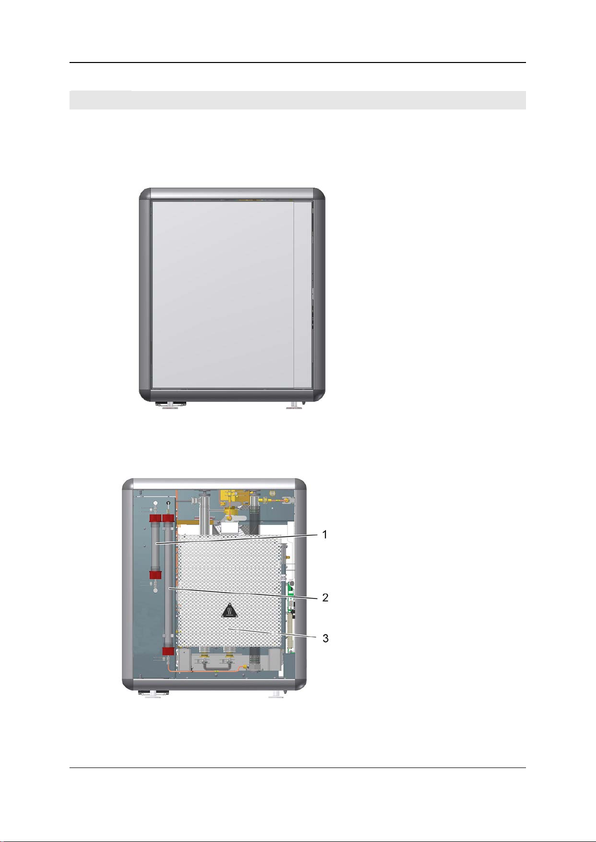
3 - Product description 36
Front view
Front view, closed
The following picture shows the front view of the instrument with the front door closed:
Front view, open
The following picture shows the front view of the instrument with the front door opened:
Legend:
1 Ball valve
2 Drying tubes
3 Furnace with heat protection cladding
Operating instructions DuMaster D-480 ©BÜCHI Labortechnik AG
Page 37

3 - Product description 37
Rear view
Rear view
The following picture shows the rear view of the analyzer:
Legend:
1 Rear wall
2 Air baffle
3 "PC" PC connector (USB)
4 "Reserve" reserve
5 "~" mains connector
IN" CO2 gas inlet
6 "CO
2
7 "O2 IN" O2 gas inlet
8 Gas drying
9 "WASTE" Gas outlet
Right side view
Right side view, closed
The following picture shows the right side of the analyzer with the side door closed, as seen from the
front:
Legend:
1 Right side door
2 Main switch
Operating instructions DuMaster D-480 ©BÜCHI Labortechnik AG
Page 38

3 - Product description 38
Right side view, open
The following picture shows the right side of the analyzer with the side door open, as seen from the
front:
Legend:
1 Mainboard
2 Furnace
3 Main switch
Left side view
Left side view, closed
The following picture shows the left side of the analyzer with the side door closed, as seen from the
front:
Legend:
1 Left side door
Operating instructions DuMaster D-480 ©BÜCHI Labortechnik AG
Page 39
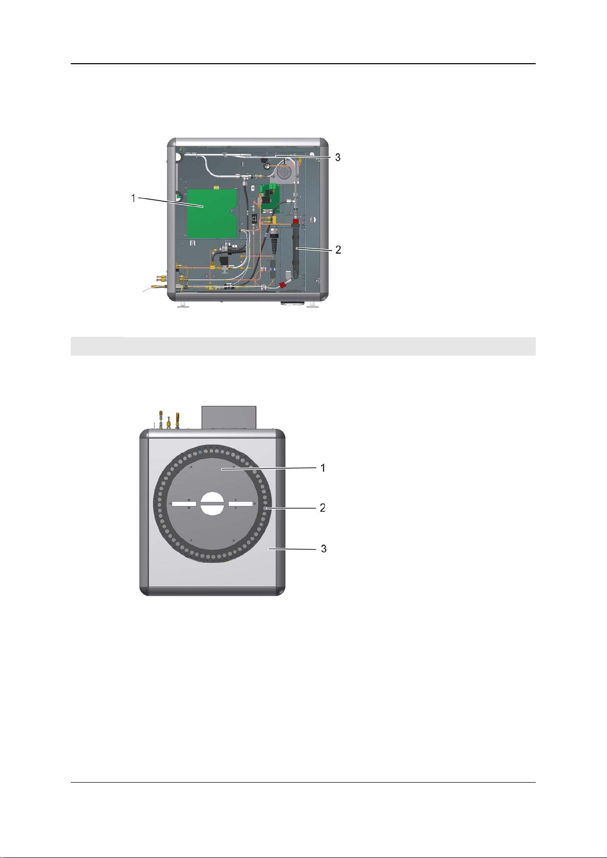
3 - Product description 39
Left side view, open
The following picture shows the left side of the analyzer with the side door open, as seen from the
front:
Legend:
1 Thermal conductivity detector (TCD)
2 Water condenser
3 Gas drying
T op view
Top view of the instrument
The following picture shows the top view of the instrument:
Legend:
1 Carousel cover
2 Carousel, sample magazine and
cover ring
3 Instrument cover
Operating instructions DuMaster D-480 ©BÜCHI Labortechnik AG
Page 40

3 - Product description 40
Peripherals and t heir funct ion
Peripheral
Function
Requirement
Types of peripherals
The following picture shows the analyzer and its peripherals
Functions of the peripherals
The following table lists the functions of peripherals:
PC Operation of the instrument with operating software required
Printer Print out measuring results, etc. recommended
Balance Transmit sample weight recommended
Legend:
1 Instrument
2 Balance
3 Printer
4 PC
Operating instructions DuMaster D-480 ©BÜCHI Labortechnik AG
Page 41

Data administration and data security ...........................................................................................69
CHAPTER 4
Understanding the i ns t r um ent a nd planning
its use
Target group
Personnel with basic chemical knowledge and basic computer knowledge.
Purpose
This section helps you to assess the applications of the instrument and subsequently plan the use of
the instrument.
In this chapter
Layout and mode of functioning ....................................................................................................42
Processes in the instrument during a measurement......................................................................46
Basic facts about working with the instrument ...............................................................................49
Understanding the operating software ...........................................................................................58
Operating instructions DuMaster D-480 ©BÜCHI Labortechnik AG
Page 42

4 - Understanding the instrument and planning its use 42
Layout and mode of functioning
The thermal conductivity detector (TCD) .......................................................................................45
Target group
Personnel with basic chemical knowledge and basic computer knowledge.
Purpose
This section describes what the instrument does, what the analysis parameters mean, and what
happens in the instrument during an analysis.
In this section
Functional units .............................................................................................................................43
Operating instructions DuMaster D-480 ©BÜCHI Labortechnik AG
Page 43

4 - Understanding the instrument and planning its use 43
Functional units
Introduction
The following section describes what units comprise the instrument and what functions the individual
units perform in the analysis procedure.
Functional diagram
The following diagram shows the basic setup of the instrument and its division into functional units.
Operating instructions DuMaster D-480 ©BÜCHI Labortechnik AG
Page 44

4 - Understanding the instrument and planning its use 44
I Mechanical sample insertion and O2 dosing system
Part
Name
Function
Part
Name
Function
Part
Name
Function
II Furnace area and reaction zone
III Gas drying
IV Detector
Mechanical sample insertion and O2 dosing system (I)
The following table describes the components of the unit and their functions:
1 Carousel
2 Ball valve with Ni flap
For details on sample insertion, cf. Sample insertion and initiation of measurement (on page 47).
Furnace area and reaction zone (II)
The following table describes the components of the unit and their functions:
3 Furnace
4 Combustion tube with tube
filling
5 Ash crucible
6 Post combustion tube with
tube filling
7 Reductor
holds all samples in a series.
transports the current sample into the ball valve
allows the metered addition of O2 during the combustion.
holds the current sample.
shuts the current sample off from the ambient air.
allows the system to displace any ambient air.
transports the current sample into the combustion tube.
protects the ball valve from contamination.
holds the combustion tube, post combustion tube and
reductor/regainer at a constant temperature and thereby
ensures reproducible analysis results.
Space for complete combustion of the sample including
combustion catalyst.
Binds disturbing alkali and earth alkali elements.
Holds combustion residues and sample packing of
analyzed samples; for fast, easy emptying without
replacing the combustion tube.
Oxidation of the combustion products.
Reduces NOX to N2.
Binds volatile halogen compounds and sulfurous
compounds.
For details on the processes in the furnace area, cf. Substance digestion and preparation of the
reaction gas mixture.
Gas drying (III)
The following table describes the components of the unit and their functions:
8 Drying tube, gas drying and
water condenser
Operating instructions DuMaster D-480 ©BÜCHI Labortechnik AG
Removes H2O from the measuring gas.
Page 45

4 - Understanding the instrument and planning its use 45
Detector (IV)
Part
Name
Function
The following table describes the components of the unit and their functions:
9 Reference cell
10 Measuring cell
For details on the working principle of the detectors, see Detecting measuring components and
evaluating the measuring signal (on page 48).
reacts to fluctuations in the composition of the analysis gas
mixture with an electrical signal to which a measuring
component can be assigned.
see "Reference cell".
The thermal conduct ivity det ector (TCD)
Design
The thermal conductivity detector (TCD) consists of two chambers through which the analysis gas
mixture (measuring cell) and the pure carriage gas (reference cell) simultaneously flow through during
the analysis. The chambers form a measuring bridge.
Working principle
The thermal conductivity of the carrier gas reacts sensitively on the addition of small amounts of
foreign gases such as the measuring component N. If this measuring component exists in the
analysis gas mixture, this leads to a disturbance of the measuring bridge that is registered in the form
of an electrical signal.
Further processing of the measuring signal
The TCD measuring signal is digitized, integrated and output by the instrument to the PC, where it is
registered in the form of a measuring peak dependent on time,
and the integral is correlated with the absolute quantity of the respective measuring component
by calibration functions.
Operating instructions DuMaster D-480 ©BÜCHI Labortechnik AG
Page 46

4 - Understanding the instrument and planning its use 46
Processes in the instrument during a measurement
Formulas for determining element concentration of analysis samples (Solids) .............................48
Target group
Personnel with basic chemical knowledge and basic computer knowledge.
Purpose
The following section is designed to help you understand the processes that take place during a
measurement.
In this section
Sample insertion and initiation of measurement ............................................................................47
Substance digestion and preparation of the reaction gas mixture .................................................47
Detection of measuring components and evaluation of the measuring signal ...............................48
Operating instructions DuMaster D-480 ©BÜCHI Labortechnik AG
Page 47

4 - Understanding the instrument and planning its use 47
Sample inserti on and initi ation of measure ment
Introduction
The following section explains how to insert the analysis samples into the combustion tube and how
to initiate measurement of the reaction products.
Note
The bracketed numbers used below refer to the part numbers listed in Functional units.
Sample insertion processes and initiation of measurement
Sample insertion and initiation of measurement is divided into the following phases:
The thermal conductivity detector (9, 10) performs autozero adjustment of the measuring signal.
A complete pressure drop takes place in the system, together with the emptying of water
accumulated in the water condenser (8).
The ball valve (2) opens by turning the ball through 90°.
The carousel (1) moves one step and the sample drops through the ball valve (2) onto the closed
Ni flap.
The ball valve (2) turns through 90° and closes the apparatus.
The carrier gas is reactivated and and the atmospheric nitrogen will be flushed out.
After expiration of a flushing time (Ni flap delay) the Ni flap opens for a short period by means of
a pivoting magnetic field.
The sample drops into the ash crucible (5) of the combustion tube (4) and is heated up to the
combustion temperature.
Oxygen dosing into the ash crucible begins.
The integrator reset resets integration display to zero. N integration begins.
Substance digesti on and pre paration of th e reaction g as mixtur e
Introduction
The following section explains
what processes take place in the combustion, post combustion and reductor of the furnace.
how the reaction gas mixture is prepared for the nitrogen determination.
Note
The item numbers used below refer to the picture in Functional units.
Processes during substance digestion and preparation of the reaction gas mixture
Substance digestion and preparation of the reaction gas mixture is divided into the following phases:
The atmosphere in the combustion tube (4) is enriched with oxygen. Nitrogen bound in the
sample burns to form N
compounds, sulfur reacts to form SO2 and SO3, hydrogen reacts to form H2O and carbon reacts
to form CO
The carrier gas flow transfers the gaseous combustion products into the post combustion tube (6)
and reductor (7), where the following processes take place:
In the reductor, nitrogen oxides are quantitatively transferred to form molecular nitrogen.
Sulfur absorption takes place in the reductor.
Volatile halogen compounds are bound on brass wool.
.
2
and NOX. Halogens bound in the sample react to form volatile halogen
2
Operating instructions DuMaster D-480 ©BÜCHI Labortechnik AG
Page 48

4 - Understanding the instrument and planning its use 48
The post combustion tube is used to complete oxidation of the sample.
The gas stream is predried in the water condenser (8) as well as the gas drying. In the
downstream gas drying and drying tube (8), the residual moisture is removed.
Detection of measur ing compon ents and evalu ation of the m easuring sig nal
Introduction
The following section explains how the measuring components are detected in the reaction gas
mixture and how the measuring signal is evaluated.
Process
Detection of the measuring components and evaluation of the measuring signal take place in the
following phases:
Depending on the type and concentration of the measuring component, the thermal conductivity
detector sends an electrical measuring signal to a microcontroller. This controller integrates the
measuring signal. Cf. The thermal conductivity detector (TCD) (on page 45).
In the PC the measuring signal
is recorded dependent on time
and displayed as an integral.
The integral value is assigned to an absolute nitrogen content of the sample via a non-linear
calibration. See Background knowledge required for calibration (on page 51).
The nitrogen percentage of the sample is calculated from the found absolute nitrogen content
and the sample weight. An empirical factor (protein factor) translates the nitrogen content to the
protein content.
Formulas for determ ining eleme nt concent ration of analysis s amples (S olids)
Process
During an analysis, the system first measures the absolute element content of the sample.
The peak area value of the N component of the sample is determined.
The blank value is factored in.
The absolute N content of the sample is computed on the basis of the calibration coefficients.
The daily factor is factored in.
The N concentration of the sample is calculated from the computed absolute N content and the
sample weight by the following formula:
where:
c = element concentration in [%]
a = absolute element content in [mg]
f = daily factor
w = sample weight in [mg]
Operating instructions DuMaster D-480 ©BÜCHI Labortechnik AG
Page 49

4 - Understanding the instrument and planning its use 49
Basic facts about working with the instrument
Formula for determining the daily factor ........................................................................................57
Target group
Personnel with basic chemical knowledge and basic computer knowledge.
Purpose
The following section provides basic facts about working rationally and appropriately with the
instrument.
In this section
Instrument equipment ....................................................................................................................50
Background knowledge required for calibration .............................................................................51
Calibration curve calculation method criteria .................................................................................52
Calibration formulae ......................................................................................................................54
Routine measuring work ................................................................................................................55
Formulae for blank value determination and compensation ..........................................................56
Operating instructions DuMaster D-480 ©BÜCHI Labortechnik AG
Page 50

4 - Understanding the instrument and planning its use 50
Instrument equi pment
Combustion tube filling
The following picture shows the fillings and filling heights of the combustion tube:
Legend:
1 Ash crucible
2 Corundum balls (10 mm)
3 80 g CuO + 20 g Corundum balls (87 mm)
4 Corundum balls (26 mm)
5 Wire mesh ronde
6 Spacer
Filling the post combustion tube
The following picture shows the fillings and filling heights of the post combustion tube:
Legend:
1 Plug with embedded 3.3g brass wool
2 53g Regainer (126 mm)
3 Quartz wool (10 mm)
4,180 g CuO + 15 g Pt catalyst (167 mm)
5 Corundum balls (28 mm)
6 Wire mesh ronde
7 Spacer
Operating instructions DuMaster D-480 ©BÜCHI Labortechnik AG
Page 51

4 - Understanding the instrument and planning its use 51
Background knowle dge requir ed for calibr ation
Important calibration principles
Perfect calibration of the instrument is a key condition for achieving correct analysis results. The
calibration has to be carried out over the whole measuring range.
For successful calibration the user must be familiar with the analyzer and the operating instructions.
The personnel performing calibration must therefore be authorized and must have undergone
appropriate training.
Purpose of instrument calibration
The analyzer does not measure the absolute content of an element in the sample but rather only
changes of the element portion in the combustion gases. These changes cause an electrical signal in
the detector that is recorded and integrated by the software depedent on time.
In order to create a correlation between the integrated detector signal and the absolute element
content of the analysis samples, a series of calibration samples with known element content and
different sample weights are measured. The software computes the calibration factors on the basis of
the known element contents and the sample weights of the calibration samples.
Conditions for perfect calibration
In order to be able to calibrate the instrument perfectly, the following conditions must be met:
The instrument must have passed the leak test.
The instrument blank values must be low and roughly constant.
Only use suitable substances of at least p.a. quality or certified standards as calibration samples.
The concentration values of the calibration samples must cover the whole measuring range.
When to calibrate the instrument
It is always necessary to calibrate the instrument when one of the following is true:
You have removed components that influence analysis results, e.g. the detector.
The daily factor for a measuring component is clearly outside of the range of 0.9 to 1.1. Also, it
displays fast changes in time from day to day.
Calibration formulae
The formulae used for calibration can be found in Calibration formulae (on page 54).
Calibration curve calculation method
For details on the various calibration curve calculation methods and when to use them, see
Calibration curve computati on meth od criter i a (on page 52).
Notes on performing calibration
For details on practical implementation of calibration, refer to
the section Performing calibration.
the calibration tables.
Operating instructions DuMaster D-480 ©BÜCHI Labortechnik AG
Page 52

4 - Understanding the instrument and planning its use 52
Calibration curv e calculati on method cri teria
Calibration curve configuration options
The user can specify the calibration curve calculation method according to the following criteria:
Calibration can be performed over the whole measuring range either consistently or in two
ranges.
For a specific element content you can set a dividing line for two calibration ranges.
For each range, you select a polynomial degree according to which to compute the calibration
curve (linear to 4th degree).
Calculation criteria
Look to the calibration view of the combi view for calibration curve calculation method criteria. You get
to the calibration view after performing or loading a series of defined calibration samples by selecting
Calibration > Calibrate... and then the "Configuration calibration" dialog.
Ideal calculation method
If possible, try to compute calibration curves so that they
are uniform over the whole measuring range and/or concentration range
and can be displayed in linear form or on the basis of a polynomial of the lowest order.
To facilitate selecting a calculation method, four typical calibration graphs are shown below along with
the suitable calculation method.
Note: For better understanding the calibration graphics are shown in a simplyfied way.
Linear calculation over the whole range
The following picture shows an example in which a linear calculation over the whole range achieves
acceptable calibration curve quality.
Operating instructions DuMaster D-480 ©BÜCHI Labortechnik AG
Page 53

4 - Understanding the instrument and planning its use 53
Linear calculation over two ranges
The following picture shows an example in which a linear calculation over two ranges achieves
acceptable calibration curve quality.
Linear and polynomial calculation
The following picture shows an example in which the calibration curve exhibits acceptable quality by
means of a linear calculation in the low concentration range and a polynomial calculation in the higher
concentration range.
Polynomial calculation over the whole range
The following picture shows an example in which a polynomial calculation over the whole range
achieves acceptable calibration curve quality.
Achievable calibration curve quality
Process standard deviation "Proc-SD" and quality factor "r" serve as a measure of achievable
calibration curve quality.
Operating instructions DuMaster D-480 ©BÜCHI Labortechnik AG
Page 54

4 - Understanding the instrument and planning its use 54
Use the following values for process standard deviation "Proc-SD" as guidelines:
Acceptable value: Proc-SD = ±3 µg in the lower range
Proc-SD = ±15 µg in the upper range
Very good value: Proc-SD = ±1 µg
Use the following values for quality factor "r" as guidelines:
Good value for linear calibration function: r = 0.99 (r should tend to 1)
Good value for polynomial as calibration function r = < 2-4 (r should tend to 0)
If you do not approximately achieve the listed values you can assume that you have chosen the
wrong calibration curve calculation method.
Calibration for mulae
Calculation of absolute element content
Calibration is performed by analyzing samples with known concentrations (standard samples) where
the measured peak areas are correlated with the corresponding absolute element content.
For a standard sample, the following parameters are known:
element concentration
Weight
Absolute element content is computed according to this formula:
Computing calibration coefficients
Once the absolute element contents have been computed and the peak areas have been measured
for the respective sample, the pairs of values (absolute content / peak area) are transferred into a
coordinate system where they form the calibration curve. By means of an algorithm, the calibration
coefficients a - e are computed which, entered in a polynomial, constitute the calibration curve.
Absolute element content is computed according to this formula:
where:
a = absolute element content in [mg]
w = sample weight in [mg]
c = element concentration in [%]
where:
y = absolute element content in [mg]
a...e = calibration coefficients
x = peak area
Computing the quality factor for polynomials of the 1st degree
In order to assess how well the calibration curve described by the polynomial follows the actual
development of the pairs of values, the software computes a quality factor for each calibration
process. For a polynomial of the 1st degree (linear equation), this quality factor corresponds to the
correlation coefficient. The closer the correlation coefficient tends to 1, the better the fit.
Operating instructions DuMaster D-480 ©BÜCHI Labortechnik AG
Page 55
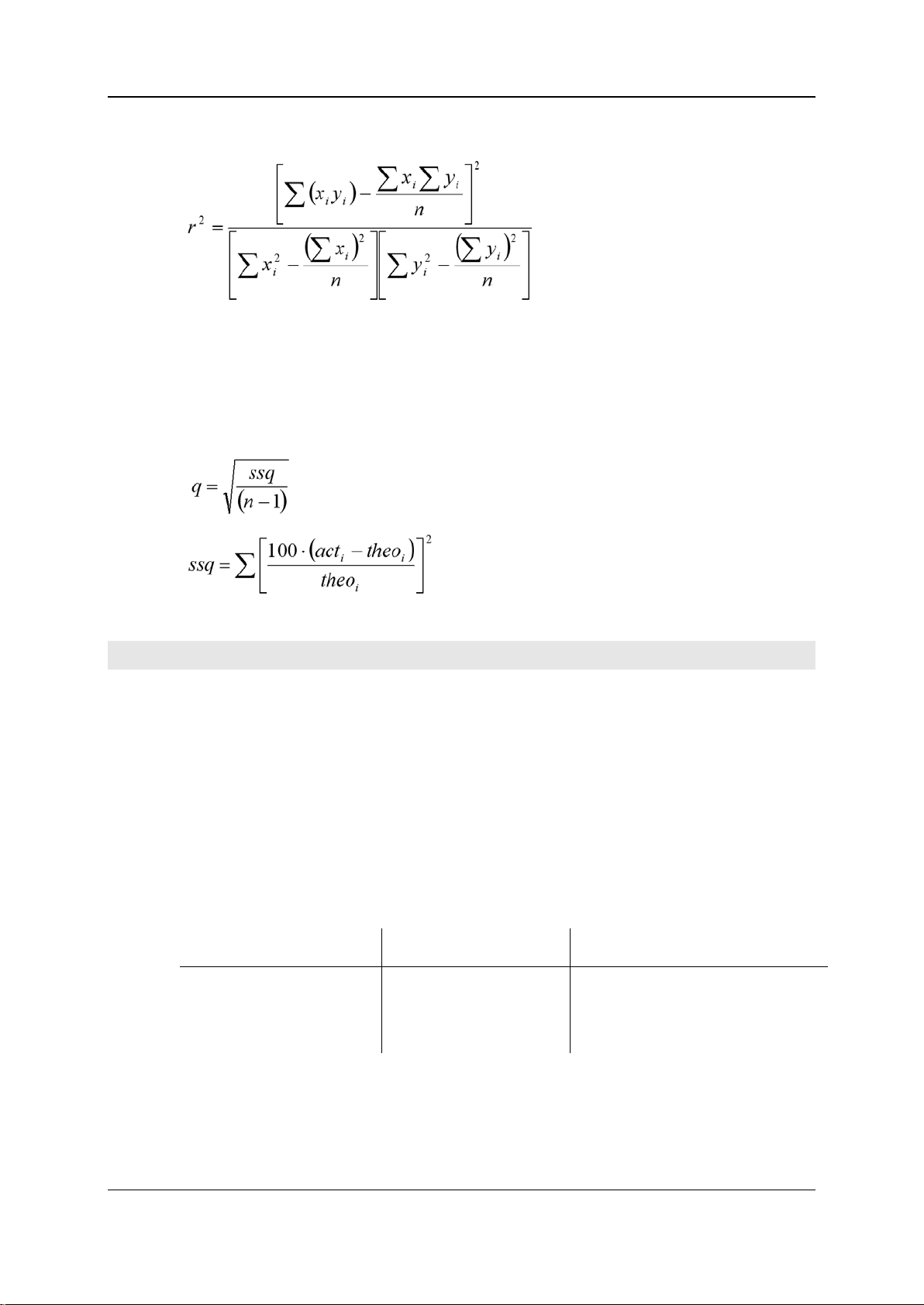
4 - Understanding the instrument and planning its use 55
The correlation coefficient is computed according to this formula:
Computing the quality factor for polynomials of a higher degree
In order to assess how well the calibration curve described by the polynomial follows the actual
development of the pairs of values, the software computes a quality factor for each calibration
process. For a polynomial of a higher degree, this quality factor corresponds to the sum of the error
squares. The closer the sum of error squares tends to 0, the better the fit.
The sum of error squares is computed with these formulae:
where:
q = quality
ssq = sum of error squares
= actual absolute content computed respectively
act
i
= theoretical absolute content respectively
theo
i
n = number of samples
i = index from 1 to n
where:
r2 = correlation coefficient
xi = peak area of the corresponding sample
= absolute content of the corresponding
y
i
sample
n = number of samples
i = index from 1 to n
Routine measurin g work
Definitions
Routine measuring work comprises the following activities:
Determination of instrument blank values.
Instrument conditioning with conditioning samples.
Determination of daily factors.
Routine measuring work is performed at set intervals or on defined occasions before, during or after a
series of measurements with real samples.
Instrument blank values
Determination of the instrument blank value depends on your needs. The following overview shows
the type and purpose of the individual determinations.
Purpose Sample Occasion
Checking gas-tightness none after maintenance work
Blank value determination of
sample additives and packing
materials
Sample additive
Packing material
to allow for sample additives or packing
material
For details on determining blank values, cf. Types of blank value determination and their settings.
Operating instructions DuMaster D-480 ©BÜCHI Labortechnik AG
Page 56

4 - Understanding the instrument and planning its use 56
Conditioning samples
Conditioning samples are measured with standard substances at the start of every series of analyses.
They are used to check...
... the correct run of the analysis.
... the proper condition of the instrument.
... flow and pressure behavior of the gases.
Daily factor determinations
Determination of the daily factor serves...
... to fine-tune instrument calibration to room conditions at the time of analysis.
... to assess the condition of the instrument by observing daily factor fluctuations and drift trends.
When to perform routine measuring work
Perform routine measuring work...
... at least once a day.
... additionally when measuring breaks last longer than 2 hours.
If a series of analyses exceeds a duration of 5-6 hours (carousel completely loaded), it is advisable to
determine the daily factor additionally at the end of the series.
Formulae for blan k value determ ination a nd compensati on
Blank samples and blank values
Blank samples are samples...
... that do not contain sample substance.
... that have a key word for identification by the software as blind samples.
Despite the lack of sample substance, a peak area value is computed on the basis of various factors
when analyzing blank samples. This peak area value is referred to as a blank value. In order to
compensate for this, the averaged blank value is subtracted from the measured peak area value of
every individual analysis sample.
Blank value determination
In blank value determination, the peak area values of the blank samples are averaged. The blank
value is computed according to this formula:
Blank value compensation
where:
/b = blank value
= peak areas of the individual blank samples
b
i
n = number of blank samples
i = index from 1 to n
The peak areas of the other samples are compensated with the aid of this formula:
where:
a
= compensated peak area
comp
a = measured peak area of the sample
/b = blank value
Operating instructions DuMaster D-480 ©BÜCHI Labortechnik AG
Page 57

4 - Understanding the instrument and planning its use 57
Formula for determ ining the dai ly factor
Determining the daily factor
Standard samples are analyzed to determine the daily factor. The known element concentration of the
standard samples is correlated with the actual element concentration computed.
Daily factor
The daily factor is computed according to this formula:
whereas:
f = daily factor
c
c
= theoretical element concentration
theo
= element concentration computed actually
act
Operating instructions DuMaster D-480 ©BÜCHI Labortechnik AG
Page 58

4 - Understanding the instrument and planning its use 58
Understanding the operating software
Right mouse button function ..........................................................................................................67
Target group
Personnel with basic chemical knowledge and basic computer knowledge.
Purpose
This section describes
the layout of the user interface
what instrument functions are controlled by the software
what current information is displayed during the analysis process
and how the raw analysis data are further processed, archived and managed
In this section
Basic functions of the operating software ......................................................................................59
Software user interface ..................................................................................................................60
Sample view ..................................................................................................................................61
Combi view ....................................................................................................................................63
Status view ....................................................................................................................................66
Operating instructions DuMaster D-480 ©BÜCHI Labortechnik AG
Page 59

4 - Understanding the instrument and planning its use 59
Basic functions of the operating software
Introduction
The following section describes the functions of the operating software and what instrument control
and data processing operations are possible.
Instrument control and parametrization
Instrument control and parametrization functions:
Starting a single analysis:
Starting and stopping a series of analyses
Entering parameters to prepare the instrument for measuring and for standby mode transitioning
(wake-up and sleep functions)
Determination of methods
Specifying time and temperature parameters of the analyzer
Data input
Data input functions:
Injection volume (via method)
Sample weight (solids mode)
Name
Blank values
Processing measuring data
Measuring data processing functions:
Measurement and numerical output of element contents in absolute values and percentages
Statistical evaluation of analysis data
Management of analysis data; data security
Analysis data management and data security functions
Importing/exporting from and to MS Excel
Interfaces to LIMS
Security functions using digital signatures
Support for maintenance/repair
Maintenance and repair support functions:
Definition of maintenance events and display when due
Calculation of calibration coefficients and assessment criteria for calibration quality
System diagnostics functions
Display analysis values and instrument state
Functions for current analysis value and current instrument state display:
Analysis progress
Temperature of the reaction tubes
Gas flows and pressure conditions in the instrument
Due time/date of next maintenance event
Current detector display
Element content of current sample
Operating instructions DuMaster D-480 ©BÜCHI Labortechnik AG
Page 60
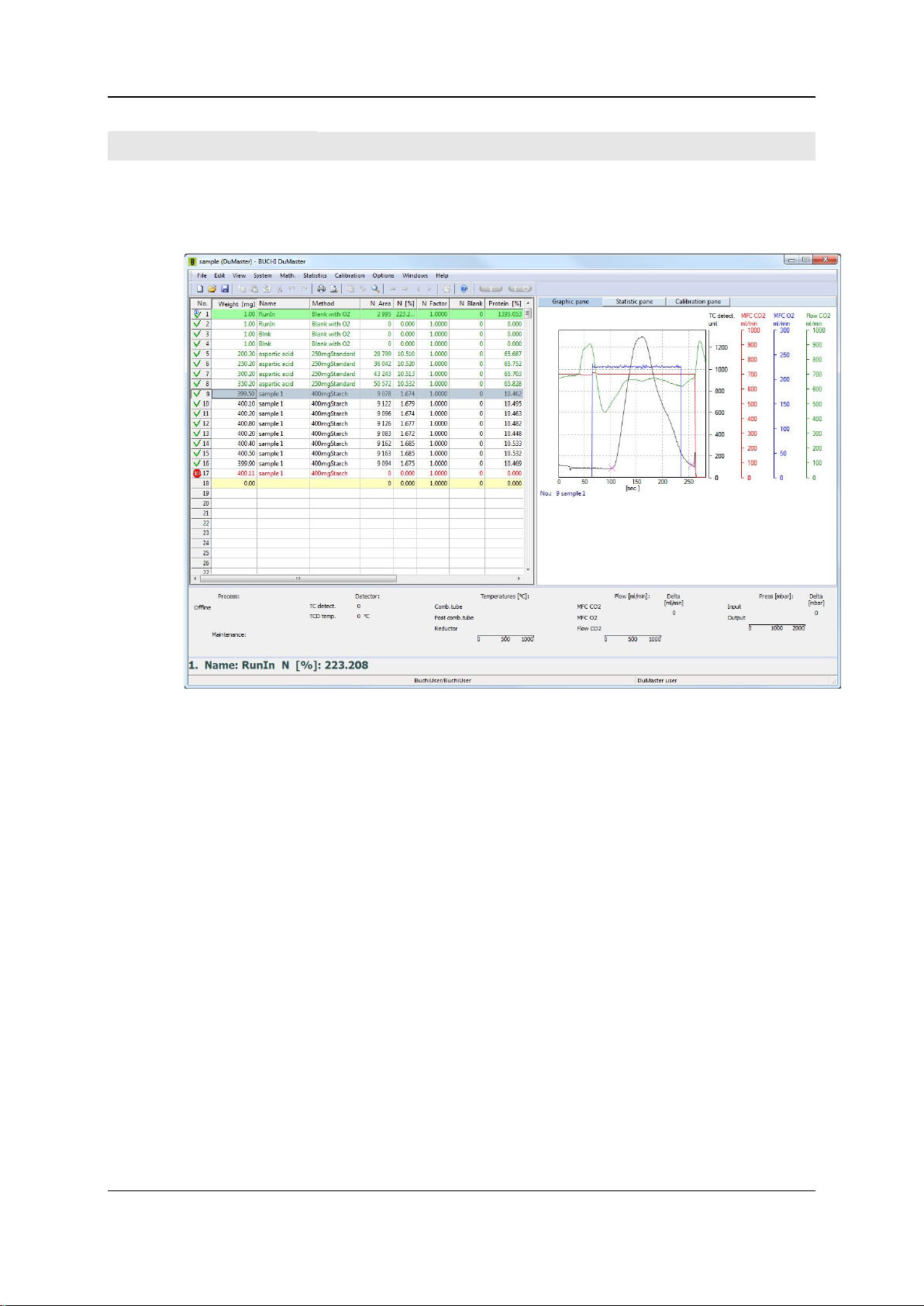
4 - Understanding the instrument and planning its use 60
Software user inter face
The main window of the operating software
The following screenshot shows the main window of the operating software and designates the
various areas and bars:
Title bar
Menu bar
Toolbar
The title bar displays the name of the file that you are currently processing. The title bar has the usual
functions for displaying the system menu and for minimizing, maximizing and closing the window.
The menu bar shows the top level of the menu tree. You can access dialogs and input windows, etc.
from the menubar for the following:
Saving, editing and managing analysis data,
Defining and entering sample data and instrument parameters,
Specifying maintenance events,
Configuring and performing statistical evaluations.
Details on the various dialogs and input windows accessible from the menu bar can be found at Menu
and dialog descriptions (on page 251) and in the online help.
The toolbar allows you quick access to frequently required commands and functions. Among others,
via the toolbar you can...
... create or save analysis series in the form of a file and open existing analysis files.
... cut, copy and paste sample data.
... switch the sample view.
... enable statistical and calibration functions.
Operating instructions DuMaster D-480 ©BÜCHI Labortechnik AG
Page 61

4 - Understanding the instrument and planning its use 61
... "wake up" the "sleeping" instrument.
... start and stop individual and continuous analyses.
... display the online help.
Details on the various buttons on the toolbar can be found at Toolbar (on page 333) and in the online
help.
Sample view
The sample view displays a table of input, measuring and computed analysis data of all samples in a
particular series. If an error occurs while measuring a sample, the table contains an appropriate
message. For details on the sample view, see The sample view.
Combi view
The combi view contains different information depending on the selected display mode:
In progression/graph view, it displays the time-dependent development of the detector signals or
a diagram of various instrument parameters of the currently selected sample.
In statistics view it displays statistical analysis data of the selected group of samples.
In calibration window view it displays a diagram of the calibration factors for the series under
review and the calibration curves of the individual elements.
For details on the combi view and its various display modes, see The combi view.
"Current sample" field
This field displays a zoomed-in view of the data of the current sample. Here you can view the analysis
results of the particular sample at a glance, even if you are not directly in front of the screen.
Status view
The status view contains information about the current operating states of the elemental analyzer. For
details on the status view, See The status view.
Status bar
The status bar can contain the following information:
If you hover the mouse over a menu command or toolbar button, a short help text on the
command is displayed on the left of the status bar.
The name of the current user logged in is displayed in the middle of the status bar.
The name of the user group to which the currently logged in user belongs is displayed on the
right.
Sample view
Introduction
The following section describes what you can input in the sample view and what information you can
get from the sample view.
Operating instructions DuMaster D-480 ©BÜCHI Labortechnik AG
Page 62

4 - Understanding the instrument and planning its use 62
View
Column
Explanation
Color code
Meaning
The sample view looks like a familiar calculation sheet in a spreadsheet program.
Sample view input functions
In the sample view you define the sequence of your analysis samples. The sequence must match the
sequence in which you arrange your samples on the carousel. To enable the instrument to analyze
and evaluate a sample correctly, you must have entered the appropriate information in the sample
view columns:
Weight [mg] Sample weight in mg (if the instrument is not connected to a balance that
Name Name of the sample; for samples used for routine measuring work you must
Method Assignment of an analysis method. If you have entered values for peak
In the "Memo" column you can input any special features of the sample or the analysis procedure as
free text.
Color coding
Some table lines in the sample view are highlighted by a colored background or colored text. The
following table indicates the meaning of the various color codes:
green background Indicates the current sample.
yellow background Indicates the current sample.
red text Indicates a sample with a stop marker set.
green text Indicates samples with reserved names for routine measuring work or
black text Indicates all other samples.
automatically transfers the sample weight to the computer).
use the reserved names, see Defining standard substances as factor and
monitor samples (on page 120) and Defining standard substances as
calibration samples (on page 120).
anticipation in the "Method" dialog, this overwrites the values for individual
samples that were defined in the "Device parameters" dialog for the series.
calibration samples.
Operating instructions DuMaster D-480 ©BÜCHI Labortechnik AG
Page 63

4 - Understanding the instrument and planning its use 63
Meaning of symbols in the "No." column
Icon
Meaning
In the "No." column a symbol is displayed next to the serial number generated by the system; this
symbol indicates the status of the individual samples. The following table lists the possible symbols
and what they mean.
Sample not yet analyzed, but a measuring method has been set and a sample name
exists.
Sample not yet analyzed, but a sample name has been set and a method does not yet
exist.
Sample analyzed error-free with valid date information.
Sample without valid date information.
Sample which caused a non-critical error during measurement or when the measured
peak area is outside of the specified calibration. The result was interpolated. The error
code is entered in the "Info" column, see Interpreting PC error messages (on page
238).
Sample at which the series was stopped.
Further information in the sample view
Depending on the selected operating mode, the following values can be displayed in the appropriate
columns for each analyzed sample:
the integrals of the samples
the element content percentages of the samples
the daily factors of the elements for the particular sample
the blank values of the elements for the particular sample
date and time of measuring the particular sample
By selecting the View > Configuration menu you can show/hide every table column and define the
order as desired.
Note on data output
The selected sample view screen view also corresponds to the display in a printed report.
Combi view
Introduction
The following section describes the various views of the combi view and their information contents. By
selecting the View > Toggle menu you can switch between the following combi views:
Progression view (graph view)
Statistics view
Calibration view
Operating instructions DuMaster D-480 ©BÜCHI Labortechnik AG
Page 64

4 - Understanding the instrument and planning its use 64
Progression view (graph view)
Progression view displays a graph of the development over time of important instrument parameters
and measured values during measurement of the sample selected in the sample view. You can
recognize the current sample by the green border around the graph display.
You can display the following individual parameters and measured values:
The CO2 gas flow through the MFC
The O
The CO2 gas flow through the flow meter
The intake pressure
The output pressure
The detector output signal
For details on configuring the analysis progression view, see Data backup and printing (on page
156).
Statistics view
gas flow through the MFC
2
Operating instructions DuMaster D-480 ©BÜCHI Labortechnik AG
Page 65

4 - Understanding the instrument and planning its use 65
The statistics view displays the element content percentages of all samples in a series, grouped by
sample name.
For each group of samples, the following calculated statistical values per element are also displayed:
Percentage mean value of the element
The absolute standard deviation of the mean values
The relative standard deviation of the mean values
Difference (Delta) of the highest and lowest content of the group
You can exclude individual samples and/or values of a group from the calculation of statistical values
or include them again.
Calibration view
If your series includes samples previously defined as calibration samples, you can use them to
calculate calibration coefficients. You can define and determine up to two calibration ranges
according to which polynomial degree you want to determine the calibration curve.
In this case, the calibration view displays the following information:
For each defined calibration range a graph display of the calibration curve optimized for the
respective calibration samples.
The calibration coefficients computed according to the selected polynomial degree.
The correlation coefficient for the depicted calibration curve that allows you to assess the quality
of calibration.
Operating instructions DuMaster D-480 ©BÜCHI Labortechnik AG
Page 66
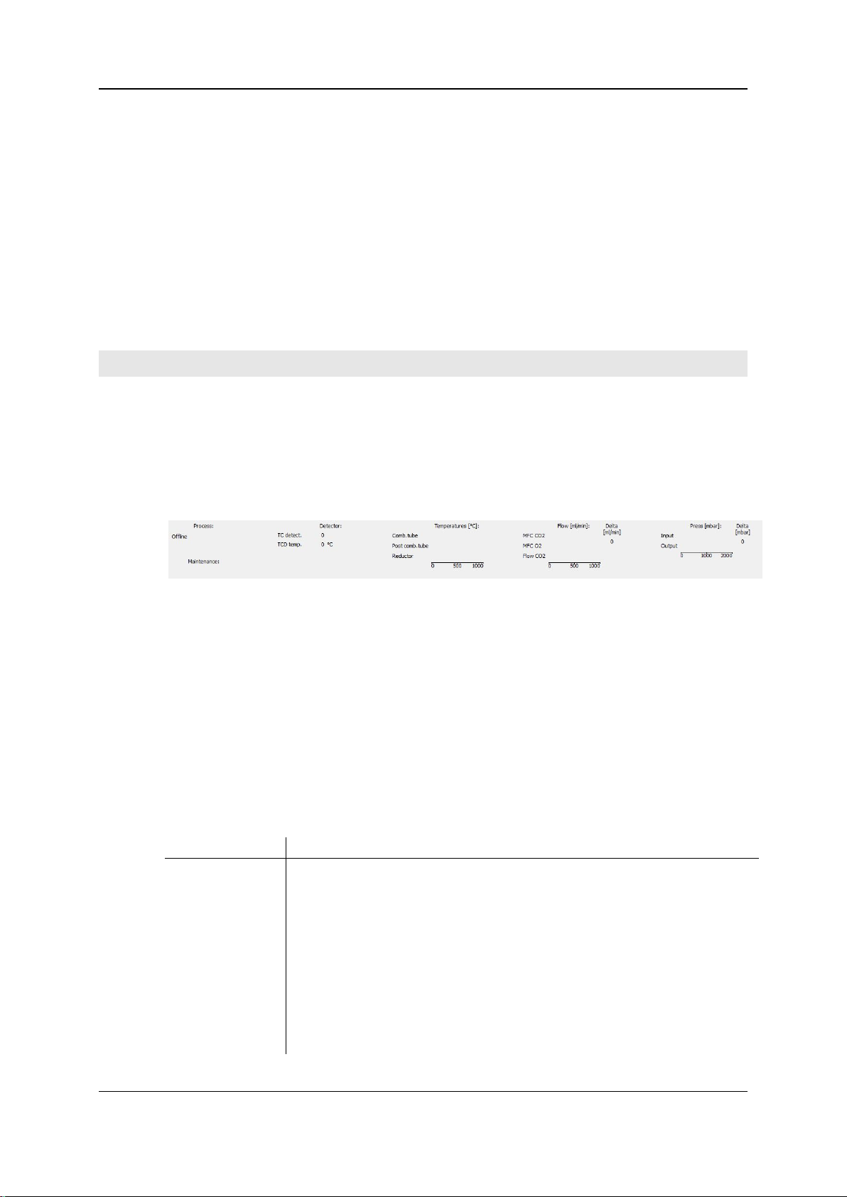
4 - Understanding the instrument and planning its use 66
In the graph display, the samples used for compute the calibration curves are displayed as small
Area
Meaning
circles. You can click one of these circles to display further information on the particular sample, see
Background knowledge required for calibration (on page 51). This information allows you to
assess whether the sample must be treated as an "outlier" and therefore excluded from the
calculation of the calibration coefficients. If you have assessed the calibration curves in this way and
browse on to the next view, the "calibration coefficient" dialog is displayed with the current computed
values. When you confirm this dialog by clicking OK, the calibration coefficients for the series are
applied and the content of the calibration view is deleted (message: "No calibration or calibration
finished").
Note on data output
The selected screen view of the combi view also corresponds to the display in a printed report.
Status view
Introduction
The following section describes what information about the analysis procedure and the condition of
the instrument is displayed in the status view.
View
The following screenshot shows the status view in offline status:
Meaning of the colored background
On the basis of the color of the status view background you can tell straight away whether the PC is
properly connected to the analyzer. The meaning of the colors is:
green: The analyzer is connected to the PC and switched on. With the aid of the PC you can
enter analysis or instrument parameters
start or abort analyses
perform maintenance or diagnostics tasks.
gray: The analyzer is not connected to the PC or switched off. The operating software is running
in offline status.
The areas of the status view and what they mean
The following table lists the individual areas of the status view and the information they contain:
Process Displays a list of individual processes during the analysis procedure. The current
process is highlighted with a colored background so that you can see the
progress of the analysis of the current sample straight away. Displays "Standby"
when the instrument is in idle mode.
Detector Displays the following current values of the detector unit:
the current height of the current measuring peak.
Temperatures Displays the current temperatures of the following units as a bar chart:
Combustion tube
Post combustion tube
Reductor
Operating instructions DuMaster D-480 ©BÜCHI Labortechnik AG
Page 67

4 - Understanding the instrument and planning its use 67
Flow The current gas flow is displayed here as a bar chart.
When a maintenance interval is due, its name is displayed as text on the bar chart
Command
Meaning
Command
Meaning
MFC CO2: CO
MFC O2: O
Flow CO2: CO2 flow through the analysis apparatus
In addition to bar graph the numerical value of the gas flow is displayed.
Position the cursor on the corresponding end of a bar graph.
Pressure Displays the current pressure values in the instrument here as bar diagram:
Input: Pressure value at the entrance section
Output: Pressure value at the exit section
In addition to bar graph the numerical value of the pressure is displayed.
Position the cursor on the corresponding end of a bar graph.
Maintenance Maintenance intervals for the analyzer are defined on the basis of the maximum
number of measured samples until a certain maintenance event occurs, see
Defining maintenance intervals in the software. The "Maintenance" section
displays the current percentage of the specified number of samples until the next
maintenance interval. This figure is displayed numerically and as a bar chart. The
colors of the chart indicates the progress of the the next due maintenance
interval.
green: less than 80%
yellow: 80 to 99%
red: more than 99%
and a symbol flashes drawing the user's attention to this issue.
flow through the MFC in the TCD
2
flow through the analysis apparatus during the combustion
2
Right mouse button f unction
General
For many situations the right mouse key allows easily access to useful functions. This section
describes the most important functions which can be invoked via the right mouse key.
In the sample window.
Depending on what is selected, pressing the right mouse button in the sample view displays a
selection or all of the following commands:
Copy
Delete
Paste
Set current sample
Set stop tag
In the combi view
If the statistics view is active in the combi view you can press the right mouse button to display the
Configure view and Include/exclude sample commands:
Copies the contents of a selected line to the clipboard.
Deletes the contents of a selected line.
Inserts the contents of the clipboard in the selected line.
Opens the "Set current sample" dialog. See Adjusting the current
sample.
Opens the "Set stop tag" dialog. See Setting a stop marker.
Configure view
Opens the "Configure statistics view" dialog. See Configure statistics
view.
Operating instructions DuMaster D-480 ©BÜCHI Labortechnik AG
Page 68

4 - Understanding the instrument and planning its use 68
Include/exclude sample
If the graph view is active in the combi view, you can right-click on "Configure view" to display the
"Configure Graphic Pane" dialog. See Configure graph view.
In dialogs
In dialogs you can also press the right mouse button to display certain commands. In the "Configure
view" dialog, right click to display the Properties command, that opens the "Column properties"
dialog. See Configure view (on page 147).
Further functions
In the "Specify upper and lower calibration range" dialog you can right-click to set the dividing line
between the upper and lower calibration range. Position the cursor in the right place and then press
the right mouse button. See Specifying the lower and upper calibration range.
Includes/excludes a sample from the statistical calculation.
Operating instructions DuMaster D-480 ©BÜCHI Labortechnik AG
Page 69

4 - Understanding the instrument and planning its use 69
Data administration and data security
Linking the analyzer and software .................................................................................................72
Target group
Personnel with basic chemical knowledge and basic computer knowledge.
Purpose
This section describes what options the system offers with regard to data administration and data
security.
In this section
Laboratory information and management system (LIMS) ..............................................................70
Conditions for operating the LIMS .................................................................................................70
21 CFR Part 11 functionality ..........................................................................................................71
Versioning .....................................................................................................................................72
Operating instructions DuMaster D-480 ©BÜCHI Labortechnik AG
Page 70

4 - Understanding the instrument and planning its use 70
Laboratory infor mation and mana gement system (LIMS)
What does LIMS do?
The Laboratory Information and Management System (LIMS) collects and manages data from
different systems and thereby facilitates laboratory operation and documentation.
Interaction between the software and LIMS
The following features characterize the interaction between the analyzer software and LIMS:
The flow of data is unidirectional, i. e. it only goes in one direction, from the analyzer to LIMS.
Data transfer is either via the serial interface or through the network.
The data to be transferred can be selected.
The data are transferred as ASCII files.
The names of the ASCII files are formed from a time/date stamp and a freely definable file
extension.
Every data transfer includes a freely definable user name and a freely definable instrument
identifier.
Data can be sent automatically after every analysis or manually by selecting the appropriate
menu command.
File name structure
The file name generated for LIMS has the following format: dddsssss.xxx, consisting of the
following elements:
ddd: Days since January 1.
sssss: Seconds since midnight.
xxx: File extension defined by the user.
Sequence of data transferred.
The sequence of the data transferred corresponds to the list of data in the "LIMS settings" dialog,
"LIMS data" tab, from top to bottom. See LIMS settings (on page 319).
Conditions for oper ating the LI MS
Data transfer via the serial interface
Normally, data transfer to LIMS is performed through a network. However, if you want to transfer data
via the serial interface, you must make sure that the LIMS port name is not identical to the port name
between the PC and the analyzer. This could lead to a system crash.
Identical LIMS and instrument software settings
When transferring data to LIMS, observe the following:
The LIMS program receving the data must be set to the same data volume as the sender BÜCHI
program. If you change the LIMS settings, you must therefore adjust the LIMS program
appropriately.
The data sent to LIMS are tab-separated. The LIMS program must be able to interpret this
correctly.
Operating instructions DuMaster D-480 ©BÜCHI Labortechnik AG
Page 71

4 - Understanding the instrument and planning its use 71
21 CFR Part 1 1 functionali ty
What is 21 CFR Part 11?
21 CFR Part 11 is a regulation that was published by the American Food and Drug Administration
(FDA), under number 21 CFR part 11, at the end of the 1990s and that has legal force in the USA. It
governs technical and organizational requirements to be fulfilled in order to use electronic data and
documents instead of paper for development, approval and production.
Whom does 21 CFR Part 11 apply to?
21 CFR Part 11 applies to:
All sectors of the pharmaceutical and medical technology industry in the USA working in FDA-
regulated areas. They are obliged to keep their electronic data and computer systems in
conformance with 21 CFR Part 11.
Also, all companies outside of the USA that manufacture products for the American market or
develop products with regard to having them subsequently approved for the US market.
Requirements of 21 CFR Part 11
The system conforms to 21 CFR Part 11 and therefore meets the following requirements:
Generation of exact electronic analysis data.
Protection of the generated analysis data from intentional and unintentional modification.
Possibility of performing audit trails.
Signing of electronic documents with electronic signatures.
Access control to menu functions by password-protected user levels.
Generation of exact electronic analysis data
The data recorded during the analysis process are converted into the respective element contents
with the aid of algorithms and reliably saved. Generation of exact results is therefore ensured.
Protection of analysis data
The recorded and computed data are stored in a database. The sample data can only be overwritten
as long as these samples have not yet been analyzed. Afterwards, a new file version is created
retaining the same file name and the previous version. This allows end-to-end tracking of changes in
the series of samples, where unauthorized manipulating of the data is not possible as they are
encapsulated in the database. See Versioning (on page 72).
Performing audit trails
Every user action is recorded and permanently stored in a logfile - the logbook. All actions are given a
timestamp and the name of the user currently logged in. Some actions must be justified by the
respective user and this justification is also saved to the logfile. The logbook records can be viewed
when performing audit trails. This makes it possible to evidence appropriate procedure in generating
the data and operating the analyzer.
Signing documents
Every document can be "signed" up to three times by authorized individuals. This is done on the
following occasions:
When the document is created
When the document is reviewed
In order to release the document
When signing, the signee enters a password only known to him. With the aid of this password and a
key, it is possible to check the correct document signature at other points (for example after sending
the document by e-mail). It is thus possible to ascertain whether the data contained are authentic.
Operating instructions DuMaster D-480 ©BÜCHI Labortechnik AG
Page 72

4 - Understanding the instrument and planning its use 72
Restricted access to menu functions
The software restricts access to the menu functions on the basis of three user groups:
The lowest user group may only perform actions required in routine operation.
The middle user group may also perform actions requiring experience, e.g. calibration.
The top user group may also perform actions requiring a great deal of experience, e. g. changes
to the system configuration.
The software also prevents unauthorized individuals from interfering with the system when the
authorized user is not present. If the user has not performed an action for some time, the software
prompts him to log in again.
Versioning
Versioning
If 21 CFR Part 11 functionality is enabled, a new version of the document is created as soon as an
analyzed sample is changed.
Version identification
Every version is identified as follows:
with an index number,
with the date of creation,
and with the name of the user who made the change.
The current version is number 0, the previous versions are indexed -1, -2, etc.
Protection of previous versions
Previous versions are write-protected, i.e. they cannot be edited but only viewed or printed out.
Linking the anal yzer and soft ware
Background
It is important that the analysis data can be unambiguously allocated to the analyzer with which they
were generated. This allocation is performed via a serial number. In every instrument, the individual
serial number is stored in a memory module and queried by the software when you launch the
program. The program can only be operated in combination with the analyzer if the serial number
matches the software licence number. This ensures that the analyzer is always operated together
with the same software and the settings recorded in the logbook.
Operating instructions DuMaster D-480 ©BÜCHI Labortechnik AG
Page 73

Performing other administrator tasks ...........................................................................................100
CHAPTER 5
Work performed by the system
administrator
Target group
Personnel with good knowledge of the operating system and administrative settings.
Purpose
This section enables you to perform typical system administrator tasks.
In this chapter
Installing and updating the software ..............................................................................................74
Configure analyzer ........................................................................................................................75
Defining LIMS export settings ........................................................................................................78
Setting up user administration .......................................................................................................80
Defining interfaces .........................................................................................................................83
Editing analysis data ......................................................................................................................86
Performing checks .........................................................................................................................88
Working with the database ............................................................................................................91
Ways of optimizing the use of the analyzer ...................................................................................96
Operating instructions DuMaster D-480 ©BÜCHI Labortechnik AG
Page 74

5 - Work performed by the system administrator 74
Installing and updating the software
Conditions for installation
In order to install the software correctly, administrator rights for the PC must be available.
Requirements for operation
Do the following to be able to operate the software without any problems:
On the PC where the software is installed, check power management settings under Control
Panel > Power Management or under Control Panel > Power Options. The following options
must be set to "Never":
"Turn off monitor"
"Turn off hard disks"
"System stand by"
"System hibernates"
Power management must also be disabled in the PC's BIOS.
The PC on which the software is installed must not be overloaded with other software. This could
cause unstable operation of the software.
Installing and updating the software
Proceed as follows:
Insert the enclosed CD/DVD in the CD/DVD-ROM drive. The CD/DVD usually starts
automatically.
If the CD/DVD does not start automatically, start it by running setup.exe on the CD/DVD.
Select the desired language.
The installation wizard is displayed. Click Next and follow the steps of the installation wizard.
Operating instructions DuMaster D-480 ©BÜCHI Labortechnik AG
Page 75

5 - Work performed by the system administrator 75
Configure analyzer
Creating new sections ...................................................................................................................77
Target group
Personnel with basic chemical knowledge and basic computer knowledge.
Purpose
This section describes what the instrument does, what the analysis parameters mean, and what
happens in the instrument during an analysis.
In this section
What can you modify in the configuration? ....................................................................................76
Defining logon timeout ...................................................................................................................76
Operating instructions DuMaster D-480 ©BÜCHI Labortechnik AG
Page 76
5 - Work performed by the system administrator 76
What can you modif y in the configur ation?
Safety instruction
Strictly observe the safety instruction "Improper changes" under Warning notes during operation
(on page 24).
What can you set?
You can set the following in the configuration:
Interface properties
Weighing data properties
Signature program properties
Device parameter
See Configure analyzer (on page 75).
Defining logon ti meout
What is the logon timeout?
The logon timeout defines the time to wait in which the user does not perform any action before the
operating software displays a dialog to log in again.
Safety instruction
Strictly observe the safety instruction "Improper changes" under Warning notes during operation
(on page 24).
Defining logon timeout
Proceed as follows:
Open the "Device configuration" dialog by selecting Options > Configuration.
Select the "DEVICE.INI" tab. Select the "System" section by clicking the arrow next to the
"Section" dropdown listbox.
Select in the "Items" listbox the entry "Logon Timeout" and click Edit. The "Configure key value"
dialog is displayed:
Enter the number of seconds to wait before displaying the login dialog again in the "Value" field
and click OK. The "Comment modification" dialog is displayed.
Enter a justification in the "Comment modification" dialog and click Close.
Click OK in the "Device configuration" dialog. Your settings are saved and the dialog is closed. A
message window appears which informs that the modification will only become operative after
the instrument software has been left and re-started.
Click OK and quit the operating software.
Restart the operating software as required.
Operating instructions DuMaster D-480 ©BÜCHI Labortechnik AG
Page 77

5 - Work performed by the system administrator 77
Creating new section s
Safety instruction
Strictly observe the safety instruction "Improper changes" under Warning notes during operation
(on page 24).
Creating new sections
Proceed as follows:
Open the "Device configuration" dialog by selecting Options > Configuration.
Select the tab for which you want to create a new section.
Enter the name of the new section in the "Section" dropdown listbox and click New Section to
the right of it. The "Comment modification" dialog is displayed:
Enter a justification in the "Comment modification" dialog and click Close.
Click Insert in the dialog "Device configuration" to insert an entry into the section just created.
The "Configure key value" dialog is displayed:
Enter your values in the "Key" and "Value" fields and click OK. The "Comment modification"
dialog is displayed.
Enter a justification in the "Comment modification" dialog and click Close.
Click OK in the "Device configuration" dialog. Your settings are saved and the dialog is closed. A
message window appears which informs that the modification will only become operative after
the instrument software has been left and re-started.
Click OK and quit the operating software.
Restart the operating software as required.
Operating instructions DuMaster D-480 ©BÜCHI Labortechnik AG
Page 78

5 - Work performed by the system administrator 78
Defining LIMS expor t se tti ngs
LIMS export settings ......................................................................................................................79
Target group
Personnel with good knowledge of the operating system and administrative settings.
Purpose
This section enables you to define export settings for LIMS as system administrator.
In this section
Operating instructions DuMaster D-480 ©BÜCHI Labortechnik AG
Page 79

5 - Work performed by the system administrator 79
LIMS exp ort setti ngs
What is set?
The following are set for LIMS:
What data to send.
Whether the data is transferred via interface or network.
The interface settings.
What instrument the data belong to.
See LIMS settings (on page 319).
Operating instructions DuMaster D-480 ©BÜCHI Labortechnik AG
Page 80

5 - Work performed by the system administrator 80
Setting up user administration
Granting authorizations .................................................................................................................81
Target group
Personnel with good knowledge of the operating system and administrative settings.
Purpose
This section enables you to set up the user administration as system administrator.
In this section
User administration ........................................................................................................................81
Recommendations for user administration ....................................................................................81
Operating instructions DuMaster D-480 ©BÜCHI Labortechnik AG
Page 81

5 - Work performed by the system administrator 81
User administrati on
User group
Standard user
User groups
Access to menu functions is restricted on the basis of three user groups in the operating software.
These groups are automatically set up when you install the software under Windows:
The user group "DuMaster user" with the lowest authorizations.
The user group "DuMaster superuser" with more authorizations.
The user group "DuMaster administrator" with most authorizations.
Allocating users to user groups
The following standard users are automatically allocated to the user groups:
DuMaster user buchiuser
DuMaster superuser buchisuperuser
DuMaster administrator buchiadmin
The system administrator must allocate additional individual users via the Windows control panel.
Refer to the Windows help for further information.
Users belonging to multiple user groups
When you log in, the software searches the user groups for the user, starting with the administrator
group. If a user belongs to multiple user groups, he is therefore always offered the higher user group
when he logs in.
Passwords
User passwords must correspond to the usual conventions in Windows. Windows has requirements
regarding:
The minimum number of characters
The use of letters, numbers and special characters.
Refer to the Windows help for further information on passwords.
Recommendations f or user admi nistratio n
Recommendations
The following is recommended for user administration:
In the operating software you should define individual users in addition to the standard users.
Standard users are buchiuser, buchisuperuser und buchiadmin.
If you are working with a server, you should not work on one domain only. You should set up an
emergency group on a local computer so that you can also work if the server crashes.
Granting authori zations
Background
The instrument software offers the possibility to assign the access of menu commands to different
user groups, so that individual menus can be invoked only by persons who are authorized
accordingly.
Operating instructions DuMaster D-480 ©BÜCHI Labortechnik AG
Page 82

5 - Work performed by the system administrator 82
Safety instruction
Strictly observe the safety instruction "Improper changes" under Warning notes during operation
(on page 24).
Granting authorizations
Proceed as follows:
Open the "Device configuration" dialog by selecting Options > Configuration.
Select the "DEVICE.INI" tab. Select the "Menu" section by clicking the arrow next to the "Section"
dropdown listbox. In the field "Items" all menu commands are listed. The numbers of the menu
commands have the following meaning:
1: User, superuser and administrator are authorized to execute the command.
2: Only superuser and administrator are authorized to execute the command.
3: Only the administrator is authorized to execute the command.
In the field "Items" select the command whose authorization you want to change and click Edit.
The "Configure key value" dialog is displayed:
In the field "Value" change the menu command's prefixed number to the desired value (1...3) and
click OK. The "Comment modification" dialog is displayed.
Enter a justification in the "Comment modification" dialog and click Close.
Click OK in the "Device configuration" dialog. Your settings are saved and the dialog is closed. A
message window appears which informs that the modification will only become operative after
the instrument software has been left and re-started.
Click OK and quit the operating software.
Restart the operating software as required.
Operating instructions DuMaster D-480 ©BÜCHI Labortechnik AG
Page 83

5 - Work performed by the system administrator 83
Defining interfaces
Defining the balance / PC interface ...............................................................................................85
Target group
Personnel with good knowledge of the operating system and administrative settings.
Purpose
This section enables you to define various interfaces as system administrator.
In this section
Defining the analyzer / PC interface ..............................................................................................84
Defining the LIMS / PC interface ...................................................................................................84
Operating instructions DuMaster D-480 ©BÜCHI Labortechnik AG
Page 84

5 - Work performed by the system administrator 84
Defining the analy zer / PC i nterface
Note
The operating software can only be operated in combination with the analyzer if the serial number of
the instrument matches the software licence number. This ensures that the analyzer is always
operated together with the same software and the settings recorded in the logbook.
Safety instruction
Strictly observe the safety instruction "Improper changes" under Warning notes during operation
(on page 24).
Defining the analyzer / PC interface
Proceed as follows:
Open the "Device configuration" dialog by selecting Options > Configuration.
Select the "DEVICE.INI" tab. Then select the "Analyzer Port" section by clicking the arrow next to
the "Section" dropdown listbox.
Select in the "Items" listbox the entry "Name" and click Edit. The "Configure key value" dialog is
displayed:
Enter the name of the serial port (e.g. "COM2") in the "Value" field and click OK. The "Comment
modification" dialog is displayed.
Enter a justification in the "Comment modification" dialog and click Close.
Click OK in the "Device configuration" dialog. Your settings are saved and the dialog is closed. A
message window appears which informs that the modification will only become operative after
the instrument software has been left and re-started.
Click OK and quit the operating software.
Restart the operating software as required.
Dialog details
Details on the "Device configuration" dialog can be found in Device confi g ur ation (on page 325).
Defining the LIMS / PC interf ace
Defining the LIMS / PC interface
Proceed as follows:
Open the "LIMS settings" dialog by selecting Options> Settings> LIMS.
Select the "Communication" tab. Define your settings.
Click OK in the "LIMS settings" dialog. Your settings are saved and the dialog is closed.
Dialog details
Details on the "LIMS settings" dialog can be found in LIMS settings (on page 319).
Operating instructions DuMaster D-480 ©BÜCHI Labortechnik AG
Page 85

5 - Work performed by the system administrator 85
Defining the balan ce / PC int erface
Safety instruction
Strictly observe the safety instruction "Improper changes" under Warning notes during operation
(on page 24).
Defining the balance / PC interface
Proceed as follows:
Open the "Device configuration" dialog by selecting Options > Configuration.
Select the "DEVICE.INI" tab. Then select the "Balance Port" section by clicking the arrow next to
the "Section" dropdown listbox.
In the listbox "Items" select the entry that you want to change and click Edit. The "Configure key
value" dialog is displayed:
Enter the desired value in the "Value" field and click OK. The "Comment modification" dialog is
displayed.
Enter a justification in the "Comment modification" dialog and click Close.
If necessary, repeat the steps mentioned above to modify further settings.
Click OK in the "Device configuration" dialog. Your settings are saved and the dialog is closed. A
message window appears which informs that the modification will only become operative after
the instrument software has been left and re-started.
Click OK and quit the operating software.
Restart the operating software as required.
Dialog details
Details on the "Device configuration" dialog can be found in Device configuration (on page 325).
Operating instructions DuMaster D-480 ©BÜCHI Labortechnik AG
Page 86

5 - Work performed by the system administrator 86
Editing analysis data
Consequences of modifying analysis data ....................................................................................87
Target group
Personnel with good knowledge of the operating system and administrative settings.
Purpose
This section describes when it makes sense to edit analysis data and to what extent this is possible.
In this section
When does it make sense to edit analysis data? ...........................................................................87
Limits for modifying analysis data ..................................................................................................87
Operating instructions DuMaster D-480 ©BÜCHI Labortechnik AG
Page 87

5 - Work performed by the system administrator 87
When does it make sense t o edit anal ysis data?
Reasons for modifying analysis data
The following reasons exist to edit analysis data:
If old calibration coefficients only exist as a hardcopy and you want to load them, you can
manually input the calibration coefficients.
If you have created a template of the sample data for the measurements and you need to enter
the samples still to be measured in the template.
If you input blank values manually because, for example, the blank value of the sample packing
is already known.
Limits for modi fying analysi s data
Inserting and deleting lines
You cannot insert lines or delete lines between finished samples.
Editing sample data
You cannot edit the data of finished samples by simply clicking on the respective fields. You can
recognize finished samples by the fact that they are above the current sample, which is highlighted by
a green bar in the sample view. You can only edit finished samples by selecting Edit > Change; if 21
CFR Part 11 functionality is enabled, this creates a new version.
Consequences of m odifying anal ysis data
Commenting changes
If 21 CFR Part 11 functionality is enabled, the user must comment on certain changes.
Versioning
If 21 CFR Part 11 functionality is enabled, a new version of the document is created as soon as an
analyzed sample is changed. The original version of the document is then write-protected.
Recomputing
After performing certain changes, you must update the calculations of the samples by selecting Math.
> Recalculate. The changes include:
Manual blank value input.
Subsequent review of calibration, specifying that standard samples should be displayed as
monitor samples and no longer as calibration samples.
Changing the sample name.
Operating instructions DuMaster D-480 ©BÜCHI Labortechnik AG
Page 88

5 - Work performed by the system administrator 88
Performing checks
Viewing the logbook ......................................................................................................................90
Target group
Personnel with good knowledge of the operating system and administrative settings.
Purpose
This section enables you to perform various checks as system administrator.
In this section
Checking documents for authenticity .............................................................................................89
Signing documents ........................................................................................................................89
Operating instructions DuMaster D-480 ©BÜCHI Labortechnik AG
Page 89

5 - Work performed by the system administrator 89
Checking document s for authenti city
What signature is checked?
Only those signatures can be checked that are enabled in the "Verify digital signature" dialog and if
their radio button is checked; for example the "created" signature. If the document already has
multiple signatures, the user must select one to check.
Note
Note the following:
The signature program must be installed.
Signatures can only be checked or created if 21 CFR Part 11 functionality is enabled.
Checking a signature
Proceed as follows:
Open the document to check.
Open the "Verify digital signature" dialog in the operating software by selecting File > Verify.
Check the radio button next to the signature you want to check.
Click Verify. The program begins to check. The result is displayed in a message window and
indicates whether the signature is authentic or not. "Good signature from..." indicates that the
signature is authentic.
Signing documents
What signature is allocated?
The signature that is enabled in the "Sign" dialog and whose radio button is checked is allocated; for
example, the "created" signature is allocated. The following rules apply:
The "created" signature is assigned to a document first.
The "checked" signature is assigned to a document if it already has a "created" signature.
The "released" signature is only assigned to a document if it already has a "created" and a
"checked" signature.
Note
Note the following:
The signature program must be installed.
Documents can only be signed if 21 CFR Part 11 functionality is enabled.
Only sign finished documents. After signing, the document is read-only.
Signing documents
Proceed as follows:
Open the "Sign" dialog in the operating software by selecting File > Sign.
Enter your name set up in the signature program in the "Name" field.
Enter your password set up in the signature program in the "Password" field.
Click Sign. The program checks whether you are authorized to sign the document. The result is
displayed in a message window:: "GOOD_PASSPHRASE" indicates that you are authorized to
create the signature. The signature has been created.
Operating instructions DuMaster D-480 ©BÜCHI Labortechnik AG
Page 90

5 - Work performed by the system administrator 90
Viewing the l ogbook
Viewing the logbook
Proceed as follows:
Open the logbook by selecting Options > Logbook.
Select the period for which to view the logbook. Open the "Select period" dialog by selecting File
> Load.
In the "Select period" dialog, use the arrows of the corresponding fields to set the year and month
and then click OK.
The desired period - if available - is displayed in the logbook.
Operating instructions DuMaster D-480 ©BÜCHI Labortechnik AG
Page 91

5 - Work performed by the system administrator 91
Working with the database
Reloading an old database file ......................................................................................................95
Target group
Personnel with good knowledge of the operating system and administrative settings.
Purpose
This section enables you to perform various database tasks as system administrator.
In this section
Database .......................................................................................................................................92
Administrative work on the database .............................................................................................92
Defining the autoexport directory ...................................................................................................93
Database backup...........................................................................................................................93
Starting the database backup ........................................................................................................94
Reorganize database ....................................................................................................................94
Operating instructions DuMaster D-480 ©BÜCHI Labortechnik AG
Page 92

5 - Work performed by the system administrator 92
Database
What is a database?
A database is characterized by the following:
A database is an organized collection of data managed by a data management system.
Different users can access shared data in a database.
Databases allow the user to input, edit and delete data.
Databases permit searching and selecting data with the aid of filters.
Databases allow the user to create evaluations and statistics.
Databases allow the user to output data in the form of reports.
Maximum database size
The maximum size of the database is limited to 2 gigabytes. The software displays a warning if the
size of the database exceeds 1 gigabyte or if available disk space is less than 1 gigabyte. In this case
the database should be reorganized. See Administrative work on the database (on page 92).
Database protection
If 21 CFR Part 11 functionality is enabled, the database protects you from:
Data loss. The sample data can only be overwritten as long as these samples have not yet been
analyzed. Afterwards, a new file version is created retaining the same file name and the previous
version. This allows you to track all changes to the sample data.
Data distortion. Authorized individuals can add an electronic signature to data documents; the
authenticity of this signature can be verified. In addition, the activities of the indivdiual users are
recorded in a logbook for tracking purposes along with a timestamp and user name.
Unauthorized access to data. There are various password-protected user levels. This allows you
to restrict access to the various menu functions.
See 21 CFR Part 11 functionality (on page 71).
Administrative w ork on the dat abase
Reorganizing the database
The software always works with one and the same database. Because the size of the database is
limited to 2 gigabytes, it is necessary to reorganize the database regularly. Database reorganization
removes all sample data and the contents of the logbook from the database file, but retains the other
data such as settings, coefficients, etc.
Datebase backup
"Backup" copies the complete existing database file to a certain directory under a different name,
thereby "capturing" a certain state.
Export and import
It is not possible to load and save data from/to a database in the usual way. However, by using the
File > Export/Import > Export and File > Export/Import > Import menu functions it is possible to
transport documents "out of" the database and to transport external documents "into" the database.
Restoring the database
"Restore" reloads an old database file and irrevocably deletes the current data.
Operating instructions DuMaster D-480 ©BÜCHI Labortechnik AG
Page 93

5 - Work performed by the system administrator 93
Defining the autoe xport dir ectory
Safety instruction
Strictly observe the safety instruction "Improper changes" under Warning notes during operation
(on page 24).
Selecting a directory
Proceed as follows:
Open the "Device configuration" dialog by selecting Options > Configuration.
Select the "DEVICE.INI" tab. Select the "AutoExport" section by clicking the arrow next to the
"Section" dropdown listbox.
Select in the "Items" listbox the entry "directory" and click Edit. The "Configure key value" dialog
is displayed:
Enter the desired dirctory in the "Value" field and click OK. The "Comment modification" dialog is
displayed.
Enter a justification in the "Comment modification" dialog and click Close.
Click OK in the "Device configuration" dialog. Your settings are saved and the dialog is closed. A
message window appears which informs that the modification will only become operative after
the instrument software has been left and re-started.
Click OK and quit the operating software.
Restart the operating software as required.
Further information
Further information can be found in:
Database backup.
Database backup
What happens during backup?
Backup copies the complete existing database file to a certain directory under a different name,
thereby "capturing" a certain state.
Backup settings
The following backup settings are available:
Auto-start backup:
daily
every X minutes
every X hours
once at a certain time
Start backup manually
Auto-save
The document currently open is automatically saved to a temporary file every 3 minutes if it is
changed.
Operating instructions DuMaster D-480 ©BÜCHI Labortechnik AG
Page 94

5 - Work performed by the system administrator 94
Autoexport
Component
Meaning
Autoexport creates a backup of the current document as an sqlite file after every save or sub-save
process. The advantage of this is that you do not always have to save the whole database. However,
autoexport is only performed if you have defined a directory for saving backups. You can set this
directory in the Configuration menu. The file name is as follows: xxxxx.YYMMDDhhmmss.mdb. The
file name consists of the following components:
xxxxx Document name
YYMMDD Current date (year, month, day)
hhmmss Current time (hour, minute, second)
Important Notice
It cannot be ruled out that under some circumstances (power failure, defective PC etc.) the
database file might be damaged. In most cases, a damaged database file is no longer useable.
Therfore, it is strongly recommended that you perform backups in appropriate intervals in
order to allow to restore the damaged database file without major data losses. Backups should
not be performed on the local harddisk but a safer strategie should be used (e.g. backup on a
PC of the network or on an external harddisk etc.).
Starting the data base backup
Start backup
Proceed as follows:
Open the "Backup configuration" dialog by selecting File > Backup/Restore > Database >
Backup.
Click Select to specify the directory to save to. This displays the "Find folder" dialog.
Select the desired directory and click OK.
Click Backup now in the "Configure backup" dialog. The backup is performed.
Click OK in the "Configure backup" dialog to close the dialog.
The backup was successful.
Further information
Further information can be found in:
Database backup.
Configure backup (on page 267).
Reorganize datab ase
What does reorganize mean?
Reorganization removes all sample data and the contents of the logbook from the database file, but
retains the other data such as settings, coefficients, etc.
Safety instruction
Strictly observe the safety instruction "Working with the database" under Warning notes during
operation (on page 24).
Operating instructions DuMaster D-480 ©BÜCHI Labortechnik AG
Page 95

5 - Work performed by the system administrator 95
Reorganize database
Proceed as follows:
Open the "Clean database" dialog by selecting File > Backup/Restore > Database > Clean up.
Click Backup now. You cannot reorganize the database without backing up. This displays the
"Select backup file name" dialog:
Enter a file name in the "File name" field and click Save. The database is saved.
Click Reorganize in the "Reorganize database" dialog. A message window appears which
informs that now all sample data will be deleted.
Click Yes to continue the clean up procedure. The database is reorganized and the "Comment
changes" dialog is displayed.
Enter a justification in the "Comment modification" dialog and click Close. You have now
reorganized the databsse.
Reloading an old dat abase fil e
Safety instruction
Strictly observe the safety instruction "Working with the database" under Warning notes during
operation (on page 24).
Reloading an old database file
Proceed as follows:
Open the "Restore Database" dialog by selecting File > Backup/Restore > Restore.
Perform a backup. To do so, click Backup now. This displays the "Select backup file name"
dialog.
Enter a file name in the "File name" field and click Save. The database is saved.
Click Restore in the "Restore Database" dialog. This displays the "Select backup file name to
restore" dialog.
Select the desired database file and click Open. A message window appears which informs that
now all sample data will be deleted.
Click Yes to continue. The database is restored and the "Comment changes" dialog is displayed.
Enter a justification in the "Comment modification" dialog and click Close. A message window
appears which informs that now the instrument software will be left automatically.
Click OK. This closes the operating software.
Restart the operating software as required.
Further information
Further information can be found in:
Restore database (on page 269).
Operating instructions DuMaster D-480 ©BÜCHI Labortechnik AG
Page 96

5 - Work performed by the system administrator 96
Ways of optimizing the use of the analyzer
Optimizing data evaluation ............................................................................................................99
Target group
Personnel with good knowledge of the operating system and administrative settings.
Purpose
This section gives an overview of the ways in which you can optimize the use of the analyzer for your
own particular application.
In this section
Optimizing basic instrument settings .............................................................................................97
Optimizing sample data editing .....................................................................................................97
"Balance" weighing data input program .........................................................................................98
Operating instructions DuMaster D-480 ©BÜCHI Labortechnik AG
Page 97

5 - Work performed by the system administrator 97
Optimizing basi c instrument settings
Incident
Consequences
Analyzer configuration
You can optimize the following by means of configuration:
Interface properties
Signature program properties
Device parameter
See Configure analyzer (on page 75).
Reacting to irregularities
If irregularities occur during the analysis, it is important for the user to quickly identify any errors. In
the "Error handling" dialog the user defines how the analyzer is to react to incidents.
During analysis, the computed element
contents exceed the defined tolerances.
A critical error occurs. The analyzer is stopped after the analysis.
A non-critical error occurs. If you have set the analyzer to stop after a set number of
See Error handling (on page 328).
Defining custom methods
Depending on what sample substances you want to analyze, it may be necessary to define custom
methods in addition to the default methods.
Methods allow to set certain parameters for sample specific requirements.
See Defining custom methods (on page 129).
Sleep/wake-up behavior
For sleep/wake-up behavior, you can specify that conditioning samples in a series are measured
before the first user starts work on the instrument in the morning. See Optimizing sleep and wake-
up behavior (on page 132).
Optimizing sampl e data edit ing
If standard tolerance monitoring is enabled, the analysis is
aborted. "Tol" is displayed in the information column of the
particular sample.
non-critical errors and this number has been reached, the
analyzer is stopped after the analysis.
Facilitating input of samples
In the "Input options" dialog you can define settings that facilitate sample data input in the following
cases:
An identical sample name is used several times.
You need to increment or decrement a figure in the sample names.
One method is used for numerous samples.
You need to input a daily factor for numerous samples.
You need to input a blank value for numerous samples.
See Input options (on page 315).
Operating instructions DuMaster D-480 ©BÜCHI Labortechnik AG
Page 98

5 - Work performed by the system administrator 98
Prioritizing urgent samples
Via Edit > Swap you can prioritize urgent samples and analyze them earlier than scheduled.
However, in the solids modes the samples are only swapped in sample memory, and you have to
swap the samples on the carousel by hand. If multiple determination is activated you always should
swap all samples from one vial to all samples from the other vial instead of swapping only single
samples.
See Swap samples (on page 275).
Showing the weight window
Via View > Weight window you can show and hide the weight window. The weight window displays
the last five sample weights input and the names of the associated samples. The current sample
weight is displayed in a larger font. The weight window makes it easier for you to check whether the
values were correctly transferred, particularly when automatically transferring weighing data.
Weighing in samples during the analysis
While one analysis is running, you want to weigh in further samples for another document. However,
this is not possible as long as the analysis is running and the current document is open. However, you
can generate the weighing data on another PC with the aid of the "Balance" program. Weighing data
generated and saved with the "Balance" program can then be imported to the control PC via File >
Import. The condition is that the analyzer is back in standby mode or "sleeping".
Cf. "Balance" weighing data input program.
"Balance" weighi ng data input pr ogram
Ways of capturing weighing data
You can capture weighing data in the following ways:
Manually.
Automatically if the balance is connected to the control PC of the analyzer.
With the "Balance" weighing data program from BÜCHI Labortechnik AG.
Purpose of the program
The "Balance" program is used to capture weighing data in the following
cases:
the balance is located in a different place to the analyzer and control PC.
While one analysis is running, you want to weigh in samples for another document. This is only
possible, however, when the analyzer is "sleeping" or when no analysis is running. However, you
can capture the weighing data with the aid of the "Balance" program and, if necessary, generate
them on a different PC.
Weighing data format
The weighing data are in *dat format. Files with this extension created with the "Balance" program
can be imported to the control PC. It is not, however, possible to import other files with the *dat
extension.
Importing weighing data
Weighing data generated and saved with the "Balance" program can then be imported to the control
PC via File > Export/Import > Import. One of the following conditions must be met for import:
The analyzer is in standby mode, i.e. no analysis is currently running
or the analyzer is "sleeping".
Operating instructions DuMaster D-480 ©BÜCHI Labortechnik AG
Page 99

5 - Work performed by the system administrator 99
The following import options are available:
Type of view
Cross-reference
possibilities of customization
Cross-reference
Import into an empty sample memory.
Import into a sample memory that is not empty.
Importing into an empty sample memory
After importing into an empty sample memory, the weighing data and any sample names are now in
the sample memory. The weighing data are input starting from sample No. 1.
Importing into a sample memory that is not empty
Before importing into a sample memory that is not empty, a dialog is displayed in which the user must
choose between two options:
The weighing data can be appended after the current weighed sample. This allows you to import
multiple weighing data records.
The weighing data can be saved in a new document. The weighing data are saved there starting
from sample No. 1. The current open document must be saved and then closed.
Optimizing data e valuation
Optimizing the view
The user can customize the view to his own needs:
View of the sample view Cf:
Combi view in graph view Cf:
Combi view in calibration view
Combi view in statistics view
Optimizing report settings
The user can customize report settings to his own needs:
Designing an analysis log
Printer setup
Defining printer settings
Assessing the print view
Configuring the sample view (on page 147)
Specifying the number of decimal places (on page 147)
Saving the sample view (on page 148)
Configuring the graph view (on page 154)
Setting the size of the graph (on page 154)
See Setting the size of the graph (on page 154).
See Configure statistics view (on page 148).
See Configure report (on page 155).
See Printer setup (on page 101).
See Print (on page 263).
See Print preview (on page 264).
Operating instructions DuMaster D-480 ©BÜCHI Labortechnik AG
Page 100

5 - Work performed by the system administrator 100
Performing other administrator tasks
Printer setup ................................................................................................................................101
Target group
Personnel with good knowledge of the operating system and administrative settings.
Purpose
This section enables you to perform various tasks as system administrator.
In this section
Modifying the registration ............................................................................................................101
Operating instructions DuMaster D-480 ©BÜCHI Labortechnik AG
 Loading...