Apple iWork User Manual

iWork

Formulas and Functions User Guide

Apple Inc. K

Under the copyright laws, this manual may not be copied, in whole or in part, without the written consent of Apple. Your rights to the software are governed by the accompanying software license agreement.

The Apple logo is a trademark of Apple Inc., registered in the U.S. and other countries. Use of the “keyboard” Apple logo (Option-Shift-K) for commercial purposes without the prior written consent of Apple may constitute trademark infringement and unfair competition in violation of federal and state laws.

Every eort has been made to ensure that the

information in this manual is accurate. Apple is not responsible for printing or clerical errors.

Apple

1 Innite Loop

Cupertino, CA 95014-2084 408-996-1010 www.apple.com

Apple, the Apple logo, iWork, Keynote, Mac, Mac OS, Numbers, and Pages are trademarks of Apple Inc., registered in the U.S. and other countries.

Adobe and Acrobat are trademarks or registered trademarks of Adobe Systems Incorporated in the U.S. and/or other countries.

Other company and product names mentioned herein are trademarks of their respective companies. Mention of third-party products is for informational purposes only and constitutes neither an endorsement nor a recommendation. Apple assumes no responsibility with regard to the performance or use of these products.

019-1588 09/2009

13 Preface: Welcome to iWork Formulas & Functions

15 Chapter 1: Using Formulas in Tables 15 The Elements of Formulas 17 Performing Instant Calculations in Numbers 18 Using Predened Quick Formulas 19 Creating Your Own Formulas 19 Adding and Editing Formulas Using the Formula Editor 20 Adding and Editing Formulas Using the Formula Bar 21 Adding Functions to Formulas 23 Handling Errors and Warnings in Formulas 24 Removing Formulas 24 Referring to Cells in Formulas 26 Using the Keyboard and Mouse to Create and Edit Formulas 27 Distinguishing Absolute and Relative Cell References 28 Using Operators in Formulas 28 The Arithmetic Operators 29 The Comparison Operators 30 The String Operator and the Wildcards 30 Copying or Moving Formulas and Their Computed Values 31 Viewing All Formulas in a Spreadsheet 32 Finding and Replacing Formula Elements

33 Chapter 2: Overview of the iWork Functions 33 An Introduction to Functions 34 Information About Functions 34 Syntax Elements and Terms Used In Function Denitions 36 Value Types 40 Listing of Function Categories 41 Pasting from Examples in Help

42 Chapter 3: Date and Time Functions 42 Listing of Date and Time Functions 44 DATE

45 DATEDIF 47 DATEVALUE 47 DAY 48 DAYNAME 49 DAYS360 50 EDATE 51 EOMONTH 51 HOUR 52 MINUTE 53 MONTH 54 MONTHNAME 54 NETWORKDAYS 55 NOW 56 SECOND 56 TIME 57 TIMEVALUE 58 TODAY 59 WEEKDAY 60 WEEKNUM 61 WORKDAY 62 YEAR 63 YEARFRAC

64 Chapter 4: Duration Functions 64 Listing of Duration Functions 65 DUR2DAYS 65 DUR2HOURS 66 DUR2MILLISECONDS 67 DUR2MINUTES 68 DUR2SECONDS 69 DUR2WEEKS 70 DURATION 71 STRIPDURATION

72 Chapter 5: Engineering Functions 72 Listing of Engineering Functions 73 BASETONUM 74 BESSELJ 75 BESSELY 76 BIN2DEC 77 BIN2HEX 78 BIN2OCT 79 CONVERT

4 Contents

80 Supported Conversion Units 80 Weight and mass 80 Distance 80 Duration 81 Speed 81 Pressure 81 Force 81 Energy 82 Power 82 Magnetism 82 Temperature 82 Liquid 83 Metric prexes 83 DEC2BIN 84 DEC2HEX 85 DEC2OCT 86 DELTA 87 ERF 87 ERFC 88 GESTEP 89 HEX2BIN 90 HEX2DEC 91 HEX2OCT 92 NUMTOBASE 93 OCT2BIN 94 OCT2DEC 95 OCT2HEX

96 Chapter 6: Financial Functions 96 Listing of Financial Functions 99 ACCRINT 101 ACCRINTM 103 BONDDURATION 104 BONDMDURATION 105 COUPDAYBS 107 COUPDAYS 108 COUPDAYSNC 109 COUPNUM 110 CUMIPMT 112 CUMPRINC 114 DB 116 DDB 117 DISC

Contents 5

119 EFFECT 120 FV 122 INTRATE 123 IPMT 125 IRR 126 ISPMT 128 MIRR 129 NOMINAL 130 NPER 132 NPV 134 PMT 135 PPMT 137 PRICE 138 PRICEDISC 140 PRICEMAT 141 PV 144 RATE 146 RECEIVED 147 SLN 148 SYD 149 VDB 150 YIELD 152 YIELDDISC 153 YIELDMAT

155 Chapter 7: Logical and Information Functions 155 Listing of Logical and Information Functions 156 AND 157 FALSE 158 IF 159 IFERROR 160 ISBLANK 161 ISERROR 162 ISEVEN 163 ISODD 164 NOT 165 OR 166 TRUE

167 Chapter 8: Numeric Functions 167 Listing of Numeric Functions 170 ABS 170 CEILING

6 Contents

172 COMBIN 173 EVEN 174 EXP 174 FAC T 175 FACTDOUBLE 176 FLOOR 177 GCD 178 INT 179 LCM 179 LN 180 LOG 181 LOG10 182 MOD 183 MROUND 184 MULTINOMIAL 185 ODD 186 PI 186 POWER 187 PRODUCT 188 QUOTIENT 189 RAND 189 RANDBETWEEN 190 ROMAN 191 ROUND 192 ROUNDDOWN 193 ROUNDUP 195 SIGN 195 SQRT 196 SQRTPI 196 SUM 197 SUMIF 198 SUMIFS 200 SUMPRODUCT 201 SUMSQ 202 SUMX2MY2 203 SUMX2PY2 204 SUMXMY2 204 TRUNC

206 Chapter 9: Reference Functions 206 Listing of Reference Functions 207 ADDRESS 209 AREAS

Contents 7

209 CHOOSE 210 COLUMN 211 COLUMNS 211 HLOOKUP 213 HYPERLINK 214 INDEX 216 INDIRECT 217 LOOKUP 218 MATCH 219 OFFSET 221 ROW 221 ROWS 222 TRANSPOSE 223 VLOOKUP

225 Chapter 10: Statistical Functions 225 Listing of Statistical Functions 230 AVEDEV 231 AVERAGE 232 AVERAGEA 233 AVERAGEIF 234 AVERAGEIFS 236 BETADIST 237 BETAINV 238 BINOMDIST 239 CHIDIST 239 CHIINV 240 CHITEST 242 CONFIDENCE 242 CORREL 244 COUNT 245 COUNTA 246 COUNTBLANK 247 COUNTIF 248 COUNTIFS 250 CO VAR 252 CRITBINOM 253 DEVSQ 253 EXPONDIST 254 FDIST 255 FINV 256 FORECAST 257 FREQUENCY

8 Contents

259 GAMMADIST 260 GAMMAINV 260 GAMMALN 261 GEOMEAN 262 HARMEAN 262 INTERCEPT 264 LARGE 265 LINEST 267 Additional Statistics 268 LOGINV 269 LOGNORMDIST 270 MAX 270 MAXA 271 MEDIAN 272 MIN 273 MINA 274 MODE 275 NEGBINOMDIST 276 NORMDIST 277 NORMINV 277 NORMSDIST 278 NORMSINV 279 PERCENTILE 280 PERCENTRANK 281 PERMUT 282 POISSON 282 PROB 284 QUARTILE 285 RANK 287 SLOPE 288 SMALL 289 STANDARDIZE 290 STDEV 291 STDEVA 293 STDEVP 294 STDEVPA 296 TDIST 297 TINV 297 TTEST 298 VAR 300 VARA 302 VARP 303 VARPA

Contents 9

305 ZTEST

306 Chapter 11: Text Functions 306 Listing of Text Functions 308 CHAR 308 CLEAN 309 CODE 310 CONCATENATE 311 DOLLAR 312 EXACT 312 FIND 313 FIXED 314 LEFT 315 LEN 316 LOWER 316 MID 317 PROPER 318 REPLACE 319 REPT 319 RIGHT 320 SEARCH 322 SUBSTITUTE 323 T 323 TRIM 324 UPPER 325 VALUE

326 Chapter 12: Trigonometric Functions 326 Listing of Trigonometric Functions 327 ACOS 328 ACOSH 329 ASIN 329 ASINH 330 ATAN 331 ATAN2 332 ATANH 333 COS 334 COSH 334 DEGREES 335 RADIANS 336 SIN 337 SINH 338 TAN

10 Contents

339 TANH

340 Chapter 13: Additional Examples and Topics 340 Additional Examples and Topics Included 341 Common Arguments Used in Financial Functions 348 Choosing Which Time Value of Money Function to Use 348 Regular Cash Flows and Time Intervals 350 Irregular Cash Flows and Time Intervals 351 Which Function Should You Use to Solve Common Financial Questions? 353 Example of a Loan Amortization Table 355 More on Rounding 358 Using Logical and Information Functions Together 358 Adding Comments Based on Cell Contents 360 Trapping Division by Zero 360 Specifying Conditions and Using Wildcards 362 Survey Results Example

365 Index

Contents 11

Welcome to iWork Formulas & Functions

iWork comes with more than 250 functions you can use

to simplify statistical, nancial, engineering, and other computations. The built-in Function Browser gives you a quick way to learn about functions and add them to a

formula.

To get started, just type the equal sign in an empty table cell to open the Formula

Editor. Then choose Insert > Function > Show Function Browser.

Preface

This user guide provides detailed instructions to help you write formulas and use functions. In addition to this book, other resources are available to help you.

Onscreen help

Onscreen help contains all of the information in this book in an easy-to-search format that’s always available on your computer. You can open iWork Formulas & Functions Help from the Help menu in any iWork application. With Numbers, Pages, or Keynote open, choose Help > “iWork Formulas & Functions Help.”

iWork website

Read the latest news and information about iWork at www.apple.com/iwork.

Support website

Find detailed information about solving problems at www.apple.com/support/iwork.

Help tags

iWork applications provide help tags—brief text descriptions—for most onscreen items. To see a help tag, hold the pointer over an item for a few seconds.

Online video tutorials

Online video tutorials at www.apple.com/iwork/tutorials provide how-to videos about

performing common tasks in Keynote, Numbers, and Pages. The rst time you open

an iWork application, a message appears with a link to these tutorials on the web. You can view these video tutorials anytime by choosing Help > Video Tutorials in Keynote, Numbers, and Pages.

14 Preface Welcome to iWork Formulas & Functions

Using Formulas in Tables

This chapter explains how to perform calculations in table

cells by using formulas.

The Elements of Formulas

A formula performs a calculation and displays the result in the cell where you place the formula. A cell containing a formula is referred to as a formula cell.

For example, in the bottom cell of a column you can insert a formula that sums the numbers in all the cells above it. If any of the values in the cells above the formula cell change, the sum displayed in the formula cell updates automatically.

A formula performs calculations using specic values you provide. The values can

be numbers or text (constants) you type into the formula. Or they can be values that reside in table cells you identify in the formula by using cell references. Formulas use operators and functions to perform calculations using the values you provide:

Â Operators are symbols that initiate arithmetic, comparison, or string operations. You

use the symbols in formulas to indicate the operation you want to use. For example, the symbol + adds values, and the symbol = compares two values to determine

whether they’re equal.

=A2 + 16: A formula that uses an operator to add two values.

=: Always precedes a formula.

A2: A cell reference. A2 refers to the second cell in the rst column.

+: An arithmetic operator that adds the value that precedes it with the value that

follows it.

16: A numeric constant.

Â Functions are predened, named operations, such as SUM and AVERAGE. To use a

function, you enter its name and, in parentheses following the name, you provide the arguments the function needs. Arguments specify the values the function will use when it performs its operations.

=SUM(A2:A10): A formula that uses the function SUM to add the values in a range

of cells (nine cells in the rst column).

A2:A10: A cell reference that refers to the values in cells A2 through A10.

To learn how to Go to

Instantly display the sum, average, minimum value, maximum value, and count of values in selected cells and optionally save the formula used to derive these values in Numbers

Quickly add a formula that displays the sum,

average, minimum value, maximum value, count, or product of values in selected cells

Use tools and techniques to create and modify

your formulas in Numbers

Use tools and techniques to create and modify

your formulas in Pages and Keynote

Use the hundreds of iWork functions and review examples illustrating ways to apply the functions

in nancial, engineering, statistical, and other

contexts

Add cell references of dierent kinds to a formula

in Numbers

Use operators in formulas “The Arithmetic Operators” (page 28)

Copy or move formulas or the value they compute among table cells

Find formulas and formula elements in Numbers “Viewing All Formulas in a Spreadsheet” (page 31)

“Performing Instant Calculations in Numbers” (page 17 )

“Using Predened Quick Formulas” (page 18 )

“Adding and Editing Formulas Using the Formula Editor” (page 19 )

“Adding and Editing Formulas Using the Formula Bar” (page 20)

“Adding Functions to Formulas” (page 21 )

“Removing Formulas” (page 24)

“Adding and Editing Formulas Using the Formula Editor” (page 19 )

Help > “iWork Formulas and Functions Help”

Help > “iWork Formulas and Functions User Guide”

“Referring to Cells in Formulas” (page 24)

“Using the Keyboard and Mouse to Create and Edit Formulas” (page 26)

“Distinguishing Absolute and Relative Cell References” (page 27)

“The Comparison Operators” (page 29)

“The String Operator and the Wildcards” (page 30)

“Copying or Moving Formulas and Their Computed Values” (page 30)

“Finding and Replacing Formula Elements” (page 32)

16 Chapter 1 Using Formulas in Tables

Performing Instant Calculations in Numbers

The results in the lower left are based on values in these two selected cells.

In the lower left of the Numbers window, you can view the results of common calculations using values in two or more selected table cells.

To perform instant calculations:

1 Select two or more cells in a table. They don’t have to be adjacent.

The results of calculations using the values in those cells are instantly displayed in the lower left corner of the window.

sum: Shows the sum of numeric values in selected cells.

avg: Shows the average of numeric values in selected cells.

min: Shows the smallest numeric value in selected cells.

max: Shows the largest numeric value in selected cells.

count: Shows the number of numeric values and date/time values in selected cells.

Empty cells and cells that contain types of values not listed above aren’t used in the calculations.

2 To perform another set of instant calculations, select dierent cells.

If you nd a particular calculation very useful and you want to incorporate it into a

table, you can add it as a formula to an empty table cell. Simply drag sum, avg, or one of the other items in the lower left to an empty cell. The cell doesn’t have to be in the same table as the cells used in the calculations.

Chapter 1 Using Formulas in Tables 17

Using Predened Quick Formulas

An easy way to perform a basic calculation using values in a range of adjacent

table cells is to select the cells and then add a quick formula. In Numbers, this is

accomplished using the Function pop-up menu in the toolbar. In Keynote and Pages, use the Function pop-up menu in the Format pane of the Table inspector.

Sum: Calculates the sum of numeric values in selected cells.

Average: Calculates the average of numeric values in selected cells.

Minimum: Determines the smallest numeric value in selected cells.

Maximum: Determines the largest numeric value in selected cells

Count: Determines the number of numeric values and date/time values in selected cells.

Product: Multiplies all the numeric values in selected cells.

You can also choose Insert > Function and use the submenu that appears.

Empty cells and cells containing types of values not listed are ignored.

Here are ways to add a quick formula:

To use selected values in a column or a row, select the cells. In Numbers, click Function m in the toolbar, and choose a calculation from the pop-up menu. In Keynote or Pages, choose Insert > Function and use the submenu that appears.

If the cells are in the same column, the result is placed in the rst empty cell beneath

the selected cells. If there is no empty cell, a row is added to hold the result. Clicking on the cell will display the formula.

If the cells are in the same row, the result is placed in the rst empty cell to the right

of the selected cells. If there is no empty cell, a column is added to hold the result. Clicking on the cell will display the formula.

To use m all the values in a column’s body cells, rst click the column’s header cell or reference tab. Then, in Numbers, click Function in the toolbar, and choose a calculation from the pop-up menu. In Keynote or Pages, choose Insert > Function and use the submenu that appears.

The result is placed in a footer row. If a footer row doesn’t exist, one is added. Clicking on the cell will display the formula.

18 Chapter 1 Using Formulas in Tables

To use m all the values in a row, rst click the row’s header cell or reference tab. Then,

All formulas must begin

with the equal sign.

The Sum function.

References to cells using their names.

A reference to a

range of three cells.

The Subtraction operator.

in Numbers, click Function in the toolbar, and choose a calculation from the popup menu. In Keynote or Pages, choose Insert > Function and use the submenu that appears.

The result is placed in a new column. Clicking on the cell will display the formula.

Creating Your Own Formulas

Although you can use several shortcut techniques to add formulas that perform

simple calculations (see “Performing Instant Calculations in Numbers” on page 17 and “Using Predened Quick Formulas” on page 18 ), when you want more control you use the formula tools to add formulas.

To learn how to Go to

Use the Formula Editor to work with a formula “Adding and Editing Formulas Using the Formula

Editor” (page 19 )

Use the resizable formula bar to work with a

formula in Numbers

Use the Function Browser to quickly add

functions to formulas when using the Formula Editor or the formula bar

Detect an erroneous formula “Handling Errors and Warnings in

“Adding and Editing Formulas Using the Formula Bar” (page 20)

“Adding Functions to Formulas” (page 21 )

Formulas” (page 23)

Chapter 1 Using Formulas in Tables 19

Adding and Editing Formulas Using the Formula Editor

The Formula Editor may be used as an alternative to editing a formula directly in the formula bar (see “Adding and Editing Formulas Using the Formula Bar” on page 20).

The Formula Editor has a text eld that holds your formula. As you add cell references,

operators, functions, or constants to a formula, they look like this in the Formula Editor.

Here are ways to work with the Formula Editor:

To open the Formula Editor, do one of the following: m

Select a table cell and then type the equal sign (=). Â

In Numbers, double-click a table cell that contains a formula. In Keynote and Pages, Â select the table, and then double-click a table cell that contains a formula.

In Numbers only, select a table cell, click Function in the toolbar, and then choose Â Formula Editor from the pop-up menu.

In Numbers only, select a table cell and then choose Insert > Function > Formula Â

The Subtraction operator.

References to cells using their names.

The Sum function.

All formulas must begin

with the equal sign.

A reference to a range of three cells.

Editor. In Keynote and Pages, choose Formula Editor from the Function pop-up menu in the Format pane of the Table inspector.

Select a cell that contains a formula, and then press Option-Return. Â

The Formula Editor opens over the selected cell, but you can move it.

To move the Formula Editor, hold the pointer over the left side of the Formula Editor m until it changes into a hand, and then drag.

To build your formula, do the following: m

To add an operator or a constant to the text eld, place the insertion point and type. Â You can use the arrow keys to move the insertion point around in the text eld. See

“Using Operators in Formulas” on page 28 to learn about operators you can use.

Note: When your formula requires an operator and you haven’t added one, the + operator is inserted automatically. Select the + operator and type a dierent

operator if needed.

To add cell references to the text eld, place the insertion point and follow the Â

instructions in “Referring to Cells in Formulas” on page 24.

To add functions to the text eld, place the insertion point and follow the Â

instructions in “Adding Functions to Formulas” on page 21.

To remove an element from the text eld, select the element and press Delete. m

To accept changes, press Return, press Enter, or click the Accept button in the Formula m Editor. You can also click outside the table.

To close the Formula Editor and not accept any changes you made, press Esc or click the Cancel button in the Formula Editor.

Adding and Editing Formulas Using the Formula Bar

In Numbers, the formula bar, located beneath the format bar, lets you create and modify formulas for a selected cell. As you add cell references, operators, functions, or constants to a formula, they appear like this.

Here are ways to work with the formula bar:

To add or edit a formula, select the cell and add or change formula elements in the m formula bar.

To add elements to your formula, do the following: m

20 Chapter 1 Using Formulas in Tables

To add an operator or a constant, place the insertion point in the formula bar and Â type. You can use the arrow keys to move the insertion point around. See “Using Operators in Formulas” on page 28 to learn about operators you can use.

When your formula requires an operator and you haven’t added one, the + operator is inserted automatically. Select the + operator and type a dierent operator if needed.

To add cell references to the formula, place the insertion point and follow the Â instructions in “Referring to Cells in Formulas” on page 24.

To add functions to the formula, place the insertion point and follow the Â instructions in “Adding Functions to Formulas” on page 21.

To increase or decrease the display size of formula elements in the formula bar, choose m an option from the Formula Text Size pop-up menu above the formula bar.

To increase or decrease the height of the formula bar, drag the resize control at the far right of the formula bar down or up, or double-click the resize control to auto-t

the formula.

To remove an element from the formula, select the element and press Delete. m

To save changes, press Return, press Enter, or click the Accept button above the m formula bar. You can also click outside the formula bar.

To avoid saving any changes you made, click the Cancel button above the formula bar.

Adding Functions to Formulas

A function is a predened, named operation (such as SUM and AVERAGE) that you can

use to perform a calculation. A function can be one of several elements in a formula, or it can be the only element in a formula.

There are several categories of functions, ranging from nancial functions that

calculate interest rates, investment values, and other information to statistical functions that calculate averages, probabilities, standard deviations, and so on. To learn about all the iWork function categories and their functions, and to review numerous examples that illustrate how to use them, choose Help > “iWork Formulas and Functions Help” or Help > “iWork Formulas and Functions User Guide”.

Chapter 1 Using Formulas in Tables 21

Although you can type a function into the text eld of the Formula Editor or into the

Select a function to view information about it.

Search for a function.

Insert the selected function.

Select a category to view functions in that category.

formula bar (Numbers only), the Function Browser oers a convenient way to add a

function to a formula.

Left pane: Lists categories of functions. Select a category to view functions in that

category. Most categories represent families of related functions. The All category lists all the functions in alphabetical order. The Recent category lists the ten functions most recently inserted using the Function Browser.

Right pane: Lists individual functions. Select a function to view information about it

and to optionally add it to a formula.

Lower pane: Displays detailed information about the selected function.

To use the Function Browser to add a function:

1 In the Formula Editor or the formula bar (Numbers only), place the insertion point

where you want the function added.

Note: When your formula requires an operator before or after a function and you

haven’t added one, the + operator is inserted automatically. Select the + operator and

type a dierent operator if needed.

22 Chapter 1 Using Formulas in Tables

2 In Pages or Keynote, choose Insert > Function > Show Function Browser to open

Help for the “issue” argument appears when the pointer is over the placeholder.

Placeholders for optional arguments are light gray.

Click to see a list of valid values.

the Function Browser. In Numbers, open the Function Browser by doing one of the following:

Click the Function Browser button in the formula bar. Â

Click the Function button in the toolbar and choose Show Function Browser. Â

Choose Insert > Function > Show Function Browser. Â

Choose View > Show Function Browser. Â

3 Select a function category.

4 Choose a function by double-clicking it or by selecting it and clicking Insert Function.

5 In the Formula Editor or formula bar (Numbers only), replace each argument

placeholder in the inserted function with a value.

To review a brief description of an argument’s value: Hold the pointer over the argument placeholder. You can also refer to information about the argument in the Function Browser window.

To specify a value to replace any argument placeholder: Click the argument placeholder and type a constant or insert a cell reference (see “Referring to Cells in Formulas” on page 24 for instructions). If the argument placeholder is light gray, providing a value is optional.

To specify a value to replace an argument placeholder that has a disclosure triangle: Click the disclosure triangle and then choose a value from the pop-up menu.

To review information about a value in the pop-up menu, hold the pointer over the value. To review help for the function, select Function Help.

Handling Errors and Warnings in Formulas

When a formula in a table cell is incomplete, contains invalid cell references, or is otherwise incorrect, or when an import operation creates an error condition in a cell, Number or Pages displays an icon in the cell. A blue triangle in the upper left of a cell indicates one or more warnings. A red triangle in the middle of a cell means that a formula error occurred.

Chapter 1 Using Formulas in Tables 23

To view error and warning messages:

Click the icon. m

A message window summarizes each error and warning condition associated with

"the cell.

To have Numbers issue a warning when a cell referenced in a formula is empty, choose Numbers > Preferences and in the General pane select “Show warnings when formulas reference empty cells.” This option is not available in Keynote or Pages.

Removing Formulas

If you no longer want to use a formula that’s associated with a cell, you can quickly

remove the formula.

To remove a formula from a cell:

1 Select the cell.

2 Press the Delete key.

In Numbers, if you need to review formulas in a spreadsheet before deciding what to

delete, choose View > Show Formula List.

Referring to Cells in Formulas

All tables have reference tabs. These are the row numbers and column headings. In Numbers, the reference tabs are visible anytime the table has focus; for example, a cell in the table is currently selected. In Keynote and Pages, reference tabs appear only when a formula within a table cell is selected. In Numbers, the reference tabs look like this:

The reference tabs are the gray box at the top of each column or at the left of each row containing the column letters (for example, “A”) or row numbers (for example, “3”). The look of the reference tabs in Keynote and Pages is similar to the look in Numbers.

You use cell references to identify cells whose values you want to use in formulas. In Numbers, the cells can be in the same table as the formula cell, or they can be in

another table on the same or a dierent sheet.

24 Chapter 1 Using Formulas in Tables

Cell references have dierent formats, depending on such factors as whether the cell’s

table has headers, whether you want to refer to a single cell or a range of cells, and so on. Here’s a summary of the formats that you can use for cell references.

To refer to Use this format Example

Any cell in the table containing the formula

A cell in a table that has a header row and a header column

A cell in a table that has multiple header rows or columns

A range of cells A colon (:) between the rst

All the cells in a row The row name or row-

All the cells in a column The column letter or name C refers to all the cells in the

All the cells in a range of rows A colon (:) between the row

All the cells in a range of columns

In Numbers, a cell in another table on the same sheet

In Numbers, a cell in a table on another sheet

The reference tab letter followed by the reference tab number for the cell

The column name followed by the row name

The name of the header whose columns or rows you want to refer to

and last cell in the range, using reference tab notation to identify the cells

number:row-number

number or name of the rst and

last row in the range

A colon (:) between the column

letter or name of the rst and

last column in the range

If the cell name is unique in the

spreadsheet then only the cell

name is required; otherwise,

the table name followed by two colons (::) and then the cell

identier

If the cell name is unique in the

spreadsheet then only the cell

name is required; otherwise,

the sheet name followed by two colons (::), the table name, two more colons, then the cell

identier

C55 refers to the 55 third column.

2006 Revenue refers to a cell whose header row contains 2006 and header column contains Revenue.

If 2006 is a header that spans two columns (Revenue and Expenses), 2006 refers to all the cells in the Revenue and Expenses columns.

B2:B5 refers to four cells in the second column.

1:1 refers to all the cells in the

rst row.

third column.

2:6 refers to all the cells in ve

rows.

B:C refers to all the cells in the second and third columns.

Table 2::B5 refers to cell B5 in a table named Table 2. Table 2::2006 Class Enrollment refers to a cell by name.

Sheet 2::Table 2::2006 Class Enrollment refers to a cell in a

table named Table 2 on a sheet named Sheet 2.

row in the

Chapter 1 Using Formulas in Tables 25

In Numbers, you can omit a table or sheet name if the cell or cells referenced have

names unique in the spreadsheet.

In Numbers, when you reference a cell in a multirow or multicolumn header, you’ll notice the following behavior:

The name in the header cell closest to the cell referring to it is used. For example, if Â a table has two header rows, and B1 contains “Dog” and B2 contains “Cat,” when you save a formula that uses “Dog,” “Cat” is saved instead.

However, if “Cat” appears in another header cell in the spreadsheet, “Dog” is retained. Â

To learn how to insert cell references into a formula, see “Using the Keyboard and Mouse to Create and Edit Formulas” below. See “Distinguishing Absolute and Relative Cell References” on page 27 to learn about absolute and relative forms of cell references, which are important when you need to copy or move a formula.

Using the Keyboard and Mouse to Create and Edit Formulas

You can type cell references into a formula, or you can insert cell references using mouse or keyboard shortcuts.

Here are ways to insert cell references:

To use a keyboard shortcut to enter a cell reference, place the insertion point in the m Formula Editor or formula bar (Numbers only) and do one of the following:

To refer to a single cell, press Option and then use the arrow keys to select the cell. Â

To refer to a range of cells, press and hold Shift-Option after selecting the rst cell in Â

the range until the last cell in the range is selected.

In Numbers, to refer to cells in another table on the same or a dierent sheet, select Â

the table by pressing Option-Command–Page Down to move downward through tables or Option-Command–Page Up to move upward through tables. Once the desired table is selected, continue holding down Option, but release Command, and use the arrow keys to select the desired cell or range (using Shift-Option) of cells.

To specify absolute and relative attributes of a cell reference after inserting one, Â click the inserted reference and press Command-K to cycle through the options. See “Distinguishing Absolute and Relative Cell References” on page 27 for more information.

To use the mouse to enter a cell reference, place the insertion point in the Formula m Editor or the formula bar (Numbers only) and do one of the following in the same

table as the formula cell or, for Numbers only, in a dierent table on the same or a dierent sheet:

To refer to a single cell, click the cell. Â

To refer to all the cells in a column or a row, click the reference tab for the column Â or row.

26 Chapter 1 Using Formulas in Tables

To refer to a range of cells, click a cell in the range and drag up, down, left, or right Â

to select or resize the cell range.

To specify absolute and relative attributes of a cell reference, click the disclosure Â triangle of the inserted reference and choose an option from the pop-up menu. See “Distinguishing Absolute and Relative Cell References” on page 27 for more information.

In Numbers, the cell reference inserted uses names instead of reference tab notation unless the “Use header cell names as references” is deselected in the General pane of Numbers preferences. In Keynote and Pages, the cell reference inserted uses names instead of reference tab notation if referenced cells have headers.

To type a cell reference, place the insertion point in the Formula Editor or the formula m bar (Numbers only), and enter the cell reference using one of the formats listed in “Referring to Cells in Formulas” on page 24.

When you type a cell reference that includes the name of a header cell (all applications), table (Numbers only), or sheet (Numbers only), after typing 3 characters a list of suggestions pops up if the characters you typed match one or more names in your spreadsheet. You can select from the list or continue typing. To disable name suggestions in Numbers, choose Numbers > Preferences and deselect “Use header cell names as references” in the General pane.

Distinguishing Absolute and Relative Cell References

Use absolute and relative forms of a cell reference to indicate the cell to which you want the reference to point if you copy or move its formula.

If a cell reference is relative (A1): When its formula moves, it stays the same. However, when the formula is cut or copied and then pasted, the cell reference changes so that it retains the same position relative to the formula cell. For example, if a formula containing A1 appears in C4 and you copy the formula and paste it in C5, the cell reference in C5 becomes A2.

If the row and column components of a cell reference are absolute ($A$1): When its formula is copied, the cell reference doesn’t change. You use the dollar sign ($) to designate a row or column component absolute. For example, if a formula containing $A$1 appears in C4 and you copy the formula and paste it in C5 or in D5, the cell reference in C5 or D5 remains $A$1.

If the row component of a cell reference is absolute (A$1): The column component is relative and may change to retain its position relative to the formula cell. For example, if a formula containing A$1 appears in C4 and you copy the formula and paste it in D5, the cell reference in D5 becomes B$1.

Chapter 1 Using Formulas in Tables 27

If the column component of a cell reference is absolute ($A1): The row component

is relative and may change to retain its position relative to the formula cell. For example, if a formula containing $A1 appears in C4 and you copy the formula and paste it in C5 or in D5, the cell reference in C5 and D5 becomes $A2.

Here are ways to specify the absoluteness of cell reference components:

Type the cell reference using one of the conventions described above. m

Click the disclosure triangle of a cell reference and choose an option from the pop-up m menu.

Select a cell reference and press Command-K to cycle through options. m

Using Operators in Formulas

Use operators in formulas to perform arithmetic operations and to compare values:

Â Arithmetic operators perform arithmetic operations, such as addition and subtraction,

and return numerical results. See “The Arithmetic Operators” on page 28 to learn more.

Â Comparison operators compare two values and return TRUE or FALSE. See “The

Comparison Operators” on page 29 to learn more.

The Arithmetic Operators

You can use arithmetic operators to perform arithmetic operations in formulas.

When you want to Use this arithmetic operator For example, if A2 contains 20

and B2 contains 2, the formula

Add two values + (plus sign) A2 + B2 returns 22.

Subtract one value from another value

Multiply two values * (asterisk) A2 * B2 returns 40.

Divide one value by another value

Raise one value to the power of another value

Calculate a percentage % (percent sign) A2% returns 0.2, formatted for

– (minus sign) A2 – B2 returns 18.

/ (forward slash) A2 / B2 returns 10.

^ (caret) A2 ^ B2 returns 400.

display as 20%.

Using a string with an arithmetic operator returns an error. For example, 3 + “hello” is not a correct arithmetic operation.

28 Chapter 1 Using Formulas in Tables

The Comparison Operators

You can use comparison operators to compare two values in formulas. Comparison

operations always return the values TRUE or FALSE. Comparison operators can also

used to build the conditions used by some functions. See “condition” in the table “Syntax Elements and Terms Used In Function Denitions” on page 34

When you want to determine whether

Two values are equal = A2 = B2 returns FALSE.

Two values aren’t equal <> A2 <> B2 returns TRUE.

The rst value is greater than

the second value

The rst value is less than the

second value

The rst value is greater than or equal to the second value

The rst value is less than or equal to the second value

Use this comparison operator For example, if A2 contains 20

and B2 contains 2, the formula

> A2 > B2 returns TRUE.

< A2 < B2 returns FALSE.

>= A2 >= B2 returns TRUE.

<= A2 <= B2 returns FALSE.

Strings are larger than numbers. For example, “hello” > 5 returns TRUE.

TRUE and FALSE can be compared with each other, but not with numbers or strings. TRUE > FALSE, and FALSE < TRUE, because TRUE is interpreted as 1 and FALSE is interpreted as 0. TRUE = 1 returns FALSE, and TRUE = “SomeText” returns FALSE.

Comparison operations are used primarily in functions, such as IF, which compare two values and then perform other operations depending on whether the comparison

returns TRUE or FALSE. For more information about this topic, choose Help > “iWork

Formulas and Functions Help” or Help > “iWork Formulas and Functions User Guide.”

Chapter 1 Using Formulas in Tables 29

The String Operator and the Wildcards

The string operator can be used in formulas and wildcards can be used in conditions.

When you want to Use this string operator or

wildcard

Concatenate strings or the contents of cells

Match a single character ? “ea?” will match any string

Match any number of characters * “*ed” will match a string of any

Literally match a wildcard

character

& “abc”&”def” returns “abcdef”

~ “~?” will match the question

For example

“abc”&A1 returns “abc2” if cell A1 contains 2.

A1&A2 returns “12” if cell A1 contains 1 and cell A2 contains 2.

beginning with “ea” and containing exactly one additional character.

length ending with “ed”.

mark, instead of using the

question mark to match any

single character.

For more information on the use of wildcards in conditions, see “Specifying Conditions and Using Wildcards” on page 360.

Copying or Moving Formulas and Their Computed Values

Here are techniques for copying and moving cells related to a formula:

To copy the computed value in a formula cell but not the formula, select the cell, m choose Edit > Copy, select the cell you want to hold the value, and then choose Edit > Paste Values.

To copy or move a formula cell or a cell that a formula refers to, follow the instructions m in “Copying and Moving Cells” in Numbers Help or the Numbers User Guide.

In Numbers, if the table is large and you want to move the formula to a cell that’s out of view, select the cell, choose Edit > “Mark for Move,” select the other cell, and then choose Edit > Move. For example, if the formula =A1 is in cell D1 and you want to move the same formula to cell X1, select D1, choose Edit > “Mark for Move,” select X1, and then choose Edit > Move. The formula =A1 appears in cell X1.

If you copy or move a formula cell: Change cell references as “Distinguishing Absolute and Relative Cell References” on page 27 describes if needed.

If you move a cell that a formula refers to: The cell reference in the formula is automatically updated. For example, if a reference to A1 appears in a formula and you move A1 to D95, the cell reference in the formula becomes D95.

30 Chapter 1 Using Formulas in Tables

Viewing All Formulas in a Spreadsheet

In Numbers, to view a list of all the formulas in a spreadsheet, choose View > Show

Formula List or click on the formula list button in the toolbar.

Location: Identies the sheet and table in which the formula is located.

Results: Displays the current value computed by the formula.

Formula: Shows the formula.

Here are ways to use the formula list window:

To identify the cell containing a formula, click the formula. The table is shown above m the formula list window with the formula cell selected.

To edit the formula, double-click it. m

To change the size of the formula list window, drag the selection handle in its upper m

right corner up or down.

To nd formulas that contain a particular element, type the element in the search eld m

and press Return.

Chapter 1 Using Formulas in Tables 31

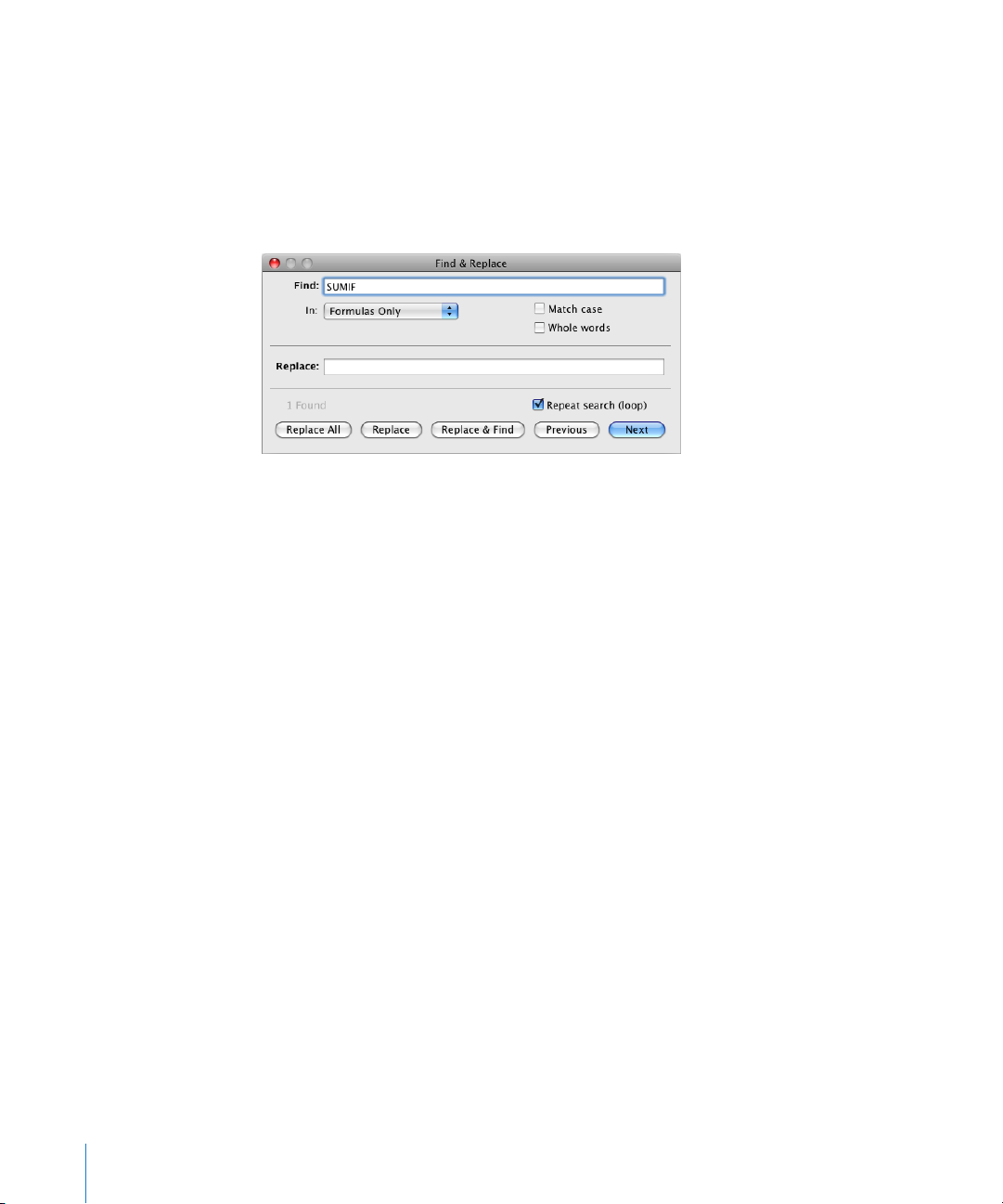
Finding and Replacing Formula Elements

In Numbers, using the Find & Replace window, you can search through all of a

spreadsheet’s formulas to nd and optionally change elements.

Here are ways to open the Find & Replace window:

Choose Edit > Find > Show Search, and then click Find & Replace. m

Choose View > Show Formula List, and then click Find & Replace. m

Find: Type the formula element (cell reference, operator, function, and so on) you

want to nd.

In: Choose Formulas Only from this pop-up menu.

Match case: Select to nd only elements whose uppercase and lowercase letters

match exactly what’s in the Find eld.

Whole words: Select to nd only elements whose entire contents match what’s in the Find eld.

Replace: Optionally type what you want to use to replace what’s in the Find eld.

Repeat search (loop): Select to continue looking for what’s in the Find eld even

after the entire spreadsheet has been searched.

Next or Previous: Click to search for the next or previous instance of what’s in the

Find eld. When an element is found, the Formula Editor opens and displays the

formula containing the instance of the element.

Replace All: Click to replace all instances of what’s in the Find eld with what’s in the Replace eld.

Replace: Click to replace the current instance of what’s in the Find eld with what’s in the Replace eld.

Replace & Find: Click to replace the current instance of what’s in the Find eld and to locate the next instance.

32 Chapter 1 Using Formulas in Tables

Overview of the iWork Functions

This chapter introduces the functions available in iWork.

An Introduction to Functions

A function is a named operation that you can include in a formula to perform a calculation or to manipulate data in a table cell.

iWork provides functions that do things such as perform mathematical or nancial

operations, retrieve cell values based on a search, manipulate strings of text, or get the current date and time. Each function has a name followed by one or more arguments enclosed in parentheses. You use arguments to provide the values that the function needs to perform its work.

For example, the following formula contains a function named SUM with a single argument (a range of cells) that adds the values in column A, rows 2 through 10:

=SUM(A2:A10)

The number and types of arguments vary for each function. The number and description of the arguments are included with the function in the alphabetical “Listing of Function Categories” on page 40. The descriptions also include additional information and examples for each function.

Information About Functions

For further information on Go to

Syntax used in function denitions “Syntax Elements and Terms Used In Function

Denitions” on page 34

Types of arguments that are used by functions “Value Types” on page 36

Categories of functions, such as duration and statistical

Arguments common to several nancial functions “Common Arguments Used in Financial

Supplemental examples and topics “Additional Examples and Topics Included” on

“Listing of Function Categories” on page 40. Functions are listed alphabetically within each category.

Functions” on page 341

page 340

Syntax Elements and Terms Used In Function Denitions

Functions are described using specic syntax elements and terms.

Term or symbol Meaning

uppercase text Function names are shown in all uppercase text.

However, a function name can be entered using any combination of uppercase or lowercase letters.

parentheses Function arguments are enclosed in parentheses.

Parentheses are required, although in limited

circumstances iWork can automatically insert the

nal closing parenthesis for you.

italic text Italic text indicates that you must replace the

argument name with a value the function will use to calculate a result. Arguments have a value type, such as “number,” “date/time,” or “string.” Value types are discussed in “Value Types” on page 36.

commas and semicolons The syntax descriptions for functions use commas

to separate arguments. If your Language and Text

preferences (Mac OS X version 10.6 or higher) or International preferences (earlier versions of Max OS X) are set up to use the comma as a decimal separator, separate arguments using a semicolon instead of a comma.

34 Chapter 2 Overview of the iWork Functions

Term or symbol Meaning

ellipsis (…) An argument followed by an ellipsis can be

repeated as many times as necessary. Any limitations are described in the argument

denition.

array An array is a sequence of values used by a

function, or returned by a function.

array constant An array constant is a set of values enclosed

within braces ({}) and is typed directly into the function. For example, {1, 2, 5, 7} or {“12/31/2008”, “3/15/2009”, “8/20/2010”}.

array function A small number of functions are described as

“array function,” meaning the function returns an array of values rather than a single value. These functions are commonly used to provide values to another function.

Boolean expression A Boolean expression is an expression that

evaluates to the Boolean value TRUE or FALSE.

constant A constant is a value specied directly within

the formula that contains no function calls or references. For example, in the formula =CONCATENATE(”cat”, “s”), “cat” and “s” are constants.

modal argument A modal argument is one that can have one of

several possible specied values. Usually, modal

arguments specify something about the type of calculation the function should perform or about the type of data the function should return. If a modal argument has a default value, it is

specied in the argument description.

condition A condition is an expression that can include

comparison operators, constants, the ampersand string operator, and references. The contents of the condition must be such that the result of comparing the condition to another value

results in the Boolean value TRUE or FALSE.

Further information and examples are included in “Specifying Conditions and Using Wildcards” on page 360.

Chapter 2 Overview of the iWork Functions 35

Value Types

A function argument has a type, which species what type of information the

argument can contain. Functions also return a value of a particular type.

Value Type Description

any If an argument is specied as “any,” it can be a

Boolean value, date/time value, duration value, number value, or string value.

Boolean A Boolean value is a logical TRUE (1) or FALSE

(0) value or a reference to a cell containing or

resulting in a logical TRUE or FALSE value. It is

generally the result of evaluating a Boolean

expression, but a Boolean value can be specied

directly as an argument to a function or as the content of a cell. A common use of a Boolean value is to determine which expression is to be returned by the IF function.

collection An argument that is specied as a collection can

be a reference to a single table cell range, an array constant, or an array returned by an array

function. An argument specied as collection will have an additional attribute dening the type of

values it can contain.

date/time This is a date/time value or a reference to a

cell containing a date/time value in any of the formats supported by iWork. If a date/time value is typed into the function, it should be enclosed

in quotation marks. You can choose to display

only a date or time in a cell, but all date/time values contain both a date and a time.

Although dates can usually be entered directly as strings (for example, “12/31/2010”), using the DATE function insures the date will be interpreted consistently regardless of the date format selected in System Preferences (search for “date format” in the System Preferences window).

36 Chapter 2 Overview of the iWork Functions

Value Type Description

duration A duration is a length of time or a reference

to a cell containing a length of time. Duration values consist of weeks (w or weeks), days (d or days), hours (h or hours), minutes (m or minutes), seconds (s or seconds), and milliseconds (ms or milliseconds). A duration value can be entered in one of two formats.

The rst format consists of a number, followed

by a time period (such as h for hours), optionally followed by a space, and is repeated for other time periods. You can use either the abbreviation for specifying the period, such as “h”, or the full name, such as “hours.” For example, 12h 5d 3m represents a duration of 12 hours, 5 days, and 3 minutes. TIme periods do not have to be entered

in order and spaces are not required. 5d 5h is the

same as 5h5d. If typed directly into a formula, the

string should be enclosed in quotation marks, as

in “12h 5d 3m”.

A duration can also be entered as a series of numbers delimited by colons. If this format is used, the seconds argument should be included and end with a decimal followed by the number of milliseconds, which can be 0, if the duration value could be confused with a date/time value. For example, 12:15:30.0 would represent a duration of 12 hours, 15 minutes, and 30 seconds, whereas 12:15:30 would be 12:15:30 a.m. 5:00.0 would represent a duration of exactly 5 minutes. If typed directly into a function, the string

should be enclosed in quotation marks, as in

“12:15:30.0” or “5:00.0”. If the cell is formatted to a particular duration display, the duration units are applied relative to that duration display and the

milliseconds need not be specied.

Chapter 2 Overview of the iWork Functions 37

Value Type Description

list A list is a comma-separated sequence of other

values. For example, =CHOOSE(3, “1st”, “second”, 7, “last”). In some cases, the list is enclosed in an additional set of parentheses. For example, =AREAS((B1:B5, C10:C12)).

modal A modal value is a single value, often a number,

representing a specic mode for a modal argument. “Modal argument” is dened in

“Syntax Elements and Terms Used In Function Denitions” on page 34.

number A number value is a number, a numeric

expression, or a reference to a cell containing a numeric expression. If the acceptable values of a number are limited (for example, the number must be greater than 0), this is included within the argument description.

range value A range value is a reference to a single range of

cells (can be a single cell). A range value will have

an additional attribute dening the type of values

it should contain. This will be included within the argument description.

38 Chapter 2 Overview of the iWork Functions

Value Type Description

reference This is a reference to a single cell or a range

of cells. If the range is more than one cell, the starting and ending cell are separated by a single colon. For example, =COUNT(A3:D7).

Unless the cell name is unique within all tables,

the reference must contain the name of the table if the reference is to a cell on another table. For example, =Table 2::B2. Note that the table name and cell reference are separated by a double colon (::).

If the table is on another sheet, the sheet name must also be included, unless the cell name is

unique within all the the sheets. For example,

=SUM(Sheet 2::Table 1::C2:G2). The sheet name, table name and cell reference are separated by double colons.

Some functions that accept ranges can operate on ranges that span multiple tables. Assume

that you have a le open that has one sheet

containing three tables (Table 1, Table 2, Table

3). Assume further that cell C2 in each table contains the number 1. The table-spanning formula =SUM(Table 1:Table 2 :: C2) would sum cell C2 in all tables between Table 1 and Table 2. So the result would be 2. If you drag Table 3 so that it appears between Table 1 and Table 2 in the sidebar, the function will return 3, since it is now summing cell C2 in all three tables (Table 3 is between Table 1 and Table 2).

string A string is zero or more characters, or a reference

to a cell containing one or more characters. The characters can consist of any printable characters, including numbers. If a string value is typed into

the formula, it must be enclosed in quotation

marks. If the string value is somehow limited (for example, the string must represent a date), this is included within the argument description.

Chapter 2 Overview of the iWork Functions 39

Listing of Function Categories

There are several categories of functions. For example, some functions perform

calculations on date/time values, logical functions give a Boolean (TRUE or FALSE) result, and other functions perform nancial calculations. Each of the categories of

functions is discussed in a separate chapter.

“Listing of Date and Time Functions” on page 42

“Listing of Duration Functions” on page 64

“Listing of Engineering Functions” on page 72

“Listing of Financial Functions” on page 96

“Listing of Logical and Information Functions” on page 15 5

“Listing of Numeric Functions” on page 167

“Listing of Reference Functions” on page 206

“Listing of Statistical Functions” on page 225

“Listing of Text Functions” on page 306

“Listing of Trigonometric Functions” on page 326

40 Chapter 2 Overview of the iWork Functions

Pasting from Examples in Help

Many of the examples in help can be copied and pasted directly into a table or, in Numbers, onto a blank canvas. There are two groups of examples which can be

copied from help and pasted into a table. The rst are individual examples included within help. All such examples begin with an equal sign (=). In the help for the HOUR

function, there are two such examples.

To use one of these examples, select the text beginning with the equal sign through

the end of the example.

Once this text is highlighted, you can copy it and then paste it into any cell in a table. An alternative to copy and paste is to drag the selection from the example and drop it onto any cell in a table.

The second kind of example that can be copied are example tables included within help. This is the help example table for ACCRINT.

To use an example table, select all the cells in the example table, including the rst row.

Once this text is highlighted, you can copy it and then paste it into any cell in a table or onto a blank canvas in a Numbers sheet. Drag and drop cannot be used for this type of example.

Chapter 2 Overview of the iWork Functions 41

Date and Time Functions

The date and time functions help you work with dates and times to solve problems such as nding the number of working days between two dates or nding the name of the day of the week a date will fall on.

Listing of Date and Time Functions

iWork includes these date and time functions for use with tables.

Function Description

“DATE” (page 44) The DATE function combines separate values for

year, month, and day and returns a date/time value. Although dates can usually be entered directly as strings (for example, “12/31/2010”), using the DATE function ensures the date will be interpreted consistently regardless of the date

format specied in System Preferences (search for

“date format” in the System Preferences window).

“DATEDIF” (page 45) The DATEDIF function returns the number of

days, months, or years between two dates.

“DATEVALUE” (page 47) The DATEVALUE function converts a date

text string and returns a date/time value. This function is provided for compatibility with other spreadsheet programs.

“DAY” (page 47) The DAY function returns the day of the month

for a given date/time value.

“DAYNAME” (page 48) The DAYNAME function returns the name of

the day of the week from a date/time value or a number. Day 1 is Sunday.

“DAYS360” (page 49) The DAYS360 function returns the number of

days between two dates based on twelve 30-day months and a 360-day year.

Function Description

“EDATE” (page 50) The EDATE function returns a date that is some

number of months before or after a given date.

“EOMONTH” (page 51 ) The EOMONTH function returns a date that is the

last day of the month some number of months before or after a given date.

“HOUR” (page 51 ) The HOUR function returns the hour for a given

date/time value.

“MINUTE” (page 52) The MINUTE function returns the minutes for a

given date/time value.

“MONTH” (page 53) The MONTH function returns the month for a

given date/time value.

“MONTHNAME” (page 54) The MONTHNAME function returns the name of

the month from a number. Month 1 is January.

“NETWORKDAYS” (page 54) The NETWORKDAYS function returns the number

of working days between two dates. Working

days exclude weekends and any other specied

dates.

“NOW” (page 55) The NOW function returns the current date/time

value from the system clock.

“SECOND” (page 56) The SECOND function returns the seconds for a

given date/time value.

“TIME” (page 56) The TIME function converts separate values for

hours, minutes, and seconds into a date/time value.

“TIMEVALUE” (page 57) The TIMEVALUE function returns the time as a

decimal fraction of a 24-hour day from a given date/time value or from a text string.

“TODAY” (page 58) The TODAY function returns the current system

date. The time is set to 12:00 a.m.

Chapter 3 Date and Time Functions 43

Function Description

“WEEKDAY” (page 59) The WEEKDAY function returns a number that is

the day of the week for a given date.

“WEEKNUM” (page 60) The WEEKNUM function returns the number of

the week within the year for a given date.

“WORKDAY” (page 61 ) The WORKDAY function returns the date that is

the given number of working days before or after a given date. Working days exclude weekends

and any other dates specically excluded.

“YEAR” (page 62) The YEAR function returns the year for a given

date/time value.

“YEARFRAC” (page 63) The YEARFRAC function nds the fraction of a

year represented by the number of whole days between two dates.

DATE

The DATE function combines separate values for year, month, and day and returns a date/time value. Although dates can usually be entered directly as strings (for example, “12/31/2010”), using the DATE function ensures the date will be interpreted consistently

regardless of the date format specied in System Preferences (search for “date format”

in the System Preferences window).

DATE(year, month, day)

Â year: The year to include in the value returned. year is a number value. The value

isn’t converted. If you specify 10, the year 10 is used, not the year 1910 or 2010.

Â month: The month to include in the value returned. month is a number and should

be in the range 1 to 12.

Â day: The day to include in the value returned. day is a number value and should be

in the range 1 to the number of days in month.

Examples

If A1 contains 2014, A2 contains 11, and A3 contains 10:

=DATE(A1, A2, A3) returns Nov 10, 2014, which is displayed according to the cell’s current format.

=DATE(A1, A3, A2) returns Oct 11, 2014.

=DATE(2012, 2, 14) returns Feb 14, 2012.

Related Topics

For related functions and additional information, see:

“DURATION” on page 70

44 Chapter 3 Date and Time Functions

“TIME” on page 56

“Listing of Date and Time Functions” on page 42

“Value Types” on page 36

“The Elements of Formulas” on page 15

“Using the Keyboard and Mouse to Create and Edit Formulas” on page 26

“Pasting from Examples in Help” on page 41

DATEDIF

The DATEDIF function returns the number of days, months, or years between two dates.

DATEDIF(start-date, end-date, calc-method)

Â start-date: The starting date. start-date is a date/time value.

Â end-date: The ending date. end-date is a date/time value.

Â calc-method: Species how to express the time dierence and how dates in

dierent years or months are handled.

“D”: Count the number of days between the start and end dates.

“M”: Count the number of months between the start and end dates.

“Y”: Count the number of years between the start and end dates.

“MD”: Count the days between the start and end dates, ignoring months and years.

The month in end-date is considered to be the month in start-date. If the starting day is after the ending day, the count starts from the ending day as if it were in the preceding month. The year of the end-date is used to check for a leap year.

“YM”: Count the number of whole months between the start and end dates, ignoring the year. If the starting month/day is before the ending month/day, the dates are treated as though they are in the same year. If the starting month/day is after the ending month/day, the dates are treated as though they are in consecutive years.

“YD”: Count the number of days between the start and end dates, ignoring the year. If the starting month/day is before the ending month/day, the dates are treated as though they are in the same year. If the starting month/day is after the ending month/day, the dates are treated as though they are in consecutive years.

Chapter 3 Date and Time Functions 45

Examples

If A1 contains the date/time value 4/6/88 and A2 contains the date/time value 10/30/06:

=DATEDIF(A1, A2, “D”) returns 6781, the number of days between April 6, 1988, and October 30, 2006.

=DATEDIF(A1, A2, “M”) returns 222, the number of whole months between April 6, 1988, and October 30, 2006.

=DATEDIF(A1, A2, “Y”) returns 18, the number of whole years between April 6, 1988, and October 30,

2006.

=DATEDIF(A1, A2, “MD”) returns 24, the number of days between the sixth day of a month and the thirtieth day of the same month.

=DATEDIF(A1, A2, “YM”) returns 6, the number of months between April and the following October in any year.

=DATEDIF(A1, A2, “YD”) returns 207, the number of days between April 6 and the following October 30 in any year.

=DATEDIF(”04/06/1988”, NOW(), “Y”) & “ years, “ & DATEDIF(”04/06/1988”, NOW(), “YM”) & “ months, and “ & DATEDIF(”04/06/1988”, NOW(), “MD”) & “ days” returns the current age of someone born on April 6,

1988.

Related Topics

For related functions and additional information, see:

“DAYS360” on page 49

“NETWORKDAYS” on page 54

“NOW” on page 55

“YEARFRAC” on page 63

“Listing of Date and Time Functions” on page 42

“Value Types” on page 36

“The Elements of Formulas” on page 15

“Using the Keyboard and Mouse to Create and Edit Formulas” on page 26

“Pasting from Examples in Help” on page 41

46 Chapter 3 Date and Time Functions

DATEVALUE

The DATEVALUE function converts a date text string and returns a date/time value. This

function is provided for compatibility with other spreadsheet programs.

DATEVALUE(date-text)

Â date-text: The date string to be converted. date-text is a string value. It must be a

date specied within quotations or a date/time value. If date-text is not a valid date, an error is returned.

Examples

If cell B1 contains the date/time value August 2, 1979 06:30:00 and cell C1 contains the string 10/16/2008:

=DATEVALUE(B1) returns Aug 2, 1979, and is treated as a date value if referenced in other formulas.

The value returned is formatted according to the current cell format. A cell formatted as Automatic

uses the date format specied in System Preferences (search for “date format” in the System

Preferences window).

=DATEVALUE(C1) returns Oct 16, 2008.

=DATEVALUE(“12/29/1974”) returns Dec 29, 1979.

Related Topics

For related functions and additional information, see:

“DATE” on page 44

“TIME” on page 56

“Listing of Date and Time Functions” on page 42

“Value Types” on page 36

“The Elements of Formulas” on page 15

“Using the Keyboard and Mouse to Create and Edit Formulas” on page 26

“Pasting from Examples in Help” on page 41

DAY

The DAY function returns the day of the month for a given date/time value.

DAY(date)

Â date: The date the function should use. date is a date/time value. The time portion

is ignored by this function.

Chapter 3 Date and Time Functions 47

Examples

=DAY(”4/6/88 11:59:22 PM”) returns 6.

=DAY(“5/12/2009”) returns 12.

Related Topics

For related functions and additional information, see:

“DAYNAME” on page 48

“HOUR” on page 51

“MINUTE” on page 52

“MONTH” on page 53

“SECOND” on page 56

“YEAR” on page 62

“Listing of Date and Time Functions” on page 42

“Value Types” on page 36

“The Elements of Formulas” on page 15

“Using the Keyboard and Mouse to Create and Edit Formulas” on page 26

“Pasting from Examples in Help” on page 41

DAYNAME

The DAYNAME function returns the name of the day of the week from a date/time value or a number. Day 1 is Sunday.

DAYNAME(day-num)

Â day-num: The desired day of the week. day-num is a date/time value, or number

value in the range 1 to 7. If day-num has a decimal portion, it is ignored.

Examples

If B1 contains the date/time value August 2, 1979 06:30:00, C1 contains the string 10/16/2008, and D1 contains 6:

=DAYNAME(B1) returns Thursday.

=DAYNAME(C1) returns Thursday.

=DAYNAME(D1) returns Friday.

=DAYNAME(“12/29/1974”) returns Sunday.

48 Chapter 3 Date and Time Functions

Related Topics

For related functions and additional information, see:

“DAY” on page 47

“MONTHNAME” on page 54

“WEEKDAY” on page 59

“Listing of Date and Time Functions” on page 42

“Value Types” on page 36

“The Elements of Formulas” on page 15

“Using the Keyboard and Mouse to Create and Edit Formulas” on page 26

“Pasting from Examples in Help” on page 41

DAYS360

The DAYS360 function returns the number of days between two dates based on twelve 30-day months and a 360-day year.

DAYS360(start-date, end-date, use-euro-method)

Â start-date: The starting date. start-date is a date/time value.

Â end-date: The ending date. end-date is a date/time value.

Â use-euro-method: An optional value that species whether to use the NASD or

European method for dates falling on the 31st of a month.

NASD method (0, FALSE, or omitted): Use the NASD method for dates falling on the 31st of a month.

EURO method (1 or TRUE): Use the European method for dates falling on the 31st of a month.

Examples

=DAYS360(”12/20/2008”, “3/31/2009”) returns 101d.

=DAYS360(”2/27/2008”, “3/31/2009”,0) returns 394d.

=DAYS360(”2/27/2008”, “3/31/2009”,1) returns 393d, as the European calculation method is used.

Related Topics

For related functions and additional information, see:

“DATEDIF” on page 45

“NETWORKDAYS” on page 54

Chapter 3 Date and Time Functions 49

“YEARFRAC” on page 63

“Listing of Date and Time Functions” on page 42

“Value Types” on page 36

“The Elements of Formulas” on page 15

“Using the Keyboard and Mouse to Create and Edit Formulas” on page 26

“Pasting from Examples in Help” on page 41

EDATE

The EDATE function returns a date that is some number of months before or after a given date.

EDATE(start-date, month-oset)

Â start-date: The starting date. start-date is a date/time value.

Â month-oset:The number of months before or after the starting date. month-oset

is a number value. A negative month-oset is used to specify a number of months before the starting date and a positive month-oset is used to specify a number of months after the starting date.

Examples

=EDATE(”1/15/2000”, 1) returns 2/15/2000, the date one month later.

=EDATE(”1/15/2000”, -24) returns 1/15/1998, the date 24 months earlier.

Related Topics

For related functions and additional information, see:

“EOMONTH” on page 51

“Listing of Date and Time Functions” on page 42

“Value Types” on page 36

“The Elements of Formulas” on page 15

“Using the Keyboard and Mouse to Create and Edit Formulas” on page 26

“Pasting from Examples in Help” on page 41

50 Chapter 3 Date and Time Functions

EOMONTH

The EOMONTH function returns a date that is the last day of the month some number of months before or after a given date.

EOMONTH(start-date, month-oset)

Â start-date: The starting date. start-date is a date/time value.

Â month-oset:The number of months before or after the starting date. month-oset

is a number value. A negative month-oset is used to specify a number of months before the starting date and a positive month-oset is used to specify a number of months after the starting date.

Examples

=EOMONTH(”5/15/2010”, 5) returns Oct 31, 2010, the last day of the month ve months after May 2010.

=EOMONTH(”5/15/2010”, -5) returns Dec 31, 2009, the last day of the month ve months before May

2010.

Related Topics

For related functions and additional information, see:

“EDATE” on page 50

“Listing of Date and Time Functions” on page 42

“Value Types” on page 36

“The Elements of Formulas” on page 15

“Using the Keyboard and Mouse to Create and Edit Formulas” on page 26

“Pasting from Examples in Help” on page 41

HOUR

The HOUR function returns the hour for a given date/time value.

HOUR(time)

Â time: The time the function should use. time is a date/time value. The date portion

is ignored by this function.

Usage Notes

The hour returned is in 24-hour format (0 is midnight, 23 is 11:00 p.m.). Â

Examples

=HOUR(NOW()) returns the current hour of the day.

=HOUR(”4/6/88 11:59:22 AM”) returns 11.

Chapter 3 Date and Time Functions 51

Related Topics

For related functions and additional information, see:

“DAY” on page 47

“MINUTE” on page 52

“MONTH” on page 53

“SECOND” on page 56

“YEAR” on page 62

“Listing of Date and Time Functions” on page 42

“Value Types” on page 36

“The Elements of Formulas” on page 15

“Using the Keyboard and Mouse to Create and Edit Formulas” on page 26

“Pasting from Examples in Help” on page 41

MINUTE

The MINUTE function returns the minutes for a given date/time value.

MINUTE(time)

Â time: The time the function should use. time is a date/time value. The date portion

is ignored by this function.

Example

=MINUTE(”4/6/88 11:59:22 AM”) returns 59.

Related Topics

For related functions and additional information, see:

“DAY” on page 47

“HOUR” on page 51

“MONTH” on page 53

“SECOND” on page 56

“YEAR” on page 62

“Listing of Date and Time Functions” on page 42

52 Chapter 3 Date and Time Functions

“Value Types” on page 36

“The Elements of Formulas” on page 15

“Using the Keyboard and Mouse to Create and Edit Formulas” on page 26

“Pasting from Examples in Help” on page 41

MONTH

The MONTH function returns the month for a given date/time value.

MONTH(date)

Â date: The date the function should use. date is a date/time value. The time portion

is ignored by this function.

Example

=MONTH(”April 6, 1988 11:59:22 AM”) returns 4.

Related Topics

For related functions and additional information, see:

“DAY” on page 47

“HOUR” on page 51

“MINUTE” on page 52

“MONTHNAME” on page 54

“SECOND” on page 56

“YEAR” on page 62

“Listing of Date and Time Functions” on page 42

“Value Types” on page 36

“The Elements of Formulas” on page 15

“Using the Keyboard and Mouse to Create and Edit Formulas” on page 26

“Pasting from Examples in Help” on page 41

Chapter 3 Date and Time Functions 53

MONTHNAME

The MONTHNAME function returns the name of the month from a number. Month 1 is January.

MONTHNAME(month-num)

Â month-num: The desired month. month-num is a number value and must be in the

range 1 to 12. If month-num has a decimal portion, it is ignored.

Examples

=MONTHNAME(9) returns September.

=MONTHNAME(6) returns June.

Related Topics

For related functions and additional information, see:

“DAYNAME” on page 48

“MONTH” on page 53

“WEEKDAY” on page 59

“Listing of Date and Time Functions” on page 42

“Value Types” on page 36

“The Elements of Formulas” on page 15

“Using the Keyboard and Mouse to Create and Edit Formulas” on page 26

“Pasting from Examples in Help” on page 41

NETWORKDAYS

The NETWORKDAYS function returns the number of working days between two dates.

Working days exclude weekends and any other specied dates.

NETWORKDAYS(start-date, end-date, exclude-dates)

Â start-date: The starting date. start-date is a date/time value.

Â end-date: The ending date. end-date is a date/time value.

Â exclude-dates: An optional collection of dates that should be excluded from the

count. exclude-dates is a collection containing date/time values.

Example

=NETWORKDAYS(”11/01/2009”, “11/30/2009”, {”11/11/2009”,”11/26/2009”}) returns 19d, the number of

working days in November 2009 excluding weekends and the two holidays specically excluded.

54 Chapter 3 Date and Time Functions

Related Topics

For related functions and additional information, see:

“DATEDIF” on page 45

“DAYS360” on page 49

“WORKDAY” on page 61

“YEARFRAC” on page 63

“Listing of Date and Time Functions” on page 42

“Value Types” on page 36

“The Elements of Formulas” on page 15

“Using the Keyboard and Mouse to Create and Edit Formulas” on page 26

“Pasting from Examples in Help” on page 41

NOW

The NOW function returns the current date/time value from the system clock.

NOW()

Usage Notes

The NOW function does not have any arguments. However, you must include the Â parentheses: =NOW().

Example

=NOW() returns October 4, 2008 10:47 am, if your le is updated on October 4, 2008, at 10:47 a.m.

Related Topics

For related functions and additional information, see:

“TODAY” on page 58

“Listing of Date and Time Functions” on page 42

“Value Types” on page 36

“The Elements of Formulas” on page 15

“Using the Keyboard and Mouse to Create and Edit Formulas” on page 26

“Pasting from Examples in Help” on page 41

Chapter 3 Date and Time Functions 55

SECOND

The SECOND function returns the seconds for a given date/time value.

SECOND(time)

Â time: The time the function should use. time is a date/time value. The date portion

is ignored by this function.

Example

=SECOND(”4/6/88 11:59:22 am”) returns 22.

Related Topics

For related functions and additional information, see:

“DAY” on page 47

“HOUR” on page 51

“MINUTE” on page 52

“Listing of Date and Time Functions” on page 42

“Value Types” on page 36

“The Elements of Formulas” on page 15

“Using the Keyboard and Mouse to Create and Edit Formulas” on page 26

“Pasting from Examples in Help” on page 41

TIME

The TIME function converts separate values for hours, minutes, and seconds into a date/time value.

TIME(hours, minutes, seconds)

Â hours: The number of hours to include in the value returned. hours is a number

value. If hours has a decimal portion, it is ignored.

Â minutes: The number of minutes to include in the value returned. minutes is a

number value. If minutes has a decimal portion, it is ignored.

Â seconds: The number of seconds to include in the value returned. seconds is a

number value. If seconds has a decimal portion, it is ignored.

Usage Notes

You can specify hour, minute, and second values greater than 24, 60, and 60, Â respectively. If the hours, minutes, and seconds add up to more than 24 hours, 24 hours are repeatedly subtracted until the value is less than 24 hours.

56 Chapter 3 Date and Time Functions

Examples

=TIME(12, 0, 0) returns 12:00 pm.

=TIME(16, 45, 30) returns 4:45 pm.

=TIME(0, 900, 0) returns 3:00 pm.

=TIME(60, 0, 0) returns 12:00 pm.

=TIME(4.25, 0, 0) returns 4:00 am.

Related Topics

For related functions and additional information, see:

“DATE” on page 44

“DATEVALUE” on page 47

“DURATION” on page 70

“Listing of Date and Time Functions” on page 42

“Value Types” on page 36

“The Elements of Formulas” on page 15

“Using the Keyboard and Mouse to Create and Edit Formulas” on page 26

“Pasting from Examples in Help” on page 41

TIMEVALUE

The TIMEVALUE function returns the time as a decimal fraction of a 24-hour day from a

given date/time value or from a text string.

TIMEVALUE(time)

Â time: The time the function should use. time is a date/time value. The date portion

is ignored by this function.

Examples

=TIMEVALUE(”4/6/88 12:00”) returns 0.5 (noon represents one-half of the day).

=TIMEVALUE(”12:00:59”) returns 0.5007 (rounded to four decimal places of accuracy).

=TIMEVALUE(”9:00 pm”) returns 0.875 (21 hours, or 9:00 p.m., divided by 24).

Related Topics

For related functions and additional information, see:

“Listing of Date and Time Functions” on page 42

Chapter 3 Date and Time Functions 57

“Value Types” on page 36

“The Elements of Formulas” on page 15

“Using the Keyboard and Mouse to Create and Edit Formulas” on page 26

“Pasting from Examples in Help” on page 41

TODAY

The TODAY function returns the current system date. The time is set to 12:00 a.m.

TODAY()

Usage Notes

The TODAY function does not have any arguments. However, you must include the Â parentheses: =TODAY().

The displayed date is updated every time you open or modify your le. Â

You can use the NOW function to get the current date and time and to format the Â cell to display both.

Example

=TODAY() returns Apr 6, 2008, when calculated on April 6, 2008.

Related Topics

For related functions and additional information, see:

“NOW” on page 55

“Listing of Date and Time Functions” on page 42

“Value Types” on page 36

“The Elements of Formulas” on page 15

“Using the Keyboard and Mouse to Create and Edit Formulas” on page 26

“Pasting from Examples in Help” on page 41

58 Chapter 3 Date and Time Functions

WEEKDAY

The WEEKDAY function returns a number that is the day of the week for a given date.

WEEKDAY(date, rst-day)

Â date: The date the function should use. date is a date/time value. The time portion

is ignored by this function.

Â rst-day:An optional value that species how days are numbered.

Sunday is 1 (1 or omitted): Sunday is the rst day (day 1) of the week and Saturday

is day 7.

Monday is 1 (2): Monday is the rst day (day 1) of the week and Sunday is day 7.

Monday is 0 (3): Monday is the rst day (day 0) of the week and Sunday is day 6.

Examples

=WEEKDAY(”Apr 6, 1988”, 1) returns 4 (Wednesday, the fourth day if you start counting Sunday as day

1).

=WEEKDAY(”Apr 6, 1988”) returns the same value as the preceding example (numbering scheme 1 is

used if no number-scheme argument is specied).

=WEEKDAY(”Apr 6, 1988”, 2) returns 3 (Wednesday, the third day if you start counting Monday as day

1).

=WEEKDAY(”Apr 6, 1988”, 3) returns 2 (Wednesday, day number 2 if you start counting Monday as day

0).

Related Topics

For related functions and additional information, see:

“DAYNAME” on page 48

“MONTHNAME” on page 54

“Listing of Date and Time Functions” on page 42

“Value Types” on page 36

“The Elements of Formulas” on page 15

“Using the Keyboard and Mouse to Create and Edit Formulas” on page 26

“Pasting from Examples in Help” on page 41

Chapter 3 Date and Time Functions 59

WEEKNUM

The WEEKNUM function returns the number of the week within the year for a given date.

WEEKNUM(date, rst-day)

Â date: The date the function should use. date is a date/time value. The time portion

is ignored by this function.

Â rst-day:An optional value that species whether weeks should begin on Sunday

or Monday.

Sunday is 1 (1 or omitted): Sunday is the rst day (day 1) of the week and Saturday

is day 7.

Monday is 1 (2): Monday is the rst day (day 1) of the week and Sunday is day 7.

Example

=WEEKNUM(”7/12/2009”,1) returns 29.

=WEEKNUM(”7/12/2009”,2) returns 28.

Related Topics

For related functions and additional information, see:

“DAY” on page 47

“HOUR” on page 51

“MINUTE” on page 52

“MONTH” on page 53

“SECOND” on page 56

“YEAR” on page 62

“Listing of Date and Time Functions” on page 42

“Value Types” on page 36

“The Elements of Formulas” on page 15

“Using the Keyboard and Mouse to Create and Edit Formulas” on page 26

“Pasting from Examples in Help” on page 41

60 Chapter 3 Date and Time Functions

WORKDAY

The WORKDAY function returns the date that is the given number of working days before or after a given date. Working days exclude weekends and any other dates

specically excluded.

WORKDAY(date, work-days, exclude-dates)

Â date: The date the function should use. date is a date/time value. The time portion

is ignored by this function.

Â work-days: The number of working days before or after the given date. work-days

is a number value. It is positive if the desired date is after date and negative if the desired date is before date.

Â exclude-dates: An optional collection of dates that should be excluded from the

count. exclude-dates is a collection containing date/time values.

Example

=WORKDAY(”11/01/2009”, 20, {”11/11/2009”,”11/26/2009”}) returns Dec 1, 2009, the work day 20 days

after 11/01/2009 excluding weekends and the two holidays specically excluded.

Related Topics

For related functions and additional information, see:

“NETWORKDAYS” on page 54

“Listing of Date and Time Functions” on page 42

“Value Types” on page 36

“The Elements of Formulas” on page 15

“Using the Keyboard and Mouse to Create and Edit Formulas” on page 26

“Pasting from Examples in Help” on page 41

Chapter 3 Date and Time Functions 61

YEAR

The YEAR function returns the year for a given date/time value.

YEAR(date)

Â date: The date the function should use. date is a date/time value. The time portion

is ignored by this function.

Examples

=YEAR(”April 6, 2008”) returns 2008.

=YEAR(NOW()) returns 2009 when evaluated on June 4, 2009.

Related Topics

For related functions and additional information, see:

“DAY” on page 47

“HOUR” on page 51

“MINUTE” on page 52

“MONTH” on page 53

“SECOND” on page 56

“Listing of Date and Time Functions” on page 42

“Value Types” on page 36

“The Elements of Formulas” on page 15

“Using the Keyboard and Mouse to Create and Edit Formulas” on page 26

“Pasting from Examples in Help” on page 41

62 Chapter 3 Date and Time Functions

YEARFRAC

The YEARFRAC function nds the fraction of a year represented by the number of

whole days between two dates.

YEARFRAC(start-date, end-date, days-basis)

Â start-date: The starting date. start-date is a date/time value.

Â end-date: The ending date. end-date is a date/time value.

Â days-basis: An optional argument specifying the number of days per month and

days per year used in the calculations.

30/360 (0 or omitted): 30 days in a month, 360 days in a year, using the NASD method for dates falling on the 31st of a month.

actual/actual (1): Actual days in each month, actual days in each year.

actual/360 (2): Actual days in each month, 360 days in a year.

actual/365 (3): Actual days in each month, 365 days in a year.

30E/360 (4): 30 days in a month, 360 days in a year, using the European method for

dates falling on the 31st of a month (European 30/360).

Examples

=YEARFRAC(”12/15/2009”, “6/30/2010”,0) returns 0.541666667.

=YEARFRAC(”12/15/2009”, “6/30/2010”,1) returns 0.539726027.

=YEARFRAC(”12/15/2009”, “6/30/2010”,2) returns 0.547222222.

=YEARFRAC(”12/15/2009”, “6/30/2010”,3) returns 0.539726027.

=YEARFRAC(”12/15/2009”, “6/30/2010”,4) returns 0.541666667.

Related Topics

For related functions and additional information, see:

“DATEDIF” on page 45

“DAYS360” on page 49

“NETWORKDAYS” on page 54

“Listing of Date and Time Functions” on page 42

“Value Types” on page 36

“The Elements of Formulas” on page 15

“Using the Keyboard and Mouse to Create and Edit Formulas” on page 26

“Pasting from Examples in Help” on page 41

Chapter 3 Date and Time Functions 63

Duration Functions

The duration functions help you work with periods of time (durations) by converting between dierent time periods, such as hours, days, and weeks.

Listing of Duration Functions

iWork provides these duration functions for use with tables.

Function Description

“DUR2DAYS” (page 65) The DUR2DAYS function converts a duration

value to a number of days.

“DUR2HOURS” (page 65) The DUR2HOURS function converts a duration

value to a number of hours.

“DUR2MILLISECONDS” (page 66) The DUR2MILLISECONDS function converts a

duration value to a number of milliseconds.

“DUR2MINUTES” (page 67) The DUR2MINUTES function converts a duration

value to a number of minutes.

“DUR2SECONDS” (page 68) The DUR2SECONDS function converts a duration

value to a number of seconds.

“DUR2WEEKS” (page 69) The DUR2WEEKS function converts a duration

value to a number of weeks.

“DURATION” (page 70) The DURATION function combines separate

values for weeks, days, hours, minutes, seconds, and milliseconds and returns a duration value.

“STRIPDURATION” (page 71 ) The STRIPDURATION function evaluates a given

value and returns either the number of days represented, if a duration value, or the given value. This function is included for compatibility with other spreadsheet applications.

DUR2DAYS

The DUR2DAYS function converts a duration value to a number of days.

DUR2DAYS(duration)

Â duration: The length of time to be converted. duration is a duration value.

Examples

=DUR2DAYS(”2w 3d 2h 10m 0s 5ms”) returns 17.09027784.

=DUR2DAYS(”10:0:13:00:05.500”) returns 70.5417302.

Related Topics

For related functions and additional information, see:

“DUR2HOURS” on page 65

“DUR2MILLISECONDS” on page 66

“DUR2MINUTES” on page 67

“DUR2SECONDS” on page 68

“DUR2WEEKS” on page 69

“Listing of Duration Functions” on page 64

“Value Types” on page 36

“The Elements of Formulas” on page 15

“Using the Keyboard and Mouse to Create and Edit Formulas” on page 26

“Pasting from Examples in Help” on page 41

DUR2HOURS

The DUR2HOURS function converts a duration value to a number of hours.

DUR2HOURS(duration)

Â duration: The length of time to be converted. duration is a duration value.

Examples

=DUR2HOURS(”2w 3d 2h 10m 0s 5ms”) returns 410.1666681.

=DUR2HOURS(”10:0:13:00:05.500”) returns 1693.001528.

Chapter 4 Duration Functions 65

Related Topics

For related functions and additional information, see:

“DUR2DAYS” on page 65

“DUR2MILLISECONDS” on page 66

“DUR2MINUTES” on page 67

“DUR2SECONDS” on page 68

“DUR2WEEKS” on page 69

“Listing of Duration Functions” on page 64

“Value Types” on page 36

“The Elements of Formulas” on page 15

“Using the Keyboard and Mouse to Create and Edit Formulas” on page 26

“Pasting from Examples in Help” on page 41

DUR2MILLISECONDS

The DUR2MILLISECONDS function converts a duration value to a number of milliseconds.

DUR2MILLISECONDS(duration)

Â duration: The length of time to be converted. duration is a duration value.

Examples

=DUR2MILLISECONDS(”2w 3d 2h 10m 0s 5ms”) returns 1476600005.

=DUR2MILLISECONDS(”10:0:13:00:05.500”) returns 6094805500.

Related Topics

For related functions and additional information, see:

“DUR2DAYS” on page 65

“DUR2HOURS” on page 65

“DUR2MINUTES” on page 67

“DUR2SECONDS” on page 68

“DUR2WEEKS” on page 69

“Listing of Duration Functions” on page 64

66 Chapter 4 Duration Functions

“Value Types” on page 36

“The Elements of Formulas” on page 15

“Using the Keyboard and Mouse to Create and Edit Formulas” on page 26

“Pasting from Examples in Help” on page 41

DUR2MINUTES

The DUR2MINUTES function converts a duration value to a number of minutes.

DUR2MINUTES(duration)

Â duration: The length of time to be converted. duration is a duration value.

Examples

=DUR2MINUTES(”2w 3d 2h 10m 0s 5ms”) returns 24610.0000833333.

=DUR2MINUTES(”10:0:13:00:05.500”) returns 101580.091666667.

Related Topics

For related functions and additional information, see:

“DUR2DAYS” on page 65

“DUR2HOURS” on page 65

“DUR2MILLISECONDS” on page 66

“DUR2SECONDS” on page 68

“DUR2WEEKS” on page 69

“Listing of Duration Functions” on page 64

“Value Types” on page 36

“The Elements of Formulas” on page 15

“Using the Keyboard and Mouse to Create and Edit Formulas” on page 26

“Pasting from Examples in Help” on page 41

Chapter 4 Duration Functions 67

DUR2SECONDS

The DUR2SECONDS function converts a duration value to a number of seconds.

DUR2SECONDS(duration)

Â duration: The length of time to be converted. duration is a duration value.

Examples

=DUR2SECONDS(”2w 3d 2h 10m 0s 5ms”) returns 1476600.005.

=DUR2SECONDS(”10:0:13:00:05.500”) returns 6094805.5.

Related Topics

For related functions and additional information, see:

“DUR2DAYS” on page 65

“DUR2HOURS” on page 65

“DUR2MILLISECONDS” on page 66

“DUR2MINUTES” on page 67

“DUR2WEEKS” on page 69

“Listing of Duration Functions” on page 64

“Value Types” on page 36

“The Elements of Formulas” on page 15

“Using the Keyboard and Mouse to Create and Edit Formulas” on page 26

“Pasting from Examples in Help” on page 41

68 Chapter 4 Duration Functions

DUR2WEEKS

The DUR2WEEKS function converts a duration value to a number of weeks.

DUR2WEEKS(duration)

Â duration: The length of time to be converted. duration is a duration value.

Examples

=DUR2WEEKS(”2w 3d 2h 10m 0s 5ms”) returns 2.44146826223545.

=DUR2WEEKS(”10:0:13:00:05.500”) returns 10.0773900462963.

Related Topics

For related functions and additional information, see:

“DUR2DAYS” on page 65

“DUR2HOURS” on page 65

“DUR2MILLISECONDS” on page 66

“DUR2MINUTES” on page 67

“DUR2SECONDS” on page 68

“Listing of Duration Functions” on page 64

“Value Types” on page 36

“The Elements of Formulas” on page 15

“Using the Keyboard and Mouse to Create and Edit Formulas” on page 26

“Pasting from Examples in Help” on page 41

Chapter 4 Duration Functions 69

DURATION

The DURATION function combines separate values for weeks, days, hours, minutes, seconds, and milliseconds and returns a duration value.

DURATION(weeks, days, hours, minutes, seconds, milliseconds)

Â weeks: A value representing the number of weeks. weeks is a number value.

Â days: An optional value representing the number of days. days is a number value.

Â hours: An optional value representing the number of hours. hours is a number value.

Â minutes: An optional value representing the number of minutes. minutes is a

number value.

Â seconds: An optional value representing the number of seconds. seconds is a

number value.

Â milliseconds: An optional value representing the number of milliseconds.

milliseconds is a number value.

Usage Notes

An argument that is 0 can be omitted, but the comma must be included if later Â values are included. For example, =DURATION(, ,12, 3) would return a duration value of 12h 3m (12 hours and 3 minutes).

Negative values are permitted. For example, =DURATION(0, 2, -24) would return a Â duration of 1 day (2 days minus 24 hours).

Examples

=DURATION(1) returns 1w (1 week).

=DURATION(,,1) returns 1h (1 hour).

=DURATION(1.5) returns 1w 3d 12h (1 week, 3 days, 12 hours or 1.5 weeks).

=DURATION(3, 2, 7, 10, 15.3505) returns 3w 2d 7h 10m 15s 350ms (3 weeks, 2 days, 7 hours, 10 minutes, 15 seconds, 350 milliseconds).

Related Topics

For related functions and additional information, see:

“DATE” on page 44

“TIME” on page 56

“Listing of Duration Functions” on page 64

“Value Types” on page 36

“The Elements of Formulas” on page 15

“Using the Keyboard and Mouse to Create and Edit Formulas” on page 26

“Pasting from Examples in Help” on page 41

70 Chapter 4 Duration Functions

STRIPDURATION

The STRIPDURATION function evaluates a given value and returns either the number of days represented, if a duration value, or the given value. This function is included for compatibility with other spreadsheet applications.

STRIPDURATION(any-value)

Â any-value: A value. any-value can contain any value type.

Usage Notes

If Â any-value is a duration value, the result is the same as for DUR2DAYS; otherwise any-value is returned.

This function may be automatically inserted when a Numbers ’08 document is Â upgraded, or an Excel or Appleworks document is imported. It is removed in any

copy of the le saved as a Numbers ’08 or Excel document.

Examples

=STRIPDURATION(”1w”) returns 7, the equivalent of one week in days.

=STRIPDURATION(12) returns 12; since it was not a duration value it is returned.

=STRIPDURATION (”abc”) returns “abc”.

Related Topics

For related functions and additional information, see:

“Listing of Duration Functions” on page 64

“Value Types” on page 36

“The Elements of Formulas” on page 15

“Using the Keyboard and Mouse to Create and Edit Formulas” on page 26

“Pasting from Examples in Help” on page 41

Chapter 4 Duration Functions 71

Engineering Functions

The engineering functions help you calculate some common engineering values and convert between dierent numeric

bases.

Listing of Engineering Functions

iWork provides these engineering functions for use with tables.

Function Description

“BASETONUM” (page 73) The BASETONUM function converts a number of

the specied base into a number in base 10.

“BESSELJ” (page 74) The BESSELJ function returns the integer Bessel

function J

“BESSELY” (page 75) The BESSELY function returns the integer Bessel

function Y

“BIN2DEC” (page 76) The BIN2DEC function converts a binary number

to the corresponding decimal number.

“BIN2HEX” (page 77) The BIN2HEX function converts a binary number

to the corresponding hexadecimal number.

“BIN2OCT” (page 78) The BIN2OCT function converts a binary number

to the corresponding octal number.

“CONVERT” (page 79) The CONVERT function converts a number from

one measurement system to its corresponding value in another measurement system.

“DEC2BIN” (page 83) The DEC2BIN function converts a decimal

number to the corresponding binary number.

“DEC2HEX” (page 84) The DEC2HEX function converts a decimal

number to the corresponding hexadecimal number.

(x).

Function Description

“DEC2OCT” (page 85) The DEC2OCT function converts a decimal

number to the corresponding octal number.

“DELTA” (page 86) The DELTA function determines whether two

values are exactly equal.

“ERF” (page 87) The ERF function returns the error function

integrated between two values.

“ERFC” (page 87) The ERFC function returns the complementary

ERF function integrated between a given lower

bound and innity.

“GESTEP” (page 88) The GESTEP function determines if one value is

greater than or exactly equal to another value.

“HEX2BIN” (page 89) The HEX2BIN function converts a hexadecimal

number to the corresponding binary number.

“HEX2DEC” (page 90) The HEX2DEC function converts a hexadecimal

number to the corresponding decimal number.

“HEX2OCT” (page 91) The HEX2OCT function converts a hexadecimal

number to the corresponding octal number.

“NUMTOBASE” (page 92) The NUMTOBASE function converts a number

from base 10 into a number in the specied base.

“OCT2BIN” (page 93) The OCT2BIN function converts an octal number

to the corresponding binary number.

“OCT2DEC” (page 94) The OCT2DEC function converts an octal number

to the corresponding decimal number.

“OCT2HEX” (page 95) The OCT2HEX function converts an octal number

to the corresponding hexadecimal number.

BASETONUM

The BASETONUM function converts a number of the specied base into a number in base 10.

BASETONUM(convert-string, base)

Â convert-string: The string representing the number to be converted. convert-string

is a string value. It must contain only numbers and letters that apply in the base of the number being converted.

Â base: The current base of the number to be converted. base is a number value and

must be in the range 1 to 36.

Chapter 5 Engineering Functions 73

Usage Notes

This function returns a number value and can properly be used in a formula Â containing other number values. Some other spreadsheet applications return a string value.

Examples

=BASETONUM(”3f”, 16) returns 63.

=BASETONUM(1000100, 2) returns 68.

=BASETONUM(”7279”, 8) returns an error, since the digit “9” is not valid in base 8.

Related Topics

For related functions and additional information, see:

“BIN2DEC” on page 76

“HEX2DEC” on page 90

“NUMTOBASE” on page 92

“OCT2DEC” on page 94

“Listing of Engineering Functions” on page 72

“Value Types” on page 36

“The Elements of Formulas” on page 15

“Using the Keyboard and Mouse to Create and Edit Formulas” on page 26

“Pasting from Examples in Help” on page 41

BESSELJ

The BESSELJ function returns the integer Bessel function Jn(x).

BESSELJ(any-x-value, n-value)

Â any-x-value: The x value at which you want to evaluate the function. any-x-value is

a number value.

Â n-value: The order of the function. n-value is a number value and must be greater

than or equal to 0. If n-value has a decimal portion, it is ignored.

Examples

=BESSELJ(25, 3) returns 0.108343081061509.

=BESSELJ(25, 3.9) also returns 0.108343081061509, since any decimal portion of n-value is ignored.

=BESSELJ(-25, 3) returns -0.108343081061509.

74 Chapter 5 Engineering Functions

Related Topics

For related functions and additional information, see:

“BESSELY” on page 75

“Listing of Engineering Functions” on page 72

“Value Types” on page 36

“The Elements of Formulas” on page 15

“Using the Keyboard and Mouse to Create and Edit Formulas” on page 26

“Pasting from Examples in Help” on page 41

BESSELY

The BESSELY function returns the integer Bessel function Yn(x).

BESSELY(pos-x-value, n-value)

Â pos-x-value: The positive x value at which you want to evaluate the function.

pos-x-value is a number value and must be greater than 0.

Â n-value: The order of the function. n-value is a number value and must be greater

than or equal to 0. If n-value has a decimal portion, it is ignored.

Usage Notes

This form of the Bessel function is also known as the Neumann function. Â

Examples

=BESSELY(25, 3) returns 0.117924850396893.

=BESSELY(25, 3.9) also returns 0.117924850396893, since any decimal portion of n-value is ignored.

=BESSELY(-25, 3) returns an error, since negative or zero values are not permitted.

Related Topics

For related functions and additional information, see:

“BESSELJ” on page 74

“Listing of Engineering Functions” on page 72

“Value Types” on page 36

“The Elements of Formulas” on page 15

“Using the Keyboard and Mouse to Create and Edit Formulas” on page 26

“Pasting from Examples in Help” on page 41

Chapter 5 Engineering Functions 75

BIN2DEC

The BIN2DEC function converts a binary number to the corresponding decimal number.

BIN2DEC(binary-string, convert-length)

Â binary-string: The string representing the number to be converted. binary-string is

a string value. It must contain only 0s and 1s.

Â convert-length: An optional value specifying minimum length of the number

returned. convert-length is a number value and must be in the range 1 to 32. If omitted, it is assumed to be 1. If included, convert-string is padded with leading zeros, if necessary, so that it is at least the length specied by convert-length.

Examples

=BIN2DEC(”1001”) returns 9.

=BIN2DEC(”100111”, 3) returns 039.

=BIN2DEC(101101) returns 45.

Related Topics

For related functions and additional information, see:

“BIN2HEX” on page 77

“BIN2OCT” on page 78

“DEC2BIN” on page 83

“HEX2DEC” on page 90

“OCT2DEC” on page 94

“Listing of Engineering Functions” on page 72

“Value Types” on page 36

“The Elements of Formulas” on page 15

“Using the Keyboard and Mouse to Create and Edit Formulas” on page 26

“Pasting from Examples in Help” on page 41

76 Chapter 5 Engineering Functions

BIN2HEX

The BIN2HEX function converts a binary number to the corresponding hexadecimal number.

BIN2HEX(binary-string, convert-length)

Â binary-string: The string representing the number to be converted. binary-string is

a string value. It must contain only 0s and 1s.

Â convert-length: An optional value specifying minimum length of the number

Usage Notes

This function uses two’s complement notation, based on 32 bits. Therefore, negative Â numbers will always be 8 digits in length.

Examples

=BIN2HEX(”100101”) returns 25.

=BIN2HEX(”100111”, 3) returns 027.

=BIN2HEX(101101) returns 2D.

Related Topics

For related functions and additional information, see:

“BIN2DEC” on page 76

“BIN2OCT” on page 78

“DEC2HEX” on page 84

“HEX2BIN” on page 89

“OCT2HEX” on page 95

“Listing of Engineering Functions” on page 72

“Value Types” on page 36

“The Elements of Formulas” on page 15

“Using the Keyboard and Mouse to Create and Edit Formulas” on page 26

“Pasting from Examples in Help” on page 41

Chapter 5 Engineering Functions 77

BIN2OCT

The BIN2OCT function converts a binary number to the corresponding octal number.

BIN2OCT(binary-string, convert-length)

Â binary-string: The string representing the number to be converted. binary-string is

a string value. It must contain only 0s and 1s.

Â convert-length: An optional value specifying minimum length of the number

Usage Notes

This function uses two’s complement notation, based on 32 bits. Therefore, negative Â numbers will always be 11 digits in length.

Examples

=BIN2OCT(”10011”) returns 23.

=BIN2OCT(”100111”, 3) returns 047.

Related Topics

For related functions and additional information, see:

“BIN2HEX” on page 77

“DEC2OCT” on page 85

“HEX2OCT” on page 91

“OCT2BIN” on page 93

“BIN2DEC” on page 76

“Listing of Engineering Functions” on page 72

“Value Types” on page 36

“The Elements of Formulas” on page 15

“Using the Keyboard and Mouse to Create and Edit Formulas” on page 26

“Pasting from Examples in Help” on page 41

78 Chapter 5 Engineering Functions

CONVERT

The CONVERT function converts a number from one measurement system to its corresponding value in another measurement system.

CONVERT(convert-num, from-unit, to-unit)

Â convert-num: The number to be converted. convert-num is a number value.

Â from-unit: The current unit of the number to be converted. from-unit is a string

value. It must be one of the specied constants.

Â to-unit: The new unit of the number to be converted. to-unit is a string value.

It must be one of the specied constants.

Usage Notes

The possible values for Â from-unit and to-unit are contained in tables that follow the examples (“Supported Conversion Units” on page 80). The tables are organized by category. If the value is entered into a referenced cell, instead of being typed

directly into the function, the quotes included in the tables are not required. Case is

important and must be strictly followed.

Examples

=CONVERT(9, “lbm”, “kg”) returns 4.08233133 (9 pounds is approximately 4.08 kilograms).

=CONVERT (26.2, “mi”, “m”) returns 42164.8128 (26.2 miles is approximately 42,164.8 meters).

=CONVERT(1, “tsp”, “ml”) returns 4.92892159375 (1 teaspoon is approximately 4.9 milliliters).

Related Topics

For related functions and additional information, see:

“Listing of Engineering Functions” on page 72

“Value Types” on page 36

“The Elements of Formulas” on page 15

“Using the Keyboard and Mouse to Create and Edit Formulas” on page 26

“Pasting from Examples in Help” on page 41

Chapter 5 Engineering Functions 79

Supported Conversion Units

Weight and mass

Measure Constant

Gram “g” (can be used with metric prexes)

Slug “sg”

Pound mass (avoirdupois) “lbm”

U (atomic mass unit) “u” (can be used with metric prexes)

Ounce mass (avoirdupois) “ozm”

Distance

Measure Constant

Meter “m” (can be used with metric prexes)

Statute mile “mi”

Nautical mile “Nmi”

Inch “in”

Foot “ft”

Yar d “yd”

Angstrom “ang” (can be used with metric prexes)

Pica (1/6 in., Postscript Pica) “Pica”

Duration

Measure Constant

Year “yr”

Week “wk”

Day “day”

Hour “hr”

Minute “mn”

Second “sec” (can be used with metric prexes)

80 Chapter 5 Engineering Functions

Speed

Measure Constant

Miles per hour “mi/h”

Miles per minute “mi/mn”

Meters per hour “m/h” (can be used with metric prexes)

Meters per minute “m/mn” (can be used with metric prexes)

Meters per second “m/s” (can be used with metric prexes)

Feet per minute “ft/mn”

Feet per second “ft/s”

Knot “kt”

Pressure

Measure Constant

Pascal “Pa” (can be used with metric prexes)

Atmosphere “atm” (can be used with metric prexes)

Millimeters of mercury “mmHg” (can be used with metric prexes)

Force

Measure Constant

Newton “N” (can be used with metric prexes)

Dyne “dyn” (can be used with metric prexes)

Pound force “lbf”

Energy

Measure Constant

Joule “J” (can be used with metric prexes)

Erg “e” (can be used with metric prexes)

Thermodynamic calorie “c” (can be used with metric prexes)

IT calorie “cal” (can be used with metric prexes)

Electron volt “eV” (can be used with metric prexes)

Horsepower-hour “HPh”

Chapter 5 Engineering Functions 81

Measure Constant

Watt-hour “Wh” (can be used with metric prexes)

Foot-pound “b”

BTU “BTU”

Power

Measure Constant

Horsepower “HP”

Watt “W” (can be used with metric prexes)

Magnetism

Measure Constant

Tesla “T” (can be used with metric prexes)

Gauss “ga” (can be used with metric prexes)

Temperature

Measure Constant

Degrees Celsius “C”

Degrees Fahrenheit “F”

Kelvins “K” (can be used with metric prexes)

Liquid

Measure Constant

Teaspoon “tsp”

Tablespoon “tbs”

Fluid ounce “oz”

Cup “cup”

U.S. pint “pt”

U.K. pint “uk_pt”

Quart “qt”

Gallon “gal”

Liter “l” (can be used with metric prexes)

82 Chapter 5 Engineering Functions

Metricprexes

Measure Constant Multiplier

exa “E” 1E+18

peta “P” 1E+15

tera “T” 1E+12

giga “G” 1E+09

mega “M” 1E+06

kilo “k” 1E+03

hecto “h” 1E+02

deca “e ” 1E+01

deci “d” 1E-01

centi “c” 1E-02

milli “m” 1E-03

micro “u” or “µ” 1E-06

nano “n” 1E-09

pico “p” 1E-12

femto “f” 1E-15

atto “a” 1E-18

Usage Notes

These prexes can only be used with the metric constants “g”, “u”, “m”, “ang”, “sec”, “m/h”, Â

“m/mn”, “m/s”, “Pa”, “atm”, “mmHg”, “N”, “dyn”, “J”, “e”, “c”, “cal”, “eV”, “Wh”, “W”, “T”, “ga”, “K”, and “l”.

DEC2BIN

The DEC2BIN function converts a decimal number to the corresponding binary number.

DEC2BIN(decimal-string, convert-length)

Â decimal-string: The string representing the number to be converted. decimal-string

is a string value. It must contain only the numbers 0 through 9.

Â convert-length: An optional value specifying minimum length of the number

Chapter 5 Engineering Functions 83

Examples

=DEC2BIN(100) returns 01100100.

=DEC2BIN(”1001”, 12) returns 001111101001.

Related Topics

For related functions and additional information, see:

“BIN2DEC” on page 76

“DEC2HEX” on page 84

“DEC2OCT” on page 85

“HEX2BIN” on page 89

“OCT2BIN” on page 93

“Listing of Engineering Functions” on page 72

“Value Types” on page 36

“The Elements of Formulas” on page 15

“Using the Keyboard and Mouse to Create and Edit Formulas” on page 26

“Pasting from Examples in Help” on page 41

DEC2HEX

The DEC2HEX function converts a decimal number to the corresponding hexadecimal number.

DEC2HEX(decimal-string, convert-length)

Â decimal-string: The string representing the number to be converted. decimal-string

is a string value. It must contain only the numbers 0 through 9.

Â convert-length: An optional value specifying minimum length of the number

Examples

=DEC2HEX(100) returns 64.

=DEC2HEX(”1001”, 4) returns 03E9.

84 Chapter 5 Engineering Functions

Related Topics

For related functions and additional information, see:

“BIN2HEX” on page 77

“DEC2BIN” on page 83

“DEC2OCT” on page 85

“HEX2DEC” on page 90

“OCT2HEX” on page 95

“Listing of Engineering Functions” on page 72

“Value Types” on page 36

“The Elements of Formulas” on page 15

“Using the Keyboard and Mouse to Create and Edit Formulas” on page 26

“Pasting from Examples in Help” on page 41

DEC2OCT

The DEC2OCT function converts a decimal number to the corresponding octal number.

DEC2OCT(decimal-string, convert-length)

Â decimal-string: The string representing the number to be converted. decimal-string

is a string value. It must contain only the numbers 0 through 9.

Â convert-length: An optional value specifying minimum length of the number

Examples

=DEC2OCT(100) returns 144.

=DEC2OCT(”1001”, 4) returns 1751.

Related Topics

For related functions and additional information, see:

“BIN2OCT” on page 78

“DEC2BIN” on page 83

“DEC2HEX” on page 84

Chapter 5 Engineering Functions 85

“HEX2OCT” on page 91

“OCT2DEC” on page 94

“Listing of Engineering Functions” on page 72

“Value Types” on page 36

“The Elements of Formulas” on page 15

“Using the Keyboard and Mouse to Create and Edit Formulas” on page 26

“Pasting from Examples in Help” on page 41

DELTA

The DELTA function determines whether two values are exactly equal. This function uses exact equality. By comparison, the = operator uses string-based equality.

DELTA(compare-from, compare-to)

Â compare-from: A number. compare-from is a number value.

Â compare-to: A number. compare-to is a number value.

Usage Notes

DELTA returns 1 (TRUE) if Â compare-from is exactly equal to compare-to; otherwise 0 (FALSE) is returned.

Examples

=DELTA(5, 5) returns 1 (TRUE).

=DELTA(5, -5) returns 0 (FALSE).

=DELTA(5, 5.000) returns 1 (TRUE).

Related Topics

For related functions and additional information, see:

“GESTEP” on page 88

“Listing of Engineering Functions” on page 72

“Value Types” on page 36

“The Elements of Formulas” on page 15

“Using the Keyboard and Mouse to Create and Edit Formulas” on page 26

“Pasting from Examples in Help” on page 41

86 Chapter 5 Engineering Functions

ERF

The ERF function returns the error function integrated between two values.

ERF(lower, upper)

Â lower: The lower limit or bound. lower is a number value.

Â upper: An optional argument specifying the upper limit or bound. upper is a

number value. If upper is omitted it is assumed to be 0.

Usage Notes

This function is also known as the Gauss error function. Â

Examples

=ERF(0, 1) returns 0.842700792949715.

=ERF(-1, 1) returns 1.68540158589943.

=ERF(1, 8) returns 0.157299207050285.

Related Topics

For related functions and additional information, see:

“ERFC” on page 87

“Listing of Engineering Functions” on page 72

“Value Types” on page 36

“The Elements of Formulas” on page 15

“Using the Keyboard and Mouse to Create and Edit Formulas” on page 26

“Pasting from Examples in Help” on page 41

ERFC

The ERFC function returns the complementary ERF function integrated between a

given lower bound and innity.

ERFC(lower)

Â lower: The lower limit or bound. lower is a number value.

Examples

=ERFC(-1) returns 1.84270079294971.

=ERFC(1) returns 0.157299207050285.

=ERFC(12) returns 1.3562611692059E-64.

Chapter 5 Engineering Functions 87

Related Topics

For related functions and additional information, see:

“ERF” on page 87

“Listing of Engineering Functions” on page 72

“Value Types” on page 36

“The Elements of Formulas” on page 15

“Using the Keyboard and Mouse to Create and Edit Formulas” on page 26

“Pasting from Examples in Help” on page 41

GESTEP

The GESTEP function determines if one value is greater than or exactly equal to another value. This function uses exact equality. By comparison, the = operator uses string-based equality.

GESTEP(compare-num, step-number)

Â compare-num: The number to compare. compare-num is a number value.

Â step-number: The size of the step. step-number is a number value.

Usage Notes

GESTEP returns 1 (TRUE) if Â compare-num is greater than or exactly equal to step-

number; otherwise 0 (FALSE) is returned.

Examples

=GESTEP(-4, -5) returns 1 (TRUE), since -4 is greater than -5.

=GESTEP(4, 5) returns 0 (FALSE), since 4 is less than 5.

=GESTEP(5, 4) returns 1 (TRUE), since 5 is greater than 4.

=GESTEP(20, 20) returns 1 (TRUE), since 20 is exactly equal to 20.

Related Topics

For related functions and additional information, see:

“DELTA” on page 86

“Listing of Engineering Functions” on page 72

“Value Types” on page 36

“The Elements of Formulas” on page 15

88 Chapter 5 Engineering Functions

“Using the Keyboard and Mouse to Create and Edit Formulas” on page 26

“Pasting from Examples in Help” on page 41

HEX2BIN

The HEX2BIN function converts a hexadecimal number to the corresponding binary number.

HEX2BIN(hex-string, convert-length)

Â hex-string: The string representing the number to be converted. hex-string is a string

value. It must contain only the numbers 0 through 9 and the letters A through F.

Â convert-length: An optional value specifying minimum length of the number

Usage Notes

This function uses two’s complement notation, based on 32 bits. Therefore, negative Â numbers will always be 32 digits in length.

Examples

=HEX2BIN(”F”, 8) returns 00001111.

=HEX2BIN(“3F”) returns 0111111.

Related Topics

For related functions and additional information, see:

“BIN2HEX” on page 77

“HEX2DEC” on page 90

“HEX2OCT” on page 91

“OCT2BIN” on page 93

“DEC2BIN” on page 83

“Listing of Engineering Functions” on page 72

“Value Types” on page 36

“The Elements of Formulas” on page 15

“Using the Keyboard and Mouse to Create and Edit Formulas” on page 26

“Pasting from Examples in Help” on page 41

Chapter 5 Engineering Functions 89

HEX2DEC

The HEX2DEC function converts a hexadecimal number to the corresponding decimal number.

HEX2DEC(hex-string, convert-length)

Â hex-string: The string representing the number to be converted. hex-string is a

string value. It must contain only the numbers 0 through 9 and the letters A through F.

Â convert-length: An optional value specifying minimum length of the number

Examples

=HEX2DEC(”F”, 3) returns 015.

=HEX2DEC(“3F”) returns 63.

Related Topics

For related functions and additional information, see:

“BIN2DEC” on page 76

“DEC2HEX” on page 84

“HEX2BIN” on page 89

“HEX2OCT” on page 91

“OCT2DEC” on page 94

“Listing of Engineering Functions” on page 72

“Value Types” on page 36

“The Elements of Formulas” on page 15

“Using the Keyboard and Mouse to Create and Edit Formulas” on page 26

“Pasting from Examples in Help” on page 41

90 Chapter 5 Engineering Functions

HEX2OCT

The HEX2OCT function converts a hexadecimal number to the corresponding octal number.

HEX2OCT(hex-string, convert-length)

Â hex-string: The string representing the number to be converted. hex-string is a

string value. It must contain only the numbers 0 through 9 and the letters A through F.

Â convert-length: An optional value specifying minimum length of the number

Usage Notes

This function uses two’s complement notation, based on 32 bits. Therefore, negative Â numbers will always be 11 digits in length.

Examples

=HEX2OCT(”F”, 3) returns 017.

=HEX2OCT(“4E”) returns 116.

Related Topics

For related functions and additional information, see:

“BIN2OCT” on page 78

“DEC2OCT” on page 85

“HEX2BIN” on page 89

“HEX2DEC” on page 90

“OCT2HEX” on page 95

“Listing of Engineering Functions” on page 72

“Value Types” on page 36

“The Elements of Formulas” on page 15

“Using the Keyboard and Mouse to Create and Edit Formulas” on page 26

“Pasting from Examples in Help” on page 41

Chapter 5 Engineering Functions 91

NUMTOBASE

The NUMTOBASE function converts a number from base 10 into a number in the

specied base.

NUMTOBASE(decimal-string, base, convert-length)

Â decimal-string: The string representing the number to be converted. decimal-string

is a string value. It must contain only the numbers 0 through 9.

Â base: The new base of the number to be converted. base is a number value and

must be in the range 1 to 36.

Â convert-length: An optional value specifying minimum length of the number

Examples

=NUMTOBASE(16, 16) returns 10.

=NUMTOBASE(100, 32, 4) returns 0034.

=NUMTOBASE(100,2) returns 1100100.

Related Topics

For related functions and additional information, see:

“BASETONUM” on page 73

“DEC2BIN” on page 83

“DEC2HEX” on page 84

“DEC2OCT” on page 85

“Listing of Engineering Functions” on page 72

“Value Types” on page 36

“The Elements of Formulas” on page 15

“Using the Keyboard and Mouse to Create and Edit Formulas” on page 26

“Pasting from Examples in Help” on page 41

92 Chapter 5 Engineering Functions

OCT2BIN

The OCT2BIN function converts an octal number to the corresponding binary number.

OCT2BIN(octal-string, convert-length)

Â octal-string: The string representing the number to be converted. octal-string is a

string value. It must contain only the numbers 0 through 7.

Â convert-length: An optional value specifying minimum length of the number

Usage Notes

This function uses two’s complement notation, based on 32 bits. Therefore, negative Â numbers will always be 32 digits in length.

Examples

=OCT2BIN(127,8) returns 01010111.

=OCT2BIN(15) returns 01101.

Related Topics

For related functions and additional information, see:

“BIN2OCT” on page 78

“DEC2BIN” on page 83

“HEX2BIN” on page 89

“OCT2DEC” on page 94

“OCT2HEX” on page 95

“Listing of Engineering Functions” on page 72

“Value Types” on page 36

“The Elements of Formulas” on page 15

“Using the Keyboard and Mouse to Create and Edit Formulas” on page 26

“Pasting from Examples in Help” on page 41

Chapter 5 Engineering Functions 93

OCT2DEC

The OCT2DEC function converts an octal number to the corresponding decimal number.

OCT2DEC(octal-string, convert-length)

Â octal-string: The string representing the number to be converted. octal-string is a

string value. It must contain only the numbers 0 through 7.

Â convert-length: An optional value specifying minimum length of the number

Examples

=OCT2DEC(127,4) returns 0087.

=OCT2DEC(15) returns 13.

Related Topics

For related functions and additional information, see:

“BIN2DEC” on page 76

“DEC2OCT” on page 85

“OCT2BIN” on page 93

“OCT2HEX” on page 95

“Listing of Engineering Functions” on page 72

“Value Types” on page 36

“The Elements of Formulas” on page 15

“Using the Keyboard and Mouse to Create and Edit Formulas” on page 26

“Pasting from Examples in Help” on page 41

94 Chapter 5 Engineering Functions

OCT2HEX

The OCT2HEX function converts an octal number to the corresponding hexadecimal number.

OCT2HEX(octal-string, convert-length)

Â octal-string: The string representing the number to be converted. octal-string is a

string value. It must contain only the numbers 0 through 7.

Â convert-length: An optional value specifying minimum length of the number

Usage Notes

This function uses two’s complement notation, based on 32 bits. Therefore, negative Â numbers will always be 8 digits in length.

Examples

=OCT2HEX(127,4) returns 0057.

=OCT2HEX(15) returns 0D.

Related Topics

For related functions and additional information, see:

“BIN2HEX” on page 77

“DEC2HEX” on page 84

“HEX2OCT” on page 91

“OCT2BIN” on page 93

“OCT2DEC” on page 94

“Listing of Engineering Functions” on page 72

“Value Types” on page 36

“The Elements of Formulas” on page 15

“Using the Keyboard and Mouse to Create and Edit Formulas” on page 26

“Pasting from Examples in Help” on page 41

Chapter 5 Engineering Functions 95

Financial Functions

The nancial functions help you work with cash ows, depreciable assets, annuities, and investments by solving problems such as the amount of annual depreciation of an asset, the interest earned on an investment, and the current market price of a bond.

Listing of Financial Functions

iWork provides these nancial functions for use with tables.

Function Description

“ACCRINT” (page 99) The ACCRINT function calculates the accrued

interest added to the purchase price of a security and paid to the seller when the security pays periodic interest.

“ACCRINTM” (page 101 ) The ACCRINTM function calculates the total

accrued interest added to the purchase price of a security and paid to the seller when the security pays interest only at maturity.

“BONDDURATION” (page 103) The BONDDURATION function calculates the

weighted average of the present value of the

cash ows for an assumed par value of $100.

“BONDMDURATION” (page 104) The BONDMDURATION function calculates the

modied weighted average of the present value of the cash ows for an assumed par value of

$100.

“COUPDAYBS” (page 105) The COUPDAYBS function returns the number

of days between the beginning of the coupon period in which settlement occurs and the settlement date.

“COUPDAYS” (page 107) The COUPDAYS function returns the number of

days in the coupon period in which settlement occurs.

Function Description

“COUPDAYSNC” (page 108) The COUPDAYSNC function returns the number

of days between the settlement date and the end of the coupon period in which settlement occurs.

“COUPNUM” (page 109) The COUPNUM function returns the number

of coupons remaining to be paid between the settlement date and the maturity date.

“CUMIPMT” (page 110 ) The CUMIPMT function returns the total interest

included in loan or annuity payments over a

chosen time interval based on xed periodic payments and a xed interest rate.

“CUMPRINC” (page 112 ) The CUMPRINC function returns the total

principal included in loan or annuity payments

over a chosen time interval based on xed periodic payments and a xed interest rate.

“DB” (page 11 4 ) The DB function returns the amount of

depreciation of an asset for a specied period using the xed-declining balance method.

“DDB” (page 11 6 ) The DDB function returns the amount of

depreciation of an asset based on a specied

depreciation rate.

“DISC” (page 11 7 ) The DISC function returns the annual discount

rate of a security that pays no interest and is sold at a discount to its redemption value.

“EFFECT” (page 119 ) The EFFECT function returns the eective annual

interest rate from the nominal annual interest rate based on the number of compounding periods per year.

“FV” (page 120 ) The FV function returns the future value of an

investment based on a series of regular periodic

cash ows (payments of a constant amount and all cash ows at constant intervals) and a xed

interest rate.

“INTRATE” (page 12 2 ) The INTRATE function returns the eective annual

interest rate for a security that pays interest only at maturity.

“IPMT” (page 123 ) The IPMT function returns the interest portion

of a specied loan or annuity payment based on xed, periodic payments and a xed interest rate.

“IRR” (page 12 5 ) The IRR function returns the internal rate of

return for an investment that is based on a series

of potentially irregular cash ows that occur at

regular time intervals.

Chapter 6 Financial Functions 97

Function Description

“ISPMT” (page 126) The ISPMT function returns the interest portion

of a specied loan or annuity payment based on xed, periodic payments and a xed interest

rate. This function is provided for compatibility with tables imported from other spreadsheet applications.

“MIRR” (page 12 8 ) The MIRR function returns the modied internal

rate of return for an investment that is based on

a series of potentially irregular cash ows that

occur at regular time intervals. The rate earned on

positive cash ows and the rate paid to nance negative cash ows can dier.

“NOMINAL” (page 129) The NOMINAL function returns the nominal

annual interest rate from the eective

annual interest rate based on the number of compounding periods per year.

“NPER” (page 13 0 ) The NPER function returns the number of

payment periods for a loan or annuity based on a

series of regular periodic cash ows (payments of a constant amount and all cash ows at constant intervals) and a xed interest rate.

“NPV” (page 132 ) The NPV function returns the net present value

of an investment based on a series of potentially

irregular cash ows that occur at regular time

intervals.

“PMT” (page 134) The PMT function returns the xed periodic

payment for a loan or annuity based on a series

of regular periodic cash ows (payments of a constant amount and all cash ows at constant intervals) and a xed interest rate.

“PPMT” (page 135 ) The PPMT function returns the principal portion

of a specied loan or annuity payment based on xed periodic payments and a xed interest rate.

“PRICE” (page 13 7 ) The PRICE function returns the price of a

security that pays periodic interest per $100 of redemption (par) value.

“PRICEDISC” (page 13 8 ) The PRICEDISC function returns the price of a

security that is sold at a discount to redemption value and does not pay interest per $100 of redemption (par) value.

“PRICEMAT” (page 140) The PRICEMAT function returns the price of a

security that pays interest only at maturity per $100 of redemption (par) value.

98 Chapter 6 Financial Functions

Function Description

“PV” (page 141) The PV function returns the present value of

an investment or annuity based on a series

of regular periodic cash ows (payments of a constant amount and all cash ows at constant intervals) and a xed interest rate.

“RATE ” (page 14 4 ) The RATE function returns the interest rate of an

investment, loan, or annuity based on a series

of regular periodic cash ows (payments of a constant amount and all cash ows at constant intervals) and a xed interest rate.

“RECEIVED” (page 14 6) The RECEIVED function returns the maturity value

for a security that pays interest only at maturity.

“SLN” (page 14 7) The SLN function returns the amount of

depreciation of an asset for a single period using the straight-line method.

“SYD” (page 148) The SYD function returns the amount of

depreciation of an asset for a specied period

using the sum-of-the-years-digits method.

“VDB” (page 149) The VDB function returns the amount of

depreciation of an asset over a chosen time

interval, based on a specied depreciation rate.

“YIELD” (page 150) The YIELD function returns the eective annual

interest rate for a security that pays regular periodic interest.

“YIELDDISC” (page 152 ) The YIELDDISC function returns the eective

annual interest rate for a security that is sold at a discount to redemption value and pays no interest.

“YIELDMAT” (page 15 3 ) The YIELDMAT function returns the eective

annual interest rate for a security that pays interest only at maturity.

ACCRINT

The ACCRINT function calculates the accrued interest added to the purchase price of a security and paid to the seller when the security pays periodic interest.

ACCRINT(issue, rst, settle, annual-rate, par, frequency, days-basis)

Â issue: The date the security was originally issued. issue is a date/time value and

must be the earliest date given.

Â rst:The date of the rst interest payment. rst is a date/time value and must be

after issue.

Chapter 6 Financial Functions 99

Â settle: The trade settlement date. settle is a date/time value. The trade settlement

date is usually one or more days after the trade date.

Â annual-rate: The annual coupon rate or stated annual interest rate of the security.

annual-rate is a number value and is either entered as a decimal (for example, 0.08) or with a percent sign (for example, 8%).

Â par: The face (par) or maturity value of the security. par is a number value. If

omitted (comma, but no value), par is assumed to be 1000.

Â frequency: The number of coupon payments each year.

annual (1): One payment per year.

semiannual (2): Two payments per year.

quarterly (4): Four payments per year.

Â days-basis: An optional argument specifying the number of days per month and

days per year used in the calculations.

30/360 (0 or omitted): 30 days in a month, 360 days in a year, using the NASD method for dates falling on the 31st of a month.

actual/actual (1): Actual days in each month, actual days in each year.

actual/360 (2): Actual days in each month, 360 days in a year.

actual/365 (3): Actual days in each month, 365 days in a year.

30E/360 (4): 30 days in a month, 360 days in a year, using the European method for

dates falling on the 31st of a month (European 30/360).

Usage Notes

If Â settle is before rst, the function returns the interest accrued since issue. If settle is after rst, the function returns the interest accrued since the coupon payment date that most immediately precedes settle.

Use ACCRINTM for a security that pays interest only at maturity. Â

Example 1

Assume you are considering the purchase of the hypothetical security described by the values listed.

The settlement date is assumed to be before the rst coupon date.

You could use the ACCRINT function to determine the amount of accrued interest that would be added to the purchase/sale price. The function evaluates to $38.06, which represents the interest accrued between the issue date and the settlement date.

issue rst settle annual-rate par frequency days-basis

=ACCRINT (B2, C2, D2, E2, F2, G2, H2)

10 0 Chapter 6 Financial Functions

12/14/2008 07/01/2009 05/01/2009 0.10 1000 2 0

Apple iWork User Manual

Specifications and Main Features

Frequently Asked Questions

User Manual

Contents

The Elements of Formulas

Performing Instant Calculations in Numbers

Creating Your Own Formulas

Adding and Editing Formulas Using the Formula Editor

Adding and Editing Formulas Using the Formula Bar

Adding Functions to Formulas

Handling Errors and Warnings in Formulas

Removing Formulas

Referring to Cells in Formulas

Using the Keyboard and Mouse to Create and Edit Formulas

Distinguishing Absolute and Relative Cell References

Using Operators in Formulas

The Arithmetic Operators

The Comparison Operators

The String Operator and the Wildcards

Copying or Moving Formulas and Their Computed Values

Viewing All Formulas in a Spreadsheet

Finding and Replacing Formula Elements

An Introduction to Functions

Information About Functions

Value Types

Listing of Function Categories

Pasting from Examples in Help

Listing of Date and Time Functions

DATE

DATEDIF

DATEVALUE

DAYNAME

DAYS360

EDATE

EOMONTH

HOUR

MINUTE

MONTH

MONTHNAME

NETWORKDAYS

SECOND

TIME

TIMEVALUE

TODAY

WEEKDAY

WEEKNUM

WORKDAY

YEAR

YEARFRAC

Listing of Duration Functions

DUR2DAYS

DUR2HOURS

DUR2MILLISECONDS

DUR2MINUTES

DUR2SECONDS

DUR2WEEKS

DURATION

STRIPDURATION

Listing of Engineering Functions

BASETONUM

BESSELJ

BESSELY

BIN2DEC

BIN2HEX

BIN2OCT

CONVERT

Supported Conversion Units

Weight and mass

Distance

Duration

Speed

Pressure

Force

Energy

Power

Magnetism

Temperature

Liquid

DEC2BIN