Agilent Technologies E7405A, E7404A, E7401A, E7402A, E7403A User Manual

Signal Analysis Measurement Gu ide

Agilent Technologies

EMC Series Analyzers

This guide documents firmware revision A.08.xx

This manual provides documentation for the following instruments:

E7401A (9 kHz- 1.5 GHz)
E7402A (9 kHz - 3.0 GHz)
E7403A (9 kHz - 6.7 GHz)

E7404A (9 kHz - 13.2 GHz)

E7405A (9 kHz - 26.5 GHz)

Manufa cturing Part Number: E7401-90049

Supersedes: E7401-90025

Printed in USA
December 2001

© Copy rig ht 2001 Agilent Technologies

Notice

The information contai ned in this document is subject to change
without notice.

Agilent Technologies makes no warranty of any kind with regard to this
material, including but not limited to, the implied w a rranties of
merchantability and fitness for a particular purpose. Agilent
Techn o logies sha ll not be liable for e rro rs contain e d herein or fo r
incidental or consequential damages in connecti on with the furnis hing,
performance, or use of this material.

Safety Information

The following safety symbols are used throughout this manual.
Familiarize yoursel f with the symbols and their meaning before
operating this instrument.

WARNING Warning denotes a hazard. It calls attention to a procedure

which, if not c orrectly performed or adhered to, could result in
injury or loss of life. Do not proceed beyond a warning note
until the indicated conditions are fully understood and met.

CAUTION Caution denotes a haza rd. It calls attention to a proc edure that, if not

correctly pe rfo rmed or ad h er e d to, co uld result in damage to or
destruction of the instrument. Do not proceed beyond a caution sign
until th e in d icated con ditions are fully u n d e rs t o o d an d met.

NOTE Note call s o ut specia l informa tion for th e u ser’s attentio n . I t p ro vides

operational inform ation or additional instructions of which the user
should be aware.

The instruction documentation symbol. The product is

marked with this symbol w hen it is necessary for the
user to re fe r t o the instructions in the documentat io n .

This sy m bol is used to mark the on position of the

power line switch.

This symbol is used to mark the s tandby pos it ion of the

power line switch.

This symbol indicates that the input power required is

AC.

2

WARNING This is a Safety Class 1 Product (provided with a protective

earth ground incorporated in the power cord). The mains plug
shall be inserted only in a socket outlet provided with a
protected earth contact. Any interruption of the protective
conductor inside or outside of t he product is likely to make the
product dangerous. Intentional interruption is prohibited.

WARNING No operator serviceable parts inside. Refer servicing to

qualified personnel. To prevent electrical shock do not remove
covers.

WARNING If this product is not used as specified, the protection provided

by the equipment could be impaired. This product must be used
in a normal condition (in which all means for protection are
intact) only.

CAUTION Always use the three-prong AC power cord supplied with this product.

Failure to ensure adequate grounding may cause product damage.

Warranty

This Agilent Technologies instrum ent product is warranted against
defects in material an d workman ship for a pe rio d o f t h re e ye ars from
date of shipment. During the warranty period, Agilent Technologies
will, at its option, either repair or replace products w hich prove to be
defective.

For warranty service or repair, this product must be returned to a
servi ce facility de s ignat e d by Agile n t Technologies. Buy e r s h all pre pay
shipping charges to Ag ilent Technologies and Ag ilent Technologies s hall
pay shipping charg e s to re t u rn t h e p ro du ct to Buyer. However, Buyer
shall pay all sh ipping charge s, du tie s, an d taxes for prod uct s re t u rn e d
to Agilent Technologies from another country.

Agilen t Technologie s warrants that its software and firmware
designated by Agilent Technologies for use with an instrument will
execute its programming instructions when properly installed on that
instrument. Agilent Technologies does not warrant that t he operat ion of
the instrument, or software, or firmware will be uninterrupted or
error-free.

3

LIMITATION OF WARRANTY

The foreg o in g warranty sh all not apply t o de fe ct s re su lting fro m
improper or inadequate m aintenance by Buyer, Buyer-supplied
software or interfacing, unauthorized modification or misuse, operation
outside of the environmenta l sp ec ifications for the product, or improper
site preparation or maintenance.

NO OTHER WARRANTY IS EXPRESSED OR IMPLIED. AGILENT
TECHNOLOGIES SPECIFICALLY DISCLAIMS THE IMPLIED
WARRANTIES OF MERCHANTABILITY AND FITNESS FOR A
PARTICULAR PURPOSE.

Should Agilent have a negotiated contract with the User and should
any of the con t ract terms conflict with these terms, the con t ract terms
shall cont ro l .

EXCLUSIVE REMEDIES

THE REMEDIES PROVIDED HEREIN ARE BUYER’S SOLE AND
EXCLUSIVE REMEDIES. AGILENT TECHNOLOGIES SHALL NOT
BE LIABLE FOR ANY DIRECT , INDIRECT, SPECIAL, INCIDENT AL,
OR CONSEQUENTIAL DAMAGES, WHETHER BASED ON
CONTRACT, TORT, OR ANY O THER LEGAL THEORY.

Where to Find the Latest Information

Documentation is updated periodically. For the latest information about
Agilent Technologies EMC Analyzers , including firmware upgrades a nd
application information, please visit the following Internet URL:

http://www.agilent.com/find/emc

Microsoft is a U.S. registered trademark of Microsoft Corporation.

4

Contents

1. Making Basic Measurements

What is in This Chapter . . . . . . . . . . . . . . . . . . . . . . . . . . . . . . . . . . . . . . . . . . . . . . . . . . . . . . . . . . . . 8

Test Equipment . . . . . . . . . . . . . . . . . . . . . . . . . . . . . . . . . . . . . . . . . . . . . . . . . . . . . . . . . . . . . . . . 9

Comparing Signals . . . . . . . . . . . . . . . . . . . . . . . . . . . . . . . . . . . . . . . . . . . . . . . . . . . . . . . . . . . . . . . 10

Signal Comparison Example 1: . . . . . . . . . . . . . . . . . . . . . . . . . . . . . . . . . . . . . . . . . . . . . . . . . . . 10

Signal Comparison Example 2: . . . . . . . . . . . . . . . . . . . . . . . . . . . . . . . . . . . . . . . . . . . . . . . . . . . 12

Resolving Signals of Equal Amplitude . . . . . . . . . . . . . . . . . . . . . . . . . . . . . . . . . . . . . . . . . . . . . . . 14

Resolving Signals Example: . . . . . . . . . . . . . . . . . . . . . . . . . . . . . . . . . . . . . . . . . . . . . . . . . . . . . 15

Resolving Small Signals Hidden by Large Signals . . . . . . . . . . . . . . . . . . . . . . . . . . . . . . . . . . . . . . 18

Resolving Signals Example: . . . . . . . . . . . . . . . . . . . . . . . . . . . . . . . . . . . . . . . . . . . . . . . . . . . . . 19

Making Better Frequency Measurements . . . . . . . . . . . . . . . . . . . . . . . . . . . . . . . . . . . . . . . . . . . . . 22

Better Frequency Measurement Example: . . . . . . . . . . . . . . . . . . . . . . . . . . . . . . . . . . . . . . . . . . . 22

Decreasing the Frequency Span Around the Sig nal . . . . . . . . . . . . . . . . . . . . . . . . . . . . . . . . . . . . . . 24

Decreasing the Frequency Span Example: . . . . . . . . . . . . . . . . . . . . . . . . . . . . . . . . . . . . . . . . . . 24

Tracking Drifting Signals . . . . . . . . . . . . . . . . . . . . . . . . . . . . . . . . . . . . . . . . . . . . . . . . . . . . . . . . . . 27

Tracking Signal Drift Example 1: . . . . . . . . . . . . . . . . . . . . . . . . . . . . . . . . . . . . . . . . . . . . . . . . . 27

Tracking Signal Drift Example 2: . . . . . . . . . . . . . . . . . . . . . . . . . . . . . . . . . . . . . . . . . . . . . . . . . 30

Measuring Low Level Signals . . . . . . . . . . . . . . . . . . . . . . . . . . . . . . . . . . . . . . . . . . . . . . . . . . . . . . 34

Measuring Low Level Signals Example 1: . . . . . . . . . . . . . . . . . . . . . . . . . . . . . . . . . . . . . . . . . . 34

Measuring Low Level Signals Example 2: . . . . . . . . . . . . . . . . . . . . . . . . . . . . . . . . . . . . . . . . . . 36

Measuring Low Level Signals Example 3: . . . . . . . . . . . . . . . . . . . . . . . . . . . . . . . . . . . . . . . . . . 37

Measuring Low Level Signals Example 4: . . . . . . . . . . . . . . . . . . . . . . . . . . . . . . . . . . . . . . . . . . 39

Identifying Distort ion Products . . . . . . . . . . . . . . . . . . . . . . . . . . . . . . . . . . . . . . . . . . . . . . . . . . . . . 42

Distortion from the Analyzer . . . . . . . . . . . . . . . . . . . . . . . . . . . . . . . . . . . . . . . . . . . . . . . . . . . . . 42

Identifying Analyzer Generated Distortion Example: . . . . . . . . . . . . . . . . . . . . . . . . . . . . . . . . . . 42

Third-Order Intermodula tion Distortion . . . . . . . . . . . . . . . . . . . . . . . . . . . . . . . . . . . . . . . . . . . . 45

Identifying TOI Distortion Example: . . . . . . . . . . . . . . . . . . . . . . . . . . . . . . . . . . . . . . . . . . . . . . 45

Measuring Signal-to-Noise . . . . . . . . . . . . . . . . . . . . . . . . . . . . . . . . . . . . . . . . . . . . . . . . . . . . . . . . 49

Signal-to-Noise Measurement Example: . . . . . . . . . . . . . . . . . . . . . . . . . . . . . . . . . . . . . . . . . . . . 49

Making Noise Measurements . . . . . . . . . . . . . . . . . . . . . . . . . . . . . . . . . . . . . . . . . . . . . . . . . . . . . . . 51

Noise Measurement Example 1: . . . . . . . . . . . . . . . . . . . . . . . . . . . . . . . . . . . . . . . . . . . . . . . . . . 51

Noise Measurement Example 2: . . . . . . . . . . . . . . . . . . . . . . . . . . . . . . . . . . . . . . . . . . . . . . . . . . 56

Noise Measurement Example 3: . . . . . . . . . . . . . . . . . . . . . . . . . . . . . . . . . . . . . . . . . . . . . . . . . . 56

Demodulating AM Signals (Using the Analyzer As a Fixed Tuned Receiver) . . . . . . . . . . . . . . . . . 5 9

Demodulating an AM Signal Example 1: . . . . . . . . . . . . . . . . . . . . . . . . . . . . . . . . . . . . . . . . . . . 59

Demodulating FM Signals . . . . . . . . . . . . . . . . . . . . . . . . . . . . . . . . . . . . . . . . . . . . . . . . . . . . . . . . . 65

Demodulating a FM Signal Example: . . . . . . . . . . . . . . . . . . . . . . . . . . . . . . . . . . . . . . . . . . . . . . 65

2. Making Complex Measurements

What’s in This Chapter . . . . . . . . . . . . . . . . . . . . . . . . . . . . . . . . . . . . . . . . . . . . . . . . . . . . . . . . . . . 70

Required Test Equipment . . . . . . . . . . . . . . . . . . . . . . . . . . . . . . . . . . . . . . . . . . . . . . . . . . . . . . . 70

Making Stimulus Response Measurement s . . . . . . . . . . . . . . . . . . . . . . . . . . . . . . . . . . . . . . . . . . . . 71

What Are Stimulus Response Measurements? . . . . . . . . . . . . . . . . . . . . . . . . . . . . . . . . . . . . . . . 71

Using An Analyzer With A Tracking Generator . . . . . . . . . . . . . . . . . . . . . . . . . . . . . . . . . . . . . . 71

Stepping Through a Transmission Measure ment . . . . . . . . . . . . . . . . . . . . . . . . . . . . . . . . . . . . . 71

5

Contents

Tracking Generator Unleveled Condition . . . . . . . . . . . . . . . . . . . . . . . . . . . . . . . . . . . . . . . . . . . .76

Measuring Device Bandwidth . . . . . . . . . . . . . . . . . . . . . . . . . . . . . . . . . . . . . . . . . . . . . . . . . . . . .76

Measuring Stop Band Attenuation Using Log Sweep . . . . . . . . . . . . . . . . . . . . . . . . . . . . . . . . . .79

Making a Reflection Calibration Measurement . . . . . . . . . . . . . . . . . . . . . . . . . . . . . . . . . . . . . . . . .84

Example: . . . . . . . . . . . . . . . . . . . . . . . . . . . . . . . . . . . . . . . . . . . . . . . . . . . . . . . . . . . . . . . . . . . . .84

Reflection Calibration . . . . . . . . . . . . . . . . . . . . . . . . . . . . . . . . . . . . . . . . . . . . . . . . . . . . . . . . . . .85

Measuring the Return Loss . . . . . . . . . . . . . . . . . . . . . . . . . . . . . . . . . . . . . . . . . . . . . . . . . . . . . . . 86

Demodulating and Listening to an AM Signal . . . . . . . . . . . . . . . . . . . . . . . . . . . . . . . . . . . . . . . . . .88

Demodulating and Listening to a n AM Signal

Example 1: . . . . . . . . . . . . . . . . . . . . . . . . . . . . . . . . . . . . . . . . . . . . . . . . . . . . . . . . . . . . . . . . . . .88

Demodulating and Listening to a n AM Signal

Example 2: . . . . . . . . . . . . . . . . . . . . . . . . . . . . . . . . . . . . . . . . . . . . . . . . . . . . . . . . . . . . . . . . . . .89

6

1 Making Basic Measurements

7

Making Basic Measurements

What is in This Chapter

What is in This Chapter

This chap te r demonst rates bas ic analyzer measurements wi th
examples of typical measurements; each measurement focuses on
different functions. The measurement procedures covered in thi s
chapter are listed be lo w.

• “Comparing Signals” on page 10.

• “Resolving Sign a ls of Equal Amplitude” on p age 14.

• “Resolving Small Signals Hidden by Large Signals” on page 18.

• “Making Better Frequency Measurements” on p age 22.

• “Decreasing the Frequency Sp an Around the Signal” on page 24.

• “Tracking Drifting Signals” on page 27.

• “Meas u ring Low Le vel Signals” on page 34.

• “Identifying Distortion Products” on page 4 2 .

• “Measuring Signal-to-Noise” on page 49.

• “Making Noise Measurements” on page 51.

• “Demodulating AM Signals (Using the Analyzer As a Fixed Tuned

Receiver)” on page 59.

• “Demodulating FM Signals” on page 65.

To find descriptions of specific analyzer functions, refer to the Agilent
Technologies EMC Analyzers User’s Guide.

8 Chap ter 1

Making Basic Measurements

What is in This Chapter

Test Equipment

Test Equipment Specifications Recommended Model

Signal Sources

Signal Generator (2) 0.25MHz to 4.0GHz

Ext Ref Input

Adapters

E4433B or E443XB
series

Type-N (m) to BNC (f) (3) 1250-0780
Ter mination, 50 Ω

908A

Type-N (m)

Cables

(3) BNC, 122-cm (48-in) 10503A

Miscellaneous

Directional Br idge 86205A
Bandpass Filter Center Freq ue ncy:

200 MHz
Bandwidth: 10 MHz

Lowpass Filt er (2) Cutoff Frequency:

0955-0455

300 MHz

RF Antenna 08920-61060

Chapter 1 9

Making Basic Measurements

Comparing Signals

Comparing Signals

Using the analyzer, you can easily com pare frequency and amplitude
differences betw een signals, such as radio or television signal spectra.
The analyzer delta m arker function lets you compare tw o signals when
both appear on the sc reen at one time or when only one app ears on the
screen.

Signal Comparison Example 1:

Measure the differences between two signals on the same display
screen.

1. Perform a factory preset by pressing Preset, Factory Preset (if

present).

2. Connect the 10 MHz REF OUT from the rear panel to the

front- panel INPUT.

3. Set the center freq uency to 30 MHz by pressing FREQUENCY,

Center Freq, 30, MHz.

4. Set the span to 50 MHz by pressing SPAN, Span, 50, MHz.

5. Set the resolution band width to spectrum analyzer coupling by

pressing

6. Set the Y-Axis Units t o dB m by pres sing AMPLITUDE, More,

Y-Axis Units,

7. Set the reference level to 10 dBm by pressing AMPLITUDE, Ref Level,

10,

BW/Avg, Res BW (SA) .

dBm.

dBm.

The 10 MHz reference signal appears on the display.

8. Press Peak Search to place a marker at the highest peak on the

disp l ay. (The Next Pk Right and Next Pk Left softkey s are available to
move the marker from peak to peak.) The marker should be on the
10 MHz reference signal. See Figure 1-1.

10 Chap ter 1

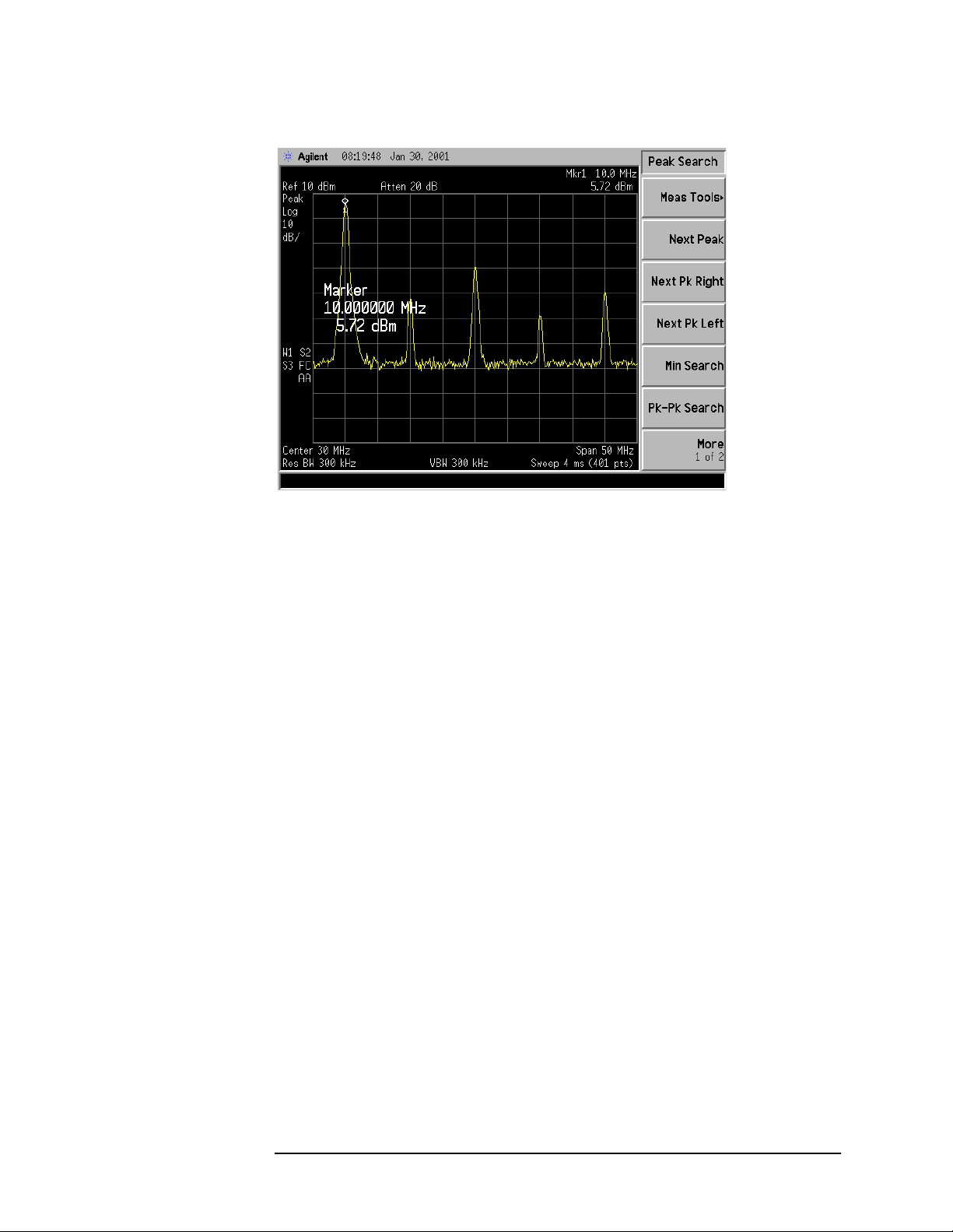
Figure 1-1 Placing a Marker on the 10 MHz Signal

Making Basic Measurements

Comparing Signals

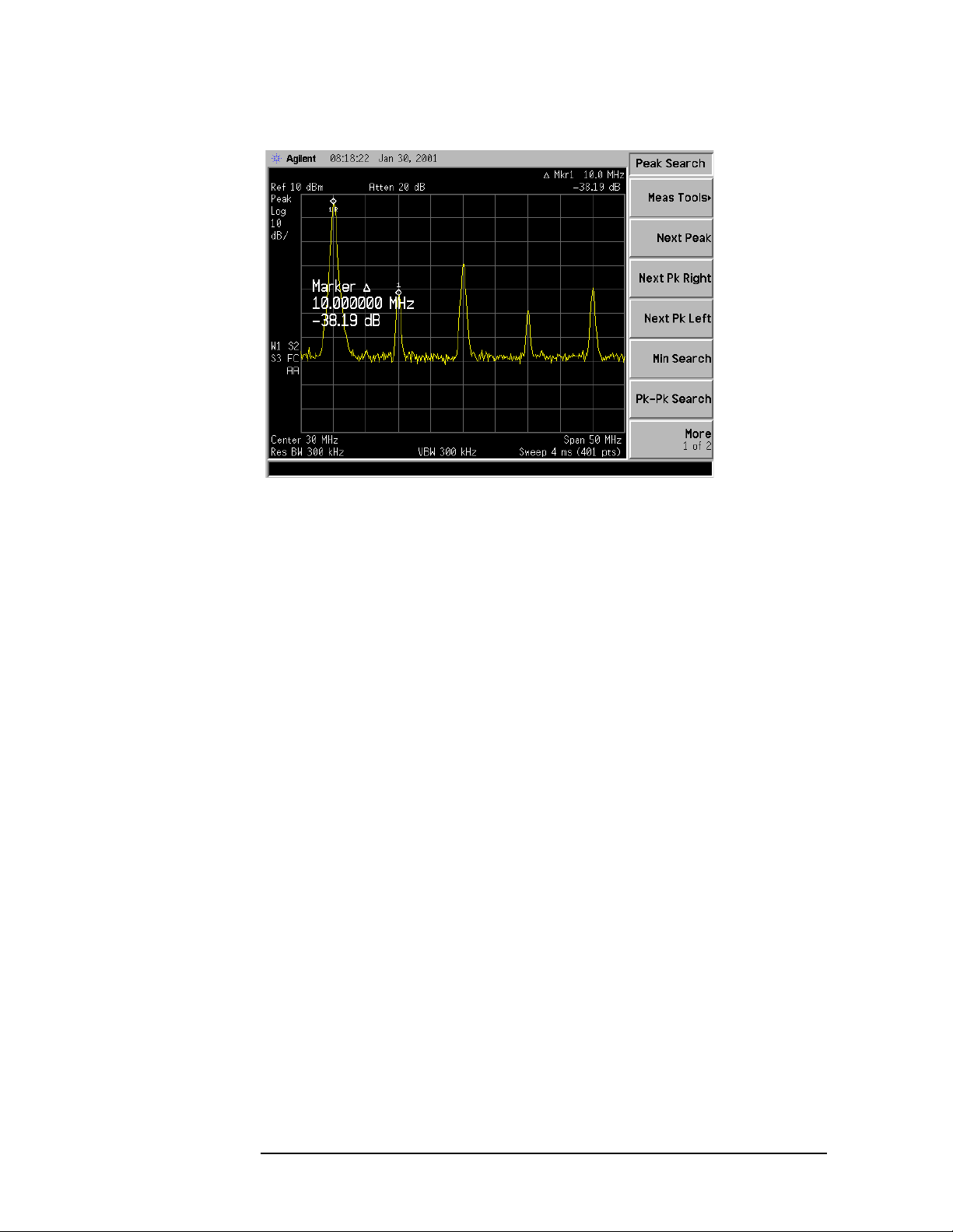
9. Press Marker, Delta, to activate a second marker at the position of the

first mark e r.

10.Move the second marker to another signal peak using the

front-panel knob, or by pressing

Next Pk Right or Next Pk Left. Next peak right is shown in Figure 1-2.

Peak Search and then either

The amplitude and frequency difference between the markers is
displayed in the ac tive function block and in the upp er right corner
of the screen. See Figure 1-2.

11. The resolution of the ma rker readings can be increased by turning

on the frequency count function. For more information refer to

“Making Better Frequency Measurements” on page 22.

12.Press Marker, Off to turn the markers off.

Chapter 1 11

Making Basic Measurements

Comparing Signals

Figure 1-2 Using the Marker Delta Function

Signal Comparison Example 2:

Measure the frequency a nd amplitude difference between two signa ls
that do not appear on the screen at one time. (This technique is useful
for harmonic distorti on tes ts when narrow span a nd narrow ba ndwi dth
are necessary to measure the lo w level ha rmonics.)

1. Perform a factory preset by pressing Preset, Factory Preset (if

present).

2. Connect the 10 MHz REF OUT from the rear panel to the

front- panel INPUT.

3. Set the center freq uency to 10 MHz by pressing FREQUENCY,

Center Freq, 10, MHz.

4. Set the span to 5 MHz by pressing SPAN, 5, MHz.

5. Set the resolution band width to spectrum analyzer coupling by

pressing BW/Avg, Res BW (SA).

6. Set the Y-Axis Units t o dB m by pres sing AMPLITUDE, More,

Y-Axis Units,

7. Set the reference level to 10 dBm by pressing AMPLITUDE, Ref Level,

10, dBm.

dBm.

The 10 MHz reference signal appears on the display.

8. Press Peak Search to place a marker on the peak.

9. Press Marker→, Mkr→CF Step to set the center frequency step size

equal to the frequency of the fundamental signal.

12 Chap ter 1

Making Basic Measurements

Comparing Signals

10.Press Marker, Delta to anchor the position of the first marker and

activate a second marker.

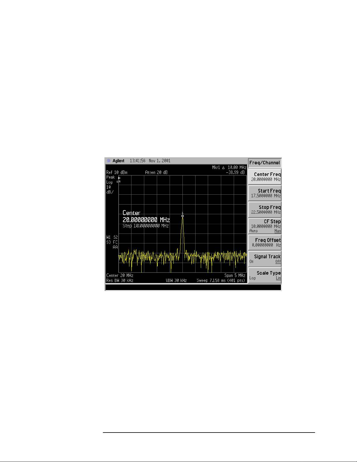
11. Press FREQUENCY, Center Freq, and the (↑) key to increase the center

frequency by 10 MHz. The first marker moves to the left edge of the
screen, at the a mplitude of the first signal peak. See Figure 1-3.

12.Press Peak Search to place the second marker on the highest signal

with the new center frequency setting. See Figure 1-3.
The annotation in the upper right corner of the screen indicates the

amplitude and frequency difference between the two markers.

13.To turn the markers o ff, press Marker, Off.

Figure 1-3 Frequency and Amplitude Difference Between Signals

Chapter 1 13

Making Basic Measurements

Resolving Signals of Equal Amplitude

Resolving Signals of Equal Amplitude

Two equal-amplitude input signals that are close in frequency can
appear as a single signal trace on the analyzer display. Responding to a
single-frequency signal, a swept-tuned analyzer tra ces out the shape of
the selected internal IF (intermediate frequency) filter. As you change
the filter bandwidth, you change the width of the displayed response. If
a wide filter is used and two equal-amplitude input signa ls are close
enough in frequency, then the two signals will appear as one signal. If a
narrow enough filter is used, the two input sig nals can be disc riminated
and will appe ar as separate pe aks. Thus, signal re solution is
determined by the IF filters inside the analyzer.

The bandwidth of the IF filter tells us how close together equal
amplitude signals can be and still be distinguished from each other. The
resolution bandwid th function selects an IF filter setting for a
measurement. Typically, resolution bandwidth is defined as the 3 dB
bandwidth of the fi lter. However, resolution bandwidth may also be
defined as the 6 dB or impulse bandwidth of the filter.

Generally, to resol ve two signals of equal amplitude, the resolution
bandwidth must be less than or eq ual to the freq uency separat ion of the
two signals. If the bandwidth is equal to the separation and the video
bandwidth is less than the resolution bandwidth, a dip of
approximately 3 dB is seen between the peaks of the two equal signals,
and it is clear that more than one signal is present. See Figure 1-7.

In order to keep the analyzer measurement calibrated, sweep time is
automatically set to a val ue tha t is i nvers ely propor tion al to the squar e

of the resolut ion bandwidth (1/BW

2

for resolution bandwidths ≥ 1kHz).
So, if the resolution bandwidth is reduced by a factor of 10, the sweep
time is increased b y a factor of 100 when sweep time and bandwidth
settings are coupl ed. Sweep time is also a function of the type of
detection selected (peak detection is faster than sample or average
detection). For the shortest measurement times, use the widest
resolution bandwidth that stil l pe rm its discrimination of all desir e d
signals. Sweeptime is also a function of which Detector is in use, Peak
detector sweeps more quickly than Sample or Average detector. The
analyzer allows you to select from 10 Hz (or 1 Hz with Option 1D5) to
3 MHz resolution ban dwidths in a 1, 3, 10 se qu e n ce and sel e ct a 5 MHz
resolution bandwid th. In addition you can select the three CISPR
bandwidt h s (200 Hz, 9 kH z , an d 120 kHz) for max imum measu rement
flexibility.

14 Chap ter 1

Resolving Signals Example:

Resolve two signals of equal amplitude with a frequency separation of
100 kHz.

1. Connect two sources to the analyzer input as shown in Figure 1-4.

Figure 1-4 Setup for Obtaining Two Signals

Making Basic Measurements

Resolving Signals of Equal Amplitude

2. Set one source to 300 MHz. Set the frequency of the other source to

300.1 MHz. The amplitude o f bo t h signals sho u ld be approxim at e l y

−20 dBm at the output of the bridge.

3. Set the analyzer as follows:
a. Press Preset, Factory Preset (i f pre s e n t).

b. Set the Y-Axis Units t o dB m by pres sing AMPLITUDE, More,

Y-Axis Units,

c. Set the center freq uency to 300 MHz by pressing F REQUE NCY,

Center Freq, 300, MHz.

d. Set the span to 2 MHz by pressing SPAN, Span, 2, MHz.
e. Set the resolution bandwidth to 30 0 kHz by pressing BW/Avg,

Res BW, 300, kHz.

dBm.

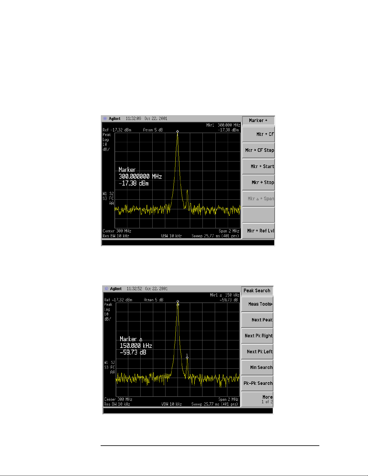
A single signal peak is visible. See Figure 1-5

NOTE If the signal peak is not present on the display, do the following:

1. Increase the span to 20 MHz by pressing SPAN, Span, 20, MHz.

The signal sho u ld b e v isi bl e .

2. Press Peak Search, FREQUENCY, Signal Track (On)

3. Press SPAN, 2, MHz to bring the signa l to center screen.

4. Press FREQUENCY , Signal Track (O ff)

Chapter 1 15

Making Basic Measurements

Resolving Signals of Equal Amplitude

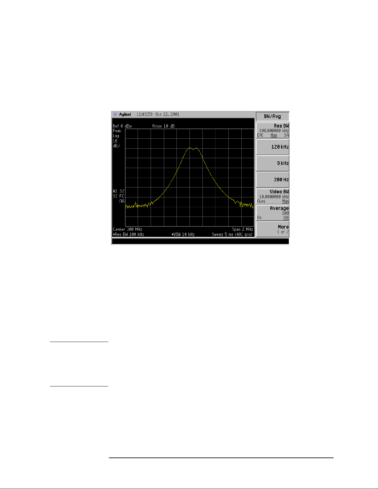
Figure 1-5 Unresolved Signals of Equal Amplitude

4. Since the resolution bandwidth must be less than or equal to the

frequency separation of the two signals, a resolution bandwi dth of
100 kHz must be used. Chan ge the resolution ban d width to 100 kHz
by pressing

BW/Avg, Res BW, 100, kHz. The peak of the si gnal has

become flattened indicating that two signals may be present as
shown in Figure 1-6. Use the knob or step keys to further reduce the
resolution bandwidth and b etter resolve the signals.

Figure 1-6 Resolving Signals of Equal Amplitude Before Reducing the

Video Bandwidth

16 Chap ter 1

Making Basic Measurements

Resolving Signals of Equal Amplitude

5. Decrease the video bandwidth to 10 kHz, by pressing Video BW, 10,

kHz. Two signals are now vis ibl e as sh o wn in Figure 1-7. Use the

front-panel knob or step keys to further reduce the resolution
bandwidth and better resolve the signals.

Figure 1-7 Resolving Signals of Equal Amplitude After Reducing the V ideo

Bandwidth

As the resolution bandw idth is decreased, resolution of the individual
signals is improved and the sweep time is increased. For fastest
measurement times, use the widest possible resolution bandwidth.
Under factory preset cond itions, the resolution bandwidth is “coupled”
(or linked) to the center frequency.

Since the resolution bandwidth has been changed from the coupled
value, a # mark appe ars next to Res BW in the lower-left corner of the
screen, indicating that the resolution bandwidth is uncoupled. (For
more information on coupling, refer to the Auto Couple key description
in the Agilent Technologies EMC Analyzers User’s Guide.)

NOTE T o resolve tw o signa ls of equal amplitud e with a frequency separat ion of

200 kHz, the resolution bandwidth m u st be less t han t h e signal
separation, and resolution of 100 kHz must be used. The next larger
filter, 300 kHz, would ex ceed the 200 kHz separation and would not
resolve the sign als.

Chapter 1 17

Making Basic Measurements

Resolving Small Signals Hi dden by Large Signals

Resolving Small Signals Hidde n by Lar ge
Signals

When dealing with the resolution of signals that are close together and
not equal in amplitud e, you must consider the shape of the IF filter of
the analy ze r, as well as its 3 dB bandwidth. (See “Resolving Signals of

Equal Amplitude” on page 14 for more information.) The shape of a

filter is defined by the selectivity, which is the ratio of the 60 dB
bandwidth to the 3 dB bandwidth. (Genera lly, the IF filters in this
analyzer have shape factors of 15:1 or less for resol ution bandwidths
≥1kHz and 5 :1 or less fo r reso lution band wi dt h s ≤ 300 Hz). If a small
signal is too close to a larger signal, the smaller signal can be hidden by
the skirt of the large r signal . To view the small er signal , you must s elect
a resolution bandwidth such that the separation between the two
signals (a) is greater than half the filter width of the larger signal (k)
measured at the amplitude level of the smaller signal. See Figure 1-8.

Figure 1-8 Resolution Bandwidth Requirements for Resolving Small

Signals

18 Chap ter 1

Resolving Small Sign als Hi dden by Large Signals

Resolving Signals Example:

Resolve two input signals w ith a frequency sep aration of 155 kHz and
an amplitude separation of 60 dB.

1. Connect two sources to the analyzer input as shown in Figure 1-9.

Figure 1-9 Setup for Obtaining Two Signals

Making Basic Measurements

2. Set one source to 300 MHz at −10 dBm.

3. Set the s e co n d so u rce t o 300.155 MHz, so that t h e s ig n al is 155 kHz

higher than the fi rst signal. Set the amplitude of the signal to

−70 dBm (60 dB below the first signal).

4. Set the analyzer as follows:
a. Press Preset, Factory Preset (i f pre s e n t).

b. Set the Y-Axis Units t o dB m by pres sing AMPLITUDE, More,

Y-Axis Units,

c. Set the center freq uency to 300 MHz by pressing F REQUE NCY,

Center Freq, 300, MHz.

d. Set the span to 2 MHz by pressing SPAN, Span, 2, MHz.

NOTE If the signal peak is not present on the display, do the following:

1. Increase the span to 20 MHz by pressing SPAN, Span, 20, MHz.

dBm.

The signal should now be visible.

2. Press Peak Search, FREQUENCY, Signal Track (On)

3. Press SPAN, 2, MHz to bring the signa l to center screen.

4. Press FREQUENCY , Signal Track (O ff)

e. Set the resolution bandwidth to spec trum analyzer coupling by

pressing BW/Avg, Resolution BW (SA).

Chapter 1 19

Making Basic Measurements

Resolving Small Signals Hi dden by Large Signals

5. Set the 300 MHz signal to the reference level by pressing Mkr → and

Mkr → Ref Lvl.

then
If a 10 kHz filter with a typical shape f actor of 1 5:1 i s us ed, the filter

will have a bandwidth o f 150 kHz at the 60 dB poin t . Th e
half-bandwidth (75 kHz) is narrower than the frequency separation,
so the input sig nals will be resolv ed . See Figure 1-10.

Figure 1-10 Signal Resolution with a 10 kHz Resolution Bandwidth

6. Place a marker on the smaller signal by pressing Marker, Delta,
Peak Search, Next Pk Right. Refer to Figure 1-11.

Figure 1-11 Signal Resolution with a 10 kHz Resolution Bandwidth

20 Chap ter 1

Making Basic Measurements

Resolving Small Sign als Hi dden by Large Signals

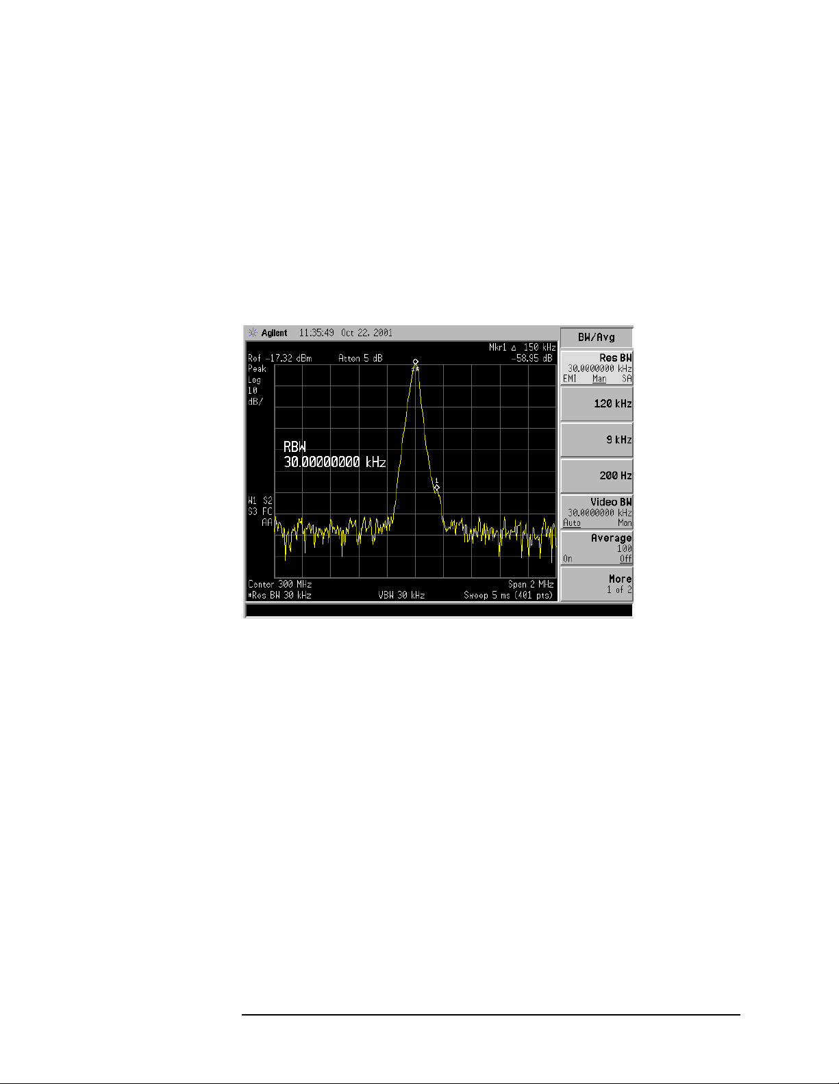
7. Set the resolution bandwidth to 30 kHz by pressing BW/Avg, Res BW,

30,

kHz.

When a 30 kHz filter is used, the 60 dB bandwidth could be as w ide
as 450 kHz. Since the half-bandwidth (225 kHz) is wider than the
frequency separation, the sig n als most likely wi ll no t be re solv e d.
See Figure 1-12. (In this example, we used the 60 dB bandwidth
value. To determine resolution capability for intermediate values of
amplitude level dif ferences, assume the filter ski rts between the
3 dB an d 60 dB po ints are ap proximately st raight.)

Figure 1-12 Signal Resolution with a 30 kHz Resolution Bandwidth

Chapter 1 21

Making Basic Measurements

Making Better Frequency Measurements

Making Better Fr equency Measurements

A built-in frequency co u n ter increas e s the re so lution and accuracy of
the frequency readout. W hen using this function, if the ratio of the
resolutio n ban dwidth to the span is too small (less than 0. 002), the
Marker Co unt: Wide n Res BW message appears on t h e displ ay. It
indicates that the resolution bandwidth is too narrow.

Better Frequency Measurement Example:

Increase the resolution and accuracy of the frequency read out on the
signal of intere st .

1. Perform a factory preset by pressing Preset, Factory Preset (if

present).

2. Turn on the internal 50 MHz amplitude reference signal of the

analyzer as follows:

• For the E7401A, use the inter nal 50 MHz amplitude reference

signal of the an alyzer as t h e signal bein g measur e d. P re ss

Input/Output, Amptd Ref (On).

• For all other models connect a cable between the front-panel

AMPTD REF OUT to the analyzer IN PUT, then press

Input/Output, Amptd Ref Out (On).

3. Set the center freq uency to 50 MHz by pressing FREQUENCY,

Center Freq, 50, MHz.

4. Set the span to 80 MHz by pressing SPAN, Span, 80, MHz.

5. Set the Y-Axis Units t o dB m by pres sing AMPLITUDE, More,

Y-Axis Units,

6. Set the resolution bandwidth to spectrum analyz er coupling pressing

BW/Avg, Resolution BW (SA).

7. Press Freq Count. (Note that Marker C oun t has On und erlined tur ning

dBm.

the frequency counter on.) The frequency and amplitude of the
marker and the word Marker will appear in th e active fun ct io n area
(this is not the counted result). The counted result appea rs in the
upper-right corner of the display.

8. Move the marker, with the front-panel knob, half-way down the ski rt

of the signal response. Notice that the readout in the ac tive
frequency function changes while the counted frequency result
(upper-right corner of display) does not. See Figure 1-13. To get an
accurate count, you do not need to place the marker at the exact
peak of the signal response.

22 Chap ter 1

Making Basic Measurements

Making Better Frequency Measurements

NOTE Marker count properly functions onl y on CW signals or discr ete spectr al

components. The marker mus t be >2 6 dB above the noise.

9. Increase the counter resolution by pressing Resolution and the n

entering the desired resolution using the step keys or the numbers
keypad. For example, press 10, Hz. The marker c ounter r ea dout is i n
the upper-right corner of the screen. The resolution can be set from
1Hz to 100kHz.

10.The marker counter remains on until turned off. Turn off the marker

counter by pressing

Freq Cou nt, then Marker Co unt (Off). Marker, Off

also turns the marker counter off.

Figure 1- 13 Using Marker Counter

Chapter 1 23

Making Basic Measurements

Decreasing the Frequency Span Around the Signal

Decreasing the Freq uency Span A round the
Signal

Using the analyzer signal track function, you can quickly decrease the
span while keeping the signal at center frequency. This is a fast way to
take a closer look at the area around the signal to identify signals that
would otherwise not be resolved.

Decreasing the Frequency Span Example:

Examin e a signal in a 200 kHz span.

1. Perform a factory preset by pressing Preset, Factory Preset (if

present).

2. Turn on the internal 50 MHz amplitude reference signal of the

analyzer as follows:

• For the E7401A, use the inter nal 50 MHz amplitude reference

signal of the an alyzer as t h e signal bein g measur e d. P re ss

Input/Output, Amptd Ref (On).

• For all other models connect a cable between the front-panel

AMPTD REF OUT to the analyzer IN PUT, then press

Input/Output, Amptd Ref Out (On).

3. Set the start fr equency to 20 MHz by pressing FREQUENCY,

Start Freq, 20, MHz.

4. Set the stop frequency to 1 GHz by pressing FREQUENCY, Stop Freq,

1, GHz.

5. Set the Y-Axis Units t o dB m by pres sing AMPLITUDE, More,

Y-Axis Units,

6. Set the resolution bandwidth to spectrum analyz er coupling pressing

BW/Avg, Resolution BW (SA).

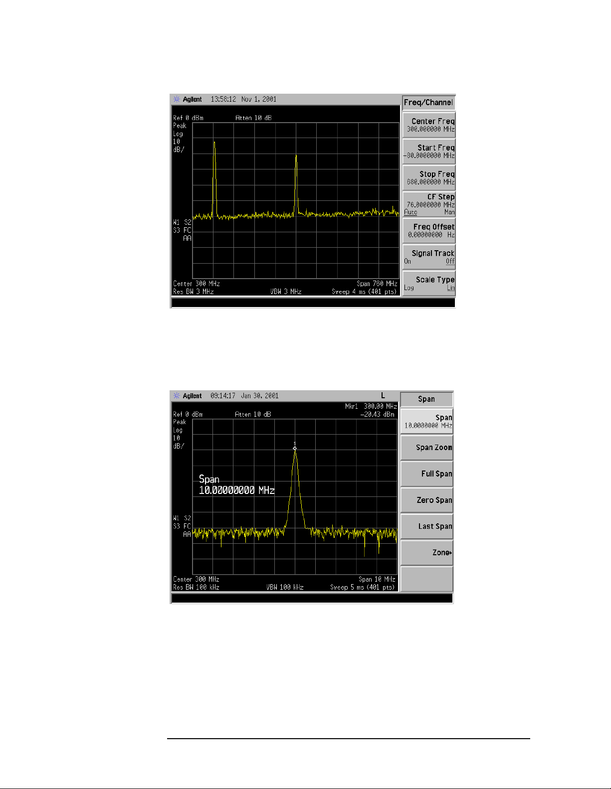
7. Press Peak Search to place a marker at the peak. See Figure 1-14.

dBm.

24 Chap ter 1

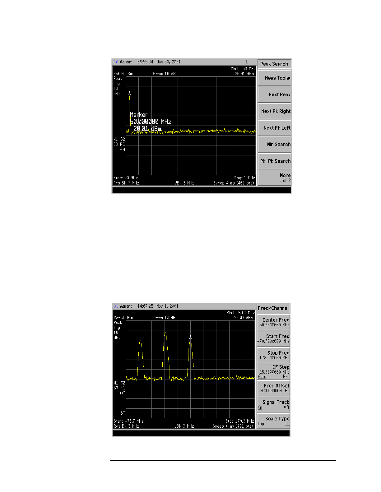
Figure 1-14 Detected Signal

Making Basic Measurements

Decreasing the Frequency Span Around the Signal

8. Turn on the frequency tracking function by press FREQ UENC Y an d

Signal Track and the signal w ill move to the center of the scr een, if it

is not already positioned there. See figure Figure 1-15. (Note that
the marker must be on the signal before turning signal track on.)

Because the signal track function automatically maintains the
signal at the center of the screen, you can reduce the span qui ckly for
a closer look. If the signal drifts off of the screen as you decrease the
span, use a wider f requency span. (You can also use
the

SPAN men u , as a qu i ck way to perfo rm the Peak Search,

FREQUENCY, Signal Track, SPAN key sequence.)

Figure 1-15 Signal with Signal Tracking On

Span Zoom, in

Chapter 1 25

Making Basic Measurements

Decreasing the Frequency Span Around the Signal

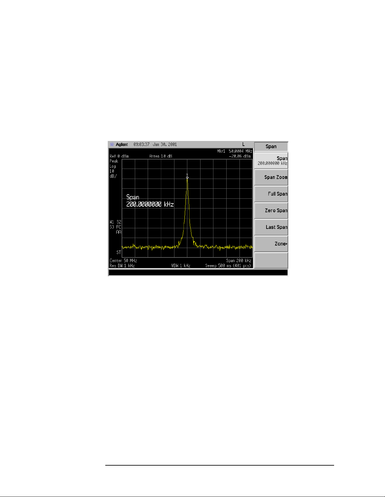
9. Reduce span and resolution bandwidth to zoom in on the marked

signal by pressing

SPAN, Span, 200, kHz.

If the span change is large enough, span will decrease in steps as
automatic zoom is completed. See Figure 1-16. You can also use the
front-panel knob or step keys to decrease the span and resolution
bandwidth values.

10.Press FREQUENCY , Signal Track (so that Off is underlined) to turn off

the signal track function.

Figure 1-16 After Zooming In on the Signal

26 Chap ter 1

Making Basic Measurements

T r acking Drifting Signals

T racking Drifting Signals

The signal track function is useful for tracking drifting sig nals that
drift relatively slowly. To place a marker on the signal you wish to
track, use
bring that signal to the center freq uency of the gratic ule a nd adjus t the
center frequency every sweep to bring the selected signal back to the
center. A quick way to perform the Peak Search, FREQUENCY,

Signal Track, SPAN key sequence is to use the Span Zoom key in the
SPAN menu.

Note that the primary functi on of the signal track function i s to track
unstable signals, not to track a signal as the center frequency of the
analyzer is changed. If you choose to use the signal track function when
changing center frequency, check to e nsure that the s i gnal f ound by the
tracking function is the correct signal.

T racking Signal Drift Example 1:

Peak Search. Pressing FREQUENCY, Signal Track (On) will

Use the signal track function to keep a drifting signal at the center of
the display and monitor its change.

This example requires a s ignal generator. The frequency of the signal
generator will be changed while you view the signal on the display of
the analyzer.

1. Conn e ct a signal gen e rat o r t o the an alyzer in put.

2. Set the signal generator frequency to 300 MHz with an amplitude of

−20 dBm.

3. Set the analyzer as follows:
a. Press Preset, Factory Preset (i f pre s e n t).

b. Set the Y-Axis Units t o dB m by pres sing AMPLITUDE, More,

Y-Axis Units,

c. Set the resolution bandwidth to the spectrum analyzer coupling

dBm.

by pressing BW/Avg, Resolution BW (SA). See Figure 1-17.

d. Set the center frequency to 300 MHz by pressing FREQUENCY,

Center Freq, 300, MHz.

Chapter 1 27

Making Basic Measurements

T r acking Drifting Signals

Figure 1-17 Signal With Default Span

4. Press Peak Search .

5. Set the span to 10 MHz by pressing SPAN, Span, 10, MHz.

See Figure 1-18.

Figure 1-18 Signal With 10 MHz Span

6. Press SPAN, Span Zoom, 500, kHz.

Notice that the sig nal has been held in the center of the display.
See Figure 1-19.

28 Chap ter 1

Figure 1-19 Signal With 500 kHz Span

7. Tune the frequency of the signal generator in 10 kHz increments.

Notice that the center frequency of the analyzer also c hanges in
10 kHz increments, centering the signal with each increment.
See Figure 1-20. Note that the center frequency has cha nged.

Making Basic Measurements

T r acking Drifting Signals

Figure 1-20 Using Span Zoom to Track a Drifting Signal

Chapter 1 29

Making Basic Measurements

T r acking Drifting Signals

8. The signal frequency dri ft can be read from the screen if both the

signal track and marker delta functions are active. Set the analyzer
and signal generator as follows:

a. Press Mar ker, Delta.
b. Tune the frequency of the signal generator. The marker readout

indicates the change in frequency and amplitude as the signal
drifts. See Figure 1-21.

Figure 1-21 Using Signal Tracking to Track a Drifting Signal

Tracking Signal Drift Example 2:

The analyzer can measur e the short- and long-term stability of a
source. The maximum amplitud e level and the frequency drift of an
input signal tr ace can be d isplaye d and he ld by using th e
maximum-hold function. You can also use the maximum hold func tion if
you want to determine how much of the frequency spectrum a signal
occupies.

1. Connect a signal generator to the analyzer input.

2. Set the signal generator frequency to 300 MHz with an amplitude of

−20 dBm.

3. Set the analyzer as follows:
a. Press Preset, Factory Preset (if present).

b. Set the Y-Axis Units to dBm by pressing AMPLITUDE, More,

Y-Axis Units,

c. Set the r esolution bandwidth to spectrum analyzer coupling by

pressing BW/Avg, Resolution BW (SA).

30 Chap ter 1

dBm.

d. Set the center frequency to 300 MHz by pressing FREQUENCY,

Center Freq, 300, MHz. See Figure 1-22.

Figure 1-22 Signal With Default Span

Making Basic Measurements

T r acking Drifting Signals

4. Press Peak Search.

5. Set the span to 10 MHz by pressing SPAN, Span, 10, MHz.

See Figure 1-23.

Figure 1-23 Signal With 10 MHz Span

Chapter 1 31

Making Basic Measurements

T r acking Drifting Signals

6. Press SPAN, Span Zoom, 500, kHz.

Notice that the sig nal has been held in the center of the display.
See Figure 1-24.

Figure 1-24 Signal With 500 KHz Span

7. Turn off the signal track function by pressing FREQUENCY,

Signal Track (Off).

8. To measure the excursion of the s ignal, press Trace/View, Max Hold.

As the signal varies, maximum hold maintains the maximum
responses of the inp ut signal.

Annotation on the left side of the screen indicates the trace mode.
For example, M1 S2 S3 indicates trace 1 is in maximum-hold mode,
trace 2 and trace 3 are in store-blank mode.

9. Press Trace/View, Trace, to select trace 2. (Trace 2 is selected when 2

is underlined.)

10.Press Clear Write to place trace 2 in clear-write mode, which displays

the current measurement results as it sweeps. Trace 1 remains in
maximum hold mode, showing the frequency shift of the signal.

11. Slowly change the fr equency of the signal generator ± 50 kH z in

1 kHz i ncrements. Your analyzer display should l ook similar to

Figure 1-25.

32 Chap ter 1

Making Basic Measurements

T r acking Drifting Signals

Figure 1-25 Viewing a Drifting Signal With Max Hold and Clear Write

Chapter 1 33

Making Basic Measurements

Measuring Low Level Signals

Measuring Low Level Signals

The ability of the analyzer to meas ure low level sig nals is limited by the
noise generated inside the analyzer. A signal may be masked by the
noise floor so that it is not visible. This sensitivity to low level signals is
affected by the mea surement setup.

The analyzer input attenuator and bandwidth settings affect the
sensitivity by changing the signal -to -nois e rati o. The attenua tor affects
the level of a signal passing through the instrument, wher eas the
bandw idt h affects the le vel of int e rn al noise withou t a ffe ct in g the
signal. In the first two examples in this section, the attenuator and
bandwidth se t tin gs are adj u st ed t o view lo w l eve l si gnals.

If, after adj usting the attenuation and resolution bandwidth, a signal is
still near the noise, visibility can be improved b y using the video
bandwidth and video averagi ng func ti ons , a s demonstrated i n the third
and fourth e x amples.

Measuring Low Level Signals Example 1:

If a signal is very close to the noise floor, reducing input attenuation
brings the signal out of the noise. Reducing the attenuation to 0 d B
maximizes signal power in the analyzer.

CAUTION The total po wer of all in pu t signals at th e a n alyzer inp u t m u st no t

exceed the maximum power lev el for the analyzer.

1. Connect a signal generator to the analyzer input.

2. Set the signal generator frequency to 300 MHz with an amplitude of

−80 dBm.

3. On the analyze, perform a factory preset by pressing Preset,

Factory Preset (if present).

4. Set the center freq uency of the analyzer to 300 MHz by pressing

FREQUENCY, Cent er Freq, 300, MHz.

5. Set the span to 5 MHz by pressing SPAN, Span, 5, MHz.

6. Set the resolution band width to spectrum analyzer coupling by

pressing

7. Set the Y-Axis Units t o dB m by pres sing AMPLITUDE, More,

Y-Axis Units,

BW/Avg, Res BW (SA) .

dBm.

8. Set the reference level to −40 dBm by pressing AMPLITUDE, Ref Level,

–40,

dBm.

9. Place the signal at center frequency by pressing Peak Search,

Marker→, Mkr→CF.

34 Chap ter 1

10.Reduce the span to 1 MHz. Press SPAN, Span, and then use the

step-down key (↓) until the span is set to 1 MHz. See Figure 1-26.

Figure 1-26 Low-Level Signal

Making Basic Measurements

Measuring Low Level Signals

11. Press AMPL ITUDE, Attenuation. Pre ss the ste p-u p key (↑) to select

20 dB attenuation. Increasing the attenuation moves the noise floor
closer to the s ignal.

A # mark appea rs next to the Atten annotation at the top of the
displa y, indicating t h e attenuation is n o longer couple d to other
analyzer settings.

Figure 1-27 Using 20 dB Attenuation

Chapter 1 35

Making Basic Measurements

Measuring Low Level Signals

12.To see the signal mo re cle arly, ent e r 0 dB. Ze ro de cibels of

attenuation makes the signal more visible. See Figure 1-28.

Figure 1-28 Using 0 dB Attenuation

CAUTION Before connecting other signals to the analyzer input, increase the RF

attenuation to protec t the a nalyzer inp ut: press

Attenuation so that Auto

is underlined or press Auto Couple.

Measuring Low Level Signals Example 2:

The resolution bandwidth can be decreased to view low level s ignals.

1. Connect a signal generator to the analyzer input.

2. Set the signal generator frequency to 300 MHz with an amplitude of

−80 dBm.

3. On the analyzer, perform a factory pr eset by pressing Preset,

Factory Preset (if present).

4. Set the center freq uency of the analyzer to 300 MHz by pressing

FREQUENCY, Cent er Freq, 300, MHz.

5. Set the span to 5 MHz by pressing SPAN, Span, 5, MHz.

6. Set the resolution band width to spectrum analyzer coupling by

pressing

7. Set the Y-Axis Units t o dB m by pres sing AMPLITUDE, More,

Y-Axis Units,

BW/Avg, Res BW (SA) .

dBm.

8. Set the reference level to −40 dBm by pressing AMPLITUDE, Ref Level,

–40, dBm.

36 Chap ter 1

9. Place the signal at center frequency by pressing Peak Search,

Marker→, Mkr→CF.

10.Press BW/Avg, Res BW, a nd then ↓. The low level s ig nal appears

more clearly because the noise level is reduced. As s hown in

Figure 1-29.

A # mark appea rs next to the Res BW annotation at the lower left
corner of the s creen, indicating that the resolution bandwidth is
uncoupled. As the resolution bandwidth is reduced, the sweep time
is increased to maintain calibrat ed data.

Figure 1-29 Decreasing Resolution Bandwidth

Making Basic Measurements

Measuring Low Level Signals

Measuring Low Level Signals Example 3:

Narrowing the video filter can be useful for noise measurements and
observation of low l evel signals close to the noise floor. T he video filter
is a post-detection low-pass filter that smooths the disp layed trace.
When signal responses near the noise level of the analyzer are visually
masked by the noise, the video filter can be narrowed to sm ooth this
noise and improve the visibility of the signal. (Reducing video
bandwidths requires slower sweep times to keep the analyzer
calibrated.)

Using the video bandwidth function, measure the amplitude of a low
level signal.

1. Conn e ct a signal gen e rat o r t o the an alyzer in put.

2. Set the signal generator frequency to 300 MHz with an amplitude of

−80 dBm.

Chapter 1 37

Making Basic Measurements

Measuring Low Level Signals

3. On the analyzer, perform a factory pr eset by pressing Preset,

Factory Preset (if present).

4. Set the center freq uency of the analyzer to 300 MHz by pressing

FREQUENCY, Cent er Freq, 300, MHz.

5. Set the span to 5 MHz by pressing SPAN, Span, 5, MHz.

6. Set the resolution band width to spectrum analyzer coupling by

pressing

7. Set the Y-Axis Units t o dB m by pres sing AMPLITUDE, More,

Y-Axis Units,

8. Set the reference level to −40 dBm by pressing AMPLITUDE, Ref Level,

–40,

9. Place the signal at center frequency by pressing Peak Search,

Marker→, Mkr→CF. See Figure 1-30.

BW/Avg, Res BW (SA) .

dBm.

dBm.

Figure 1-30 30 kHz Video Bandwidth

10.Narrow the video bandwidth by pressi ng BW/Avg, Video B W , and the

step-down key (↓). This clarifies the signal by smoothing the noise,
which allows better measurement of the signal amplitude.

A # mark appears next to the VBW annotation at the bottom of the
screen, indicating that the video bandwidth is not coupled to the
resolution bandwidth. See Figure 1-31. As the video bandwidth is
reduced, the sweep time i s increased to maintain calibrated da ta.

Instrument preset conditions couple the video bandwidth to the
resolution bandwidth. If the bandwidths are uncoupled when video
bandwidth is the active function, pressing

Video B W (so that Auto is

underlined) recouples the bandwidths.

38 Chap ter 1

Making Basic Measurements

Measuring Low Level Signals

NOTE The video bandwidth must be set wider than the resolution bandwidth

when measuring impulse noise levels.

Figure 1-31 Decreasing Video Bandwidth

Measuring Low Level Signals Example 4:

If a signal level is very close to the noise floor, video averaging is
another way to make the signal more visible.

NOTE The time required to construct a full trace that is averag ed to the

desired degree is approximately the same when using either the video
bandwidth or the video a veraging technique. The video bandwidth
technique completes the a veraging as a slow sweep is taken, whereas
the video averaging technique takes many sweeps to complete the
average. Characteristics of the signal being measured, such as drift and
duty cycle, determine whi ch technique is appropriate.

Video averaging is a digital process in which each trace po int is
averaged with the previous trace-point average. Sel ecting

Video Avg and Average (On) ch an g e s the de t e ct ion m o de fro m pe ak t o

sample. The result is a sudden drop in the displayed noise level. The
sample mode displays the instantaneous value of the signal at the end
of the time or freq uency interval represented by each display point,
rather than the value of the peak during the interval. Sample mode is
not used to measure si gnal amplitudes accurately because it may not
find the true peak of the signal.

Average Type,

Video aver aging cla rifies low-leve l signals in wide ba n d widths by
averaging the signal and the noise. As the analyzer takes sweeps, you
can watch video averaging smooth the trace.

Chapter 1 39

Making Basic Measurements

Measuring Low Level Signals

1. Connect a signal generator to the analyzer input.

2. Set the signal generator frequency to 300 MHz with an amplitude of

−80 dBm.

3. On the analyzer, perform a factory pr eset by pressing Preset,

Factory Preset (if present).

4. Set the center freq uency of the analyzer to 300 MHz by pressing

FREQUENCY, Cent er Freq, 300, MHz.

5. Set the span to 5 MHz by pressing SPAN, Span, 5, MHz.

6. Set the resolution band width to spectrum analyzer coupling by

pressing

7. Set the Y-Axis Units t o dB m by pres sing AMPLITUDE, More,

Y-Axis Units,

8. Set the reference level to −40 dBm by pressing AMPLITUDE, Ref Level,

BW/Avg, Res BW (SA) .

dBm.

–40, dBm.

9. Place the signal at center frequency by pressing Peak Search,

Marker→, Mkr→CF. See Figure 1-32.

Figure 1-32 Without V ideo Averaging

10.Pressing BW/Avg, Average Type, (Video Avg), Average (On), in it iates

the video averaging r outine. As the averaging routine smooths the
trace, low level signals be come more visible. Av era ge 100 appears
in the active function block. The number represents the number of
samples (or sweeps) taken to complete the averaging routine. Once
the set number of sweeps has been completed, the analyzer
continues to provide a running average based on this set number.

40 Chap ter 1

11. T o set the number of samples, use the numeric keypad. For example,

press

Average (On), 25, Enter. As shown in Figure 1-33.

During averaging, the current sample number appears at the left
side of the gra ticule. The number of samples equals the number of
sweeps in the averaging routine. Changes in active function settings,
such as the center frequency or reference level, will restart the
sampling. The sampling will also restart if video averaging is turned
off and then on a gain. To see the sample number increment, turn
video aver aging off an d o n ag ain by pressin g

Average

(On).

Figure 1-33 Using the Video Averaging Function

Making Basic Measurements

Measuring Low Level Signals

Average (Off),

Chapter 1 41

Making Basic Measurements

Identifying Distortion Products

Identifying Distortion Products

Distortion from the Analyzer

High level input signals may cause analyzer distortion products that
could mask the real distortion measured on the input signal. Using
trace 2 and the RF attenuator , you can determine which signals, if any,
are internall y g e n erat e d di st o rt ion pro du c t s.

Identifying Analyzer Generated Distortion Example:

Using a si gnal from a signal gen erator, determin e wh e t h e r the
harmonic distortion products are generated by the analyzer.

1. Connect a signal generator to the analyzer INPUT.

2. Set the signal generator fr equency t o 200 MHz and the amplitude to

0dBm.

3. On the analyzer, perform a factory pr eset by pressing Preset,

Factory Preset (if pre se nt).

4. Set the Y-Axis Units t o dB m by pres sing AMPLITUDE, More,
Y-Axis Units,

5. Set the resolution band width to spectrum analyzer coupling by

pressing

6. Set the center freq uency of the analyzer to 400 MHz by pressing

FREQUENCY, Cent er Freq, 400, MHz.

7. Set the sp an to 5 00 MHz by press ing SPAN, Span, 500, MHz.

dBm.

BW/Avg, Res BW (SA) .

The signal produces har monic distortion products in the analy zer
input mix e r as shown in Figure 1-34.

42 Chap ter 1

Figure 1-34 Harmonic Distortion

8. Change the center frequency to the value of one of the observed

harmonics by pre ssing

Making Basic Measurements

Identifying Disto rtion Products

Peak Search, Next Peak, Marker→, Mkr→CF .

9. Change the span to 50 MHz: press SPAN, Span, 50, MHz.

10.E n sure t h at the signal is still at th e ce n t er frequ e n cy, if necessary

press Peak Search, Marker→, Mkr→CF.

11. Change the attenuation to 0 dB: press AMPLITUDE, Attenuation, 0,

dBm. Your display should be similar to Figure 1-35.

Figure 1-35 Harmonic Distortion with 0 dB Attenuation

Chapter 1 43

Making Basic Measurements

Identifying Distortion Products

12.To determine whether the harmonic distortion pr oducts are

generated by the analyzer, first sa ve the screen data in trace 2 as
follows:

a. Press Trace/View, Trace (2), then Clear Write.
b. Allow the trace to update (two sweeps) and press Trace/View , View,

Marker, Delta. The analyzer display sho ws the stor ed da ta in trac e

2 and the measured da ta in trace 1.

13.Next, increase the RF attenuation by 10 dB: press AMPLITUDE,

Attenuation, and the step-up key (↑) twice. See Figure 1-36.

Notice the ∆Mkr1 amplitude readi ng. This is the difference in the
distortion product amplitude reading s between 0 dB and 10 dB input
attenuation settings. If the ∆Mkr1 amplitude absolute va lu e is
approximately ≥1 dB for an input attenuator cha nge, the distortion
is being generated, at least in part, by the analyzer. In this case more
input attenuation is necessary.

Figure 1-36 RF Attenuation of 10 dB

14.Press P eak S earch , Marker, Delta

Change the attenuation to 15 dB by pressing Attenuation, 15, dB.
If the ∆Mkr 1 amplitude absolute value is approximately ≥1dB as

seen in Figure 1-36, then more input attenuation is requir ed; some
of the measured distortion is internally generated. If there is no
change in the signal level, the distortion is not gener ated internally.
For example, the signal that is causing the distortion shown in

Figure 1-37 is not high enough in amplitude to cause internal

distortion in the analyzer so any distortion that is dis played is
present on the input signal.

44 Chap ter 1

Figure 1-37 No Harmonic Distortion

Making Basic Measurements

Identifying Disto rtion Products

Third-Order Intermodulation Distortion

Two-tone, third-order intermodulation dis tortion is a common test in
communication systems. When two s ignals are present in a non-linear
system , th e y ca n in t e ract and crea t e th ird-orde r in t e rmodulat io n
distortion products that are located close to the origi nal signals. These
distortion products ar e generated by system components such as
amplif iers and mixe rs .

Identifying TOI Distortion Example:

Test a device for third-order intermodulation. This example uses two
sources, one set to 300 MHz and the other to approximately 301 MHz.
(Other source frequencies may be substituted, but try to mainta in a
frequency separation of approximately 1 MHz.)

1. Connect the equipment as shown i n Figure 1-38. This combination of

signal generators, low pass filters, and directional coupler (used as a
combiner) results in a two-tone source with very low
intermodulation dis tortion. Although the distortion from this setup
may be better than the specified performance of the analyzer, it is
useful for determining the TOI performance of the source/analyzer
combination. After the performance of the source/analyzer
combination has been verified, the device-under-test (D UT ) (for
example, an amplifier ) would be inserted between the directional
coupler output and the analyzer input and another measurement
would be ma de .

Chapter 1 45

Making Basic Measurements

Identifying Distortion Products

Figure 1-38 Third-Order Intermodulation Equipment Setup

NOTE The combiner should have a high degree of isolation between the two

input ports so th e sources do not inter mo du l at e .

2. Set one source (signal generator) to 300 MHz and the other source to

301 MHz, for a frequency separation of 1 MHz. Set the s our c es eq ual
in amplitude as measured by the analyzer (in thi s example, they a r e
set to −5dBm).

3. On the analyzer, perform a factory pr eset by pressing Preset,

Factory Preset (if pre se nt).

4. Set the Y-Axis Units t o dB m by pres sing AMPLITUDE, More,
Y-Axis Units,

5. Set the resolution band width to spectrum analyzer coupling by

dBm.

pressing BW/Avg, Res BW (SA).

6. Set the span to 5 MHz by pressing SPAN, Span, 5, MHz. This is wide

enough to include the distortion products on the screen.

7. Tune both test signals onto the screen by setting the center

frequency 300.5 MHz, press FREQUENCY, Center Freq, 300.5, MHz.
If necessary, use the front-panel knob to center the two test signals

on the display.

8. T o be sure the distortion pro ducts are resolv ed, reduce the resoluti on

bandwidth until the distortion products are visible by press ing

BW/Avg, Res BW, and then us e the step-down key (↓) to reduce the

resolution bandwidth until the distortion products are visible.

9. For best dynamic range, set the maximum mixer input level to

−30 dBm and move the signal to the reference level: press

AMPLITUDE, More, Max Mixer Lvl, –30, dBm.

46 Chap ter 1

The analyzer automatically sets the attenuation so that a signal at
the refe rence lev el will be a maximum of −30 dBm at the inpu t
mixer.

10.Press BW/Avg, Res BW, and the n use the step-down key (↓) to reduce

the resolution bandwidth until the distortion products ar e visible.

11. T o measure a dis tortion product , press Peak Search to plac e a ma rk er

on a source sign al .

12.Set the marked signal to the reference level by pressing Mkr → and

then

Mkr → Ref Lvl.

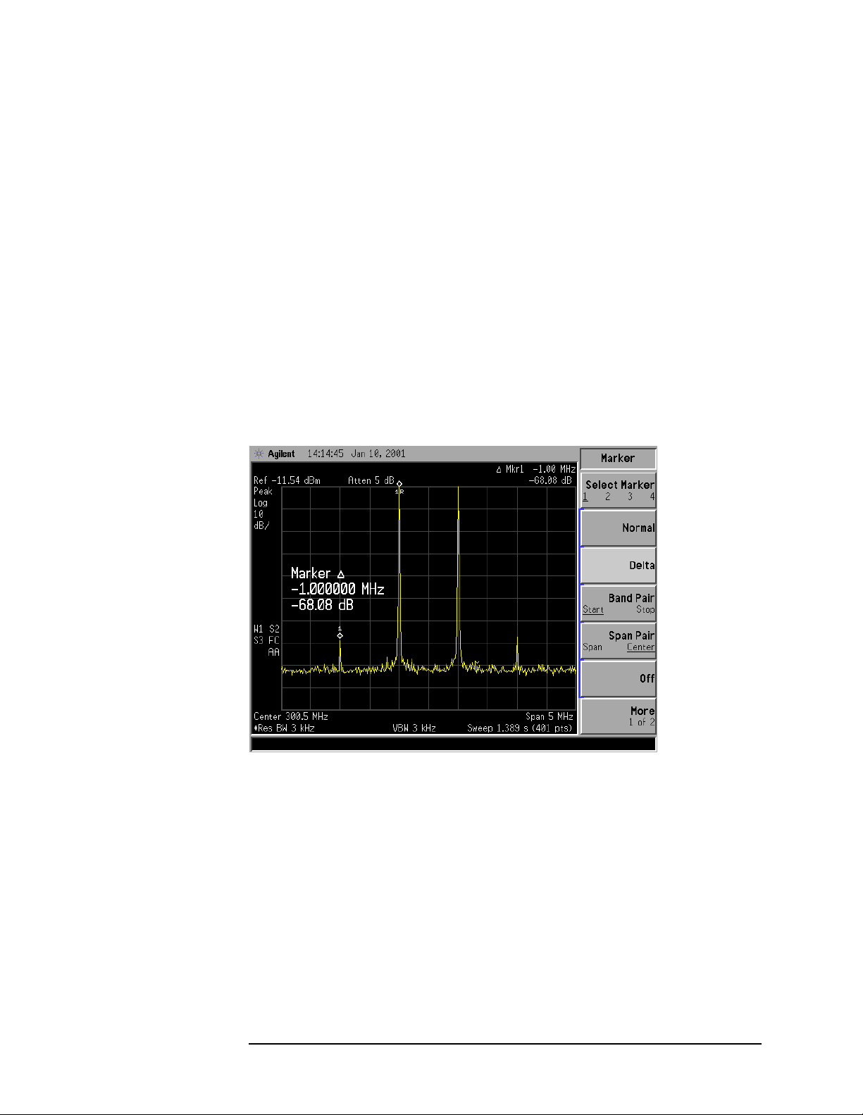
13.To activate the second marker, press Marker, Delta, Peak Search.

Using the

Next Peak key to place the second marker on the peak of

the distortion pr oduct that is beside the test signal. The difference
between the markers is displayed in the active function area. See

Figure 1-39.

Figure 1-39 Measuring the Distortion Product

Making Basic Measurements

Identifying Disto rtion Products

14.To measure the other distortion product, pres s Mar ker, Normal,

Peak Search, Next Peak. This places a marker on the next highest

peak, the other source signal.

15.To measure the difference between this test signal and the second

distortion product, press Delta, Peak Search. Using the Next Peak key
to place the second marker on the peak of the second distortion
product. See Figure 1-40.

Chapter 1 47

Making Basic Measurements

Identifying Distortion Products

Figure 1-40 Measuring the Distortion Product

48 Chap ter 1

Making Basic Measurements

Measuring Signal-to-Noise

Measuring Signal-to-Noise

The signal-to-noise mea surement procedure below may be adapted to
measure any signal in a system if the signal (carrier) is a discrete tone.
If the signal in your system is modulated, it will be necessary to modify
the procedure to correctly measure the modulated signal level

In this example the 50 MHz amplitude reference signal is used as the
fundamental source. The a mplitude reference signal is assumed to be
the signal of i nter es t a nd the internal noise of the anal yzer is m easur ed
as the system noise. To do this, you will need to set the input attenuat or
such that both the signal and the noise are well within the calibrated
region of the display.

Signal-to-Noise Measurement Example:

Perform the steps below to measure the signal-to-noise.

1. Perform a factory preset by pressing Pre set, Factory Preset (if

present).

2. Turn on the internal 50 MHz ampl it u de re fe rence signal of the

analyze r as fo l lo ws:

• For the E7401A, use the internal 50 MHz amplitude reference

signal of the analyzer as the signal being measured. Press

Input/Output, Amptd Ref ( On).

• For all other models connect a cable between the front-panel

AMPTD REF OUT to the analyzer INPUT, then press

Input/Output, Amptd Ref Ou t (On).

3. Set the center frequency to 50 MHz by pressing FREQUENCY,

Center Freq, 50, MHz.

4. Set the span to 1 MHz by pressing SPAN, Span, 1, MHz.

5. Set the Y-Axis Units to dBm by pressing AMPLITUDE, More,

Y-Axis Units,

6. Set the resolution bandwidth to spectrum analyzer coupling by

dBm.

pressing BW/Avg, Res BW (SA).

7. Set the reference level to –10 dBm by pressing AMPLITUDE, Ref Level,

–10,

dBm.

8. Set the attenuation to 40 dB by pressing AMPLITUDE, Attenuation, 40,
dB.

9. Press Peak Search to place a marker on the peak of the signal.

10.Press Marker, Delta, 200, kHz to put the delta marker in the noise at

the spe cified offse t , in th is case 200 kH z .

Chapter 1 49

Making Basic Measurements

Measuring Signal-to-Noise

11. Press More, Function, Marker Noise to view the res ults of the si gna l t o

noise measurement. See Figure1-41.

Figure 1-41 Measuring the Signal-to-Noise

Read the signal-to-noise in dB/Hz, that is with the noise value
determined for a 1 Hz noise bandwidth. If you wish the noise value for a
different bandwidth, decrease the ratio by . For example, if

10 log× BW()

the analyzer reading is −70 dB/Hz but you have a channel band width of
30 kHz:

S/N 70 dB/Hz– 10 30 kHz()log×+ 25.23 dB– 30 kHz()⁄==

Note that the display detection mode is now average. If the delta
marker is within half a division of the response to a discrete sig nal, the
amplitu de re fe re n ce signal in t h is case, ther e i s a po t e ntial for erro r in
the noise m easurement. See “Making Noise Measurements” on page 51.

50 Chap ter 1

Making Basic Measurements

Making Noise Measurements

Making Noise Measurements

There are a variety of ways to measure noise power. The first decision
you must make is whether you w a nt to measure noise power at a
specific frequency or the total power over a specified frequency range,
for example over a cha nnel bandwidth.

Noise Measurement Example 1:

Using the marker function, Marker Noise, is a simple method to make a
measurement at a single frequency. In this example, attention must be
made to the potential errors due to discrete signal (spectral
components). This measurement wil l be made near the 50 MHz
amplitude reference sig nal to illustrate the use of

1.

Perform a factory pr eset by pressing Preset, Factory Preset (if
present).

2. Turn on the internal 50 MHz ampl it u de re fe rence signal of the

analyze r as fo l lo ws:

Marker Noise.

• For the E7401A, use the internal 50 MHz amplitude reference

signal of the analyzer as the signal being measured. Press

Input/Output, Amptd Ref (On).

• For all other models connect a cable between the front-panel

AMPTD REF OUT to the analyzer INPUT, then press

Input/Output, Amptd Ref Ou t (O n ).

3. Set the center frequency to 49.98 MHz by pressing FREQUENCY,

Center Freq, 49.98, MHz.

4. Set the span to 100 kHz by pressing SPAN, Span, 100, kHz.

5. Set the resolution bandwidth to 1 kHz by pressing BW/Avg,

Res BW (Man), 1, kH z.

6. Set the Y-Axis Units to dBm by pressing AMPLITUDE, More,

Y-Axis Units,

7. Set the attenuation to 60 dB by pressing AMPLITUDE, Attenuation

(Man), 60, dB. See Figure 1-42.

NOTE When making noise measurements and AMPLITUDE, Scale Type (Log) is

dBm.

selected (10 dB/division), position the trace between 3 and 6 graticule
lines above the bottom by adjusting the reference level (AM PLITUDE,

Ref Level). Measurement inaccuracies may occur if d isplayed trace is

positioned outside this range.

Chapter 1 51

Making Basic Measurements

Making Noise Measurements

Figure 1-42 Setting the Attenuation

8. Activate the noise marker by pressing Marker, More, Function,

Marker Noise.

Note that the display d etection automatically changed to “Avg”
which can be manually set b y pressing Det/Demod,

Average (Video/RMS). The marker is floating between the maximum

and the minimum of the noise. For firmware revisions earlier than
A.08.00, the detecti on type when using
sample. If you wish to use sample detection, press

Detector, Sample and ver ify t ha t “Average Type” is set to “Video

Marker Noise cha n ge d to

Det/Demod,

average” by pre ssing BW /Avg, Average Type, Vid e o Avg. This is not
recommended as it is slower and does not increase accuracy.

The marker readout is in dBm(Hz) or dBm per unit bandwidth. See

Figure 1-43. For noise power in a different bandwidth, add

10 log× BW()
10 log 1000()×

. For exampl e , for n o ise po we r in a 1 kH z ban dwidth, ad d

or 30 dB to the noise marker value.

52 Chap ter 1

Figure 1-43 Activating the Noise M arker

9. The noise marker value is ba sed on the mean of 5% of the total

number of sweep points centered at the marker. The points averaged
span one-half of a division. To see the effect, move the marker to the
50 MHz signal by pr e ssing Marker, 50, MHz (or use the front-panel
knob to place marker at 50 MHz). See Figure 1-44.

Making Basic Measurements

Making Noise Measurements

Figure 1-44 Noise Marker at 50 MHz

10.The marker does not go to the peak of the signal because not all

averaged points are at the peak of the signal. Widen the resolution
bandwidth by pressing BW/Avg, Res BW, 10, kHz (or up arrow) to see
what happens. The marker is now much closer to the peak of the
signal. See Figure 1-45.

Chapter 1 53

Making Basic Measurements

Making Noise Measurements

NOTE Notice the video bandw idth changed to 100 kHz. The ratio between the

video bandwidth (VBW) and the resolution b andwidth (RBW) must be ≥
10/1 to maintain the accuracy of the measurement.

Figure 1-45 Increased Resolution Bandwidth

11. Return the resolution bandwidth to 1 kHz . Press BW/Avg, 1, kHz.

12. Measure the noise very close to the signal by pressing Marker,

50.0000, MHz (or use the front-panel knob to place the marker). See

Figure 1-46.

Note that the marker read s a value that is too high beca use some of
the averaged trace points are on the skirt of the signal response.

54 Chap ter 1

Figure 1-46 Noise Marker in Signal Skirt

13. Set the analyzer to zero span at the marker frequency by pressing

Mkr →, Mkr → CF, SPAN, Zero Sp an, Marker. Note that the marker

amplitude value is now correct since all points averaged are at the
same frequency and not influenced by the shape of the bandwidth
filter. See Figure 1-47.

Making Basic Measurements

Making Noise Measurements

Figure 1-47 Noise Marker with Zero Span

Chapter 1 55

Making Basic Measurements

Making Noise Measurements

Noise Measurement Example 2:

The Normal marker can also be used to make a single frequency
measurement as described in the previous example, again using video
filtering or averaging to obt ain a rea sonably stable measu rement .
While v id e o averagi ng automatical ly selects t h e sample display
detection mode, video filtering does not. With sufficient filtering that
results in a smooth trace, ther e is no dif ference between the sample and
peak modes because the filtering takes place before the signa l is
digitized.

Be sure to account for the fact that the averaged noise is displayed
approximately 2 dB too low for a nois e bandwidth equal to the
resolution bandwidth. T herefore, you must add 2 dB to the marker
reading. For example, if the marker indicates –100 dBm, the actua l
noise le vel is –98 dBm.

Noise Measurement Example 3:

You may use adjustable mark ers to set the frequency span over which
power is measure d. The m arkers al low you to e asily and co n venien t ly
select any arbitrary po rt io n o f t h e displayed sign al for measu re ment.
However , while the analyzer doe s select the average (vi deo/rms) display
detection mo de, you must se t a ll o f t h e othe r paramete rs.

1. Reset the analyzer by pressing Preset, Factory Preset (if present ).

2. Tune the analyzer to the frequency of 50 MHz. In this example we

are using the amplitude reference signal. Press

MHz.

3. Set the sp an to 1 00 kHz by press i ng SPAN, 100, kHz.

4. Set the Y-Axis Units t o dB m by pres sing AMPLITUDE, More,

Y-Axis Units,

5. Set the resolution b andwidth to 1 kHz by pressing BW/Avg,

Resolution BW, 1, kHz.

6. Set the reference level to −20 dBm by pressing AMPLITUDE, Ref Level,

dBm.

FREQUENCY, 50,

–20, dBm.

7. Set the input attenuator to 40 dB by pressing Atte nu ation, 40, dB.

8. Set the marker span to 40 kHz by pressing Marker, Span Pair (Span) ,

40, kHz.
The resolution bandwidth should be about 1 to 3% of the

measurement (marker) span, 40 kHz in this example. The 1 kHz
resolution bandwidth that the analyzer has chosen is fine. The vi deo
bandwidth should be ten times wider.

9. Set the video bandwidth to 10 kHz by pressing BW/Avg,

Video BW (Man), 10, kHz.

56 Chap ter 1

10.Measure the power between markers by pressing Marker, More,
Function, Band Power. The analyzer displays the total power between

the markers. See Figure 1-48.

11. Add a discrete tone to see the effects of the reading. Turn on the

internal 50 MHz amplitude reference signal of the analyzer (if you
have not already done so) as follows:

• For the E7401A, use the internal 50 MHz amplitude reference

signal of the analyzer as the signal being measured. Press

Input/Output, Amptd Ref (On).

• For all other models connect a cable between the front-panel

AMPTD REF OUT to the analyzer INPUT, then press

Input/Output, Amptd Ref Ou t (O n ).

Figure 1-48 Viewing Power Between Markers

Making Basic Measurements

Making Noise Measurements

12.Move the measured span by pressing Marker, Span Pair (Center).

Then use the knob to exclude the tone and note reading. You could
have also used

Band Pair or Delta Pair to set the measurement start

and stop points inde pen de n tly. See Figure 1-49.

Chapter 1 57

Making Basic Measurements

Making Noise Measurements

Figure 1-49 Measuring the Power in the Span

58 Chap ter 1

Making Basic Measurements

Demodulating AM Signals (Using the Analyzer As a Fixed T uned Receiver)

Demodulating AM Signals (Using the Analyzer
As a Fixed Tuned Receiver)

The zero span mode can be used to recover amplitude modulation on a
carrier signal. The an alyzer op e rat e s as a fixed-tu n e d receiver i n zer o
span to provide time d omain measurements.

Center frequency in the sw ept-tuned mode becomes the tuned
frequency in zero span. T he horizontal axis of the screen bec omes
calibrated in time only, rather than both frequency and time. Markers
display amplitude and time values.

The following functions establish a clear display of the wa veform:

• Trigg er s tabilizes the waveform trace on the displa y by tr iggering on

the modulation envelop e. If the modulation of the signal is stable,
video trigger sy nchronizes the sweep with the demodulated
waveform.

• Linear mode should be used in amp litude modulation (AM)

measurements to avoid d istortion caused by the logarithmic
amplifier whe n de modulating si gnals.

• Sweep time adjusts the full sweep time from 5 ms to 2000 s. (20 µs to

2000 s if Option A YX is installed). The sweep time readout refers to
the full 10-division graticule. Divide this value by 10 to determine
sweep time per di vi sio n.

• Resolution and video bandwidth are selected according to the signal

bandwidth.

Each o f the co u pled fun ct ion valu es remain s at its cu rre n t value whe n
zero span is act ivated. Video bandw idt h is co u pled to r e solution
bandwidth. Sweep time is not coupled to any other function.

NOTE Refer to “Dem o du la t ing and Listen ing to an AM Sig nal” on page 88 for

more in fo rmatio n on signal demo d u lation.
T o obtain an AM signal, you can either connect a source to the analyzer

input and set the so u rc e for amplitude mo du l at ion , or co n ne ct an
antenna to the analyzer input and tune to a commercial AM broadcast
station.

Demodulating an AM Signal Example 1:

View the modulation waveform of an AM signal in the tim e domain.

1. Conn e ct an R F sig n al source to the an alyzer INPU T. For this

example, an Agilent E4433B Signal Generator was used with the
following sett ings:

a. RF Frequency 300 MHz

Chapter 1 59

Making Basic Measurements

Demodulating AM Signals (Using the Analyzer As a Fixed Tuned Receiver)

b. RF Output Power –10 dBm
c. AM On
d. AM Rate 1 kHz
e. AM Dep th 80%

2. Set the analyzer as follows:
a. Press Preset, Factory Preset (if present).

b. Set the center frequency to 300 MHz by pressing FREQUENCY,

Center Freq, 300, MHz.

c. Set the s pan to 500 kHz by pressing SPAN, Span, 500, kHz.
d. Set the resolution bandwidth to 30 kHz by pressing BW /Avg,

Resolution BW, 30, kHz .

e. Set the Y-Axis Units to dBm by pressing AMPL ITUDE, More,

Y-Axis Units,

f. Change the analyzer sweep to 20 msec by pressing Sweep,

Sweep Time, 20, ms. See Figure 1-50.

dBm.

Figure 1-50 Viewing an AM Signal

3. Set the Y-Axis Units to V by pressing AMPLITUDE, More, Y-Axis Units,

V.

4. Position the signal p eak near the reference level by pressing

AMPLITUDE and rotating the front-panel knob.

5. Change the amplitude scale type to linear by pressing AMPLITUDE,

Scale Type (Lin).

60 Chap ter 1

Making Basic Measurements

Demodulating AM Signals (Using the Analyzer As a Fixed T uned Receiver)

6. Select zero span by either pressing SPAN, 0, Hz; or pressing SPAN,

Zero Span. See Figure 1-51.

7. Change the sweep time to 5 ms b y pressing Sweep,

Sweep Time (Man), 5, ms.

8. Since the modulation is a steady tone, you can use video trigger to

trigger the analyzer sweep on the waveform and stabilize the trace,
much like an oscill oscope by pressing

Trig, Video, and adjusting the

trigger level with the front-panel knob until the signal stabil izes. See

Figure 1-52.

If you are viewing an off-th e -air signal yo u will not be able to
stabiliz e th e waveform.

NOTE If the Trigger Level is set too high or too low when this trigger mode is

activated, the sweep wi ll stop. You will need to adjust the trigger level
up or down with the front-panel knob until the sweep begins again.

Figure 1-51 Measuring Modulation In Zero Span

Chapter 1 61

Making Basic Measurements

Demodulating AM Signals (Using the Analyzer As a Fixed Tuned Receiver)

Figure 1-52 Measuring Modulation In Zero Span

Figure 1-53 Measuring Modulation In Zero Span

9. Use markers and delta markers to measure the time parameters of

the waveform.

a. Press Marker and center the marker on a peak using Peak Search

or the front-panel knob.

b. Press Marker, Delta and center the marker on the next peak using

the fron t-panel knob or us e Peak Searc h and Next Pk R ight (or

Next Pk L eft) . See Figure 1-54.

62 Chap ter 1

Demodulating AM Signals (Using the Analyzer As a Fixed T uned Receiver)

Figure 1-54 Measuring Time Parameters

10.You can turn your analyzer i n to a % AM in dicato r as fo llows:

Making Basic Measurements

a. Set trigger to free run by pressing Trig, Free Run.
b. Set the sweep time to 5 seconds by pres sing Sweep, Sweep Time, 5,

s.

c. Set the video filter to 30 Hz by pressing BW/Avg, Video BW, 30, Hz.
d. Change the reference level to position the trace at midscreen by

pressing AMPLITUDE, Ref Level, an d adjacen t t h e re ference le ve l
using the front-panel knob.

e. Reset the video filter to a high value. For example, press BW/Avg,

Video B W , 100, kHz.

f. Set the sweep time to 5 milliseconds by pressing Sweep, Sweep

, 5, ms.

Time

The center horizontal line of the graticule now represents 0% AM;
the top and bottom lin e s , 100% AM. S ee Figure 1-55.

Chapter 1 63

Making Basic Measurements

Demodulating AM Signals (Using the Analyzer As a Fixed Tuned Receiver)

Figure 1-55 Continuous Demodulation of an AM Signal

64 Chap ter 1

Making Basic Measurements

Demodulating FM Signals

Demodulating FM Signals

As with amplitude modulation (see page 59) you can utilize zero span to
demodulate an FM signal. However, unlike the AM case, you cannot
simply tune to the carrier frequency and widen the resolution
bandwidth. The reason is that the envelope detector in the ana lyzer
responds only to amplitude variations, and there is no change in
amplitude if the frequency changes of the FM signal are limited to the
flat part of the re so lu t i o n ban dwidth.

On the other hand, if you tune the analyzer slightly away from the
carrier, you can utilize slope detection to demodulate the signal by
performing the followin g steps.

1. Determine the co rre ct re so lution bandwidth .

2. Find the center of the linear portion of the filter skirt (either side).

3. Tune the analyzer to put the center point at mid screen of the

display.

4. Select z e ro span .

The demodulated signal is now displayed; the frequency changes have
been translated into a mplitude changes., see Figure 1-58. To listen to
the signal, turn on AM demod ulation and the speaker.

In this example you wi ll demodul at e a broadcast FM signal th at h as a
specified 75 kHz peak deviat ion.

Demodulating a FM Signal Example:

Determine the correct resolution bandwidth. With a pea k deviation of
75 kHz, your signal has a peak-to-peak excursion of 150 kHz. So we
must fin d a resolu t io n bandwidth filter with a s k irt that is r ea s o n ably
linear over that freq uency range.

1. Perform a factory preset by pressing Pre set, Factory Preset (if

present).

2. Turn on the internal 50 MHz reference signal of the analyzer as

follows:

• For the E7401A, use the internal 50 MHz amplitude reference

signal of the analyzer as the signal being measured. Press

Input/Output, Amptd Ref (On).

• For all other models connect a cable between the front-panel

AMPTD REF OUT to the analyzer INPUT, then press

Input/Output, Amptd Ref Ou t (O n ).

3. Set the center frequency to 50 MHz by pressing FREQUENCY,

Center Freq, 50, MHz.

Chapter 1 65

Making Basic Measurements

Demodulating FM Signals

4. Set the span to 1 MHz by pressing SPAN, Span, 1, MHz.

5. Set the Y-Axis Units t o dB m by pres sing AMPLITUDE, More,

Y-Axis Units,

6. Set the reference level to –20 dBm by pressing AMPLITUDE, Ref Level,

dBm.

–20, dBm.

7. Set the resolution band width to 100 kHz by pressing BW/Avg,

Res BW, 100, kHz. The skirt is reasonably linear starting

approximately 5 dB below the peak.

8. Select a marker by pressing Marker, then move the marker

approximately 1/2 division down the right of the peak (high
frequency) using the front-panel knob.

9. Place a delta marker 150 kHz from the first m arker by pressing

Delta, 150, kHz. The skirt looks reasonably linear b etween markers.

10.Determine the offset from the signal peak to the desired poi nt on the

filter skirt by movi ng the delt a marker to t he midpoint. Press 75, kHz
to move the delta marker to the midpoint. See Figure 1-56.

Figure 1-56 Establishing the Offset Point

11. Press Delta to make the active marker the reference marker.

12.Press P eak S earch to move the delta marker to the peak. The delta

value is the desired offset, for example 151 kHz. See Figure 1-57.

66 Chap ter 1

Figure 1-57 Determining the Offset

Making Basic Measurements

Demodulating FM Signals

Demodulate the FM Signal

1. Connect an antenna to the analyz er INPUT.

2. Perform a factory preset by pressing Pre set, Factory Preset (if

present).

3. Tune the analyzer to a peak the peak of one of your local FM

broadcast signals, for example 97.7 MHz by pressing FREQUENCY,

Center Freq, 97.7, MHz.

4. Set the span to 1 MHz by pressing SPAN, Span, 1, MHz.

5. Press AMPL ITUDE, Ref Level, and use the front-panel knob to bring

the signal peak to the reference level.

6. Press Sc ale Type (Lin) to place the analyzer in linear scale mode.

7. Tune ab ove or below the FM signal by the offset noted above in

step 12, in this exam p le 15 1 kHz. Press

kHz, then press Center Freq and use the step-up key (↑) or step-down

FREQUENCY, CF Step, 151,

key (↓).

8. Set the resolution bandwidth to 100 kHz, by pressing BW/Avg, Res

, 100, kHz.

BW

9. Set the span to zero by pressing SPAN, Zero Span.

10.Turn off the automatic alignment by pressing System, Alignments,

Auto Align, Off.

11. Listen to the demodulated signal through the speaker by pressing

Det/Demod, Demod, AM, Speaker (On), then adjust the volume using

the front-panel v olume knob.

Chapter 1 67

Making Basic Measurements

Demodulating FM Signals

12.Activate single sweep by pressing Single. See Figure 1-58.

Figure 1-58 Demodulating a Broadcast Signal

68 Chap ter 1

2 Making Complex Me asur eme nt s

69

Making Complex Measurements

What’s in This Chapter

What’s in This Chapter

This chapter provi de s in formatio n fo r making co mplex measurem e n t s.
The procedures covered in this chapter are listed below.

• “Ma king Stimulus Response Measurements” on page 71.

• “M aking a R e fle ction Ca libration Meas u re me nt” on page 84.

• “D emodulating and Listening to an AM Signal” on page 88.

To find descriptions of specific analyzer functions refer to the Agilent
Tech n o lo gies EMC Se ries Analyzers User’s Guide.

Required Test Equipment

Test Equipment Specifications Recommended Model

Adapters

Type-N (m) to BNC (f) (2) 1250-0780

Cables

(3) BNC, 122-cm (48-in) 10503A

Miscellaneous

Bandpass Filter Center Frequency:

200 MHz
Bandwidth: 10 MHz

Lowpass Filter Cutoff Frequency:

10 MHz

70 Chap ter 2

Making Complex Measurements

Making Stimulus Response Measurements

Making Stimulus Response Measurements

What Are Stimulus Response Measurements?

Stimulus response mea surements requir e a sour ce to sti mulate a device
under test (DUT), a receiver to analyze the frequency response
characteristics of the DUT, and, for return loss measurements, a
directional coupler or bridge. Characterization of a DUT can be made in
terms of its transmissi on or reflection parameters. Examples of
transmission measurements include flatnes s and rejecti on. Retur n loss
is an example of a reflection measurement.

A spectrum analyzer combined with a tracking generator forms a
stimulus response measurement sys tem. With the tracking genera tor
as the swept source and the analyzer as the receiver, operation is the
same as a single channel scalar network analyzer. The tracking
generator output frequenc y must be made to precisely track the
analyzer input frequency for good narrow band operation. A narr ow
band system has a wide dynamic measurement range. This wide
dynamic range wi ll be illustrated in t h e fo llowing e xample.

Using An Analyzer With A Tracking Generator

There are three basic steps in performing a stimulus response
measurement, whether it is a transmission or a reflection
measurement. The steps are to set all the analyzer settings, normalize,
and measure.

The procedure below describes how to use a built in tracking generator
system to measure the rejection of a band pass filter, a type of
transmission measurement. Il lustrated in this ex ample are functio ns in
the tracking generator m enu such as adjusting the tracking generator
output power. Normalization functions loc ated in the trace menu are
also used. Making a reflection measurement is si milar and is covered in

“Makin g a Reflection Calibratio n M e asurement” on page 84.

Stepping Through a Transmission Measurement

1. T o measure the rejecti on of a band pass filter, connect the equipment
as shown in Figure 2-1. This example use s a 20 0 MHz ba n dpass
filter as the DUT.

Chapter 2 71

Making Complex Measurements

Making Stimulus Response Measurements

Figure 2-1 Transmission Measurement Test Setup

2. Perform a factory preset by pressing

Preset, Factory Preset

(if p res ent) .

3. Se t th e Y-Axis Units to dBm by pressing

Y-Axis Units,

dBm.

AMPLITUDE, More,

4. Since we are only interested in the rejection of the bandpass filter,
tune the analyzer center frequency and span to center the bandpa ss
response an d di splay the reject ion ±50 MHz from the center of the
bandpass.

a. Set the span to 100 MHz by pressing
b. Set the cen ter frequen c y to 200 MHz by pressi n g

Center Freq, 200, MHz.

5. Set the resolution bandwidth to 3 MHz by pressing

SPAN, Span, 100, MHz.

FREQUENCY,

BW/Avg, Res BW,

3, MHz.

6. Turn on the tracking generat o r and if necessa ry, set the output
power to –10 dBm by pressing

Source, Amplitude (On), –10, dBm.

See Figure 2-2.

CAUTION Excessive signal input may damage the DUT. Do not exceed the

maximu m po wer that the de vice under t e st can to le rate.

NOTE To reduce ripples caused by sour ce re t u rn lo ss, us e 10 dB (E7401A) o r

8 dB (all other models) or greater tracking generator output
attenuation. Tracking generator output attenuation is normally a
function of the s ource power selected. However, the output attenuation
may be controlled in th e

Source me n u . R e fe r to specif ications an d

charac teristics in your spe cificatio n s gu ide for m o re in fo rmation on the
relationsh ip between so u rce po wer and source atten ua t ion .

72 Chap ter 2

Making Complex Measurements

Making Stimulus Response Measurements

Figure 2-2 Tracking Generator Output Power Activated

7. Put the sweep time of the analyzer into stimulus response auto
coupled mode by pre s sing

Sweep, Swp Coupling (SR). Auto coupled

sweep times are usually much faster for stim ulu s re sponse
measurements than they a re for spectrum analyzer (SA)
measurements. If necessary, adjust the reference level to place the
signal on scree n .

NOTE In the stimulus response mode, the Q of the DUT can determine the

fastest rate at which the ana lyz er ca n be swept. ( Q is th e quali ty fac tor,
which is the center fr equency of the DUT divided by the bandwidth of
the DUT.) To determine whether the analyzer is sweeping too f a st, s l ow
the sweep and note whether there is a frequency or amplitude shift of
the trace. Continue to slow the sweep until there is no long er a
frequency or amplitude shift.

8. Decrease the resolution bandwidth to increase sensitivity by
pressing

BW/Avg, Res BW, and the step-down key (↓) until the

sensitivity is increased. In Figure 2-3, the resolution bandwidth has
been decreased t o 30 kHz.

9. Narrow the video bandwidth to smooth the noise by pressing

BW/Avg, Video BW, and the step-down key (↓) until th e noise is

reduced. In Figure 2-3, the video bandwidth has been decreased to
300 Hz.

Chapter 2 73

Making Complex Measurements

Making Stimulus Response Measurements

Figure 2-3 Decrease the Resolution Bandwidth to Improve Sensitivity

10.You might notic e a de cre ase in the display e d amplitude as th e
resolution bandwidth is decreased, (if the analyzer is an E7402A,
E7403A, E7404A, or E7405A). This indicates the need for
perform ing a tracking pe ak. Press

Source, Tracking Peak. The

amplitude should return to that which was displayed prior to the
decre ase in resolu t ion bandwid t h .

11.To make a transmission measurement accurately, the frequency
response of the test system must be known. Normalization is used to
eliminate this error from the measurement. To measure the
frequency response of the test system, connec t the cable (but not the
DUT) from the tracking genera tor output to the analyzer input.
Press

Trace/View, More, Normalize, Store Re f (1→3), Normalize (On).

The frequency response of the test system is automatically stored in
trace 3 and a normalization is performed. This means that the active
displayed trace is now the ratio of the input data to the data stored
in trace 3. (The refe re n ce tr ace is Trace 3 with firm ware revision
A.04.00 and later)

When normalization is on, trace math is being performed on the
active trace. The trace math performed is (trace 1 − trace 3 + the
normalized reference posi tion), with the result placed into trace 1.
Remember that trace 1 conta ins the measurement trace, trace 3
contains the stored ref erence trac e of the system freque ncy response,
and normalized reference p osition is indicated by arrowhead s at the
edges of the graticule.

NOTE Since the reference trace is stored in trace 3, changing trace 3 to

Clear Write will invalidate the normalization.

74 Chap ter 2

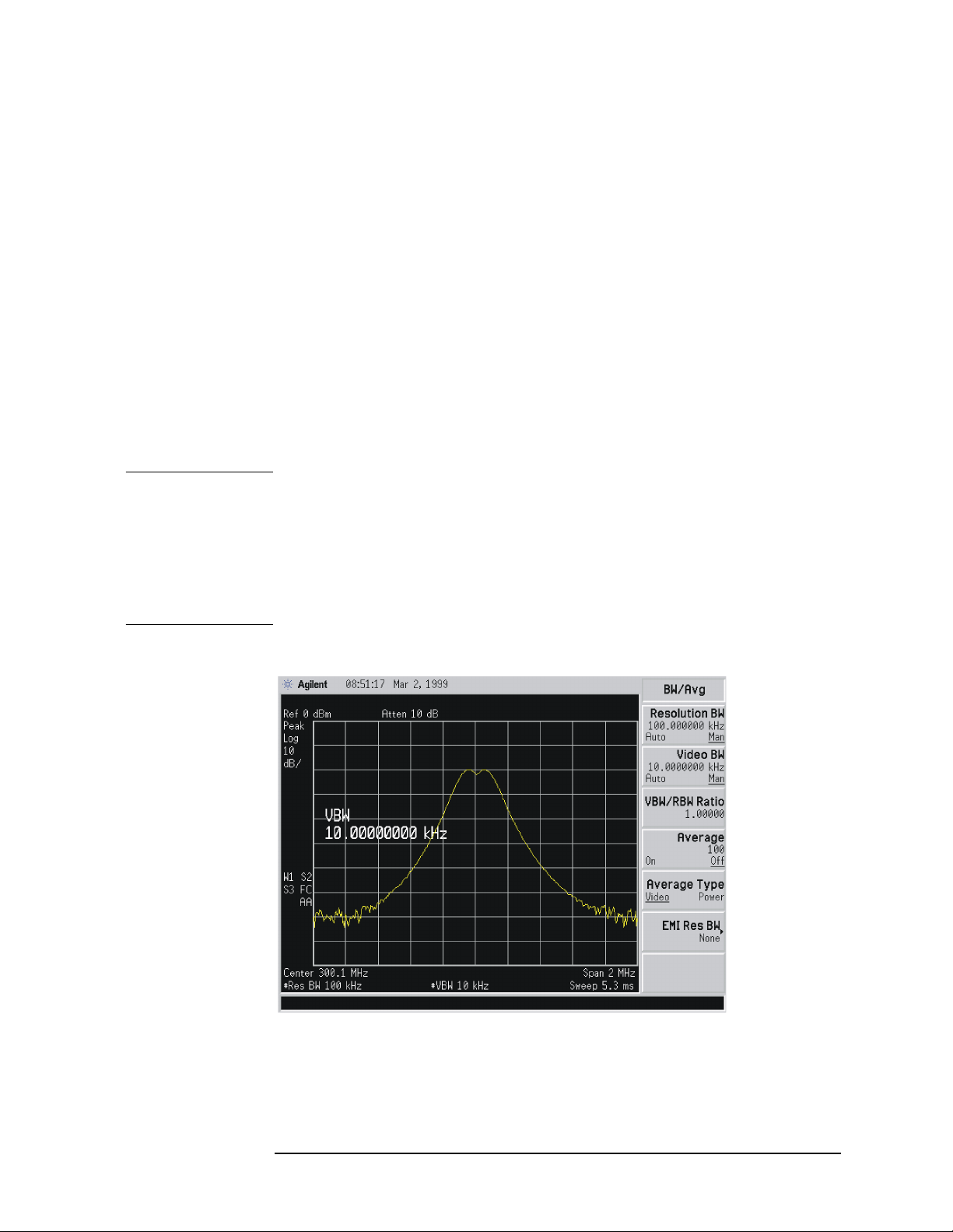
Making Complex Measurements

Making Stimulus Response Measurements

12.Reconnect the DUT to the analyzer. Note that the units of the
reference level have changed to dB, indicating that this is now a
relative measurement.

Press

Trace/View, More, Normal i ze, Norm Ref Posn to change the

normalized reference p osition. Arrowheads at the left and right
edges of the grati cul e m ark the normalized reference position, or the
position where 0 dB insertion loss (transmission measurements) or
0 dB return loss (refl ec t io n me asurements) wi ll n o rmally re s ide.
Using the knob results in a change in the position of the normalized
trace, within the range of the graticule.

13.To measure the rejection of the filter 45 MHz above the center of the
bandpass, press
center of the si gnal), and then press

Marker, 200, MHz (to ensure that the marker is i n the

Delta, 45, MHz. The marker

readout displays the rejection of the filter at 45 MHz above the
center of the ba ndpass. See Figure2-4.

NOTE Because the default tra ce is comprised of 401 discrete points, the

indicated marker frequency may differ slightly from the frequency that
you entered. Due to the horizontal resolution of the trace, the marker
frequency value will be r ounded to withi n 0.25% of the span of the v alue
entered. If the analyz e r is an E S A -E se ri e s wi t h firm ware revisi o n
A.04.00 or later, the number of sweep points may be set to any value
betwee n 101 and 8192 .

Figu r e 2- 4 Me a sure the Reje ct i o n Ra n g e

Chapter 2 75

Making Complex Measurements

Making Stimulus Response Measurements

Tracking Generator Unleveled Condition

When using the tracking generator, the message TG unleveled may
appear. The TG unl eve led message indicates that the tracking
generat o r sou rce po wer (
the selected level during some portion of the sweep. If the unleveled
condition exists at the beginning of the sweep, the message will be
displayed immediately. If the unleveled conditi on occurs after the sweep
begins, the m e ssa ge wi ll be disp lay e d after the sweep is co mpleted. A
momentary unleveled condi tion may not be detected when the sweep
time is short. T he message will be cleared after a sweep is completed
with no unleveled conditions.

The unleveled condition may be caused by any of the following:

• Start frequency is too low or the stop frequency is too high. The
unleveled condition is likely to occur if the true frequency range
exceeds the tracking g enerator frequency specification (especially
the low frequency speci fication).

• Source attenuation may be set incorr ectly (select
for optimum setting).

• The source power may be set too high or too low, use
then Amplitude (On) to reset it.

• The source power sweep may be set too hi gh, resulting in an
unleveled condition at the end of the sweep. Use
then

Power Sweep (On) to decrease the amplitude.

• Reverse RF power from the device under test detected by the
tracki n g generat o r A LC (auto matic leve l control ) s ystem.

Source, Amplitude) could not be maintained at

Attenuation (Auto )

Amplitude (Off)

Power Sweep (Off)

Measuring Device Bandwidth

It is often nec essary to m easure dev ice bandwidth, such as w hen testing
a bandpass filter. There is a key in the
perform this function. The device signal being measured must be
displayed before activating the measurement. The span must include
the full respons e.

Activate the measurement by toggling the
analyzer places arrow marker s at the −3 dB points on either side of the
response an d re ads the bandwidth. For oth e r bandwidth re spo n se s
enter the numb e r o f dB do w n desired, from −1 dB t o −80 dB.

No other signal can app ear on the display within N dB of the highest
signal. Th e me asured sig n al cannot h ave more th an o n e pea k t h at is
greater than or equal to N dB. A signal must have a peak greater than
the currently defined peak excursion to be identifi ed . The default value
for the peak excursi on is 6 dB.

Peak Search menu that will

N dB Points key to O n. The

76 Chap ter 2

Making Stimulus Response Measurements

Measurements are made continuously, updating at the end of each
sweep. Thi s all o ws y o u to ma ke adj u st m e nts a n d se e chan ges as they
happen. The single sweep mode can also be used, providing time to
study or re co rd the data.

The N dB bandwidth measurement error is typically ±1% of the span.

Example:

Measure th e 3 dB ban dwidth of a 200 MHz ban dpass filter.

1. T o measu re the rejection of a bandpass filter, connect the equipment
as shown in Figure 2-5. This ex am ple uses a 20 0 M H z bandpass
filter.

Figure 2-5 Transmission Measurement Test Setup

Making Complex Measurements

2. Perform a factory preset by pres sing

Preset, Factory Preset (if

present).

3. Set the Y-Axis Units to dBm by pressing

Y-Axis Units,

dBm.

4. Set the span to 100 MHz by pressing

5. Set the cen ter frequen c y to 200 MHz by pressi n g

Center Freq, 200, MHz.

6. Set the resolution bandwidth to 10 kHz by pressing

AMPLITUDE, More,

SPAN, Span, 100, MHz.

FREQUENCY,

BW/Avg, Res B W,

10, kHz.

7. Turn on the tracking generator and if necessary, set the output
power to –10 dBm by pressi n g

CAUTION Excessive signal input may damage the DUT. Do not exceed the

Source, Amplitude (On), –10, dBm.

maximu m power that t h e d e vi ce under test ca n tolerate.

Chapter 2 77

Making Complex Measurements

Making Stimulus Response Measurements

NOTE To reduce ripples caused by source return loss, use 10 dB (E7401A) or 8

dB (all other m odels) or greater tracking genera tor output attenuation.
Tracking generator output attenuation is norma lly a function of the
source power selected . However, the output attenuation may be
controll ed in the

Source menu. Refer to specific ations and

charac teristics in your spe cificatio n s gu ide for m o re in fo rmation on the
relationsh ip between so u rce po wer and source atten ua t ion .

8. Put the sweep time of the analyzer into stimulus response auto
coupled mo de by pre ssi n g

Sweep, then Swp Cou p l ing (SR). Auto

coupled sweep times are usually much faster for stimulus response
measurements than they are f or spectrum analyzer (SA)
measurements. Adjust the reference level if necessary to p lace the
signal on screen.

NOTE In the stimulus resp onse mode, the Q of the DUT can determine the

fastest rate at whic h the a nalyzer c an be swept. ( Q is the q uality factor,
which is the center frequency of the DUT divided by the bandwidth of
the DUT.) To determine whether the analyzer is swee ping too fast, slow
the sweep and note w hether there is a frequency or amplitude shift of
the trace. Continue to slow the sweep until there is no longer a
frequency or amplitude shift.

9. To activate the N dB bandwidth function press
then

N dB Points (On). See Figure 2-6.

10.Read the measurement results d isplayed on the screen.

Figure 2-6 N dB Bandwidth Measurement at –3 dB

Peak Search, More,

78 Chap ter 2

Making Stimulus Response Measurements

11.The knob or the data entry keys can be used to change the N dB
value from −3 dB to −60 dB to measure the 60 dB bandwidth of the
filter. See Figure 2-7.

Figure 2-7 N dB Bandwidth Measurement at –60 dB

Making Complex Measurements

12.Press

N dB Points (Off) to turn the meas urement off.

Measuring Stop Band Attenuation Using Log Sweep

When measuring filter charac teristics, it is useful to look at the
stimulus response over a wide frequency range. Setting the analy zer
x-axis (frequency) to display logarithmically provides this function.

Example:

Measure the stop band attenuation of a 10 MHz low pass filter.

1. To measure the response of a low pass filter, connect the equipment
as shown in Figure 2-8. This example uses a 10 MHz low pass filter.

Chapter 2 79

Making Complex Measurements

Making Stimulus Response Measurements

Figure 2-8 Transmission Measurement Test Setup

2. Perform a factory preset by pressing

Preset, Factory Preset (if

present).

3. Se t th e Y-Axis Units to dBm by pressing

Y-Axis Units,

dBm.

4. Set the st art frequen cy to 100 kHz by pressing

Start Freq, 10 0, kHz.

5. Set the stop frequency to 1 GHz by pressing

6. Set the resolution bandwidth to 10 kHz by pressing

AMPLITUDE, More,

FREQUENCY,

Stop Fr eq, 1, GHz.

BW/Avg, Res B W,

10, kHz.

7. Set the frequency scale to log by pressing

Scale Type (Log).

FREQUENCY,

8. For E7405A analyzers with Option UKB, set the i nput coupling to
DC by pressi n g

Input, Coupling (DC).

9. Turn on the tracking generat o r and if necessa ry, set the output
power to –10 dBm by pressing

CAUTION Excessive signal input may damage the DUT. Do not exceed the

Source, Amplitude (On), –10, dBm.

maximu m po wer that the de vice under t e st can to le rate.

NOTE To reduce ripples caused by source return loss, use 10 dB (E7401A) or 8

dB (all other m odels) or greater tracking genera tor output attenuation.
Tracking generator output attenuation is norma lly a function of the
source power selected . However, the output attenuation may be
controll ed in the

Source menu. Refer to specifications and

charac teristics in your spe cificatio n s gu ide for m o re in fo rmation on the
relationsh ip between so u rce po wer and source atten ua t ion .

80 Chap ter 2

Making Complex Measurements

Making Stimulus Response Measurements

Figure 2-9 Tracking Generator Output Power Activated in Log Sweep

10.Put the sweep time of the analyzer into stimulus response auto
coupled mode by pre s sing

Sweep, then Swp Coupling (SR). See

Figure 2-9. Auto coupled sweep times are usually much fa ster for

stimulus response measurem ents than they are for spectrum
analyze r (SA) measurements. Adjust the reference level if necessary
to place the signal on screen.

11.To make a transmission measurement accurately, the frequency
response of t he test system must be known. Normalization is used to
eliminate this er ror from the measurement. To measure the
frequency response of the test system, connect the cable ( but not the
DUT) from the tracking generator output to the analyzer input.
Press

Trace/View, More, Normalize, Store Ref (1→3), Normalize (On).

This will activate the trace 1 minus trace 3 function and display the
results in trace 1. The normalized trace or flat line represents 0 dB
return loss. N o rmaliza t io n o ccu rs each swe ep.

NOTE Since the calibration trace is stored in trace 3, changing trace 3 to

Clear Write, Max Hold, or Min Hold will invalidate the normalization.

12.Reconnect the DUT to the analyzer. Note that the units of the
reference level have changed to dB, indicating that this is now a
relative measurement. Refer to Figure 2-10.

13.Press

Trace/View, More, Normalize, Norm Ref Posn to change the

normalized reference p osition. Arrowheads at the left and right
edges of the graticule mark the normalized reference position. Using
the knob results in a change in the position of the normali zed trace,
within the range of the graticule. Refer to Figure 2-10.

Chapter 2 81

Making Complex Measurements

Making Stimulus Response Measurements

Figure 2-10 Normalized Trace After Reconnecting DUT

14.Press

Marker, Delta Pair (R e f), 10, MHz to place the reference marker

at the specified cutoff frequency.

15.Press

Delta Pair (∆), 20 , MHz to place the second marker at the

20 MHz point. In this example, the attenuation over this frequency
range is 63.32 dB/octave (one octave ab ove the cutoff frequency).

Figure 2-11 Determining Low Pass Filter Rolloff

16.Use the knob to place the m arker at the highest peak in the stop
band to determine the minimum stop band attenuation. In this
exampl e, t h e pe ak o ccu rs at 708.76 MHz . T h e atte n u ation is

54.92 dB.

82 Chap ter 2

Figure 2-12 Minimum Stop Band Attenuation

Making Complex Measurements

Making Stimulus Response Measurements

Chapter 2 83

Making Complex Measurements

Making a Reflection C alibration Measurement

Making a Reflection Calibration Measurement

The calibration standard for reflecti on measurements is usually a short
circuit conn e ct e d at the refere n ce plane (the po in t at wh ich the dev ice
under test (DUT) will be connected.) See Figure 2-13. A short circuit
has a reflection coeffic ient of 1 (0 dB return loss) . It r ef lects all i ncid ent
power and pr ov id e s a co n ve n i e n t 0 dB refe re n ce .

Figure 2-13 Reflection Measurement Short Calibration Test Setup

Example:

Measure the return loss of a filter. The following procedure makes a
reflection measurement using a coupler or directional bridge. This
example uses a 200 MHz bandpass filter as the DU T.

NOTE The analyzer center frequency and span for this measurement can

easily be set up using the transmission measurement setup in “Making

Stimulus Response Meas urements” on page 71. Tune the analyzer so

that the passband of the filter comprises a majority of the display, then
proceed with the steps outlined below.

84 Chap ter 2

Making Complex Measurements

Making a Reflection Calibration Measurement

Reflection Calibration

1. Connect th e DUT to the direction al bridge or coupler as shown in

Figure 2-13. Ter m inate the unconnected port of the DUT.

NOTE If possible , use a co u pler or bridg e with the correct t e st po rt co n n ect o r

for both cal ibrating an d measurin g . An y adapter be t we e n t h e te st po rt
and DUT degrades coupler/bridge directivity and system source match.
Ideally, you should use the same adapter for the calibration and the
measurement. Be sure to termi nate the second port of a t wo port devic e.

2. Connect the tracking generator output of the analyzer to the
directional bridge or coupler.

3. Connect the analyzer input to the coupled port of the directional
bridge or coupler.

4. Perform a factory preset by pres sing

Preset, Factory Preset (if

present).

5. Set the Y-Axis Units to dBm by pressing

Y-Axis Units,

dBm.

AMPLITUDE, More,

6. Turn on the tracking generator and if necessary, set the output
power to –10 dBm by pressi n g

CAUTION Excessive signal input may damage the DUT. Do not exceed the

Source, Amplitude (On), –10, dBm.

maximu m power that t h e d e vi ce under test ca n tolerate.

7. Set the span to 100 MHz by pressing

8. Set the cen ter frequen c y to 200 MHz by pressi n g

Center Freq, 200, MHz.

9. Set the resolution bandwidth to 3 MHz by pressing

SPAN, Span, 100, MHz.

FREQUENCY,

BW/Avg, Res BW,

3, MHz.

10.Replace the DUT with a short circuit.

11.Normalize the trace by pressing

Store Ref (1→3), Normalize (On). See Figure 2-14.

Trace/View, More, Normalize,

This will activate the trace 1 minus trace 3 function and display the
results in trace 1. The normalized trace or flat line represents 0 dB
return loss. No rmaliza t io n o ccu rs each swe ep. Replace th e sh o rt
circuit wit h the D U T.

NOTE Since the reference trace is stored in trace 3, changi ng trace 3 to

Clear Write will in validate the normaliza t ion.

Chapter 2 85

Making Complex Measurements

Making a Reflection C alibration Measurement

Figure 2-14 Short Circuit Normalized

Measuring the Return Loss

1. After calibrating the system with the above procedure, r econnect the
filter in place of the short circuit without changing any analyzer
settings.

2. Use the marker to read return loss. Press
marker with the knob to r ead the return loss at that frequenc y. Or
you can use the Min Search function to measure return loss by
pressing
the point where the return loss is maximized. See Figure 2-15.

Figure 2-15 Measuring the Return Loss of the Filter

Peak Search, Min Search, the analyzer will place a marker at

Marker and position th e

86 Chap ter 2

Converti ng Return Loss to VSWR

VSWR

110

RL–

20

----------

+

110

RL–

20

----------

–

-----------------------=

Return loss can be expressed as a voltage standing wave ratio (VSWR)
value using the following table or formula:

Table 2-1 Power to VSWR Conversion

Making Complex Measurements

Making a Reflection Calibration Measurement

Return

Loss
(dB)

4.0 4.42 14.0 1.50 18.0 1.29 28.0 1.08 38.0 1.03

6.0 3.01 14.2 1.48 18.5 1.27 28.5 1.08 38.5 1.02

8.0 2.32 14.4 1.47 19.0 1.25 29.0 1.07 39.0 1.02

10.0 1.92 14.6 1.46 19.5 1.24 29.5 1.07 39.5 1.02

10.5 1.85 14.8 1.44 20.0 1.22 30.0 1.07 40.0 1.02

11.0 1.78 15.0 1.43 20.5 1.21 30.5 1.06 40.5 1.02

11.2 1.76 15.2 1.42 21.0 1.20 31.0 1.06 41.0 1.02

11.4 1.74 15.4 1.41 21.5 1.18 31.5 1.05 41.5 1.02

11.6 1.71 15.6 1.40 22.0 1.17 32.0 1.05 42.0 1.02

11.8 1.69 15.8 1.39 22.5 1.16 32.5 1.05 42.5 1.02

12.0 1.67 16.0 1.38 23.0 1.15 33.0 1.05 43.0 1.01

12.2 1.65 16.2 1.37 23.5 1.14 33.5 1.04 43.5 1.01

12.4 1.63 16.4 1.36 24.0 1.13 34.0 1.04 44.0 1.01

VSWR Return

Loss
(dB)

VSWR Return

Loss
(dB)

VSWR Return

Loss
(dB)

VSWR Return

Loss
(dB)

VSWR

12.6 1.61 16.6 1.35 24.5 1.13 34.5 1.04 44.5 1.01

12.8 1.59 16.8 1.34 25.0 1.12 35.0 1.04 45.0 1.01

13.0 1.58 17.0 1.33 25.5 1.11 35.5 1.03 45.5 1.01

13.2 1.56 17.2 1.32 26.0 1.11 36.0 1.03 46.0 1.01

13.4 1.54 17.4 1.31 26.5 1.10 36.5 1.03 46.5 1.01

13.6 1.53 17.6 1.30 27.0 1.09 37.0 1.03 47.0 1.01

13.8 1.51 17.8 1.30 27.5 1.09 37.5 1.03 47.5 1.01

Where: RL is the measured r eturn loss value.
VSWR is sometimes stated as a ratio. For example: 1.2:1 “one point two

to one” VSWR. The first number is the VSWR value taken from the
table or calculate d u sing the for mu la. The seco n d n u mber is alw ays 1.

Chapter 2 87

Making Complex Measurements

Demodulating and Listening to an AM Signal

Demodulating and Listening to an AM Signal

The functions listed in the menu under Det/Demod allow yo u to
demodulate and hear signal information displayed on the analyzer.
Simply place a mark er on a signal of interest, activate AM
demodulation, turn the speaker on, and then listen.

Demodulating and Listening to an AM Signal Example 1:

1. Connect an antenna to the analyzer input.

2. Perform a factory preset by pressing
present).

3. Se t th e Y-Axis Units to dBm by pressing

Y-Axis Units,

dBm.

4. Select a frequency range on the analyzer, such as the range for AM
radio broadcasts. For examp le, the frequency range for AM
broadcasts in the United States is 550 kHz to 1650 kHz. Press

FREQUENCY, Start Freq, 550, kHz, Sto p F req, 1650, kHz.

5. Place a marker on the sig nal of i nter es t. Press
marker on the highest amplitude si gnal, or p r ess
move the marker to a signal of interest. See Figure 2-16.

6. Press

Det/Demod, Demod, AM. Use the front-panel volume knob to

control the speaker volume.

Figure 2-16 Demodulation of an AM Signal

Preset, Factory Preset (if

AMPLITUDE, More,

Peak Search to place a

Marker, Normal and

88 Chap ter 2

Making Complex Measurements

Demodulating and Listeni ng to an AM Signal

7. Th e signal is demo dulated at the marker position on ly fo r t h e
duration of the demod tim e. Use the step keys, knob, or numeric
keypad to change the dwell time. F or e xample, press the s tep up key
(↑) to increase the dwel l time to 2 seconds.

8. The marker search functions can b e used to move the marker to
other signals of interest. Press

Next Pk Right, or Next Pk Left.

Peak Search to access Next Peak,

Demodulating and Listening to an AM Signal Example 2:

1. Connect an antenna to the analyzer input.

2. Perform a factory preset by pres sing

Preset, Factory Preset (if

present).

3. Select a frequency range on the analyzer, s uch as the range for AM
radio broadcasts. For example, the frequency range for AM
broadcast s in t h e U n it e d States is 55 0 k H z t o 1650 kHz. Pr es s

FREQUENCY, Start Freq, 55 0, kHz, Stop Freq, 16 50, kHz.

4. Place a marker on the signal of interest. Press

Peak Search to place a

marker on the highest amplitud e signal , or pres s Marker, Normal and
move the marker to a signal of interest.

5. Set the resolution bandwidth to spectrum analyzer by pressing

BW/Avg and Res BW (SA).

6. Set the frequency of the si gnal to center frequency by pressi ng

FREQUENCY then Signal Track (On) if the signal of interest is the

highest amplitude on screen signal. If it is not the highest amplitud e
signal on screen, move the signal to center screen by pressing

Peak Search, Marker→, and Mkr→CF.

7. If the signal track function is on, press

SPAN, 1, MHz to reduce the

span to 1 MHz. If signal track is not used, use the step down key (↓)
to reduce the spa n and use Mkr→CF to keep the signal of interest at
center screen.

8. Set the span to zero by pressing

SPAN, Zero Span. Zero Span turns off

the signal track function.

9. C h an g e the reso lution bandwidth to 100 k H z by pressing

Res BW, then enter 100, kHz.

BW/Avg,

10.Set the signal i n the top two divisions of the screen by changing the
reference level. Press

AMPLITUDE, and then the step d own key (↓)

until the sig nal is in the top two divisio ns. Set the amplitude scale to
linear by pressing Scale Type (Lin). Keep the signal center displayed
by pressing AMPLITUDE, Ref Level and using the (↑) (↓) ste p k e ys.

Chapter 2 89

Making Complex Measurements

Demodulating and Listening to an AM Signal

11.Press Det/Demod, Detector, Sample to set the detector mode of the
analyzer to Sample.

12.Press

Det/Demod, Demod, AM. Use the front panel volum e knob to

control the speaker volume.

13.You can turn your analyzer into a % AM indicator as follows:
a. Set trigger to free run b y pressing Trig, Free Run.

b. S e t the swe ep time to 5 second s by pre ssi n g

Sweep Time,5,s.

c. Set the video filter to 30 Hz by pressing

Sweep,

BW/Avg, Video BW, 30, Hz.

d. Change the reference level to position the trace at midscreen by

pressing

AMPLITUDE, Ref Level, and adjust the reference level

using the front-panel knob.

e. Reset the video filter to a high value. For example, press

Video B W, 30, kHz.

f. Set the sweep time to 5 milli seconds by pressing

, 5, ms.

Time

Sweep, Sweep

BW/Avg,

The center horizontal line of the graticule now represents 0% AM;
the top and bottom lines, 100% AM. See Figure 2-17.

14.The signal to the speaker will be interrupted during r etr ace b ecause
the analyzer is perf orming automatic alignment routines. To
eliminate the interruption and clicks between sweeps, turn the auto
alignment function off by pressing

Off.

System, Alignments, Auto Align,

NOTE Refer to the specificat ions f or infor mation about opera ting the anal yzer

with the alignments turned off.

90 Chap ter 2

Demodulating and Listeni ng to an AM Signal

Figure 2-17 Continuous Demodulation of an AM Signal

Making Complex Measurements

Chapter 2 91

Making Complex Measurements

Demodulating and Listening to an AM Signal

92 Chap ter 2