Native Instruments Reaktor Core Instruction Manual

REAKTOR CORE

Tutorial

The information in this document is subject to change without notice and does not represent a commitment on the part of Native Instruments Software Synthesis GmbH. The software described by this document is subject to a License Agreement and may not be copied to other media. No part of this publication may be copied, reproduced or otherwise transmitted or recorded, for any purpose, without prior written permission by Native Instruments Software Synthesis GmbH. All product and company names are trademarks of their respective owners.

And also, if you’re reading this, it means you bought the software rather than stole it. It’s because of people like you that we can continue to create great tools and update them. So, thank you very much.

Manual written by NI and Len Sasso

REAKTOR, REAKTOR 5 and REAKTOR CORE are a trademarks of Native Instruments Software Synthesis.

Germany USA

Native Instruments GmbH Native Instruments USA, Inc. Schlesische Str. 28 5631 A Hollywood Boulevard D-10997 Berlin Los Angeles, CA 90028 Germany USA info@native-instruments.de info@native-instruments.com www.native-instruments.de www.native-instruments.com

Table of Contents

1. First steps in Reaktor Core ..................................................................... 11

1.1. What is Reaktor Core ...............................................................11

1.2. Using core cells .......................................................................12

1.3. Using core cells in a real example ..............................................15

1.4. Basic editing of core cells .........................................................17

2. Getting into Reaktor Core ......................................................................22

2.1. Event and audio core cells ....................................................... 22

2.2. Creating your ﬁrst core cell .......................................................24

2.3. Audio and control signals ........................................................ 36

2.4. Building your ﬁrst Reaktor Core macros ..................................... 42

2.5. Using audio as control signal ....................................................49

2.6. Event signals .......................................................................... 50

2.7. Logic signals .......................................................................... 54

3. Reaktor Core fundamentals: the core signal model .................................56

3.1. Values ................................................................................... 56

3.2. Events ................................................................................... 56

3.3. Simultaneous events ............................................................... 59

3.4. Processing order .....................................................................61

3.5. Event core cells reviewed ......................................................... 62

4. Structures with internal state ................................................................68

4.1. Clock signals .......................................................................... 68

4.2. Object Bus Connections .......................................................... 69

4.3. Initialization ............................................................................72

4.4. Building an event accumulator ..................................................75

4.5. Event merging .........................................................................76

4.6. Event accumulator with reset and initialization ........................... 78

4.7. Fixing the event shaper ............................................................ 84

5. Audio processing at its core ..................................................................87

5.1. Audio signals .......................................................................... 87

5.2. Sampling rate clock bus .......................................................... 89

5.3. Connection feedback .............................................................. 90

5.4. Feedback around macros ......................................................... 93

5.5. Denormal values ..................................................................... 97

5.6. Other bad numbers ................................................................ 101

5.7. Building a 1-pole low pass ﬁlter ............................................... 101

REAKTOR CORE – III

6. Conditional processing ........................................................................ 105

6.1. Event routing .........................................................................105

6.2. Building a signal clipper ......................................................... 107

6.3. Building a simple sawtooth oscillator .......................................108

7. More signal types ................................................................................ 110

7.1. Float signals .......................................................................... 110

7.2. Integer signals .......................................................................112

7.3. Building an event counter ....................................................... 114

7.4. Building a rising edge counter macro ........................................ 116

8. Arrays ................................................................................................. 119

8.1. Introduction to arrays ............................................................. 119

8.2. Building an audio signal selector .............................................122

8.3. Building a delay ....................................................................128

8.4. Tables ................................................................................. 134

9. Building optimal structures .................................................................. 139

9.1. Latches and modulation macros ..............................................139

9.2. Routing and merging ..............................................................140

9.3. Numerical operations ............................................................. 141

9.4. Conversions between ﬂoats and integers ..................................141

Appendix A. Reaktor Core user interface ..................................................143

A.1. Core cells .............................................................................143

A.2. Core modules/macros ............................................................143

A.3. Core ports ............................................................................144

A.4. Core structure editing ............................................................144

Appendix B. Reaktor Core concept ...........................................................145

B.1. Signals and events .................................................................145

B.2. Initialization ..........................................................................145

B.3. OBC connections ..................................................................145

B.4. Routing ................................................................................145

B.5. Latching ...............................................................................146

B.6. Clocking ...............................................................................146

Appendix C. Core macro ports .................................................................. 147

C.1. In ........................................................................................ 147

C.2. Out ...................................................................................... 147

C.3. Latch (input) .........................................................................147

C.4. Latch (output) ....................................................................... 147

C.5. Bool C (input) .......................................................................147

C.6. Bool C (output) .....................................................................148

IV – REAKTOR CORE

Appendix D. Core cell ports .....................................................................149

D.1. In (audio mode) .....................................................................149

D.2. Out (audio mode) ..................................................................149

D.3. In (event mode) ....................................................................149

D.4. Out (event mode) ..................................................................149

Appendix E. Built-in busses .....................................................................150

E.1. SR.C ....................................................................................150

E.2. SR.R ....................................................................................150

Appendix F. Built-in modules .................................................................... 150

F.1. Const ....................................................................................150

F.2. Math > + ..............................................................................150

F.3. Math > - ............................................................................... 151

F.4. Math > * ............................................................................... 151

F.5. Math > / ...............................................................................151

F.6. Math > |x| .............................................................................151

F.7. Math > –x ..............................................................................151

F.8. Math > DN Cancel .................................................................152

F.9. Math > ~log ..........................................................................152

F.10. Math > ~exp ........................................................................152

F.11. Bit > Bit AND ......................................................................152

F.12. Bit > Bit OR ........................................................................153

F.13. Bit > Bit XOR ......................................................................153

F.14. Bit > Bit NOT ......................................................................153

F.15. Bit > Bit << .........................................................................153

F.16. Bit > Bit >> .........................................................................154

F.17. Flow > Router ......................................................................154

F.18. Flow > Compare ...................................................................154

F.19. Flow > Compare Sign ............................................................154

F.20. Flow > ES Ctl ......................................................................155

F.21. Flow > ~BoolCtl ...................................................................155

F.22. Flow > Merge ......................................................................155

F.23. Flow > EvtMerge ..................................................................156

F.24. Memory > Read ...................................................................156

F.25. Memory > Write ...................................................................156

F.26. Memory > R/W Order ...........................................................156

F.27. Memory > Array ...................................................................157

F.28. Memory > Size [ ] ................................................................157

F.29. Memory > Index ..................................................................157

F.30. Memory > Table ...................................................................158

F.31. Macro .................................................................................158

REAKTOR CORE – V

Appendix G. Expert macros ...................................................................... 159

G.1. Clipping > Clip Max / IClip Max ...............................................159

G.2. Clipping > Clip Min / IClip Min ................................................159

G.3. Clipping > Clip MinMax / IClipMinMax .....................................159

G.4. Math > 1 div x ......................................................................159

G.5. Math > 1 wrap ......................................................................159

G.6. Math > Imod ........................................................................160

G.7. Math > Max / IMax ................................................................160

G.8. Math > Min / IMin .................................................................160

G.9. Math > round ........................................................................160

G.10. Math > sign +- ....................................................................160

G.11. Math > sqrt (>0) .................................................................160

G.12. Math > sqrt ........................................................................161

G.13. Math > x(>0)^y ..................................................................161

G.14. Math > x^2 / x^3 / x^4 ........................................................161

G.15. Math > Chain Add / Chain Mult ............................................. 161

G.16. Math > Trig-Hyp > 2 pi wrap ................................................. 161

G.17. Math > Trig-Hyp > arcsin / arccos / arctan ..............................161

G.18. Math > Trig-Hyp > sin / cos / tan ...........................................162

G.19. Math > Trig-Hyp > sin –pi..pi / cos –pi..pi / tan –pi..pi .............162

G.20. Math > Trig-Hyp > tan –pi4..pi4 ...........................................162

G.21. Math > Trig-Hyp > sinh / cosh / tanh .....................................162

G.22. Memory > Latch / ILatch ......................................................162

G.23. Memory > z^-1 / z^-1 ndc ....................................................162

G.24. Memory > Read [] ...............................................................163

G.25. Memory > Write [] ...............................................................163

G.26. Modulation > x + a / Integer > Ix + a .....................................163

G.27. Modulation > x * a / Integer > Ix * a ......................................163

G.28. Modulation > x – a / Integer > Ix – a ......................................164

G.29. Modulation > a – x / Integer > Ia – x ......................................164

G.30. Modulation > x / a ...............................................................164

G.31. Modulation > a / x ...............................................................164

G.32. Modulation > xa + y .............................................................164

Appendix H. Standard macros .................................................................. 165

H.1. Audio Mix-Amp > Amount ......................................................165

H.2. Audio Mix-Amp > Amp Mod ...................................................165

H.3. Audio Mix-Amp > Audio Mix ...................................................165

H.4. Audio Mix-Amp > Audio Relay ................................................165

H.5. Audio Mix-Amp > Chain (amount) ...........................................166

H.6. Audio Mix-Amp > Chain (dB) ..................................................166

VI – REAKTOR CORE

H.7. Audio Mix-Amp > Gain (dB) ....................................................166

H.8. Audio Mix-Amp > Invert .........................................................167

H.9. Audio Mix-Amp > Mixer 2 … 4 ...............................................167

H.10. Audio Mix-Amp > Pan ..........................................................167

H.11. Audio Mix-Amp > Ring-Amp Mod ..........................................167

H.13. Audio Mix-Amp > Stereo Mixer 2 … 4 ...................................168

H.14. Audio Mix-Amp > VCA ..........................................................168

H.15. Audio Mix-Amp > XFade (lin) ................................................ 169

H.16. Audio Mix-Amp > XFade (par) ...............................................169

H.17. Audio Shaper > 1+2+3 Shaper ..............................................169

H.18. Audio Shaper > 3-1-2 Shaper ...............................................169

H.19. Audio Shaper > Broken Par Sat ............................................. 170

H.20. Audio Shaper > Hyperbol Sat ...............................................170

H.21. Audio Shaper > Parabol Sat .................................................170

H.22. Audio Shaper > Sine Shaper 4 / 8 ......................................... 171

H.23. Control > Ctl Amount ..........................................................171

H.24. Control > Ctl Amp Mod ........................................................171

H.25. Control > Ctl Bi2Uni ............................................................ 171

H.26. Control > Ctl Chain .............................................................172

H.27. Control > Ctl Invert ..............................................................172

H.28. Control > Ctl Mix ................................................................172

H.29. Control > Ctl Mixer 2 ...........................................................172

H.30. Control > Ctl Pan ................................................................173

H.31. Control > Ctl Relay ..............................................................173

H.32. Control > Ctl XFade .............................................................173

H.33. Control > Par Ctl Shaper ......................................................173

H.34. Convert > dB2AF ................................................................ 174

H.35. Convert > dP2FF ................................................................ 174

H.36. Convert > logT2sec .............................................................174

H.37. Convert > ms2Hz ................................................................ 174

H.38. Convert > ms2sec ...............................................................175

H.39. Convert > P2F .................................................................... 175

H.40. Convert > sec2Hz ...............................................................175

H.41. Delay > 2 / 4 Tap Delay 4p ...................................................175

H.42. Delay > Delay 1p / 2p / 4p ...................................................175

H.43. Delay > Diff Delay 1p / 2p / 4p ............................................. 176

H.44. Envelope > ADSR ...............................................................176

H.45. Envelope > Env Follower ......................................................177

H.46. Envelope > Peak Detector ....................................................177

H.47. EQ > 6dB LP/HP EQ ............................................................177

REAKTOR CORE – VII

H.48. EQ > 6dB LowShelf EQ .......................................................177

H.49. EQ > 6dB HighShelf EQ .......................................................178

H.50. EQ > Peak EQ ....................................................................178

H.51. EQ > Static Filter > 1-pole static HP .....................................178

H.52. EQ > Static Filter > 1-pole static HS .....................................178

H.53. EQ > Static Filter > 1-pole static LP ......................................179

H.54. EQ > Static Filter > 1-pole static LS ......................................179

H.55. EQ > Static Filter > 2-pole static AP .....................................179

H.56. EQ > Static Filter > 2-pole static BP .....................................179

H.57. EQ > Static Filter > 2-pole static BP1 .................................... 179

H.58. EQ > Static Filter > 2-pole static HP .................................... 180

H.59. EQ > Static Filter > 2-pole static HS .................................... 180

H.60. EQ > Static Filter > 2-pole static LP ..................................... 180

H.61. EQ > Static Filter > 2-pole static LS ..................................... 180

H.62. EQ > Static Filter > 2-pole static N .......................................181

H.63. EQ > Static Filter > 2-pole static Pk ......................................181

H.64. EQ > Static Filter > Integrator ..............................................181

H.65. Event Processing > Accumulator ...........................................181

H.66. Event Processing > Clk Div ...................................................182

H.67. Event Processing > Clk Gen ..................................................182

H.68. Event Processing > Clk Rate .................................................182

H.69. Event Processing > Counter ..................................................182

H.70. Event Processing > Ctl2Gate ............................................... 183

H.71. Event Processing > Dup Flt / IDup Flt ................................... 183

H.72. Event Processing > Impulse ................................................. 183

H.73. Event Processing > Random ................................................ 183

H.74. Event Processing > Separator / ISeparator ............................. 183

H.75. Event Processing > Thld Crossing ......................................... 184

H.76. Event Processing > Value / IValue ......................................... 184

H.77. LFO > MultiWave LFO ......................................................... 184

H.78. LFO > Par LFO .................................................................. 184

H.79. LFO > Random LFO .............................................................185

H.80. LFO > Rect LFO .................................................................185

H.81. LFO > Saw(down) LFO .........................................................185

H.82. LFO > Saw(up) LFO ............................................................185

H.83. LFO > Sine LFO ................................................................. 186

H.84. LFO > Tri LFO ................................................................... 186

H.85. Logic > AND ..................................................................... 186

H.86. Logic > Flip Flop ................................................................ 186

H.87. Logic > Gate2L .................................................................. 186

VIII – REAKTOR CORE

H.88. Logic > GT / IGT .................................................................187

H.89. Logic > EQ .........................................................................187

H.90. Logic > GE .........................................................................187

H.91. Logic > L2Clock ..................................................................187

H.92. Logic > L2Gate ...................................................................187

H.93. Logic > NOT ...................................................................... 188

H.94. Logic > OR ........................................................................ 188

H.95. Logic > XOR ...................................................................... 188

H.96. Logic > Schmitt Trigger ...................................................... 188

H.97. Oscillators > 4-Wave Mst ..................................................... 188

H.98. Oscillators > 4-Wave Slv ......................................................189

H.99. Oscillators > Binary Noise ....................................................189

H.100. Oscillators > Digital Noise ..................................................189

H.101. Oscillators > FM Op ...........................................................190

H.102. Oscillators > Formant Osc ..................................................190

H.103. Oscillators > MultiWave Osc ................................................190

H.104. Oscillators > Par Osc .........................................................190

H.105. Oscillators > Quad Osc .......................................................191

H.106. Oscillators > Sin Osc .........................................................191

H.107. Oscillators > Sub Osc 4 ......................................................191

H.108. VCF > 2 Pole SV ...............................................................191

H.109. VCF > 2 Pole SV C ............................................................192

H.110. VCF > 2 Pole SV (x3) S ......................................................192

H.111. VCF > 2 Pole SV T (S) ........................................................192

H.112. VCF > Diode Ladder ...........................................................193

H.113. VCF > D/T Ladder .............................................................193

H.114. VCF > Ladder x3 ...............................................................193

Appendix I. Core cell library ....................................................................194

I.1. Audio Shaper > 3-1-2 Shaper ...................................................194

I.2. Audio Shaper > Broken Par Sat ................................................194

I.3. Audio Shaper > Hyperbol Sat ...................................................194

I.4. Audio Shaper > Parabol Sat .....................................................195

I.5. Audio Shaper > Sine Shaper 4/8 ..............................................195

I.6. Control > ADSR .....................................................................195

I.7. Control > Env Follower .............................................................196

I.8. Control > Flip Flop .................................................................196

I.9. Control > MultiWave LFO .........................................................196

I.10. Control > Par Ctl Shaper ........................................................197

I.11. Control > Schmitt Trigger .......................................................197

I.12. Control > Sine LFO ...............................................................197

REAKTOR CORE – IX

I.13. Delay > 2/4 Tap Delay 4p ......................................................198

I.14. Delay > Delay 4p ..................................................................198

I.15. Delay > Diff Delay 4p ............................................................198

I.16. EQ > 6dB LP/HP EQ .............................................................198

I.17. EQ > HighShelf EQ ................................................................199

I.18. EQ > LowShelf EQ ................................................................199

I.19. EQ > Peak EQ ......................................................................199

I.20. EQ > Static Filter > 1-pole static HP ......................................199

I.21. EQ > Static Filter > 1-pole static HS ...................................... 200

I.22. EQ > Static Filter > 1-pole static LP ...................................... 200

I.23. EQ > Static Filter > 1-pole static LS ...................................... 200

I.24. EQ > Static Filter > 2-pole static AP ...................................... 200

I.25. EQ > Static Filter > 2-pole static BP .......................................201

I.26. EQ > Static Filter > 2-pole static BP1 .....................................201

I.27. EQ > Static Filter > 2-pole static HP .......................................201

I.28. EQ > Static Filter > 2-pole static HS ......................................201

I.29. EQ > Static Filter > 2-pole static LP ...................................... 202

I.30. EQ > Static Filter > 2-pole static LS ...................................... 202

I.31. EQ > Static Filter > 2-pole static N ........................................ 202

I.32. EQ > Static Filter > 2-pole static Pk ...................................... 202

I.33. Oscillator > 4-Wave Mst ....................................................... 203

I.34. Oscillator > 4-Wave Slv ........................................................ 203

I.35. Oscillator > Digital Noise ...................................................... 204

I.36. Oscillator > FM Op .............................................................. 204

I.37. Oscillator > Formant Osc ...................................................... 204

I.38. Oscillator > Impulse ............................................................ 204

I.39. Oscillator > MultiWave Osc ................................................... 205

I.40. Oscillator > Quad Osc .......................................................... 205

I.41. Oscillator > Sub Osc ............................................................ 205

I.42. VCF > 2 Pole SV C .............................................................. 206

I.43. VCF > 2 Pole SV T ............................................................... 206

I.44. VCF > 2 Pole SV x3 S ...........................................................207

I.45. VCF > Diode Ladder .............................................................207

I.46. VCF > D/T Ladder ............................................................... 208

I.47. VCF > Ladder x3 .................................................................. 208

Index ......................................................................................................209

X – REAKTOR CORE

1. First steps in Reaktor Core

1.1. What is Reaktor Core

Reaktor Core is a new level of functionality within Reaktor with a new and different set of features. Because there is also an older level of functionality, we will hereinafter refer to these two levels as the core level and the primary level, respectively. Also when we say “primary-level structure” we will mean the structure of an instrument or macro, but not the structure of an ensemble. 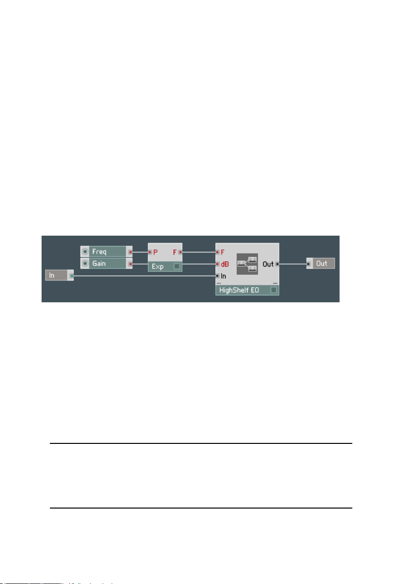The features of Reaktor Core are not directly compatible with those of the primary level, so some interfacing is required between them, and that comes in the form of core cells. Core cells exist inside primary-level structures, and they look similar and behave similarly to primary-level built-in modules. Here is an example structure, using a HighShelf EQ core cell, which differs from the primary-level built-in module version in that it has frequency and boost controls:

Inside of core cells are Reaktor Core structures. Those provide an efﬁcient way to implement custom low-level DSP functionality as well as to build larger-scale signal-processing structures using such functionality. We will take a detailed look at these structures later. Although one of the main purposes of Reaktor Core is to build low level DSP structures, it is not limited to that. For users with little DSP programming experience, we have provided a library of pre-built modules, which you can connect inside core structures, just as you do with ordinary modules and macros in primary-level structures. We have also provided you with a library of pre-built core cells, which are immediately available for you to use in primary-level structures.

In the future, Native Instruments will put less emphasis on creating new primary-level modules. Instead, we will use our new Reaktor Core technology and provide them in the form of core cells. For example, you will already ﬁnd a set of new ﬁlters, envelopes, effects, and so on in the core cell library.

REAKTOR CORE – 11

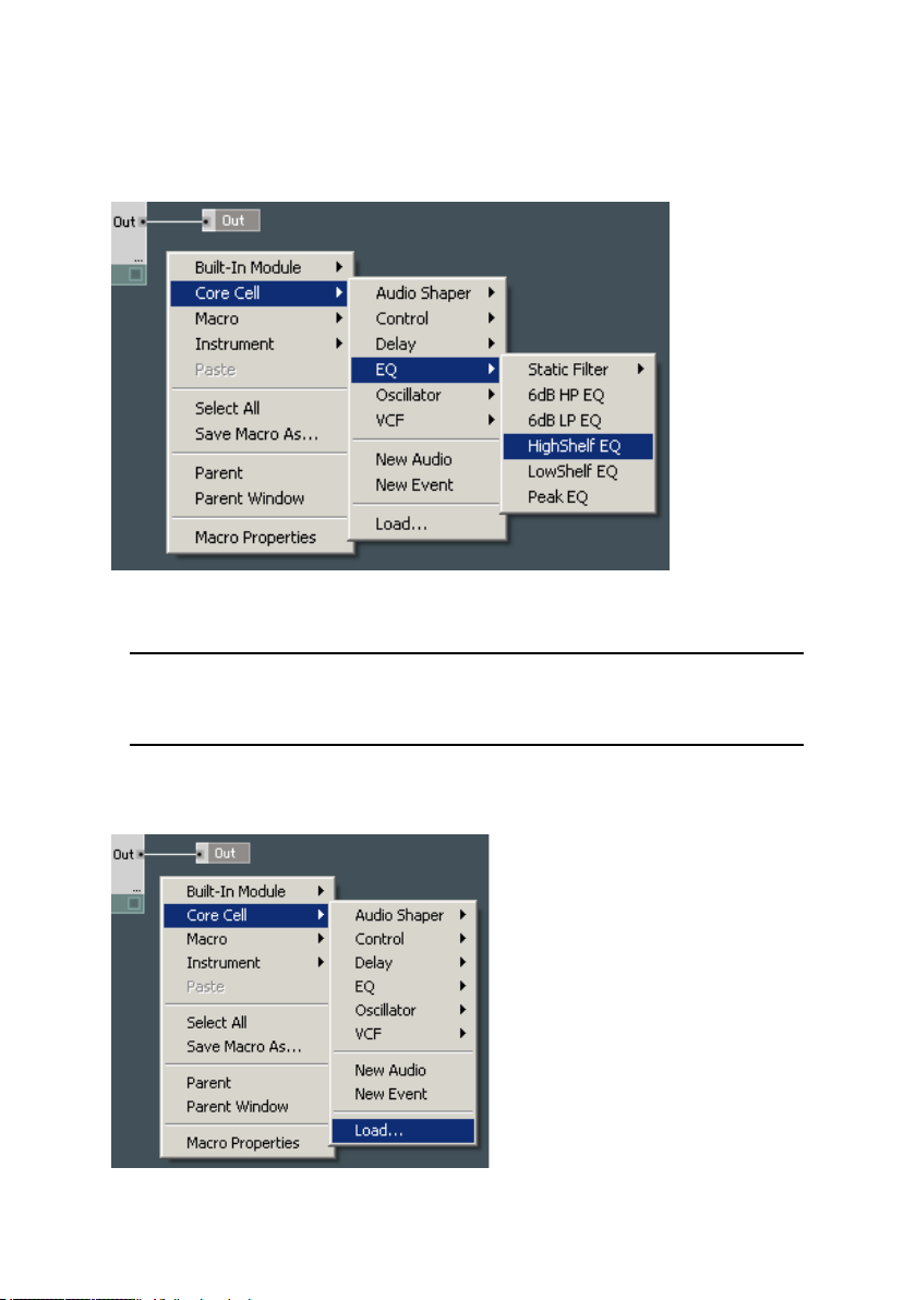
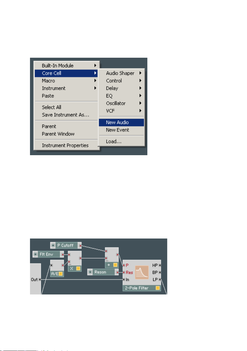
1.2. Using core cells

The core cell library can be accessed from primary-level structures by rightclicking on the background and using the Core Cell submenu:

As you can see, there are all different kinds of core cells; they can be used in the same way as primary-level built-in modules.

An important limitation of core cells is that you are not allowed to use them inside event loops. Any event loop occurring through a core cell will be blocked by Reaktor.

You can also insert core cells that are not in the library. To do that, use the Load… command from the Core Cell menu:

12 – REAKTOR CORE

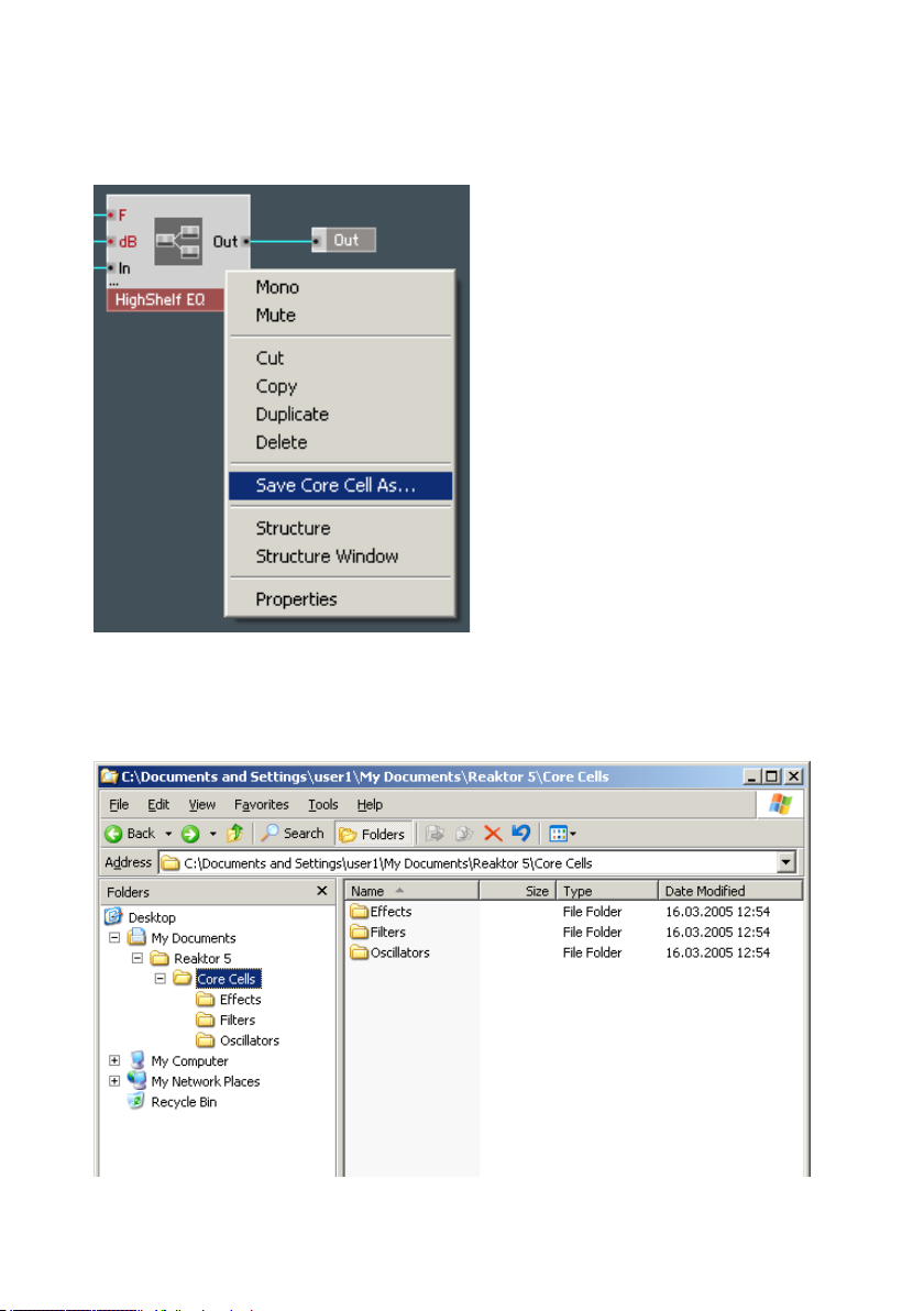
You may also want to save core cells you’ve created or modiﬁed, so that you can load them into other structures. To save a core cell, right-click on it and select Save Core Cell As:

Rather than using the Load… command, you can have your core cells ap- pear in the menu by putting them into the Core Cells subdirectory of your user library folder. Better still, you can further organize them into subgroups. Here’s an example:

REAKTOR CORE – 13

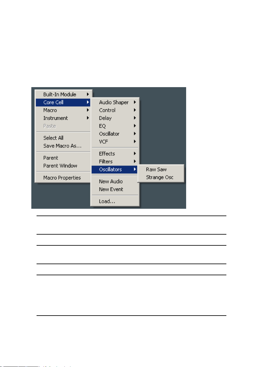
“My Documents\Reaktor 5” is the user library folder in this example. On your computer there may be a different path, depending on the choice you’ve made during installation and any changes you’ve made in Reaktor’s preferences. Inside the user library folder there’s a folder named “Core Cells”. (Create it manually if it doesn’t exist.) Inside the Core Cells folder, notice the folder structure consisting of the Ef- fects, Filters, and Oscillators folders. Inside those folders are core cell ﬁles that will be displayed in the user part of the Core Cell menu:

The menu contents are scanned once during Reaktor startup, so after putting new ﬁles into these folders, you should restart Reaktor.

Empty folders are not displayed in the menu; a folder must contain some ﬁles to be displayed.

Under no circumstances should you put your own ﬁles into the system library. The system library may be changed or even completely replaced when installing updates, in which case your ﬁles will be lost. The user library is the right place for any content that is not included in the software itself.

14 – REAKTOR CORE

1.3. Using core cells in a real example

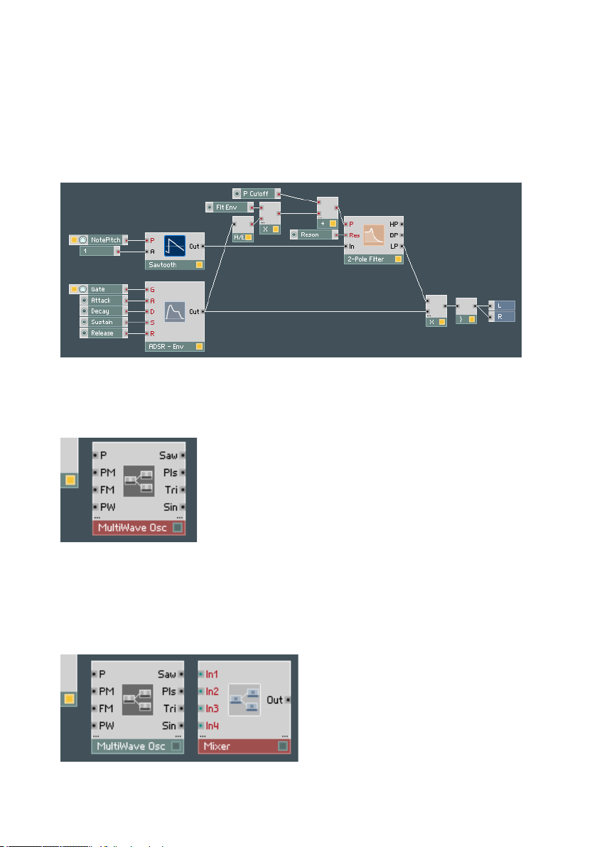
Here we are going to take a Reaktor instrument built using only primary-level modules and modify it by putting in a few core cells. In the Core Tutorial Examples folder in your Reaktor installation, ﬁnd the One Osc.ens ensemble and open it. This ensemble consists of only one instrument, which has the internal structure shown:

As you can see this is a very simple subtractive synthesizer consisting of one oscillator, one ﬁlter and one envelope. We are going to replace the oscillator with a different, more powerful one. Right-click on the background and select Core Cell > Oscillator > MultiWave Osc:

The most important feature of this oscillator is that it simultaneously provides different analog waveforms that are locked in phase. We are going to replace the Sawtooth oscillator with the MultiWave Osc and use a mix of its waveforms instead of a single sawtooth waveform. Fortunately, there’s already a mixer macro available from Insert Macro > Classic Modular > 02 - Mixer Amp > Mixer – Simple – Mono:

REAKTOR CORE – 15

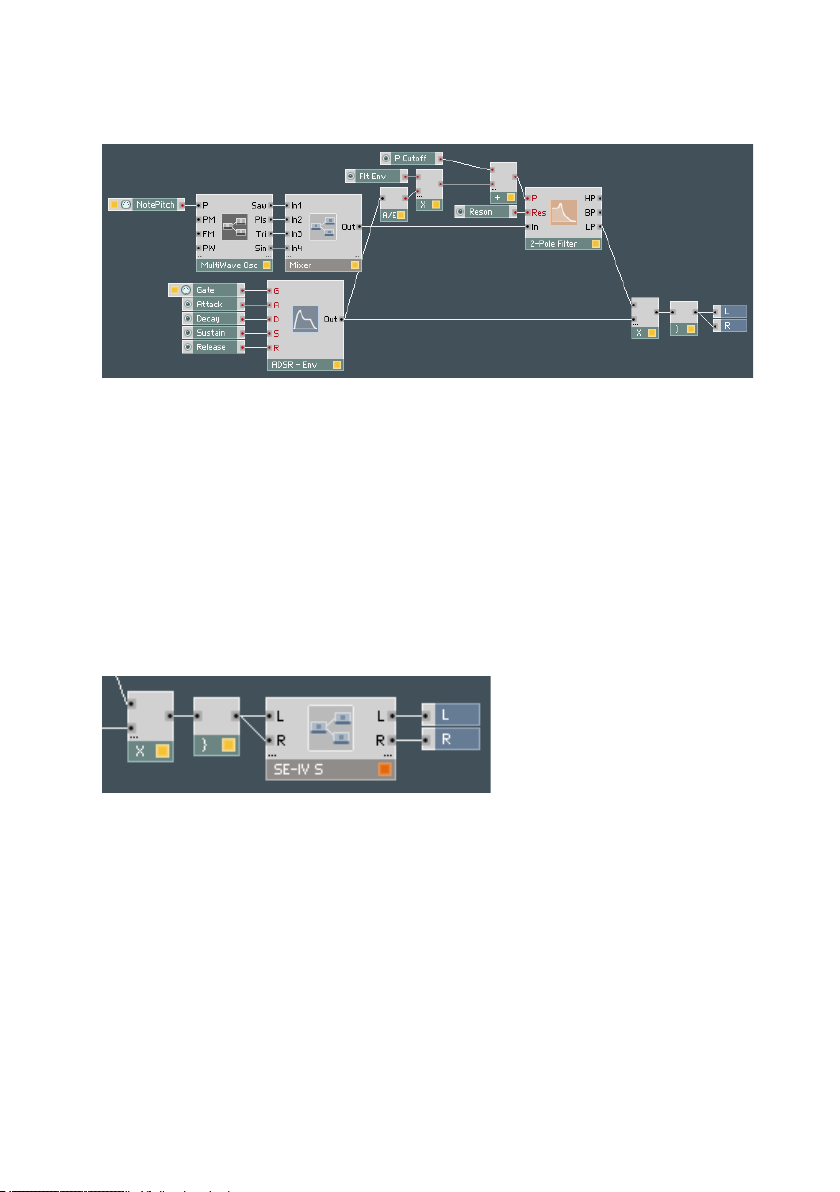
Connect the mixer and the oscillator together and use their combination to replace the sawtooth oscillator:

Switch to the panel view. Now you can use the four faders of the mixer to vary the waveform mix. Let’s do one more modiﬁcation to the instrument and add a Reaktor Core-based chorus effect. We say Reaktor Core based, because although the chorus itself is built as a core cell, the part containing panel controls for this chorus is still built using the primary-level features. That’s because at this time Reaktor Core structures cannot have their own control panels – the panels have to be built on the primary level.

Select Insert Macro > Building Blocks > Effects > SE-IV Chorus and insert it after the Voice Combiner module:

If you look inside the chorus you can see the chorus core cell and the panel controls:

16 – REAKTOR CORE

1.4. Basic editing of core cells

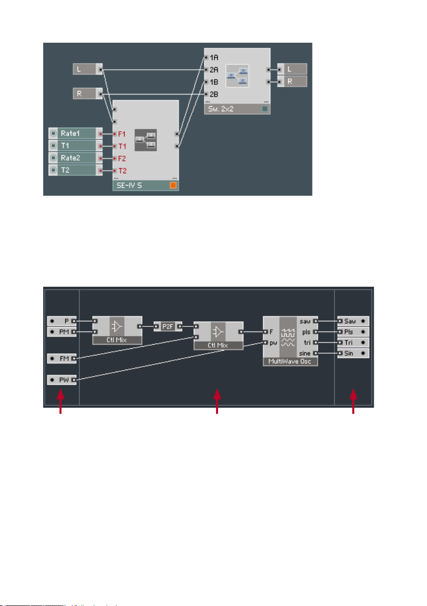
Now we are about to learn a few things about editing core cells. We are going to start with something simple: modifying an existing core cell to your particular needs. First, double-click the MultiWave Osc to go inside:

Inputs Normal Outputs

What you see now is a Reaktor Core structure. The three areas separated by vertical lines are for three different kinds of modules: inputs (on the left), outputs (on the right), and normal modules (center). Whereas normal modules can move in all directions, the inputs and outputs can only be moved vertically, and their relative order matches the order in which they appear outside. So, you can easily rearrange their outside order by moving them around. Try moving the FM input below the PW input:

REAKTOR CORE – 17

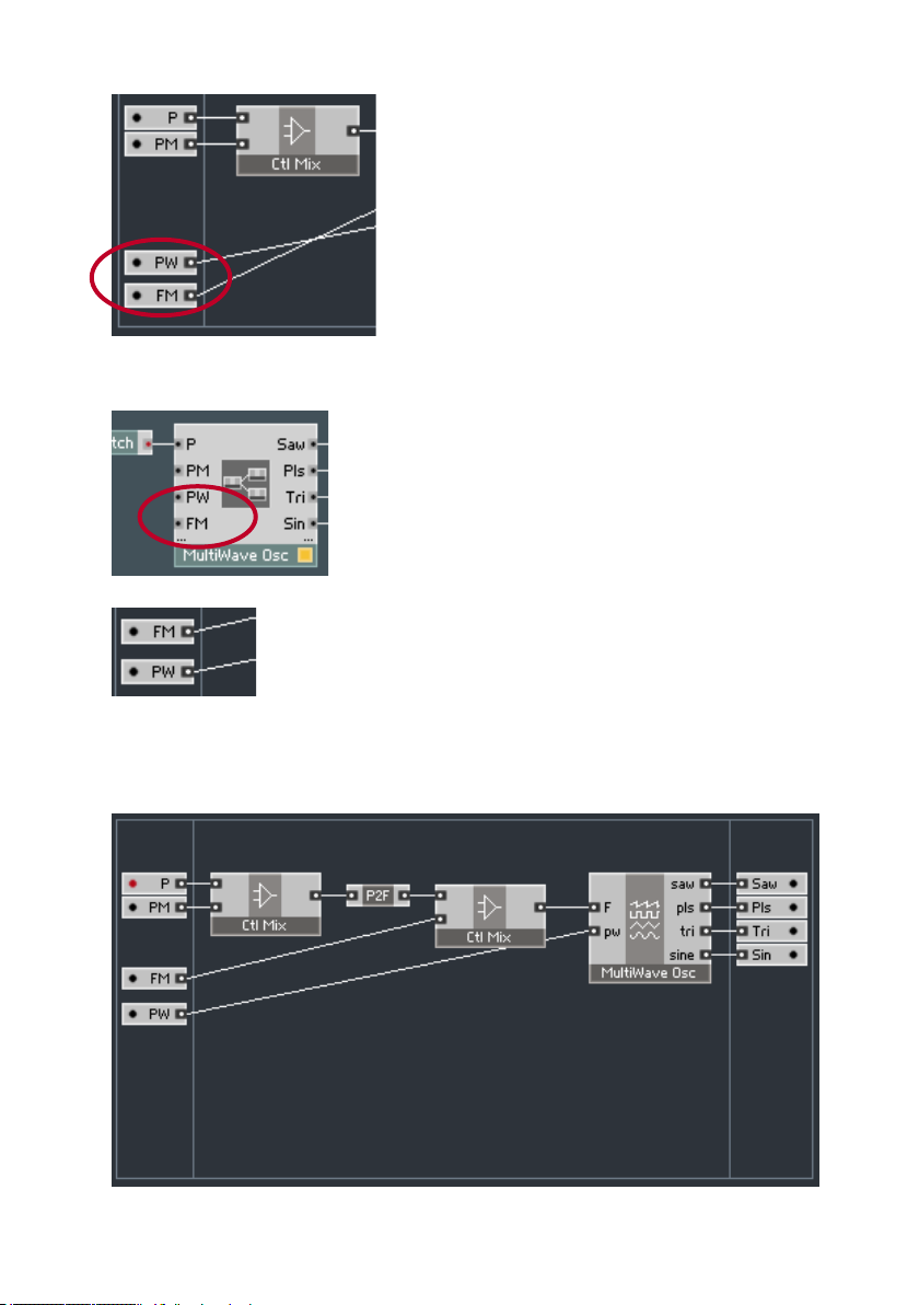
You can double-click the background now to ascend to the outside, primarylevel structure and see the changed port order:

Now go back to the core level and restore the original port order:

As you have probably already noticed, if you move modules around, the three areas of the core structure automatically grow to accommodate all modules inside them. However, they do not automatically shrink, which can lead to these areas sometimes becoming unnecessarily large:

18 – REAKTOR CORE

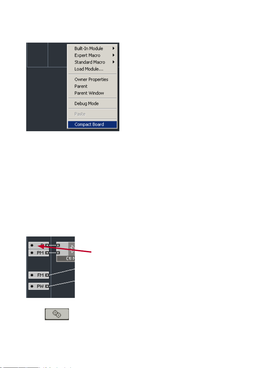
You can shrink them back by right-clicking on the background and selecting Compact Board command:

Now that we have learned to move the things around and rearrange the port order of a core cell, let’s try a few more options. For a core cell that has audio outputs it’s possible to switch the type of its inputs between audio and event (a more detailed explanation can be found later in this manual). In the above example, we used a MultiWave Osc module, all of whose inputs and outputs are audio. However, in this example we don’t really need them as audio, because the only thing connected to the oscillator is a pitch knob. Wouldn’t it be more CPU efﬁcient to have at least some of the ports set to event type? The obvious answer is, “yes, it would.” Here’s how to do that. Changing both P and PM inputs to event mode should produce the largest CPU improvement. To do that double-click on the P port module to open its properties window:

Double-click here

Switch the properties window to the function page, if necessary, by clicking

on the tab. You should now see the Signal Mode property:

REAKTOR CORE – 19

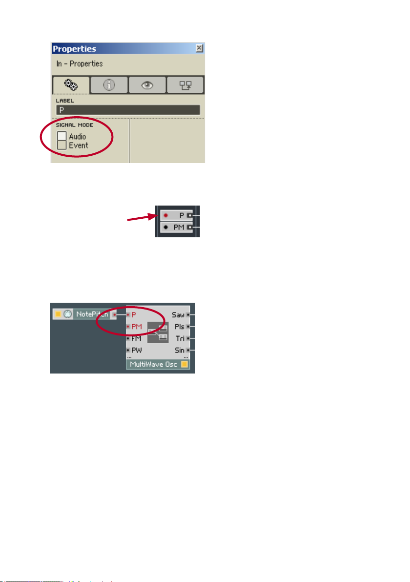
Change it to event. Note how the large dot at the left of the input module changes from black to red indicating that the input is now in event mode (it’s more easily visible after you deselect the port – just click elsewhere):

The dot turns red

Now click on the PM input to select it, and change it to event mode, too. If you want, you can change the two remaining inputs to event mode as well. Finally, double-click the structure background to return to the primary level and observe that the port colors have changed to red and the CPU usage has gone down.

Sometimes it doesn’t make sense to switch a port from one type to another. For example, it doesn’t make sense to switch an input that receives a real audio signal (meaning real audio, not just an audio-rate control signal like an envelope) to an event rate. In some cases such switching could even ruin the functionality of the module. Going in the other direction, it doesn’t make sense to change an event input that is really event sensitive, such as an envelope’s event trigger input (for example, gate inputs of Reaktor primary-level envelopes). If you change such an input to audio, it will no longer work correctly. In addition to cases in which port-type switching obviously does not make sense there may be cases in which it does make sense, but in which the modules will not work correctly if you switch their port types. Such cases are quite special, although they can also result from mistakes in the implementation

20 – REAKTOR CORE

or design of the module. Generally, port-type switching should work; hence the following switching rule:

In a well designed core cell, an audio-rate control input can typically be switched to event mode without any problem. An event input can be switched to audio only if it doesn’t have a trigger (or other eventsensitive) function.

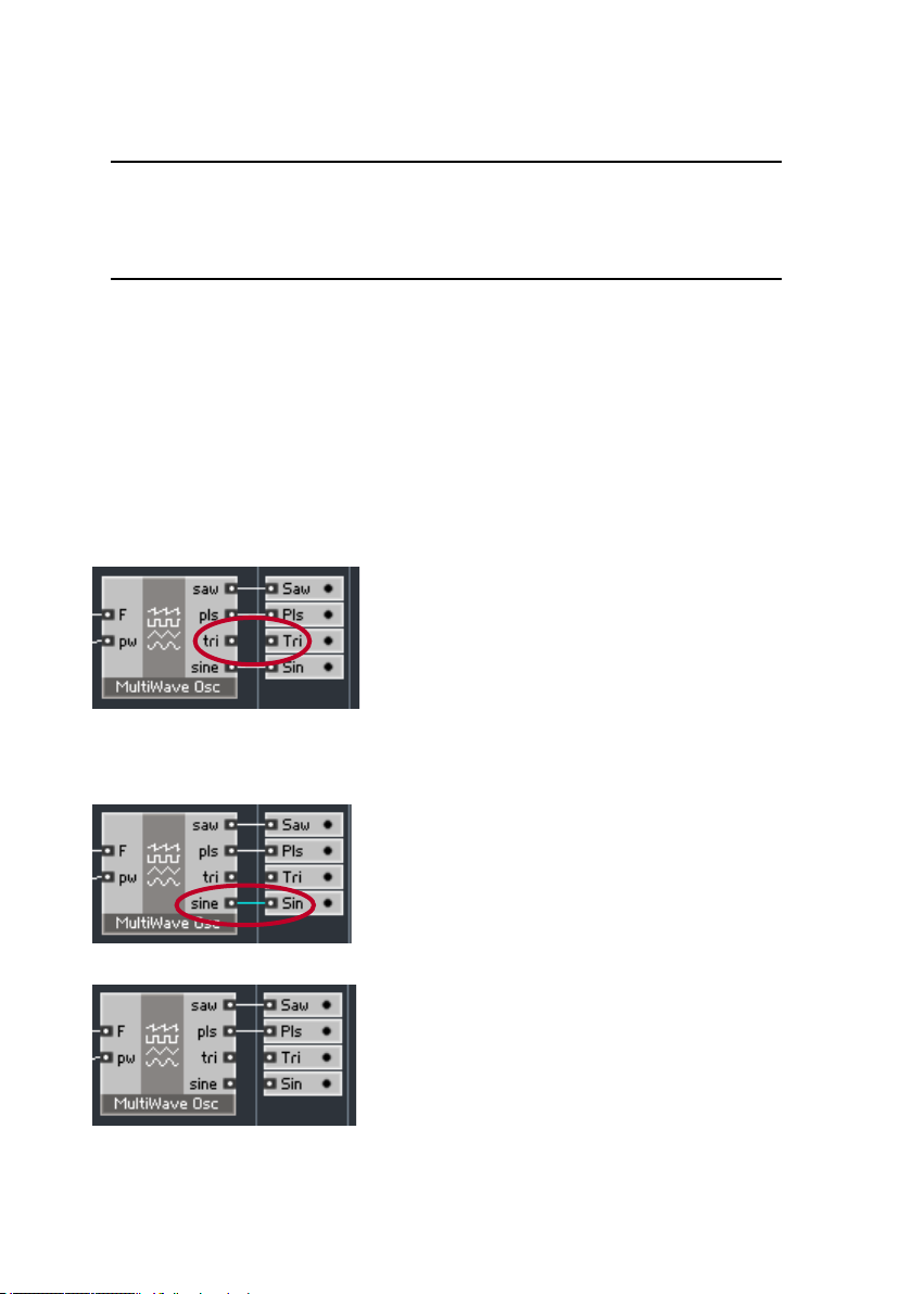
Another way to save CPU is to disconnect the outputs that you don’t need, thereby deactivating unused parts of the Reaktor Core structure. You have to do that from inside the structure – outside connections do not have any effect on deactivating the core structure elements. Suppose in our example we decide that we only need the sawtooth and pulse outputs. We can lower the CPU usage by going inside the MultiWave Osc and disconnecting the unused outputs. Disconnecting is simple in Reaktor Core, you click on the input port of the connection, drag the mouse to the any empty part of the background and release it. For example, click on the input port of the Tri output and drag the mouse into empty space on the background.

There’s another way to delete a connection. Click on the wire between the sine output of the MultiWave Osc and Sin output of the core cell, so that it gets selected (you can tell that it’s selected by its blue color):

Now you can press the Delete key to delete the wire:

After you deleted both wires, the CPU meter should go down a little more.

REAKTOR CORE – 21

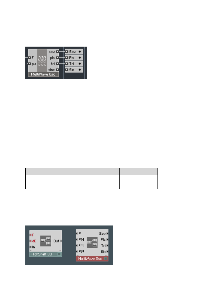
If you change your mind, you can reactivate the outputs by clicking on either the input or the output that you want to reconnect and dragging the mouse to the other port. For example, click on the Tri output of the MultiWave Osc and drag to the input of the Tri output module. The connection is back:

Of course, numerous ﬁne-tuning adjustments can be made to core cells. You will learn about many more options as you proceed through this manual.

2. Getting into Reaktor Core

2.1. Event and audio core cells

Core cells exist in two ﬂavors: Event and Audio. Event core cells can receive only primary-level event signals at their inputs and produce only primary-level event signals at their outputs in response to such input events. Audio core cells can receive both event and audio signals at their inputs but provide only audio outputs:

Flavor Inputs Outputs Clock Src

Event Event Event Disabled

Audio Event/Audio Audio Enabled

Therefore audio cells can implement oscillators, ﬁlters, envelopes, effects and other stuff, while event cells are suitable only for event processing tasks. The HighShelf EQ and MultiWave Osc modules that you are already familiar with are examples of audio core cells (you can tell that by the fact that they have audio outputs):

22 – REAKTOR CORE

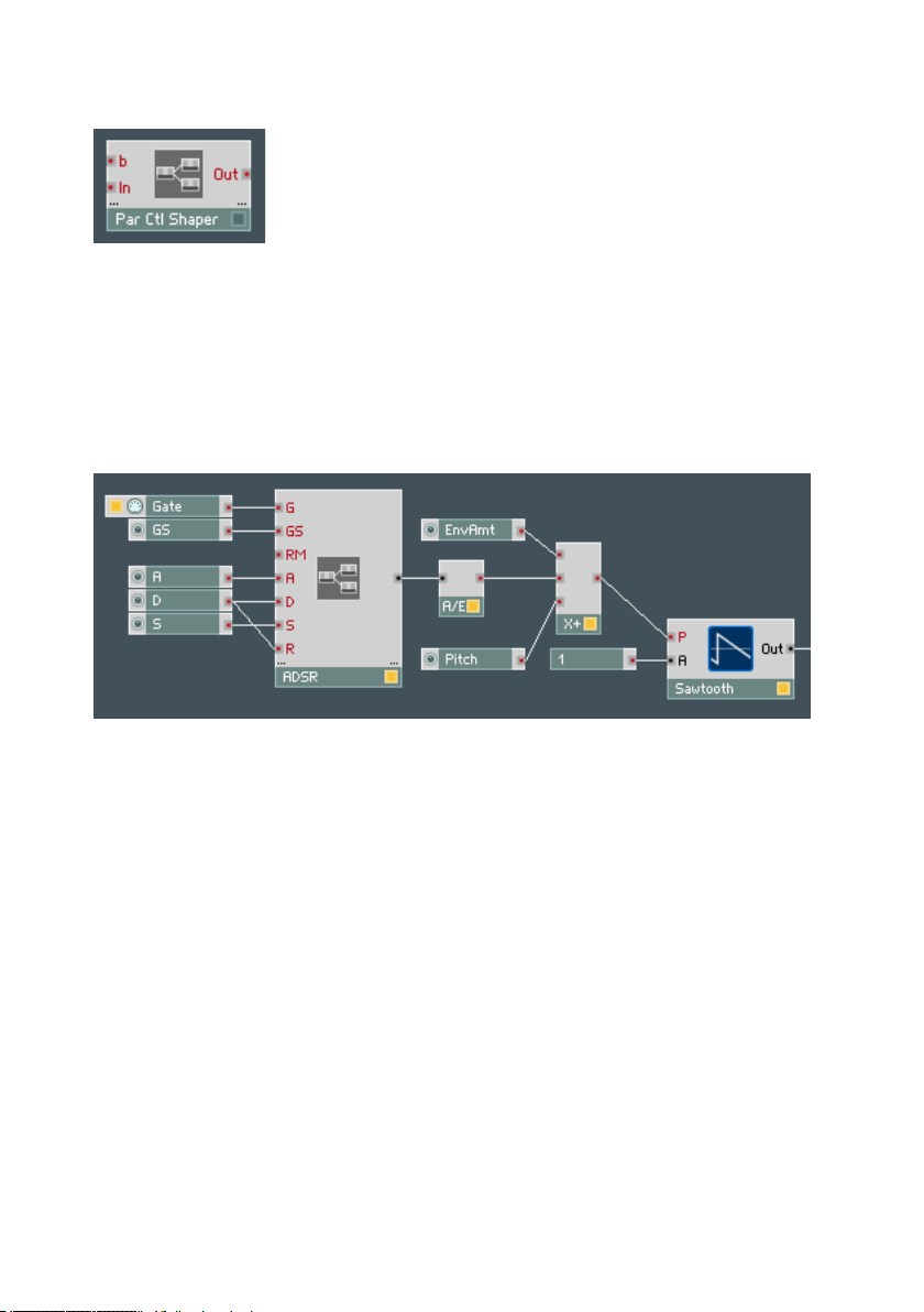
And here is an example of an event core cell:

This module is a parabolic shaper for control signals, which can be used to implement velocity curves or LFO signal shaping, for example. As previously mentioned, event core cells are restricted to event processing tasks. Because clock sources are disabled inside them (see the table above), they cannot generate their own events and, therefore, cannot implement modules such as event-rate LFOs and envelopes. When you need such modules, we suggest that you take an audio cell and convert its output to event rate using one of the primary-level audio to event converters:

The above structure uses an audio core cell implementing an ADSR envelope and converts it to event rate to modulate an oscillator.

REAKTOR CORE – 23

2.2. Creating your ﬁrst core cell

You create new core cells by right-clicking on the background in a primary-level structure and selecting Core Cell > New Audio or, for event cells, Core Cell > New Event:

We are going to build a new core cell from scratch inside the same One Osc.ens you already played with. We will be using the modiﬁed version of that ensemble with the new oscillator and chorus that we built in the last chapter, but if you didn’t save it don’t worry, you can do the same steps using the original One Osc.ens. As you can see, in this ensemble we are modulating the ﬁlter at the P input, which accepts only event signals. We are not using the FM version of the same ﬁlter because it does not perform as well at higher cutoff frequencies, and because the modulation scale is linear at an FM input, which generally gives less musical results when modulated by an envelope. (That phenomenon is typically but incorrectly referred to as “slow envelopes”.):

Because we need to apply the modulation at an event input, we also need to convert the envelope’s output to an event signal, which we do with an A/E

24 – REAKTOR CORE

converter. As a result, our control rate is pretty low. Of course we could have used a converter running at a signiﬁcantly higher rate (and eating up signiﬁcantly more CPU), but what we are going to do instead is replace this ﬁlter with one which we build as a core cell. Alternatively, we could have taken an existing ﬁlter from the core-cell library, but then we would miss all the fun of making our ﬁrst Reaktor Core structure. 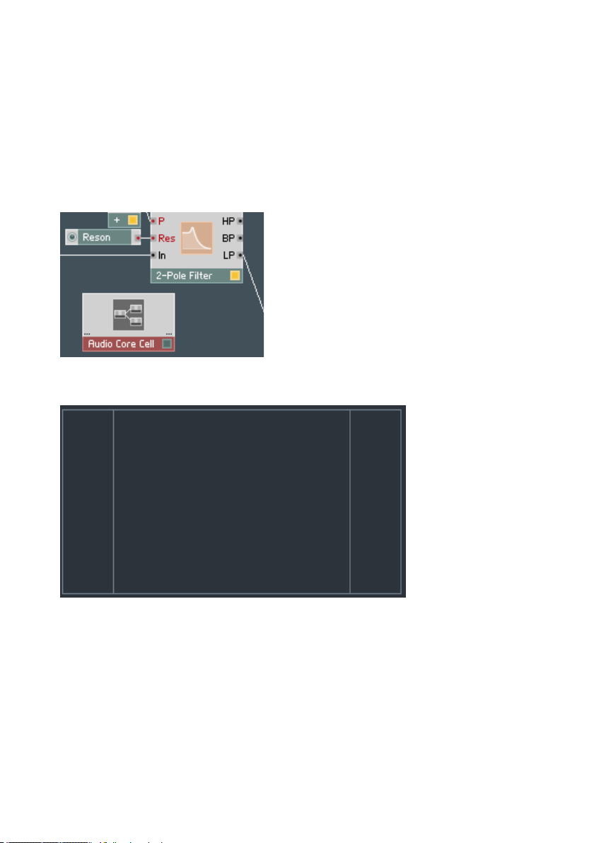We’ll start by creating a new audio core cell. Select Core Cell > New Audio and an empty audio core cell will appear:

Double-click it to see its structure, which is obviously empty. As you surely remember, the three areas are meant for input, output, and normal modules:

REAKTOR CORE – 25

Attention: we are going to insert our ﬁrst module into a core structure right now! Right-click in the normal area to bring up the module creation menu:

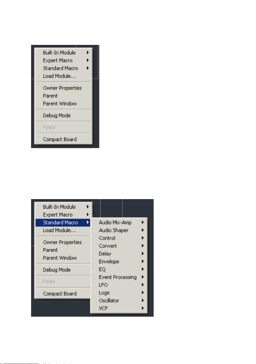
The ﬁrst submenu is called Built-In Module and provides access to the built- in modules of Reaktor Core, which are generally meant to do really low-level stuff and will be discussed later. The second submenu is called Expert Macro and contains macros meant to be used alongside built-in modules for low-level stuff. The third submenu, called Standard Macro, is the one we want to use:

26 – REAKTOR CORE

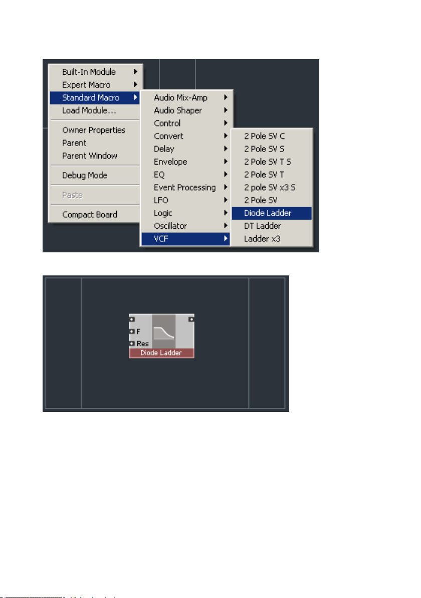
The VCF section could be promising, let’s look inside:

Let’s try Diode Ladder:

Well, maybe that was not the best idea, because a diode ladder might sound signiﬁcantly different from the primary-level ﬁlter module we are trying to replace. At minimum, Diode Ladder is a 4-pole (24dB/octave) ﬁlter, and the one we are replacing is a 2-pole ﬁlter (12dB/octave). To delete it there are two options. One is to right-click on the module and select Delete Module:

REAKTOR CORE – 27

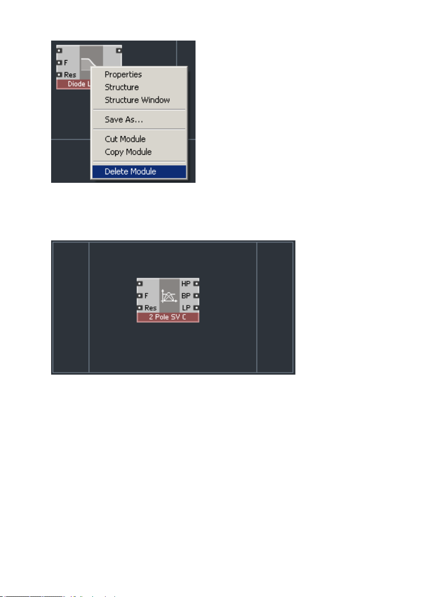
The other option is to select the module by clicking on it and pressing the Delete key. After deleting the Diode Ladder, insert a 2 Pole SV C ﬁlter from the same VCF section of the Standard Macro submenu:

This is a 2-pole, state-variable ﬁlter and is similar to the one we are replacing (there are some differences, but they are quite subtle). What’s important is that we can modulate this ﬁlter at audio rates. Obviously, we need some inputs and some outputs for our core cell. To be exact we need only one output – for the LP signal. To create it right-click in the outputs area:

28 – REAKTOR CORE

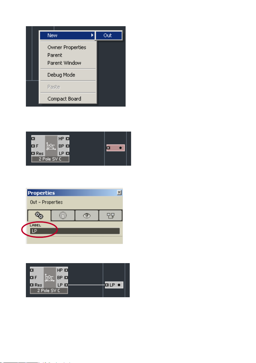
There’s only one kind of module you can create there, so select it. This is what the structure is going to look like:

Double-click the output module to open the Properties window (if it’s not already open). Type “LP” in the label ﬁeld:

Now connect the LP output of the ﬁlter to the output module:

Now let’s start with the inputs. The ﬁrst input will be an audio-signal input. Right-click in the background of the inputs area and select New > In:

REAKTOR CORE – 29

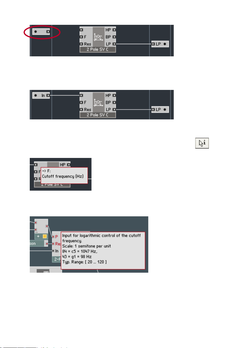
The input is automatically created with the right type – it’s an audio input, as you can tell by the large black dot. Rename this input to “In” in the same way you renamed the output to “LP”, then connect it to the ﬁrst input of the ﬁlter module:

The second input is a little bit more complicated. As you can see, the second input of the ﬁlter Reaktor Core module is labeled “F”. That means frequency,

and if you hold your mouse over that input for a while (make sure the button is active), you’ll see the info text, which says “Cutoff frequency (Hz)”:

As we know, the cutoff of our primary-level ﬁlter module is controlled by an input labeled “P”, and as you can see from the info text, the signal uses a semitone scale.

We obviously need to convert from semitones to Hz. We can do that either on the primary level (using the Expon. (F) module) or inside our Reaktor Core structure. Because we are learning to build Reaktor Core structures, let’s go for the latter option. Right-click in the background of the normal area and select Standard Macro > Convert > P2F:

30 – REAKTOR CORE

As the name implies (and the info text states), this module converts between P (pitch) and F (frequency) scales – exactly what we need. So let’s create a second input labeled “P” and connect it using the P2F module:

That should do it, but wait! In our instrument we have a “P Cutoff” knob deﬁning the base cutoff of the ﬁlter, and to that is added the modulation signal from the envelope, which we have to convert to an event signal on the primary level in order to feed it into the P input of the ﬁlter. Now that the conversion is no longer necessary, we can remove the A/E module and plug the audio signal directly into the audio P input of our new ﬁlter. Although this approach is ﬁne, let’s look at another way, just for fun. We’ll start with our P input in event mode and add another modulation input in audio mode. (If you remember our discussion about slow envelopes, you will understand why we decided to call this input “PM”, not “FM”.) We also need to have the modulation input use the semitones (pitch) scale. That’s exactly how it was done in our original instrument: we added our envelope signal to the “P Cutoff” signal and plugged the sum into the P input. So ﬁrst change the P input to the event mode (as described previously) and add another PM input, which should be in audio mode:

As a user of the Reaktor primary level, you probably expect us to add the two signals together now. In fact, we could do that, but in Reaktor Core the Add is considered a low-level module, and using it generally requires some knowledge of fundamental Reaktor Core low-level working principles. They are not that complex and will be described later in this text. For now, you don’t need to know them; just use a control signal mixer instead, for example, Standard Macro > Control > Ctl Mix:

REAKTOR CORE – 31

The last input that we need is a resonance input, it doesn’t need to be at audio rate, so let’s use an event input:

One other thing we need to do is to give our core cell a name. If the Properties window is already open, click on the background to display the core cell’s properties. If it’s not open, right-click on the background and select the Owner Properties command:

32 – REAKTOR CORE

Now you can type some text into the label ﬁeld:

Double-click the background to see your result:

Wow, looks nice except that the audio-signal input is at the top of the core cell, while the primary-level ﬁlter module input is on the bottom. We could leave it as is, but it’s easy to ﬁx, and you already know how. Let’s do it together, and we’ll show you a new feature on the way. The ﬁrst thing to do is go back inside and drag the audio-signal input all the way to the bottom:

That does the trick, but that diagonal wire over the whole structure doesn’t look particularly nice. That’s what we are going to ﬁx now. Right-click on the output of the In input module and select the Con- nect to New QuickBus command:

REAKTOR CORE – 33

This is what you should see now:

Also, the Properties window should open to display the properties of the QuickBus you’ve just created. The most useful QuickBus property is the ability to change its name (other properties are quite advanced, so don’t touch them for now). You can open the Properties window later by double-clicking on the QuickBus. Although you can rename this QuickBus, we believe the current name is perfect, because it matches the name of the input connected to the QuickBus. (QuickBusses are local to the given structure, so you don’t need to worry about possible name conﬂicts when a neighboring or nested structure is using a QuickBus with the same name.) The next thing you should do is right-click on the top input of the 2 Pole SV C ﬁlter module and select Connect to QuickBus > In:

In the above menu “In” is the name of the QuickBus you are connecting to. You don’t want to create a new QuickBus, you want to connect to one that already exists, and that’s what you’re doing. This is how your structure should look now:

34 – REAKTOR CORE

Instead of a nasty looking diagonal wire, we get two nice references, stating that the input and output are connected by a QuickBus whose name is “In”. Now we can go back out to the primary level and modify our structure to use the new ﬁlter we’ve just built. The Add and A/E modules can be thrown away. This is our ﬁnal result:

Takes quite a bit more CPU, doesn’t it? Well, don’t forget that this ﬁlter is modulated at audio rate in pitch scale. If you don’t like it, you can still revert to the old structure or use the Multi 2-pole FM ﬁlter module from the primary level (slow envelopes, remember?), but we hope that you do like it. Even if you don’t, there are quite a few other ﬁlters with new features that you might like better. And, if you don’t like the new Reaktor Core ﬁlters, there are a whole bunch of other Reaktor Core modules you can try.

REAKTOR CORE – 35

2.3. Audio and control signals

Before we proceed we need to take a look at one particular convention used in the Standard Macros of the Reaktor Core library. The modules you ﬁnd in that area are best described in terms of several different types of signals: audio, control, event, and logic. We will explain event and logic signals a little bit later; for now we’ll concentrate on the ﬁrst two types. Audio signals are obviously signals which carry audio information. These include signals taken at the outputs of oscillators, ﬁlters, ampliﬁers, delays, and so on. Furthermore, modules such as ﬁlters, ampliﬁers, saturators, delays and the like would normally receive an incoming audio signal to process. Control signals, on the other hand, do not carry audio, they are used to control other modules. For example, outputs of envelopes and LFOs as well as keyboard pitch and velocity signals do not carry any sound, but can be used to control a ﬁlter’s cutoff or resonance, or a delay line’s delay time, and so on. Correspondingly, a ﬁlter’s cutoff or resonance input port, or a delay’s time input port are intended to receive control signals. Here is an example of a Reaktor Core ﬁlter module which you already know:

The upper input of the ﬁlter is for the audio signal to be ﬁltered and, therefore, expects an audio-type signal. The F and Res inputs are obviously control type. The outputs of the ﬁlter carry different kinds of ﬁltered audio, so all those signals are also audio type. A sine oscillator module, on the other hand, has only a single control input (for the frequency), and a single audio output:

And if we take a look at the Rect LFO module, it has two control inputs – for controlling the frequency and pulse width (the third input is of event type) – and one control output (because it would be used to control things like ﬁlter cutoff or VCA levels, and so on):

36 – REAKTOR CORE

Some types of processing, mixing for example, make sense for both audio and control types of signals. In those cases, you will ﬁnd versions of such macros dedicated to processing audio and versions dedicated to processing control signals. For example, there are audio mixers and control mixers, audio ampliﬁers and control ampliﬁers, and so on. Generally it’s not a very good idea to misuse a module to process signals of types it was not intended for, unless you really know what you’re doing.

Having said that, quite often it’s possible to use audio signals for control purposes. The most common example would be to modulate an oscillator’s frequency or a ﬁlter’s cutoff by an audio signal. That is absolutely OK because you are intending to use an audio signal as a control signal. We assume that the opposite case, in which you really mean to use a control signal as an audio signal, would be pretty rare.

The separation between audio, control, event, and logic signals is not to be confused with event/audio separation on the Reaktor primary level. The primary-level event/audio classiﬁcation refers to speed of processing, audio signals being processed faster and requiring more CPU. Also as you probably know, primary-level event signals have different propagation rules than audio signals. The difference between audio, control, and event signals in Reaktor Core terminology is purely semantic, deﬁning the meaning of the signal rather than the type of processing. There is not a one-to-one relationship between primary-level event/audio and Reaktor Core audio/control/event/logic terms, but we can still try to explain their relationship:

- a primary-level audio signal normally corresponds to either a Reaktor Core audio signal (for example, an output of an oscillator or an audio ﬁlter) or a Reaktor Core control signal (for example, an output of an envelope).

- a primary-level event signal is typically a control signal in terms of Reaktor Core. An example of such signal would be an output of an LFO, a knob, or a MIDI pitch or velocity source.

- sometimes a primary-level event signal corresponds to a Reaktor Core event signal. The most typical example of that is a MIDI gate (Reaktor Core event signals will be described later, as we promised).

- sometimes a primary event signal resembles a Reaktor Core logic signal; however, they are not fully compatible, and there must be explicit conversion between them (a topic that also will be covered later). Examples include signals processed by Logic AND or similar primary-level modules.

REAKTOR CORE – 37

It’s important to understand that when you select the type for a corecell input port, you are choosing between the primary-level event and audio signals, not between Reaktor Core event and audio signals. The core-cell ports are the place where both worlds meet, and therefore, they use a bit of the primary-level terminology.

We are going to learn a little bit more about this concept while trying to build a tape-echo-effect emulation. We will start by building a simple digital echo, then enhance it to emulate some features of a tape echo. Start by creating an empty audio core cell; then go inside and set its name to “Echo”. The ﬁrst module we are going to put into the structure is a delay module. We will pick a 4-point interpolating delay, because it has better quality than a 2point delay, and a non-interpolating delay would not be suitable for our tape emulation: Standard Macro > Delay > Delay 4p:

We obviously need an audio input and an audio output for our delay core cell. We will use a QuickBus connection for the input and a normal connection for the output:

We also need an event input for controlling the delay time. One thing to be aware of here is that, on the primary level, the delay time is usually expressed in milliseconds, while Reaktor Core library delay macros expect it to be in seconds. No problem, there is a conversion module available for that. Standard Macro > Convert > ms2sec:

So far, we only have a single echo, and it would also be nice to hear the original signal, not just the echo. To get the original signal at the output we need to

38 – REAKTOR CORE

mix it with the delayed signal. Because we are mixing audio signals here, we need to use an audio mixer (you may remember we used a control mixer to mix control signals when we were building a ﬁlter core cell). Even better, we can use a particular audio mixer type that is speciﬁcally designed to crossfade between two signals: Standard Macro > Audio Mix-Amp > XFade (par):

Here “(par)” stands for parabolic, which produces a more natural sounding crossfade than a linear crossfade. We will connect the control (x) input of the crossfade to a new event input to control the mix between the dry (unprocessed) and wet (delayed) signals. When the control signal is 0 we will hear only the original signal, and when it’s 1, we will hear only the delayed signal:

Now we can hear the original signal and the echo, but there’s still only one echo. To have multiple echoes we need to feed a fraction of the delayed signal back to the delay input. First we need to attenuate the delayed signal. Following the same guidelines, use an audio ampliﬁer to attenuate an audio signal by choosing Standard Macro > Audio Mix-Amp > Amount.

We use the Amount amp because we want to control the amount of the signal that is fed back. Also, this ampliﬁer will allow us to invert the signal by using negative amount settings. In contrast, for example Amp (dB), which would be quite suitable to control the signal volume, is not very good here because it doesn’t allow us to invert signals. We connect the amplitude control input of the ampliﬁer to an event input controlling the feedback amount:

REAKTOR CORE – 39

The reasonable feedback amount range is something like [-0.9..0.9] here. When you try out this delay, be careful with the feedback amount, because you can easily reach excessive signal levels (there is no saturation in our circuitry yet). We could have embedded a safety feedback amount clipper into our delay core cell, but because we are going to have saturation there a little bit later, we didn’t think that was necessary. Without it, you will be able to experiment with high feedback levels and hear the delay saturating.

We need to mix the feedback signal with the input signal. An audio mixer (Standard Macro > Audio Mix-Amp > Audio Mix) is a natural choice

You may wonder what happened to the upper input of the Amount module above, which now shows a large orange “Z”:

Actually, depending on the version of the software and other conditions, the Z sign could appear at some other input in the structure, but don’t worry you too much about it. The Z sign indicates that a digital feedback has occurred in the structure, and it is meant for advanced structure design, where such information can be an important hint for the structure designer. For simple structures like the one above, one normally needn’t worry about the Z sign; its presence just shows that there will be a 1-sample delay (about

40 – REAKTOR CORE

0.02ms at 44.1kHz, even less at higher sampling rates) at that point in the structure. We assume you won’t notice if your delay time is 0.02ms off the speciﬁed value. Let’s get back to our structure, which now can produce a series of decaying echoes. It is already a decent digital echo, but we want to show you a feature of the library that you can use as a trick to make your structure smaller. Among the audio ampliﬁers are ampliﬁers called “Chain”. These ampliﬁers are capable of amplifying a given signal and mixing it with another, chained signal. One of them is the Audio Mix-Amp > Chain(amount) ampliﬁer, which works similarly to the Amount ampliﬁer except that it also does chained mixing:

The signal at the second input of this module will be attenuated according to the amount given at the A input and mixed with the signal at the chain (>>) input. The signal at the chain input is not attenuated. Such ampliﬁers can be used to build mixing chains, where the >> port connections constitute a mixing bus:

In our case we don’t need a mixing bus, but we can use this module to replace both our Audio Mix and Amount modules. The fed back signal will be attenuated by the amount speciﬁed by the Fbk input and mixed to the input signal exactly as it was before:

Congratulations, you have built a simple digital-echo effect. The next step is to add some tape feel to it.

REAKTOR CORE – 41

2.4. Building your ﬁrst Reaktor Core macros

In the echo effect we just built, we used a Delay 4p macro from the library, which gives us a reasonably high-quality digital delay. But, high-quality or not, it still sounds too digital. We will make it sound warmer by adding two features found in tape delays: saturation and ﬂutter. Let’s start by deleting the delay macro from the structure and creating an empty macro instead. Right-click on the background as select Built-In Module > Macro:

Double-click it to dive inside. You will see an empty structure, similar to the one you are diving from:

It also works similarly, but there are some important differences because the previous one was a structure of a Reaktor Core cell, whereas this one is an internal structure of a Reaktor Core macro. These differences have to do with the available input and output modules, which are different:

42 – REAKTOR CORE

The Latch and Bool C types of ports will be explained much later in this manual and are used for advanced stuff. We are interested now only in the ﬁrst type, which is called “Out” (or “In” for inputs). It’s a general type of port that can accept audio-, control-, event-, and logic-type signals. In fact, the port doesn’t care whether it’s audio, control, event, or logic; the difference is important only for you as a user, because it describes how the signal is to be used; for Reaktor Core they are all the same. There is also no difference between audio/event inputs/outputs as on the previous structure level, because we don’t have Reaktor primary-level signals on the outside any longer, it is pure Reaktor Core now. The ﬁrst thing we are going to do is name the macro, which is done in the same way as for core cells, by right-clicking on the background, selecting Owner Properties, and typing in the name:

The remaining properties of the macro control various aspects of its appearance and its signal processing.

While you are free to experiment with remaining properties as you see ﬁt, we strongly advise against turning the Solid parameter off. We also advise changing the FP Precision sparingly. The meaning of these parameters will be described in the advanced topics of this manual.

The next thing is to create a set of inputs and outputs for our Tape Delay macro:

REAKTOR CORE – 43

The upper input will receive the audio input, and the lower will receive the time parameter. You may have noticed extra ports on the left side of the input modules; we will explain them a little bit later. As the central part of our macro we will use the same Delay 4p module:

A simple emulation of the saturation effect can be done easily by connecting a saturator module before the delay. Saturator is a kind of signal shaper, so we will look for it among the audio shapers (because it is an audio saturator). Standard Macro > Audio Shaper > Parabol Sat:

The input signal will now be saturated within the range of –1..+1. Actually, the range is controlled by the L input of the saturator module, if it is disconnected it defaults to 1. That might be surprising to you because you are probably used to disconnected inputs being treated as if they receive no signal, or put differently, a zero signal. Well, this is not exactly the case in Reaktor Core structures—modules can specify special treatment for disconnected inputs. The saturator, for example, speciﬁes the L input to have a default value of 1. Now we are going to learn to do exactly the same, by specifying a new default value for our T input. Let’s say that if our T input is disconnected we would like it to be treated as if the input value was 0.25 sec. Very easy. Right-click on the port on the left of the T input module and select Connect to New QuickConst. This is what you should see:

In addition, you should have the properties window displaying the properties

of the constant (if it shows a different page, press the tab):

44 – REAKTOR CORE

In the value ﬁeld type a new value of 0.25:

This is how the QuickConst should look now in the structure:

Let’s explain what we have just done. The port on the left side of the input module speciﬁes a so-called default signal. That means that if the input is not connected (on the outside of the macro), the default signal will be taken as the input source. In our case, if the T input of the Tape Delay macro is not connected on the outside, it will behave as if you have connected a constant value of 0.25 to it. Of course, a connection to the QuickConst is not the only possible connection for the default signal input. You can connect it to any other module in the structure, including other input modules. Now that we have saturation and a default value for the T input, let’s emulate a tape ﬂutter effect. A simple way to do that is to modulate the delay time with an LFO. You could experiment with different LFO shapes for better ﬂutter effect, but for now, just take one from the library: Standard Macro > LFO > Par LFO:

REAKTOR CORE – 45

This is a parabolic LFO, which produces a signal similar in shape to a sine, but uses less CPU. Its F input must receive a signal specifying the oscillation rate. We can use a QuickConst again here. A rate of 4 Hz seems reasonable so we can try that:

The Rst input is used for restarting the LFO; we won’t need it for now. Now we need to specify a modulation amount by scaling the output of the LFO. Currently the LFO output signal varies in the range –1 .. 1 and that is way too much. Because we are dealing with control signals here, we are going to use a control amount module, which is similar to the Amount ampliﬁer we used for audio. Standard Macro > Control > Ctl Amount:

A modulation amplitude of 0.0002 should do ﬁne, so we scale the signal to that amount:

Ultimately, we can mix the two control signals (one from the T input and one from the Ctl Amount module) and feed them into the T input of the delay module. The already familiar Ctl Mix module can be used for that:

Actually, we have a Chain type of control mixer that is similar to the mixer we have for audio signals. We could use it to replace the Ctl Amount and the Ctl Mix

46 – REAKTOR CORE

modules in the same way we did earlier in the audio path. Standard Macro > Control > Ctl Chain:

As one last touch for our macro, we are going to change the buffer size for our delay, which deﬁnes the maximum possible delay time. If you hold your

mouse cursor over the Delay 4p macro (and provided the button is ac- tive), you can read in the hint text that the default buffer size corresponds to 1 sec of delay at 44.1kHz:

Let’s increase the amount to 5 seconds (44,100*5 = 220,500 samples). Because each sample requires 4 bytes, we need 220,500*4 = 882,000 bytes, which is almost 1MB). Double-click on the Delay 4p macro:

The module on the left is the delay buffer module. Double-click it (or right-

click and select Show Properties) to edit its properties. Select the tab and you should see the Size property. Change it to 220,500 samples:

REAKTOR CORE – 47

As we have seen, a delay buffer for 5 seconds of audio takes almost 1MB of memory, so be careful when changing delay buffers. That’s most important when the delays are used in polyphonic areas of the structure, because the size of the buffer will be multiplied by the number of voices.

Now we can go outside the Delay 4p macro and then outside the Tape Delay macro we’ve just created (double-click the background) and make the outside connections:

If you haven’t done so yet, try out the echo module now. Here’s a Reaktor primary-level test structure, as simple as possible (note that the Echo module is set to mono):

You might want to enhance it in various ways, for example, by providing knobs controlling the echo parameters, by using a real synthesizer as a signal source, and so on.

48 – REAKTOR CORE

2.5. Using audio as control signal

We have mentioned above that it is possible to use an audio signal as a control signal. As an example of that, we are going to create a Reaktor Core cell implementing a pair of oscillators, in which one modulates the other. Start by creating two multiwave oscillators:

We need pitch control for both of the oscillators, and we are going to listen to the output of the second one, so let’s create the necessary inputs and outputs:

Now we want to take the output of the left oscillator and use it to modulate the frequency of the right oscillator:

The Mod input controls the modulation amount.

REAKTOR CORE – 49

Notice that we are mixing the modulation signal with the P1 input after a P2F converter so the modulation will take place in frequency scale. (It’s also possible to modulate in pitch scale.) It’s also a good idea to scale the modulation amount according to the base oscillation frequency:

If you analyze the above structure from the point of view of control and audio signals you will notice that all of the signals in the structure except the outputs of the oscillators are control signals. The outputs of both oscillators are obviously audio signals. Notice, however, that we are misusing the output of the left oscillator as control signal at the point at which we feed it into the Ctl Chain mixer.

2.6. Event signals

As we said earlier, there are different meanings of the term event signal. You should already be familiar with the idea of Reaktor primary-level event signals. There are several ways of using a primary-level event signal. One is as a control signal (for example, LFO output, knob output, and so on), because it uses less CPU than a primary-level audio signal. In that case, you probably could achieve the same effect with an audio signal. But, there are also cases in which an audio signal won’t work for control, for instance, when you are interested in both the value of the signal and when the value is sent. A primary-level envelope-gate signal is an example of that, because the envelope will be triggered when the event arrives at the gate input. When we were talking about audio, control, event, and logic signals in Reaktor Core we were not really talking about different types of signals (technically they are all the same in Reaktor Core). Rather we are talking about different ways of using a signal. As we now know, a Reaktor primary-level event signal can be used as a control, event, or even logic signal, and as we’ve seen from an earlier example, a Reaktor primary-level audio signal can be used as audio or control. We have already learned to feed primary-level event signals into Reaktor Core structures and use them there as control signals. Event-mode inputs for an audio core cell implementing a ﬁlter that we built earlier is a good example of that. There are also cases in which you would use an event core cell to process

50 – REAKTOR CORE

some primary-level event signals used as control signals. Here’s an example in which an event core cell wraps a control shaper core macro:

The control shaper receives an event rate control signal from the primary level (for example, a MIDI velocity signal, or a primary-level LFO signal), bends it according to the Shp parameter, and forwards the result to the output.

An important restriction of event core cells, which we mentioned earlier, is that all clock sources are disabled inside them. That means that not only oscillators and ﬁlters, but also envelopes and LFOs do not work inside event core cells. Those modules are restricted to receiving events from the primary level of Reaktor, processing them, and sending them back to the primary level, as in the above example.

Alternatively, signals derived from primary-level events can be used as true event signals inside Reaktor Core structures. Let’s take a look at a couple of simple cases of using events inside Reaktor Core. The ﬁrst case is using an envelope in a core structure. As you can guess from the disabled-clock restriction on event core cells, this has to be an audio core cell. So, create a new audio core cell and choose Standard Macro > Envelope > ADSR:

REAKTOR CORE – 51

The top input of the envelope is a gate input, which works similarly to the gate inputs of primary-level envelopes—that is, it opens or closes the envelope in response to incoming events. For that we create an event input for our core cell:

This input will translate the incoming primary-level gate events into the core events. Now let’s take a look at the A, D, S, R inputs. The S (sustain level) input works similarly to the primary level; it expects the incoming signal to be in the 0 to 1 range:

The A, D, R inputs are different, however. Unlike primary-level envelopes they expect time to be speciﬁed in seconds:

That can be solved by using a Standard Macro > Convert > logT2sec, which converts the primary-level envelope times to seconds:

Although all inputs in the above structure are in event mode, the ﬁrst input produces an event signal, whereas the others produce control signals. Our envelope still has two unconnected ports. The GS port sets the gate sensitivity amount. At 0 the envelope completely ignores the gate level and

52 – REAKTOR CORE

is always at full amplitude. At 1 the gate level has maximum effect, as on the Reaktor primary level. We can control this amount from the outside by adding another input:

The RM port speciﬁes the retrigger mode for the envelope:

The look of this port is different from the others because it expects integer values, but that doesn’t mean we cannot connect non-integer signals to this port. We can simply use another event input, and the incoming values will be rounded to the nearest integer:

REAKTOR CORE – 53

Now let’s take a look at another example using a true event signal:

The above structure implements a kind of pitch modulation effect. The effect is produced by a delay whose time varies in the range 250±100 ms. The rate of variation is determined by the Rate input, which controls the rate of the modulating LFO (the value is in Hz)—that is a pure control signal. The Rst input is a true event signal and can be used for restarting the LFO. The incoming value speciﬁes the restart phase, where 0 would restart the LFO at the beginning of the cycle, 0.5 in the middle, and 1 in the end. You can try it out by connecting a button to send a speciﬁc value to this input.

2.7. Logic signals

Now that we have learned about control and event signals, it’s time to learn about another way of using signals in Reaktor Core, that would be as logic signals. Here’s an example of a module that processes logic signals:

Notice that the ports of this module are integer type, just as was the RM input of the envelope. That is because, generally, logic signals carry only integer values; more precisely, they carry only values of 0 and 1. For logic signals, a value of 1 stands for true, and a value of 0 stands for false. The meaning of “true” and “false” is, of course, up to the user; for instance, it could mean (as in the example here) whether a particular gate is open (true) or closed (false):

Here a Gate2L macro checks the incoming gate signal and produces a true (1) output if the gate is open and false (0) output if the gate is closed. We can use logic signals to do logical processing. For example, here we’ve built a gate processor that applies a regular clocked gate over a MIDI gate:

54 – REAKTOR CORE

The Gate2L, AND, and L2Gate modules are logic modules and can be found in Standard Macro > Logic menu. The Gate LFO is a macro, which we’ve built for this processor; it generates an opening and closing gate signal at regular intervals. The input gate and the output of the LFO are connected to Gate2L converters, which convert the gate signals to logic signals, transforming open gates into true and closed gates into false. The AND module outputs a true signal only if both gates are in the open state at the same time. In other words the output of the AND module is true if and only if the user holds a key and at the same time the LFO outputs an open gate. That means that, as long as the user holds a key, there will be alternating true and false values at the output of the AND module, the speed of the alternation deﬁned by the LFO rate. The output of the AND module is converted back to a gate signal, whose amplitude is taken from the gate input, thereby leaving the gate level unchanged. Here is the structure for our Gate LFO macro:

The F input deﬁnes the rate of the gate repetitions, and the W input deﬁnes the duration of open gates (at 0 they are 50% of the gate period, at –1 it’s 0%, and at 1 it’s 100%). The Rst input restarts the LFO in response to incoming events (hence the LFO is restarted each time there’s a gate event at the main gate input). The module connected to the Rst input of the Rect LFO is called Value and can be found in Standard Macro > Event Processing. It ensures the LFO is restarted at zero phase by replacing the values of all incoming events by the value at its lower input, which is zero. The LFO output is converted into a gate signal by using a Ctl2Gate converter, also found in Standard Macro >Event Processing.

Remember, LFOs do not work inside event core cells. If you want to try out this structure, you’ll need to use an audio core cell.

REAKTOR CORE – 55

3. Reaktor Core fundamentals: the core signal model













3.1. Values

Most of the outputs of Reaktor Core modules produce values. (Producing a value means that at any moment in time there is a value associated with the output.) The values are available to all modules whose inputs are connected to those outputs. In the following example an adder module gets values 2 and 3 from the two modules whose outputs are connected to its inputs, and it produces a value of 5 at its output.

If you want to draw an analogy to the hardware world you can think of values as signal levels (voltages), especially with relatively large-scale modules such as oscillators, ﬁlters, envelopes, and so on. However, values are not limited to those kinds of processing—they are just values and can be used to implement any processing algorithm, not just voltage-modeling algorithms.

3.2. Events

Time is not continuous in the digital world; it is discrete. Probably the most familiar example of this is that a digitally stored recording doesn’t store the full information about an audio signal, which is continuously changing over time, but rather stores only information about the signal level at regularly spaced points in time. The number of points per second bears the famous name of sampling rate.

56 – REAKTOR CORE

Here is a picture of a continuous signal:

�





 





 

 



and its digital representation:

Because we are in the digital world, the outputs of our modules cannot change values continuously. On the other hand, we don’t have to limit ourselves to changing values at regularly spaced points in time. For one thing, we do not have to maintain a particular sampling rate all over our structures. For another thing, in certain areas of our structures we do not even have to maintain any sampling rate at all; that is, our changes do not have to happen at regular intervals. For example, at time zero the output of our adder could have a value of 5. The ﬁrst change could occur at time 1 ms (one millisecond). The second change could occur at 4 ms. The third at 6 ms:

REAKTOR CORE – 57

In the picture above we can see changes of the output of our adder occurring

























during the time from 0 to 7 ms. At the moment in time that the output changes its value, it generates an event. An event means that the output reports a change of its state, meaning that it has got a new value. In the following example, the upper left module has changed its output value from 2 to 4, generating an event. In response, the adder module will change its output value and generate an event at its output, too.

Alternatively, the upper left module could have generated a new event with the same value as the old one. The adder would have still responded by generating a new event, but this time, without changing its output value.

The new value appearing at the output is not required to be different from the old one. However, the only way an output can change its value is by generating an event.

As you have seen from the previous examples, an event occurring at an output of some module will be sensed by downstream modules, which would in turn produce further events (remember the adder producing an output event in response to an incoming event). Those new events would be sensed by the modules connected to the corresponding outputs and propagated further downstream, until the propagation stops for one of the reasons discussed later in this text.

Events in Reaktor Core are not the same as events on the Reaktor primary level. They behave according to different rules, which will be explained below.

58 – REAKTOR CORE

3.3. Simultaneous events







 



















Consider the situation in which the two modules on the left side in the previous examples simultaneously produce an event.

This is one of the key features of the Reaktor Core event model—events can occur simultaneously at several places. In that situation, the events originating at both the left-side modules will arrive at the inputs of the adder simultaneously, and most importantly, the adder will produce exactly one output event in response.

That is not the same as on the Reaktor primary level, where events cannot happen simultaneously, and the Add module (in event mode) would produce two output events in such a situation.

Of course, in reality, the events are not produced simultaneously by the upperleft and the lower-left modules, because both modules are being processed by the same CPU, and the CPU can process only one module at a time. But, what is important for us, is that these events are logically simultaneous, that is they are treated as simultaneous by the modules receiving them. Here is another example of simultaneous event propagation:

In the example above, the leftmost module is sending an event, changing its output value from 2 to 3. The event is sent simultaneously to both the inverter (–x) and the multiplier (*) modules. In response to the incoming event the inverter will produce a new output value –3. It is important to notice that although the output event of the inverter was produced in response to the event sent by the leftmost module, and as such should happen later than the

REAKTOR CORE – 59

incoming event, both events are still logically simultaneous. That means they simultaneously arrive at the inputs of the multiplier, and the multiplier again produces only one output event, with a value of –9.

Again, on the primary level you would have had two events at the output of the Event Mult module. It is also not deﬁned whether the event at the output of the leftmost module would have been sent ﬁrst to the inverter or to the multiplier (although that is irrelevant for the given structure).

In general you can use the following rule to ﬁgure out whether two events are simultaneous or not:

All events originating from (sent in response to) the same event are simultaneous. All events originating from an arbitrary number of simultaneous events (occurring at different outputs, but known to be simultaneous) are also simultaneous.

The last example shows the beneﬁt of having simultaneous events. In that case, we eliminate the redundant processing of the second event by the multiplier, which would have taken extra CPU time. In longer structures, in the absence of simultaneous events, the number of events can grow uncontrollably unless the structure designer pays particular attention to keeping the number of duplicate events low. In addition to saving CPU time, the concept of simultaneity leads to important differences in one’s approach to structure construction, especially for the structures implementing low-level DSP algorithms. You will become more familiar with these differences as you start constructing your own structures.

60 – REAKTOR CORE

3.4. Processing order



















As you have seen from the previous examples, when a module sends an event, the downstream modules respond to that event. From that, one might conclude that, despite producing logically simultaneous events, the modules are deﬁnitely not processed simultaneously. One might further conclude that, for a given connection, it would be reasonable to process the upstream module of the connection before the downstream module of the connection. All those conclusions are, in fact, correct. The general rule of processing order of the modules is:

If two connected modules are processing logically simultaneous events, then the upstream module will be processed ﬁrst. If the events are not simultaneous, then of course, the order of processing for the modules is the order of the processed events.

From the above rule it follows that as long as there is a one-direction connection path (always upstream or always downstream) between two modules, then there is a deﬁned processing order for these two modules: the upstream module is processed ﬁrst.

If there is no one-direction connection path between two modules, their processing order relative to each other is undeﬁned for logically simultaneous events. That means that the order is arbitrary and can change as a result of various actions. The structure designer must take care that such situations occur only for modules whose relative processing order is unimportant. That is normally automatically the case as long as no OBC connections (see below) are involved.

Here is an example, the digits showing the order of module processing:

For the above structure, there is an alternative valid processing order:

REAKTOR CORE – 61





















There is no way to tell which one will be taken by the software. Fortunately,



 













as long as you do not use OBC connections, the relative order of modules in such cases is really unimportant.

The above rules for processing order cannot be applied if there is feedback in the structures, because in that case, for any pair of modules in the feedback loop we cannot tell which one is upstream to the other. The problem of handling feedback loops, including the processing order, will be addressed later.

For the above structure, it is not possible to deﬁne whether, for example, module B is upstream to module D or vice versa, because there is an upstream connection going from D to B as well as an upstream connection going from B to D (via E).

3.5. Event core cells reviewed

Let’s take a look at event core cells from the point of view of the just described event concept of Reaktor Core. As you’ll remember, event core cells have event inputs and event outputs. These inputs and outputs are the interface between Reaktor’s primary level and the Reaktor Core level; they perform the conversion between primarylevel events and core events, and vice versa. The rules of the conversion are as follows:

62 – REAKTOR CORE

Event Inputs send core events to the inside of the structure in response





























to primary-level events coming from outside. Because the outside primary-level events cannot arrive simultaneously at the inputs, the internally produced events also do not occur simultaneously.

Event Outputs send primary-level events to the outside of the structure in

response to core events coming from the inside. Although core events can occur simultaneously at several outputs, primary-level events cannot be sent simultaneously. Therefore, for simultaneous core events, the corresponding primary-level events will be sent one after another,

with upper outputs always sending before lower ones.

Let’s try that in practice by building an event processing module that performs signal shaping according to the formula: y = 0.25*x*(4-|x|) The graph of this function looks as follows:

Let’s start by creating a new event core cell with one input and one output, labeled “x” and “y”, respectively.

Now let’s create the structure which computes the formula. We need to create |x| (absolute value), - (subtract), and two * (multiply) modules in the normal area. These are not core macros, but rather true Reaktor Core built-in modules. To insert built-in modules into core structures, right-click in the background of the normal area and select the Built-In Module submenu:

REAKTOR CORE – 63

You’ll ﬁnd all the necessary modules in the Built-In Module > Math sub- menu:

We’ll need two constant values: 0.25 and 4. We could use QuickConsts exactly like we did earlier, but we can also insert real constant modules: Built-In Module > Const (as with the QuickConst, their values can be speciﬁed in the Properties window):

64 – REAKTOR CORE

Of course, in this particular case there is no beneﬁt in using Const modules instead of QuickConsts, but sometimes you might want to. For example, if the same constant has to be connected to multiple inputs, it may be better to use a Const module, because then you need only one of them and you also have a single place to edit the value. The above structure now shapes the signal in the way described, but as we’ll see at the end of this section, the implementation is not perfect. For now, let’s give our module a name and go back to the primary level:

Now let’s test it. Set the number of voices for the Reaktor instrument to 1, so that it will be easier to use a Meter module:

REAKTOR CORE – 65

Create a Knob and a Meter and connect them to the input and output of your module:

Set up the properties for the knob and the meter. Don’t forget to set the meter to display its value:

and to check the Always Active box:

66 – REAKTOR CORE

Now move the knob and watch the output value change.

The event-shaper structure we’ve built should work perfectly for shaping control signals, but it still has one minor ﬂaw in its event-processing behavior. We will return to that problem and ﬁx it a little bit later.

REAKTOR CORE – 67

4. Structures with internal state









4.1. Clock signals

How a Reaktor Core module processes an incoming event is completely up to the module. Normally a module would process the incoming value in some way, but it can also completely ignore it. The most typical case of such processing is clock inputs. One example of a module with a clock input is a Latch. The Latch is not a built-in module; it’s a macro; nevertheless, it’s perfect for demonstrating the clock principle. The Latch has two inputs – one for the value and one for the clock.

The value input (the upper one) will store the incoming value to the internal memory of the latch in response to an incoming event; nothing will be sent to the output. The clock input will send the last stored value to the output in response to an incoming event.

Clock inputs (unless otherwise speciﬁed) completely ignore the value of the incoming event and respond only to the fact that the event is coming.

(Because now we are discussing clock signals, not latches, examples of using the Latch module will come later.) Because there are modules with clock inputs, it should be clear that some of the signals in the structure do not carry any used (or, for that matter, useful) values. Some signals can even be produced for the sole purpose of being used as a clock source. We will call them clock signals. A sampling-rate clock is one example of a clock signal. It produces an event for each new audio sample to be generated, so at 44.1 kHz sampling rate it would tick 44,100 times per second. The value of the signal has no meaning, is not intended to be used in any way, and is (in the current implementation) always zero.

68 – REAKTOR CORE

4.2. Object Bus Connections





















 





 







 





 







Object Bus Connections (OBC) are a special type of connection between modules. An OBC connection between two modules declares that they share some internal object. The most typical case of modules using OBC connections are memory Read and Write modules, which would share a common memory if connected by an OBC. The functionality of the Write module is to write a value that is incoming at its input, to the OBC-shared memory. The functionality of the Read module is to read a value from the OBC-shared memory in response to an incoming clock signal (C input). The read value is sent to the output of the Read module.

The above structure implements the functionality of the Latch macro (in fact, it is the internal structure of the Latch macro). The M and S pins of Read and Write modules are pins of Latch OBC type. The M pin is the master connec- tion input, the S pin is the slave connection output. The master input of the Read module is connected to the slave output of the Write module (the other two master and slave pins are unused). Therefore in this structure the Write and Read modules share the common memory. In the next structure, there are two pairs of Write and Read modules. Each pair has its own memory. Notice that the connection in the middle (from the output of Read to the input of Write) is not an OBC connection.

One could ask what the difference is between master and slave. From the point of view of owning the shared object (in this case memory), there is no difference. However, as you may remember from a previous section of this manual, there is a rule that upstream modules are processed before downstream modules when processing simultaneous events. Therefore, in the two

REAKTOR CORE – 69

last examples the Write modules will be processed before their slave Read









































































modules, which is obviously not the same as the reverse.

The relative order of processing of OBC connected modules is deﬁned using the same rules as for other modules: upstream modules are processed ﬁrst.

Indeed, let’s consider two different cases. In both cases, the original state of the memory will be 2, and the same event of value 5 will be sent to both the Write and Read modules. In one case, the Write module will be the master and in the other case the Read will be the master.

Above we have the structure for the ﬁrst case. The module on the left side sends an event of value 5, which ﬁrst arrives at the Write module, causing it to write the new value of 5 into the memory shared by the Write and Read modules. Next, the event arrives at the Read module, working as a clock event and triggering the read operation, which in turn reads the recently stored value of 5 and sends it to the output. That is the functionality provided by the Latch macro in the Reaktor Core macro library. Now consider the second structure:

Here we have the opposite situation. First, the clock event arrives at the Read module, sending the stored value of 2 to the output. Only after that does the event arrive at the input of the Write module, changing the stored value to 5. This structure implements the functionality of a Z-1 block (one sample delay), widely used in DSP theory. Indeed, the output value is always one step behind the input value here.

70 – REAKTOR CORE

As mentioned, the above structure implements the Z-1 functionality.



 























 





 







 









 





















However, before you can really build or use such structures yourself, there are a few other important things you have to know, so please read on.

When there are more than two modules connected by OBC wires, they all share the same object. Then it becomes very important to know whether the order of speciﬁc read and write operations is important, and if so, what that order should be. For example, in the following structure the relative order of the two read operations is undeﬁned, but they both happen after the write operation, so it should be completely OK:

In the next structure, the relative order of the write operation and the second read operation is undeﬁned. That can be a potentially dangerous structure and generally has to be avoided:

A better way to realize the above structure is possibly this one:

Or this one:

REAKTOR CORE – 71





















 







Even when it appears that the relative order of read and write operations is irrelevant, it doesn’t hurt to impose a particular order, and it’s a little bit safer.

The relative order of write operations is important. The relative order of read operations does not matter, as long as their order relative to the write operations remains deﬁned.

OBC connections are not compatible with normal signal connections. Furthermore, OBC connections corresponding to different types of objects (for example, different ﬂoating point precision of memory storage) are not compatible with each other. Pins of incompatible types cannot be connected; for example, you cannot connect a normal signal output to an OBC input.

4.3. Initialization

As we are starting to work with objects that have an internal state (in case of Read and Write, the shared memory of the objects is their internal state), it becomes important to understand what the initial state of the structure you’ve built is. For example if we are going to read a value from memory (using a Read module) before anything is written to it, what value will be read? And, if we don’t like the default value, how can we change it? Those questions are addressed by the initialization mechanism of Reaktor Core. The initialization of core structures is performed in the following way:

- ﬁrst, all state elements are initialized to some default values, usually zeroes. Particularly all shared memory and all output values of the modules will be set to zeroes, unless explicitly speciﬁed otherwise in the documentation

- second, an initialization event is sent simultaneously from all initializa- tion sources. The initialization sources include most of the modules that do not have an input: Const modules (including QuickConsts), core cell inputs (typically), and some others. The sources would normally send their initial values during an initialization event; for example,

72 – REAKTOR CORE

constants would send their values and core cell inputs would send



 





 







 





 

































 











the initial values received from the primary level structure outside.

If a module is an initialization event source, you will ﬁnd information about initialization in the module reference section for the module. If a module is not an initialization source, it treats the initialization event exactly like any other incoming event. Mostly initialization sources are those and only those modules that do not have inputs.

Here’s a look at how initialization works:

This is a part of the structure; the Read module on the left is connected to some clock source, which also sends an initialization event (as clock sources typically do). Initially, all signal outputs and the internal state of Read-Write-Read chain are set to zero.

Then an initialization event is sent simultaneously from the clock source and from the constant 5.

REAKTOR CORE – 73



 





 







 





 















The Read module on the left is processed before the Write module and













therefore the clock event arrives there before the new value is written into the memory, so the output of this module is zero. Then the value is written into the memory by the Write module. Now the second Read module is triggered, producing a value of 5 at the output. Lastly the adder module is processed, producing a sum of 5.

As you remember, disconnected inputs are treated in Reaktor Core as zero values (unless otherwise speciﬁed by a particular module). More precisely, they are treated as zero constants. That means that these inputs also receive the initialization event, exactly as if a real constant module with zero value were connected there.

Above, an adder with one input disconnected and one connected to a constant module receives two simultaneous initialization events, one from the default zero constant connection and one from a real connection to a constant.

There can also be special meaning for disconnected inputs that are not signal inputs (obviously they cannot be connected to a zero constant). For example a disconnected master input of a Write module means that the shared memory chain starts there and continues to the modules connected to the slave output.

74 – REAKTOR CORE

4.4. Building an event accumulator

The event accumulator module that we want to build now is going to have two inputs: one for the event values to be accumulated, and one for resetting the accumulator to zero. There is also going to be one output, which outputs the sum of the accumulated events. We are going to build this module in the form of a core macro, which would be easy to use inside an event core cell:

This is what the inside of our macro looks like:

Obviously the accumulator module needs to have an internal state where it’s going to store its current accumulated value. We are going to use Read and Write modules to build the accumulator loop. They can be found in the Built-In Module > Memory submenu:

The module which you see on the left (with an arrow pointing outwards) is the Read module and the module on the right (arrow pointing inwards) in the Write module. In response to an incoming event, the accumulator loop should take the current value and add the new value to it. Therefore, we have to use a Read module to retrieve the current state, use an adder to add the new value, and use a Write module to store the sum.

REAKTOR CORE – 75

Note that the Read module is clocked by the incoming event and, of course, that its OBC-connected Write module is located downstream, because we want to write after we read. The above structure works in the sense that it accumulates incoming values and outputs their total at its output. What is missing is reset functionality and circuitry to ensure the correct initial state. Let’s build the resetting circuitry ﬁrst. Because we are within the Reaktor Core world, the In input and the Rst input can send events simultaneously, and if we want this to be a generally usable core macro, we need to take that into account. Let’s assume that the In and Rst inputs simultaneously produce an event. What do we want to happen? Is the reset logically supposed to happen before the accumulated event is processed or after? (This is very similar to the difference between the Latch and the Z-1 functionality, which differ only in relative processing order for the signal and clock inputs). We suggest taking the Latch approach, because that module is very widely used in Reaktor Core structures, and therefore such behavior would be more intuitive. In a Latch, the clock signal logically arrives later than the value signal. In our case, the reset signal should arrive logically after the accumulated signal (forcing the state and the output to zero). Therefore, we need to somehow override the accumulator output with an initial value. To achieve that we will need to use a new concept, which we are about to discuss.

4.5. Event merging

You have seen various ways of combining two different signals in Reaktor Core, including arithmetic operations and other ways. What has been missing is a way to simply merge two signals. Merging is not adding. Merging means that the result of the operation is the last incoming value, rather than the sum of all incoming values. To merge signals you need to use the Merge module. Let’s take a look at how it works. Imagine we have a Merge module with two inputs. The initial output value (before the initialization event) is, as for most of the modules, zero:

76 – REAKTOR CORE











Now an event with a value of 4 arrives at the second input of the module:















































The event goes through the module and appears at the output. Now the output of the merge has a value of 4. Then another even with a value of 5 arrives at the ﬁrst input:

The event goes through the module and appears at the output, which changes its value to 5. Now two events with values of 2 and 8 arrive simultaneously at both inputs.

Here we have a special rule for the Merge module:

Events arriving simultaneously at the inputs of a Merge module are processed in the order of the input numbering. Still there is only one output event generated, because a Reaktor Core output cannot produce several simultaneous events.

In the above case this means that the event at the second input will be processed after the ﬁrst event, overriding the value of 2 by the value of 8, which then appears at the output.

REAKTOR CORE – 77

4.6. Event accumulator with reset and initialization

So, in order to achieve the desired reset functionality we need to override the adder output by some initial value. To do this we can use a Merge module (found in the Built-In Module > Flow submenu). The simplest way is to con- nect the second input of the merge module to the Rst input.

Now the reset event will be immediately sent to the Merge module, overriding the adder output, should the accumulated event arrive at the same time. From there it goes to the output and into the internal state of the accumulator. In the above structure, the value occurring at the Rst input will be used as the new value of the accumulator. Maybe it’s even not such a bad idea, but then it’s not exactly a reset function, but rather a set function, as implemented in the standard Reaktor event accumulator module. If we want to have a true reset function we should write only zero values into the state, regardless of the value appearing at the Rst input. So what we have to do is to send a zero value to the Write module each time an event occurs at the Rst input. Sending an event with a particular value in response to an incoming event is a quite common operation in Reaktor Core, and we suggest using the Latch library macro for that. Expert Macro > Memory > Latch:

As we have already described, the Latch module has a value input (top) and a clock input (bottom). We need to connect the Rst input to the clock input of the latch to trigger the sending of an event to the output of the latch, and we also need to connect a zero constant to the value input of the latch, because we want the output events to always be zero. Or we can remember that disconnected inputs are considered to be zero constants (unless otherwise speciﬁed), and we can leave the value input of the latch disconnected:

78 – REAKTOR CORE

Now the reset works as speciﬁed. The last thing we have to do is ensure the correct initialization, which of course requires deﬁning what is the correct initialization. Let’s take a look at how the above structure is going to be initialized. If the initialization event is sent simultaneously from the In and Rst inputs of the core cell top-level structure, and also from the implicit zero constant at the value input of the Latch, then the Latch triggered by the Rst input will send a value of zero to the second input of the Merge, overriding whatever value arrives at the ﬁrst input of the Merge. Therefore, zero will be written into the internal state and sent to the output – perfect! There’s one little problem with that, however. It could be that the initialization event doesn’t arrive at one or both of the ports. That could be because the initialization event didn’t arrive at the corresponding input of the event core cell or because this macro is used in a more complicated Reaktor Core structure that also doesn’t get the initialization event on all its wires (we will learn how that can be arranged later). So we need to do a last ﬁnal modiﬁcation to the structure to make it more universal. Go to the properties of the Merge module and change the number of inputs to 3.

Now, even if there was no event arriving at the Rst input, the implicit zero constant at the third input of the Merge would still send an initialization event, producing the correct output and initial state values. Let’s try out our new event accumulator by building the following primary level structure using the newly created Event Accum module.

REAKTOR CORE – 79

The instrument number of voices should be set to 1, and the meter should be set to display a value and to be always active, as in the previous example. The button should be set to the trigger mode.

Now switch to the Panel and see the values incrementing in steps of 1 each second and resetting in response to pressing the button.

We are going to use this opportunity to introduce Reaktor Core’s debug mode. As you’ve probably already noticed, unlike on Reaktor’s primary level, where you can see the value at the output of a module if you keep your mouse cursor over the output, output values don’t appear under the cursor in Reaktor Core structures. That is an unfortunate side effect of Reaktor Core’s internal optimization—values from Reaktor Core structures are typically unavailable on the outside. Ok, we already hear you complaining, and we’ve provided a compromise. You can disable the optimization for a particular core structure in order to see the

80 – REAKTOR CORE

output values. Let’s try that with the structure we’ve just built. Right-click on the background and select Debug Mode:

(You can do the same thing using the button on the toolbar). Now if you keep your cursor over a particular output, you will see its value (or range of values):

You can disable debug mode by selecting the same command (or pressing

the button) again:

REAKTOR CORE – 81

Also, it will be automatically turned off when you leave the structure, so you may need to enable it again for another structure. After debugging our core macro we might consider saving it as a separate ﬁle for future use. That can be done by right-clicking on the macro and selecting Save As…:

As with core cells you have the option of having your own macros in the menu. The macros have to be put into the Core Macros subfolder of the Reaktor user library folder:

82 – REAKTOR CORE

Should any ﬁles be found in this Core Macros folder or its subfolders a new submenu appears in the right-click menu:

Similar restrictions apply to the Core Macros folder as apply to the Core Cells folder:

- empty folders are not displayed in the menu

- never put your own ﬁles into the system library, put them into your user library folder

REAKTOR CORE – 83

4.7. Fixing the event shaper

We can now discuss in more detail exactly what’s wrong with the event shaper module structure we built earlier:

The problem is the initialization event. If you consider how the initialization of the above structure will happen you’ll notice the following:

- the x input is ﬁring or not ﬁring an initialization event depending on whether it receives an initialization event from the outside, primarylevel structure (that is the initialization event rule for core-cell event inputs)

- the constants 4 and 0.25 are always ﬁring an initialization event

Thus, in case for whatever reason the initialization event does not occur at the input of the shaper, the output of the shaper will still receive the event from the last multiplier and will forward that event to the outside primary level structure. Although for control signal processing purposes, that might be OK (in case of a missing input initialization event, the input is considered zero, and the output initialization event is still ﬁred), it is not exactly what one would intuitively expect from an event processing module. A more intuitive behavior would be for the module to send an output event only in response to an incoming event. So, the problem is that our two constant modules may be sending events at a wrong time (that is when there’s no input event). As a solution, we suggest replacing the subtraction and multiplication modules, which have constants at their inputs, with their Modulation counterparts. The Modulation macros is a group of modules in the Reaktor Core library found under Expert Macro > Modulation:

84 – REAKTOR CORE

The name “Modulation”, although not 100% correct, still reﬂects their purpose of using one signal to modulate another. (That will be especially easy to see later, when we use control signals to modulate audio signals in low-level structures). Most of the modulation macros combine two signals, one is carrier and the other is modulator. Unlike built-in arithmetic core modules, the modulation macros generate output events only in response to events at the carrier input. The events at the modulator input do not trigger the recalculation process. The internal implementation of modulation macros is very simple, they just latch the modulator signal, the latch being clocked by the carrier. Here is an example of a modulation multiplier macro’s internal structure:

The latch at the modulatior input (a) ensures that the modulator value will be sent to the multiplier only when the event at the carrier input arrives. Here we replace the subtraction module by the a – x modulation macro and the second multiplication module by x mul a modulation macro. This is how our structure is going to look after the replacement (we also replaced the Const modules with QuickConst, but that’s unimportant):

REAKTOR CORE – 85

You can normally tell the modulator inputs of modulation macros by their icons (pictures on the modules). A modulator input is indicated by an arrow icon. In case of the subtraction module, the arrow is on top, therefore the modulation input is on top. In case of the multiplication module, it’s the other way around. You may also notice that the output of these modules is located against the carrier input, which is an additional source of information. You can move your mouse cursor over the modules and their inputs and read the corresponding hint texts. In the above structure no events will be sent unless there’s an event at the input of the core cell:

- the |x| module is triggered by the core cell input event directly

- the subsequent subtraction module will be triggered only by the output of the |x| module, which sends an event only in response to the input event, the QuickConst has no triggering effect

- the ﬁrst multiplier is triggered by either the output of the subtraction module or the core cell input event, but we have already seen that both occur only simultaneously

- the second multiplier is triggered only by the incoming event and not by the QuickConst

So, now our structure’s behavior is a little more intuitive.

86 – REAKTOR CORE

5. Audio processing at its core

5.1. Audio signals

There is no special type for audio signals in Reaktor Core; audio signals are represented by events that, from the structure point of view, do not differ from any other event. What is different is that along the audio signal path the events are normally produced at regularly spaced time intervals, where the time between events is determined by the sampling rate. To produce regularly spaced events (or for that matter, any events) we need some event source. As with event core cells, where the inputs of the module are the event sources, in audio core cells the inputs are also event sources. However, we now have an extra input type available:

Audio Inputs repeatedly send core events to the inside of the structure

at the rate determined by the sampling rate setting of the outside primary-level structure. The events are sent simultaneously from all audio inputs of a core-cell structure.

The audio inputs also send the initialization event to the core-cell

structure. This event is sent regardless of what happens in the primarylevel structure outside. However the value sent by these inputs during

the initialization is dependent on the outside initialization process. There is also a new output type which has to be used instead of event out- puts.

Audio Outputs deliver the last value received from the inside core structure

to the outside primary-level structure. Because the audio outputs in the

primary level do not send events, no events are sent to the outside. Now we are going to rebuild the same shaper we built for events in audio mode. Therefore we create a new audio core cell. Generally we can use exactly the same structure, except instead of event inputs and outputs we will have audio inputs and outputs:

You may wonder why didn’t we use the modulation macros in this case? The reason is that we are processing audio signals here, and audio signals always send the initialization event, so it’s safe to do it this way. (You could use modulation macros if you prefer; it doesn’t really matter.)

REAKTOR CORE – 87

We could also pack the above structure into a macro, which could be used inside other Reaktor Core structures for both audio and event processing. In that case, we better use modulation macros inside, because we don’t know in advance what kind of signal will be processed by the macro:

This is the inside structure of the audio core cell in that case:

To test it we are going to connect a sawtooth oscillator and an oscilloscope to it. An oscilloscope can be found under Insert Macro > Classic Modular > 00 Classic Modular – Display > Simple Scope (from a primary-level structure). Also don’t forget to make sure the number of voices for the instrument is 1.

We are using the external trigger for the oscilloscope for better synchronization at high distortion levels (the Ext button on the oscilloscope panel must be on for that to work). Change the range of the Ampl knob to something like 0 to 5 to be able to see the shaping.

88 – REAKTOR CORE

5.2. Sampling rate clock bus

A couple more features are needed for building audio structures. One is to be able to create audio core cells with no audio inputs. (More precisely, we can create them, but what do we use as an audio event source?) Because many DSP algorithms need to know the current sampling rate, the other feature we need is to be able to access that. Of course, we have included both features: There is a special connection possibility available in every Reaktor Core structure called the “sampling rate clock bus”. The bus carries two signals: the clock and the rate.

Clock is a signal source that sends regularly spaced events at the audio

sampling rate. As do all standard audio signals, it also sends an

initialization event. The values of all events are currently zero, but

generally any structure using the clock signal should ignore the values,

because it may be changed in the future.

Rate is a signal source whose value is always equal to the current audio

sampling rate in Hz. The events are sent from this source during the

initialization and whenever the sampling rate is changed. You can access the sampling-rate bus by right-clicking on any signal input and selecting “Connect to SR.C” for clock signal or “Connect to SR.R” for rate signal.

REAKTOR CORE – 89

The connection will be displayed next to the input:

The sample rate clock bus doesn’t work inside event core cells.

5.3. Connection feedback

As we have already seen, the processing order rules cannot be applied if there are feedback connections within a structure. Therefore we need to provide additional rules, deﬁning how feedback is handled. The main rule is: Reaktor Core structures cannot handle feedback. Well, not exactly so. You can make feedback connections in Reaktor Core; but because the Reaktor Core engine cannot handle structures with feedback, it will resolve them. Resolving the feedback means that the structure will be modiﬁed internally (you won’t see it on the screen) in a way that results in no feedback. The reason that is necessary is that, in the digital world, feedback without delay is not possible. Normally there is a one-sample (minimum) delay in the digital audio feedback path, and that is what the Reaktor Core engine will do during feedback resolution—it will introduce a one-sample delay module (Z^-1) into the feedback path. As you already know, places where implicit Z^-1’s have been introduced are indicated by the large orange Z displayed in place of the normal port icon:

90 – REAKTOR CORE

We have already seen a structure built using a Read and a Write module that implements Z^-1 functionality. Let’s try putting that construction into our structure. We will put it on the wire where the automatic feedback resolution took place:

So, ﬁrst we write, then we read (note that the Read module is clocked by SR.C to make sure that the reading is happening once per audio tick). That makes the read value always one audio sample behind the written one. Now there is no feedback in the structure. Don’t see it? OK, let’s move the modules around a little bit (we won’t change a single connection):

Do you see it now? Of course. So, inserting an explicit Z^-1 module formally removes the feedback from the structure, while keeping it there logically (with a one audio sample delay).

Actually, the inside structure of a Z^-1 macro is a little bit more complicated than a pair of Read and Write modules. We will learn how and why in the next section.

REAKTOR CORE – 91

You don’t have any control over the place where automatic feedback resolution will occur. It occurs on an arbitrary signal wire in the feedback loop. It is not even guaranteed that the resolution will always occur on a particular wire—it could change in the next version of the software, it could change in response to a change elsewhere in the structure, and it could be different the next time you load the structure from disk. Hence, automatic feedback resolution is meant for the structures for which it’s not important where exactly the resolution occurs. For example, such structures might be built by users who are not deep enough into DSP to understand these problems. Automatic feedback resolution allows them to still get reasonable results.

If you need to have precise control over feedback resolution points you can achieve that by explicitly inserting Z^-1 modules in your structures. These modules will formally explicitly eliminate the feedback and automatic resolution will not be needed.

Here is a version of the above structure with a Z^-1 macro inserted (it can be found in Expert Macro > Memory submenu):

As you can see, the big orange Z mark is gone now. Also note that the 1-sample delay point is different from the one which was automatically inserted (the automatic one was on the wire going from the Adder output to the Multiplier input and now it’s on the wire going from the Multiplier output to the Adder input).

The meaning of the second input of the Z^-1 module will be explained later. Typically you would just leave it disconnected.

Feedback on OBC and other types of non-signal connections (which will be introduced later) does not make any sense and, therefore, is not allowed. Should feedback loops occur that do not have any signal wires in them, one of the

92 – REAKTOR CORE

connections will be marked as invalid and considered not to exist. The Invalid mark is displayed as a big red X-shaped cross in the place of the port:

On the other hand, feedback loops with mixed types of the connections, are perfectly OK as long as they contain some normal signal wires in them; in that case they will be resolved in the normal way, with the resolution occurring on one of the normal signal wires:

In essence, this means that non-signal connections are never affected by feedback resolution, unless you make a completely non-signal feedback, which doesn’t make any sense.

5.4. Feedback around macros

In terms of feedback resolution, macros are generally treated in the same way as built-in modules. Let’s consider a macro which just passes the incoming signal through to the output. Here is the internal structure of such a macro:

Now assume we build a feedback structure using this macro:

The feedback loop goes through two wires in the above structure and through

REAKTOR CORE – 93

another wire inside of the macro. Now where is the resolution going to occur? (OK, you can see in the above picture that is occurring at the adder input in this particular case, but we know it might as well have occurred at another point.) Imagine for a moment that Thru was not a macro but a built-in module. In that case, it’s obvious that the feedback resolution could not occur within the module, it must occur outside. Well, we are trying our best to make macros look and behave as if they were built-in modules. For that reason by default, the resolution of feedback loops will occur outside the macro. It’s not speciﬁed exactly where it will take place, but it will take place outside of the macro.

As a general rule, feedback resolution occurs on the highest structure level of the feedback loop.

However, you can change that behavior and allow feedback resolution to happen inside the macros. In fact, you should have wondered, if macros are treated the same as built-in modules, how can a Z^-1 macro resolve the feedback. Consider the following structure:

If macros and built-in modules are the same then nothing should change when we replace the multiplier by a Z^-1 macro:

But it is different, because the implicit feedback is now gone. There must be something special about the Z^-1 macro. And, in fact, there is. If we look inside this macro we’ll see almost the same structure as the one we mentioned earlier to implement the Z^-1 functionality:

94 – REAKTOR CORE

As you can see, the clock input of the macro is connected to the internal Read module. The default connection for this input is not to a zero constant, but the audio clock, and that’s what you would want in most cases. The module connected between the upper input and the write module will be explained later, for now just ignore it. So far, there’s nothing special about this macro, except that it seems to implement the Z^-1 structure we have discussed earlier. So how does the Reaktor Core engine know that this structure is meant to resolve feedback loops? Obviously, the engine can know that it can resolve feedback loops, but how does it know that it’s intended to? This is controlled by the Solid setting in the macro properties:

The Solid property tells the Reaktor Core engine whether the macro is to be considered as a solid built-in module for the purposes of feedback resolution or whether it is to be considered transparent. In 99% of the cases, you would want to keep this property on. That’s because you typically don’t want implicit feedback resolution to happen inside your macros. One reason for that is that the resolution happening inside a macro won’t be visible unless you go into the macro, so that some of the implicit feedback

REAKTOR CORE – 95

delays can go unnoticed. For example, we can take our previous structure with the Thru macro and disable the Solid setting (make sure you are editing the Solid setting for the right macro, you can see it by the Thru text in the label ﬁeld of the properties):

Make sure you’re editing the right macro

Disable the Solid setting

Now your outside structure probably still looks the same (we say probably because you never can be sure where exactly the automatic feedback resolution will happen):

But if you change your structure a little, connecting the output to another module, it could look like this:

Our feedback resolution delay seems gone. So in a larger and more complicated structure we could easily miss the fact that there’s an implicit delay. Where’s this delay gone? Of course, it’s now inside the Thru macro—the only place

96 – REAKTOR CORE

left which we cannot see from the outside:

Another reason for keeping the Solid property on is that with it off, in some cases the macro’s internal operation could change once it’s put in the feedback path. So please do yourself a favor and turn the property off only if you build macros which are meant to resolve feedback. There won’t be many. Now let’s return to the Z^-1 module. Because the Solid property is turned off for this macro, the boundary of this macro is completely transparent for feedback resolution. Thus the Z^-1 macro is not really treated as a built-in module and is capable of resolving feedback in the way described earlier in this text.

5.5. Denormal values

The signal values in the structures that we have been building in the previous sections are represented inside the computer by a binary data type called ﬂoating point numbers or ﬂoats for short. Floats are an efﬁcient representation for a wide range of values. The term ﬂoating point numbers does not exactly specify how the numbers are represented. It just describes the approach taken to represent them, still leaving lots of freedom for implementation details. The CPUs of today’s personal computer use the IEEE ﬂoating point standard. This standard deﬁnes exactly how the ﬂoating point numbers should be represented and what should be the results of operations on them (for example, how to handle limited precision issues, and so on.) In particular, this standard says that, for a group of particularly small ﬂoating point values, which because of limited ﬂoating point precision cannot be represented in the normal way, a special representation form is to be used. This other form is called “denormal” representation.

Denormal representation for 32 bit ﬂoat values is used roughly in the range from 10

-38

to 10

-45

and from -10

-38

to -10

-45

. Values less than 10

-45

in absolute magnitude cannot be represented at all and are considered to be zero.

Because their representation is somewhat different from that of normal numbers, some CPUs have certain problems with handling these numbers. In particular, operations on these numbers can be performed much much more slowly (as much as 10 times or more) on some processors.

REAKTOR CORE – 97

A typical situation in which denormal numbers appear for prolonged

out

eVV

�20



V10V

periods of time is in calculating exponentially decaying values, as in ﬁlters, some envelopes, and feedback structures. In such structures, after the input signal reaches zero level, the output signal asymptotically decays to zero. Asymptotically means that the signal gets closer and closer to zero without ever reaching it. In that situation, denormal numbers can appear and stay in the structure for relatively long time (until their absolute value falls below 10

-45

), and that can cause a signiﬁcant

increase in CPU load.

Another situation in which denormal numbers may occur is when you change the precision of a ﬂoating point value from a higher precision (64 bit) to a lower precision (32 bit), because a value 10

-41

is not a denormal in a 64 bit precision ﬂoat but it is a denormal in a 32 bit precision ﬂoat (changing the precision of ﬂoats is discussed later).

Let’s consider modeling an analog 1-pole lowpass ﬁlter with its cutoff set to 20 Hz. Our digital signal values will correspond to analog voltages (measured in volts). Let’s imagine that the input signal level was equal to 1V (volt) over a long enough period of time. Then the voltage at the ﬁlter output is also equal to 1V. Now we abruptly change the input voltage to zero. The output voltage will decay according to the law:

where

is the ﬁlter cutoff in Hz, t is time in seconds and

(initial voltage). Then the output voltage will change as follows: after 0.5 sec V after 0.6 sec V after 0.7 sec V after 0.8 sec V

Oops, the numbers between 10

out

≈10 ≈10

-29

volt

-33

volt

-38

volt

-44

-38

and 10

volt

-45

are in the denormal range. So in the time period from approximately 0.7 to 0.8 seconds, our voltage is represented by a denormal value. And it’s not only inside the ﬁlter. The ﬁlter output is probably further processed by the downstream structure, causing at least the few following modules also to deal with denormal values. At a sampling rate of 44.1 kHz, the time interval of 0.1 second corresponds to 4,410 samples. Assuming that the typical ASIO buffer size is a few hundred

98 – REAKTOR CORE

samples, we have to produce several buffers at a signiﬁcantly higher CPU load. Should the CPU load (per buffer computation) get close enough to or exceed 100%, it will cause audio dropouts.

From the above text you need to draw one conclusion: denormal values are bad in real-time audio.

Reaktor primary-level modules are programmed in a way that generally prevents denormals from occurring inside them. Speciﬁcally, the DSP algorithms have been modiﬁed in a way that they generally shouldn’t produce any denormal values. If you are designing your own low-level DSP structures in Reaktor Core you also have to take care of denormals. To help you with that job we have introduced the Denormal Cancel module, available in Built-In Module > Math submenu:

The Denormal Cancel module has one input and one output, and it tries to slightly modify the incoming value in a way that prevents denormals from occurring at the output:

The way this module modiﬁes the signal is not ﬁxed and may change from one software version to another, or even from one place in the structure to another. Currently it adds a very small constant to the input value. Because of precision losses, this addition does not modify values that are large enough (a value as large as 10

-10

will not be modiﬁed at all), and because of the same precision losses, it is very unlikely that the result of addition can be a denormal value (in most of the cases it is probably even impossible).

REAKTOR CORE – 99

If for whatever reason the Denormal Cancel module does not work for your structure, you are, of course, free to use your own denormal canceling techniques. But the problem may be that a technique that works on one platform sometimes may not work on another, whereas we are going to adapt the built-in DN Cancel algorithm to each supported platform. So whenever possible, try to use the DN cancel module. We will even consider building alternative algorithms into this module – feel free to discuss this with us on the support forum.

Some CPUs offer an option to violate the IEEE standard by disabling the production of denormal numbers, forcing the denormal results to zero. Because Reaktor Core structures are meant to be platform independent, it’s strongly advised to always take care of denormal canceling in your structures, even if your particular system does not suffer from them.

Because one of the most typical situations for the denormals to appear are exponentially decaying feedback loops, and because most of feedback loops in audio processing are exponentially decaying (including but not limited to ﬁlters and feedback structures with delays), we decided to build denormal canceling into the standard Z^-1 macro. As you remember, the inside of this macro looks like this:

Now you probably can tell what the Denormal Cancel module is doing in there. Because you would often use the Z^-1 macro inside feedback structures, there’s a good possibility of denormals occurring. We therefore decided to put the DNC module into the Z^-1 macro structure. There’s another version of this macro called Z^-1 ndc which does not perform denormal canceling (ndc = no denormal cancel). You can use it in the structures that you are sure do not generate denormals (for example, FIR ﬁlters):

100 – REAKTOR CORE

Native Instruments Reaktor Core Instruction Manual

Specifications and Main Features

Frequently Asked Questions

User Manual

1. First steps in Reaktor Core

1.1. What is Reaktor Core

1.2. Using core cells

1.3. Using core cells in a real example

1.4. Basic editing of core cells

2. Getting into Reaktor Core

2.1. Event and audio core cells

2.3. Audio and control signals

2.5. Using audio as control signal

2.6. Event signals

2.7. Logic signals

3. Reaktor Core fundamentals: the core signal model

3.1. Values

3.2. Events

3.3. Simultaneous events

3.4. Processing order

3.5. Event core cells reviewed

4. Structures with internal state

4.1. Clock signals

4.2. Object Bus Connections

4.3. Initialization

4.4. Building an event accumulator

4.5. Event merging

4.6. Event accumulator with reset and initialization

4.7. Fixing the event shaper

5. Audio processing at its core

5.1. Audio signals

5.2. Sampling rate clock bus

5.3. Connection feedback

5.4. Feedback around macros

5.5. Denormal values