

Page 1

Page 2

Page 3

N500 rev. 3.1 Contents
Chapter 1
Chapter 2
- General description
¾ Standard accessories ……………………………… 1 - 1
¾ Optional accessories ……………………………… 1 - 2
¾ Connections ……………………………………… 1 - 2
¾ Battery ……………………………………………... 1 - 3
¾ General advice ……………………………………… 1 - 4
- General layout
¾ Keys/buttons on the control panel ………...…...……... 2 - 1
¾ General purpose functions …………….…..…… 2 - 4
- Functions associated with measuring phase………. 2 - 4
- Function "Other functions …" ………….…... 2 - 5
- Functions operating on graphs ………….…... 2 - 5
- To save measurements ……………………... 2 - 9
- To capture and save displayed images ………….… 2 - 10
Chapter 3
Chapter 4
Chapter 5
Chapter 6
- Home screen (menu)
- Setup mode
¾ Sensor setup …………………………………..…. 4 - 1
¾ General setup ………………………………..……. 4 - 3
- Vibrometer mode
¾ Vibrometer setup ……………………………….….…. 5 - 1
¾ Vibrometer – Measurement screen…………………….. 5 - 3
¾ Monitoring in time .……………………….……. 5 - 4
¾ Monitoring in speed ……………………….…….. 5 - 5
- FFT (Fast Fourier Transform) analyzer mode
¾ FFT Setup ……………………………………..………. 6 - 1
¾ Spectrum analysis (FFT) ……………………..………. 6 - 4
¾ Waveform function ……………………..………. 6 - 6
¾ Trigger Setup …………………………..…………. 6 - 6
Contents 1
Page 4

Chapter 7
- Balancer mode
¾ Selection of the balancing program ………...……. 7 - 2
¾ Calibration sequence ……………………..………. 7 - 6
¾ Execution of measurement…………………….………. 7 - 8
¾ Unbalance measurement and calculation of the correction 7 - 10
¾ Splitting of correction weight ……………………… 7 - 13
¾ Saving of a balancing program ……………………… 7 - 14
Chapter 8
Chapter 9
- Data manager mode
¾ Archive management ……..…………….………… 8 - 1
¾ Copying /shifting archive on USB key….…….….….… 8 - 2
¾ Sending archive to PC ……..…………….………… 8 - 4
¾ Display of measurements present in the archive ……… 8 - 5
- CEMB PoInTer (optional)
¾ System requirements ………………………...…… 9 - 1
¾ Installation and registration ………………..……. 9 - 2
¾ Measuring points archive ……………………..….…… 9 - 3
- Data manager ……………………..….…… 9 - 3
- Data protection – Password ………...….… 9 - 5
¾ List of measurements …………………………...… 9 - 5
¾ Reading measurements saved on the N500 instrument ... 9 - 6
- Loading of new measurements in archive …...… 9 - 7
- Selection and elimination of measurements …..… 9 - 8
¾ List of measurements to represent on a graph …....… 9 - 8
¾ Display of graphs ………………………..…………..… 9 - 9
- Cursor ………………………..………….… 9 - 10
- Zoom ………………………..……….…… 9 - 10
- Shifting of graphs in window ….…..………. 9 - 11
- Separate/Combine graphs ……………..………. 9 - 11
¾ Creation and printing of certificates and reports ….…... 9 - 12
Appendix A
Appendix B
Appendix C
Appendix D
- Specification
- Evaluation criteria
- A rapid guide to interpreting a spectrum
- Codes that can be used in models for certificates obtained
using the CEMB PoInTer program
Attachment:
2 Contents
Balancing accuracy for rigid rotors
Page 5

Chapter 1
General description
The N500 instrument is supplied, together with its accessories, in a special case. It is
advisable, each time the instrument is used, to place back it in its case in order to avoid risk
of damage during transit.
Standard accessories:
- Two velocity transducers dia. 40
- Two cables for connecting the transducers
- Two magnetic bases
- Two probes
- photocell 18,000 RPM complete with stand and magnetic base
- battery charger
- roll of reflecting paper
- case
- user manual
General description 1 - 1
Page 6

Optional accessories:
- acceleration transducer type TA-18/S complete with connection cable and
magnetic base
- proximity sensor complete with stand, cable and magnetic base
- optical fibre photocell (60,000 RPM) complete with stand and magnetic base
- extension cable, length 10 metres, for transducers
- extension cable, length 10 metres, for photocell
- portable printer for direct printing of certificates on standard thermal or
adhesive paper
- software CEMB PoInTer for data filing, management and printing.
N.B.:
After connecting the printer to the RS232 port, wait for about 5 seconds to allow
completion of the automatic recognition and initialization procedure. Only at this
point will it be possible to make a print-out by pressing relative key
Connections
7654321
1 – battery charger
2 – VGA output 15-pin (only for CEMB Technical Service)
3 – serial port RS232 (connecting of optional portable printer)
4 – 2 USB ports type A (master)
5 – keyboard input PS2
6 – photocell input
7 – 2 inputs, measuring channels
To connect the sensors and photocell, merely plug the connector in the corresponding
socket, pushing it until it clicks into place; make sure that the safety connection is correctly
aligned as shown in the figure.
1 - 2 General description
Page 7

Instead, to extract the connector, press its end part (blue or yellow) and at the same time
pull the main body (grey), in order to release it.
Caution:
Avoid pulling the connector with force before releasing it as described above,
otherwise there would be risk of damaging it.
Battery
The N500 instrument is provided with a built-in rechargeable lithium battery, which allows
autonomy of more than eight hours under normal operating conditions of the instrument.
The battery status is indicated by an icon in the upper right hand corner of the screen.
-
- battery partly charged
- battery almost flat (battery life remaining when this appears is approx.
one hour)
– battery flat: recharge within 5 minutes
If the battery is flat and the instrument is not recharged within 5 minutes, a message will be
displayed
and the instrument will then switch off.
battery fully charged
This would interrupt any active measurements not yet saved.
General description 1 - 3
Page 8

Caution:
It is strongly recommended to recharge the battery with the instrument switched
off: as recharging is completed within less than five hours such precaution prevents
the battery charger from being connected for an excessively long period of time
(max. 12 hours).
Caution:
The lithium battery is able to withstand the recharging-discharging cycles, even on
a daily basis, without problems but it could become damaged if allowed to be fully
discharged. For this reason it is advisable to recharge the battery at least once every
three months, even in the case of extended idle period.
N.B
:
As the greater consumption is due to the back lighting of the LCD display, the
latter is switched off automatically after two minutes if no button is pressed. The
pressing of any button (except for and those of the alphanumeric keypad) is
sufficient to switch the back lighting on again.
Caution:
If the N500 instrument is provided with battery charger Accord, when plugging the
adapter in the socket on the instrument make sure of the correct polarity, by
keeping the + symbol on the same side as the wording TIP, as shown in the
following image. If not, there is risk of damaging the instrument.
General advice
Keep and use the instrument far from sources of heat and strong electromagnetic fields
(inverters and high-power electric motors).
Measurement accuracy could be impaired by the connection cable between the transducer
and instrument, therefore it is recommended to:
- not allow such cable to have sections in common with power cables;
- prefer a perpendicular arrangement when overlapping power cables;
- always use the shortest possible length of cable; in fact floating lines would act as
active or passive antennae.
1 - 4 General description
Page 9

Chapter 2
General layout
Keys/buttons on the control panel
The control panel of the CEMB N500 instrument incorporates a keypad where the various
keys or buttons can be subdivided by function:
- on / off button
Press this button to switch the instrument on;
hold it down for at least 3 seconds to switch it off , then release the button.
N.B.
After pressing , the instrument is ready for use only at the end of the switching
on procedure, signalled by the appearance of the home screen (see Chap. 3).
Note:
After the insrument has been switched off, about 30 seconds must pass before it
can be switched back on again.
General layout 2 - 1
Page 10

- buttons for navigating between the pages
When this button is pressed in the setup screen, it confirms the settings selected
and allows going onto the next screen.
Instead, in the Measurement screen, it has the function of starting/stopping the
actual measurement (see 2-4 Start / Stop the acquisition).
N.B.
To facilitate use of the instrument also with the left hand, the button
is located on both sides of the display.
When this button is pressed, it causes quitting of the current screen with return to
the previous one, without taking into account any changes (or saves) in the settings.
Used for returning to the Main page, from any other page.
- function keys
Each function key is linked to different functions in the various screens. Such
functions are indicated in each individual case by the buttons shown at the bottom
of the display: each function is activated by pressing the function key under it.
In the setup screens they are used for setting the various parameters, each one
being indicated by a number corresponding to that of the function key to be
pressed to modify it.
- tab key
This key can only be used when two graphs are plotted on the same page; when
pressed, it changes the active graph to which the selected functions will be applied.
The active graph can be identified by the symbol located on the right side.
2 - 2 General layout
Page 11

- arrow keys
When a graph is displayed, these keys increase or decrease respectively the
minimum or max. value of the x axis ( , , ) or the y axis ( , ).
Instead, when inputting a value for a parameter, they either shift the cursor to the
left or right ( , ) and increase or decrease the value in question ( , ).
- alphanumeric keypad
This keypad serves for entering alphanumeric characters in the fields which do not
allow just default selections. Where it is possible to enter just numbers, it acts like a
normal numeric keypad.
To enter a character, press a key repeatedly to scroll the characters assigned to it
(e.g. M N O 6) until the required one is displayed.
The cursor passes on automatically to the next position after a pause of one second,
or else after pressing another key.
With it is possible to delete the character to the left of the cursor.
For example, suppose we wish to enter the word “TUR-1” press:
N.B.
An icon indicates whether the UPPER CASE style (selectable with ) or
lower case (selectable with ) is enabled for the letters.
- image capture key
Pressing of this key has the function of capturing the image present on the display
and opening a screen which allows it to be saved (see 2-10 capture and saving of
displayed images).
General layout 2 - 3
Page 12
General purpose functions
In addition to many functions, specific for each different purpose and described in relative
sections, there are certain general purpose functions which are described below.
- Functions associated with the measuring phase
Start / Stop acquisition:
In all the Measurement screens, acquisition is started by pressing , and is
subsequently stopped by again pressing . .
The active acquisition status is easily to recognize (except in the balancing function)
by the presence of a bar indicating level of the input signal to each of the activated
channels.
Instead, in the Balancing functions, this status is signalled by an indication of the
quality of the measurement in progress (see 7-8 Execution of measurement).
To modify amplification of the channels:
When the measurement is activated (apart from the Balancing functions where this
would be counter-productive), the analog amplification can be enabled or disabled
separately for each of the channels activated: this is possible by selecting
either or . The activated amplification condition is signalled
by symbol placed immediately above the corresponding signal level bar.
N.B.
In order to obtain a good measurement, always start with the amplification
disabled. Start the acquisition and observe the level bar for each activated channel:
enable amplification if the signal is small. Again check the level of the signal: if far
from full scale (saturation zone), maintain the amplification, otherwise disable it
again and perform the measurement with the non amplified channel.
2 - 4 General layout
Page 13

Caution:
After changing the amplification, wait for a few seconds until the measurement
becomes steady.
- Function “Other functions...”
When there are more than six functions accessible from a certain screen, there are not
enough function keys to correspond to them; in such cases the key is associated
with
Pressing of this key causes substitution of the functions corresponding to ...
with another five. The original correspondence can be reset by again pressing
- Functions operating on the graphs
Scale setting:
allows selecting the function for modification of the minimum and
maximum values of the axes in a graph; in this way it is possible to display just the
zone of greater interest. When activated, the following sub-functions are made
available:
: : quit the Scale Setting function
: preset minimum value of the x axis
: preset maximum value of the x axis
: preset minimum value of the y axis
: preset maximum value of the y axis
: sets the axis limits to be coherent with the graph data
The value of the limit selected (x
min
, x
max
, Y
or else Y
min
, displayed by white
max
wording on black background), can be increased or decreased by pressing
. or for x axis and or for the y axis.
N.B.
Measurement can be started with also while Set scale is activated but
it would automatically cause exit from this function.
N.B.
When two graphs are shown both at the same time on the same screen, the
scale functions operate on the active graph (identified by symbol ).
To change the active graph, proceed to press the key
General layout 2 - 5
Page 14

Use of the cursor
For easier reading and interpretation of the displayed data, it is possible to introduce
a cursor in any graph, provided the visible region is not blank:
this can be done with . A window at the top right corner of the graph
contains the co-ordinates of the point where the cursor lies.
The cursor can be shifted by one step to the right or to the left by using the
following keys or respectively .
For quick reaching of points from the current position, hold down
or . With the cursor is removed.
N.B.
Measurement can started with also while the cursor is visible; at
the end of the measurement, the cursor remains visible.
N.B.
When two graphs are represented on the same screen simultaneously, it is possible
to display the cursor on both in order to have easier comparisons and assessments.
However, pressing of the function keys will only have effect on that of the
currently activated graph (identified by the symbol ).
To change the activated graph, proceed to press the key .
2 - 6 General layout
Page 15

Change of display channel:
If both measuring channels are enabled, various types of display are possible, namely:
- just graph of channel Ch1
- just graph of channel Ch2
- graphs of channels Ch1 and Ch2 simultaneously
The passing in sequence between the various possibilities is obtained by repeatedly
pressing . This corresponds in each case to these options
or .
General layout 2 - 7
Page 16

List of peaks
When this function is selected, a table appears with the 10 peaks of highest value present in
the zone of the spectrum displayed, and associated with the corresponding frequencies.
Their value is calculated by applying an interpolation algorithm to the FFT graph; this also
allows identifying peaks not situated in correspondence to one of the lines of the spectrum.
When is pressed, the system quits this function and again displays the graph (or
graphs).
N.B.
The 10 highest peaks are determined in relation to the highest value present in the
spectrum; hence in certain cases the list could contain less than 10 peaks.
N.B.
If graphs of both channels are displayed, the list of peaks should be calculated for
the active one (identifiable by the symbol ).
2 - 8 General layout
Page 17

- to save measurements
The N500 instrument allows easy saving of the acquired data; for such purpose, four
different archives are available for the four different types of acquisition possible:
- waveform
- spectra (FFT)
- monitoring in time
- monitoring in speed
Pressing of allows displaying the archive corresponding to the measurement
made. All 50 overall positions (marked respectively with M001 … M050) are listed; the
blank ones can be recognized by the symbol -----, the other positions give the name, date
and time of saving their contents.
To select the position where to save the measurement made, use the arrow keys and
, then merely press
name, as explained in 2-3 – Alphanumeric keyboard.
If a two-channel acquisition has been performed, data save is performed automatically for
both channels in the same file.
To delete a measurement and to clear the corresponding position in the archive, press
button. Instead with it is possible to fully clear the measurements archive.
to display a pop-up in which to enter the required
N.B.
Keys and , which either increase or decrease by 10 respectively the
position selected, can be used for quick scrolling of the archive.
N.B.
As the spectrum is the type of measurement of greater interest, the N500
instrument allows memorization of up to 500 FFTs.
General layout 2 - 9
Page 18

- to capture and save displayed images
In all screens of the N500 instrument, the image visible on the display can be captured
with then saved in png format in an appropriate archive. This image can be used
subsequently if required to accompany documentation produced by the operator.
Selection of the position where to save can be done with the arrow keys and ,
then merely press to display a pop-up where to enter the required name, as
explained in 2-3 – Alphanumeric keypad.
To delete an image, and clear the corresponding position in the archive, merely press the
button . Instead with it is possible to fully clear the image file.
N.B.
Keys and , which either increase or decrease by 10 respectively the
position selected, can be used for quick scrolling of the archive.
2 - 10 General layout
Page 19

Chapter 3
Home screen (menu)
After fully switching on the N500 instrument, it shows its Home screen
which, besides showing a set of information:
– Manufacturer logo and name of the instrument
– Serial number (S/N) of the instrument
– Current program version
– Battery state:
- fully charged
- partly charged
- almost flat
- flat
– instrument being charged (connection to socket via the battery charger
supplied) as a normal menu, it also proposes and allows selection of the available
modes, namely:
1. Vibrometer mode
- Measurement of the total value and synchronous measurement of vibration
- Measurement and memorization of the trend in vibration against variation in time or
rotor speed
Home screen 3 - 1
Page 20

2. FFT analyzer mode
- Splitting of the vibration into its component frequencies
- Display of waveform of the vibration
3. Balancer mode
- Balancing of rotors
4. Setup mode
- Setting of the characteristics of sensors connected to the instrument
- Setting of the general operating parameters of the instrument
5. Data manager mode
- Data management (change of the name or delete the data saved on instrument
N500)
- Copying or shifting data to USB key.
N.B.
It is possible to return to this screen from any other by pressing
3 - 2 Home screen
Page 21

Chapter 4
Setup mode
Sensor setup
The N500 instrument can be used with different types and models of sensors. Therefore in
order to ensure correct measurement, it is necessary to preset exactly the type of sensitivity
of the sensors actually connected.
N.B.
Although the instrument can operate correctly with any combination of sensors, it
is advisable to connect sensors of the same type and model to the two channels.
1. Type of sensor:
Any one of the following possibilities can be selected:
– OFF : sensor not present (or else channel to be kept switched off)
– ACCEL : accelerometer
– VELOC : velocity sensor
– DISPLC : proximity sensor (non-contact)
N.B.
It is not possible to set both channels to OFF; at least one of the two channels
should be activated.
Setup mode 4 - 1
Page 22

N.B.
Although the required unit of measurement can differ from the natural one of the
sensor, these are the only combinations are possible.
TYPE OF SENSOR REQUIRED MEASUREMENT
ACCEL acceleration, speed, displacement
VELOC speed, displacement
DISPLC displacement
N.B.
The N500 instrument is able to determine automatically whether there is no sensor
connected to an enabled channel (i.e. not set to OFF Sensors Setup) and it signals
this by showing the symbol in the vicinity of the signal bar of the
corresponding channel (only during measurement).
To avoid displaying this symbol, it is advisable to disable the channel when not
used, by setting to OFF.
Caution:
The appearance of this symbol for a channel where a sensor is really connected,
could indicate a possible malfunction of the sensor or else a problem in connection
(e.g. the cable could have been sheared).
In such case it is advisable to carry out a few tests by connecting a sensor (which is
known to be operating properly) to the channel in question; if the indication
persists, contact CEMB Technical Service.
2. Sensitivity of the sensor
This is the number of volts per unit produced by the sensor: it is expressed for the various
types in:
TYPE OF SENSOR SENSITIVITY TYPICAL VALUE
ACCEL mV/g 100
VELOC mV/(mm/s) 21.2
DISPLC mV/µm
0,25
Caution:
Different models can have sensitivity differing from the typical values; pay attention
when taking the correct value from the sensor documentation and preset it .
4 - 2 Setup mode
Page 23

General Setup
N.B.
When the key is pressed, the SYSTEM INFO pop-up appears, containing
full information concerning the system. Strike any key to close this window.
The parameters for general use of the instrument should be preset in this page.
1. Date
Use the alphanumeric keypad to enter the date in the format DD/MM/YYYY.
2. Time
Use the alphanumeric keypad to enter the date in the format HH:MM:SS.
3. Language
Select one of the possible languages:
- ITALIANO
- ENGLISH
- DEUTSCH
- FRANÇAIS
- ESPAÑOL
4. Measurement system
The units of measure for the acceleration, speed and displacement values can be the
following respectively:
- g; mm/s; µm : metric units
- g; inc/s; mils : imperial units
6. Updating of firmware
Pressing of key does not set any parameter, but it does allow updating the
program (firmware) inside the instrument, if this proves necessary. Each new firmware
version consists of a file with the extension fmw, which should be copied in the main
directory on the USB key supplied. Merely insert the pendrive in one of the USB ports of
Setup mode 4 - 3
Page 24

the instrument, then press to start the automatic updating procedure, at the
end of which the pop-up
signals successful transfer of the file and requests switching the instrument off, then on
again to complete the operation.
Caution:
Updating of the firmware is a delicate operation, which could last a few minutes. It
should be carried out by paying careful attention to the instructions supplied in
order not to cause malfunctions or data loss; for this reason, a confirmation is
requested before activating this procedure.
Only the firmware obtained directly from CEMB Technical Service should be used. It is
advisable to remove the USB key before rebooting the instrument.
Caution:
If the automatic updating operation is not performed successfully, contact CEMB
Technical Service, citing the type of error signalled.
4 - 4 Setup mode
Page 25

Chapter 5
Vibrometer mode
One of the simplest, but at the same time most significant information in vibration analysis,
is the overall value of the actual vibration. In fact, this is very often the first parameter to be
considered when evaluating the operating conditions of a motor, fan, pump, machine
tool...
Appropriate tables allow discrimination between an optimum state and a good state, or
from an allowable, tolerable, non-permissible or even a dangerous one. (see Appendix B
– Evaluation criteria).
In certain situations instead, it could be interesting to know the values of modulus and
phase of the synchronous vibration (1xRPM), i.e. corresponding to the speed of rotation of
the rotor.
The vibrometer mode is designed to make this type of measure and also makes available
two monitoring functions, for observing the trend of vibration plotted against time or
against variation in rotor speed.
Vibrometer setup
Settings required for correct measurement of the overall value are selected in the
VIBROMETER SETUP page.
1. Unit of measurement
Select the unit of measurement in which to supply the vibration; possibilities are as follows:
– acceleration (g)
– speed (mm/s or inch/s)
– displacement (µm or mils)
Vibrometer mode 5 - 1
Page 26

2. Type of measurement
As with all physical quantities, vibration has a value which can vary from instant to instant:
mathematically it may be described as a function of time. Hence its overall value can be
calculated according to three different types:
– RMS (Root Mean Square):
This is the average value of the vibration previously squared;
This is the typically used value, above all, for acceleration or speed measurements.
– PK (Peak):
This is the maximum value reached by the vibration in a certain interval of time.
– PP (Peak-to-Peak):
This is the difference between maximum value and minimum value reached by the
vibration in a certain period of time;
It is normally used for measuring displacement.
3. Frequency range
The overall value of vibration normally originates from the sum of various contributory
factors, caused by several phenomena, and therefore they occur associated with different
frequencies. Depending on the case, it could be of interest to take into account, in the
overall value, only those corresponding to a certain frequency band, namely:
– 3-300 Hz if the range of interest is limited to phenomena with low frequencies
– 10-1000 Hz to meet conditions of ISO 10816-1 standard (typical)
– 10-10000 Hz to take into account a wide band
A CUSTOM frequency range is available for expert users (and for very particular
conditions). This range allows setting as required both the sampling frequency f
number of samples N
. In fact the overall value is calculated with digital techniques starting
s
and the
s
from the signal spectrum; therefore, the sampling parameters determine the band limits
according to the following relationships:
min
=f 2
f
s
N
s
max
=f
f
s
2.56
5 - 2 Vibrometer mode
Page 27

N.B.
Use of the CUSTOM frequency band is only recommended for expert users who
have sound knowledge of the basic concepts in digital signal processing. In fact, an
incorrect choice of sampling parameters could lead to unsatisfactory results. For
example, with too low a f
information; on the other hand, with too high a frequency, the resolution could be
insufficient to distinguish the two peaks.
, there is risk of losing important high frequency
max
4. Average N°
This is the number of value which should be calculated and averaged between each other
to increase stability of the measurement. Four averages are more than sufficient for normal
vibration measurements on rotating machines.
After making the required settings, press to access the VIBROMETER
Measurement screen.
Vibrometer – Measurement screen
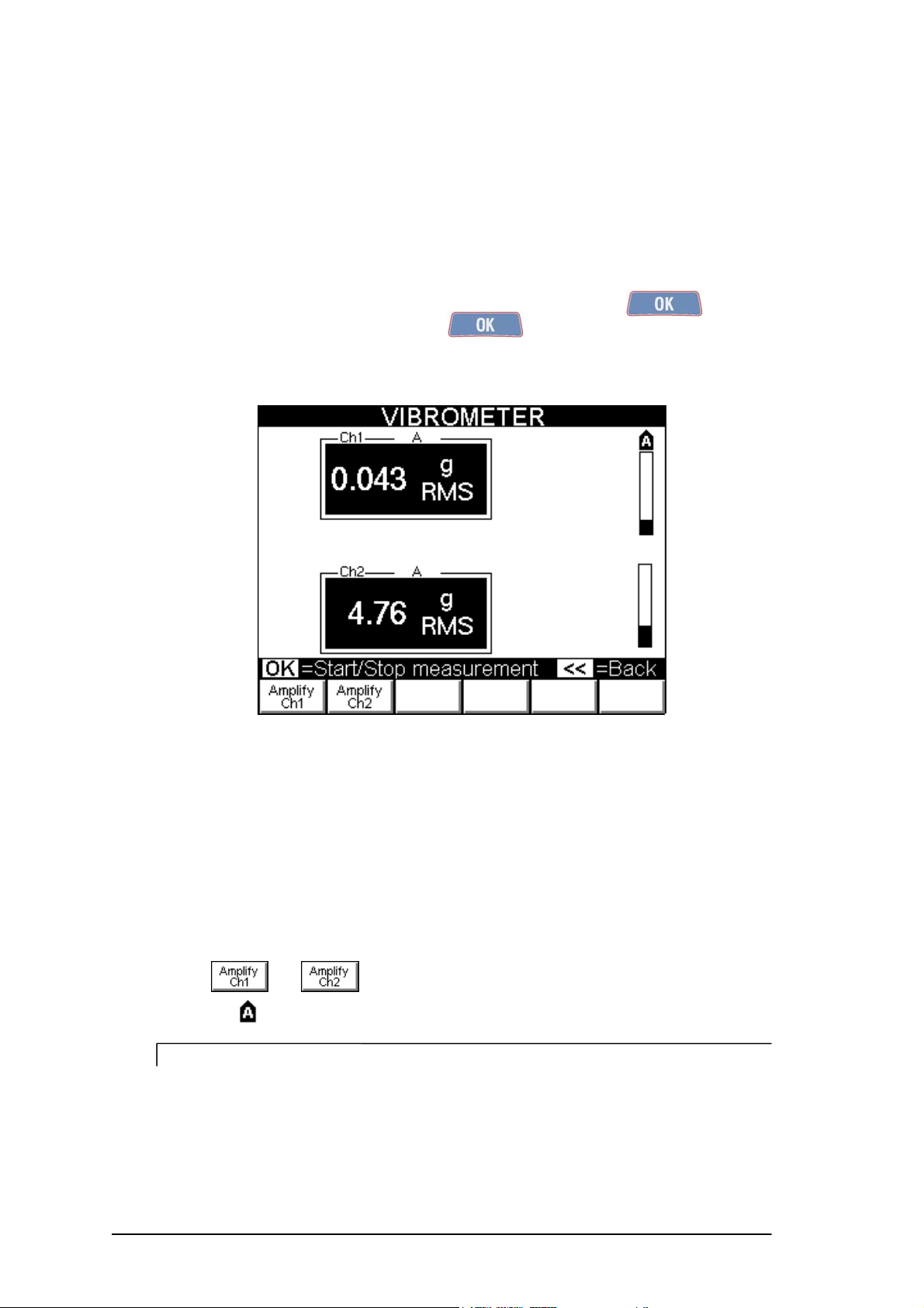
The Measurement page supplies a series of information, organized as shown in the figure:
1
3
8
4
5
1. channel measured
2. measurement information: indicates unit of the sensor (A, V or D) and any
conversion made to supply the overall value (e.g. AÆV means that the measurement
is made with an accelerometer, but the vibration is supplied in speed)
3. overall value of the vibration
4. unit of measurement
5. type of measurement
6. value of the synchronous vibration
7. phase of the synchronous vibration
8. speed rotation of rotor
9. signal level bar
2
6
7
9
10
Vibrometer mode 5 - 3
Page 28
10. amplification status of the channel
N.B.
The values obtained in this mode can be reused to evaluate the operating status of
the instrument by using, for example, the tables and graphs given in Appendix B
of this manual.
The default measurement is that of the total vibration value, but by pressing it is
possible to switch to measurement of the synchronous value: in this mode, information
appears concerning the modulus, phase and speed of rotation. Pressing of allows
return to measurement of the overall. value. N.B. To perform a synchronous measurement,
it is necessary to connect the photocell and make sure that it is positioned correctly (see
Speed monitoring 5-6).
Direct printing of the vibration value (optional).
By connecting the portable printer supplied (optional) then pressing it is possible
to print directly in field the vibration values displayed in the VIBROMETER PAGE
Monitoring in time
The monitoring in time function allows observing (and memorizing if necessary) of the
trend of the overall vibration value plotted against time. For such purpose, it is necessary to
preset a value which is adequate for the parameter by selecting from the following
possibilities:
– 1'' - one second
– 10'' - ten seconds
– 1' - one minute
– 15' – fifteen minutes
After pressing a measurement is made of the overall value, indicated by a
point on the graph; such measurement is automatically repeated according to the preset
time step, and a new point is represented in the graph. Availability of a new measurement is
signalled by momentarily displaying the time step in white on black background
(under the icon with metronome ).
When the number of measurements made exceeds forty, just the most recent forty
measurements are shown in the graph.
Monitoring is stopped by a further pressing of and the typical control
functions of the graphs become available (see 2-5 Functions operating on the graphs).
- Set scale (with which it is also possible display all the measurements made)
- Show cursor
- Change of channel displayed
- List of peaks
5 - 4 Vibrometer mode
Page 29

When and then is selected, the entire monitoring can be saved in a file
for subsequent analysis.
When the acquisition is enabled for both channels, the data save is performed automatically
for both channels in the same file.
N.B.
As access to the Monitoring in time function is gained from the
VIBROMETER screen, the settings used for calculation of the overall value are
the ones selected in the VIBROMETER SETUP screen.
N.B.
The memory allotted for a single monitoring, allows memorizing a maximum of
1024 values per channel: when the limit is reached, the acquisition is stopped
automatically without data loss. For this reason, it is important to use the most
suitable frequency according to the duration of the phenomenon concerned.
Vibrometer mode 5 - 5
Page 30

Monitoring in speed
In many situations it could prove useful to associate the vibration value with that of the
speed of rotation of a shaft; in this way it could be possible to investigate, for example,
how the overall or the synchronous component varies during machine starting or stop
phase, with identification of any critical zones or zones with risk of resonance, which are
best to avoid.
In order to be able to use this function, it is essential to have the tachometric signal;
therefore it is necessary
- to apply a reflecting label on the rotor as reference mark (0°). Starting from this
position, proceed to measure the angles in direction opposite to that of the shaft
rotation.
– connect the photocell and position it correctly (50 – 400 mm), so that the led
located behind it lights up once for each rev. when the reference mark is
illuminated by the light beam. If the operation is not regular, either retract or
approach the photocell, or else incline it with the respect to the workpiece surface.
Speed monitoring can be performed according to two different modes, namely:
- monitoring of overall vibration (overall)
- monitoring of modulus and phase of the vibration synchronous with the speed
of rotation (1xRPM)
An icon on the top part of the page indicates which mode is currently selected; this mode
can be changed by pressing .
Two graphs are always displayed simultaneously in a synchronous monitoring. Such graphs
can be:
– modulus and phase of the vibration of channel 1
– modulus and phase of the vibration of channel 2
– modulus of the vibration for both channels
To switch between the various modes, press
After pressing a vibration measurement is made and a speed reading taken,
these are then plotted by a point on the graph; such measurements are repeated
automatically, with a new point added each time to the graph.
For the sake of convenience, the current rotor speed, expressed in RPM, is displayed at the
top right, alongside the symbol
5 - 6 Vibrometer mode
Page 31

Monitoring is stopped by a further pressing of and the typical graph control
functions become available (see 2-5 Functions operating on the graphs).
- Set scale
- Show cursor
- Change of channel displayed
- List of peaks
When is pressed, the entire monitoring can be saved in a file for subsequent
analysis.
When the acquisition is enabled for both channels, the data save is performed automatically
for both channels in the same file.
N.B.:
The memory allotted for a single monitoring, allows memorizing a maximum of
1024 values per channel: when the limit is reached, the acquisition is stopped
automatically without data loss. For this reason, it is important to use the most
suitable frequency according to the duration of the phenomenon concerned.
Vibrometer mode 5 - 7
Page 32

Page 33

Chapter 6
FFT (Fast Fourier Transform) analyzer mode
A complete analysis of the vibration cannot fail to take into account the study of the
various factors contributing towards forming its overall value. Hence it is essential to be
able to carry out spectrum analysis with FFT (Fast Fourier Transform) algorithm.
Such technique allows splitting and memorizing a measured signal into its component
frequencies in a certain period of time, thus making it easier to discover their causes.
Analysis of the highest peaks in the spectrum, together with analysis of the frequencies to
which they correspond allows determining which are the principle sources of vibration and,
therefore, the aspects on which to act in order to reduce them.
Although a spectrum contains a series of very significant information, its interpretation
requires a certain amount of experience and attention; for this purpose, the material given
in Appendix C – A rapid guide to interpreting a spectrum could be useful.
FFT Setup
The choice of correct settings is vital in order to highlight the significant information in the
spectrum thus separating it from the inevitable background noise.
1. Unit of measurement
Select the unit of measurement in which the vibration is to be supplied; possibilities are as
follows:
– acceleration (g) – enhances the higher frequencies and attenuates the lower ones
– speed (mm/s or inch/s)
– displacement (µm or mils) – enhances the lower frequencies and attenuates the
higher ones.
FFT analyzer mode 6 - 1
Page 34

2. Type of measurement
This is the mode in which each component (line) of the spectrum is applied; it can be:
– RMS (Root Mean Square):
This is the one most typically used, as it is associated with the overall RMS value.
– PK (Peak):
This is the maximum value reached by the component in question in a certain
interval of time;
it is rarely used because it does not provide information about the overall PK value;
line by line it is simply equal to the RMS value multiplied by 1.41.
– PP (Peak-to-Peak):
This is the difference between maximum value and minimum value reached by the
vibration in a certain interval of time;
it is rarely used because it does not provide information about the overall PP value;
line by line it is simply equal to the RMS value multiplied by 2.82.
3. Unit of frequency
It can be chosen from:
- Hz – cycles (revs) per second
– RPM – revs. per minute
N.B.
Obviously the relationship 1 Hz = 60 RPM holds good between the two units
4. Max frequency
This is the maximum frequency of interest in the phenomenon; in practice, it is the
maximum frequency which can be shown in the spectrum. It can be chosen from the
following default values 25, 100, 500, 1000, 2500, 5000, 10000 and 15000 Hz, on the basis
of which the N500 instrument will choose the appropriate frequency for data acquisition.
N.B.
The typical choice, suitable for most situations, is 1000 Hz (60,000 RPM),
coherently with the requirements of ISO 10816-1.
N.B.
One practical consideration normally adopted is that of making sure that the max.
frequency preset is at least 20-30 times that of the frequency of rotation of the shaft
being examined. This allows including in the spectrum also the high frequency zone
where problems relating to the bearings usually occur.
N.B.
With other conditions remaining the same, the choice of a maximum low frequency
(less than 1000 Hz) would cause an appreciable increase in the times required for
acquisition and measurement.
6 - 2 FFT analyzer mode
Page 35

5. N° of lines
Such parameter defines the number of lines used in the FFT algorithm, in practice
associated with the resolution in frequency in the spectrum. This determines how close can
be the frequency of two peaks so that they still remain distinct in the FFT graph. Such
resolution is equal to
f
max
N
linee
therefore to maintain it constant, when the max. frequency is increased, likewise the
number of lines should be increased.
It is useful to remember that the time required for acquisition of the correct number of
samples is exactly equal to the inverse of the resolution; then the time required for data
processing should be added to this time. An example of the relation between resolutionacquisition time may be derived from the following table:
N.B.
The use of an excessively high number of lines is not recommended unless in
situations where an extreme resolution is essential. In fact, such choice would lead
to an increase in calculation times and space required for data saving, often without
adding particular information.
A reasonable choice would be 200, 400 or max. 800 lines, being careful to set a
max. frequency coherent with the situation in question.
6. Average N°
Resolution [Hz] t
5 0.2
2.5 0.4
1.25 0.8
0.625 1.6
0.3125 3.2
acquisition
[sec]
This is the number of spectra which should be calculated and averaged between each other
to increase stability of the measurement. Four averages are more than sufficient for normal
vibration measurements on rotating machines.
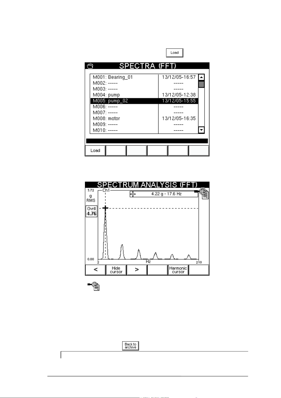
Press to access the SPECTRUM ANALYSIS (FFT) measurement screen.
FFT analyzer mode 6 - 3
Page 36

Spectrum analysis (FFT)
The so-called FFT algorithm is applied to the signals acquired with due respect for the
settings made; in accordance with the recommendations deriving from the mathematical
treatment from which it has been taken, such numeric processing is preceded by
application of a Hanning window to the acquired signal. This allows attenuating the edge
effects due to digitizing as well as reducing phenomena of leakage in the spectrum.
The Measurement page appears like the one shown in the figure. It is organized so as to
maximize as much as possible the area dedicated for representation of the FFT graph.
A box Ovrll is located on the left side giving the overall value of the signal for the channel
displayed; it has the same units of measurement as those of the FFT. Such information
allows monitoring the total vibration, also during the analysis of its single components.
Beside the usual graphic control functions (see 2-5 Functions operating on graphs),
namely:
- Set scale
- Show cursor
- Change of displayed channel
- List of peaks in order to display the list of highest peaks in the spectrum (see 2-8
List of peaks).
the following are available:
– Waveform (see 6-6 Waveform function).
– Trigger Setup to set a trigger to be used for starting the acquisition
(see 6-6 Trigger Setup).
6 - 4 FFT analyzer mode
Page 37

Harmonic cursor
When the cursor is displayed on an FFT graph (see. 2-6 Use of the cursor), it means that
a special mode known as harmonic cursor is available.
The frequency at which the cursor is currently positioned when is pressed, is
considered as the fundamental frequency of the signal under examination, and on the graph
all the harmonics of higher order (2nd, 3rd, 4th, …) are marked
Shifting of the cursor, which varies the frequency considered as fundamental, causes the
automatic updating of the position of all the multiple ones.
Use of the harmonic cursor allows easy recognition in the spectrum of families of peaks in
correspondence of frequencies, which are multiples between each other, and typically
indicative of special defects (see Appendix C).
FFT analyzer mode 6 - 5
Page 38

Waveform function
In the second series of functions (accessed by pressing ) is present
which allows access to a page where the vibration signals are shown in relation to time.
In this mode, the N500 instrument can be used as an actual oscilloscope, and further
enhances the variety of information which can be deduced from the vibration signals.
This mode also contains all the typical graph control functions (see 2-5 Functions
operating on graphs).
It is possible to return to SPECTRUM ANALYSIS by selecting then .
Trigger Setup
In certain cases, it could be useful for acquisition not to start with the pressing of
by the operator, rather with a certain condition associated with the phenomenon being
observed; this is possible by enabling the so-called trigger. In this way, the measurement
does not started immediately after pressing , but only when the signal of the
trigger channel exceeds a preset threshold.
Operation of a trigger can be enabled in two distinct modes, namely:
– Cont. (continuous mode)
– Single (single measurement)
and requires presetting of
– a channel
– a threshold
6 - 6 FFT analyzer mode
Page 39

One of the most frequent uses is the so-called Impact test: A hammer is used to stress a
structure and to cause it to vibrate in order to determine its natural frequencies. For such
purpose, a sensor should be placed in the zone to be examined and a threshold value
chosen, which is higher than the background noise read, but lower than that produced by
the hammering with which the structure is stressed.
N.B.
After enabling the trigger and selecting the required settings, press
to return to the Measurement page in which the mode selected for the trigger is
specified by a specific icon:
– continuous mode
– "single measurement" mode
Now merely press , and wait for the trigger threshold to be exceeded.
If it is required to stop the procedure manually (before or after exceeding the threshold),
just press again.
1. Modes
This is the parameter which indicates whether the trigger is:
– OFF (disabled) :
the measurement is started and stopped manually by the operator on pressing
– Cont. (enabled in continuous mode) :
acquisition is started when the signal exceeds the trigger threshold, and continues
until the operator stops it manually (by pressing )
– Single (enabled in “single measurement” mode) :
When the signal exceeds the trigger threshold, a single measurement is made (duly
observing the parameters set for the FFT), then the acquisition is stopped
automatically; this is the most frequently used mode because it allows analyzing
phenomena of transitory type; by suitably presetting the FFT parameters, it is
possible to obtain an acquisition time sufficiently long for containing all the
important information.
Subsequent acquisitions would only succeed in capturing noise, therefore they
would be counter-productive.
FFT analyzer mode 6 - 7
Page 40

When the trigger is enabled, the following settings become visible in the TRIGGER
SETUP page:
– Channel
– Threshold
2. Channel
This indicates on which channel (Ch1 or Ch2) to make the comparison between the signal
value and the threshold value in order to activate the acquisition.
N.B.
If just one of the two measuring channels is enabled, obviously choice of the trigger
channel is obligatory, hence it is forced automatically.
3. Threshold
This is the level which the signal must exceed (in a leading edge of the waveform) in order
for the acquisition to be started automatically. The selection of a suitable value is normally
one of the most delicate operations, but by using the N500 instrument it is considerably
simplified. The graph at the bottom of the page shows in real time the signal of the trigger
channel (in continuous line) and the current threshold (broken line). Hence the effect of
different values can be assessed immediately, thus making it easier to make a rapid choice
of the value considered most appropriate.
6 - 8 FFT analyzer mode
Page 41
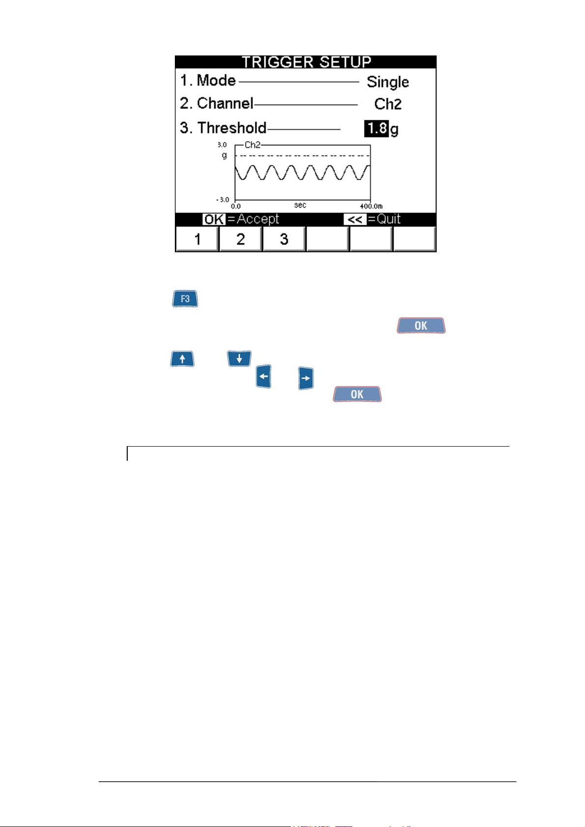
After pressing the threshold value can be preset in two ways, namely:
– By typing, using the numeric keyboard (only after pressing , it is possible
to shift the broken line in the graph);
– by using and to increase or decrease the value of a single digit,
which can be selected with and (the broken line in the graph is shifted
immediately, however at the end, pressing of is always necessary in order
to confirm).
N.B.
The trigger threshold should always be set in the unit of natural measurement of
the sensor. However, in the Measurement page, it is possible to supply the vibration
in other units even if this is not recommended when making measurements with
the trigger enabled.
FFT analyzer mode 6 - 9
Page 42

6 - 10 FFT analyzer mode
Page 43

Chapter 7
Balancer mode
One of the causes of vibration most frequently encountered in actual practice, is the
unbalance of a rotating part (lack of uniformity of the mass about its axis of rotation); such
unbalance can be corrected with a balancing procedure.
The N500 instrument allows balancing any rotor under service conditions in one or two
planes, by using one or two vibration pick-ups and a photocell.
Ad hoc procedures have been drawn up for the most frequent situations (balancing on one
plane with just one sensor and balancing on two planes with two sensors). These
procedures guide the operator step-by-step through the sequence of operations. A general
guided procedure is available for all the other cases (rarely used).
Some rules to be observed in order to perform correct balancing are as follows:
- place the sensors as close as possible to the supports of the rotor to be balanced, by
using the magnetic base or by fastening via a tapped hole to ensure good
repeatability;
- apply a reflecting label on the rotor as reference mark (0°). The angles are measured,
starting from this position, in direction opposite to that of shaft rotation.
– Connect the photocell and place it in correct position (50 – 400 mm), so that the led
at the back of the photocell lights up only just once per rev. when the light beam
illuminates the reference mark. If operation is incorrect, either retract or approach
the photocell or else incline it with respect to the workpiece surface.
For further consideration, see attached brochure Balancing accuracy for rigid rotors.
The balancing procedure consists of two parts, namely:
– calibration: a series of spins allows determining the parameters required for balancing
in the case of a given rotor
– measurement of the unbalance and calculation of the correction.
Balancer mode 7 - 1
Page 44

As the calibration is normally a laborious procedure, the parameters derived should be
memorized, then called in the case of subsequent maintenance work on the same machine.
This is possible via the balancing programs: a program is defined with a series of settings in
order to work on a particular rotor and it contains all the information and data acquired
regarding such rotor. It is possible to save the current program at any moment in a special
archive so that it is available at later dates.
N.B.
If it is required to use data and parameters of a previously stored program, it is
essential to mount the transducer in exactly the same position on the rotor.
Selection of the balancing program
When the balancing function is selected, a page is presented to the operator in which to
select the balancing program to be used, choosing between the following options:
– New program
– Loading of program from archive
– Use of current program (only available if a program has been previously created or
loaded)
7 - 2 Balancer mode
Page 45
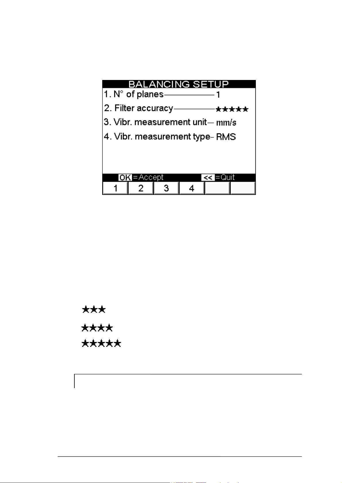
1. New program – BALANCING SETUP
The creation of a new program entails setting of a series of parameters. This is done in the
BALANCING SETUP screen.
1. Number of planes
This is the number of planes on which to act to correct the unbalance of the
rotor. The number can be 1 or 2.
2. Filter accuracy
Balancing under not particularly stable signal conditions is certainly critical and
needs acquisition for longer times in order to obtain a satisfactory quality of the
value measured. This can be achieved by acting on the filter accuracy:
acquisition made with a broad filter: faster, but only suitable for
particularly stable signal conditions (high unbalance values).
acquisition made with a narrow filter: suitable in most conditions.
acquisition made with a very narrow filter: suitable for
particularly critical signal conditions (low unbalance values);
requires longer times
N.B.:
Depending on the accuracy selected for the filter, the instrument automatically
determines the number of revs. necessary for each acquisition. As it could be
necessary to have up to some hundred revs. in certain situations, the time required
for each measurement could likewise be equal to some tens of a second. Taking
into account that a certain number of consecutive acquisitions is necessary so that
the quality of the measurement can reach acceptable levels, the time required for an
acquisition could also entail several minutes in the case of slow rotors.
Balancer mode 7 - 3
Page 46

For example, for a rotor with speed of rotation 600 RPM, it could be necessary to
wait up to 10 seconds before being able to view the first result of the measurement.
3. Unit of measurement of the vibration
This is the unit of measurement in which to supply the vibration to the sensors:
– acceleration (g (acc))
– speed (mm/s, inc/s)
– displacement (µm or mils)
N.B.
In order to avoid possible confusion with grams (often used for expressing the
unbalance in the metric system), in the Balancing functions, the symbol
g (1 g = 9.81 m/s2) is accompanied by the explicit indication acc (acceleration)
given alongside between brackets.
4. Type of vibration measurement
The vibration measured by the sensors can be expressed in three different types:
- RMS (Root Mean Square):
This is the average value of the vibration previously squared;
It is the one typically used, especially for measurements of acceleration or
speed.
- PK (Peak):
This is the maximum value reached by the vibration in a certain interval of
time.
- PP (Peak-to-Peak):
This is the difference between maximum value and minimum value reached
by the vibration in a certain interval of time;
It is normally used for measuring displacement..
Confirmation of the settings made (with ) creates a new balancing program
not associated with any name, seeing as though it is directly accessible as current program.
Only when saving in the archive, will there be a request to the operator to enter a special
name which will characterize it from that moment on.
7 - 4 Balancer mode
Page 47
2. Load program from archive
When this option is selected, access is gained to the program archive.
Arrow keys and allows scrolling the 10 available positions, thus selecting the
required program (visible in negative, i.e. with white writing on black background); the
program can then be loaded by pressing .
If it is not possible to carry out the operation correctly (e.g. attempt made to load a
program from an empty position, indicated by the symbol -----), an error message appears
in the black band in the bottom area of the page.
After loading, the following is displayed:
– the measurement and unbalance correction screen, if the calibration procedure has
already been completed;
– the calibration screen, if not.
3. Use current program
This option allows resuming the last program used (new or loaded), exactly from the point
where it had been abandoned.
Caution
:
When the instrument is switched off, this causes loss of unsaved data (and
therefore of the current program); hence this option is not initially available when
the instrument is switched on again; it becomes available only after a program has
been created or loaded from the archive.
Balancer mode 7 - 5
Page 48

Calibration sequence
The calibration operation, necessary for assessing the unbalance of a rotor, is normally a
procedure consisting of various steps. Above all, for the most common two cases, it
consists of:
- Calibration for balancing on one plane:
1) first spin without test weight
2) second spin with test weight on the balancing plane
- Calibration for balancing on two planes:
1) first spin without test weight
2) second spin with test weight only on the first balancing plane
3) third spin with test weight only on the second balancing plane
For the two configurations
– correction on one plane with one sensor
– correction on two planes with two sensors
The calibration sequence screen on the N500 instrument is organized as in the figures.
1
2
3
5
4
7
6
8
9
10
1
2
3
5
4
6
7
8
9
10
7 - 6 Balancer mode
Page 49

1 - number and name of the balancing program (if loaded from the archive),
or else ----
2 - current speed of rotation, in RPM
3 - layout of the position of the sensors and correction planes on the rotor; indication
of the plane on which to apply the test weight
N.B.
This representation is approximate only; the sensors and correction planes can be
chosen in any position relative to each other (external sensors or sensors inside
planes, ... ) since the calibration serves especially for determining correct
parameters for balancing in any configuration.
4 - value and angular position of any test weight
5 - indication of the vibration component synchronous with the rotation (unbalance) in
value and phase for every measuring channel
6 - average speed of rotation and filter accuracy with which the vibration has been
measured
N.B.
The average speed value is highly important because the calibration procedure can
only be considered as properly performed if between one step and the other, such
speed does not exhibit differences exceeding 5%. It is up to the operator to check
for this condition.
7 - indication of the number of calibration step selected
8 - indication of the status of the calibration steps
completed
to be done
9 - instructions for the current calibration step
10 - functions for selecting the calibration step
: go the previous step
: go to next step (if the current step is the last step of the sequence,
this function, which is indicated by , ends the calibration and
loads the unbalance measuring page).
N.B.
When each already completed step is selected, the available data appear on the
monitor (vibration, average measuring speed, ... ). Such information is useful, also at
a later date, to decide whether to repeat or not to repeat the measurement.
N.B.
Although it is advisable to perform the calibration steps in the order in which they
appear, it is perfectly possible to select a different order according to your
particular requirements.
Balancer mode 7 - 7
Page 50
Execution of measurement
To start the measurement in any of these steps, press ; a pop-up panel appears
showing, in real time, the quality of the current measurement (for each channel).
The higher is the level of the bars, the better will be the quality of the measurement (which
is averaged over time). After reaching the required level, stop the measurement again by
pressing .
If the operator decides to accept the value, then he must press corresponding to
the option , which flashes in order to warn the operator the importance of
pressing it.
When the measurement is accepted, the corresponding calibration step is indicated as
complete .
N.B.
Unstable signals produce measurements whose quality is unable to reach acceptable
levels; under these conditions, it is advisable to increase filter accuracy
(see 7-3 Filter accuracy) and consequently repeat the entire procedure.
N.B.
If the quality of a particular measurement has been altered by a special event (e.g.
an impact), the time required to go back to it could be excessively long; to speed it
up, the measurement can be reset manually by pressing .
7 - 8 Balancer mode
Page 51

Test weight
Calibration requires the use of a test weight, to be applied in succession on the various
correction planes. These two parameters should be preset, with the appropriate
functions and by typing the appropriate values with the numeric
keypad, and confirming with .
To cover the various operational requirements when balancing on two planes, it is
possible to specify a different test weight (value and angular position) on plane 1 and on
plane 2.
N.B.
The value of the test weight should be indicated in general units U. The operator
can decide independently to make these U correspond to the physical units
preferred by him, bearing in mind that also the unbalance and necessary
correction will be indicated in the same units U.
Caution
Correct choice has been made of the test weight if it produces, in each of the spins,
a sufficient variation in the vibration compared to that of the initial spin.
This may be considered satisfactory if we have at least one from the following:
- variation in module of at least 30%
- variation in phase of at least 30°
:
Balancer mode 7 - 9
Page 52
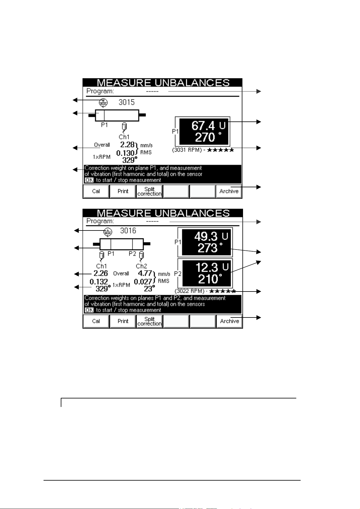
Unbalance measurement and calculation of the correction
In appearance the UNBALANCE MEASUREMENT page is very similar to the calibration
page:
1
2
3
4
6
7
2
3
6
7
5
8
1
4
5
8
and the following information is given:
1 – number and name of the balancing program (when loaded from the archive),
otherwise ----
2 – current speed of rotation, in RPM
3 – layout of the position of the sensors and correction planes on the rotor
N.B.
This representation is approximate only; the sensors and correction planes can be
chosen in any position relative to each other (external sensors or sensors inside the
planes, ... ) since the calibration serves especially for determining correct
parameters for balancing in any configuration..
7 - 10 Balancer mode
Page 53

4 – indication of the correction weight, in value and position on every plane.
N.B.
The module is indicated in general units U, corresponding to those used in setting
the test weight. As the program makes use of correction through addition of
material, the position indicated is the one where to add the correction weight.
When it is required to proceed by removal of material, act in a position
diametrically opposite (add 180° to the displayed phase)
5 – average speed of rotation and filter accuracy with which the unbalance has been
measured
Caution:
The average speed value is important because it allows checking whether the
measurement has been made at a speed not too different from that used in the
calibration spins (differences less than 5%). Owing to small amounts of non
linearity always preset in actual practice, it is not advisable to proceed to calculate
the correction at a speed too widely different from the calibration speed. Checking
of this condition is up to the operator.
6 – value and phase of the vibration synchronous with the rotation (1xRPM) and total
value(Overall) vibration measured via the sensors
N.B.
This information is considerably important as indicator of the reliability of the
balancing: what concerns us in actual practice is to reduce the vibration to under a
certain value considered as tolerable (see Appendix B). However reduction of the
unbalance only has effect on the 1xRPM component. A low value of this
component, accompanied by a high Overall indicates problems differing from those
of unbalance, which, therefore, cannot be corrected by balancing.
7 – instructions for unbalance measurement and calculation of the correction
8 – functions available
: calibration procedure
N.B.
If the calibration procedure has not been completed, this button starts flashing, to
warn the operator to return to the calibration procedure before being able to make
unbalance measurements. If not, indication is already given of the correction
weights and positions where to act, deduced from the calibration spins.
Balancer mode 7 - 11
Page 54

: direct printing of a balancing certificate by using the portable printer
provided (optional). The certificate gives the unbalances on the
correction planes (in units U), as well as the values of vibration (overall
and synchronous) of these planes. The following is an example of this
certificate:
: function involving splitting of the correction weight on two presettable
angles (see 7-13 Splitting of correction weight. )
: : shows the program archive (to allow saving or eliminating a program)
As in calibration, to start or stop measurement, press ; while the
measurement is active a pop-up appears to indicate the quality of measurement of each
channel.
After making the corrections indicated, the measurement-correction procedure can be
repeated until the required conditions are met (typically vibration measured by the
sensors lower than a certain value).
7 - 12 Balancer mode
Page 55

Splitting of correction weight
In this page it is possible to select between the correction modes:
- by addition of material
- by removal of material
By pressing push buttons and respectively.
In certain practical situations it is not possible to correct in the position calculated
theoretically as optimum position: in the case of a fan, for example, such position could fall
in the gap between two blades, where obviously it is not possible to add or remove
material. However, it is often the case also for uniform rotors, to prefer to correct where
holes are already present, or else to avoid acting in particular zones.
The split function of the N500 function calculates the weights to be applied or to remove
corresponding to any two positions α1 and α2, so that their effects are equivalent to those
of the correction calculated by the balancing algorithm.
When or is pressed, the user can assign the most appropriate value to
these two positions, by selecting from those effectively available in practice for that
particular rotor. By pressing the two corresponding correction weights are
automatically calculated and displayed.
Such operation can be performed separately on each of the planes, after selecting the
required one by pressing .
Balancer mode 7 - 13
Page 56

Caution:
Whatever the value of α1 and α2, the angle of
revolution is subdivided into two parts, one part
convex (<180°) and the other concave (>180°).
In order to carry out the splitting, angles α1 and α2
should be chosen so that the correction position
calculated during balancing, lies within the convex
zone.
If not, such splitting would be impossible, and the
N500 instrument would indicate zero as correction
weight for both positions α1 and α2.
N.B.:
It is useful to observe that the more the α1 and α2 positions are further apart from
the position calculated in balancing, the higher must be the values of the
corresponding weights. Hence it is advisable to select α1 and α2 as close as possible
to the correction angle obtained by the balancing operation, or at least to make sure
that they differ by less than 150°.
Saving of a balancing program
After displaying the program archive, proceed to select (with and the
position in which to save the current program.
When is pressed, a pop-up appears in which to enter the program name, as
explained in 2-3 Alphanumeric keypad..
Instead, when is pressed, the selected program can be eliminated, provided it is
not the current one .
Instead with it is possible to eliminate all the balancing programs contained in the
archive.
7 - 14 Balancer mode
Page 57

Chapter 8
Data manager mode
The N500 instrument allows saving the measurements made (FFT, waveforms and
monitoring) in special archives, which can be managed through this special function
directly accessible from the home screen.
Upon pressing a MEASUREMENT ARCHIVE screen appears where it is
possible to select between the following possibilities:
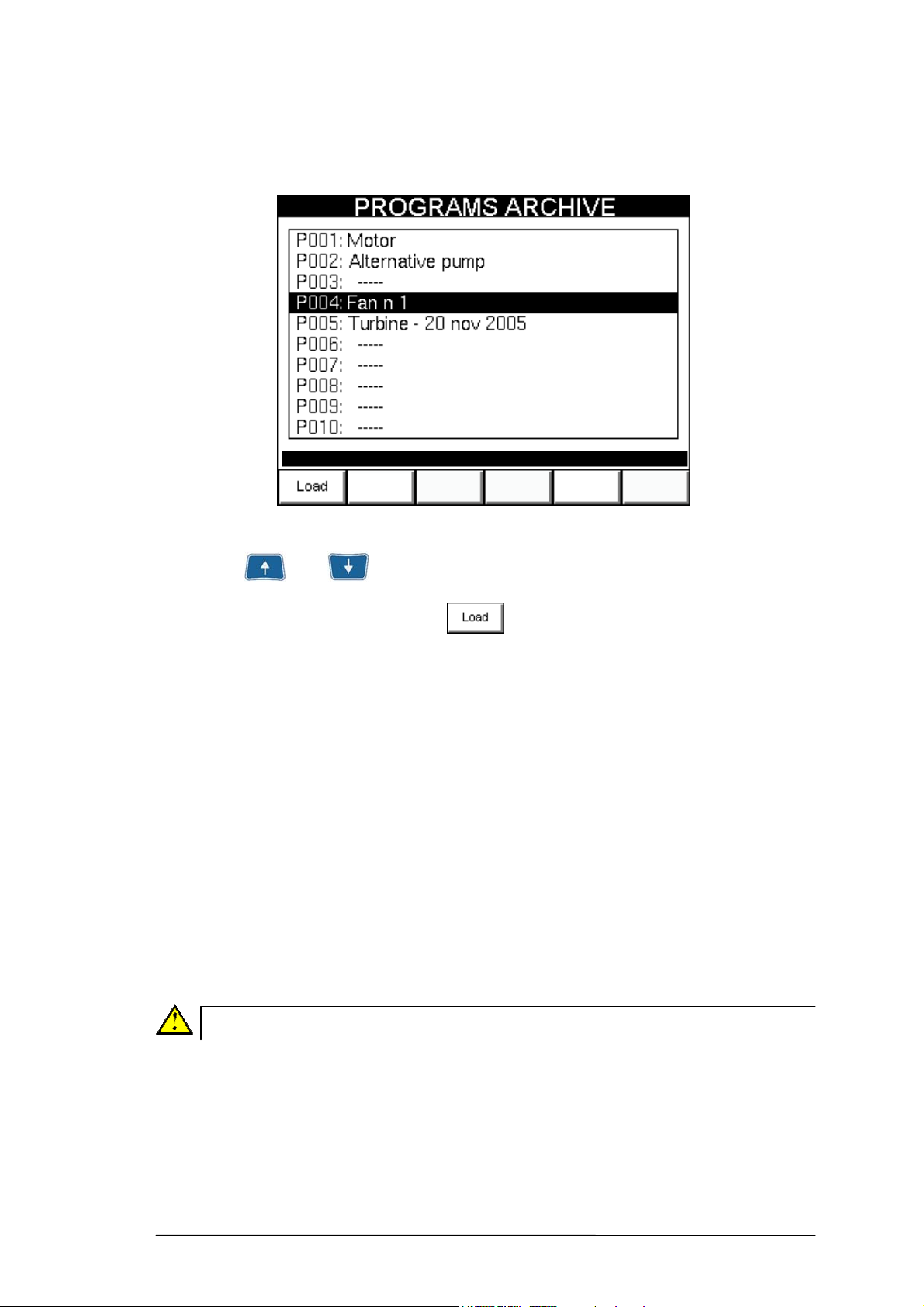
– Data management (i.e. rename or eliminate the data present);
– Copy the data on the USB key (pen drive) supplied, leaving a copy of the data on the
N500 instrument;
– Shift the data on the USB key (pen drive) supplied, thus deleting the data from the
N500 instrument;
– send archive to PC using CEMB PoInTer software
– load (display) measurements already in the archive.
Archive management
Measurements saved with the N500 instrument are subdivided by type into different
archives:
– waveforms
– FFT
– Monitoring in time
– Monitoring in speed
A fifth archive is reserved for the images in the screens,captured by pressing .
(see 2-10 - Capture and saving of displayed images).
Data manager mode 8 - 1
Page 58

When one of the archives in selected in the SELECT DATA MANAGER screen, its
contents will be displayed making distinction between empty positions (-----), and occupied
positions (name, date and time of save).
After selecting one of the items of data, the latter can be renamed or eliminated (to free
space) if it no longer serves.
To fully clear the archive, press then confirm by pressing .
N.B.
The archive can be scrolled by one position at a time with the and
keys, or more quickly with and (+10 and –10 respectively).
Copying /shifting archive on USB key
The data on the N500 instrument can be copied or shifted to the USB key supplied, and
then easily imported on to an ordinary PC with CEMB PoInTer software (see Chap. 9).
However without such software it is possible to use the images captured in the various
screens, e.g. by attaching them to any documentation produced with one of the various text
editors.
Caution
The pendrive supplied by CEMB is formatted for use on either the N500
instrument or on a standard PC with Windows or Linux operating system. Never,
under any circumstances whatsoever, proceed to a new formatting of the pendrive
otherwise it could no longer be used with the N500 instrument. In such case,
contact the CEMB Technical Service.
8 - 2 Data manager mode
Page 59

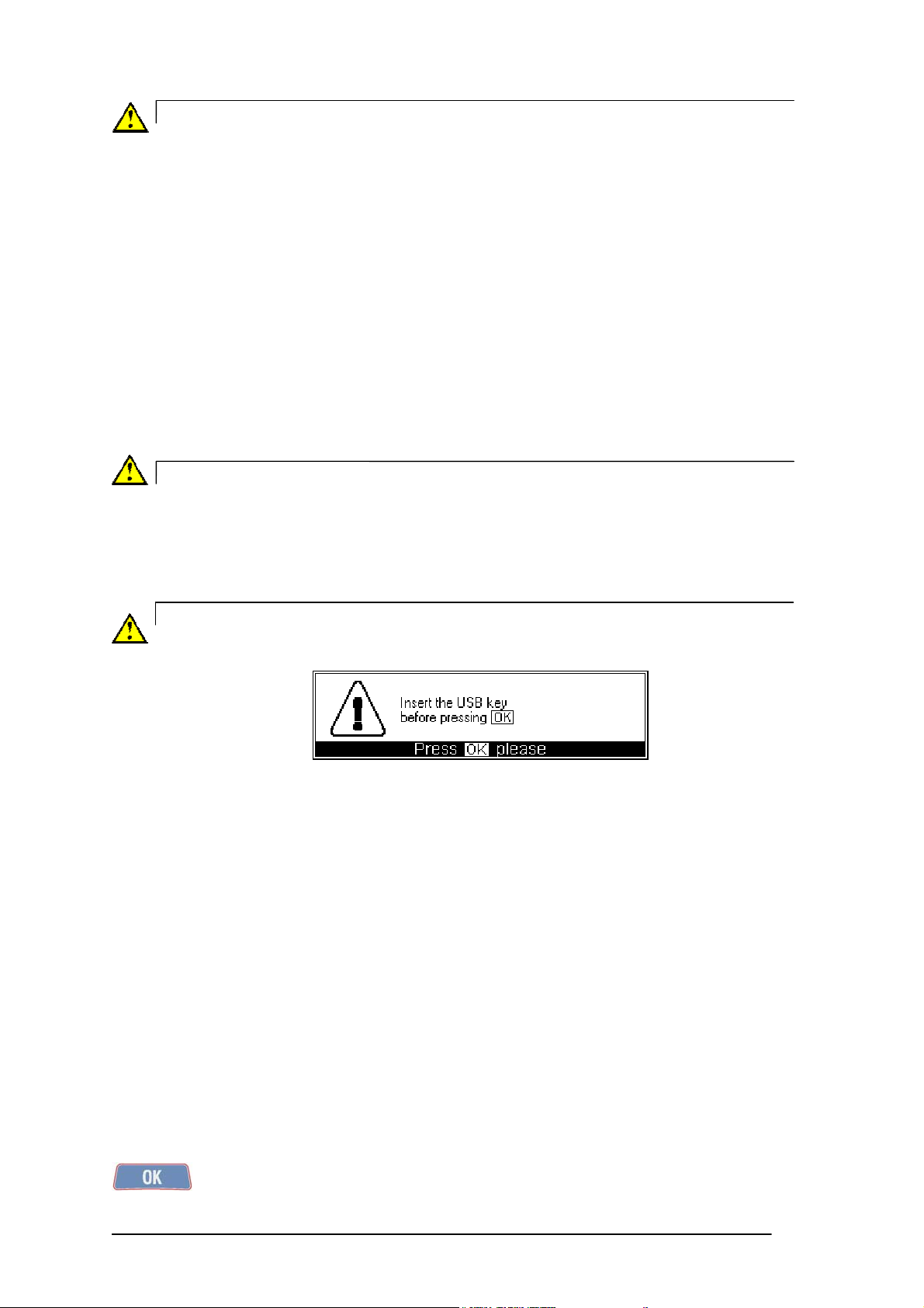
After inserting the pen drive in one of the two USB ports on the instrument
it is necessary to select which archive/archives to be transferred. These will be marked with
the symbol placed alongside its/their name.
Pressing of
causes starting of the data transfer process, indicated by the
pop-up wait message
At the end, the symbol indicates that the operation has been concluded successfully.
Instead, any errors are given in the same pop-up message alongside the symbol .
Data manager mode 8 - 3
Page 60
Caution
Never extract the USB key while the pop-up wait message is showed and before
proceeding, wait at least for its led to flash slowly. If flashing is rapid, it means that
the data transfer is still in progress and extracting the pen drive could block the
system, besides causing data loss. In such case, it could be necessary to reboot the
instrument.
The archives are copied on the pen drive inside the Db_N500 folder, in a specially created
subdirectory, whose name is the data of transfer in YYMMDD format (e.g. 051221 for 21
December 2005). In order to allow downloading of two or more archives in the same day,
there is provision for an adding a suffix “_* ” to this name where * is a letter assigned
progressively from A to Z.
Obviously it is not possible to transfer more the 26 archives on the key on the same day
before proceeding to load them on the PC, with the CEMB PoInTer software
(see 9-7 – Loading of new measurements in the archive), or manually.
Caution:
Never shift, rename or delete the folders or files downloaded on the pen drive from
the N500 instrument because this could cause malfunctions or incompatibility of
the CEMB PoInTer software.
Caution:
If the following error message appears
st
even with the pen drive inserted correctly, there could be a problem of recognition of
the key.
Try removing it, then inserting it again, switching the instrument off and on again if
necessary. If the problem persists, contact the Technical Service Department.
Sending archive to PC (CEMB PoInTer software required)
Data stored in the N500 instrument can be sent directly to a PC equipped with CEMB
PoInTer software, version 2.6 or greater.
To complete this operation successfully, connect the N500 instrument to the serial port
(RS232) of the PC using the cable supplied by CEMB for this purpose. After starting the
'Import data' function in the CEMB PoInTer software, wait until the communication in
progress message appears (see 9-6 - Reading measurements saved on the N500
instrument
key.
.), then select the archives to be sent on the N500 instrument and finally press
; the procedure is similar to that followed for the transfer of data using a USB
8 - 4 Data manager mode
Page 61
Display of measurements present in the archive
It is possible to display all the measurements and images saved in the N500 instrument by
selecting them from the relative archive and pressing
This makes it very easy to obtain comparisons and to make assessments directly "in field ".
The various data are presented in screens wholly similar to the corresponding measurement
screens.
in which the icon at the top right serves for reminding the user that being display
pages, it is not possible, for example, to start a new acquisition.
Instead, the following functions are available
- set scale
- show cursor
- change of channel displayed (only for two-channel measurement)
- list of peaks (only for FFT)
To quit the display screens, press
N.B.:
available.
Data manager mode 8 - 5
Obviously if an item from the image archive is loaded, no function is
Page 62

8 - 6 Data manager mode
Page 63

Chapter 9
CEMB PoInTer Program (optional)
The data collected and memorized with the N500 instrument can readily imported to a PC
(directly or using a USB key), and subsequently analyzed, processed, compared, printed.
Such operation is considerably facilitated by using the CEMB PoInTer (Portable
Instruments Terminal) software, available for Windows operating systems.
Its main page
1 2 3
can be imagined as being subdivided into three zones, which allow the following items to
be controlled respectively:
1 – archive of measuring points
2 – measurements available for the point selected
3 – list of measurements to be plotted in a graph
System requirements
Installation and use of the CEMB PoInTer program require:
- processor: at least Intel Pentium IV 1GHz or equivalent Athlon;
- memory: 512MB (recommended: 1GB or higher);
- disk space: at least 300MB free before installation (this does not include the space
occupied subsequently by the data archive);
- Operating system:
- Microsoft Windows 2000 at least Service Pack 4
- Microsoft Windows XP at least Service Pack 2
- Microsoft Windows Vista
- Display resolution 1024x768 or higher
CEMB PoInTer program 9 - 1
Page 64

Installation and registration
For installation of the CEMB PoInTer software, proceed to run the setup.exe program,
contained in the CD-ROM, and then click on the button without changing any
option.
In this way the software will be installed in the default program directory.
When running the software for the first time, it is necessary to select the default language
from those proposed; when the button is pressed, a pop-up appears with the
serial number (S/N) of the software and a request appears to enter the corresponding
activation code.
This code can be obtained by
contacting via E-mail the
CEMB Technical Service,
Instrument Division
(see www.cemb.com)
by specifying the object:
"CEMB PoInTer activation code"
and by citing in the message
your own data and serial number (S/N)
visible in the pop-up.
The CEMB Technical Service will reply
with an e-mail containing the
corresponding activation code (AC)
The activation code should be entered
to complete the registration procedure
and to allow the software to be used.
N.B.
Pressing allows temporary use of the software whilst waiting to
receive the correct activation code from CEMB assistance.
9 - 2 CEMB PoInTer Program
Page 65

N.B.
To ensure correct installation and activation of the product, it is advisable to have
the Administrator rights on the PC used; this is possible by making a login as
Administrator user.
Caution:
Installation of the CEMB PoInTer software requires a different activation code on
each PC, each one of which must be requested from CEMB by the abovementioned procedures.
Archive for measurement points
A measurement archive, especially if of large size,
should be structured in some way for fast and
efficient data access. The CEMB PoInTer software
links each measurement with the point in which it
has been acquired and organizes the various points
in a hierarchical tree structure on four levels.
Suggested interpretation of the tree is:
Area (customer):
This can indicate an actual plant (or else
the name of a customer at whose premises
the measurements have been made);
Station:
This can indicate a department, for
example;
Machine:
This can be a turbine, motor, pump, fan,
…;
Point:
Indicates where the measurements have
been gathered on the machine (e.g. a
certain bearing, one of the supports, …).
Each element of the tree (node) can have one or
more children: in this way several different
configurations can be represented and handled.
CEMB PoInTer program 9 - 3
Page 66
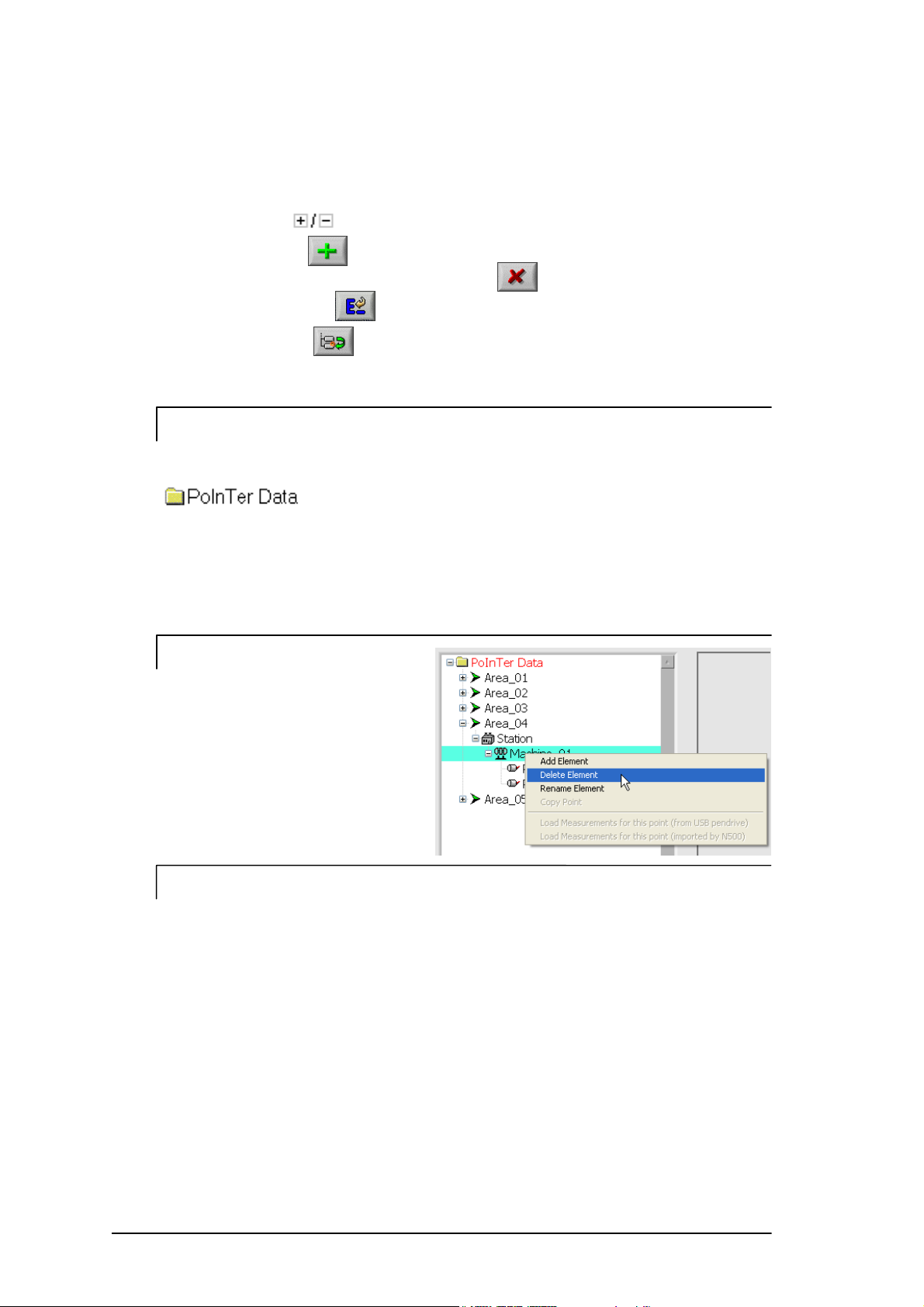
Data Manager
The archive can be fully handled with just a few simple operations using the mouse:
- Select an item : click on the name;
- expand / close a node (i.e. display or hide its children) : double click on the name or
click on the symbol ;
- add an item : click on and type its name;
- eliminate an item (with all its children) : click on , then confirm when asked;
- rename an item : click on and type its new name;
- copy a point : click on ;
N.B.
While the “delete” and “rename” functions act on the item selected, “add item” creates
a child of it. Therefore to insert a new plant, proceed to select the following folder
to create a station, select the plant of which it should form
part, and so on ….
To speed up the operation, together with a plant, also a station, a machine and a
point are automatically created and the user can subsequently rename them
according to his requirements.
N.B.
The functions regarding adding /
eliminating / renaming a node and
the function for copying (just one
point) are accessible from
the contextual menu (select an
item and click with the right mouse
button).
N.B.
While it is sufficient, when creating a plant, station or machine, just to type its
name, for a point it is necessary to also select the settings used (or to be used) for
the FFT measurements (see 6.1 Setup FFT):
- max. frequency (25, 100, 500, 1000, 2500. 5000, 10,000, 15,000 Hz)
- number of lines (100, 200, 400, 800, 1600, 3200)
- unit of measurement (g, mm/s, µm, inc/s, mils)
- type of measurement (RMS, PK, PP)
- number of averages (1, 4, 8, 16)
This ensures that measurements made at a future date on the same point will always
be coherent between each others and therefore comparable.
9 - 4 CEMB PoInTer Program
Page 67

Caution:
The measurement settings are essential data for a point. For this reason they must
be modified after the creation of the point. In the case of incorrect entry, the point
should be eliminated and then recreated.
N.B.
Copying of a point has the effect of creating another one (on the same machine)
with identical measurement settings; therefore such facility is considered as a
practical means for faster creation of similar measuring points, thus avoiding reentering these same parameters for each of them. Then the user only has to rename
them appropriately.
Data protection - Password
A reliable management of an archive requires suitable protection against accidental data
loss. Such protection, in the CEMB PoInTer software, is obtained through the use of a
password. If it is easy to understand how accidental deleting of an item in the archive could
cause an irreparable loss of information, it should also be noted that even just the addition
or renaming of a node could alter the correspondence between the structure of the archive
and the actual situation, thus making data interpretation difficult.
For these reasons, a password allows total inhibition of modification of the archive.
In the default condition (signalled by a closed padlock ) the “eliminate”, “add”, “rename”
and “copy point” functions are disabled. Only by pressing key and entering the correct
password can the padlock be opened and the archive structure modified.
N.B.
The default password is CEMB, but the user can change it
by selecting Change password in the Setup menu.
List of measurements
The measurements available in the archive for the point selected are displayed in a special
window, subdivided into four groups:
- FFT :
- Waveform :
- Monitoring in time :
- Monitoring in speed :
Each measurement can be indicated together with the date and time at the time in which it
was made. Each one of these measurements can be either single channel (only ch1 or only
ch2) or double channel, according to the channels enabled on the N500 instrument when
making the measurement.
N.B.
The measurement settings associated with the point are shown under the FFT list.
CEMB PoInTer program 9 - 5
Page 68

Reading measurements saved on the N500 instrument
CEMB PoInTer software allows you to import measurements saved in the N500
instrument directly to the PC using the connection cable provided for this purpose.
To perform this operation, connect the instrument to the PC’s serial port, then press to
start communication.
Messages and information related to the communication status will be displayed in a
dedicated pop-up window.
The N500 - PC connection takes a few seconds to become successfully established, after
which the user will be informed that they can start transferring data.
This may be done from the N500 instrument as described in 8.4 – Sending archive to PC;
a specific message will be displayed on both the N500 instrument and the PC to confirm
that the operation has been concluded.
The data is saved on the PC in a temporary directory, where it is held until loaded into the
CEMB PoInTer program archives (see following paragraph).
Caution:
The contents of this temporary directory will be deleted when the program is
closed or a new reading is taken from the N500 instrument. We therefore
recommend that data should always be loaded into the PoInTer software archives
as soon as it has been imported from the N500 instrument.
Caution:
If the PC has more than one RS232 port, or a USB/RS232 converter is used, the
number of the COM port used for the connection must be set correctly before
starting data transfer: this information can be obtained from the Device Manager
window in the Windows control panel.
At this point, all that remains is to select it from those listed in the Setup menu Æ
COM N500 Port. If a USB/RS232 converter is used, it must be connected to the
PC before the CEMB PoInTer program is launched.
Note
The user can interrupt data transfer at any time by pressing then closing
communication with the instrument by pressing .
In which case, the N500 instrument will advise that the operation could not be
successfully completed.
9 - 6 CEMB PoInTer Program
Page 69

Loading of new measurements in the archive
New measurements can be loaded into the archive from a USB key (see 8.2 -
Copying/shifting archive on USB key), or from those imported directly from the N500
instrument and saved in a temporary directory (see previous paragraph). After selecting the
point at which they are to be loaded, press or to open a panel in which
files with the following extensions can be selected:
- fft
- wfm (waveform)
- mnT (monitoring in time)
- mnV (monitoring in speed of the total value or of the synchronous harmonic 1x)
-
When loading from a USB key, data will be located in specific subdirectories of the
directory entitled Db_N500 (see 8 - 2 Downloading archive to USB key).
Caution:
In every point of the archive it is possible to load measurements with settings that
differ from those specified for the same point: these measurements are highlighted
with the symbol . In this case, the user must take particular care when
displaying inhomogeneous measurements in the same graph.
Caution:
The types of monitoring in speed of just the synchronous component are identified
by the symbol . Hence we can have the following situations:
- no symbol: monitoring in speed of the overall with settings that are
coherent with those preset for the point
- monitoring in speed of the overall with settings differing from
those preset for the point
- monitoring in speed of synchronous component with
settings that are coherent with those preset for the point
- monitoring in speed of the synchronous component with
settings differing from those preset for the point
It is up to the user to pay special attention when deciding to display, in the same
graph, measurements which are not homogeneous with each other.
N.B.
If the structure of a plant is saved on the USB key, and then deleted on the N500
instrument, the corresponding point will be associated directly with each
measurement made subsequently. Hence loading of all the measurements in the
archive can be performed in automatic mode (and not point-by-point) merely by
pressing .
Caution:
Insert the USB key in one of the PC ports before proceeding to load the
measurements.
CEMB PoInTer program 9 - 7
Page 70
Selection and elimination of measurements
A measurement can be eliminated by selecting it with a click and by pressing the
key located under the list of measurements; this causes opening of a pop-up which
requests explicit confirmation before proceeding to the deleting operation. Such operation,
which causes data loss, is only allowed with the padlock open (see 9-5 Data Protection -
Password).
If more than one measurement is to be deleted, this can be done simultaneously after
selecting them
- by holding down the key on the keyboard and clicking on them one-by-one
- by holding down the key on the keyboard and clicking on the first and last
measurement of the block to be taken as a whole
- by pressing to make a selection between two dates, each one of which can
be either typed , or chosen on a calendar that can be viewed by
pressing .
List of measurements to be plotted in a graph
To select the measurements to be shown in a graph, proceed to select them from those
available and add them to the special list by pressing , or else by double clicking on
them. Instead, to remove them from this list, either press , or double click on
them.
N.B.
To add a measurement to the list, it does not necessarily have to be of the same
type as the ones already present and may originate from any point. The software
automatically makes any conversions necessary, but this can create confusion for
data interpretation if due attention is not paid.
Caution:
Inhomogeneous measurements (e.g. acceleration and speed, or acceleration and
movement) cannot be displayed in the same graph: in this case, the only solution is
to display them in separate graphs.
In the case of FFT or waveform (but only if all of the same point), two different display
modes are available:
- : each measurement is represented just as it is, together with all the other ones
(advisable only if the number of measurement is small, typically lower than 5);
- : an overall vibration is calculated for each measurement and is then represented ;
the one obtained is a graph of the trend of the overall value in subsequent
measurements. This has the advantage of retaining clarity also in the case of a large
number of measurements.
To access the graph display page, press the following key .
9 - 8 CEMB PoInTer Program
Page 71

Display of graphs
2
1
4
3
5
1 – area of the graph
2 – list of measurements plotted (indicating the channel to which they belong)
3 – information regarding the cursor
- measurement with which it is associated
- point of the archive to which such measurement belongs
- current co-ordinates
- keys or buttons to shift it
4 – graphic functions:
- dragging of cursor
- zoom
- shifting of graphs in the window
5 – general functions
- return to main screen “Data Manager”
- separate / combine graphs
- add notes
- create certificate (report)
5
N.B.
Return to the "Data Manager" page is possible, besides by pressing
Also by selecting File Æ Return Back from the menu.
Using the Setup Æ measurement unit option it is possible to select between metric
units (g, mm/s, µm) and imperial units (g, inc/s, mils), or Hz and RPM.
CEMB PoInTer program 9 - 9
Page 72

Cursor
A cursor is present on the graph. This cursor is associated, by default, with the first
measurement plotted. This can be changed by clicking on the graph with the right mouse
button and making the required selection in the contextual menu.
The cursor can be shifted by one step at a time either to the left or right with
or else by pressing the arrow keys on the keyboard.
Instead, by selecting , it is possible to click directly on the cursor, then by holding
down the left mouse button, the cursor can be rapidly shifted to the required position
(always on the measurement with which the cursor is associated).
Zoom
By clicking on key it is possible to choose from different zoom modes:
- (enlarge rectangle) : by clicking on a point and dragging the cursor, it is possible
to select the rectangle to be enlarged;
- (zoom x) : by clicking on a point and dragging the cursor, it is possible to select
the portion of the X axis to be enlarged;
- (zoom y) : by clicking on a point and dragging the cursor, it is possible to select
the portion of the Y axis to be enlarged;
- (autoscale) : by clicking on the graph the extremes of the axes are automatically
set to the most appropriate values, based on the information displayed;
- (zoom in) : by clicking on a point the zone around that point is enlarged;
- (zoom out) : by clicking on a point a larger region around that point is displayed;
9 - 10 CEMB PoInTer Program
Page 73

Shifting the graphs in the window
After selecting it is possible to click on a point of the graph, then by holding
down the mouse button, the entire graph can be shifted within the window. In practice,
this corresponds to changing the minimum and maximum limits of both axes, without this,
however, altering the scale. When the cursor is moved outside the window, the graph
returns to the position prior to the shifting.
N.B.
The minimum and maximum values of the axes can be modified one-by-one, by
merely clicking on them and entering a new value via the keyboard.
N.B.
After modifying the zoom, or shifting the graph, it is possible to return to the initial
view with the option of the contextual menu.
Separate/combine graphs
If it is wished to represent two or more measurements, this can be done in a single graph
(default) or in two or more separate graphs (a maximum of three), with one measurement
in each of them. To switch from one mode to the other press or respectively.
CEMB PoInTer program 9 - 11
Page 74

Creation and printing of certificates and reports
Use of the CEMB PoInTer software allows easy creation and printing of vibration analysis
certificates and reports, including data and/or graphs of the measurements taken and
saved using the N500 instrument.
When the key is pressed, the user must select the model (template) required for the
certificate to be produced. This model is a simple HTML file that the same user can create
as required using any type of HTML editor or a word processing program (e.g. Microsoft
Word, OpenOffice Writer, …); however, in both cases it is necessary to save the model in
HTML format once it has been prepared. The CEMB PoInTer program generates the
report automatically replacing some of the default codes in the template with the
corresponding values.
The result is displayed in the Report window, from where it is possible to:
: save the report created, specifying its name and position
: open and display any report previously saved
: print the report displayed, selecting one of the printers installed in the PC
N.B.
If a virtual PDF printer is selected (e.g. PDFCreator, . . .), a PDF format certificate
can be obtained instead of a hard copy.
: exit the Report window
N.B.
To assist the user, the CEMB PoInTer program provides demonstration templates
that can be used as a base for creating others. These models are located in the
certif_templates subfile of the directory in which the program is installed.
N.B.
A list of codes that can be used in the templates and their meanings is shown in
Appendix D.
Caution:
If it is wished to customize one of the templates already present in the certif_templates
folder, it is advisable to save the modified template under a different name. In fact,
a subsequent updating of the
supplied by CEMB.
It is very simple to add notes, comments and analyses to the reports produced with the
CEMB PoInTer program. This can de done by pressing the key, entering the text
and confirming it with the key. This operation must be carried out before generating
the certificate with the key.
PoInTer software would cause overwriting of the
templates
Caution:
Once inserted, the notes and comments will be used for all reports created
thereafter (until the CEMB PoInTer program is closed), unless they are cancelled
by pressing the key.
9 - 12 CEMB PoInTer Program
Page 75

Appendix A
Specification
- Instrument
- Dimensions: approx. 230 x 230 x 58 mm
- Weight: 1.75 kg
- Operating range
- Temperature: from -10° to +50° C
- Humidity in air: from 0 to 95% without condensation
- Power supply
- Rechargeable lithium battery, 6 Ah
- Charging time: less than 5 hours (from fully discharged battery)
- Power supply unit-battery charger for 100-240 V, 50/60 Hz (24 V, 1.5 A)
- Autonomy: over 8 hours with normal use of the instrument
- Display
– ¼ colour VGA TFT 320x240 – 5.7” back-lit
- Keyboard
- 28 keys, including 6 function keys
- Input channels
- 2 measuring channels (DC power supply max 5 mA, enabled or not enabled
automatically according to type of sensor)
- 1 photocell channel (speed and angular reference)
- Sensors which can be connected
- accelerometer
- velocity sensor
- proximity sensor
- general type, with max. signal 5 V-PP
- photocell 60-18.000 RPM
- high speed photocell
– Portable printer (optional)
– Dimensions: 146 x 88 x 65 mm
– Weight: 0.360 kg (without roll of paper)
– Printing on standard or adhesive paper
- Width of paper: 57.5 mm ± 1 mm
Specification A - 1
Page 76

- Measurement specifications
- A/D converter: resolution 24 bit
- Dynamic range: > 100 dB
- Number of averages: from 1 to 16
- Resolution: 100, 200, 400, 800, 1600, 3200 lines
- Frequency range: DC – 15kHz max
- Background noise: typically less than 1.50 µV for a spectrum with 400 lines having
a max. frequency of 1 kHz
- Window: Hanning (always enabled)
- Speed of analysis: 2.5 averages/sec (400 lines – 1kHz)
- Data memorization capacity: max 500 spectra and 150 waveforms or monitoring
- Instrument error limit: 5%
A - 2 Specification
Page 77

Appendix B
Evaluation criteria
TABLE A
MACHINE CATEGORIES BY EVALUATION CRITERIA
Group
according to
ISO 10816
VDI 2056
I – K
II – M Medium sized machines with electric motors from15 to 100 KW, without any special
Machine parts that are closely related to the machine as a whole during normal working
conditions. Grinding and boring machines. Electric motors (up to 15 KW) that need
good balancing, e.g. dentist’s drills, aerosols, high quality electromedical and domestic
appliances.
Jet engine turbines and compressors.
Fast compressors.
foundations. Lathes. Milling machines. Machines and drives up to 300 KW with rigid
construction, without any parts with alternating movement, resting on their own
foundations. Mass produced electric motors with axis height less than 130 mm.
MACHINES
III – G The most common medium category for first approximation. This category includes
machines not found in other categories. Large machines with rigid, heavy foundations,
without any masses with alternating movement. Gas or steam turbines, turbo blowers,
large alternators. Normal motors in general and especially motors whose axis height is
from 130 to 230 mm. Rigid (class A) fans. Parts of machine tools.
IV – T
V – D
VI – S Machines with masses featuring unbalanceable reciprocating movement, mounted on
Large machines with low-rigidity foundations, without any masses with alternating
movement. Turbines, alternators, large motors, on light foundations or on board ship.
Electric motors with axis heights from 230 to 330 mm. Hydraulic machines, centrifugal
pumps. Normal fans on flexible structures (class B).
Turbine gears. High performance machinery: for printing, spinning or papermaking.
Machines with unbalanceable alternating masses, on foundations that are rigid in the
direction of the greatest vibrations.
Fans on vibrating-damping mounts (class C).
Motors with crankshafts with six or more cylinders on their own foundations. Piston
motors for automobiles, goods vehicles, transportation vehicles not set on insulators
during tests. Machinery with unbalanceable masses, such as weaving looms, skimmers,
centrifugal purification plants, washing machines if fitted to rigid baseplates without any
shock absorbers.
flexible foundations.
Machines with free rotating masses, having variable, non-compensable unbalances, with
flexible mounting, operating without rigid connections to other parts, such as: washing
machines, spin-dryer baskets, vibrating sieves, machines for fatigue testing of materials,
vibrating machines for technological processes, beaters for grinders, vibratory equipment.
Agricultural machines, mills, threshing machines.
Engines with 4 or more cylinders mounted on motor vehicles and locomotives.
Diesel engines with 4 or more cylinders.
Marine diesel engines.
Large two-stroke engines.
Evaluation criteria B - 1
Page 78

EVALUATION CRITERIA BASED ON THE SPEED OF
VIBRATION MEASURED ON FIXED PARTS
For almost all machines, the measurement of the total speed of vibration as RMS value on
fixed parts of the structure is able to characterize the machine from the vibratory point-ofview.
The total value is calculated in the frequency range 10 to1000 Hz or else, for slow machines
(< 600 RPM) in the range 2 to 1000 Hz. Reference is made to the max. speed on the
support in the three directions of measurement.
The class to which the machine under test belongs is identified with the aid of Table A.
The graph of page B-3 provides a direct evaluation of the vibratory state, e.g. if the
vibration measurement on the support of a grinding machine (class 1) is 5 mm/s (RMS)
evaluation is: the vibration is not admissible, hence its cause should be investigated and
removed.
The criterion based on the speed is valid for frequencies lying between 10 Hz and 400 Hz.
Under the frequency of 10 Hz it is possible to have incorrect evaluation because the
vibrations, although having permissible speeds, would have prohibitive amplitudes of
displacement.
With frequencies below 10 Hz, it is necessary to consider the criterion based on the
displacements; while for frequencies exceeding 400 Hz, sometimes also in the range from
300 to 400 Hz, evaluation ratings based on speed should be considered with precaution,
because at such frequencies certain phenomena assume a different aspect and it is
necessary to take into account the energy radiated in the surrounding environment as well
as the vibrations of the building or the environment (ships, aircraft, vehicles) and of the
human physiological interferences. For high frequencies, measurements of acceleration
could prove useful.
The classification of Table A and the acceptability values given in the graph are partially in
agreement with ISO 10816. The ISO standard does not contemplate classes V and VI;
moreover it makes reference to specific standards either already published or due for
publication regarding every type of machine (electric motors, hydraulic machines, gas
turbines, etc.).
B - 2 Evaluation criteria
Page 79

y
RMS velocity (mm/s)
not
admissible
accettable
admissible
good
uman sensitivit
Graph for evaluating mechanical vibrations on the basis of the RMS velocity.
Evaluation criteria B - 3
Page 80

B - 4 Evaluation criteria
Page 81

Appendix C
A rapid guide to interpreting a spectrum
TYPICAL CASES OF MACHINE VIBRATIONS
1. PRELIMINARY RAPID GUIDE
f = vibration frequency [cycles/min] or [Hz]
s = shift amplitude [µm]
Measured values during control:
v = vibration speed [mm/s]
a = vibration acceleration [g]
n = piece rotation speed [rpm]
Frequency data Causes Notes
1) f = n Unbalances in rotating
≅
n with knocking
2) f
3) f ≅ (0,40 ÷ 0,45) n
4) f = ½ n Mechanical weakness in
5) f = 2n Misalignment.
6) f is an exact multiple
of n
bodies.
Rotor inflection.
Resonance in rotating bodies.
Roller bearings mounted with
eccentricity.
Misalignments.
Eccentricity in pulleys, gears,
etc.
Irregular magnetic field in
electrical machines.
Belt length an exact multiple
of the pulley circumference.
Gear with defective tooth. An unbalance vibration often also intervenes.
Alternating forces Second and third harmonic present
Mechanical unbalance defect
superimposed on irregular
magnetic field.
Defective lubrication in
sleeve bearings.
Faulty roller bearing cage. Check for harmonics
rotor.
Sleeve bearing shells loose.
Mechanical yield.
Mechanical looseness.
Roller bearings misaligned or
forced in their housings.
Defective gears.
Misalignments with excessive
axial play.
Rotors with blades (pumps,
fans).
Intensity proportional to unbalance, mainly in the radial
direction, increases with speed.
Axial vibrations sometimes sensitive.
Critical speed near n with very high intensity.
Recommend balancing the rotor on its own bearings.
Considerable axial vibration also present, greater than
50% of the transverse vibration; also frequent cases of
f = 2n, 3n.
When the rotation axis does not coincide with the
geometric axis.
Vibration disappears when power is cut off.
Stroboscope can be used to block belts and pulleys at
the same time.
In asynchronous motors, the knocking is due to
running.
For high n, above the 1° critical level.
Check with stroboscope.
Precision journal movement (oil whirl).
This is a sub-harmonic, often present but hardly ever
important.
f = 2n, 3n, 4n and semi-harmonics also often present.
There is strong axial vibration.
Loose bolts, excessive play in the mobile parts and
bearings, cracks and breaks in the structure: there are
upper grade sub-harmonics.
Frequency = n x number of spheres or rollers.
Check with stroboscope.
f = z n (z = number of defective teeth).
Because of general wear, teeth badly made if z = total
number of teeth.
Often caused by mechanical looseness.
f = n x number of blades (or channels)
A rapid guide to interpreting a spectrum C - 1
Page 82

7) f is much greater
than n, not an
exact multiple
8) f = natural frequency
of other parts
9) f unstable with
knocking
10) f = n
c
n ≠ n
c
12) f = fc < n or f = 2 fcBelt with defective elasticity
Damaged roller bearings. Unstable frequency, intensity and phase. Axial
Excessive wear on sleeve
bearings.
Belts too tight. Characteristic audible screech.
Multiple belts not
homogeneous.
Low load gears. Teeth knock together because of insufficient load;
Rotors with blades for fluid
management (cavitation,
reflux, etc.).
Excessive play on sleeve
bearings.
Belts disturbed by vibrations
from other parts.
Multiple belts not
homogeneous.
Belts with multiple joints.
( nc = critical speed of shaft)
Roller bearings.
(nr = mains frequency)
Electric motors, generators.
in one area.
vibration.
Completely or locally defective lubrication.
Audible screech.
Run between the belts.
unstable vibration.
Unstable frequency and intensity.
f = n x number of blades x number of channels.
Frequent axial vibration.
Oil whip caused by vibrations in other parts.
Check with stroboscope.
Examples: eccentric or unbalanced pulleys,
misalignments, rotor unbalances.
Unstable intensity.
For rotors above the 1st critical speed.
Harmonics also present.
fc is the belt frequency.
= π D n / l (D = pulley diameter; l = belt length).
f
c
Considerable axial vibrations, more than 10% of the transverse vibration, may be caused
typically by:
- misalignment (more than 40%);
- shaft inflection, especially in electrical
motors;
- defective thrust bearings;
- elliptic eccentricity in the electric motor
rotor;
- forces deriving
from tubing;
- distorted foundations;
- wear in stuffing box seals, etc.;
- rotor side rubbing;
- defective radial bearings;
- defective coupling;
- defective belts.
C - 2 A rapid guide to interpreting a spectrum
Page 83

2. TYPICAL SPECTRA OF VIBRATIONS RELATED TO THE MOST
COMMON DEFECTS
Note: The spectra are in an indicative graphic form. The N500 equipment produces a
different form of graph.
The following are the spectra of typical vibrations, caused by the most common defects
found in practical experience.
CPM = shaft rotation speed in rpm
1. UNBALANCE
2. MISALIGNMENT
A rapid guide to interpreting a spectrum C - 3
Page 84
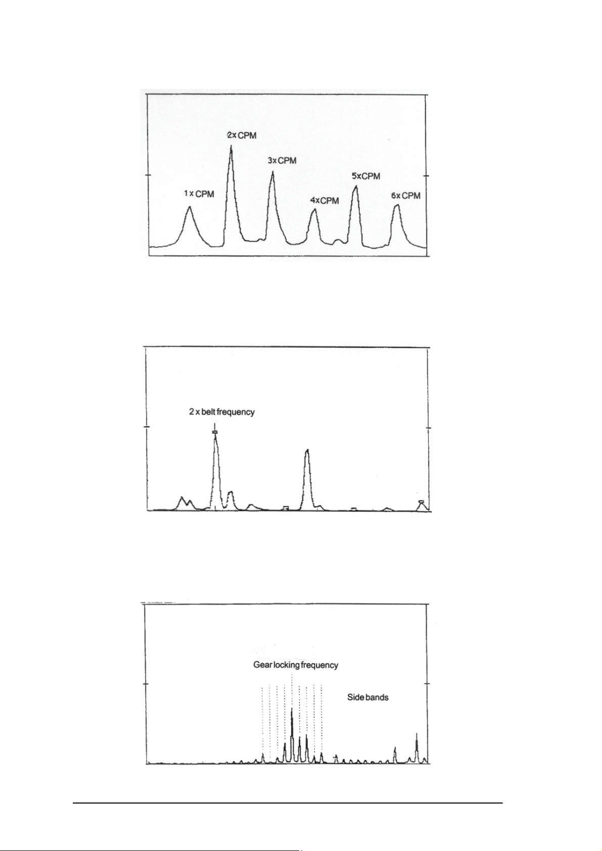
3. MECHANICAL LOOSENESS/PLAY
4. BELT
5. GEARS
C - 4 A rapid guide to interpreting a spectrum
Page 85

6. SLEEVE BEARINGS
7. ROLLER BEARINGS
8. ELECTRIC MOTORS
A rapid guide to interpreting a spectrum C - 5
Page 86

3. FORMULAE FOR CALCULATING TYPICAL BEARING DEFECT
FREQUENCIES
SYMBOLS:
FTF = housing frequency
BPFO = defect on outer track
BPFI = defect on inner track
BSP = defect on roller/ball
The frequencies of bearings can be calculated if we know:
S = number of shaft rpm
PD = primitive diameter
BD = ball/roller diameter
N = number of balls/rollers
Θ = angle of contact
The most common case:
a - fixed external ring (rotating internal ring)
BD
PD
⎛
⎜
⎜
⎝
⎛
⎜
⎝
Θ⋅
⎞
⎟
⎠
⎞
⎟
⎠
BD
PD
⎤
⎥
⎦
⎤
Θ⋅
⎥
⎦
⎤
Θ⋅
⎥
⎦
2
⎤
cos
⎞
⎟
Θ⋅
⎥
⎟
⎠
⎥
⎦
⎞
⎟
⎠
⎡
=FTF 1
⎢
2
⎣
S
N
=BPFO 1
2
S
=BPFI 1
2
PDS
⎛
⋅
=BSP
⎜
2
BD
⎝
BDS
⎞
⎛
−⋅ cos
⎟
⎜
PD
⎠
⎝
⎡
⎛
−⋅⋅ cos
⎜
⎢
⎝
⎣
⎡
BD
⎛
⋅⋅ cos
+N
⎜
⎢
PD
⎝
⎣
⎡
⎞
1
−⋅
⎢
⎟
⎠
⎢
⎣
b - rotating external ring (fixed internal ring)
BD
PD
⎛
⎜
⎜
⎝
⎛
⎜
⎝
Θ⋅
⎞
⎟
⎠
⎞
⎟
⎠
BD
PD
⎤
⎥
⎦
⎤
Θ⋅
⎥
⎦
⎤
Θ⋅
⎥
⎦
2
⎤
cos
⎞
⎟
Θ⋅
⎥
⎟
⎠
⎥
⎦
⎞
⎟
⎠
⎡
=FTF 1
⎢
2
⎣
S
N
=BPFO 1
2
S
=BPFI 1
2
PDS
⎛
⋅
=BSP
⎜
2
BD
⎝
BDS
⎞
⎛
+⋅ cos
⎟
⎜
PD
⎠
⎝
⎡
⎛
−⋅⋅ cos
⎜
⎢
⎝
⎣
⎡
BD
⎛
⋅⋅ cos
+N
⎜
⎢
PD
⎝
⎣
⎡
⎞
1
−⋅
⎢
⎟
⎠
⎢
⎣
Approximate calculation formulae (± 20%)
FTF = 0.4 x S (a) or 0.6 x S (b)
BPFO = 0.4 x N x S (a) or (b)
BPFI = 0.6 x N x S (a) or (b)
BSP = 0.23 x N x S (N < 10) (a) or (b)
= 0.18 x N x S (N ≥ 10) (a) or (b)
C - 6 A rapid guide to interpreting a spectrum
Page 87

Appendix D
Codes that can be used in models for
certificates obtained using the CEMB
PoInTer program.
When the certificate is created, the CEMB PoInTer software automatically replaces some
of the default codes in the model (#x# format) with corresponding information, related to
the measurements displayed at the time.
To ensure that they are replaced correctly, only the following codes should be used:
#1# Current date
#2# Current time
#3# Notes/comments/analyses
#4# Image of the graph (or graphs) displayed
#10# Type of graph (FFT, wave, monT, monV)
#11# Type of measurement (Pk, PP, RMS)
#50#
#51# Date/Time when Measurement 1 was taken
#52# Date/Time when Measurement 2 was taken
#53# Date/Time when Measurement 3 was taken
#101# System that measurement 1 is taken from
#102# System that measurement 2 is taken from
#103# System that measurement 3 is taken from
#151# Station that measurement 1 is taken from
Unit of measurem. for the x axis (valid for all measurements displayed)
#152# Station that measurement 2 is taken from
#153# Station that measurement 3 is taken from
#201# Machine that measurement 1 is taken from
#202# Machine that measurement 2 is taken from
#203# Machine that measurement 3 is taken from
Codes for Cemb PoInTer certificates D - 1
Page 88

#251# Point that measurement 1 is taken from
#252# Point that measurement 2 is taken from
#253# Point that measurement 3 is taken from
#301# Total (overall) value of measurement 1
#302# Total (overall) value of measurement 2
#303# Total (overall) value of measurement 1
#351# Unit of measurement for the y axis for measurement 1
#352# Unit of measurement for the y axis for measurement 2
#353# Unit of measurement for the y axis for measurement 3
#401# Frequency of peak no. 1 in graph 1
#402# Frequency of peak no. 2 in graph 1
#…# Frequency of peak no. … in graph 1
#425# Frequency of peak no. 25 in graph 1
#426# Value of peak no. 1 in graph 1
#427# Value of peak no. 2 in graph 1
#…# Value of peak no. .. in graph 1
#450# Value of peak no. 25 in graph 1
#451# Frequency of peak no. 1 in graph 2
#452# Frequency of peak no. 2 in graph 2
#…# Frequency of peak no. .. in graph 2
#475# Frequency of peak no. 25 in graph 2
#476# Value of peak no. 1 in graph 2
#477# Value of peak no. 2 in graph 2
#…# Value of peak no. .. in graph 2
#500# Value of peak no. 25 in graph 2
#501# Frequency of peak no. 1 in graph 3
#502# Frequency of peak no. 2 in graph 3
#…# Frequency of peak no. … in graph 3
#525# Frequency of peak no. 25 in graph 3
D - 2 Codes for Cemb PoInTer certificates
Page 89

#526# Value of peak no. 1 in graph 3
#527# Value of peak no. 2 in graph 3
#…# Value of peak no. .. in graph 3
#550# Value of peak no. 25 in graph 3
Codes for Cemb PoInTer certificates D - 3
 Loading...