Bio-Rad iCycler iQ Instruction manual

Download

Page 1

iCycler iQ

™

Real-Time PCR Detection System

Instruction Manual

Catalog Number

170-8740

For Technical Service Call Your Local Bio-Rad Office or in the U.S. Call 1-800-4BIORAD (1-800-424-6723)

Page 2

Safety Information

Important: Read this information carefully before using the iCycler iQ Real Time PCR Detection System.

Grounding

Always connect the iCycler Optical Module Power Supply to a 3-prong, grounded AC outlet using the AC power cord and external power supply provided with the iCycler iQ Real Time PCR Detection System. Do not use an adapter to a two-terminal outlet.

Servicing

The only user-serviceable parts of the iCycler are the lamp and filters. There are no other user-serviceable parts for this instrument. When replacing the lamp or filters, remove ONLY the outercasing of the iCycler Optical Module for lamp and filter replacement. Call

your local Bio-Rad office for all other service.

Power Switch

The external power supply must be placed so that there is free access to its power

switch.

Temperature

For normal operation the maximum ambient temperature should not exceed 30°C (see Appendix A for specifications).

There must be at least 4 inches clearance around the sides of the iCycler to adequately cool the system. Do not block the fan vents near the lamp, as this may lead to improper operation or cause physical damage to the iQ Detector.

Do not operate the iCycler Optical Module in extreme humidity (>90%) or where condensation can short internal electrical circuits or fog optical elements.

Notice

This Bio-Rad instrument is designed and certified to meet EN-61010 safety standards.

EN-61010 certified products are safe to use when operated in accordance with the instruction manual. This instrument should not be modified in any way. Alteration of this instrument will:

• Void the manufacturer’s warranty.

• Void the EN-61010 safety certification.

• Create a potential safety hazard.

Bio-Rad is not responsible for any injury or damage caused by the use of this instrument for purposes other than those for which it is intended, or by modifications of the instrument not performed by Bio-Rad or an authorized agent.

The iCycler is intended for laboratory research applications only.

Page 3

Table of Contents

Page

Section 1 Introduction ..............................................................................................1

1.1 System Description ................................................................................................2

1.2 iCycler iQ Filter Instructions ..................................................................................4

Section 2 Quick Guide to Running an Experiment ................................................6

2.1 Introduction............................................................................................................6

2.2 Quick Guide to Single or Multi-Color Experimentation .........................................6

2.3 Well Factors ...........................................................................................................8

2.4 Pure Dye Calibration and RME Files .....................................................................9

Section 3 Introduction to the iCycler Program.....................................................11

3.1 Organization of the Program ................................................................................11

3.1.1 The Library Module ...............................................................................12

3.1.2 The Workshop Module...........................................................................12

3.1.3 The Run Time Central Module...............................................................12

3.1.4 The Data Analysis Module .....................................................................13

3.2 Organization of the Manual..................................................................................13

3.3 Definitions and Conventions ................................................................................13

3.4 Thermal Cycling Parameters ................................................................................13

3.4.1 Temperature and Dwell Time Ranges.....................................................14

3.4.2 Advanced Programming Options............................................................14

Section 4 The Library Module...............................................................................15

4.1 View Protocols Window ......................................................................................15

4.2 View Plate Setup Window....................................................................................16

4.3 View Quantities and Identifiers Window..............................................................18

4.4 View Post-Run Data Window ..............................................................................19

4.4.1 Opening Stored Amplification or Melt Curve Data Files........................19

4.4.2 Opening a Stored Pure Dye Calibration File...........................................19

4.4.3 Applying a New RME File to Stored Optical Data .................................20

Section 5 The Workshop Module...........................................................................21

5.1 Edit Protocol Window ..........................................................................................21

5.1.1 Quick Quide to Creating a New Protocol................................................22

5.1.2 Quick Quide to Editing a Stored Protocol...............................................24

5.1.3 Graphical Display...................................................................................26

5.1.4 Programming Dwell Times and Temperatures in the Spreadsheet..........26

5.1.5 Editing Cycles and Steps in the Spreadsheet...........................................27

5.1.6 Select Data Collection Step(s) Box.........................................................28

5.1.7 Programming Protocol Options in the Spreadsheet.................................28

5.1.8 Saving the Protocol.................................................................................34

5.2 Edit Plate Setup Window......................................................................................34

5.2.1 Quick Guide to Creating New Plate Setup in Whole Plate Mode............37

5.2.2 Quick Guide to Editing a Stored Plate Setup in Whole Plate Mode ........38

5.2.3 Quick Guide to Creating a New Plate Setup in Dye Layer Mode............39

5.2.4 Quick Guide to Editing a Stored Plate Setup in Dye Layer Mode...........40

5.2.5 Edit Plate Setup/Samples........................................................................41

5.2.6 Select and Load Fluorphores in Whole Plate Mode ................................48

5.2.7 Select Fluorophores in Dye Layer Mode ................................................49

5.3 View Quantities and Identifiers Window..............................................................50

5.4 Run Prep Window ................................................................................................50

Page 4

5.4.1 Well Factors ...........................................................................................51

5.4.2 Pure Dye Calibration ..............................................................................55

Section 6 The Run Time Central Module .............................................................59

6.1 Thermal Cycler Window ......................................................................................59

6.1.1 Run-Time Protocol Editing.....................................................................60

6.1.2 Show Protocol Graph .............................................................................61

6.1.3 Show Plate Setup Grid............................................................................62

6.1.4 Pause/Stop ..............................................................................................62

6.2 Imaging Services..................................................................................................62

6.2.1 Description .............................................................................................63

6.2.2 Adjusting the Masks ...............................................................................64

6.2.3 Checking Mask Alignment.....................................................................65

6.2.4 Image File...............................................................................................65

Section 7 Data Analysis Module ............................................................................66

7.1 View/Save Data Window .....................................................................................66

7.1.1 View Plate ..............................................................................................67

7.1.2 Post-Run Editing ....................................................................................67

7.1.3 Saving OPD Files ...................................................................................68

7.2 PCR Quantification Window................................................................................71

7.2.1 Quick Guide to Collecting and Analyzing PCR Quantification Data......71

7.2.2 Amplification Plot ..................................................................................72

7.2.3 Amplification Plot Context Menu...........................................................72

7.2.4 PCR Quantification Data Display...........................................................79

7.2.5 Select Analysis Mode .............................................................................79

7.2.6 Select a Fluorophore...............................................................................80

7.2.7 Select Data Set........................................................................................80

7.2.8 Select Wells............................................................................................80

7.2.9 Threshold Cycle Calculation ..................................................................81

7.2.10 Save for x-axis/y-axis Allelic Analysis...................................................83

7.3 Standard Curve Window ......................................................................................83

7.4 Melt Curve Window.............................................................................................85

7.4.1 Quick Guide to Collecting and Analyzing Melt Curve Data ...................85

7.4.2 Melting Curve Plot .................................................................................85

7.4.3 Melting Curve Plot Context Menu..........................................................86

7.4.4 Melting Curve Data Spreadsheet ............................................................87

7.4.5 Select Wells............................................................................................88

7.4.6 Open/Save Settings.................................................................................88

7.4.7 Select Fluorophore..................................................................................88

7.4.8 Peak Bar .................................................................................................88

7.4.9 Temperature Bar.....................................................................................89

7.4.10 Edit Melt Peak Begin/End Temps...........................................................89

7.4.11 Delete Peaks...........................................................................................89

7.5 Allelic Discrimination Window............................................................................90

7.5.1 Quick Guide to Collecting and Analyzing Allelic Discrimination Data..90

7.5.2 Allelic Discrimination Plot .....................................................................92

7.5.3 Allelic Discrimination Plot Context Menu..............................................94

7.5.4 Allelic Data Spreadsheet.........................................................................94

7.5.5 Automatic/Manual Call ..........................................................................95

7.5.6 Display Mode .........................................................................................96

7.5.7 Vertical Threshold ..................................................................................96

7.5.8 Horizontal Threshold..............................................................................97

Page 5

7.5.9 Normalize Data ......................................................................................97

Section 8 Care and Maintenance ...........................................................................98

8.1 Cleaning the Unit .................................................................................................98

8.2 Replacing the Lamp .............................................................................................98

Appendix A Specifications ..........................................................................................99

Appendix B Minimum Computer Specifications ....................................................100

Appendix C Warranty...............................................................................................101

Appendix D Product Information.............................................................................102

Appendix E Error Messages and Alerts...................................................................103

E.1 Software Startup.................................................................................................103

E.2 Workshop and Library........................................................................................103

E.3 Run Time Central...............................................................................................107

E.4 Data Analysis .....................................................................................................110

E.5 Exiting Software.................................................................................................111

Appendix F Hardware Error Messages ...................................................................112

Appendix G Description of iCycler and iQ Data Processing...................................114

Appendix H Uploading New Versions of Firmware.................................................120

Appendix I An example Pure Dye Calibration and RME file ...............................121

Appendix J Converting from Previous Versions of iCycler iQ Software ..............123

Appendix K Melt Curve Functionality.....................................................................124

Appendix L Filter Wheel Setup and Fluorophore Selection Guide........................136

Page 6

Page 7

Section 1 Introduction

The Polymerase Chain Reaction (PCR)* has been one of the most important developments in Molecular Biology. PCR has greatly accelerated the rate of genetic discovery, making critical techniques relatively easy and reproducible.

The availability of technology for kinetic, real time measurements of a PCR in process greatly expands the benefits of the PCR reaction. Real-Time analysis of PCR enables truly quantitative analysis of template concentration. Real-Time, on-line PCR monitoring also reduces contamination opportunities and speeds time to results because traditional post PCR steps are no longer necessary. A wide range of fluorescent chemistries may be employed to monitor the PCR in progress.

The iCycler Thermal Cycler provides the optimum performance for PCR and other thermal cycling techniques. Incorporating a Peltier driven heating and cooling design results in rapid heating and cooling performance. Rigorous testing of thermal block temperature accuracy, uniformity, consistency and heating/cooling rates insure reliable and reproducible experimental results.

The iCycler iQ Real Time PCR Detection System builds on the strengths of the iCycler thermal cycling system. The iCycler iQ system features a broad spectrum light source that offers maximum flexibility in selecting fluorescent chemistries. The filter based optical design allows selection of the optimal wavelengths of light for excitation and emission, resulting in excellent sensitivity and discrimination between multiple fluorophores. The 350,000 pixel array on the CCD detector allows for simultaneous imaging of all 96 wells every second. This results in a comprehensive data set illustrating the behavior of the data during each cycle. Simultaneous image collection insures that well-to-well data may reliably be compared. The iCycler iQ system reports data on the PCR in progress in Real Time, allowing immediate feedback on reaction success. All of these features of the iCycler iQ system hardware were built to promote reliability and flexibility.

The iCycler iQ Real Time Detection System Software includes the features that make software easy and useful. The software is designed for convenience–offering speedy setup and analytical results. The functions are presented graphically to minimize hunting through menus. Tips on usage are available as your mouse glides over the buttons - and the tips can be turned off when you no longer need to see them. The iCycler software automatically analyzes the collected data at the touch of a button yet leaves room for significant optimization of results based on your analysis preferences.

Page 8

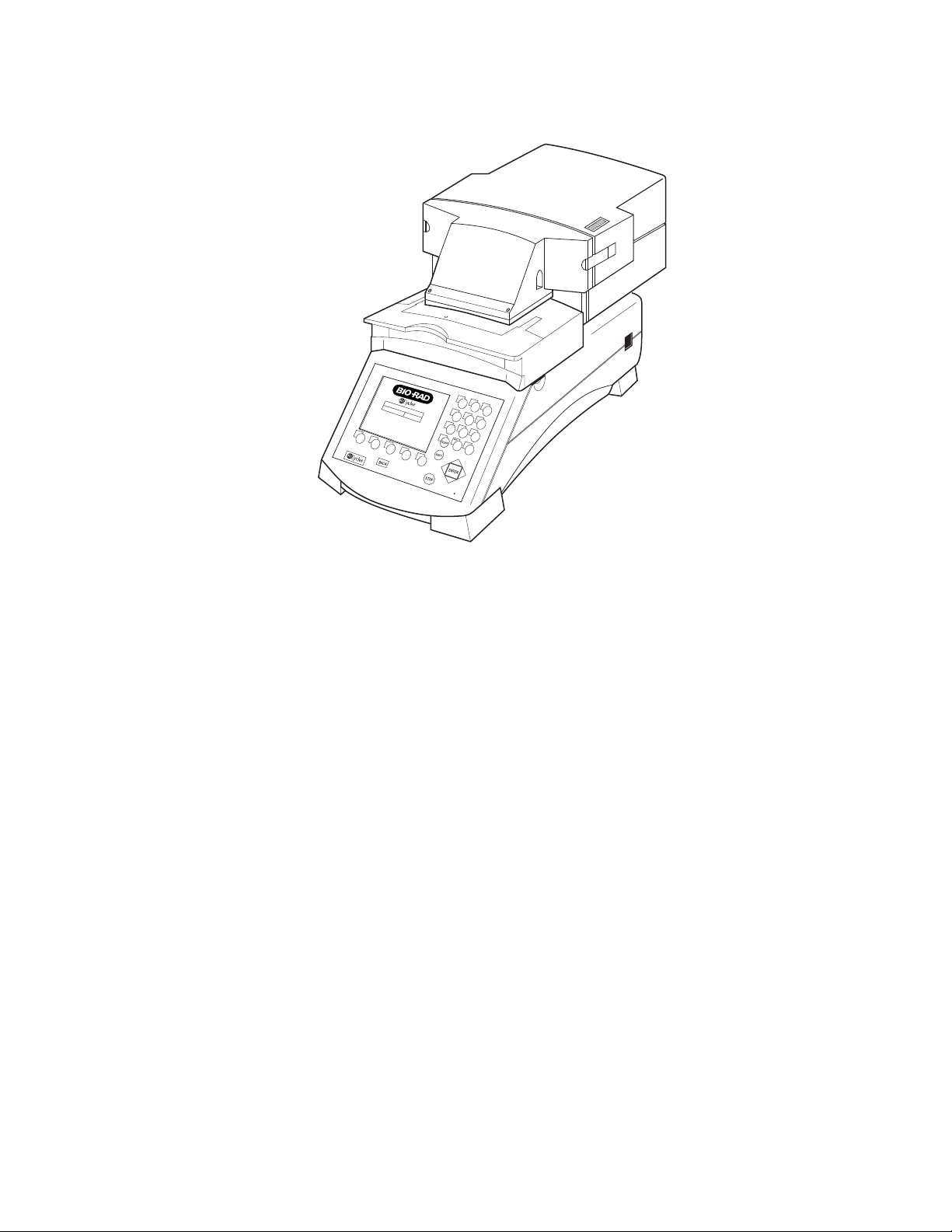
Fig. 1.1. Optical Module Upgrade to iCycler Thermal Cycler.

1.1 iCycler iQ System Description

The optical module houses the excitation system and the detection system. The Excitation system consists of a fan-cooled, 50-watt tungsten halogen lamp, a heat filter (infrared absorbing glass), a 6-position filter wheel fitted with optical filters and opaque filter “blanks”, and a dual mirror arrangement that allows simultaneous illumination of the entire sample plate. The excitation system is physically located on the right front corner of the optical module, with the lamp shining from right to left, perpendicular to the instrument axis. Light originates at the lamp, passes through the heat filter and a selected color filter, and is then reflected onto the 96 well plate in the thermal cycler by a set of mirrors. This light source excites the fluorescent molecules in the wells.

Registered User New User

er L

Page 9

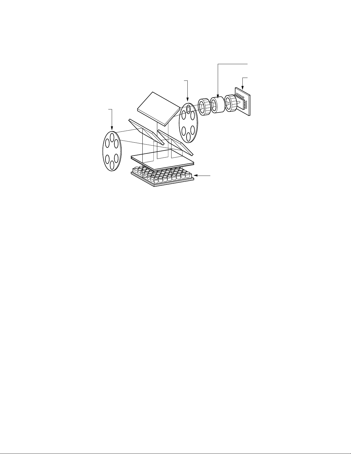
Fig. 1.2. Representation of Optical Detection System layout.

The detection system occupies the rear two-thirds of the optical module housing. The primary detection components include a 6-position emission filter wheel, an image intensifier, and a CCD detector. This filter wheel is identical to the wheel in the excitation system and is fitted with colored emission filters and opaque filter “blanks”. The intensifier increases the light intensity of the fluorescence without adding any electrical noise. The 350,000 pixel CCD allows very discrete quantitation of the fluorescence in the wells. Fluorescent light from the wells passes through the emission filter and intensifier and is then detected by the CCD.

Note: Suggested computer specifications for running the system software are given in Appendix B.

At the right side of the optical module are two connectors (see Figure 1.3):

• Round 9-pin power connector: This provides power to the optical module via

the optical system power supply. Note: Always turn power switch on the

power supply to the OFF position before connecting this connector.

• Parallel-port connector: This uses a cable that is 25 pin male-to-male and

connects to the computer. The computer requires an IEEE 1284 compatible,

8-bit bi-directional, or EPP type, parallel port. Data are transferred to the

computer via this cable.

At the right rear corner of the reaction module is a single connector.

• Miniature phone plug connector: This senses when the handle is lifted. When

the handle is lifted, the emission filter wheel shifts to the home position, blocking

light to the intensifier and the CCD detector.

At the left rear corner of the iCycler thermal cycler is a single connector.

• Serial connector: The iCycler program directs the operation of the iCycler via

this cable.

Intensifier

Emission

Filters

Excitation

Filters

Sample Plate

CCD Detector

Page 10

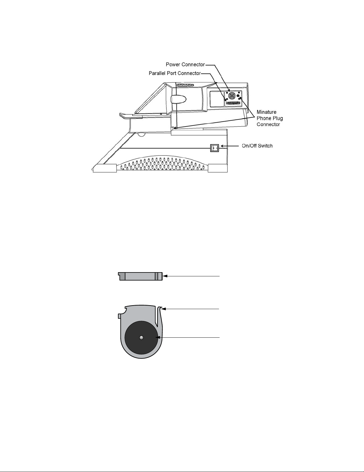
Fig. 1.3. Side View of iCycler iQ Real-Time Detection System showing cable connections.

1.2 iCycler iQ Filter Description and Instructions

Before running the iCycler program, be sure the correct filters have been installed. In addition, if the system has been moved prior to use, it is necessary to check the alignment of the mask. This procedure is discussed in Section 6.2.2. All filters are mounted in holders (see Figure 1.4). The filter holders are held in filter wheels and may be changed. Each filter wheel holds six filters. Every position in a filter wheel must have a filter or an opaque filter blank to avoid damage to the CCD detector. The first position in each filter wheel is designated as the “home” position and must always contain an opaque filter blank.

Fig. 1.4. Filter in filter holder.

To change filters, proceed as follows:

1. Turn off the power to the Optical Module.

2. Release the two black latches on each side of the Optical Module. Slide the

housing backwards 2–3” (5–8 cm), exposing a black case, the filter wheel

housing. It is not necessary to remove the housing or cables.

Tab

TOP VIEW

Tab

Filter or Filter Blank

SIDE VIEW

Page 11

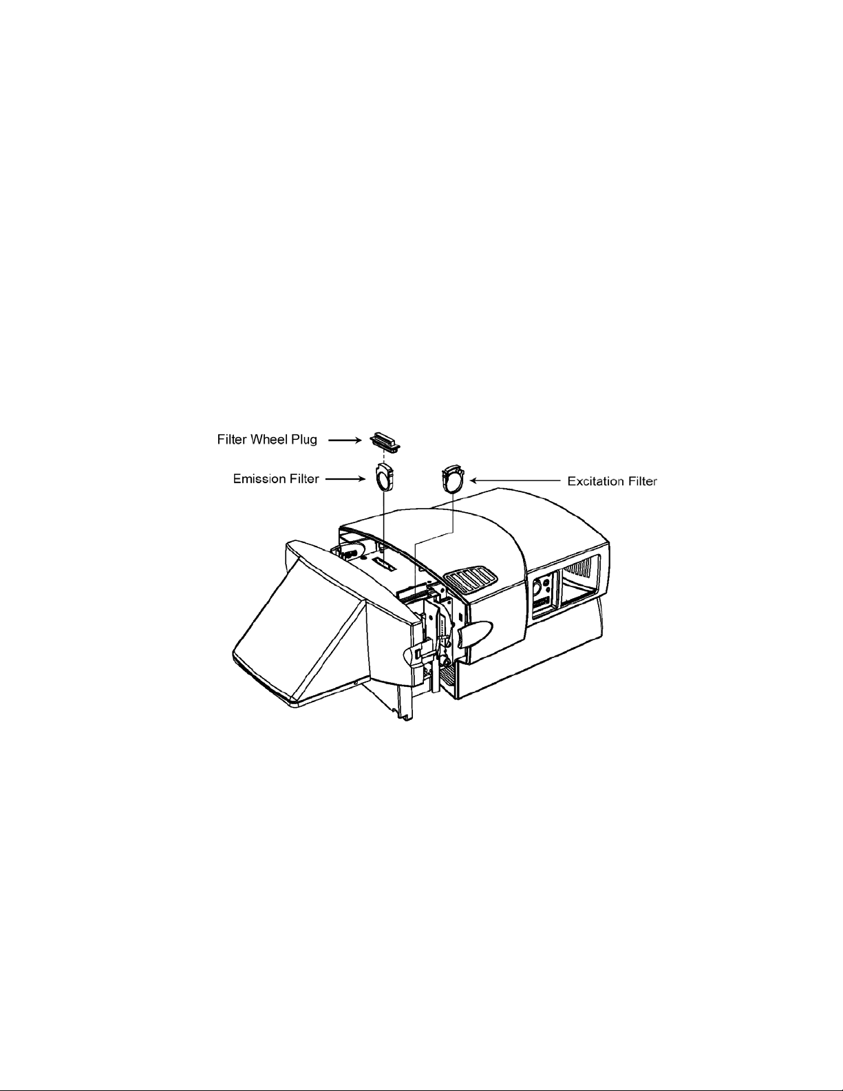
3. To access the excitation filter slot, flip open the hatch on the right side of the

instrument. To access the emission filter, remove the plug from the slot located

on top of the instrument (see Figure 1.5). Changing both types of filters is

similar.

4. Turn the filter wheels to the desired positions using the supplied ball end hex

driver. As long as the power to the Optical Module is off, the filter wheels may

be turned freely in either direction.

5. To remove a filter, grasp it on both sides with the filter removal pliers and

squeeze the tab in; gently pull the filter up and out.

6. To insert a filter, grasp the filter with the pliers and insert it into a vacant slot. For

the excitation filters, the tab on the filter is toward the front of the instrument. For

the emission filters, the tab on the filter is toward the right of the instrument. Be

sure that every position in the filter wheel has either an excitation or emission

filter or a filter blank.

Record the position of filters to compare later with the plate setup. (See

Section 5.2)

7. After the filters or filter blanks have been inserted, replace the rubber plugs

over the slots of the filter wheels.

8. Move the camera housing forward and re-attach the latches.

Fig. 1.5. Installing the filters.

Page 12

Section 2 The iCycler iQ Real Time PCR Detection System for Single and Multi-Color Experimentation

2.1 Introduction

The iCycler iQ Detector can simultaneously collect light from as many as four fluorophores in 96 wells and separate the signals into those of the individual fluorophores. This allows monitoring of up to four amplifications simultaneously on the same plate or in each well.

At each data collection step in real time, fluorescent light from each monitored well is measured through each filter pair. Since there is one filter pair for each fluorophore on the plate, each data collection step may require as many as four readings. For example, if there are probes labeled with FAM, HEX, Texas Red

and Cy™5 in a well, then at each data collection step, light from the well must be measured using the FAM filter pair, the HEX filter pair, the Texas Red filter pair and the Cy5 filter pair. The software then splits the signals into the contributions of each individual fluorophore. Using these data, separate amplification plots are displayed and at the end of the experiment, separate standard curves are automatically calculated for each fluorophore and unknown concentrations are determined on an individual fluorophore basis.

An experiment on the iCycler iQ system is defined by a Protocol file and a Plate Setup file. These files have the extensions .tmo and .pts, respectively. The output file of fluorescent data from which the amplficiation, melting curve, and standard curve data are extracted is called an Optical Data file and has the extension .opd.

In addition, every experiment on the iCycler iQ system requires well factor and pure dye calibration data in order to separate the signals of the individual fluorophores from the combined measured light. Well factors are generated for every individual experiment while pure dye calibration data persist from experiment to experiment. These two concepts are introduced below and presented in detail in Section 5.4. Understanding them will make it possible to rapidly optimize experimental protocol development and to collect the best possible optical data.

2.2 Quick Guide to Single or Multi-Color Experimentation

1. Allow the camera to warm up for 30 minutes. Power up the iCycler and log onto

the instrument. Open the iCycler software. If the iCycler or the iQ detector has

been moved since the last experiment, enter Imaging Services in the Run Time

Central module and check the alignment of the masks. See Section 6.2.

2. If necessary, conduct a Pure Dye Calibration protocol to collect the data

required to separate the signals from overlapping fluorophores. Calibration

data are required for each fluorophore/filter pair combination on the experimen-

tal plate. See Section 5.4.2.

Texas Red and SYBR are registered trademarks of Molecular Probes, Inc.

Cy is a trademark of Amersham Pharmacia Biotech.

Page 13

3. Prepare the experimental PCR reactions in a 96-well Thin Wall plate (catalog

number 223-9441). Place a sheet of Optical Quality sealing tape (catalog number

223-9444) on the top of the 96-well plate. Use the tape applicator (flat plastic

wedge) to smooth the tape surface and tightly seal the tape to the plate. Avoid

touching the surface of the sealing tape with gloved fingers. Tear off the white

strips that remain on the sides of the tape. If individual sample tubes or strips of

tubes are to be used, you must seal the tubes with the appropriate caps. Note

that a minimum of 8 sample tubes is required to prevent tube crushing when

using the green anticondensation ring. If the ring is not present, a minimum of 14

sample tubes must be present.

4. Create and save the thermal protocol in the Workshop module. The thermal

protocol specifies the dwell times and set point temperatures, the number of

cycles, steps and repeats, and the step(s) at which data collection are to occur.

See Section 5.1.

5. Create and save the Plate Setup in the Workshop module. In the Plate Setup

window, indicate what fluorophores are to be monitored in which wells and

define the sample type, and for Standards, enter the quantity and units of

measure. Check these entries in the ‘View Plate Setup’ tab before proceeding.

See Section 4.2. The process of creating the Plate Setup includes choosing the

appropriate Filter Wheel Setup file. Choose a Filter Wheel Setup that includes

all the fluorophores that you want to monitor. See Appendix L.

6. Ensure that the positions of the filters in the excitation (lamp) and emission

(camera) filter wheels are in the exact same position as defined by the filter

wheel setup chosen in Step 5. See Appendix L.

7. If you will be using an external well factor plate (see Section 2.3), place the well

factor plate in the iCycler; otherwise, place the experimental plate in the

iCycler. Click the View Protocol tab in the Library module and select the

desired Thermal Protocol; click the View Plate Setup tab in the Library module

and select the desired plate setup and then click Run.

8. In the Run Prep tab, confirm that the desired protocol and plate setup files are

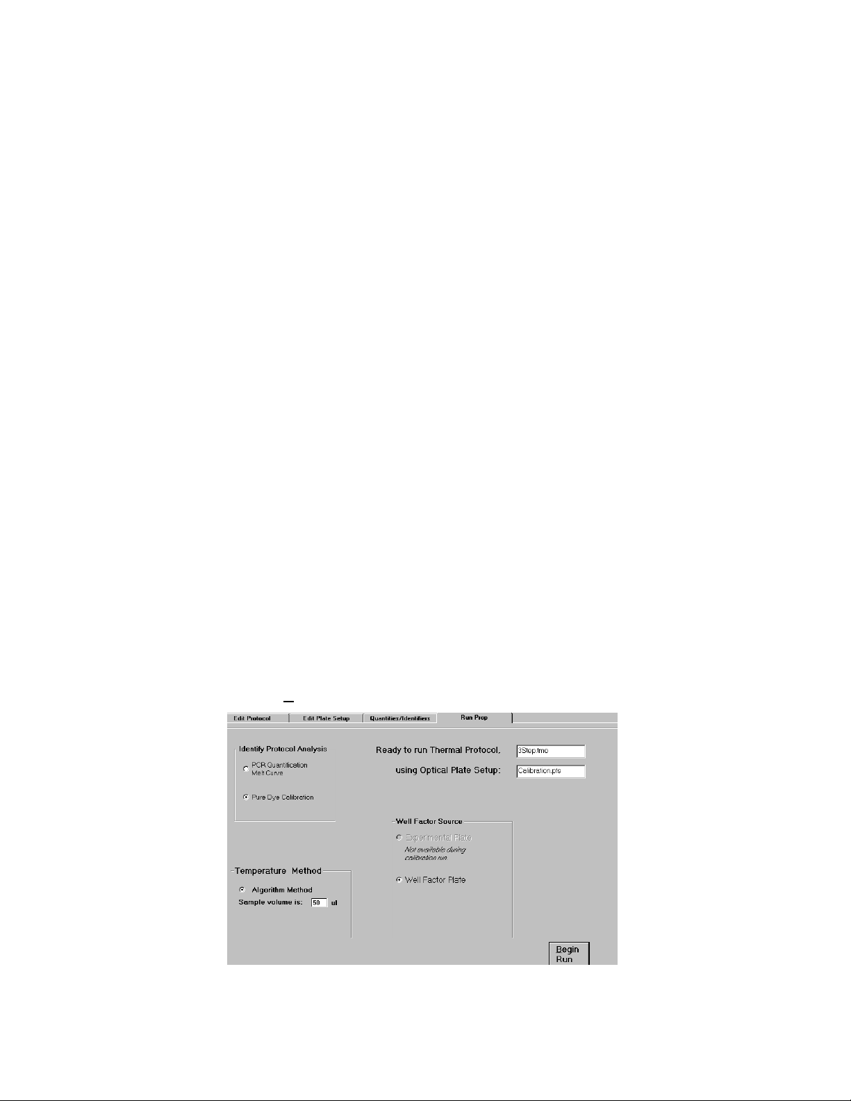
selected. Enter the reaction volume. Indicate the type of protocol (PCR

Quantification/Melt Curve or Pure Dye Calibration) and the Well Factor Source,

then click Begin Run. (Figure 2.1)

Fig. 2.1. Run prep tab.

Page 14

9. Enter a name for the data file. Data are saved during the running protocol. The

run will not begin without a data filename.

10. Well factors from the Experimental Plate will be collected automatically after you

click Begin Run and the protocol will execute immediately afterwards without

any user intervention. If you are using a Well Factor Plate, the protocol will begin

execution and after about five minutes, the external well factors will be collected

and the iCycler will go into Pause mode. During the Pause, remove the well

factor plate and replace it with the experimental plate and then click Continue

Running Protocol. (See Figure 2.6)

11. After data collection on the PCR reaction plate begins, the PCR Quantification

plot will be displayed and the software will open the Data Analysis module. It is

not possible to make adjustments to the PCR Quantification plot while data are

being collected. You can change the monitored fluorophore or adjust the size

of the plot during steps at which data are not collected.

2.3 Well Factors

Well factors are used to compensate for any system or pipetting non-uniformity in order to optimize fluorescent data quality and analysis. Well factors must be collected at the beginning of each experiment. Well factors are calculated after cycling the filter wheels through all monitored positions while collecting light from a uniform plate. Well factors may be collected directly from an experimental plate or indirectly from an external source plate.

The better and easier source of well factors is the actual experimental plate. Well factors collected from the experimental plate are called dynamic well factors. The only requirement for using dynamic well factors is that each monitored well must contain the same composition of fluorophores. Within each dye layer the fluorophore must be present at the same concentration, however, all dye layers need not have the same concentration. If all the wells on a plate have, for example, 50 nM fluorescein, 100 nM HEX, 125 nM Texas Red and 200 nM Cy5, you can use dynamic well factors because the fluorophore composition is the same in every well. If some of the wells have 100 nM fluorescein and others have 200 nM fluorescein, then you cannot use dynamic well factors and you must use external well factors. Collection of dynamic well factors is a completely automated process initiated by clicking the Experimental Plate radio button in the Run Prep screen (see Figure 2.1).

In most experiments using DNA-binding dyes like SYBR®Green I or ethidium bromide, dynamic well factors cannot be used. When the template DNA is denatured, the fluorescence of the intercalators is not sufficiently high to calculate statistically valid well factors. There are three solutions to this problem: (1) use iQ SYBR Green Supermix (Catalog # 170-8880) which already includes flourescein (2) use external well factor plate or (2) for experiments with SYBR Green I, spike the master mix with a small volume of dilute fluorescein solution (see Section 2.3.2). This dilute fluorescein results in sufficient fluorescence at 95°C so that good dynamic well factors can be calculated and it will not interfere with the PCR.

The details of preparing and using well factor plates are in the section describing the Run Prep window of the Workshop module (Section 5.4).

Page 15

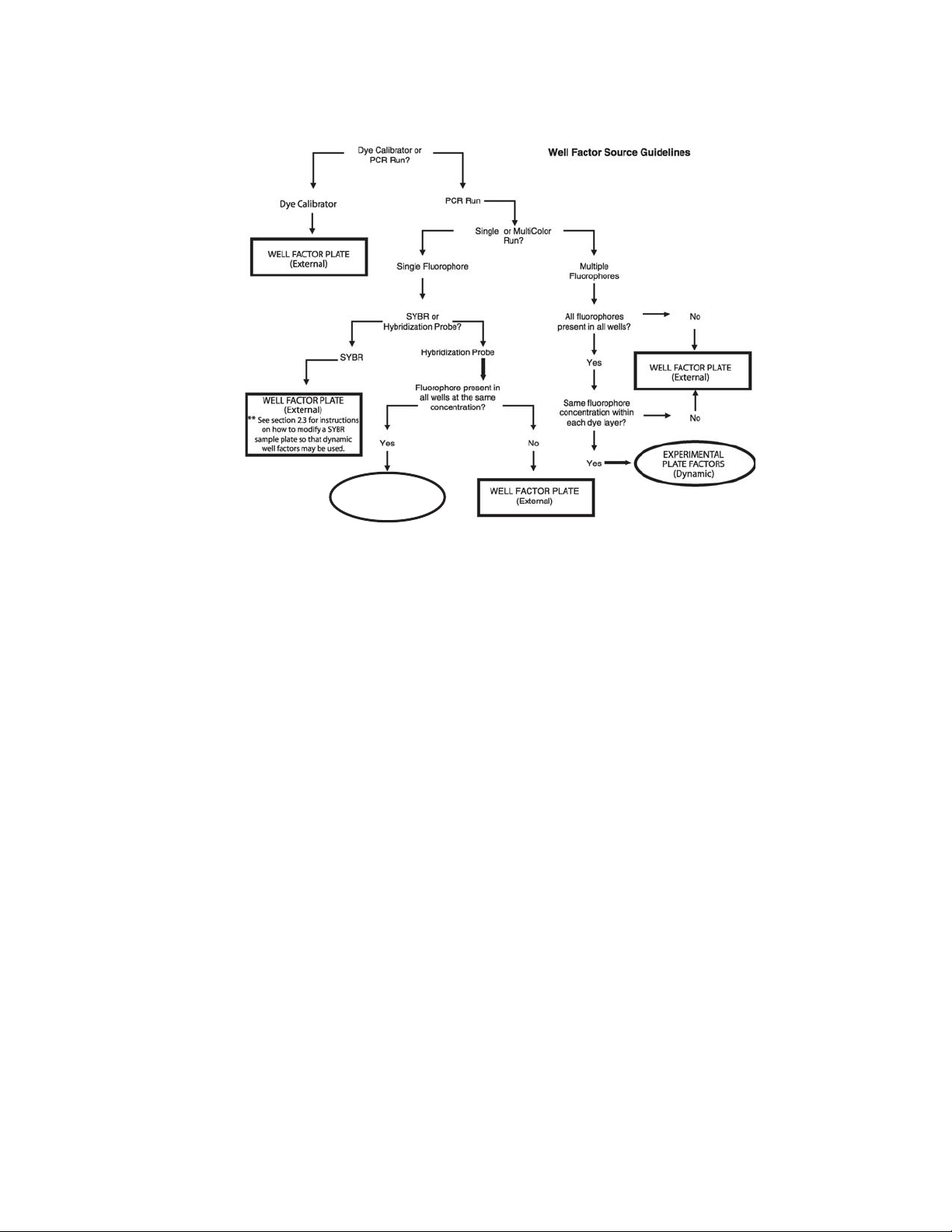
Fig. 2.2. Well Factor guidelines.

2.4 Pure Dye Calibration and RME Files

Pure dye calibration data are required for every experiment, even those that monitor only one fluorophore, however, they need not be collected at each experiment. In contrast to well factors which must be collected at the beginning of each experiment, pure dye calibration data persist from experiment to experiment. Only when a new combination of fluorophore and filter pair are added to the analysis a new pure dye calibration must be done.

The pure dye calibration data are used to separate the total light signal into the contributions of the individual fluorophores. The data are collected by executing a Pure Dye Calibration protocol on a plate containing replicate wells filled with a single pure dye calibrator solution; there is a different calibrator solution for each fluorophore. These data are written to the file RME.ini found at C:\Program Files\Bio-Rad\iCycler\Ini. Pure dye calibration data are collected on as many as 16 combinations of fluorophore and filter pairs per protocol (up to four fluorophores and up to four filter pairs). At the end of the calibration protocol, the data are automatically written to the RME file: one entry for each fluorophore/filter pair combination. Once pure dye calibration data are written to the RME file they are valid on all subsequent experiments using the same fluorophore/filter pair combinations. As more pure dye calibration protocols are executed, the RME file is updated with data for the new fluorophore/filter pair combination. If a fluorophore/filter pair combination for which an RME entry exists is repeated in a subsequent pure dye calibration protocol, the new results are written to the RME file and the old results are overwritten.

EXPERIMENTAL

PLATE FACTORS

(Dynamic)

Page 16

If a plate setup is specified that includes a fluorophore/filter pair combination for which pure dye calibration data do not exist, an alert message will be presented when the experiment is initiated. The RME file must be updated with the necessary pure dye calibration data before conducting the experiment. It is a good practice to archive RME files before running new pure dye calibration protocols. Archive the RME files by renaming them or moving them from the C:\Program Files\Bio-Rad\iCycler\Ini folder.

Every time an optical data file is created, the RME data present at the time of the experiment are saved into the file. This permits data files to be opened on other computers and also allows the original RME data to be maintained after subsequent recalibrations. It is also possible to overwrite the RME data that were used at the time of the optical data collection if the pure dye calibration data were suspect or corrupted.

There is an example of a pure dye calibration and RME file in Appendix I.

The details of preparing a pure dye calibration plate and performing the pure dye calibration are in the section describing the Run Prep window of the Workshop module (Section 5.4).

Page 17

Section 3 Introduction to the iCycler Program

3.1 Organization of the Program

The iCycler program allows you to create and run thermal cycling programs on the iCycler and to collect and analyze fluorescent data captured by the Optical Module. The operation of each instrument is controlled by separate parts of the iCycler Program. Operation of the iCycler thermal cycler is controlled by a segment of the program called ‘Protocols’. Protocol files are thermal cycling programs that direct the operation of the iCycler. The Protocol files also specify when data will be collected during the thermal cycling run. Protocol files are stored with a ‘.tmo’ extension. The details of setting up protocol files are described in Section 5.1.

Fig. 3.1 Layout of a screen.

Operation of the Optical Module is controlled by the part of the program called ‘Plate Setup’. This portion of the program allows you to specify from which sample wells data will be collected, the type of sample in each well (e.g., standard, unknown, control, etc.) and the fluorophores to be monitored. Plate setup files are stored with a ‘.pts’ extension. The details of setting up Plate Setup files are described in Section 5.2. In order to run a thermal cycling program and collect fluorescent data both a Protocol file and a Plate Setup file must be specified.

The iCycler Program is organized into four sections, called ‘modules’. These are the Library Module, the Workshop Module, the Run Time Central Module and the Data Analysis Module. Icons representing each of the modules are always shown on the left side of the screen. The module that is opened is displayed with a highlighted border while the names of the other modules have plain borders. Figure 3.1 shows the first screen you see when you open the iCycler Program: the names of all of the modules are listed on the left side of the screen with the Library Module icon highlighted, and the Library Module window is displayed on the entire right side of the screen. Each module has a different function, described below.

Page 18

3.1.1 The Library Module

The Library Module contains Protocol, Plate Setup, and Data files. In the Library you may:

• View Protocol files

• View Plate Setup files

• View Quantities and Identifiers for the Plate Setup file

• Select Data files to view in the Data Analysis Module

• Select Protocol files to edit in the Workshop Module

• Select Plate Setup files to edit in the Workshop Module

• Initiate a run using stored Protocol and Plate Setup Files

3.1.2 The Workshop Module

The Workshop Module allows you to work with Protocol and Plate Setup files. Use this module to:

• Edit existing Protocol files

• Edit existing Plate Setup files

• Create new Protocol files

• Create new Plate Setup files

• Save new and edited Protocol files

• Save new and edited Plate Setup files

• Initiate a run using new or edited Protocol and Plate Setup files.

Since Protocol and Plate Setup files are written and saved separately, you may “mix and match” a different file from each category in new experiments.

3.1.3 The Run Time Central Module

Once settings are confirmed in the Run Prep section of the Workshop Module, the iCycler Program transfers you directly into the Run Time Central Module where you may monitor the progress of the reaction, including the start and completion time for the experiment, the current cycle, step, and repeat number and the thermal activity of the iCycler thermal cycler.

Page 19

3.1.4 The Data Analysis Module

This module may be accessed in either of two ways.

1. It opens automatically from the Run Time Central Module when the iCycler iQ

Real Time PCR Detection System begins collecting fluorescence data which

are being analyzed in real time. This allows you to monitor a reaction as it

occurs.

2. You may open a stored data set from the Library Module and the data will

automatically be presented in the Data Analysis Module.

This module allows you to:

• View experimental data

• Optimize data

• Assign threshold cycles for all standards and unknowns

• Construct standard curves

• Determine starting concentrations of unknowns

• Conduct statistical analyses.

3.2 Organization of the Manual

The four sections that follow this one describe each of the four modules. Within each section, the manual is organized by the separate windows of the module.

3.3 Definitions and Conventions

The following customs have been adopted in the text of this instruction manual:

• A “window” refers to the view of the iCycler Program found on the computer

screen.

• Active buttons across the top of a window are referred to as ‘tabs’.

• A text box refers to a field in the window that you can type in.

• A field box refers to a region in the window that you cannot type in but provides

information about the program.

• A dialog box refers to a region in the window that allows you to make a selection.

• All active buttons are printed in bold type in the text descriptions and figure

legends. For example, the Edit button is always printed in bold since selecting

this will result in some action by the iCycler Program.

3.4 Thermal Cycling Parameters

Protocol files contain the information necessary to direct the operation of the iCycler. A protocol is made up of as many as nine cycles, and a cycle is made up of as many as nine steps. A step is defined by specifying a setpoint temperature and the dwell time at that temperature. A cycle is defined by specifying the times and temperatures for all steps and the number of times the cycle is repeated. Cycles may be repeated up to 600 times.

Page 20

3.4.1 Temperature and Dwell Time Ranges

Temperatures between 4.0 and 100.0 °C may be entered for any setpoint temperature.

Finite dwell times may be as long as 99 minutes and 59 seconds (99:59) or as short as 1 second (00:01).

Zero Dwell Times. When the dwell time is set to 00:00, the iCycler will heat or cool until it attains the setpoint temperature and then immediately begin heating or cooling to the next setpoint temperature.

3.4.2 Programming Options

Many advanced options are available for thermal protocols. They are listed below and detailed in the section describing the Edit Protocol window of the Workshop (Section 5.1).

• Infinite Hold. Holds a defined temperature indefinitely until user intervention.

• Gradient. Allows a reproducible gradient of between 1 and 25 C to be

programmed down-the-block during any single step.

• Melt Curve. Enables collection of data over a specified temperature range to

collect melting curve data for analysis.

• Increment/Decrement Temperature. Defines a periodic incremental increase

or decrease in temperature during a repeated cycle.

• Increment/Decrement Time. Defines a periodic incremental increase or

decrease in dwell time during a repeated cycle.

• Ramping. Allows specification of the rate of heating and cooling.

• Cycle Description. Names the cycles of the protocol.

• Step Process. Names the steps of a cycle.

Page 21

Section 4 The Library Module

From the Library module you may initiate experiments using saved protocol and plate setup files, view saved Protocols and Plate Setup files and open saved Optical Data files. The Quantities and Identifiers of the currently selected plate setup file and any notations about the currently selected optical data file are also available in the Library. Protocol and plate setup files viewed in the Library may be selected for editing in the Workshop or you may choose to create a new protocol or plate setup in the Workshop.

The Library module consists of four windows; each is accessed by its associated tab.

• View Protocol: Allows navigation of stored protocol files. Provides information

on the thermal parameters for the protocol specified and indicates when data

will be collected and analyzed (see Figure 4.1).

• View Plate Setup: Allows navigation of stored plate setup files. Provides

information about the location of sample wells, the sample type and the

fluorophores that will be analyzed in each (see Figures 4.2 and 4.3).

• View Quantities and Identifiers: Displays information entered by the user

when the plate setup was created (see Figure 4.4).

• View Post-Run Data: Allows navigation of stored data files. Displays any

notes entered by user. Permits opening of stored data files (see Figure 4.5).

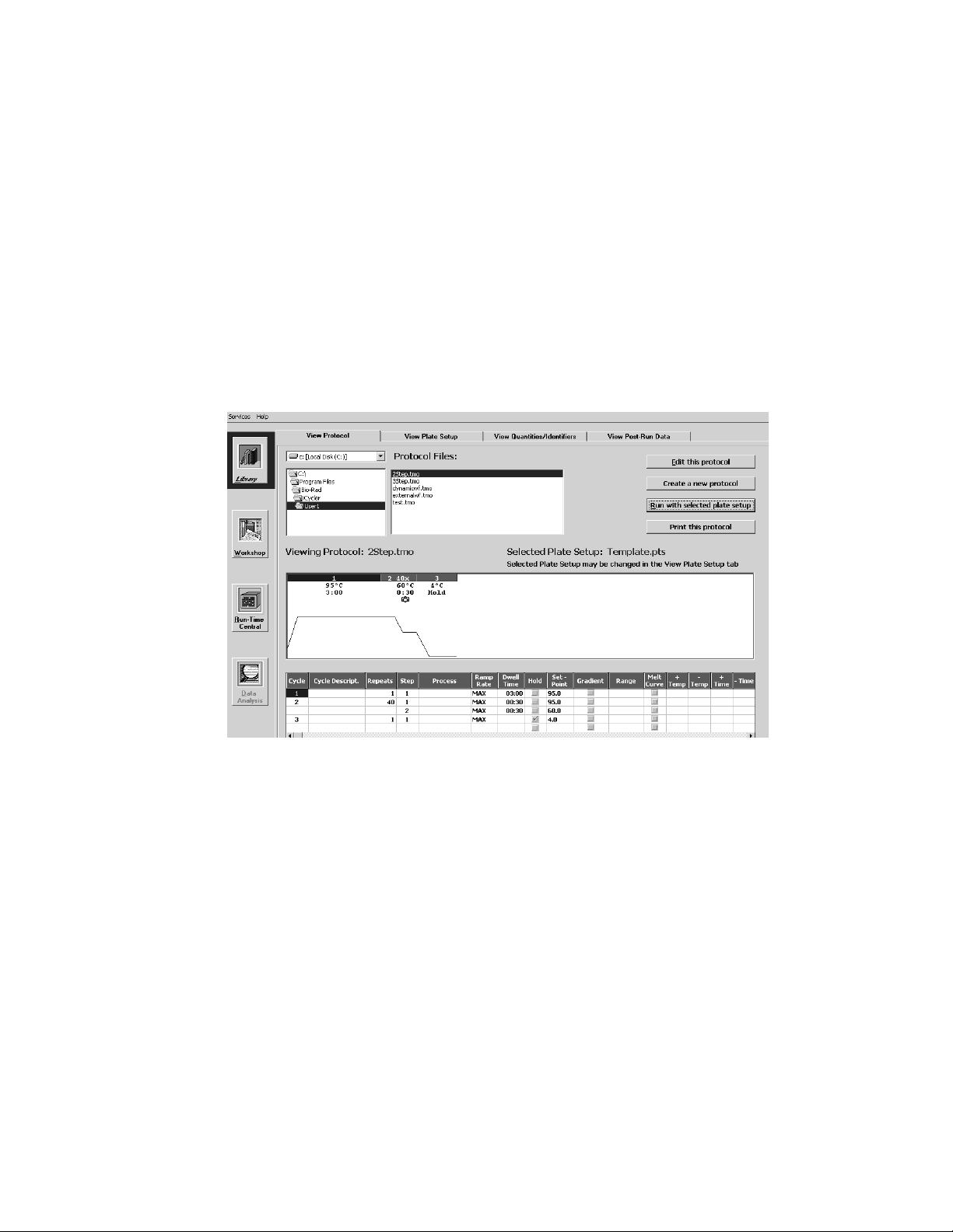
4.1 View Protocol Window

The View Protocol window of the Library module is the first window that appears when the iCycler program is opened (see Figure 4.1). In this window, you can navigate the directory of protocol files. When a protocol file name is highlighted in the directory tree, the details of the protocol are displayed in the View Protocol window.

The lower half of the window displays the protocol file identified in the Viewing Protocol field both graphically and in spreadsheet format (see Figure 4.1). The graphical display shows the reaction temperature (on the y-axis) as a function of time (on the x-axis). In the graphical display:

• The bar across the top of the graphical display shows the cycle number;

• The numbers below the bar indicate the setpoint temperature for each step in

the cycle (i.e., the y-axis on the graph) and the dwell time specified for that step

(i.e., the x-axis on the graph).

• The presence of a camera icon on a particular cycle of the graphical display

indicates that optical data will be collected at that step. A yellow camera icon

indicates that amplification data will be collected while a green camera icon

indicates collection of melt curve data.

Details of specialized options, such as automatic increment and decrement of temperature or dwell time are provided in the spreadsheet but not in the graphical display.

Page 22

Fig. 4.1. Library / View Protocol Window. This is the default window that appears upon opening the

iCycler Program.

The upper part of the window displays the following protocol file information.

• The Drive Location: The Protocol files shown here are stored on the C drive.

• The Directory Tree: The Protocol files shown here are stored in the User1 folder.

• The Protocol Files menu: A list box of all protocol file names in the directory

identified in the Directory Tree. All protocol filenames have a .tmo extension.

• The Viewing Protocol field box: The file name of the protocol displayed in this

window.

• The Selected Plate Setup field box: The currently loaded plate setup file.

The right side of the window has the following active buttons.

• E

dit this protocol: Transfers the selected Protocol file to the Edit Protocol

window of the Workshop; this allows you to edit the protocol displayed on the

screen.

• Create a new protocol: Transfers to the Edit Protocol window of the

Workshop for creation of a new protocol file.

• Run with selected plate set up: Transfers the selected protocol file and the

selected plate setup file to the Run Prep window of the Workshop for initiation

of an experiment.

• Print this protocol: Prints the spreadsheet section of the selected Protocol.

4.2 View Plate Setup Window

In this window, you can navigate the directory of plate setup files. When a plate setup file name is highlighted in the directory tree, the details of the plate setup, including the monitored wells, the sample types loaded in each well and the fluorophores loaded in each well, are displayed in the View Plate Setup window (Figure 4.2).

Page 23

Fig. 4.2. Library / View Plate Setup Window, Fluors and Samples, Show All Fluors View.

The upper part of the View Plate Setup window is similar to the upper part of the View Protocol window (compare Figures 4.1 and 4.2.)

The View Plate Setup window displays the following plate setup file information:

• The Drive Location: Plate setup files are stored on the C drive.

• The Directory Tree: The directory location of the current plate setup; plate

setup files are stored in the User1 folder.

• The Plate Setup Files menu: A list box of all plate setup file names in the

directory identified in the Directory Tree; all plate setup filenames have a .pts

extension.

• The Viewing Plate Setup field: The filename of the plate setup displayed in this

window

• The Selected Protocol field: The filename of the currently selected protocol file.

The View Plate Setup window has the following active buttons:

• Edit

this plate setup: Transfers the selected Plate Setup file to the Edit Plate Setup window of the Workshop; this allows you to edit the plate setup displayed on the screen.

• Create a new plate setup: Transfers to the Edit Plate Setup window of the Workshop; this allows you to create a new plate setup beginning with a blank plate layout.

• Run

with selected protocol: Transfers the selected plate setup file and the currently selected protocol file to the Run Prep window of the Workshop for initiation of an experiment.

There are two buttons above the sample plate grid.

Page 24

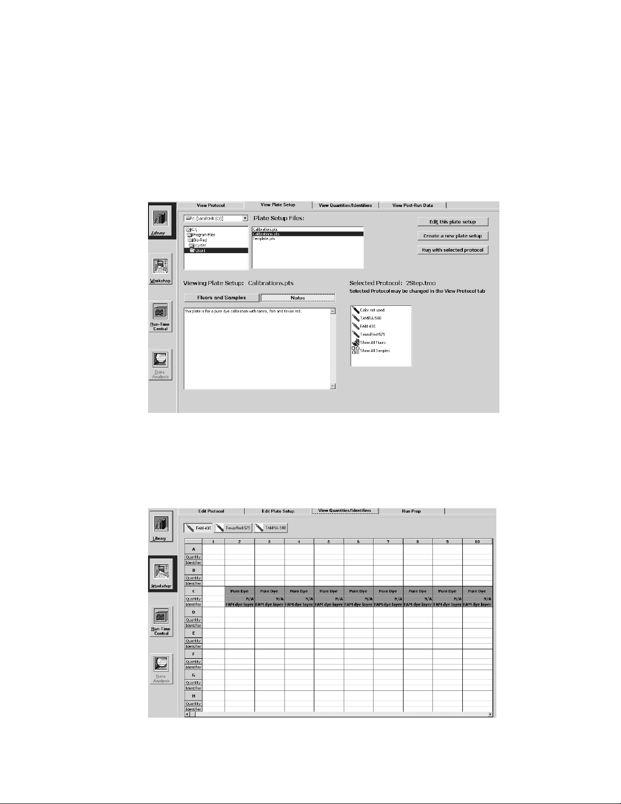
• Fluors and Samples. A list of all fluorophores defined for the selected plate setup file is displayed in the box on the right. When one of these fluorophore names is highlighted, the corresponding sample type for each well containing that fluorophore is displayed on the grid. When Show All Fluors is selected, then the wells of the grid are filled with the corresponding color of each fluorophore monitored in that well. When Show All Samples is selected then the wells of the grid are filled with the appropriate sample type icons.

• Notes: Displays any notes written about the plate setup (see Figure 4.3).

Fig. 4.3. Library / View Plate Setup window, Notes view.

4.3 View Quantities and Identifiers Window

This window displays standard quantities and identifiers for every well of the

plate setup currently selected in the View Plate Setup Window. Data are displayed one dye layer at a time.

Fig. 4.4. Library / View Quantities/Identifiers window.

Page 25

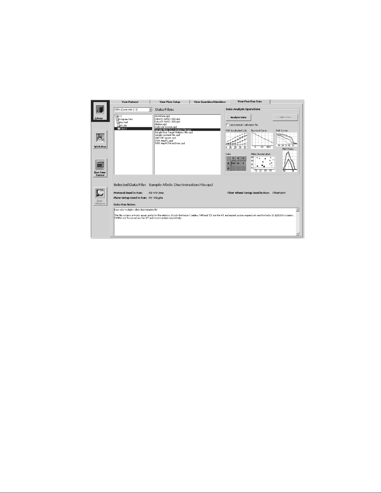
4.4 View Post-Run Data Window

The View Post-Run Data window is used to navigate the directory tree of opti-

cal data files. When an optical data file name is highlighted, the following information is displayed:

Fig. 4.5. Library / View Post-Run Data Window.

• The name of the optical data file is shown in the Selected Data File field box:.

• The protocol used.

• The plate setup used.

• Data Run Notes: These are notes entered by the user at the time of the run.

• The Filter Wheel Setup used in the experiment.

4.4.1 Opening Stored Amplification or Melt Curve Data Files

To open an optical data file from an amplification or melt curve experiment,

select its name in the directory tree and click Analyze Data.

4.4.2 Opening a Stored Pure Dye Calibration File

If the selected optical data file is a pure dye calibration file, then the

Calibration button will be active. Click this button to open the pure dye calibration optical data file. Note: opening a stored pure dye calibration optical data file

will cause the current RME file to be overwritten with the data in the selected pure dye calibration file. All subsequent experimental data will be collected and

analyzed with the new RME file. See the discussion on Pure Dye Calibration and RME files in Section 5.4 and Appendix I.

Page 26

4.4.3 Applying a New RME File to Stored Optical Data

When an optical data file is saved, the RME values are written to the file along

with the collected experimental data making it possible to analyze the data on a computer without RME data or a computer with different RME data. Any time that the optical data file is subsequently opened with the iCycler program, the data are analyzed using the values that were in the RME.ini file when the optical data were collected. It is possible to overwrite the RME values stored within the OPD file with the ones in the current RME.ini file, thus changing the analysis of the experimental data. This feature protects you from losing valuable experimental data if a pure dye calibration was conducted incorrectly.

Fig. 4.6. Enabling external calibration file option.

In order to apply the current RME values to a stored data set, highlight the

name of the optical data file in the directory tree and then click the box labeled Use External Calibration File. The optical data file will be opened and the new RME values will be applied to the data. The existing RME values will be overwritten if you save the file again. If the software is exited without explicitly saving the data set again the original RME values will be restored. Optical data may be analyzed repeatedly with different RME files simply by exchanging the location of stored (inactive) RME files with the active RME file. The only active RME file is the one stored at C:\Program Files\Bio-Rad\iCycler\Ini.

Note: It is recommended that the optical data file is saved under a different name before saving the file with new RME values. This ensures that the original file is always maintained for reference.

Page 27

Section 5 The Workshop Module

The Workshop module is where Protocol and Plate Setup files are edited

and created. Section 5.1 describes the layout of the Edit Protocol window and instructions for creating and editing protocol files. Section 5.2 describes the organization of the Edit Plate Setup window and explains how to create and edit plate setup files.

There are four windows in the Workshop:

• Edit Protocol: Protocol files are created, edited and saved in this window. You can initiate an experiment with the displayed protocol, once it is saved, and the currently loaded plate setup from this window.

• Edit Plate Setup. Plate setup files are created, edited and saved in this win- dow. You can initiate an experiment with the displayed plate setup, once it is saved, and the currently loaded protocol from this window.

• View Quantities/Identifiers: This window displays information entered in the Edit Plate setup window on an individual dye-layer basis.

• Run Prep: When you choose to run a protocol or plate setup from either the Workshop or the Library, this is window in which you confirm the protocol file, plate setup file, and conditions for the run. The experiment begins when you click Begin Run in this window.

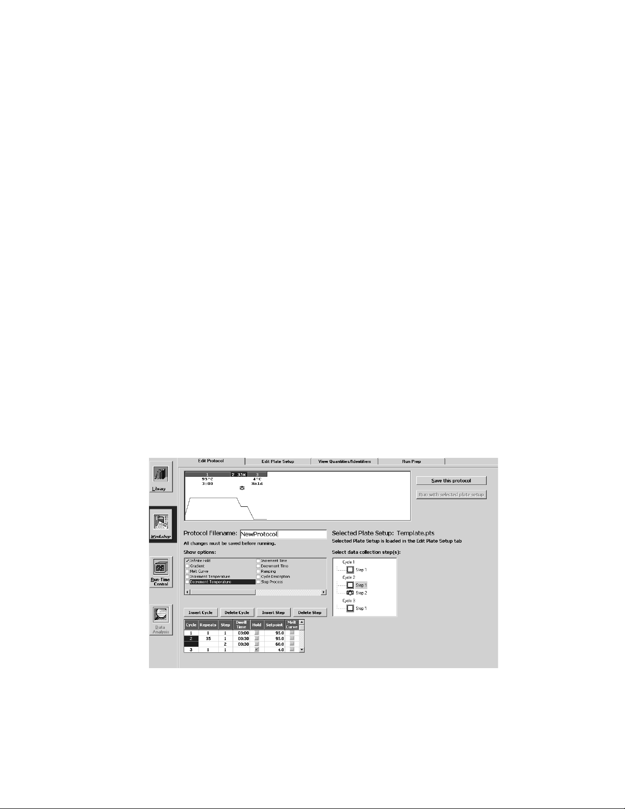
5.1 Edit Protocol Window

New protocols are created and existing protocols are edited in the Edit Protocol

window. (Figure 5.1)

Fig. 5.1. Workshop / Edit Protocol Window. This shows the minimum programming spreadsheet.

Page 28

A graphical display of the currently loaded protocol, showing reaction temperatures

(on the y-axis) and dwell times (on the x-axis), is shown in the middle one-third of the window. The actual thermal protocol is displayed in an adjustable spreadsheet at the bottom of the window.

This window contains:

• The Show options box lists advanced options that can be applied to the protocol (see below).

• The Protocol Filename text box contains the protocol filename.

• The Save this Protocol and Run with selected plate setup buttons are used to save changes to the protocol and to run the protocol, respectively (see Sections 5.1.8 and 5.4);

• The Select data collection step(s) box may be used to specify the step at which the data are collected. This is described below.

The procedures for creating new protocols and editing existing ones are

summarized in Sections 5.1.1 and 5.1.2. The graphical display is described in Section 5.1.3. Programming in the spreadsheet and specifying optical data collection are described in detail in Sections 5.1.4–5.1.7, and the saving of protocol files is detailed in Section 5.1.8.

5.1.1 Quick Guide to Creating a New Protocol

1. From the Library module, select the View Protocol tab.

2. Click Create a new protocol. The Edit Protocol window of the Workshop module will open.

3. Start in the spreadsheet at the bottom left of the window and fill in the thermal cycling protocol. As you make changes in the spreadsheet, they are reflected in the graphical representation at the top of the window. The cycle being edited is shown in blue on the bar across the top of the graph and is highlighted in blue in the spreadsheet.

• Double click in a time or temperature field to change the default settings.

• Insert a new cycle in front of the current cycle by clicking Insert Cycle and

then clicking anywhere on the current cycle in the spreadsheet. Insert a cycle after the last cycle by clicking Insert Cycle and then clicking anywhere on the first blank line at the bottom of the spreadsheet. If you right mouse click on the Insert Cycle button, you can choose to insert a 1-, 2- or 3-step cycle. When finished, deselect Insert Cycle.

• Delete cycles by clicking Delete Cycle and then clicking anywhere on that

cycle in the spreadsheet. When finished, deselect Delete Cycle.

• Insert a step in front of the current step by clicking Insert Step and then clicking

on the current step. If you right mouse click on the Insert Step button, you can choose to insert the new step before or after the current step. When finished, deselect Insert Step.

• Delete steps by clicking Delete Step and then clicking anywhere on the

line containing the step to be deleted. When finished, deselect Delete

Step.

Page 29

4. If you want to add any protocol options, first enable them by clicking in the check box next to its description in the Show options box.

• Infinite Hold. A column labeled Hold will appear in the spreadsheet. Click

the Hold button on any step of a non-repeated cycle and the set point temperature will be maintained indefinitely until user intervention. A red check mark will appear in the Hold column of the spreadsheet. Turn off the Hold by clicking on the red check mark. The software will not allow you to program a Hold if the cycle is repeated.

• Gradient. Two new columns appear in the spreadsheet. Click the Gradient

button on the desired step. Specify the range of the gradient in the other column. The range may be from 1° to 25°C across the block and the block temperatures must be in the range of 40° to 95°C.

• Melt Curve. Three new columns appear in the spreadsheet. Click the Melt

Curve column on the step at which melt curve data are to be collected. Indicate the temperature increment or decrement with each cycle. A green camera will appear on the corresponding step in the Select Data Collection Step box.

• Increment Temperature /Decrement Temperature. Three new columns will

appear. Specify the increment or decrement in temperature, the first cycle at which the change is to occur and the frequency with which the change is to occur. For example, to increase temperature by 0.2°C beginning with the third cycle and to further increase the temperature every other cycle after that you would enter 0.2 in the + Temp column, 3 in the Begin Repeat column and 2 in the How Often column.

• Increment Time /Decrement Time. Three new columns will appear.

Specify the increment or decrement in time, the first cycle at which the change is to occur and the frequency with which the change is to occur. For example, to decrease time by 2 seconds beginning with the third cycle and to further decrease the time every other cycle after that, you would enter 00:02 in the - Time column, 3 in the Begin Repeat column and 2 in the How Often column.

• Ramping. Double click in the Ramping column and choose MIN or MAX

or make a direct entry of heating or cooling rate. Valid entries are from

0.1° to 3.3°C/sec for heating steps and 0.1° to 2.0°C/sec for cooling steps.

• Cycle Description/Step Process. One new column appears if either of

these is selected. Choose a descriptive name from the pull down menu or enter one directly.

5. In the Select data collection step(s) box, specify the cycles at which fluores- cent data are to be collected for quantitative experiments.

• Click once in a camera square to indicate that data are to be collected for

post-run analysis. A camera with a yellow lens will appear in the box and on the graphical display.

• Click a second time to indicate that fluorescent data are to be collected

and analyzed in real time. REAL TIME will appear next to the yellow camera in the Select data collection step(s) box.

Page 30

• Click a third time to deselect data collection for that cycle. The camera

icon will disappear.

6. Double click in the Protocol File Name text box and enter a new name for the protocol.

7. Click Save this protocol. A Save dialog box will appear, click Save again.

Note: You may save plate setup and protocol files to the iCycler folder or any subfolder of the iCycler folder.

5.1.2 Quick Guide to Editing a Stored Protocol

1. From the Library module, select the View Protocol tab.

2. In the top left corner of the window, select the drive where the stored plate setup file resides.

3. Use the directory tree to locate the folder containing the stored protocol file.

4. Select the desired file from the Protocol Files box.

5. Click Edit this protocol. The Edit Protocol window of the Workshop module will open.

6. Start in the spreadsheet at the bottom left of the window and fill in the thermal cycling protocol. As you make changes in the spreadsheet, they are reflected in the graphical representation at the top of the window. The current cycle begin edited is shown in blue on the bar across the top of the graph and is highlighted in blue in the spreadsheet.

• Double click in a time or temperature field to change the settings.

• Insert a new cycle in front of the current cycle by clicking Insert Cycle and

then clicking anywhere on the current cycle in the spreadsheet. Insert a cycle after the last cycle by clicking Insert Cycle and then clicking anywhere on the first blank line at the bottom of the spreadsheet. If you right mouse click on the Insert Cycle button, you can choose to insert a One-, Two- or three-step cycle. When finished, deselect Insert Cycle.

• Delete cycles by clicking Delete Cycle and then clicking anywhere on that

cycle in the spreadsheet. When finished, deselect Delete Cycle.

• Insert a step in front of the current step by clicking Insert Step and then

clicking on the current step. If you right mouse click on the Insert Step button, you can choose to insert the new step after the current step. When finished, deselect Insert Step.

• Delete steps by clicking Delete Step and then clicking anywhere on the

line containing the step to be deleted. When finished, deselect Delete Step.

7. If you want to add any protocol options, choose them by clicking in the check box next to its description in the Show options box.

• Infinite Hold. A column labeled Hold will appear in the spreadsheet. Click the

Hold button on any step of a non-repeated cycle and the set point temperature will be maintained indefinitely until user intervention. A red check mark will appear in the Hold column of the spreadsheet. Turn off the Hold by clicking on the red check mark. The software will not allow you to program a Hold if the cycle is repeated.

Page 31

• Gradient. Two new columns appear in the spreadsheet. Click the

Gradient button on the desired step. Specify the range of the gradient in the other column. The range may be from 1° to 25°C across the block and the block temperatures must be in the range of 40° to 95°C.

• Melt Curve. Three new columns appear in the spreadsheet. Click the Melt

• Increment Temperature /Decrement Temperature. Three new columns

will appear. Specify the increment or decrement in temperature, the first cycle at which the change is to occur and the frequency with which the change is to occur. For example, to increase temperature by 0.2°C beginning with the third cycle and to further increase the temperature every other cycle after that you would enter 0.2 in the + Temp column, 3 in the Begin Repeat column and 2 in the How Often column.

• Increment Time /Decrement Time. Three new columns will appear.

• Ramping. Double click in the Ramping column and choose MIN or MAX

or make a direct entry of heating or cooling rate. Valid entries are from 0.1° to 3.3°C/sec for heating steps and 0.1° to 2.0°C/sec for cooling steps.

• Cycle Description/Step Process. One new column appears if either of

these is selected. Choose a descriptive name from the pull down menu or enter one directly.

8. In the Select data collection step(s) box, specify the cycles at which fluorescent data are to be collected for quantitative experiments.

• Click once in a camera square to indicate that data are to be collected for

post-run analysis. A camera with a yellow lens will appear in the box and on the graphical display.

• Click a second time to indicate that fluorescent data are to be collected

and analyzed in real time. REAL TIME will appear next to the yellow camera in the Select data collection step(s) box.

• Click a third time to deselect data collection for that cycle. The camera

icon will disappear.

9. If you want to write over your old protocol, click Save this protocol.

10. If you want to rename your protocol, double click in the Protocol Filename text box and enter a new name for the protocol and click Save this protocol. A Save dialog box will appear, click Save again.

Note: You may save the plate setup and protocol files to the iCycler folder or any subfolder of the iCycler folder.

Page 32

5.1.3 Graphical Display

The graph at the top of the Edit Protocol window shows a pictorial display of the

temperature cycling program (Figure 5.1). The bar above the graphical display indicates the cycle number for each section of the protocol; the active cycle (i.e., the one being edited) is highlighted. The setpoint temperature and the dwell time for each step are displayed below the bar. Note that occasionally space limitations do not permit display of all temperature and time settings.

You can expand the time axis in the graphical display by holding down the Ctrl

key while dragging the cursor over a section of the graph. When the left mouse button is released, the time axis will expand. Use the scroll bar at the bottom of the graph to move across the time axis of the graph. To zoom out, place the cursor anywhere in the area of the graph and click the left mouse button.

When optical data collection is specified (see Figure 5.1 and Section 5.1.6), a

camera icon is shown below the temperature at the step(s) the data will be collected. A camera icon with a yellow lens indicates that quantitative data will be collected while a camera icon with a green lens indicates that optical data will be collected for melt curve analysis.

Placing the cursor anywhere over the graphical display and pressing the right

mouse button displays the following menu:

Fig. 5.2. Context menu for protocol graph.

• Copy Graph: allows you to copy the graph to the clipboard so that it can be pasted to another application such as a text or a spreadsheet program.

• Print Graph: allows you to print a copy of the graph.

5.1.4 Programming Dwell Times and Temperature in the Spreadsheet

The bottom third of the Workshop / Edit Protocol window displays a spreadsheet

that shows each cycle and step in the protocol. There are five columns which are always present and which must be specified for any protocol. These are:

Fig. 5.3. Protocol spreadsheet.

• Cycle: a group of up to 9 steps (numbered 1–9) that are repeated; there may be up to 9 cycles (numbered 1 to 9) in a protocol;

• Repeats: the number of times a cycle is repeated; cycles may be repeated up to 600 times; the repeat number is displayed only for the first step of a multi-step cycle.

Page 33

• Step: an individual temperature or dwell time event; each cycle may have up to 9 steps;

• Dwell time: the time the step is maintained at the specified temperature; this may vary from 1 sec (0:01) to 99 min, 59 sec (99:59);

• Setpoint: the specified temperature that the reaction step will achieve; this may be with-in the range of 4.0° to 100.0°C.

5.1.5 Editing Cycles and Steps in the Spreadsheet

Fig. 5.4. Insert/delete cycles or steps.

Cycles and Steps in the thermocycling program may be inserted and deleted

using the Insert Cycle, Insert Step, Delete Cycle, and Delete Step buttons above the spreadsheet. A new cycle may consist of one, two, or three steps.

• To insert a cycle:

a. Right mouse click Insert Cycle and an active box will appear showing

1-step, 2-step, and 3-step. (Note, a one-step cycle is the default setting.)

b. Select the appropriate number of steps; the active box will disappear and

the Insert Cycle button will be highlighted.

c. In the spreadsheet, select a cell within a cycle that will follow the inserted

cycle; a new cycle will be inserted into the protocol.

d. Deselect Insert Cycle.

• To delete a cycle:

a. Click Delete Cycle. The button will be highlighted.

b. In the spreadsheet, select a cell within the cycle to be deleted; all of the

steps in the cycle will be deleted.

c. Deselect Delete Cycle.

• To insert a step:

a. Right mouse click Insert Step. Choose Before or After from the list box

(the default is Before). The Insert Step button will be highlighted.

b. In the spreadsheet, click at the point where the new step is desired,

keeping in mind whether it will be inserted before or after the highlighted step.

c. Deselect Insert Step.

• To delete a step:

a. Click Delete Step. The button will be highlighted.

b. In the spreadsheet, select a cell in the step to be deleted and click on it.

c. Deselect Delete Step.

Page 34

5.1.6 Select Data Collection Step(s) Box

The Select data collection step(s) box at the right side of the Edit Protocol

window allows you to specify the step(s) in which data will be collected for real time analysis or for post-run analysis. Identify the step(s) at which data will be analyzed as follows:

Fig. 5.5. Select Data Collection Step(s).

• Click once on a camera box at a step in the cycle at which data are to be collected; a yellow camera icon will appear in the box to indicate that collected data are to be saved for possible post-run analysis.

• Click on the camera box a second time; REAL-TIME will appear next to the yellow camera icon to indicate that data are to be analyzed and displayed in real time.

• Clicking on the camera box a third time will clear the icons.

• If you program a melt curve cycle, a green camera icon will appear in the Select data collection step(s) box. It appears and disappears as you click the melt curve option in the Show options box.

In addition to a camera icon appearing in the Select data collection step(s) box,

a camera icon will also appear at the appropriate step in the graphical display at the top of the Edit Protocol window. Data may be collected during one or more steps in any one cycle. However, data may not be collected in more than one cycle. Also, only one REAL-TIME yellow camera is possible.

5.1.7 Programming Protocol Options in the Spreadsheet

A number of advanced options are available for any thermal protocol. To

enable the options, click on them in the Show Options box. Each time you click an option, one or more additional columns open up in the spreadsheet. Define the options by filling in the appropriate information in the spreadsheet. Note: To

defeat an option, you must clear the entries from the columns in the spreadsheet. You cannot deselect an option by unchecking it in the Show Options box.

The following list describes the available options. The details of programming

the options are in the following section.

Page 35

Fig. 5.6. Protocol options.

A. Infinite Hold. When a cycle is not repeated, the dwell time at any step in that

cycle may be specified as infinite by using the Infinite Hold option. This means that the instrument will maintain the specified temperature until execution is interrupted. When an infinite dwell time is programmed within a protocol at some step other than the last step, the instrument will go into Pause mode when it reaches that step and will hold that setpoint temperature until the Continue Running Protocol button in the Thermal Cycler tab of the Run-Time Central Module is selected.

An infinite hold may be programmed in the following way:

1. Click Infinite Hold in the Show Options box. A new column titled Hold will

appear in the spreadsheet.

2. Check the Hold box for the step that you want to maintain at a constant

temperature and enter the desired temperature in the Setpoint cell of the spreadsheet.

B. Gradient. A thermal gradient may be programmed across the reaction block

at any step of a protocol. The gradient runs from the back of the instrument to the front, with the coolest temperature in Row H and the hottest temperature in Row A. All wells in each respective row are at the same temperature so at any time during a gradient step, there will be eight different temperatures across the block with 12 wells at each different temperature.

The gradient may be as large as 25°C or as small as 1°C. The gradient is not linear, but is highly reproducible. No row can be at a temperature higher than 100°C or lower than 40°C during the gradient step.

The gradient may be programmed in the following way:

1. Click Gradient in the Show Options box. Two columns will appear in the

spreadsheet and a representation of the gradient will appear on the right side of the window.

2. Click the Gradient column in the spreadsheet for the desired step.

3. The temperature listed in the Setpoint cell of the spreadsheet will be the

coolest temperature on the block during the gradient step (Row H). Enter the desired difference between the coolest and hottest temperatures during the gradient step in the Range cell of the spreadsheet. The gradient display will update with the temperatures at each row.

Page 36

Fig. 5.7. Gradient display.

4. You can change the range in the spreadsheet or you can make a direct

entry of the range in the gradient display. Press Enter and the display will update with the new calculated temperature for each row.

5. If you want to obtain a specific temperature at any one row, you can enter

that temperature into that row on the gradient display and after you press Enter, the temperatures for the other rows will be calculated based on the input desired temperature and the range. You cannot specify the exact temperature on more than one row at a time.

C. Melt Curve. Melt curve analysis is a dynamic tool used to measure the melting

temperature (Tm) of double stranded DNA molecules. DNA duplexes can be visualized by either incorporation of DNA-binding dyes (e.g. SYBR Green I) or by hybridization with fluorescently labeled probes. In the case of DNA-binding dyes and non-cleavable hybridization probes, fluorescence is brightest when the two strands of DNA are annealed. As the temperature is raised towards the Tmof the duplex, the fluorescence will decrease at a constant rate (constant slope). At the Tm, there is a dramatic reduction in the fluorescence with a noticeable change in slope. The rate of this change is determined by plotting the negative first derivative (-dF/dT) versus temperature. The greatest rate changes yield visible peaks, representing the Tm of the double-stranded DNA complexes.

Three major applications for melt curve analysis are: peak identification (number of amplified products), characterization of molecular beacons, and allelic discrimination. The first two applications are typically used as a guide for improving real-time PCR assay development. The third, allelic discrimination, is any assay used to distinguish or detect mutations between sequences of DNA. Single Nucleotide Polymorphism (SNP) Identification is one type of allelic discrimination assay. One way in which SNP detection can be done is to use the melt curve functionality in this software with fluorescent resonance energy transfer (FRET) assays.

Page 37

Melt curve analysis applications are discussed in detail in Appendix K.

A Melt Curve cycle may follow an amplification cycle or can be conducted independently of the amplification. The melt curve may be programmed in the following manner:

1. Melt curves are programmed as a repeated cycle containing only one step.

The temperature is programmed to increase or decrease incrementally with each repeat of the cycle. The cycle may be repeated as many as 600 times. The increase or decrease combined with the number of repeats may not result in a temperature that is below 4°C or above 100°C at any time during the protocol

2. Insert a cycle into the protocol at the point that you want the melt curve.

Melt curves can be done stand alone or can follow an amplification cycle.

3. Enter 95°C for setpoint temperature and enter 1:00 minute for the dwell

time. This will be the initial denaturation step.

4. If the beginning temperature of the melt curve is any temperature other

than 95°C, insert a new cycle by selecting Insert Cycle and clicking on the first available blank line. Enter the temperature at which you wish to begin your melt curve and enter 1:00 minute for the dwell time. This step serves to adjust all DNA products to the desired start temperature at the beginning of the melt curve.

5. Insert another new cycle in the next available blank line. This cycle will be

used to generate the melt curve data. In the Show Options box, click Melt Curve. This will add three additional columns to the spreadsheet entitled Melt Curve, + Temp, and – Temp.

6. Check the box under the Melt Curve column only at the cycle where you

intend to collect melt curve data. This will place a green camera under this cycle number in the Set Data Collection Step(s) Box.

7. Enter the temperature at which you wish to begin the melt curve in the

Setpoint cell (4°C–100°C).

8. Enter the increment (+ Temp) or decrement (- Temp) temperature value.

This number can be as low as 0.1°C increments. Note: typical increment values are 0.3–0.5°C for SYBR Green I and FRET melt curves with starting temperatures of 95°C and ending at 25°C.

9. Enter an appropriate number of repeats under the Repeats column of this

cycle (2–600 repeats), based on the desired beginning and end temperatures and the temperature increments/decrements previously chosen

For example, a desired starting temperature of 95°C and ending temperature of 25°C at 1.0°C increments would require 70 repeats. If an inappropriate number of repeats is entered based on the starting temperature and increment/decrement values, the + Temp or – Temp box will be highlighted in yellow. This is followed by an error message when attempting to save the protocol. You must change the number of repeats, the Setpoint temperature or the increment/decrement value before the protocol can be properly saved.

10. Enter an appropriate dwell time for data collection under the Dwell Time

column. Dwell times for melt curve will vary based on the number of fluorophores you using for an individual experiment.

Page 38

The minimum dwell times necessary for data collection are:

1 fluorophore = 7 sec

2 fluorophores = 14 sec

3 fluorophores = 22 sec

4 fluorophores = 33 sec

We recommend using a slightly higher dwell time than the minimum values so that more data points are collected at each repeat (e.g. 1 fluorophore = 10 sec).

11. If desired, insert a final hold cycle. Click Insert Cycle, click on the next

blank line, enter the desired hold temperature under the Setpoint column, and finally, check the box under the Hold column (Note: a dwell time is not necessary for a hold cycle).

12. Save the protocol by entering a file name in the box labeled Protocol

Filename and click Save. The new protocol will be saved under this file name in the iCycler folder. You can bring up this protocol at any time by clicking the View Protocols tab in the Library.

D. Increment/Decrement Temperature: You may program an automatic periodic

increase or decrease in the step temperature (Increment Temp or Decrement Temp) in a repeated cycle.

Temperature increments or decrements may be as little as 0.1°C per cycle. You may make the increase or decrease as frequently as every cycle, and the increase or decrease can begin following any cycle. The temperature increment or decrement may be as large as desired, as long it does not result in temperatures which are outside the temperature limits of 4°–100°C.

A temperature increment or decrement may be programmed in the following way:

1. Click Increment Temperature or Decrement Temperature in the Show

Options box. Three new columns will appear in the spreadsheet.

2. For the repeated step you want to affect, enter the incremental change

desired in the +Temp column (for Increment Temperature) or in the -Temp column (for Decrement Temperature).

3. Enter the cycle in which you want the change to occur for the first time in

the Begin Repeat column. Usually it’s cycle 2, but it can be any cycle.

4. Enter the frequency that you want the change to occur in the How Often

column. Usually you will want the change to occur every repeat, so enter 1 in this column.

E. Increment/Decrement Time: You may program an automatic periodic

increase or decrease in the step dwell time (Increment Time or Decrement Time) in a repeated cycle.

Time increments or decrements may be as little as 0.1 sec per cycle. You may make the increase or decrease as frequently as every cycle, and the increase or decrease can begin following any cycle. The time increment or decrement may be as large as desired, as long it does not result in dwell times which are outside the limits of 00:00 and 99:59.

Page 39

A time increment or decrement may be programmed in the following way:

1. Click Increment Time or Decrement Time in the Show Options box.

Three new columns will appear in the spreadsheet.

2. For the repeated step that you want to affect, enter the incremental

change desired in the +Time column (for Increment Time) or in the -Time column (for Decrement Time).

3. Enter the cycle in which you want the change to occur for the first time in

the Begin Repeat column. Usually it’s cycle 2, but it can be any cycle.

4. Enter the frequency that you want the change to occur in the How Often

column. Usually you will want the change to occur every repeat, so enter 1 in this column.

F. Ramping: The ramp rate is the speed with which the iCycler changes temper-

atures between the steps of a cycle, or between cycles. The default condition is for the iCycler to adjust temperatures at the maximum ramp rate. The iCycler allows you to change temperatures at a fixed rate less than the maximum. Ramp rates are adjustable to 0.1°C /sec and must fall within the range of 0.1 to

3.3°C per second for heating and 0.1 to 2.0°C per second for cooling. Invalid ramp rate entries are adjusted to the nearest valid entry.

A ramp rate may be programmed in the following manner:

1. Click Ramping in the Show Options box. A new column titled Ramp Rate

will appear in the spreadsheet.

2. Double click in the Ramp Rate column on the line of the spreadsheet

containing the temperature toward which you wish to control the ramp rate. Use the pull down menu to select MIN or MAX or make a direct entry into the field. If an invalid ramp rates is input, it is adjusted to the nearest valid ramp rate automatically.

G. Cycle Description/Step Process. You can choose from a list of descriptive

names or enter one of you own to describe cycle or step processes, respectively.

A cycle description or step process may be entered in the spreadsheet in the following manner:

1. Click Cycle Description or Step Process in the Show Options box.

2. Double click the cell of the spreadsheet for the cycle or step you wish to

name and either choose one of the listed names from the pull down menu or enter one of your own.

Note: that if an error is made in programming, at least one of the fields in the spreadsheet is highlighted in yellow. For example, if a step with 30 cycle repeats and a dwell time of 40 sec is programmed for a time decrement of 10 seconds beginning on the fifth cycle and decreasing by 10 seconds every other cycle, the field in the “- Time” column containing 00:10 will be highlighted in yellow since by the 13th cycle the dwell time of that step would be less than zero. This problem may be corrected by reducing the decrement time to 3 seconds or less, by changing the cycle to begin the decrement to 24 or higher, or by changing the time of the occurrence to every sixth cycle.

Page 40

5.1.8 Saving the Protocol

After you have finished editing the protocol, you must save it before it can be

run.

• Edited Protocols may be saved with the existing name by clicking Save this protocol. The old protocol will be overwritten with the new protocol.

• Edited and new Protocols may be saved with new names as follows:

1. To rename an existing protocol or to name a new protocol, doubleclick

with the left mouse button in the Protocol Filename text box; the current filename will be highlighted.

2. Type a new name in the text field.

3. Click Save this protocol; a Saving a Protocol dialog box will appear on

the screen with ‘.tmo’ added to the filename.

4. Click Save to save the protocol with the given name or select Cancel to

return to the Workshop.

5.2 Edit Plate Setup Window

The plate setup file contains information about the samples and fluorophores in

the experimental plate. In the Workshop/Edit Plate Setup window, existing plate setups may be modified and new plate setups may be created. A plate setup includes identification of the wells to be monitored, the fluorophores in each well, the type of sample in each well, and the concentration of any standards.

With the newest version of the iCycler iQ software, there are now two different

ways to specify a multi-color plate setup: in a Whole Plate mode or in a Dye Layer mode. All plate setup files created in previous versions of the iCycler iQ software (1.0, 2.1, and 2.2) are in Whole Plate mode.

• Whole Plate Mode. In the Whole Plate mode, sample types and concentrations of any standards are assumed the same for each dye layer. That means that if well A1 is an unknown in the FAM dye layer, it is also an unknown in every other dye layer monitored for well A1. It also means that if the standard contained in well H1 is at 100 copies in the FAM dye layer, then the other standards in well H1, for the other dye layers, are assumed to be also at a concentration of 100 copies.

In the Whole Plate mode, there are two views of the experimental plate:

• Samples: Whole Plate Loading. In this view, the well sample types are

defined, standard concentrations and units are defined, and identifiers are assigned.

Page 41

Fig. 5.8. Workshop / Edit Plate Setup Window, Samples view in Whole Plate mode.

• Select and Load Fluorophores. In this view, the fluorophores are selected

from the fluorophore list and assigned a color. Then the fluorophore composition of each well is defined.

Fig. 5.9. Workshop / Edit Plate Setup Window, Fluorophores view in Whole Plate mode

Page 42

• Dye Layer Mode. In the Dye Layer mode, there can be different types of sam- ple in the same well and there can be standards of differing concentrations in the same well. That means that well A1 may be defined as a positive control for the FAM dye layer and a negative control for another dye layer. It also means that the standard in well H1 for the FAM dye layer may be at a different concentration than the other standards in well H1 for the other dye layers.

In the Dye Layer mode there are two views of the experimental plate.

• Samples: In this view, the sample type is defined one dye layer at a time

and the displayed dye layer is controlled from this window. Identifiers and standard concentrations and units for each well are also defined one dye layer at a time in this window.

Fig. 5.10. Workshop / Edit Plate Setup Window, Samples view in Dye Layer mode.

• Select Fluorophores. In this window, fluorophores are selected and

assigned a color only.

Fig. 5.11. Workshop / Edit Plate Setup Window, Fluorophores view in Dye Layer mode

Page 43

Programming Note: It is permissible to begin editing a plate setup in the whole

plate mode and then switch to the dye layer mode to finish, but you may not start in Dye Layer mode and then switch to Whole Plate mode.

The following information is common to all views. The lower two-thirds of the window shows the Plate Layout. If you are creating a new plate setup, the Plate Layout will be blank. If you are editing an existing plate setup, those well positions which have been previously defined will be indicated on the layout. Near the top of the window are the following:

• The Plate Setup Filename text box contains the file name.

• The name of the currently selected protocol file is displayed in the Selected Protocol field.

• The Save this plate setup and Run with selected protocol buttons may be used to save changes to the plate setup and to run the protocol, respectively.

• The Samples button opens a window containing information about the location of the standards and samples, and the quantity of each standard.

• The Fluorophores button opens a window containing information about the filter wheel setup and the fluorophores used in each well.

5.2.1 Quick Guide to Creating a New Plate Setup in Whole Plate Mode

1. From the Library, select the View Plate Setup tab.

2. Click Create a new plate setup. The Edit Plate Setup window of the Workshop module will open.

3. Specify the type of sample in each well. Choose the appropriate icon from the box and then click in a well to define it.

• As you specify each Standard, you must also enter the quantity in the

Define Standards box. If your standards are a dilution series, you can define the quantity of the first standard and the software will calculate the concentrations of all the other standards.

• Click the top left corner to select all 96 wells at once.

• Click on a number or letter to select an entire column or row, respectively.

• Drag across wells to specify replicate standards or unknowns.

• If you make a mistake, use the Erase icon. You can erase the settings in

all wells at once by clicking in the top left corner of the plate.

• You can renumber the standards or unknowns by entering a number in the

box labeled Next Replicate Number Is.

4. Click Select and Load Fluorophores. A set of instructions for defining the fluorophores will be displayed.

5. Choose one of the filter wheel setups available from the pull down menu, a set of fluorophores will be displayed.

6. Click the box next to the desired fluorophore.

7. Click on a crayon icon to assign a color to the fluorophore.

8. Repeat Steps 6 and 7 to specify additional fluorophores.

Page 44

9. Click a crayon icon for the first fluorophore and then click on each well to be monitored for that fluorophore.

• Click the top corner to select all 96 wells at once.

• Click on a number or letter to select an entire column or row, respectively.

• Drag across wells to specify the same fluorophore in multiple contiguous

wells.

• If you make a mistake, use the Erase icon. You can erase the settings in

all wells at once by clicking in the top left corner of the plate.

10. Repeat Step 9 for each additional fluorophore.

11. Double click in the Plate Setup text box and enter a new name for the plate setup file.

12. Click Save this plate setup. To start an experiment with the currently selected protocol file, click Run with selected protocol.

5.2.2 Quick Guide to Editing a Stored Plate Setup in Whole Plate Mode

1. From the Library, select the View Plate Setup tab.

2. In the top left corner of the window, select the drive where the stored plate setup file resides.

3. Use the directory tree to locate the folder containing the stored plate setup file.

4. Select the desired file from the Plate Setup Files box.

5. Click E

dit this plate setup. The Edit Plate Setup window of the Workshop will

open.

6. Specify the type of sample in each well. Choose the appropriate icon from the box and then click in a well to define it.

• Numbering of standards and unknowns will begin where it last left off.

• You can change the definition of a well by clicking over it with the new

sample type or you can clear the definition by using the Erase icon.

• As you specify each Standard, you must also enter the quantity in the

Define Standards box. If your standards are a dilution series, you can define the quantity of the first standard and the software will calculate the concentrations of all the other standards.

• Click the top corner to select all 96 wells at once.

• Click on a number or letter to select an entire column or row, respectively.

• Drag across wells to specify replicate standards or unknowns.

• If you make a mistake, use the Erase icon. You can erase the settings in

all wells at once by clicking in the top left corner of the plate.

• You can renumber the standards or unknowns by entering a number in the

box labeled Next Replicate Number Is.

7. Click Select and Load Fluorophores and look in the Fluorophore Palette box. If you do not need to add additional fluorophores to this list, skip to step 12 below.

Page 45

8. Choose one of the filter wheel setups available from the pull down menu, a set of fluorophores will be displayed in the Fluorophore Selection box.

9. Click the box next to the desired fluorophore in the Fluorophore Selection box.

10. Click on a crayon icon in the Fluorophore Palette box to associate the fluorophore with a color.

11. Repeat Steps 9 and 10 to specify additional fluorophores.

12. Click a crayon icon for the first desired fluorophore and then click on each well to be monitored for that fluorophore.

• Click the top corner to select all loaded wells at once.

• Click on a number or letter to select an entire column or row, respectively.

• Drag across wells to specify the same fluorophore in contiguous wells.

• If you make a mistake, use the Erase icon.

13. Repeat Step 12 for each additional fluorophore.

14. If you want to save the file under a new name, double click in the Plate Setup text box and enter a new name for the plate setup file.

15. Click Save this plate setup. To start an experiment with the currently selected protocol file, click Run with selected protocol.

5.2.3 Quick Guide to Creating a New Plate Setup in Dye Layer Mode

1. From the Library, select the View Plate Setup tab.

2. Click Create a new plate setup. The Edit Plate Setup window of the Workshop module will open.

3. Click Per Dye Layer. The Select Fluorophore view will open automatically.

Fig. 5.12. Per Dye layer.

4. If the desired fluorophores are not listed in the selection box, change filter wheel setups until all desired fluorophores are listed.

5. Click the box next to the first desired fluorophore.

6. Click on a crayon icon to assign a color to the fluorophore.

7. Repeat Steps 6 and 7 to specify any additional fluorophores.

8. Click Samples: Per Dye Layer Loading to change views.

9. Choose a fluorophore and then specify the type of sample in each well for that particular dye layer. Choose the appropriate icon from the box and then click in a well to define it.

Page 46

• As you specify each Standard, you must also enter the quantity in the

Standards Quantity box. If your standards are a dilution series, you can define the quantity of the first standard and the software will calculate the concentrations of all the other standards.

• Click the top left corner to select all 96 wells at once.

• Click on a number or letter to select an entire column or row, respectively.

• Drag across wells to specify replicate standards or unknowns.

• If you make a mistake, use the Erase icon. You can erase the settings in

all wells at once by clicking in the top left corner of the plate.

• You can renumber the standards or unknowns by entering a number in the

box labeled Next Replicate Number Is.

10. Repeat the previous step for all other fluorophores..

11. Double click in the Plate Setup text box and enter a new name for the plate setup file.

12. Click Save this plate setup. To start an experiment with the currently selected protocol file, click Run with selected protocol.

5.2.4 Quick Guide to Editing a Stored Plate Setup in Dye Layer Mode

1. From the Library, select the View Plate Setup tab.

2. In the top left corner of the window, select the drive where the stored plate setup file resides.

3. Use the directory tree to locate the folder containing the stored plate setup file.

4. Select the desired file from the Plate Setup Files box.

5. Click E

dit this plate setup. The Edit Plate Setup window of the Workshop will

open.

6. If you wish to define additional fluorophores, click the Select Fluorophores tab, otherwise skip to Step 11.

7. Click the box next to the desired fluorophore in the fluorophore list box.

8. Click on a crayon icon to assign a color to the fluorophore.

9. Repeat the two previoius steps to specify additional fluorophores.

10. Click Samples: Per Dye Layer Loading to change views.

11. Choose a fluorophore and then specify the type of sample in each well for that particular dye layer. Choose the appropriate icon from the box and then click in a well to define it.

• Numbering of standards and unknowns will begin where it last left off.

• You can change the definition of a well by clicking over it with the new

sample type or you can clear the definition by using the Erase icon.

• As you specify each Standard, you must also enter the quantity in the

Standard Quantity box. If your standards are a dilution series, you can define the quantity of the first standard and the software will calculate the concentrations of all the other standards.

Page 47

• Click the top corner to select all 96 wells at once.

• Click on a number or letter to select an entire column or row, respectively.

• Drag across wells to specify replicate standards or unknowns.

• If you make a mistake, use the Erase icon. You can erase the settings in

all wells at once by clicking in the top left corner of the plate.

• You can renumber the standards or unknowns by entering a number in the

box labeled Next Replicate Number Is.

12. Repeat the previous step for all other fluorophores.

13. If you want to save the file under a new name, double click in the Plate Setup Filename text box and enter a new name for the plate setup file.

14. Click Save this plate setup. To start an experiment with the currently selected protocol file, click Run with selected protocol.

5.2.5 Edit Plate Setup/Samples

The Workshop / Edit Plate Setup window, Samples view lets you identify

which wells have been used in the sample plate, where the standards, unknowns, blanks, and controls have been placed, and the quantities of the standards used. The icons for each sample type are chosen from the Toolbar menu.

Fig. 5.13. Sample icons.

Page 48

A. Icon Functions

The toolbar menu contains the following icons that may be used to identify the

types of samples in each well of the Plate Layout (see Figure 5.13).

Icon Description Cursor Used to select a specific well in the Plate Layout.

Standard Used to identify wells that contain known amounts of the template

being assayed. Wells in the Plate Layout identified as standards are given sequential numbers when they are selected. Replicate wells containing the same concentrations of standards are labeled with the same number (see Section 5.2.3.4.) The Define Standards box on the right side of the Edit Plate Setup window is active when the Standard icon is active and a well containing the standard is selected; the concentration of the template in each of the Standards must be specified in the Quantity text box and the units of measure are specified from the Units list box (see Section 5.2.3.3).

Unknown Used to identify wells that contain samples with an unknown quantity

of the template being assayed. Wells in the Plate Layout identified as unknowns are given sequential numbers when they are selected; replicate wells containing the same amount of template are indicated by the same number (see Section 5.2.3.4.)

Blank Used to identify wells without any reaction mixture. +Control This icon allows you to identify wells with a sample containing the

compound of interest; in Endpoint Assays, this is useful to define the range of the results. Use this icon to identify homozygous controls in allelic discrimination assays.

-Control Used to identify wells that contain samples missing one or more of

the parts of the reaction mixture; in Endpoint Assays, this is useful to define the range of the results. Use this icon to identify no-template controls in allelic discrimination assays.

Pure Dye Used to identify wells containing pure fluorophore for pure dye

calibration protocols.

Erase Used to clear identification from previously specified wells.

Fluorophore specification is also erased.

B. Activating and Using Icons from the Toolbar Menu to Specify Well Sample Type

In whole plate mode, all dye layers are defined simultaneously, so that if a

sample is unknown in one dye layer it is assumed unknown in all dye layers. In dye layer mode, samples are defined one dye layer at a time.

1. If in Dye Layer Mode, select a fluorophore, otherwise skip this step.

2. Select an Icon from the Toolbar menu to activate it (Figure 5.13); the icon will appear highlighted.

3. In the Plate Layout, specify a sample location by selecting the desired well(s); the icon will appear in the designated well(s).

Multiple wells may be selected in several ways:

• To specify the entire plate, click the top left corner.

• To specify an entire column, click one of the numeric column headings;

• To specify an entire row, click one of the alphabetic row designations;

• To select a group of wells, drag the cursor over the desired wells.

Page 49

In these cases, icons will appear in the designated column, row, or group. It is

important to use one of these methods for specifying wells containing replicates of the same standards or samples. Icons appear in the highlighted wells after the mouse button is released. Note that previously specified wells are overwritten with the new icon when they are highlighted a second time.

In the whole plate mode, the plate layout shows all sample types already

defined on the plate.

Fig. 5.14. Plate layout in Whole Plate mode.

In the dye layer mode, the samples tab shows all sample types defined for the

currently selected dye layer. Wells that contain samples in other dye layers, but not the currently selected dye layer, are shown with those wells colored, but with no sample type represented.

Page 50

Fig. 5.15. Plate layout in Dye-Layer mode.

C. Assigning Standard Quantities, Identifiers and Units

In whole plate mode, all standards in one well are assumed to have the same

concentration for all dye layers, so that if a standard is defined to have 100 copies in any one dye layer, it is assumed to be have 100 copies for all other dye layers defined for that well. In dye layer mode, each standard is defined one dye layer at a time. This allows for standards in the same well to be at different concentrations for each dye layer.

Standard quantities may be defined at the same time the type is assigned to the

well, or they may be defined after the well locations are assigned. If the standard quantities are a dilution series, the software will assign the concentrations of all given the starting concentration and the dilution factor.

• To define standard quantities one replicate group at a time (if the standards are not a dilution series):

1. If in dye layer mode, select a fluorophore, otherwise skip to next step.

2. Click on the Standards icon and then click or drag the standards icon in a

well or across a series of wells to define the first standard.

3. Select the type of units for the standards.

4. Enter a value in the Standard Quantity box.

5. Enter any name for the standard in the Identifier box.

6. Repeat steps 2–5 for each additional standard.

7. If in Dye Layer mode, repeat steps 1–6 for all other fluorophores

Page 51

Alternatively, you can specify the well locations of all standards, then define the

standard quantities, identifiers and units one replicate group at a time:

1. If in Dye Layer mode, select a fluorophore, otherwise skip to next step.

2. Click on the Standards icon and then click or drag the standards icon in a

well or across a series of wells to define the first standard.

3. Repeat the previous step to assign the well location of all other standards.

4. Click the pointer icon.

5. Click on any replicate of the first standard well.

6. Select the type of units for the standards.

7. Enter a value in the Standard Quantity box.

8. Enter any name for the standard in the Identifier box.

9. Click on the next standard to be defined and repeat steps 6–8.

10. If in Dye Layer mode, repeat steps 2–9 for all other fluorophores.

• To define a dilution series of standards.

1. If in Dye Layer mode, select a fluorophore, otherwise skip to next step.

2. Click on the Standards icon and then click or drag the standards icon in a

well or across a series of wells to define the first standard.

3. Repeat the previous step to define the remaining standard well locations.

4. Click the pointer icon after all standard well locations have been set.

5. Click Define a dilution series to bring up the boxes for specifying the standard concentrations. The beginning and ending standard numbers will be displayed. You may edit these fields to leave some of the standards out of the calculation. No quantities will be calculated for standards manually excluded from this calculation.

Page 52

Fig. 5.16. Dilution series definition box.

6. Enter the concentration of Standard 1 in the Starting Concentration box. Click Scientific Notation to make the entries in that form. When using scientific notation, exponent values are considered positive unless preceded by a negative sign

7. Enter a name for the standard in the Series Identifier box.

8. Enter a value in the Dilution Factor box. The default is 10 for a 10-fold dilution series.

9. Click whether the dilution series is increasing or decreasing from Standard 1.

10. Click Apply Dilution Series to calculate and assign quantities to the other standards in the dilution series.

11. If in Dye Layer mode, select another fluorophore and repeat steps 1–10.

Note on using the Dilution Series calculation: If standards are specified to range from replicate group 1 through 5, the calculation assumes that the fold dilution is constant over the entire range. This means if you specify a 10-fold dilution factor, beginning with 1e10 for replicate 1, the software will assign values of 109for replicate 2, 108for replicate 3, 107for replicate 4, and 106for replicate 5. If you only define standards 1, 2, 3, and 5 (no standard 4), the software will still assign a value of 10

for replicate 5 as though replicate 4 were present.

D. Editing Standard Quantities, Identifiers and Units

In Whole Plate mode, all standards in one well are assumed to have the same

concentration for all dye layers, so that if a standard is defined to have 100 copies in any one dye layer, it is assumed to be have100 copies for all other dye layers defined for that well. In Dye Layer mode, each standard is defined one dye layer at a time. This allows for standards in the same well to be at different concentrations for each dye layer.

Standard quantities may be edited after a plate setup has been saved.

Page 53

• To change standard quantities one replicate group at a time (if the standards are not a dilution series):

1. If in Dye Layer mode, select a fluorophore, otherwise skip to next step.

2. Click on a well in the standard replicate group to be edited.

3. Select the new type of units for the standards if desired. If you change the

type of units for one standard, they are changed for all standards in the dye layer (or all standards on the plate if in Whole Plate mode).

4. Enter a new value in the Standard Quantity box if desired.

5. Enter a new name for the standard in the Identifier box if desired

6. Repeat steps 2–5 for each additional standard to be edited.

7. If in Dye Layer mode, repeat steps 1–6 for all other fluorophores.

To edit a dilution series of standards.

1. If in Dye Layer mode, select a fluorophore, otherwise skip to next step.

2. Click on any well in the standard series to be edited.

3. Click Define a dilution series to bring up the boxes for specifying the

standard concentrations. The beginning and ending standard numbers will be displayed. You may edit these fields to leave some of the standards out of the calculation. No quantities will be calculated for standards manually excluded from this calculation.

4. Edit the concentration of Standard 1 in the Starting Concentration box.

Click Scientific Notation to make the entries in that form. When using scientific notation, exponent values are considered positive unless preceded by a negative sign.

5. Edit the name for the standard in the Series Identifier box if desired.

6. Edit the value in the Dilution Factor box if desired. The default is 10 for a

10-fold dilution series.

7. Click whether the dilution series is increasing or decreasing from

Standard 1.

8. Click Apply Dilution Series to recalculate quantities of all standards in the

dilution series.

9. If in Dye Layer mode, select another fluorophore and repeat steps 1–8.

E. Editing Standard and Unknown Replicate Numbers

Wells in the Plate Layout identified as either standards or unknowns are given

sequential numbers when they are selected. You may change the numerical designation of either of these sample types in the Plate Layout as follows:

1. Select the Standard or Unknown icon from the toolbar menu; the icon will become highlighted.

2. Enter the desired number in the box labeled Next Replicate Number Is.

3. Click on the desired well(s). Note that if additional wells are selected, they are subsequently identified as 1 unit higher than the number entered in the previous well.

Page 54

5.2.6 Select and Load Fluorophores in Whole Plate Mode

The Select and Load Fluorophores view of the Edit Plate Setup window allows

you to choose which fluorophores are to be used and, in the Whole Plate mode, choose which wells are to be assayed for each fluorophore.

Detailed Procedure (refer to Figure 5.9):

1. If you are creating a new plate setup, the plate layout will be blank when

you open the Select and Load Fluorophores view. If you are editing an existing plate setup, some wells will be presented in the plate layout already colored with one or more fluorophores. In either case, a list of fluorophores will be displayed in the box labeled Select or deselect fluo- rophores. If all the fluorophores that are to be used are not listed, try another filter wheel setup. A discussion of the filter wheel setups and fluorophore selection is in Appendix L.

2. In the Fluorophore list box, choose a fluorophore by clicking in the check

box next to its name. The remainder of the fluorophores will be grayed out after you make a selection. To deselect a fluorophore, click the check box again.

3. Now assign a color to the fluorophore by clicking on one of the crayon

icons in the box. You must choose a crayon that is not yet assigned to a fluorophore (one labeled Color Not Used).

4. You may repeat steps 2 and 3 until as many as four fluorophores have

been selected and assigned colors.

5. Now you are ready to describe which wells are to be monitored for which

fluorophores. Click on the crayon icon of the desired fluorophore; the name of the fluorophore will be highlighted.

6. Click on each well to be monitored for this fluorophore. As you select a

well, it will be filled in with the color of the crayon. You can click the top left corner of the plate layout to select all loaded wells. You can click on a number or letter to select an entire column or row, respectively. You can also drag the mouse across contiguous regions of the plate layout. It is not possible to define a fluorophore in an empty well; a sample type must be defined for a well before a fluorophore can be assigned to the well. To define a sample type, click the Samples: Whole Plate Loading tab and follow the instructions provided above for defining sample type.

7. Repeat Steps 5 and 6 for each additional fluorophore.

8. If you want to change the fluorophores to be monitored in a well, you must

first use the Erase icon to clear the well of the existing fluorophores. Use this tool in the same way as one of the crayon tools. Then repeat Steps 5 and 6 for the new fluorophores.

9. Enter any notes about the plate setup in the Notes field.

10. When all the fluorophores to be monitored have been defined for the plate,

double click in the Plate Setup Filename field at the top left of the window and enter a name for the plate setup file and click Save this plate setup. A standard Save dialog box will open and you click Save again. To start an experiment with the currently selected protocol file, click Run with

selected protocol.

Page 55

Note: You may save plate setup and protocol files to the iCycler folder or any

subfolder of the iCycler folder.

5.2.7 Select Fluorophores in Dye Layer Mode

The Select Fluorophores view of the Edit Plate Setup window allows you to

choose which fluorophores are to be used in the experiment. All well sample type and fluorophore assignments are made in the Samples:Per Dye Layer Loading view of the Edit Protocol window.

Detailed Procedure (refer to Figure 5.11)

1. Irrespective of whether you are creating a new plate setup or editing an

existing plate setup, no plate layout is displayed in the Select Fluorophores view in dye layer mode. In both cases, a list of fluorophores will be displayed in the box labeled Select or deselect fluorophores. If all the fluorophores that are to be used are not listed, try another filter wheel setup. A discussion of the filter wheel setups and fluorophore selection is in Appendix L.

2. In the Fluorophore list box, choose a fluorophore by clicking in the check

box next to its name. The remainder of the fluorophores will be grayed out after you make a selection. To deselect a fluorophore, click the check box again.

3. Now assign a color to the fluorophore by clicking on one of the crayon

icons in the box. You must choose a crayon that is not yet assigned to a fluorophore (one labeled Color Not Used).

4. You may repeat steps 2 and 3 until as many as four fluorophores have

been selected and assigned colors.

5. Enter any notes about the plate setup in the Notes field.

6. When all the fluorophores to be monitored have been defined for the plate,

click Samples: Per Dye Layer Loading and define the well sample types one dye layer at a time.

Page 56

5.3 View Quantities and Identifiers Window

This tab offers a view of the plate layout on a dye layer basis. No editing may

be done at this tab. It reflects entries made in the Samples view of the Edit Plate Setup window.

Fig. 5.17. View Quantities and Identifiers window.

5.4 Run Prep Window

Clicking Run with selected plate setup or Run with selected protocol from

either the Workshop or the Library opens up the Run Prep window of the Workshop. The instrument will begin executing the experimental protocol when you click Begin Run at the top of the Run Prep window.

Fig. 5.18. Run Prep window.

Page 57

Procedure:

1. Confirm that the desired protocol file and plate setup file are listed in the

Selected Protocol and Selected Plate Setup fields. If the wrong files are listed, return to the Library and choose the correct protocol from the View Protocol window and/or the correct plate setup from the View Plate Setup window and then click Run with Selected Plate Setup or Run with Selected Protocol, respectively.

2. Confirm the proper selection of run purpose. Pure dye calibrations are

conducted with plate setups using the pure dye icon. See the discussion below on how to prepare for and conduct a pure dye calibration.

3. Enter the volume of sample in each well.

4. Select the source of well factors. If you are using an external well facter

plate, insert it in the instrument. If you are using dynamic well factors, insert the experimental plate. See the discussion on well factors below.

5. Click Begin Run. A Save dialog box will open. Enter a name for the

optical data file. Data are saved automatically during the course of the experiment if there is sufficient time at the end of each data collection step, otherwise they are saved only at the end of the experiment.

Note: If the computer loses power during execution of a protocol, the data collected up to that point can usually be found in the file created at the beginning of the run, but the last cycle of data will be lost. Depending on the point in the cycle at which power is lost, the data might not be found in the file created at the beginning, but instead will be found in a file named TEMP DATE TIME where DATE and TIME refer to the date & time of the experiment. The TEMP file will be in the USER1 folder.

5.4.1 Well Factors

Well factors are used to compensate for any system or pipetting non-uniformity

in order to optimize fluorescent data quality and analysis. Well factors must be collected at the beginning of each experiment. Well factors are calculated after cycling the filter wheels through all monitored positions while collecting light from a uniform plate. Well factors may be collected directly from an experimental plate or indirectly from an external source plate.

The better and easier source of well factors is the actual experimental plate.

Well factors collected from the experimental plate are called dynamic well factors. The only requirement for using dynamic well factors is that each monitored well must contain the same composition of fluorophores. Within each dye layer the fluorophore must be present at the same concentration, however, all dye layers need not have the same concentration. If all the wells on a plate have, for example, 50 nM fluorescein, 100 nM HEX, 125 nM Texas Red and 200 nM Cy5, you can use dynamic well factors because the fluorophore composition is the same in every well. If some of the wells have 100 nM fluorescein and others have 200 nM fluorescein, then you cannot use dynamic well factors and you must use external well factors. Collection of dynamic well factors is a completely automated process initiated by clicking the Experimental Plate radio button in the Well Factor Source box of the Run Prep screen (see Figure 5.18).

Page 58

In most experiments using DNA-binding dyes like SYBR Green or ethidium

bromide, dynamic well factors cannot be used. When the template DNA is denatured, the fluorescence of the intercalators is not sufficiently high to calculate statistically valid well factors. One solution is to use an external well factor plate. For SYBR Green experiments there are two additional options that permit the use the experimental plate for well factor collection. The simplest is to use a SYBR Green reaction mixture that contains a small amount of flourescein sufficient to give good well factors, but which will not impact the amplification reaction. The Bio-Rad iQ SYBR Green Supermix (catalog # 170-8880 or 170-8882) is made in this way and has demonstrated excellent performance on the iCycler iQ system. Another option is to spike the SYBR Green reaction mixture with a small amount of fluorescein (described below). The addition of small amounts of FAM or fluorescein have been shown to have no deleterious impact on the PCR reaction efficiencies.

Fig. 5.19. Well factor decision tree.

A. Well Factor Source: Experimental Plate

Dynamic well factors are collected the first time that the experimental plate is

heated above 90°C. This is particularly important if the mode of detection employs a probe with any secondary structure (the secondary structure must be relaxed for proper calibration). Because dynamic well factors are not collected until after the plate is heated to 90°C at least once, optical data collection cannot be specified in the thermal protocol until after a step in which the temperature is programmed to exceed 90°C.

Page 59

B. Using the Experimental Plate for Well Factors

When you select the experimental plate as the source of well factors, the

software automatically inserts a short protocol in front of the first step at which the temperature exceeds 90°C. This protocol, Dynamicwf.tmo, includes 90 seconds at 95°C. You may want to take that into consideration when creating your thermal protocol. For example, if you normally heat your reaction mixture to 95°C for 10 minutes prior to amplification, you can accomplish the same thing by programming an initial cycle of 8 minutes and 30 seconds at 95°C when using the experimental plate for well factors.

Fig. 5.20. Dynamic well factor protocol.

During this inserted cycle, each filter pair to be used during the experiment

is briefly moved into position and optical data are collected from the plate and the well factors are calculated. While the well factor data are being collected a message is displayed in the Run Time Central screen.

Fig. 5.21. Dynamic well factor collection.

The Bio-Rad iQ SYBR Green Supermix (catalog # 170-880 or 170-8882) is

spiked with a small amount of FAM that permits the collection of dynamic well factors. It is possible to collect dynamic well factors with other commercial SYBR Green mixes or with home-brew mixes by adding sufficient fluorescein to bring the reaction mixture to 10 nM fluorescein. First make a 1 µM solution by a 1:1000 dilution of the 1 mM stock Fluorescein Calibration Dye (catalog # 170-8780) in PCR buffer (10 mM Tris, pH 8.0, 50 mM KCI, 3 mM MgCI2). Then add 1 part of the 1 µM dilution to each 99 parts of master mix. For example, mix 10 µl of 1 µM fluorescein with 990 µl of master mix to yield a final concentration of 10 nM fluorescein.

Once well factors are collected from the experimental plate, they are written to

the opd file, and the software continues to execute the programmed protocol.

Page 60

C. Well Factor Source: Well Factor Plate

The external well factor approach must be employed if there are varying

concentrations or types of fluorophores in the individual wells of a plate. For example, you must use an external well factor plate if some wells on a plate have 100 nM fluorescein while others have 200 nM fluorescein, or you must use them if some wells contain only fluorescein and others contain only Texas Red (as in a Pure Dye Calibration protocol).

External well factors are not collected on the experimental plate, but rather

on a separate calibration plate containing the same volume as the experimental plate in each individual well; i.e., if the experimental plate will contain 50 µl of sample in each well, then the calibration plate must contain 50 µl of fluid in each well. External well factors must be collected in a type of plate and with a sealing mechanism identical to that of the experimental plate. If a single fluorophore is being monitored in the experiment, then you can make a well factor plate using only that fluorophore, but you may have to determine the optimum concentration of fluorophore. If you are monitoring more than one fluorophore, you must use the External Well Factor Solution (catalog # 170-8794) provided by Bio-Rad. You can also use this solution to collect well factors for single-fluorophore experiments.

D. Preparing the External Well Factor Plate

Use the Bio-Rad External Well Factor Solution (catalog # 170-8794) supplied

as a 10x concentrate.

1. Dilute the 10x solution 1 part to 9 with ddH2O. The volumes used in each well of both the well factor and the experimental plate must be identical. You need only fill the wells on the well factor plate that correspond to wells that will be monitored on the experimental plate. For example, if your experimental plate is loaded with 50 µl in each well of columns 5 and 6, then you must put 50 µl of diluted external well factor solution in each well of column 5 and column 6 of the well factor plate.

2. Pipet 50 µl (or other appropriate volume) of 1x well factor solution into each well of the well factor plate. Cover the plate with a piece of optically clear sealing film and briefly spin the plate to bring all the reagents to the bottom of the wells.

3. You can use Imaging Services (Section 6) to confirm that the 1x well factor solution gives a strong, but not saturated image somewhere in the exposure range of 80–640 ms for each filter pair.

E. Using the External Well Factor Plate

The external well factor plate is used in experiments in which the concentration

of fluorophore varies across the PCR reaction plate, including Pure Dye Calibration experiments.

1. Place the external well factor plate into the iCycler and close the lid.

2. From the Library select the thermal protocol and plate setup files and click Run with selected Protocol.

3. In the RunPrep screen, select External Plate as the Well Factor. Choose the other conditions (reaction volume and type of protocol) based on the experimental plate, and click Begin Run.

Page 61

After you click Begin Run, the iCycler automatically inserts a 3-cycle protocol,

Externalwf.tmo, in front of your thermal protocol.

Fig. 5.22. External well factor protocol.

This protocol will cycle the well factor plate three times between 95°C and

60°C. Then it will hold at 60°C for 45 seconds while each filter pair to be used during the PCR is briefly moved into position and optical data are collected and the well factors are calculated.

While the well factors are being collected a message is displayed in Run Time

Central.

Fig. 5.23. As external well factors are collected.

After well factors are calculated the iCycler pauses. Remove the well factor

plate, insert the PCR reaction plate and click Continue Running Protocol.

Fig. 5.24. After external well factors are collected.

5.4.2 Pure Dye Calibration

Pure dye calibration data are required for every experiment, even those that

monitor only one fluorophore. In contrast to well factors which must be collected at the beginning of each experiment, pure dye calibration data persist from experiment to experiment. When a new combination of fluorophore and filter pair are added to the analysis a new pure dye calibration must be done.

The pure dye calibration data are used to separate the total light signal into the

contributions of the individual fluorophores. The data are collected by executing a Pure Dye Calibration protocol on a plate containing replicate wells filled with a single pure dye calibrator solution; there is a different calibrator solution for each fluorophore. These data are written to the file RME.ini found at C:\Program Files\Bio-Rad\iCycler\Ini.

Page 62

Pure dye calibration data are collected on as many as 16 combinations of

fluorophore and filter pairs per protocol (up to four fluorophores and up to four filter pairs). At the end of the calibration protocol, the data are automatically written to the RME file: one entry for each fluorophore/filter pair combination. Once pure dye calibration data are written to the RME file they are valid on all subsequent experiments using the same fluorophore/filter pair combinations. As more pure dye calibration protocols are executed, the RME file is updated with data for the new fluorophore/filter pair combination. If a fluorophore/filter pair combination for which an RME entry exists is repeated in a subsequent pure dye calibration protocol, the new results are written to the RME file and the old results are overwritten.

If a plate setup is specified that includes a fluorophore/filter pair combination for

which pure dye calibration data do not exist, an alert message will be presented when the experiment is initiated. The RME file must be updated with the necessary pure dye calibration data before conducting the experiment. It is a good practice to archive RME files before running new pure dye calibration protocols. Archive the RME files by renaming them or moving them from the C:\Program Files\Bio-Rad\iCycler\Ini folder.

An example pure dye calibration and RME file are presented in Appendix I.

A. Preparing a Pure Dye Calibration Plate

The supplied Bio-Rad Pure Dye Calibration solutions (catalog # 170-8792)

must be used to collect the pure dye calibration data necessary for separating the signals of overlapping fluorophores. The solutions are prepared from singly-labeled oligonucleotides and are supplied at the working concentration. It is important that all pure dye calibrations are conducted using the solutions at the supplied concentration without any dilution. As many as four different calibration solutions may be evaluated on a single plate.

1. Pipet 50 µl of the first calibration solution into ten wells.

2. Repeat for up to three more calibration solutions all in separate wells.

3. Cover the plate with a piece of optically clear sealing tape and briefly spin the plate to ensure that all reagents are at the bottom of the wells.

4. Because the plate from which you are collecting the pure dye calibration data does not contain the same volume and concentration of each fluorophore in each monitored well, you must prepare an External Well Factor plate to collect well factors. Prepare an External Well Factor plate as described above and place it in the iCycler.

For intercalator detection you can prepare of calibration solution of 500 pg/µl

DNA and a 1:100,000 dilution of SYBR Green or 1 µg/ml ethidium bromide.

Page 63

B. Running a Pure Dye Calibration Protocol

1. Use the protocol PureDyeCalibration.tmo or create a thermal protocol that contains two cycles. The first cycle should be 1 minute at 55°C followed by 10 repeats of a second cycle, also at 55°C for 1 minute. Click the camera box at Cycle 2 twice to collect data for real-time analysis during this cycle (yellow camera icon REAL-TIME)

Fig. 5.25. Pure dye calibration protocol.

2. Create a plate setup file that shows the location of the ten filled wells for each fluorophore being calibrated. The plate setup below indicates that the FAM pure dye calibration solution is in wells B2-B11, the Texas Red pure dye calibration solution is in wells D2–D11, the HEX pure dye calibration solution is in wells F2–11, and the Cy5 pure dye calibration solution is in well H2–11.

Fig. 5.26. Example plate setup for pure dye calibration.

3. With the External Well Factor plate inside the iCycler, go to the Library and select the correct protocol file and then select the correct plate setup file, and click Run with selected Protocol.

4. In the RunPrep screen, enter the volume of reagent on the pure dye calibration plate. Pure dye calibration will be automatically selected as the purpose for the run and External Plate will be automatically selected as the source of well factors.

5. Click Begin Run.

6. Enter a name for the optical data file and click Save.

Page 64

7. After you name the data file, the iCycler will briefly cycle the well factor plate, collect optical data and calculate well factors. After the factors are calculated, the iCycler enters pause mode.

8. Remove the external well factor plate, replace it with the pure dye calibration plate and then click Continue Running Protocol.

9. The iCycler will then execute the pure dye calibration protocol and as soon as sufficient data are collected, the protocol will automatically terminate and you will be alerted. Typically it only takes about four cycles to collect the necessary calibration data. The calibration results will be automatically written to the RME.ini file. You may discard the opd file.

Page 65

Section 6 The Run-Time Central Module

You will enter this module automatically after clicking Begin Run in the

Workshop/Run Prep window, or you may enter it by clicking the Run-Time Central icon. There are two windows in this module: Thermal Cycler and Imaging Services.

6.1 Thermal Cycler Window

All of the fields in this screen are for display purposes only and none are

editable (Figure 6.1). There are only three active buttons on the screen itself:

• Pause/Stop: Used to stop a running protocol.

• Show Protocol Graph and Show Plate Setup Grid: These buttons allow you to toggle the display on the bottom half of the screen between one describing the thermal behavior of the iCycler and one showing the current plate setup with loaded fluorophores. These displayes are discussed in greater detail below.

In addition it is possible to modify a running protocol from this window (see below).

Field boxes display the following information:

• Name of the running protocol.

• Name of the running plate setup.

• Start Time.

• Stop Time (est). Estimated stop time.

• Current Dwell Time. Dwell time of current step or next step if temperature is ramping.

• Dwell Time Remaining. Time remaining in current step.

• Current Cycle, Step and Repeat.

Page 66

Fig. 6.1. Run Time Central window, Show Protocol Graph view.

6.1.1 Run-Time Protocol Editing

There are three choices available for modifying a protocol during a run: Skip to

Next Step, Skip to Next Cycle and Add 10 Repeats. During a run, these options

are available by accessing the Running Protocol tab in the Run Time Central module. The options are listed in the Run Time Protocol Editing box and are accessed by clicking the Enable box (Figure 6.2).

Fig. 6.2. Run-Time Protocol Editing Options.

A. Skip to Next Step

• Click Skip to Next Step when the current step has reached its setpoint temperature. For example, for a two-step cycle of 37°C for 60 minutes and 95°C for 30 seconds, click Skip to Next Step anytime after 37°C has been reached to transfer the protocol immediately into the 95°C step.

• Refer to the iCycler base display of the protocol or the Thermal Cycler tab of Run-Time Central Module to determine if the base unit is ramping to a temperature or if the instrument is in the dwell state mode.

• This feature is only available in the run state mode. It is not available when a run is in pause mode or if the thermal cycler is ramping.

Note: The error message “Action Denied” will appear if you click this option when it is unavailable. This will NOT interrupt or terminate the run.

Page 67

B. Skip to Next Cycle

• Click Skip to Next Cycle to complete the current repeat of the present cycle before skipping to skip to the next cycle. For example, you can use this feature when your samples have clearly crossed the threshold, and you want to skip to the melt cycle of your protocol.

• This feature is available when the protocol is running, when the base is ramping, and when the run is in pause mode.

C. Add 10 Repeats

• Click Add 10 Repeats for adding additional repeats to the current cycle. This button may be clicked multiple times, but the total number of repeats is limited to 600.

• For example, it may be necessary to add more repeats to a run in an experiment amplifying low copies of DNA to allow all samples to cross threshold. Click Add 10 Repeats to an amplification cycle of 30 repeats to make it 40 repeats.

• Add 10 Repeats may be combined with Skip to Next Cycle to reduce the number of repeats in a cycle. Click Skip to Next Cycle during the dwell time of the current repeat to cancel the remaining repeats of the current cycle, then immediately click Add 10 Repeats.

• For example, to reduce the number of repeats from 50 repeats to 25 repeats, click Skip to Next Cycle during the dwell of repeat 5. Immediately click Add 10 Repeats twice. This will add 20 repeats to the 5 repeats that have already occurred, resulting in 25 repeats total for the cycle.

• This feature is available when the protocol is running, when the base is ramping, and when the run is in pause mode.

Note: Modifications to the protocol are updated on the protocol displayed on the base module or within the thermal information displayed on the Thermal Cycler tab of the Run-Time Central module.

6.1.2 Show Protocol Graph

When the Show Protocol Graph button is selected, the bottom half of the

screen displays thermal information about the currently running protocol.

• The Programmed Setpoint Temperature and the Current Temperature of the sample are displayed at the top left. If a gradient step is being carried out, the range of temperatures is displayed.

• A graph of the sample temperature is shown in the graphical display at the bottom of the screen.

• Current step operation. This field box displays Ramping or Dwell to show the current operation of the instrument.

• Current Run State: This field box displays the status of the instrument, either Running, Idle or Paused.

Page 68

6.1.3 Show Plate Setup Grid

Click Show Plate Setup Grid to view the fluorophores selected in the plate

setup. All selected fluorophores are listed along with the filer wheel setup used in the plate setup file. Click on a fluorophore crayon to see the wells which contain the fluorophore or click Show All Fluors to display all fluorophore assignments simultaneously.

Fig. 6.3. Run Time Central window, Show Plate Setup Grid view.

6.1.4 Pause / Stop

The Pause / Stop button allows you to pause a thermal cycling protocol. If you

click Pause / Stop when the iCycler is at a setpoint temperature, the iCycler will hold the setpoint temperature and stop counting down the dwell time. If you click Pause / Stop button when the iCycler is ramping the temperature, the iCycler will continue ramping until it reaches the next setpoint temperature then pause at that step.

Clicking Pause / Stop brings up a new dialog box on the screen. Click

Continue Running Protocol to resume the thermal cycling protocol. Click End Protocol to terminate the experiment.

When you pause the thermal cycler beyond the specified dwell time, the pause

appears on the graphical display as a lengthening of that step along the time axis. After the run is complete, see the validation report from the iCycler base unit to confirm any times that the iCycler was paused (see iCycler Instruction Manual, Section 4.3).

6.2 Imaging Services

The main use of Imaging services is to adjust the masks, but there are several

others uses. You may also use it to capture an image of an experimental plate to check the response of a probe or to assess the completion of a reaction. With a plate image you can obtain fluorescence readings for each of the 96 individual wells.

Page 69

Fig. 6.4. Imaging Services Window.

6.2.1 Description

• Above the plate image are the average inner and outer readings for the 96 wells on the plate and the number of saturated pixels in the image. When you select a single well the surrounding mask becomes blue and the inner and outer readings and saturation of that particular well are displayed.

• The arrow keys at the top are used to manually position the masks.

• There are radio buttons to position the filter wheels and to control exposure length.

• There are boxes indicating whether an iQ optical module is connected (camera is online/offline) if intensifier is ON/OFF and another one that reports the lid (door) status.

• The Optimize Bias button initiates automatic adjustment of system bias and Save Bias puts that optimal bias in system memory.

• There is a button to initiate Exposure and a box (Count) to control the number of exposures that are collected and averaged before display.

• The Optimize Mask Positions button begins the automated process of selecting the best fitting masks and aligning them.

• There are a series of buttons to the right of the image used to help in manual adjustments of mask positions.

• Image files may be saved from or loaded into Imaging Services.

Page 70

6.2.2 Adjusting the Masks

The masks are software templates stored in the mask96.ini file that map the

positions of each of the 96 wells onto the CCD camera. The masks must be adjusted upon installation of the iQ system, and typically do not require readjustment unless the iCycler is moved, the iQ optical module is moved, or unless new software is loaded. It is good practice, however, to occasionally check the positions of the masks.

Each individual mask consists of a pair of concentric squares. The inner square

should be centered on the well so that all fluorescent signals from the well fall within it. The outer square surrounds the inner one, and all signal collected within the region defined by the outer square, except for the signal from the region defined by the inner square, is considered background. A data point for well is calculated by first taking the difference between the inner and outer readings (well signal minus background) at a particular moment in time.

The software can automatically position each individual mask in its optimal

position. There are also manual methods for adjusting the position of masks.

The process of adjusting the masks consists of

• autobiasing the detector

• capturing an image

• loading the mask file

• adjusting the masks

• saving the mask file

Procedure: You must capture an image of a 96-well plate with some fluorophore in each well. It does not matter which fluorophore is used as long as it is compatible with one of the filter pairs in your detector. You may use the External Well Factor solution in combination with any filter pair. The same volume and concentration of solution should be present in every well.

1. Dilute 600 µl of 10X external well factor solution with 5.4 ml of ddH2O and pipet 50 µl of 1X solution into each well of a 96-well plate. Cover the plate with a piece of optically clear sealing tape, spin it briefly to bring all solution to the bottom of the wells and place the plate in the iCycler.

2. Open the iCycler software and open Imaging Services.

3. Click Optimize Bias to initiate the process of detector optimization. When the correct bias is reached, the setting in the Bias box will be shown in bold and the Save Bias button will become active. Click Save Bias so that the next time bias optimization is initiated, it will begin with this saved setting and make the process of optimization faster.

4. Click Home Filters to home the excitation and emission filter wheels (they move together).

5. Move the filter wheels to the appropriate position, depending on the fluorophore, by clicking the associated radio button

Page 71

6. Click Make an Expose. An image of the plate will be displayed. Examine the image for saturated pixels which are shown in magenta. If you detect saturated pixels, reduce the exposure time and collect another exposure. Continue reducing exposure time until no saturation is detected. If your first image does not show any saturation, increase the exposure time until saturated pixels are detected, then reduce exposure time to the longest time that does not result in saturated pixels.

7. Open up the mask file, by placing the mouse over the image of well A1 (the top left well), and click while holding down the Shift key. Alternatively click Load Current Masks, then use the arrow keys to move the masks so that the top left mask is approximately centered over well A1.

8. Click Optimize Mask Positions and the software will search for the best fitting masks and optimize their positions. An alert is displayed when mask alignment is completed or if it fails. If automatic mask alignment fails, repeat steps 8 and 9; if it fails again, try the manual adjustment as described below.

9. When the masks are properly set, click Save Optimized Masks. The new positions will be automatically written to the mask96.ini file.

Note: To move an individual mask, first click on the well, turning the mask from green to blue. Now the arrow keys will affect the position of the blue mask only. When a single well is active, its identity, present inner and outer readings, and number of saturated pixels are displayed above the image. To restore simultaneous movement to all masks, click anywhere in the image outside the masks. The blue mask will become green, the well information will disappear and the arrows will affect all masks again.

Manual Adjustment to Mask Alignment: If the Auto Init feature fails to align the masks, the plate image may be either too small or too large for the masks. The software will bring up the a mask file that best fits the current image.

1. Visually inspect the mask and use the + or - button to enlarge or shrink the masks, respectively.

2. Make gross adjustments to the masks by clicking the arrow buttons above the displayed image. Move the masks so that most of the wells are centered inside the inner squares.

3. When it is approximately correct, click Align Loaded Masks. Concentrate on aligning the center columns with the arrow keys before clicking Align Loaded Masks. The mask can be improved by clicking Align Loaded Masks a

second time since the final quality of the masks is a function of the beginning quality.

4. Any changes made to the masks may be discarded by clicking Load Default Masks.

5. Visually confirm the mask alignment and then click Save Optimized Masks.

6.2.3 Checking Mask Alignment

It is a good practice to periodically inspect the alignment of the masks. Click

Load Current Masks to see them. If it looks good, then exit the screen. Otherwise click Align Loaded Masks to fine tune your alignment and then click Save

Optimized Masks.

6.2.4 Image File

You can save plate images to a file by clicking Save Plate Image to File and

recall stored ones by clicking Load Plate Images from File. With either choice, a

Page 72

standard Windows Save or Open dialog box opens up to choose the destination or source files, respectively. (Saved as .isi files)

Page 73

Section 7 Data Analysis Module

Introduction

The Data Analysis Module is where data are presented and analyzed. When

the iCycler software opens, the Data Analysis icon is gray and the module is not active. The Data Analysis module opens automatically from Run-Time Central during the execution of a protocol, or you can enter it by opening a stored data file from the Library.

The Data Analysis module consists of five windows:

• View/Save Data.

• PCR Quantification

• Standard Curve

• Melt Curve

• Allelic Discrimination

Each of these windows is discussed in detail below.

In each window, except the View/Save Data window, a Reports button is

active.

Fig. 7.1. Reports button.

Click this button to open up a customizable Report template specific to the

current window. Select the type of report, the data presentation and the destination (printer or file) for the report.

7.1 View/Save Data Window

This window presents a graphical view of the plate setup in three different

modes, each one displaying different information about the wells of the plate. It is in this window that post-run editing of the plate setup is carried out. When post-run editing, the sample type, identifier and standard quantity of any well can be altered.The units of concentration for each dye layer may also be changed. Saving a data file is also initiated in this window.

Page 74

Fig. 7.2. View/Save Data Window.

7.1.1 View plate

In each of the three views, the well identifier and sample type is listed. If a well

has been removed from the analysis through the Select Wells box, the identifier is overwritten with the word EXCLUDED.

• Standard Quantities. The quantity defined for each standard is shown.

• Threshold Cycle. This view is available after PCR Baseline Subtraction has been performed. It lists the threshold cycle for each well.

• Calculated Concentration. This view is available if sufficient standards to create a standard curve have been defined on the plate and after PCR Baseline Subtraction has been performed. It lists the calculated concentration of every unknown on the experimental plate together with the defined standard quantities.

7.1.2 Post-Run Editing

After an experiment is completed, you can modify the following attributes of

each well:

• Sample type

• Identifier

• Replicate number

• Standard concentration.

As the modifications are made, the data are reanalyzed with the new conditions.

The changes persist until the wells are edited again or until the Restore Original Definitions button is clicked. When the data file is subsequently saved, it is saved with the new definitions, but the original definitions are always also saved with the data file.

Page 75

To edit a well description

1. Click on the well in the grid display. The Edit Well box will open and the position of the selected well will be listed in blue. The current definition of the well is also displayed.

Fig. 7.3. Post-run editing.

2. Choose the new sample type from the pull down menu.

3. Enter a new replicate number if desired.

4. If the sample type has been changed to a standard, enter a starting concentration for that standard. If the sample type remains a standard, enter a new starting concentration if desired.

5. Enter a new sample identifier if desired.

6. If the sample is a member of a replicate group, the changes can be applied to all members of the current replicate group by clicking Yes in the column labeled Apply to Replicates?

7. The changes can be applied through all dye layers in the selected well by clicking Apply to all dye layers.

8. To effect the edited change and reanalyze the data file, click Apply changes to this well.

9. Click Hide to make the Edit Well box disappear.

10. When all edits have been completed, save the data set again. The original definitions of all wells will be saved along with the edits. Click Save OPD File. The View and Save Analysis Settings window will open. Click Save OPD File in the new window, a standard dialog box will open. Enter a new name and click Save or just click Save to overwrite the existing file.

7.1.3 Saving OPD Files

When a data file is saved, all data analysis parameters, including the baseline

cycles, the threshold, the fraction of data included in the analysis, and the type of digital filtering are saved along with post-run edits, melting curve peak edits, the raw data, the name of the plate setup and protocol files, and the RME file used in the data analysis. The next time the file is opened, the data will be presented with the same settings for all analysis parameters. If any wells are excluded from the analysis when the data file is saved, they will still be excluded from the analysis the next time the file is opened. All wells can be restored to the analysis at any time by using the Select Wells feature and the original data are always preserved each time a file is saved.

Page 76

There is a convenient autosave feature that will automatically save a data file

with all changes made to the analysis parameters any time that the software is closed or another data file is opened.

• To save a data file:

1. Click Save OPD file from the View/Save Data window. The View and Save Analysis Settings window will open.

Fig. 7.4. View and Save Data Analysis Settings window.

2. In this window, you can review the data analysis parameters that will be saved by clicking Data Analysis Settings. A spreadsheet will open at the bottom of the window, displaying the present settings for all parameters. The next time the file is opened, all these settings will be applied again automatically.

Fig. 7.5. Data Analysis Settings spreadsheet.

3. If any post-run edits were made on one or more wells, that information is stored with the data file. Click Modified Well Data to open a different spreadsheet at the bottom of the window. Present and original definitions are listed for each modified well.

Page 77

Fig. 7.6. Modified Well Data Spreadsheet.

4. If edits were made to any melting curve peaks, those changes are recorded and saved with the original settings. View them by clicking Modified Melt Peak

Data.

Fig. 7.7. Modified melt Peak Data spreadsheet.

5. Click Save OPD File.

6. A standard Save dialog box will open. Name the file and click Save.

• To use the Autosave feature.

Click Auto Save to OPD to make the software automatically save the data file and all analysis parameters each time you close the software or load a new data file.

Fig. 7.8. Auto Save.

If this box is not checked, each time the software is closed or a new data file is opened without saving the currently displayed data file, a warning will be displayed.

Fig. 7.9. Save data warning.

To save the current file and its analysis parameters, click Yes and a standard save dialog box will open. Choose a file name and click Save. Otherwise, click No in this window and the desired file will open and all changes to the current file will be lost.

Page 78

7.2 PCR Quantification Window

At the beginning of the second repeat of the real-time data collection step, the

Data Analysis icon will become active. At the same time, the PCR Quantification window of the Data Analysis module will open, displaying the PCR Amplification plot with data from the first repeat of the data collection step. The PCR Amplification plot will be updated at the beginning of each repeat of the data collection step and will lag by one cycle. For example, at the beginning of the fourth repeat of the data collection step, data from cycle 3 are added to the plot. As data are collected, they are displayed on the PCR Amplification Plot in Background Subtracted mode. During steps at which data are not collected, you can change the displayed fluorophore. All other analysis options are only available after the protocol is completed and all data have been collected.

Data analysis may begin upon opening a saved data set (see discussion on

View Saved Data window in the Library) or it may begin at the completion of an experiment. Only one data file may be open at a time.

7.2.1 Quick Guide to Collecting and Analyzing PCR Quantification Data

1. Create and save the protocol and plate setup files in the Workshop, or select a previously created protocol and plate setup from the Library, and start the run. Select a name for the data file.

2. The PCR Quantification plot will automatically display data after the second repeat of the data collection step.

3. When the protocol is complete, ensure PCR Baseline Subtraction or PCR Baseline Subtraction Curve Fit are selected from the Select Analysis Mode list.

4. Select a fluorophore to analyze.

5. The data are automatically analyzed in the following ways: The last 95% of the data collected at each step are used and they are digitally filtered by the weighted means method. For amplification experiments, the software will choose the baseline cycles for each trace individually and the optimal global threshold value. If standards were defined, a standard curve will be constructed and the starting concentration of all unknowns will be calculated. For melt curve experiments, the first derivative plot is displayed, the peaks are identified and melting temperatures are determined.

6. The data analysis parameters may also be manually specified. You may adjust the:

• Baseline cycles

• Threshold

• The application of curve fitting to data

• Wells included in the analysis (Select Wells)

• Fraction of the data are used in the analysis (Set Data Analysis Window).

• Type of digital filtering

If data were collected for post-run analysis you may choose to analyze these data by selecting the data set from the pull down window (see Section 7.2.7).

Page 79

7. Once all adjustments are made, save the data file and print all applicable reports. When the data file is saved, all analysis parameters are saved with it and the next time the file is opened, those parameters will be applied automatically.

7.2.2 Amplification Plot

The Amplification plot displays, one fluorophore at a time, the relative fluorescence

for each well at every cycle. Each trace represents a single well and at each cycle, a single data point is plotted which is the calculated mean of all data collected for that well during the particular cycle. As the analysis mode is changed from Background Subtracted to PCR Baseline Subtraction or PCR Baseline Subtraction Curve Fit, the plot is modified. It is possible to zoom in on the plot and as you do, the labels on the graph axes are maintained.

Fig. 7.10. PCR Amplification Plot.

• To zoom in on the plot, hold down Shift and drag with the mouse.

• To zoom out at once, place the mouse over the plot and type R or choose Restore Graph from the context menu. To zoom out in steps, press Control Z.

You can choose to see one or many traces by clicking on the paint pots to the right of the Amplification plot. Hold down Control to make multiple selections.

7.2.3 Amplification Plot Context Menu

There are many data analysis or data display parameters that can be accessed

by a right mouse click on the PCR amplification plot. This will open up a context menu.

Page 80

Fig. 7.11. PCR Quantification Plot Context menu.

A. Set Data Analysis Window…. The PCR Base Line subtracted plots are

constructed using the mean of the readings taken over the last 95% of each cycle. The number of data points collected depends on the exposure time and the dwell time at the cycle. You can change the percentage of data points used (the window) and you can choose to use data from the beginning of the cycle, the end of the cycle or anywhere in between.

1. Click the right mouse button on the PCR Quantification plot and choose Set Data Analysis Window from the context menu.

2. If you want data from the Beginning of the Cycle or the End of the Cycle, click the appropriate button and use the up and down arrows to select the percentage of data points. Then click OK to reanalyze the experiment.

3. To center the analysis around data collected somewhere else in the cycle, first click the middle button, Pick Window From Plot. The instructions will be displayed in the window.

Page 81

Fig. 7.12. Set Data Analysis window.

4. Use the up and down arrow keys to set the width of the data window or double click on it and enter the desired width. If you choose 20, for example, then the analysis will include 10% of the data points on either side of the center point. Click OK to return to the PCR Quantification Plot.

Fig. 7.13. All Candidates View.

5. The PCR Quantification plot will be displayed in the All Candidates mode, showing every single data point for each well. (In the default view of the plot, the individual data points are not actually shown. A smooth trace that passes through all the individual points is shown. It is easier in the subsequent steps if the data points are represented by some symbol. You can select a symbol by first choosing Define Trace Style from the same context menu. See discussion below.) A spreadsheet will open showing wells and individual data points.

6. Choose any single well by clicking on its paint pot to the right of the plot, and then while holding down the Shift key, drag the mouse across a section of the plot to zoom in on. You may zoom more than once. (Figure 7.14)

Page 82

Fig. 7.14. Zoomed in view.

7. Choose the center point of the next analysis. As you place the pointer on a data point, its reading and cycle number will be highlighted in the Data Display box.

8. Click Set at the bottom of the window to initiate recalculation. In this example, the PCR Base Line Subtracted plot will be recalculated using 30% of the data points collected near the middle of each cycle.

9. Use the context menu to restore the graph, show all traces and return to single point mode.

B. Digital Filter…. There are two intra-cycle data filtering options available by choosing Digital Filter… from the context menu: a weighted mean and a rolling boxcar. The default filter is the weighted mean and it is the only one available during data acquisition.

Fig. 7.15. Set Digital Filters.

Page 83

The weighted mean is determined by the equation

Oi=(Ri+c *M)/(1 +c)

where:

Oiis the filtered value for data point i

Riis the unfiltered value for data point i

c is a weight factor with default value of 2

M is the arithmetic mean of all data points for the well within the given cycle.

The rolling box car filter is the arithmetic mean of data readings i - (w-1) to i where w is the filter width. For example if you want to calculate the 20th data point (i=20) and the width is 4 (w=4), you take the mean of data points 17 through 20. Then data point 21 is the mean of data points 18-21, data point 22 is the mean of data points 19-22, etc.

The above filters are applied only within a cycle. A global filter that smoothes data from cycle to cycle is also available by clicking Enable Global Filter. The global filter operates on the trace for a given well using all cycles together in a single pass. Global filtering should normally be reserved for data that appear significantly noisy, with very jagged traces, and should not be applied routinely.

C. Single Point. This is the default mode of data presentation in which all data collected at a particular step are averaged and the average is plotted. For example, if four data points area collected during the third repeat of an amplification cycle, the mean of those four data points is plotted at cycle 3.

D. All Candidates. In this mode, every single data point that is collected at each cycle is plotted. Normally this feature is used only in conjunction with the Set Data Analysis Window, but is sometimes very informative about the behavior of the PCR reaction and probe hybridization. The automated data analysis features cannot be used when the data are in All Candidates presentation.

E. Adjust Graph. The amplification plot may be rescaled or changed from linear to log or vice versa, by this selection from the context menu. A new window will open.

Fig. 7.16. Adjust Graph.

Page 84

• The maximum and minimum values for both axes may be entered directly by first double clicking on and deleting the existing settings. Alternatively, the up and down arrows can be used to set the maximum and minimum values for both axes.

• Change to a semi-logarithmic display by clicking Log RFU Axis. Deselect this check box to revert to a linear plot.

• The plot settings may be reverted to the default by clicking Restore

AutoScaled Chart.

F. Define Trace Style. This feature allows one to customize the display. Trace

color and the symbol (if any) used to represent the data points may be changed on a well-by-well basis or in groups of sample types. All changes may be previewed before they are applied.

Fig. 7.17. Define Trace Style.

To modify a trace style:

1. Right mouse click on the Amplification plot and then select Define Trace Style from the context menu.

2. Choose the color for the trace.

3. Choose the symbol type.

4. Choose the type of traces to be modified (e.g., All Standards). If you want to choose on a well-by-well basis, click Select Well(s) and the display will change to show a representative grid.

Page 85

Fig. 7.18. Well selection for Define Trace Style.

5. Click on the wells to be changed in the grid. Click a column or row heading to change the entire column or row. The edge of each well in the grid will be outlined with the selected trace color.

6. Click Preview to see the changes and, if they are satisfactory, click Apply. It is not necessary to first click Preview, but after Apply is clicked, there is no way to restore the default settings without closing and reopening the file.

G. Display Data. To view the individual readings for each well, click the right mouse button over the plot and choose Display Data from the context menu. A small spreadsheet will appear above the amplification plot. At the top is the cycle number and down the side is the well number. Use the scroll bars to navigate the data. In single point mode, each cycle is represented by one point that is the mean of all data points collected during that cycle. In All Candidates mode, each individual data point is displayed.

Note: These data may be copied to the clipboard for direct import into text and spreadsheet programs by clicking the top left corner of the spreadsheet and then typing Control C (for Copy).

Fig. 7.19. Display Data.

H. Restore Graph. Use this to redraw the graph after zooming. The graph may also be restored by clicking once on the Amplification plot and typing R.

Page 86

I. Show All Traces. Select this to restore any trace that was removed from the

Amplification plot. The traces may also be restored by clicking once on the Amplification plot and typing S.

J. Copy Graph. This will copy the Amplification plot to the clipboard for import into other programs.

K. Print Data. This prints the amplification cycle data.

L. Print Form. This prints the entire page.

M. Print Graph. This prints only the graph.

N. Print Threshold Results. This prints the threshold cycle for each well.

7.2.4 PCR Quantification Data Display

After the data are brought to PCR Baseline Subtraction or PCR Baseline

Subtraction Curve Fit, threshold cycles are determined and presented in the data display box along with any identifier entered in the plate setup.

Fig. 7.20. PCR Quantification Threshold Cycle data display.

7.2.5 Select Analysis Mode

Fig. 7.21. Select Analysis mode.

• Background Subtracted. The background subtracted data are the relative

fluorescence of each fluorophore after normalizing for exposure time and applying well factors. No further analysis is possible on background subtracted data.

Page 87

• PCR Baseline Subtracted. In order to determine threshold cycles, construct

standard curves and determine the concentration of unknown samples, the data must be PCR baseline subtracted. The PCR baseline subtracted trace is determined by fitting the best straight line through the recorded fluorescence of each well during the baseline cycles. The best fit data are then subtracted from the background subtracted data at each cycle to generate the PCR baseline subtracted trace. In the automated analysis mode, the optimal baseline cycles for each well are determined individually. In manual mode, the user selects one set of baseline cycles to be applied globally to every trace.

• PCR Baseline Subtracted Curve Fit. The PCR Baseline Subtracted data are fit to a high-order polynomial curve.

7.2.6 Select a Fluorophore

Choose the fluorophore to be viewed by clicking its name in this selection box.

The name of the displayed fluorophore is highlighted in blue in the selection box and shown in large letters above the selection box.

Fig. 7.22. Select a Fluorophore.

7.2.7 Select Data Set

If more than one data collection step was specified in the protocol file, this

selection box will appear in the PCR Quantification window. By default, the step specified as the REAL-TIME step is the one analyzed. To change to the other step(s), choose from the pull down menu.

Fig. 7.23. Select Data Set.

7.2.8 Select Wells

Any subset of wells for which there are experimental data may be excluded

from the data analysis through the Select Wells for Analysis window. The original data are always preserved and excluded wells may be added back to the analysis at any time. As wells are removed from the analysis, it will affect calculation of the threshold and, hence, can affect standard curve calculation and quantification of unknowns.

Page 88

Fig. 7.24. Select wells.

To select the wells included in the data analysis:

1. In the PCR Quantification window, click Select Wells and a window will open up. The top left corner of the Select Wells grid is colored with the crayon color of the currently displayed fluorophore.

Fig. 7.25. Select Wells display.

2. To eliminate a row or column, click the appropriate letter or number, respectively. To eliminate an individual well, click inside the well. Wells included in the analysis are shown in blue and ones excluded are shown in black.

3. After choosing all wells to be eliminated, click Analyze Selected Wells. It will take a few moments for the data to be removed and for recalculations to be completed.

4. To add a well back to the analysis, reverse this procedure. You can add back wells one at a time, or an entire row or column at once. Alternatively, you may click the Select all wells box to restore all data to the analysis.

5. Wells in multiple dye layers are highlighted in yellow. Selecting or deselecting one well selects or deselects that well in all dye layers.

Note: Data are not permanently removed by this procedure. They are eliminated only from the present analysis. You do not have to restore the data before saving the file.

7.2.9 Threshold Cycle Calculation

Once the data have been brought to PCR Baseline Subtraction or PCR

Baseline Subtraction Curve Fit, the Threshold Cycle Calculation box appears.

Page 89

Fig. 7.26. Threshold Cycle Calculation.

By default, the baseline cycles and the threshold are automatically calculated. The baseline cycles are determined individually for each trace, so that, for example, the trace of well A1 may have baseline cycles of 2–10, while the trace for well H12 may have baseline cycles of 4–24.

The automatic threshold calculation is done in one of two ways. If there are standards defined on the experimental plate, the threshold is adjusted to attain the highest possible correlation coefficient value for the standard curve. If there are no standards on the plate, or not enough standards are valid, the threshold is determined by calculating the second derivative of each trace and looking for the point of maximum curvature. While the baseline cycles are determined individually for each trace, the threshold must be a global value and the same for all traces.

In the automatic calculation, the last 95% of the data collected at each cycle are included in the analysis.

In the automatic calculation, the weighted mean digital filter is applied.

Any or all automated analysis features may be manually overridden. It is allowable to combine some automated analysis with manually selected analysis parameters, for example, automatic determination of baseline cycles may be combined with manual specification of the threshold cycle.

The amount of data included in the analysis can be modified by choosing Set Data

Analysis Window…, and the type of digital filtering can be modified by choosing Digital Filter… from the context menu on the PCR Amplification plot. These were

described in the previous section of this manual.

• Manual definition of baseline cycles. To override the automatic calculation of individual baseline cycles, click User Defined near the baseline cycles display. The default beginning point for a user-defined analysis is to use cycles 2-10. Enter new values into either or both fields and then click Recalculate Threshold Cycles. Note that when manually defining the threshold values, all traces are analyzed with the same baseline cycles.

The purpose of the baseline cycle calculation is to characterize and correct for drift in the background fluorescence over the course of the experiment. Data are generally improved by extending the baseline cycles to include as many cycles as possible before any of the traces begin to rise above background.

Page 90

• Manual definition of threshold. To manually define the threshold, click User Defined near the displayed threshold position. The last user-defined threshold

will be recalled. If no user-defined threshold has ever been specified, then a default value of 10 times the mean standard deviation of all traces over the baseline cycles will be used. The new threshold may be specified in two ways: enter it directly into the Threshold Position field or grab the threshold with the mouse and move it to the desired location. When the new threshold is set, click Recalculate Threshold Cycles.

The threshold should not be set outside the region of exponential amplification

- generally the point at which the slope of the PCR Amplification plot begins to decline. This is best observed in the logarithmic view. Observing the data in logarithmic view can also make it easier to identify anomalous wells or outliers.

7.2.10 Save for x-axis/y-axis Allelic Analysis

PCR Baseline Subtracted data may be exported to another window for making

allelic discrimination calls. There are two boxes in the PCR Quantification window that become active when the analysis mode is changed to PCR Baseline Subtraction or PCR Baseline Subtraction Curve Fit. One of the boxes sends data to the x axis and one sends data to the y axis.

Fig. 7.27. Save for Allelic Analysis.

This topic is presented in more detail in the discussion on the Allelic Discrimination window. See Section 7.5.

7.3 Standard Curve Window

Once PCR Baseline Subtraction or PCR Baseline Subtraction Curve Fit has

been carried out, the standard curve is generated. To view it, select the Standard Curve tab.

Page 91

Fig. 7.28. Standard Curve Window.

• At the top of the plot the correlation coefficient, the slope, intercept and equation of the best fit line and the calculated PCR efficiency are displayed. At the bottom of the window is a spreadsheet that lists for each well the sample type, identifier, threshold cycle, calculated or input starting concentration, and statistics (means and standard deviations) for threshold cycles and calculated starting concentrations. Set point column will reflect temperature of data collection when a temperature gradient was included in the protocol.

• The data in the standard curve may be copied to the clipboard for export to another program by clicking in the top left corner and typing Control-C.

• Zoom in on this plot by holding Shift and dragging the mouse. To zoom out in controlled steps, type Control Z. Alternatively, right mouse click on the plot and choose Restore Graph.

• A right mouse click on the standard curve plot will bring up a context menu with the following options:

Fig. 7.29. Standard Curve Context menu.

Copy graph will copy the graph to the clipboard. Print Data will print the spreadsheet data. Print Graph will print only the graph. Restore Graph is only active after zooming in. This will zoom the plot out again.

Page 92

7.4 Melt Curve Window

Melting curve data are displayed in this window.

7.4.1 Quick Guide to Collecting and Analyzing Melt Curve Data

1. Create and save the protocol and plate setup files in the Workshop, or select a previously created protocol and plate setup from the Library, and start the run. Select a name for the data file. Melt curve protocols can be run alone or immediately after an amplification protocol.

2. When the protocol is complete, click the PCR View/Save Data tab. Enter any notes about the run in the Data Run Notes box and click Save. The .opd file will be saved under the same name assigned before the run.

3. From the Melt Curve tab, select Fluorescence vs. Temperature plot or the plot of -dF/dT vs. Temperature.

4. Adjust the graph as needed to see data clearly. You may access graph adjusting feature by right clicking in the graph.

5. Make further adjustments on the -dF/dT vs. Temperature plot:

• Drag the Peak Bar to include/exclude desired peaks and click Apply

Changes to Melt Peaks.

• Click Delete melt peaks to eliminate any undesired peaks and then click

Apply Changes to Melt Peaks.

• Click Edit melt peak begin/end temps if you want to override the

automatically selected peak beginning or ending temperatures. Make the edits and then click Apply Changes to Melt Peaks.

6. Click Reports for Melt Curve Data Report. If amplification is coupled to melt curve, the report will contain information from both runs.

7. Click Open/Save Settings and then Save OPD File to save the data file with the current analysis parameters.

7.4.2 Melting Curve Plot

The melting curve plot has two presentations. The first is of the temperature

versus fluorescence. These are the data as acquired during execution of the melting curve protocol.

Fig. 7.30. Fluorescence vs Temperature Plot.

Page 93

The second is of the negative first derivative of the temperature versus fluorescence (-dF/dT) plotted against temperature. It is from this plot that melting peak temperatures are derived.

Fig. 7.31. First derivative plot.

• Like the PCR Amplification plot, the melting curve plots are displayed one fluorophore at a time.

• It is possible to display the traces of one well by clicking on its paint pot on the right side of the plot. To display several paint pots, hold down the Control key as you click the paint pots.

• To zoom in on the plot, hold down Shift and drag with the mouse.

• To zoom out at once, choose Restore Graph from the context menu. To zoom out in steps, press Control Z.

7.4.3 Melting Curve Plot Context Menu

A right mouse click on either of the melting curve plots brings up a context

menu.

Fig. 7.32. Melting Curve Plot Context menu.

A. Digital Filter. The melt curve data are digitally filtered by default. The type, if

any, of filtering may be changed through this entry. The digital filtering is described in the discussion on the PCR Quantification window. See Section

7.2.2.

Page 94

B. Adjust Graph. This feature allows you to change the way that the plot is

presented. It is described in the discussion on the PCR Quantification window.

C. Define Trace Style. This allows you to customize the traces on the melting

curve plots. It is described in the discussion on the PCR Quantification window.

D. Display Data. This selection will open a box that presents for each well, the

RFU collected at each temperature. These data may be copied to the clipboard for import into other programs by clicking in the top left corner and then typing

Control C.

Fig. 7.33. Melting Curve Plot Data Display.

E. Restore Graph. Use this to redraw the graph after zooming. The graph may

also be restored in steps by pressing Control Z.

F. Show All Traces. Select this to restore any trace that was removed from the

Melt Curve plot. The traces may also be restored by clicking once on the Amplification plot and typing S.

G. Copy Graph. This will copy the displayed Melt Curve plot to the clipboard for

import into other programs.

H. Print Data. This prints the melting curve data.

I. Print Form. This prints the entire page.

J. Print Graph. This prints only the graph.

7.4.4 Melting Curve Data Spreadsheet

The software will automatically identify and characterize all peaks above the

Peak bar and then display the results in a spreadsheet.

• For each well, the peaks are listed in order of decreasing melting temperature.

• Each peak is assigned a Peak ID that begins with the well number followed by peak number. For example, if there are six peaks found for trace A1, the peaks are labeled A1.1 through A1.6.

Page 95

Fig. 7.34. Melting Curve Plot Spreasheet.

• For each peak, the beginning and ending temperatures are listed along with the melting temperature which is defined as the highest point in the melting peak. The peak beginning and ending temperatures may be adjusted manually. There is a field for entry of a descriptive name for each peak.

The data may be copied to the clipboard for import into another program by clicking in the top left corner and typing Control C.

7.4.5 Select Wells

Any subset of wells for which there are experimental data may be excluded

from the data analysis through the Select Wells for Analysis window. The original data are always preserved and excluded wells may be added back to the analysis at any time. This feature has been described in previously in the discussion of the PCR Quantification window.

7.4.6 Open/Save Settings

The melting curve data are saved automatically at the end of the protocol to an

OPD file. Each subsequent time the data are saved, all modifications to the analysis, including adjustments to peak melting temperatures and deleted peaks will be saved with the file and the next time the file is opened, all modifications will be applied to the data again. The original data are always preserved and are accessible by clicking

Undo All Melt Peak Changes. Briefly, to begin saving the data file, click Open/Save Settings. In the View and Save Analysis Savings Window, review changes to the analysis by clicking Modified Melt Peak Data, then click Save OPD File. At the Save dialog box, enter a new filename if desired and then click Save. This procedure is presented in detail in the discussion of the PCR

Quantification Window.

7.4.7 Select Fluorophore

The melting curve data are displayed one fluorophore at a time. To change the

displayed fluorophore, click on a fluorophore crayon in the Select Fluorophore box.

7.4.8 Peak Bar

Only peaks that are above the peak bar, represented by the blue horizontal line

displayed across the graph, are included in the analysis. The position of the peak bar can be manually adjusted with the cursor to change which peaks are to be included.

Page 96

Fig. 7.35. Peak Bar.

• To adjust, click on the bar and move it with the cursor. The new peak height will be displayed and the Apply Changes to Melt Peaks button will become active.

• Click Apply Changes to Melt Peaks to update the spreadsheet.

• Peaks will be renumbered in the data spreadsheet to reflect the changes.

7.4.9 Temperature Bar

The temperature bar is a convenient way to identify the temperature at any

point. Drag the vertical orange bar with the cursor to the desired point and the temperature at the cursor will be displayed in the Temperature Bar box. This bar is also used to edit melting peak begin and end temperatures.

Fig. 7.36. Temperature Bar.

7.4.10 Edit Melt Peak Begin/End Temps

You can override the automatic assignment of the beginning or ending temper-

ature for any peak.

1. Click Edit Melt Peak Begin/End Temps.

2. Click on the paint pot of the trace to be edited.

3. Click in the Begin Temp. or End Temp. column.

4. Drag the orange temperature bar to the new begin or end temperature. As you drag the bar, the temperature field is updated.

5. Click Apply Changes to Melt Peaks.

6. To restore all traces, right mouse click on the melting curve plot and choose Show all traces from the context menu.

7. The original beginning and ending temperatures may be restored by clicking

Undo All Melt Peak Changes.

7.4.11 Delete Peaks

Peaks may be removed from the spreadsheet and the analysis temporarily.

1. Click Delete Melt Peaks.

2. Click in any cell in the row of the peak to be deleted. The peak will be removed from the spreadsheet. The remaining peaks are not renumbered.

Page 97

3. Click Apply Changes to Melt Peaks to effect the removal of the peaks. The peaks can be later restored to the analysis by clicking Undo All Melt Peak

Changes.

7.5 Allelic Discrimination Window

This window is useful for assigning genotypes to unknown samples by

making comparisons to known genotypes. It can be used to distinguish among homozygous wild types, homozygous mutants and heterozygous individuals based either on threshold cycle or on RFU. RFU data may be chosen from any cycle in the experiment. The assignments can be made automatically if controls are specified, or the assignments can be made completely manually.

7.5.1 Quick Guide to Collecting and Analyzing Allelic Discrimination Data

1. Open a saved protocol file and plate setup file in the Library and click Run with selected protocol or create and save new protocol and plate setup files in the

Workshop and click Run with selected protocol.

• The automated analysis is best performed with homozygous controls for

each dye layer, though the software will make an attempt to find cohesive groupings when no controls are present.

• In the plate setup, use the positive control sample type icon to define the

homozygous controls.

• It is useful to label the Identifier field of the control samples in each dye

layer.

2. Select a name for the data file and click Save.

3. When the protocol is complete, open the PCR Quantification window and select a fluorophore. PCR Baseline Subtraction or PCR Baseline Subtraction Curve Fit must be selected from the Select Analysis Mode list to enable assignment of fluorophores to graph axes.

4. If any wells are to be removed from the analysis, click Select Wells in the PCR Quantification window.

5. When all desired adjustments to the threshold cycle calculation parameters have been made and the threshold cycles determined, click Save for x-axis Allelic Analysis.

6. Select the other fluorophore.

7. When all desired adjustments to the threshold cycle calculation parameters have been made and the threshold cycles determined, click Save for y-axis Allelic Analysis.

8. Click the Allelic Discrimination tab. In RFU analysis mode, all calls are based on the RFU values for each fluorophore at the indicated cycle.

• Automatic Call optimizes the positions of the vertical and horizontal bars.

The genotype of each unknown sample is assigned based on the position of the vertical bar and horizontal bar. You can adjust the position of either bar and then click Recalculate and the software will make new genotype assignments based on the new positions.

Page 98

• Manual Call allows for the manual assignment on the plot or in the

spreadsheet.

9. To analyze the data with threshold cycle rather than RFU, click the Threshold Cycle radio button in the Display Mode box.

• Click Automatic Call for an automated positioning of the vertical and

horizontal bars. After the bars are set, the genotype of all unknown samples is assigned based on the positions of the vertical and horizontal bars. You can adjust the position of either bar and then click Recalculate and the software will make new genotype assignments based on the new positions.

• Click Manual Call to make the assignments manually on the plot or in the

spreadsheet.

10. At any time, all modifications to the allelic data can be reversed by clicking Undo All Changes.

11. Print Reports and then click the View/Save Data tab.

12. Click Save OPD File and then at the View and Save Analysis Settings window, click Save OPD File again. Name the file in the Save dialog box and click

Save.

Page 99

7.5.2 Allelic Discrimination Plot

The allelic discrimination plot shows either RFU data or threshold cycle data

from two different dye layers at the same time.

Fig. 7.37. Allelic Discrimination Plot, RFU view.

In Automatic Call mode, two bars, one vertical and one horizontal, divide the

plot into four sections: one for each homozygous state, one for the heterozygous state and a non-reactive section. The positions of these bars may be adjusted in the Automatic Call mode. The bars do not appear in Manual Call mode.

Genotype assignments for unknown samples are determined by plotting the

RFU for one fluorophore (allele 1 on the x-axis) against the RFU for the other fluorophore (allele 2 on the y-axis) on the allelic discrimination plot. (refer to Figure

7.37)

• If the unknown RFUs are greater than the horizontal bar and greater than

the vertical bar, then the genotype is heterozygote.

• If the unknown RFUs are greater than the horizontal bar and less than the

vertical bar, the genotype is homozygous for allele 2 (allele 2 RFU is plotted on the y-axis).

• If the unknown RFUs are less than the horizontal bar and greater than the

vertical bar, the genotype is homozygous for allele 1 (allele 1 RFU is plotted on the x-axis).

• If the unknown RFUs are less than the horizontal bar and less than the

vertical bar, then no genotype can be assigned.

Page 100

Fig. 7.38. Allelic Discrimination Plot, Threshold Cycle View.

Genotype assignments for unknown samples may also be determined by

plotting the threshold cycle for one fluorophore (allele 1 on the x-axis) against the threshold cycle for the other fluorophore (allele 2 on the y-axis) on the allelic discrimination plot.

• If the unknown threshold cycles are greater than the horizontal bar and

greater than the vertical bar, then the genotype is none. Samples not crossing threshold during the protocol are placed in this quadrant.

• If the unknown threshold cycles are greater than the horizontal bar and

less than the vertical bar, the genotype is homozygous for allele 1 (allele 1 threshold cycle is plotted on the x-axis).

• If the unknown threshold cycles are less than the horizontal bar and

greater than the vertical bar, the genotype is homozygous for allele 2 (allele 2 threshold cycle is plotted on the y-axis).

• If the unknown threshold cycles are less than the horizontal bar and less

than the vertical bar, then the genotype is heterozygote.

In Manual Call mode, the plot displays the RFU or threshold cycle data only.

The threshold bars do not appear and modifications to calls are made manually by using the drop down menu in the Call column of the data spreadsheet or by clicking and dragging in the graph.

You may zoom in on the allelic discrimination plot by holding down Shift while

dragging. Zoom out by choosing Restore Graph from the context menu (available by a right mouse click on the plot), or zoom out in steps by typing Control Z.

Bio-Rad iCycler iQ Instruction manual

Specifications and Main Features

Frequently Asked Questions

User Manual