OLYMPUS CELLSENS 1.6 User Manual [ru]

Download

Page 1

User Manual

cellSens

LIFE SCIENCE IMAGING SOFTWARE

Page 2

Any copyrights relating to this manual shall belong to Olympus Soft Imaging Solutions GmbH.

We at Olympus Soft Imaging Solutions GmbH have tried to make the information contained in this

manual as accurate and reliable as possible. Nevertheless, Olympus Soft Imaging Solutions

GmbH disclaims any warranty of any kind, whether expressed or implied, as to any matter

whatsoever relating to this manual, including without limitation the merchantability or fitness for any

particular purpose. Olympus Soft Imaging Solutions GmbH will from time to time revise the

software described in this manual and reserves the right

to make such changes without obligation to notify the purchaser. In no event shall Olympus Soft

Imaging Solutions GmbH be liable for any indirect, special, incidental, or consequential damages

arising out of

purchase or use of this manual or the information contained herein.

No part of this document may be reproduced or transmitted in any form or by any means,

electronic or mechanical for any purpose, without the prior written permi ssion of Olympus Soft

Imaging Solutions GmbH.

Printed in Germany

Version 510_UMA_cellSens16_Han_en_00

Olympus Soft Imaging Solutions GmbH, Johann-Krane-Weg 39, D-48149 Münster,

Tel. (+49)251/79800-0, Fax: (+49)251/79800-6060

Page 3

Contents

1. About the documentation for your software................................................... 4

2. User interface .................................................................................................... 5

2.1.Overview - User interface......................................................................................................... 5

2.2.Overview - Layouts................................................................................................................... 6

2.3.Document group....................................................................................................................... 7

2.4.Tool Windows........................................................................................................................... 8

2.5.Working with documents..........................................................................................................9

3. Configuring the system .................................................................................. 12

4. Acquiring single images................................................................................. 14

5. Acquiring image series................................................................................... 18

5.1.Time stack..............................................................................................................................18

5.2.Time Lapse / Movie................................................................................................................20

5.3.Acquiring movies and time stacks.......................................................................................... 21

5.4.Z-stack....................................................................................................................................24

5.5.Acquiring a Z-stack................................................................................................................. 26

6. Acquiring fluorescence images ..................................................................... 28

6.1.Multi-channel image ...............................................................................................................28

6.2.Before and after you've acquired a fluorescence image........................................................ 31

6.3.Defining observation methods for the fluorescence acquisition............................................. 33

6.4.Acquiring and combining fluorescence images...................................................................... 38

6.5.Acquiring multi-channel fluorescence images........................................................................ 44

7. Creating stitched images................................................................................ 50

8. Processing images.......................................................................................... 57

8.1.Fluorescence Unmixing..........................................................................................................58

9. Measuring images........................................................................................... 63

9.1.Measuring images.................................................................................................................. 65

9.2.Measuring intensity profiles....................................................................................................71

9.3.Measuring the colocalization..................................................................................................74

Page 4

About the documentation for your software

1. About the documentation for your software

The documentation for your software consists of several parts: the installation manual, the online help, and PDF manuals that are installed together with your software.

Where do you find

which information?

riting convention

used in the

documentation

Example images that

are automatically

installed

The installation manual is delivered with your software. There, you can find the system requirements. Additionally, you can find out how to install and configure your software.

In the manual of the user interface. By using the extensive step-by-step instructions you can quickly learn the most important procedures for using this software.

In the online help, you can find detailed help for all elements of the program. An individual help topic is available for every command, every toolbar, every tool window and every dialog box.

New users are advised to use the manual to introduce themselves to the product and to use the online help for more detailed questions at a later date.

In this documentation, the term "your software" will be used for the cellSens software.

During the installation of your software some example images have been installed, too. These example images might be of help to you when you familiarize yourself with the software. Regarding the information as to where the example images are located, please refer to the online help.

, you will find both an introduction to the product and an explanation

00018 14072011

Page 5

2. User interface

2.1. Overview - User interface

The graphical user interface determines your software's appearanc e. It specifies which menus there are, how the individual functions can be called up, how and where data, e.g. images, is displayed, and much more. In the following, the basic elements of the user interface are described.

Note: Your software's user interface can be adapted to suit the requirements of individual users and tasks. You can, e.g., configure the toolbars, create new layouts, or modify the document group in such a way that several images can be displayed at the same time.

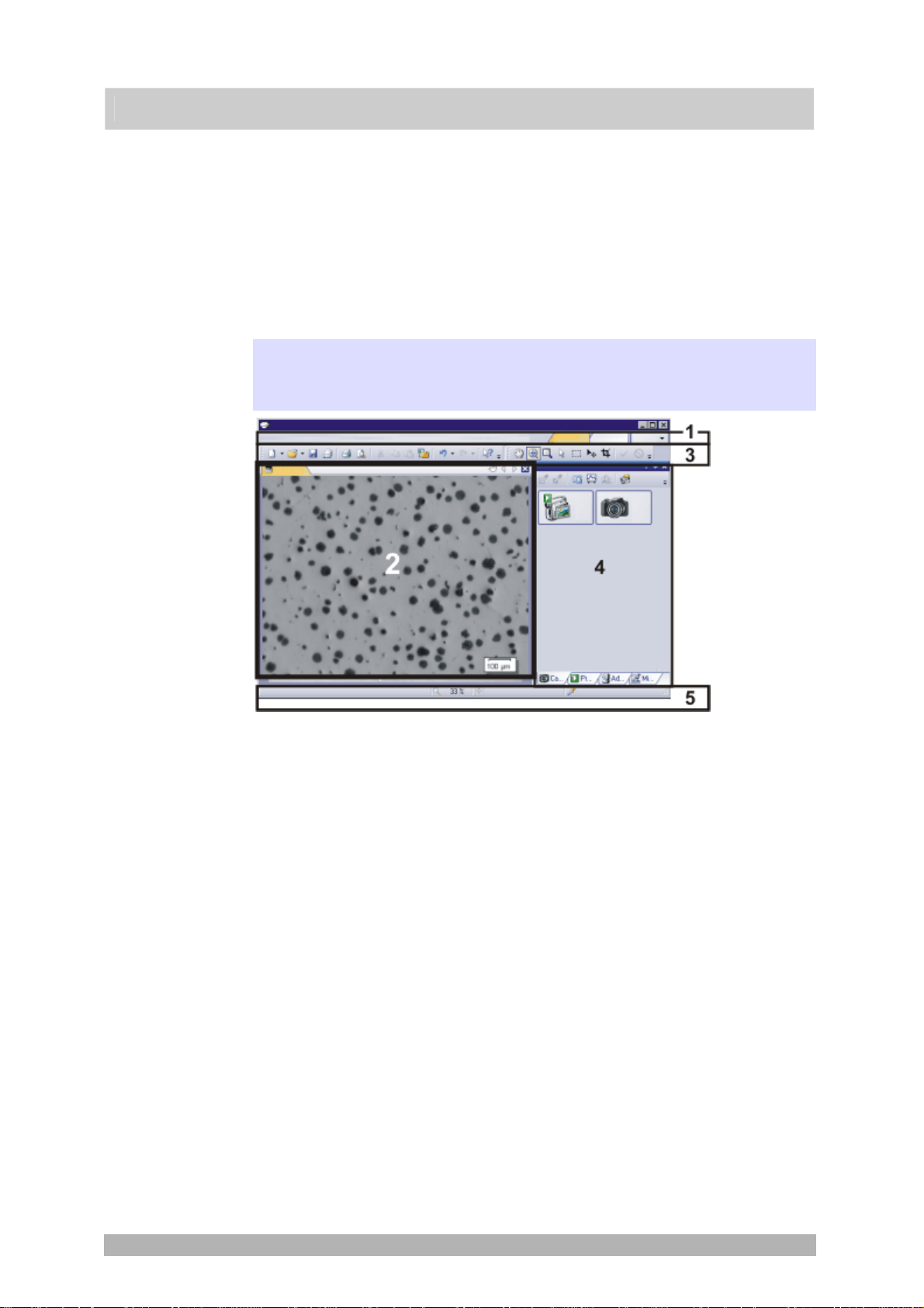
Appearance of the user

interface

User interface

(1) Men

(2) Docu

ment group

(3) T

(4) Tool windows

u bar

oolbars

The illustration shows the schematic user interface with its basic elements. You can call up many commands by using the corresponding menu. Your

software's menu bar can be configured to suit your requirements. Use the Tools

> Customization > Start Customize Mode... command to add menus, modify, or

delete them. Furthe

r information is available in the online help.

The document group contains all loaded documents. These can be of all supported document types. When you start your software, the document group is empty. While you use your software it gets filled - e.g., when you load or acquire images, or perform various image processing operations to change the source image and create a new one.

Comm

ands you use frequently are linked to a button providing you with quick and easy access to these functions. Please note, that there are many functions which are only accessible via a toolbar, e.g., the drawing functions required for annotating an image. Use the Tools > Customization > Start Customize Mode... command to modify a toolbar's appearance to suit your requirements.

Tool win functions. For example, in the Properties tool window you will find all the information available on the active document.

In contrast to dialog b long as they are switched on. That gives you access to the settings in the tool windows at any time.

dows combine functions into groups. These may be very different

oxes, tool windows remain visible on the user interface as

Page 6

(5) Status bar

The status bar shows a lot of information, e.g., a brief description of each function. Simply move the mouse pointer over the command or button for this information.

2.2. Overview - Layouts

To switch backwards and forwards between different layouts, click on the righthand side in the menu bar on the name of the layout you want, or use the View >

Layout command.

Which predefined

layouts are there?

hat is a layout?

hich elements of the

user interface belong to

the layout?

For important tasks several layouts have already been defined. The following layouts are available:

Acqui

re images ("Acquisition" layout) View and process images ("Processing" layout) Measuring images ("Count and Measure" layout) Generate a report ("Reporting" layout )

In contrast to your own layouts, predefined layouts can't be deleted. Therefore, you can always restore a predefined layout back to its originally defined form. To do this, select the predefined layout, and use the View > Layout > Reset Current

Layout command.

Your software's user interface is to a great extent configurable, so that it can easily be adapted to meet the requirements of individual users or of different tasks. You can define a so-called "layout" that is suitable for the task on hand. A "layout" is an arrangement of the control elements on your monitor that is optimal for the task on hand. In any layout, only the software functions that are important in respect to this layout will be available.

Example: The Camera Control tool window is only of importance when you acquire images. When instead of that, you want to measure images, you don't need that tool window. That's why the "Acquisition" layout contains the Camera Control tool window, while in the "Count and Measure" layout it's hidden.

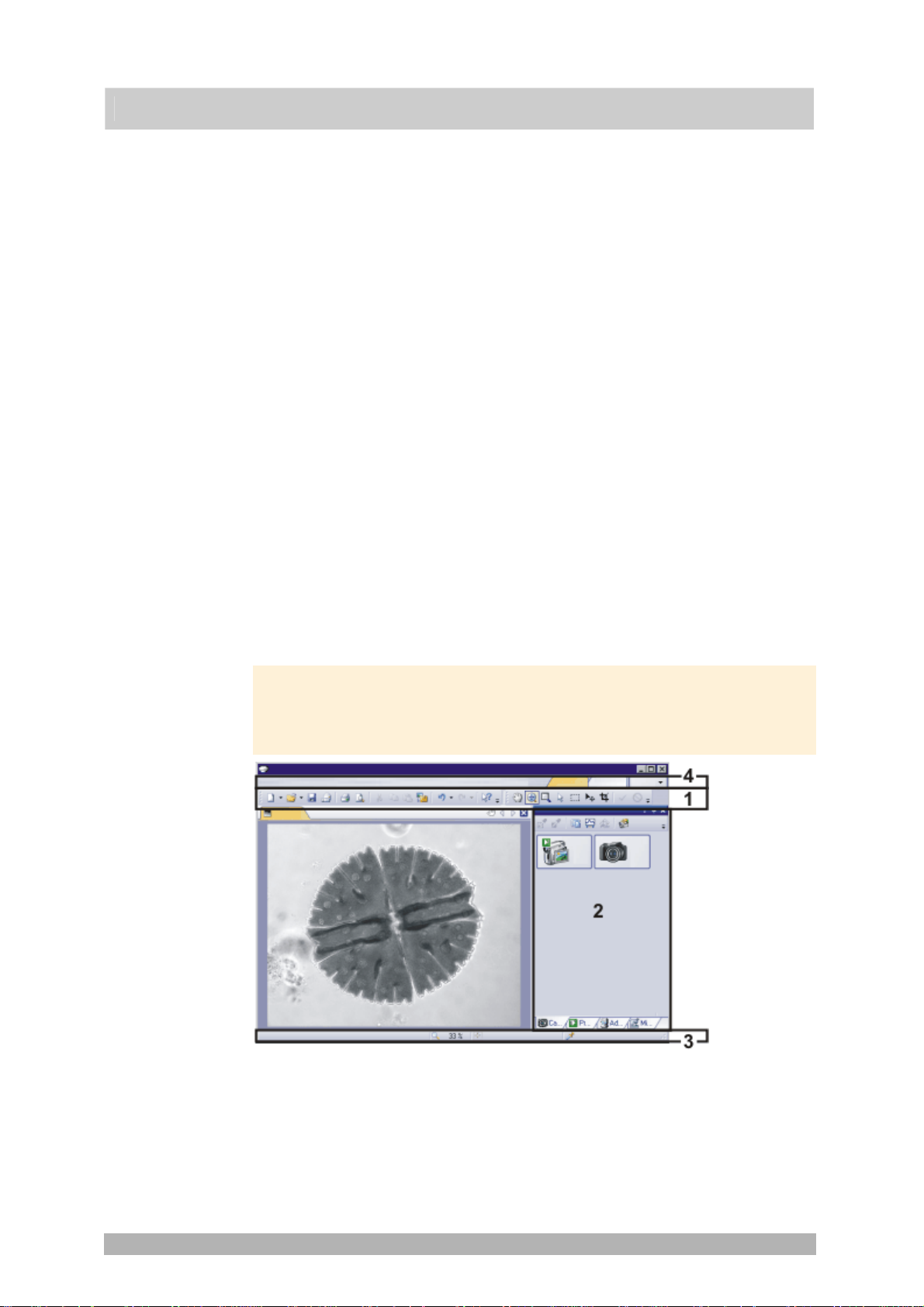
User interface

00108

The illustration shows you the elements of the user interface that belong to the layout. (1) Toolbars (2) Tool windows (3) Status bar (4) Menu bar

00013

Page 7

2.3. Document group

The document group contains all loaded documents. These can be of all supported document types.

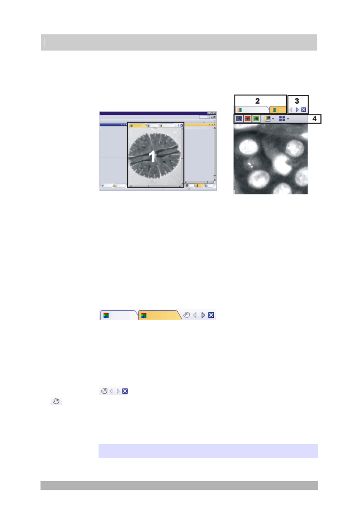
The illustration shows left, a schematic representation of a user interface. On the right, the document group is shown enlarged.

User interface

Button with a

hand

Document group in the user interface

You will find the document group in the middle of the user interface. In it you will find all of the documents that have been loaded, and naturally, all of the images that have been acquired also. Also the live-image and the images resulting from, e.g., any image processing function, will be displayed there.

Document bar in the document group

The document bar is the document group's header.

For every loaded document, an individual field will be set up in the document group. Click the name of a document in the document bar to have this document displayed in the document group. The name of the active document will be shown in color. Each type of document is identified by its own icon.

Buttons in the document bar

At the top right of the document bar you will see several buttons.

Click the button with a hand on it to extract the document group from the user interface. In this way you will create a document window that you can freely position or change in size.

If you would like to merge two do one of the two document groups. With the left mouse button depressed, drag the document group with all the files loaded in it, onto an existing one.

You can only position document groups as you wish when you are in the expert mode. In standard mode the button with the hand is not available.

cument groups, click the button with the hand in

Page 8

Arrow button

Button with a cross

The arrow buttons located at the top right of the document group are, to begin with, inactive when you start your software. The arrow buttons will only become active when you have loaded so many documents that all of their names can no longer be displayed in the document group. Then you can click one of the two arrows to make the fields with the document names scroll to the left or the right. That will enable you to see the documents that were previously not shown.

Click the butt saved, the Unsaved Documents dialog box will open. You can then decide whether or not you still need the data.

Navigation bar in the image window

Multi-dimensional images have their own navigation bar directly in the image window. Use this navigation bar to determine how a multi-dimensional image is to be displayed on your monitor, or to change this.

2.4. Tool Windows

Tool windows combine functions into groups. These may be very different functions. For example, in the Properties tool window you will find all the information available on the active document.

Which tool windows are shown by default depends on the layout you have chosen. You can, naturally, at any time, make specific tool windows appear and disappear manually. To do so, use the View > Tool Windows command.

Manually displayed or hidden tool windows will be saved together with the layout and are available again the next time you start the program. Resetting the layout using the View > Layout > Reset Current Layout command will have the result that only the tool windows that are defined by default will be displayed.

User interface

on with a cross to close the active document. If it has not yet been

00139

Docked tool windows

Freely positioned tool

windows

Position of the tool windows

The user interface is to a large degree configurable. For this reason, tool windows can be docked, freely positioned, or integrated in document groups.

Tool windows can be docked to the left or right of the document window, or below it. To save space, several tool windows may lie on top of each other. They are then arranged as tabs. In this case, activate the required tool window by clicking the title of the corresponding tab below the window.

You can only position tool windows as you wish when you are in the expert mode.

You can at a the way a dialog box does. To release a tool window from its docked position, click on its header with your left mouse button. Then, while keeping the left mouse button depressed, drag the tool window to wherever you want it.

ny time float a tool window. The tool window then behaves exactly

Page 9

Integrating a tool

window into a

document group

User interface

You can only add tool windows to a document group when you are in the expert mode.

You can integrate certain tool windows in the document group, for example, the

File Explorer tool window. To do this, use the Document Mode command. To

open a context menu containing this command, rightclick any tool window's header. The tool window will then act similarly to a document window, e.g., like an image window.

Use the Tool Wind document group. To open a context menu containing this command, rightclick any tool window's header.

ow Mode command, to float a tool window back out of the

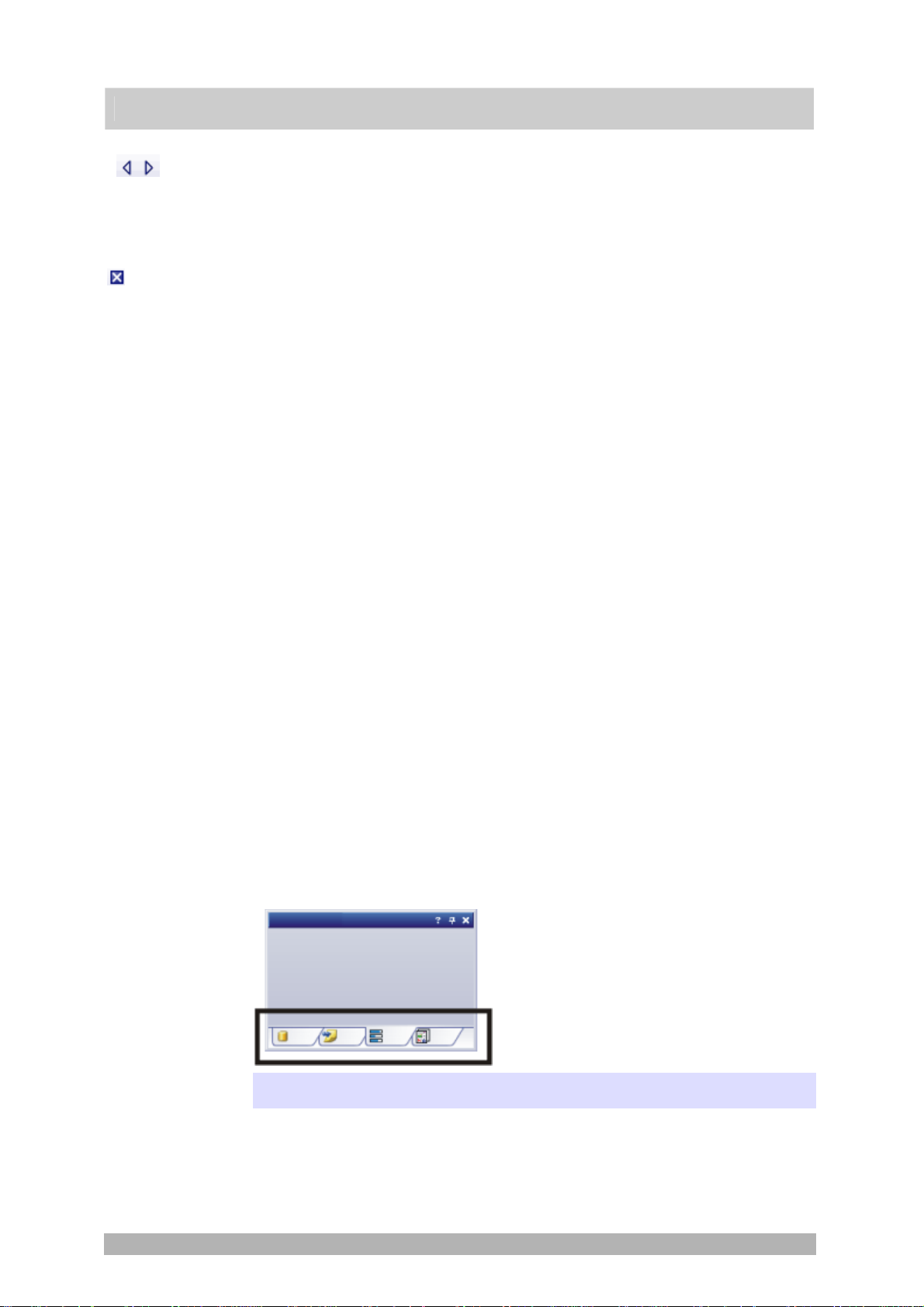
Buttons in the header

In the header of every tool window, you will find the three buttons Help, Auto

Hide and Close.

Click the Help button to open the online help for the tool window. Click the Auto Hide button to minimize the tool window. Click the Close button to hide the tool window. You can make it reappear at any time, for example, with the View > Tool Windows command.

Context menu of the header

To open a context menu, rightclick a tool window's header. The context menu can contain the Auto Hide, Document Mode, and Transparency commands. Which commands will be shown, depends on the tool window.

Additionally, the context menu contains a list of all of the tool windows that are available. Every tool window is identified by its own icon. The icons of the currently displayed tool windows appear clicked. You can recognize this status by the icon's background color. Use this list to make tool windows appear.

2.5. Working with documents

You can choose from a number of possibilities when you want to open, save, or close documents. As a rule, these documents will be images. However, your software supports several more document types. You will find a list of supported documents in the online help.

Saving documents

You should always save important documents immediately following their acquisition. You can recognize documents that have not been saved by the star icon after the document's name.

There are a number of ways in which you can save documents.

1. To save a single document, activate the document in the document group

and use the File > Save As... command.

2. Use the Documents tool window.

Select the desired document and use the Save command in the context menu. For the selection of documents, the standard MS-Windows conventions for Multiple Selection are valid.

00037

Page 10

Autosave and close

User interface

3. Use the Gallery tool window.

Select the desired document and use the Save command in the context menu. For the selection of documents, the standard MS-Windows conventions for Multiple Selection are valid.

4. Save your documents in a database That enables you to store all manner of

data that belongs together in one location. Search and filter functions make it quick and easy to locate saved documents. Detailed information on inserting documents into a database can be found in the online help.

1. When you exit your software, all of the data that has not yet been saved will

be listed in the Unsaved Documents dialog box. This gives you the chance to decide which document you still want to save.

2. With some acquisition processes the images will be automatically saved

when the acquisition has been completed. You will find an overview of the acquisition processes that are supported in the online help.

3. You can also configure your software in such a way that all images are saved

automatically after image acquisition. To do so, use the Acquisition Settings

> Saving dialog box.

There, you can also set that your images are automatically saved in a database, after image acquisition.

imm

ments

ediately

Closing all docu

Closing a document

Closing documents

There are a number of ways in which you can close documents.

1. Use the Documents tool window.

Select the desired document and use the Close command in the context menu. For the selection of documents, the standard MS-Windows conventions for Multiple Selection are valid.

2. To close a single document, activate the document in the document group

and use the File > Close command. Alternatively, you can click the button with the cross

. You will find this button on the top right in the document

group.

3. Use the Gallery tool window.

Select the desired document and use the Close command in the context menu. For the selection of documents, the standard MS-Windows conventions for Multiple Selection are valid.

To close all loaded documents use the Close All command. You will find this command in the File menu, and in both the Documents and the Gallery tool window's context menu.

To close a document immediately without a query, close it with the [Shift] key depresse

d. Data you have not saved will be lost.

Opening documents

There are a number of ways in which you can open or load documents.

1. Use the File > Open... command.

2. Use the File Explorer tool window.

To load a single image, doubleclick on the image file in the File Explorer tool window. To load several images simultaneously, select the images and with the left mouse button depressed, drag them into the document group. For the selection of images, the standard MS-Windows conventions for Multiple Selection are valid.

Page 11

Generating a test

Using sam

image

ple images

User interface

3. Drag the document you want, directly out of the MS-Windows Explorer, onto

your software's document group.

4. Use the Database > Load Documents command to load documents from the

database into your software. Further information is available in the online help.

If you want to get used to your software, then sometimes any image suffices to try out a function. Press [Ctrl + Shift + Alt + T] to generate a color test image. With the [Ctrl + Alt + T] shortcut, you can generate a test image that is made up of 256 gray values.

ng the installation of your software some sample images have been installed,

Duri too. You can find a sample image for each image type. Regarding the information as to where the example images are located, please refer to the online help. These example images might be of help to you when you familiarize yourself with your software.

Activating documents in the document group

There are several ways to activate one of the documents that has been loaded into the document group and thus display it on your monitor.

1. Use the Documents tool window. Click the desired document there.

2. Use the Gallery tool window. Click the desired document there.

3. Click the title of the desired document in the document group.

4. To open a list with all currently loaded documents, use the [Ctrl + Tab]

shortcut. Leftclick the document that you want to have displayed on your monitor.

5. Use the keyboard shortcut [Ctrl + F6] or [Ctrl + Shift + F6], to have the next

document in the document group displayed. With this keyboard shortcut you can display all of the loaded documents one after the other.

6. In the Window menu you will find a list of all of the documents that have been

loaded. Select the document you want from this list.

00143

Page 12

3. Configuring the system

Configuring the system

Why do you have to

configure the system?

hen do you have to

configure the system?

Switching off your

operating system's

hibernation m

ode

After successfully installing your software you will need to first configure your image analysis system, then calibrate it. Only when you have done this will you have made the preparations that are necessary to ensure that you will be able to acquire high quality images that are correctly calibrated. When you work with a motorized microscope, you will also need to configure the existing hardware, to enable the program to control the motorized parts of your microsco pe.

You will only need to comp

letely configure and calibrate your system anew when you have installed the software on your PC for the first time, and then start it. When you later change the way your microscope is equipped, you will only need to change the configuration of certain hardware components, and possibly also recalibrate them.

Whe

n you use the MS-Windows Vista operating system: Switch the hibernation mode off. To do so, click the Start button located at the bottom left of the operating system's task bar. Use the Control Panel command. Open the System and Maintenance > Power Options > Change when the

computer sleeps window. Here, you can switch off your PC's hibernation mode.

Process flow of the configuration

To set up your software, the following steps will be necessary:

Select the camera and the microscope

Select the cam

Specifying which

hardware is available

era and

the microscope

Configuring the

interfaces

Specifying which hardware is available

Configuring the interfaces

Configuring the specified hardware

Calibrating the system

The first time you start your software after the installation has been made, a quick configuration with some default settings will be made. In this step you need only to specify the camera and microscope types, in the Quick Device Setup dialog box. The microscope will be configured with a selection of typical hardware components. Further information is available in the online help.

Your software has to kno

w which hardware components your microscope is equipped with. Only these hardware components can be configured and subsequently controlled by the software. In the Acquire > Devices > Device List dialog box, you select the hardware components that are available on your microscope.

Use the Interf

aces dialog box, to configure the interface between your

microscope or other motorized components, and the PC on which your software runs.

Page 13

Configuring the

specified hardware

ating the system

Calibr

Configuring the system

Usually various different devices, such as a camera, a microscope and/or a stage, will belong to your system. Use the Acquire > Devices > Device S e ttings... dialog box to configure the connected devices so that they can be correctly controlled by your software.

Whe

n all of the hardware components have been registered with your software and have been configured, the functioning of the system is already ensured. However, it's only really easy to work with the system and to acquire top quality images, when you have calibrated your software. The detailed information that helps you to make optimal acquisitions, will then be available. Your software offers a wizard that will help you while you go through the individual calibration processes. Use the Acquire > Calibrations... command to start the software wizard.

00159

Page 14

4. Acquiring single images

You can use your software to acquire high resolution images in a very short period of time. For your first acquisition you should carry out these instructions step for step. Then, when you later make other acquisitions, you will notice that for similar types of sample many of the settings you made for the first acquisition can be adopted without change.

Acquiring a single image

1. Switch to the "Acquisition" layout. To do this, use, e.g., the View > Layout >

Acquisition command.

Acquiring single images

Selecting the objective

Switching on the live-

Setting the image

Acquiring and saving

quality

an im

age

2. In the Camera Control tool window, click the Live

button.

3. On the Microscope Control toolbar, click the button with the objective that

you use for the image acquisition. Go to the required specimen position in the live-image.

5. Bring the sample into focus. The Focus Indicator toolbar is there for you to

use when you are focusing on your sample.

Check the color reproduction. If necessary, carry out a white balance.

7. Check the exposure time. You can either use the automatic exposure time

function, or enter the exposure time manually.

8. Select the resolution you want.

9. On the Camera Control tool window, click the Snap



The image you have acquired will be shown in the document group.

button.

10. Use the File > Save As... command to save the image. Use the

recommended TIF file format.

00048

Page 15

Behavior of the live window

The behavior of the live window depends on the acquisition settings in the

Acquisition Settings > Acquisition > General dialog box.

Prerequisite

For the following step-by-step instructions, the Keep document when live is

stopped option is selected, and the Create new document when live is started

check box is cleared.

Switching the live-image on and off without acquiring an image

1. Make the Camera Control tool window appear. To do this, use, e.g., the View

> Tool Windows > Camera Control command.

Acquiring single images

2. Click the Live

 A temporary live window named "Live (a ctive)" is created in the

document group.

 The live-image will be shown in the live window.  You can always recognize the live modus by the changed look of the

Live

3. Click the Live

 The live mode will be switched off.  The active live-image will be stopped.  The live window's header will change to "Live (stopped)". You can save

the stopped live-image located in the live window just as you can every other image.

The live window may look similar to an image window, but it will be handled differently. The next time you switch on the live mode, the image will be overwritten. Additionally, it will be closed without a warning message when your software is closed.

button in the Camera Control tool window.

button again.

Switching to the live-image and acquiring an image

1. Make the Camera Control tool window appear. To do this, use, e.g., the View

> Tool Windows > Camera Control command.

2. Click the Live

 A temporary live window named "Live (active)" will be created in the

document group.

 The live-image will be shown in the live window.  You can always recognize the live modus by the changed look of the

Live

3. Click the Snap

button in the Camera Control tool window.

button.

Page 16

Acquiring single images

 The live mode will be switched off. The live window's header will change

to "Live (stopped)".

 At the same time, a new image document will be created and displayed

in the document group. You can rename and save this image. If you have not already saved it when you end your software, you will be asked if you want to do so.

Displaying the live-image and the acquired images simultaneously

Task

You want to view the live-image and the acquired images simultaneously. When you do this, it should also be possible to look through the acquired images without having to end the live mode.

Close all open documents.

2. Open the Acquisition Settings > Acquisition > General dialog box.

To do so, click, e.g., the Acquisition Settings

Control tool window.

3. There, make the following settings:

 Choose the Keep document when live is stopped option.  Clear the Create new document when live is started check box.  Select the Continue live after acquisition check box.

4. Switch to the live mode. Acquire an image, then switch the live mode off

again  Both of the image windows "Live (sto pped)" and "Image_<Serial No.>"

are now in the document group.

 The "Live (stopped)" image window is active. That's to say, right now you

see the stopped live-image in the document group. In the document bar, the Name "Live (stopped)" is highlighted in color.

5. Split the document group, to have two images displayed next to each other.

That's only possible when at least two images have been loaded. That's why you created two images in the first step.

6. Use the Window > Split/Unsplit > Split/Unsplit Document Group (Left).

 This comman d creates a new document group to the left of the current

document group. In the newly set up document group, the active document will be automatically displayed. Since in this case, the active document is the stopped live-image, you will now see the live window on the left and the acquired image on the right.

7. Start the live mode.

 In the document group, the left window will become the live window Live

(active)". Here you see the live-image.

8. Activate the document group on the right. To do so, click, for example, the

image displayed there.

button on the Camera

9. Click the Snap

 The acquired image will b e displayed in the active document group. In

this case, it's the document group on the right.

 After the image acquisition has be en made, the live-image will

automatically start once more, so that you'll then see the live-image again on the left.

button.

Page 17

Acquiring single images

 While the live-image is being shown on the left, you can switch as often

as you want between the images that have up till then been acquired.

You can set up your software's user interface in such a way that you can view the live-image (1) and the images that have up till then been acquired (2), next to one another.

00181 25072011

Page 18

5. Acquiring image series

5.1. Time stack

What is a time stack?

You can combine a series of separate images into one image. In a time stack all frames have been acquired at different points of time. A time stack shows you how an area of a sample changes with time. You can play back a time stack just as you do a movie.

A standard image is two dimensional. The position of every pixel will be determined by its X- and Y-values. With a time stack, the time when the image was acquired is an additional piece of information or "dimension" for each frame.

The frames making up a time stack can be 8-bit gray-value images, 16-bit grayvalue images, or 24-bit true-color images.

Note: A time stack can also be an AVI video. You can load and play back the AVI file format with your software.

Acquiring image series

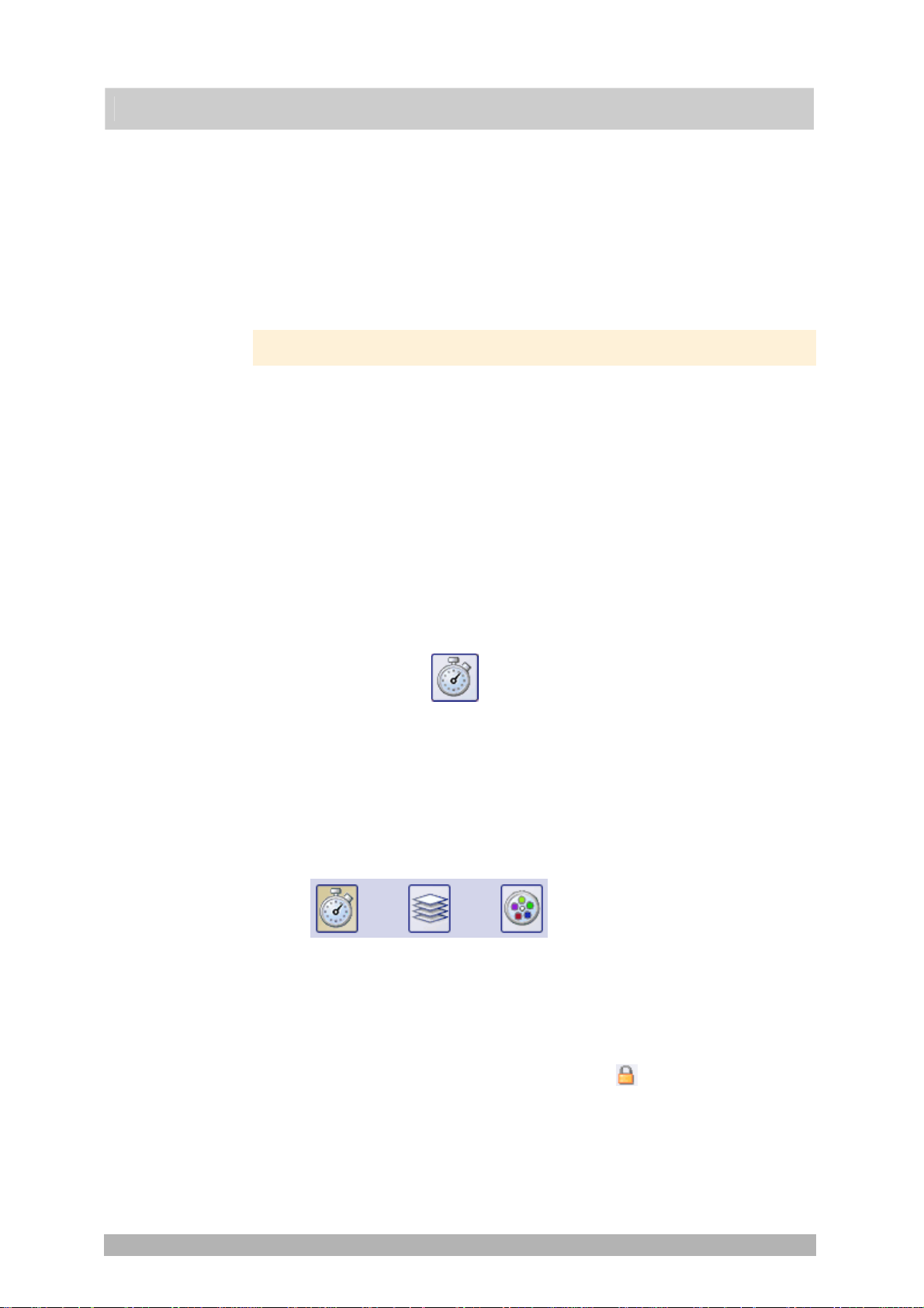
How do I recognize a time stack?

You can immediately recognize the different image types by the icon which appears in front of the image name in the document group, or in the Documents tool window. When it is a time stack, this icon will be supplemented by a small

clock. A time stack that is made up of true-color images has, e.g., this icon In the Properties tool window, you can use the Frame Count entry to find out how

many individual images are contained in any given image. A time stack will automatically have its own navigation bar directly in the image

window. Use this navigation bar to browse through the frames making up a time stack, or to play back the time stack like a movie. Further information on the navigation bar is available in the online help.

Creating time stacks

There are different ways in which you can generate a time stack. To acquire a time stack, use one of the two acquisition processes Time Lapse or

Movie.

Use the Image > Combine Frames… command, to have several individual images combined into a time stack. A detailed description of the Combine

Frames dialog box can be found in the online help. .

Displaying time stacks

A time stack contains much more data than can be displayed on your monitor. A time stack will automatically have its own navigation bar directly in the image

window. Use this navigation bar to determine which of the frames from a time

Page 19

Hiding the navigation

Acquiring image series

stack is to be displayed on your monitor. You can also play back a time stack just as you would a movie.

Alternatively, you can also use the Dimension Selector tool window, to determine how a time stack is to be displayed on your monitor, or to change the display.

You can also hide the navigation bar. To do this, use the Tools > Options...

bar

command. Select the Images > General entry in the tree view. Clear the Show

image navigation toolbar check box.

Saving time stacks

When you save time stacks, you will, as a rule, use the VSI file format. Only when you use this file format is there no limit to the size a time stack can be. When you save smaller time stacks, you can also use the TIF or the AVI file format. With any other file format you will lose most of the image information during saving. Use the File > Save As... command.

Converting time stacks

Breaking down time

stacks into individual

images

Reducing the number

of frames within a time

stack

Converting time stacks

while saving them

Use the Image > Separate > Time Frames menu command, to have a time stack broken down into selected individual images.

It is possible that, within a time stack, only a short period of time interests you. Use the Extract command, to create a new time stack that only contains a selection of frames, from an existing time stack. In this way, you will reduce the number of frames within a time stack to only those that interest you. You will find this command in the context menu in the tile view for time stacks. Further information on this command is available in the online help.

When you save a time stack in another file format as TIF or VSI, the time stack will also be converted. The time stack will then be turned into a standard truecolor image. This image shows the frame that is at that moment displayed on the monitor.

Processing time stacks

Image processing operations, e.g., a sharpen filter, affect either the whole image or only a selection of individual images. You can find most of the image processing operations in the Process menu. The dialog box that is opened when you use an image processing operation is made up in the same way for every operation. In this dialog box, select the Apply

on > Selected frames and channels option, to determine that the function only

affects the selected frames. Select the Apply on > All frames and channels option, to process all of the

individual images. Select the individual images that you want to process, in the tile view. Further

information on mthis image window view can be found in the online help. Look through the thumbnails and select the images you want to process. In the tile view, the standard MS-Windows conventions for multiple selection are valid.

An image processing operation does not change the source image's dimensions. The resulting image is, therefore, comprised of the same number of separate images as the source image.

00011

Page 20

5.2. Time Lapse / Movie

Acquiring image series

When is it better for me

to acquire a time stack?

Saving a time stack as

an AVI

When is it better for me

to acquire a movie?

Both the Time Lapse and the Mov sample changes with time. What i

ie acquisition processes document the way a

s the difference between the two processes?

Use the "Time Lapse" acquisition process in the following cases:

 Use the "Time Lapse" acq uisition process when processe

s that run slowly are to be documented, e.g., where an acquisition is to be made only every 15 minutes.

 Use the "Time Lapse" acquisition process when, while the acquisition is

in progress, you want to see the frames that have already been acquired, for example, to check on how an experiment is progressing. To do this,

click the Tile View

button in the navigation bar in the image window.

 Use the "Time Lapse" acq uisition process when you want to use those of

your software's add al functions that can only be saved in the VSI or ition TIF file format. For example, to measure objects, to insert drawing elements such a s arrows, or a text

, or to have the acquisition parameters for the camera

and microscope that you've used, available at any time in the future.

 Use the "Time Lapse" acq uisition process when the important thing is to

achieve an optimal image quality, and the size of the file is no problem

You can al

so save a time stack as an AVI file, at a later date. To do this, load the time stack into the document group, select the File > Save as... command, and select the AVI file type. Make, if necessary, additional settings in the Select AVI

Save Options dialog box.

Use the "Movie" acquisition process in the following cases:

 Use the "Movie" acquisition process when processe

s that run very quickly are to be documented (the number of acquisitions per second is considerably higher with movies than with time stacks).

 Use the "Movie" acquisition process when you want to give the movie to

third persons who do not have this software (AVI files can also be played back with the MS Media Player).

 Use the "Movie" acquisition process when keeping file sizes small is of

great importance.

0010

Page 21

5.3. Acquiring movies and time stacks

With your software you can acquire movies and time stacks.

Acquiring a movie

You can use your software to record a movie. When you do this, your camera will acquire as many images as it can within an arbitrary period of time. The movie will be saved as a file in the AVI format. You can use your software to play it back.

1. Switch to the "Acquisition" layout. To do this, use, e.g., the View > Layout >

Acquisition command.

Selecting the objective

Selecting the storage

com

pression method

Setting the im

location

Selecting the

quality

2. On the Microscope Control toolbar, click the button with the objective that you want to use for the movie acquisition.

3. In

the Camera Control tool window's toolbar, click the Acquisition Settings

button.

 The Acq

uisition Settings dialog box will open.

4. Select the Saving > Movie entry in the tree structure.

5. Decide how you want to save the recorded movies after the acquisition process is finished. Select the Filesystem entry in the Automatic save >

Destination list to automatically save the movies you have acquired.

 The Base field located in the Directory group shows the directory that will

currently be used when your movies are automatically saved.

6. Click the [...] button next to the Base field to alter the directory. 

The AVI file format is preset in the File type list. This is a fixed setting that cannot be changed.

7. Click the Options... button if you want to compress the AVI file in order to reduce the movie's file size.

8. From the Compression list, select the M-JPEG entry and confirm with OK.

Please note: Compressing the movie is only possible if the selected compression method (codec) has already been installed on your PC. If the compression method has not been installed the AVI file will be saved uncompressed. The selected compression method must also be available on the PC that is used for playing back the AVI. Otherwise the quality of the AVI may be considerably worse when the AVI is played back.

9. Close the Acquisition Settings dialog box with OK.

age

10. Switch to the live mode, and select the optimal settings for movie recording, in the Camera Control tool window. Pay special attention to setting the correct exposure time.



This exposure time will not be changed during the movie recording.

11. Find the segment of the sample that interests you and focus on it.

Acquiring image series

Page 22

Switching to the "Movie

recording" mode

Acquiring image series

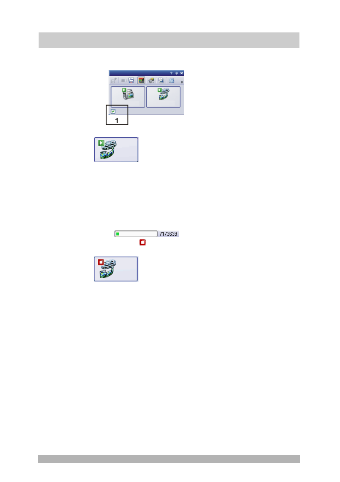
12. Select the Movie recording check box (1). The check box can be found below the Live button in the Camera Control tool window.

Starting m

Stopping movie

ovie

recording

rec

ording

 The Snap button will be replaced by the Movie button.

13. Click the Movie button to start the movie recording.  The live-image will be shown and the recording of the movie will start

immediately.

 In the status bar a prog ress indicator is displayed. At the left of the slash

the number of already acquired images will be indicated. At the right of the slash an estimation of the maximum possible number of images will be shown. This number depends on your camera's image size a nd cannot exceed 2GB.

 This icon

on the Movie button will indicate that a movie is being

recorded at the moment.

14. Click the Movie button again to end the movie recording.

 The first image of the movie will be displayed.  The navigation bar for time stacks will be shown in the document group.

Use this navigation bar to play the movie.

 The software will remain in the "Movie recording" mode until you clear

the Movie recording check box once more.

Page 23

Selecting the objective

Setting the im

quality

Selecting the

acquisition process

Task

age

Acquiring image series

Acquiring a time stack

In a time stack all frames have been acquired at different points of time. With a time stack you can document the way the position on the sample changes with time. To begin with, for the acquisition of a time stack make the same settings in the Camera Control tool window as you do for the acquisition of a snapshot. Additionally, in the Process Manager tool window, you have to define the time sequence in which the images are to be acquired.

You want to acquire a time stack over a period of 10 seconds. One image is to be acquired every second.

Switch to the "Acquisition" layout. To do this, use, e.g., the View > Layout >

Acquisition command.

2. On the Microscope Control toolbar, click the button with the objective that you want to use for the image acquisition.

Switch to the live mode, and select the optimal settings for your acquisition, in the Camera Control tool window. Pay special attention to setting the correct exposure time. This exposure time will be used for all of the frames in the time stack.

Choose the resolution you want for the time stack's frames, from the

Resolution > Snap/Process list.

5. Find the segment of the sample that interests you and focus on it.

6. Activate the Process Manager tool window.

7. Select the Automatic Processes option.

acquisition param

Selecting the

eters

8. Click

the Time Lapse

button.

 The button will appear clicked. You can recognize this status by the

button's colored background.

 The [ t ] group will be automatically displayed in the tool window.

9. Should another acquisition process be active, e.g., Multicolor, click the button to switch off the acquisition process.

 The group with the various acq uisition processes should now look like

this:

10. Clear the check boxes Delay and As fast as possible.

11. Specify the time that the complete acquisition is to take, e.g., 10 seconds. Enter the value "00000:00:10" (for 10 seconds) in the Recording time field. You can directly edit every number in the field. To do so, simply click in front of the number you want to edit.

12.

Select the radio button on the right-hand side of the field to specify that the acquisition time is no longer to be changed. The

lock icon will

automatically appear beside the selected radio button.

13. Specify how many frames are to be acquired. Enter e.g., 10 in the Cycles field.

 The Interval field will be updated. It shows you the time that will elapse

between two consecutive frames.

Page 24

Acquiring a time stack

14. Click the Start button. 

The acquisition of the time stack will start immediately.

Acquiring image series

 The Start Process button changes into the Pause

this button will interrupt the acquisition process.

 The Stop

the acquisition process. The images of the time stack acquired until this moment will be preserved.

 At the bottom left, in the status bar, the progress bar will appear. It

informs you about the number of images that are still to be acquired.

 The acquisition has been completed when you can once more see the

Start

bar has been faded out.

 You will see the time stack you've acquired in the ima ge window. Use the

navigation bar located in the image window to view the time stack. Further information on the navigation bar is available in the online help.

 The time stack that has been acquired will be automatically saved. The

storage directory is shown in the Acquisition Settings > Saving > Process

Manager dialog box. The preset file format is VSI.

Note: When other programs are running on your PC, for instance a virus scanning program, it can interfere with the performance when a time stack is being acquired.

button will become active. A click on this button will stop

button in the Process Manager tool window, and the progress

button. A click on

00304 12012011

5.4. Z-stack

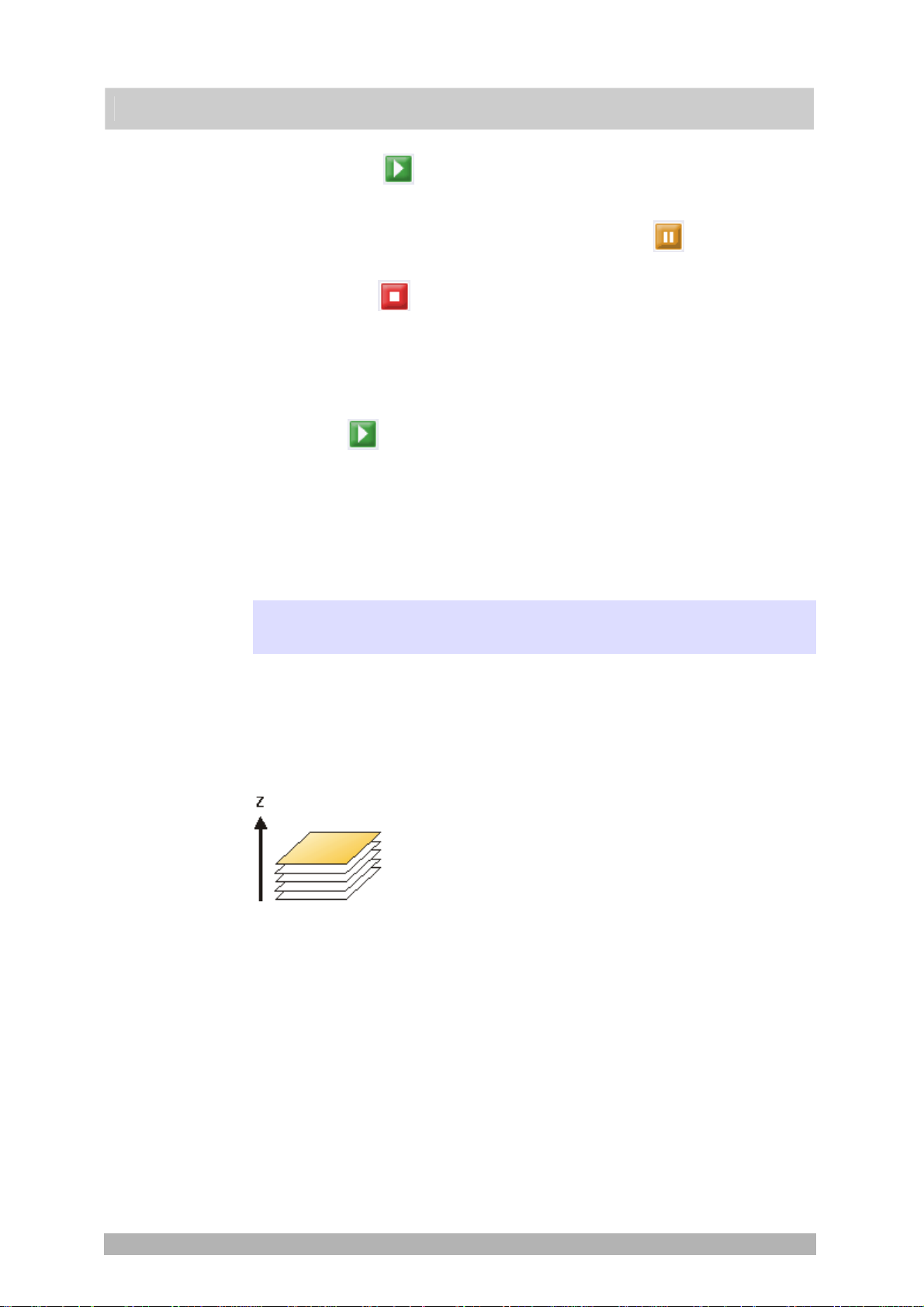
What is a Z-stack?

You can combine a series of separate images into one image file. A Z-stack contains frames acquired at different focus positions. A Z-stack is needed, e.g., for calculating an EFI image by the Process > Enhancement > EFI Processing... command.

A standard image is two dimensional. The position of every pixel will be determined by its X- and Y-values. With a Z-stack, the focus position or the height of the sample is an additional item of information for every pixel.

The frames making up a Z-stack can be 8-bit gray-value images, 16-bit-grayvalue images or 24-bit-true-color images.

Page 25

Acquiring image series

How do I recognize a Z-stack?

You can immediately recognize a multi-dimensional image by its icon which appears in front of the image name in the document group or in the Documents

tool window. When it is a Z-stack, this icon will be supplemented by a small Z

In the Properties tool window, you can use the Frame Count entry to find out how many individual images are contained in any given image.

A Z-stack image will automatically have its own navigation bar directly in the image window. Use this navigation bar to browse through the frames making up a Z-stack, or to play back the Z-stack like a movie. Further information on this navigation bar is available in the online help.

Creating a Z-stack

There are different ways in which you can generate a Z-stack.

1. To acquire a Z-stack, use the "Z-Stack" acquisition process.

2. Use the Image > Combine Frames… command, to have several

separate images combined into a Z-sta ck.

Breaking down Z-

stacks into separate

Reducing the nu

of frames within a Z-

Conver

while saving them

images

mber stack

ting Z-stacks

Displaying a Z-stack

A Z-stack contains much more data than can be displayed on your monitor. A Z-stack image will automatically have its own navigation bar directly in the

image window. Use this navigation bar to determine which of the frames from a Z-stack is to be displayed on your monitor. You can also play back the Z-stack just as you would a movie.

Alternatively, you can also use the Dimension Selector tool window, to set how a Z-stack is to be displayed on your monitor, or to change the display.

Saving a Z-stack

Please note: Z-stacks can only be saved in the TIF or VSI file format. Otherwise they loose a great deal of their image information during saving.

Converting a Z-stack

Use the Image > Separate > Height Frames menu command, to have a Z-stack broken down into selected frames.

It is possi

Extract command, to create a new Z-stack that only contains selected frames,

from an existing Z-stack. In this way, you will reduce the number of frames within a Z-stack to only those that interest you. You can find this command in the context menu in the tile view for Z-stacks.

Whe automatically be converted. The Z-stack will then be turned into a standard truecolor image. This image shows the frame that is at that moment displayed on the monitor.

ble that, within a Z-stack, only a short Z-range interests you. Use the

n you save a Z-stack in another file format as TIF or VSI, the Z-stack will

00012

Page 26

5.5. Acquiring a Z-stack

With the Z-Stack acquisition process, you acquire a series of frames one after the other, a Z-stack.

Acquiring a Z-stack

Example: You want to acquire a Z-stack. The sample is approximately 50 µm thick. The Z-distance between two frames is to be 2 µm.

1. Switch to the "Acquisition" layout. To do this, use, e.g., the View > Layout >

Acquisition command.

Selecting the objective

Setting the im

quality

Selecting the

acquisition process

2. On the Microscope Control toolbar, click the button with the objective that you want to use for the image acquisition.

age

Switch to the live mode, and select the optimal settings for your acquisition,

3. in the Camera Control tool window. Pay special attention to setting the correct exposure time. This exposure time will be used for all of the frames in the Z-stack.

Search out the required position in the sample.

5. Activate the Process Manager tool window.

6. Select the Automatic Processes option.

Acquiring image series

acquisition param

Selecting the

Acquiring an im

eters

age

7. Click

the Z-Stack

button.

 The button will appear clicked. You can recognize this status by the

button's colored background.

 The [ Z ] group will be automatically displayed in the tool window.

8. Should another acquisition process be active, e.g., Multi Channel, click the button to switch off the acquisition process.

 The group with the various acq uisition processes should now look like

this:

9. Select the Range entry in the Define list.

10. Enter the Z-range you want, in the Range field. In this example, enter a little more than the sample's thickness (= 50 µm), e.g., the value 60.

the Step Size field, enter the required Z-distance, e.g., the value 2, for a Z-

11. In distance of 2 µm. The value should correspond with your objective's depth of focus.

 In the Z-Slices field you will then be shown how many frames are to be

acquired. In this example, 31 frames will be acquired.

12. Find the segment of the sample that interests you and focus on it. To do this, use the arrow buttons in the [ Z ] group. The buttons with a double arrow move the stage in larger steps.

13. Click the Start

button.

Page 27

Acquiring image series

 Your software now moves the Z-drive of the micro scope sta ge to the

start position. The starting positions lies half of the Z-range deeper than the stage's current Z-position.

 The acquisition of the Z-st ack will begin as soon as the starting position

has been reached. The microscope stage moves upwards step by step and acquires an image at each new Z-position.

 You can see the acquired Z-stack in the image window. Use the

navigation bar located in the image window to view the Z-stack. Further information on the navigation bar is available in the online help.

00367

Page 28

Acquiring fluorescence images

6. Acquiring fluorescence images

6.1. Multi-channel image

What is a multi-channel image?

A multi-channel image combines a series of monochrome images into one image. The multi-channel image usually shows a sample that has been stained with several different fluorochromes. The multi-channel image is made up of a combination of the individual fluorescence images. You can have the individual fluorescence images displayed separately or also as a superimposition of all of the fluorescence images.

The separate images'

times stack or Z-stack

image type

Combination with

At the top of the illustration you can see the individual fluorescence images (1). Below, you can see the superimposition (2) of the separate fluorescence images.

The separate images making up a multi-channel image can be 8-bit gray-value images, or 16-bit gray-value images.

A multi-cha channel time stack, for instance, then incorporates several color channels. Every color channel incorporated in the image is reproduced with its own time stack.

nnel image can be combined with a time stack or a Z-stack. A multi-

How do I recognize a multi-channel image?

You can immediately recognize a multi-channel image by this icon which appears in front of the image name in the document group or in the Documents tool window.

In the Properties tool window, you can use the Channels entry, to find out how many channels are contained in any given image.

A multi-channel image will automatically have its own navigation bar, directly in the image window. Use this navigation bar to set how a multi-channel image is to be displayed in the image window, or to change this.

Further information on the navigation bar for multi-channel images is available in the online help.

Page 29

Using the navigation

Acquiring fluorescence images

Creating multi-channel images

Your software offers you several ways of acquiring a multi-channel image. Use the Multi Channel automatic acquisition process to acquire a multi-channel

image. Use the Image > Combine Channels… command, to have several separate images combined into a multi-channel image.

Displaying multi-channel images

A multi-channel image contains much more data than can be displayed on your monitor.

bar

Hiding the navigation

Using the "Di Selector" tool window

bar

mension

When you load a multi-channel image into your software, you'll see a navigation bar in the image window, that provides you with access to all of the fluorescence channels.

 You can have the individual fluorescence images displayed separately or

also as a superimposition of all of the fluorescence images (1).

 Should you have acquired a brightfield o f the sample together with the

fluorescence images, you can make this brightfield appear or disappear (2).

 The individual fluorescence images are monochrome. For this reason,

you can change the color mapping however you like. You can display the fluorescence channels in the fluorescence colors, use a pseudo color

table of your choice, or also display the original images (3). Further information on the navigation bar for multi-channel images is available in the online help.

You can also hide the navigation bar. To do this, use the Tools > Options... command. Select the Images > General entry in the tree view. Clear the Show

image navigation toolbar check box.

Alternatively, you can al

so use the Dimension Selector tool window, to set how a multi-channel image is to be displayed on your monitor, or to change this. There you can, for example, change the fluorescence colors for individual color channels.

Saving multi-channel images

Please note: Multi-channel images can only be saved in the TIF or VSI file format. Otherwise they loose a great deal of their image information during saving.

Page 30

Acquiring fluorescence images

Converting multi-channel images

Breaking down a multi-

channel image into its

color channels

Reducing the color

channels in a m

channel image

Converting m

channel images while

saving them

ulti-

Use the Separate command, to have a multi-channel image broken down into chosen color channels. The resulting images are still of the "multi-channel" type, contain though, only one color channel.

There are

several ways of accessing this command:

 Click the Separate Channels button in the Dimension Selector tool

window.

 Use the Separate command from the Dimension Selector tool window's

context menu.

 Use the Image > Separate > Channels menu command. Use the Extract command, to create a new multi-channel image that is made up of fewer color channels than the source image.

Select all of the color channels you wish to retain, in the Dimension Selector tool window. Then use the Extract command in the tool window's context menu.

n you save a multi-channel image in another file format as TIF or VSI, the

Whe multi-channel image will also be converted. The multi-channel image then becomes a standard 24-bit true-color image. This image will always show exactly what is currently displayed on your monitor, that is to say, e.g., the superimposition of all of the channels or possibly only one channel.

Processing multi-channel images

Image processing operations, e.g., a sharpen filter, affect either the whole image or only a selection of individual images. You can find most of the image processing operations in the Process menu. Click here for more information on working with image processing operations.

Select the individual images that you want to process in the Dimension Selector tool window. The frames you have selected will be highlighted in color in the tool window.

The dialog box that is opened when you use an image processing operation is made up in the same way for every operation. In this dialog box, select the Apply

on > Selected frames and channels option, to determine that the function only

affects the selected frames. Select the Apply on > All frames and channels option, to process all of the

individual images. An image processing operation does not change the source image's dimensions.

The resulting image is, therefore, comprised of the same number of separate images as the source image.

00010

Page 31

Acquiring fluorescence images

6.2. Before and after you've acquired a fluorescence image

Before you acquire a fluorescence image

Defining observation

fluorescence image

methods

Setting up the

icroscope for the

acquisition of a

1. Define observation methods for your color channels.

2. Use

3. Click the required objective's button.

4. Click the button for the observation method with the excitation that has the

the View > Tool Windows > Microscope Control command, to make the

Microscope Control tool window appear.



In the Objectives group, you will find the buttons you use to change objectives.

 In the Observation method group, you can find a button for every

observation method that has been defined. Observation methods should have been defined at least for brightfield and for every color channel.

longest excitation wavelength (e.g., "Red")

Setting up the camera for the acquisition of a fluorescence image

5. Use the View > Tool Windows > Camera Control command to make the

Camera Control tool window appear.

6. Set the image resolution for the acquisition. With a high objective magnification, you require a lower resolution. For this purpose, select the required resolution from the Snap/Process list, located in the Resolution group.

7. Reduce the image resolution in the live mode. When you use a higher binning in the live mode, the frame rate will be reduced, which enables you to focus better. For this purpose, select an entry, e.g., with the supplement "(Binning 2x2)", from the Live/movie list, located in the Resolution group.

8. Should you work with a color camera: Switch on your camera's grayscale mode. The Toggle RGB/Grayscale mode button should now look like this

Switching off the

orrections for

brightfield acquisitions

Focusing a

fluorescence sam

ple

. You can find this button on the Camera Control tool window's toolbar.

9. If it's possible to set different bit depths with your camera, click the Toggle

Bitdepth

10. Use the View > Toolbars > Calibrations command, to have the Calibrations toolbar displayed.

11. Switch off the white balance and the shading correction. To do that, release these buttons

12.

Select the automatic exposure time.

button to set the maximum bit depth.

, if they are there and available.

Page 32

Acquiring fluorescence images

13. In the Camera Control tool window, click the Live button.  Should the live-image be too dark, select a higher value in the Camera

Control > Exposure > Exposure compensation list.

 Should the exposure time become longer than 300 ms, reduce it by

increasing the sensitivity or gain.

14. Bring the sample into focus.  In the camera's black & white mode, you can reduce the diffused light.

Setting the storage

Viewing a m

location

ulti-channel

image

Click the Online-Deblur

button, located in the Camera Control tool window's toolbar. You can then decide whether or not you want to apply the deconvolution filter. It's possible that you might have to lengthen the exposure time via the exposure time correction.

15. Finish the live mode. To do so, click the Live

button in the Camera

Control tool window, once more.

Multi-channel images will be saved by default, as soon as the acquisition has been completed. As file format, the VSI file format will be used.

16. Before you start the acquisition, specify where the file is to be saved.

17. To do this, click the Acquisition Settings

button, located in the Process

Manager tool window's toolbar. Select the Saving > Process Manager entry

in the tree view.  You can find the current directory in the Dire ct o ry > Base field.

18. Click the [...] button next to the Base field, to change the directory into which the image is to be saved after its acquisition.

After you've acquired a fluorescence image

A multi-channel image is made up of the individual fluorescence images. You can set which color channels, resp. combination of color channels, will be displayed on your monitor. To do this, use the navigation bar in the image window.

Click a color f channels that are at the moment displayed on your monitor will be identified by an eye icon.

The navigation bar also offers you additional possibilities for changing the appearance of the multi-channel image. Below, is an illustration of the navigation bar, click one of its buttons and you'll see a description of its functions.

ield to make the channel appear or disappear. All of the color

"Prope

Saving m

rties" tool

window

ulti-channel

images

Numerous acquisition parameters will be saved together with the image. Use the View > Tool Windows > Properties command, to make the Properties

tool window appear. In the Properties tool window, you can find that every color channel has its own Channel information group. This contains the channel name, the emission wavelength, the name of the observation method and the exposure time.

The multi-cha

nnel image will be automatically saved. You can set the storage directory in the Acquisition Settings > Saving > Process Manager dialog box. The file format used is VSI.

For the VSI format, a JPE

G compression of 90% is preset. You can change the

compression in the Acquisition Settings dialog box under Saving > Process

Manager > Automatic save > Options… .

Page 33

Acquiring fluorescence images

6.3. Defining observation methods for the fluorescence acquisition

Before you acquire a fluorescence image, you have to define observation methods for your color channels. As a rule, observation methods that you can adapt for your microscope configuration, have already been predefined.

Prerequisite

The system has already been configured and calibrated. For this purpose, you have to enter your hardware components in the Acquire > Devices > Device List dialog box, and configure them in the Device Settings dialog box. To finalize this action, calibrate your system by using the Acquire > Calibrations... command.

The table not motorized, microscopes. Only the hardware components that are relevant for the acquisition of multi-channel fluorescence images are listed.

s that follow, contain example configurations for both motorized, and

00363

Device List

Microscope Frame <Name of your

microscope>

Nosepiece <Name of your

nosepiece>

Mirror Turret <Name of your mirror

turret>

Stage Z-axis <Name of your

controller for the stage's Z-drive>

Fluorescence/reflected lightpath Shutter <Name of the

reflected light shutter>

Example entries

Non-motorized microscope

BX51 BX61

Manual Nosepiece Motorized (UCB)

Manual Mirror Turret

Not Motorized Motorized (UCB)

Manual Shutter Motorized (UCB)

Motorized microscope

BX-RFAA

Transmission lightpath Lamp <Name of your

transmission lamp>

Condenser <Name of your

condenser>

Not used UCB Halogen-Lamp

Manual Condenser U-UCD8A

Page 34

Device Settings Entries

Nosepiece <Your objectives> Mirror Turret U-MNU

U-MWB U-MWG For a position where there is no mirror cube, select the Free entry.

Condenser With a motorized condenser:

The hardware components Aperture Stop and Top Lens are additionally listed under the device settings.

Defining the observation method for transmission brightfield

Acquiring fluorescence images

Setting up the

mirror turret

For motorized

microscopes: Setting

up the condenser

Hardware components in transmission brightfield: In transmission brightfield, there is no fluorescence mirror cube in the light path. The reflected light shutter is closed.

1. Use the Acquire > Devices > Device Cust omization... command. Activate the

Observation Methods tab.

2. Click the New Observation Method

button.

 A dialog box, in which you can enter a name, will be opened.

3. Enter a name for the new observation method, then close the dialog box with

OK. You could, e.g., name your observation method, "MyBF".

4. Select the mirror turret in the Available components list. 

In the dialog box's central area, the settings for the hardware components that have been selected, will be displayed.

5. In transmission brightfield, the mirror turret isn't allowed to contain a mirror cube. Therefore, select the Adjust entry in the Status list, located in the middle of the dialog box, and in the list that's below that one select the Free entry.

 For manual microsco pes: Where a manual microscope is concerned, the

mirror turret can't be automatically moved to the position you want. For this reason, when you use a manual microscope, you'll receive a message that asks the user to make this setting manually. This message will also appear when you are defining the observation method. Confirm the message with OK.

6. Select the condenser. Select the Adjust entry in the Status list, located in the middle of the dialog box, and in the list that's below that one, the Free entry.

Select the hardware component Aperture Stop.

7. Select the Adjust entry in the Status list, located in the middle of the dialog box. Enter "75%" in the field below that.

8. Select the hardware component Top Lens. Select the Adjust per objective entry in the Status list.

Page 35

For motorized

microscopes: Setting

up the transmission

lamp

Acquiring fluorescence images

 In the middle of the Device Cust om izatio n dialog box, you can now set

the top lens for each objective separately.

 The top lens is only used for objectives with higher magnifications

(upwards of 10x) and is swung out for lower magnifications.

9. Specify for which objectives the top lens should be brought into the light path and for which objectives it should be removed from the light path. To do so, select the Use with this objective check box for all objectives. In the Selected components list, each objective with a lower magnification than 10x needs to show the Out status. If that isn't the case, click in the middle of the dialog box on the Out button. In the Selected components list, each objective with a higher magnification than 10x or exactly 10x needs to show the In status. If that isn't the case, click in the middle of the dialog box on the In button.

10. Select the transmission lamp. You will find this lamp in the Available

components list, under the Transmission entry.

11. Select the Adjust entry in the Status list, located in the middle of the dialog box. Set "9 V" for the lamp. Use the Switch on/off the lamp button, to make sure that the lamp is switched on.



The button in the central area of the dialog box looks like this when the lamp has been switched on.

Saving the obser

Summ

Hard

ware component Settings

Fluorochromes

Mirror Turret

vation

method

ask

ary

12. Click the OK button, to save the new observation method.  The Micro

scope Control tool window will then contain a new button with

this observation method's name.

 You can now use the observation method in the Process Manager tool

window, for the acquisition of a multi-channel fluorescence image.

Defining observation methods for fluorescence channels

Define an observation method for the acquisition of a fluorescence image. It also makes sense to do this when you don't work with a motorized microscope, since then the acquired image will be automatically colored with the correct fluorescence color.

The followi fluorescence channels. How you integrate these hardware compon ents with the observation method, is described in detail in these step-by-step instructions.

ng hardware components belong to an observation method for

Assign the fluorescence colors.

Choose the mirror cube to be used.

Fluorescence shutter

Transmitted light lamp

Open the fluorescence shutter for the image acquisition.

Switch off the transmitted light lamp.

Page 36

Acquiring fluorescence images

1. Use the Acquire > Devices > Device Cust omization... command. Activate the

Observation Methods tab.

Defining the

fluorochrome

For motorized

microscopes: Setting

up the mirror turret

For motorized

microscopes: Setting

the shutter for the

fluorescence light path

For motorized

microscopes: Setting

up the transmission

lamp

2. Click the New Observation Method

button.

3. Enter a name for the new observation method, then close the dialog box with

OK. Name the observation method, e.g., "Blue".

4. Assign the fluorescence channel a fluorochrome (e.g., "Blue" or "DAPI") and a color (e.g., Blue at 470 nm). To do so, select the Fluorochromes

entry in the Available components list. Select the Use entry in the Status list. In the Fluorochrome list located below that one, select the fluorochrome to be used, e.g., the entry Blue or DAPI. You can change the fluorescence color in the Color list, should that be necessary.



It is important in all cases to define the fluorochrome for a fluorescence observation method, even if you don't automatically change any device settings. When the fluorescence color is linked to the observation method, every image you acquire with this observation method will be automatically colored in the corresponding color. This is valid irrespective of whether you work with a manual or a motorized microscope.

It can make sense to use this setting and the additional settings for motorized microscopes also for manual microscopes. When you use a manual microscope, you'll receive a message that prompts you, to make this setting manually. As well as this, the device settings are saved together with the acquired image.

Select the mirror turret in the Available components list.  In the dialog box's central area, the settings for the hardware

components that have been selected, will be displayed.

6. For the acquisition of a fluorescence image a specific mirror cube has to be used. Therefore, select the Adjust entry in the Status list, located in the middle of the dialog box, and in the list that's below that one, select the mirror cube you want.

7. In the Available components list, select the shutter that is located below the

Fluorescence/reflected entry.

8. When the fluorescence acquisition is made, this shutter must be open. Therefore, select the Use for acquisition entry in the Status list, located in the middle of the dialog box.

Then the shutter will be opened before the image acquisition is made,



and closed when this has been done, to avoid bleaching of the sample.

9. Select the transmission lamp. You can find this lamp in the Available

components list, under the Transmission entry.

10. For the acquisition of a fluorescence image, the lamp must be switched off. Select the Adjust entry in the Status list, located in the middle of the dialog box. Use the Switch on/off the lamp button, to make sure that the lamp has been switched off.



The button in the central area of the dialog box looks like this when the lamp has been switched on.

Including camera

settings

It's usually better to use a black & white camera for acquiring fluorescence images. Should you use a camera that can be toggled between a color mode and

Page 37

Saving the observation

method

Acquiring fluorescence images

a grayscale mode, you can integrate the grayscale mode into the observation mode.

This setting is not necessary when you acquire fluorescence images with the

Multi Channel acquisition process. Before the Multi Channel acquisition process

starts, your software checks whether or not your camera is working in the gray scale mod camera before the image acquisition is mad

11. Select your camera in the Available components list.

12. Select the Use entry in the Status list.

13. Some cameras offer gray scale modes in different bit depth

14. Click the OK button, to save the new o

e. You will then receive a corresponding messag

scale mode with the highest bit depth from the Image type list.

bservation method.

 The Microscope Control tool window will then contain a new button wi

this obser

 nnel acquisition

You can now use this color channel for the Multi Cha

process.

vation method's name.

e, and can reset the

s. Select the gray

Using predefined observation methods

As a rule you Use one of the predefined observation methods, and customize it for your microscope.

1. Use the Acquire > Devices > Device Cust omization... command. Activate th

Observation Methods tab.

 In the Name list, you can find all of the observation methods that have

 As soon as filt er cubes have been entered for the mirror turret, in y

2. Select a fluorescence channel (e.g., "U-MNU"), in the

3. Click the Rename Observation Method  The Enter a New Observation Method Name dialog box opens.

4. Enter a more general name (e.g., "Blue" or "DAP"), then click OK.

 The Selected components list contains the following hardware

 In the mirror turret, the correspondi ng mirror

 The transmission lamp will be switched off.  The transmis sion light path's shutter will have the Use for acquisition

5. Assign a fluorochrome (such as "Blue" or "DAPI") to the fluo channel.

6. Click the OK button, to save the new o

don't have to completely re

been predefined. Should no observation methods be available, click the Select Predefined

Observation Methods

device settings, the appropriate o automatically set up. You will always find the observation met beneath the filter cube's name.

components. There can be more or fewer components, depending on what you hav list.

selected.

. This means that it will be open when the image is acquired.

status

e chosen in the way of hardware components in the device

define the observation method required.

button. Click the Select All button.

bservation methods will be

Name list.

button.

cube (e.g., "U-MNU") will be

rescence

bservation method.

Click OK.

our

hod

Page 38

Acquiring fluorescence images

 The Microscope Control tool window will then contain a new button w

this observation method's name.

00370 26072011

ith

6.4. Acqu imag

cquiring a fluorescence image

Selecting the

fluorescence

observation method

Selecting the exposure

time for the acquisition

iring and combining fluorescence

You software supports several image types. The multi-channel image usually shows a sample that has been stained with several different fluorochromes. However, it is also possible to acquire a multi-channel image that consists only of one single channel.

The illustration shows three fluorescence images of the same sample position. Each image shows another fluorochrome.

1. Use the View > Toolbars > Observations Methods command, to have the

Observation Methods toolbar displayed.

2. To load an observation method, click the button with the name of the fluorescence observation method you want.

 For manual microsco pes: Loading a fluorescence observation metho

defines that a fluorescence image is to be acquired. For your software, all observation methods using the Fluorochromes component are automatically identified as fluorescence observation methods.

 For motorized microsc

leads to the microscope being brought into a defined condition. To do all of the microscope's motorized c the position that has been defined for these components in the observation method.

3. Use the View > Tool Windows > Camera Control command to make the

Camera Control tool win

opes: If you load an observation method, this

so,

omponents will be brought into exactly

dow appear.

4. Switch to live mode. To do so, click the Live

Control tool window.

 For motorized microscopes: The reflected light shutter will be

automatically opened. This behavior will be specified when the observation method is defined. For the shutter, the Use fo r acquisition status should have been selected.

the Camera Control tool window, select the Exposure > Manual op

5. In

6. Some cameras offer the SFL mode DP72). Switch this mode on.

7. Optimize the expos Should the exposure time be increasing the sensitivity or gain. To do this, change the value in the Exposure > Sensitivity field, or use the

Gain slide control.

ure time.

for fluorescence acquisitions (e.g., the

come longer than 500 ms, reduce it by

button in the Camera

tion.

Page 39

fluorescence samp

Focusing a

Acquiring fluorescence images

8. Bring the image into focus.

9. Finish the live mode. To do so, click the Live

Control tool window, once more.

 For motorized microscopes: The reflect ed light shutter will be closed.  In the image window, you will now see the fluorescence image that has

been acquired. The fluorescence image has the image type "Multichannel image" even if it consists only of one single channel.

You can immediately recognize a multi-channel image by this which appears in front of the image name in the document group the Documents tool window.

 The fluorescence image will be displayed using the fluore

that you have defined together with the observation method.

Changing the

fluorescence image's

display

Saving the

fluorescence image

10. You can use the Dimension Selector too fluorescence image is to be displayed on your monitor, or to cha There you ca

11. Use the File channel image. Use the TIF file format.

Combining channels

The Image > Combine Channels... command create from several separate images. A description of the dialog box can be found in the online help.

button in the Camera

icon

scence co

l window, to define how the

nge this.

n, for example, change the fluorescence color.

> Save As... command afterwards, to save the new multi-

00395 05012011

s a new multi-channel image

or in

lor

Gray-value images

Multi-channel

images

Multi-

dimensional images

Transmission image

Which images can you combine?

You can combine a series of gray-value images into a multi-channel image. These can be either 8-bit gray-value images or 16-bit gray-value images. The prerequisite therefore, is that all of the separate images have the same bit de image size, and image calibration.

Multi-channel images don't necessa

rily have to be made up of several color channels. There can also be multi-channel images that only contain one fluorescence channel. You can also combine these images into a new multichannel image that then contains several fluorescence channels. The prerequisite therefore, is that all of the separate images have the same bit dep image size, a

nd image calibration.

You can combine several multi-dimensional images into one image. Prerequisite for such an operation is that all of the individual images only differ in one dimension (color channel, focus position, or time po

int), and are of the same

image size. One example of this are two single color time stacks, that are each made up of

50 frames. Each time stack was acquired with a different color channel. In this case you can create one multi-channel time stack.

Sometimes another image that shows the same position on the sample in the transmitted light mode, belongs to a series of fluorescence images. You can

ne such a transmission image with the multi-channel image.

combi The transmission image doesn't have to be of the same image type as the

separate images. However, the image size, ima

ge calibration, and the bit depth

have to be the same as the fluorescence images.

pth,

th,

Page 40

Acquiring fluorescence images

Example: You can use a true-color image as a transmission image. When the individual fluorescence images have a bit depth of 16 bit, you can only use a 48bit true-color image as a transmission image.

Combining fluorescence images

Combining channels

1. Load the gray-value images that you want to comb

fluorescence image. The sample was, for example, fluorochromes, DAPI, and Texas Red.

2. Activate the first image in your software's document group.

3. Use the Image > Combine Channels... command.

 The Combine Channels dialog box opens.  In the Available Images table, the active image will be automatically

entered as the first color channel.

 When you have acquired the individual fluorescence images with a

suitable observation method, the name of the color channel and the fluorescence color will be read in the Combine Channels dialog box.

4. In case you have to change the channel name or want to do so: Click once in

the Name cell. Enter a description of the color channel, e.g., the name of the fluorochrome used "Texas Red". You can increase the width of the row so that the description

5. When the fluorescence color can't be read out of the image, the first chan

will, by default, be ass this color field. Select one of the colors from the palette on the Standard tab, or activate the Custom tab, to define a color of your choice. Click the OK button, to close the color palette and return to the Combine

Channels d

6. In the next free row, click the Images cell. You open a picklist containing all

of the images that you can combine wi image. As soon as you click in another row, the new image will be inclu the table.

7. You can now change the characteristics of the new channel. Give the new

channel a name and assign it a color.

8. It's possible to shift the frames in relation to one another.

necessary, use the arrow buttons in the Pixel Shift group.

9. You can set the wei

value in the Intensity field, to weight a channel more strongly.

10. Click the OK, button to create your multi-channel image.

A new image document with the default name "Image_<serial No.>" is created.

ialog box.

igned the color 'Red". To change the active color, click

ghting of the individual color channels. Increase, e.g., the

out of the image and automatically used

th the active image. Select your next

ine into a multi channel

marked with the

will fit into it.

nel

ded in

To do this, if

With the Combine Channels command, you combine fluorescence images (1) and (2

) into a multi-channel image (3), this can be done with more than two

images also.

Page 41

Saving a multi-ch

Viewing a multi-channel

annel

image

Acquiring fluorescence images

11. Use the File > Save as... command, to save your new multi-channel image.

Always use the TIF or VSI file format when saving an image.

12. Use the Dimension Selector tool window, to change the fluorescence color,

to choose another color mapping, or to switch individual color channels off and ba

13. Use th

image on you channels in relation to one another.

ck on.

e Adjust Display tool window, to change the display of a multi-channel

r monitor. You can e.g., change the weighting of individual color

Combining fluorescence images with a transmiss

ion

image

1. Load one or more fluorescence images and the

want to lay over the color channels.

2. Activate the transmission image in your software's document group

3. Use the Image > Combine Channels... command.

 The Combine Channels dialog box opens.  If you want to use a true-color image as a transmission image, that

image will be automatically selected in the Transmission list. When the transmission image i automatically entered in the Available Images table.

4. If necessary, choose the transmission

5. Click once in the Images cell. You get a picklist con

images that you can combine with the selected transmission image. Se the fluore

6. If necessary, change the new fluorescence channel's properties. Give the

channel a name and assign it a

7. Click the OK button, to create the resulting image.

A new image document with the default name "Image_<serial No.>" is created.

 In the document group, you can the n see a superimposition of all of the

 The resulting image is a m ulti-layer image with two image layers.

scence image you want.

images you've combined.

Normally, the two image layers are not of the same image type. For this reason, the image has this icon

s a gray-value image, it will be

image in the Transmission list.

color.

in the document group.

transmission image that you

taining all of the loaded

lect

Page 42

With the Combine

Channels com

you com fluorescence images

into a multi-channel

image (1). If you've

transmission image at the same place on the

sample (2), you c

combine it with t

multi-channel image to

make a mu

mand,

bine several

acquired the

lti-layer

age (3).

Acquiring fluorescence images

an he

Viewing a multi-layer

transmission ima

with respect to th

multi-channel i

image

ving the

mage



The navigation bar will be displayed at the top of the image window. You

an find a button for showing and hiding the transmission image next to c the button for the individual color channels. The eye icon indicates that the transmission image is currently visible.

8. Click this button  Now, you will on

9. Click this button

in the navigation bar, to hide the transmission imag

image. ly see the multi-channel fluorescence

and show the transmission image again.

 Now, you see a supe rimposition of the transmission image and the multi-

channel fluorescence image.

10. Use the View > Tool Windows > Layers command to make the Layer

window appear.

11. In the Layers tool window, click the [+] sign (1) and open the im

s tool

age's layers.



You can now see the image's individual layers: transmission mage (2) and multi-channel image (3 ). The height map can't be seen because it's

absolutely transparent at the moment. The icon

at the left side of the

multi-channel image means that it is not possible to move the multi-

nnel image.

cha

12. Select the transmission

image in the Layers tool window.

13. Activate the Toolbox toolbar. To do this, use, e.g., the View > Toolbars >

Toolbar command.

Page 43

Acquiring fluorescence images

14. Click the Move button on the Toolbox toolbar.  On the image window, the mouse pointer will change its shape.

15. Move the whole image with the left mouse button depressed.

Changing the weighting

bet

ween a transmission

image and a multi-

Saving a multi-layer

channel

image

16. Click, e.g., the Selectio

n Tool

button on the Toolbox toolbar, to leave the

move mode.

When you display the trans simultaneously in the image window, the transmission image will cover the mu

mission image and the multi-channel image

ltichannel image, and for this reason, you can't see the multi-channel image. You can display both images transparently, and in that way be able to see parts of both images.

17. To start with, select the image layer in the Layers tool window. To do so,

simply click the layer's name.

18. The layer you have selected will then be shown with a colored background in

the tool window.

19. Then, click the Set Layer Opacity

button. You will find this button in the

tool window's toolbar.  In the tool window, a slide control will then appear, with which you can

set the degree of transparency.

20. Use the slide control to set the degree of transparency you want. At a value

of 100% the image layer is opaque. At a value of 0% the image layer will be completely faded out.

21. When you're satisfied with the transparency setting, click once on any place

on the user interface.

22. Use the File > Save as... command, to save your new multi-layer image.

Always use the TIF or VSI file format when saving an image.

00067 25072011

Page 44

Acquiring fluorescence images

6.5. Acquiring multi-channel fluorescence images

Use the Multi Channel automatic acquisition process to acquire a multi-channel fluorescence image.

Example: Define a process for the acquisition of a multi-channel fluorescence image (e.g., "Blue", "Green", and "Red"). When you set up the fluorescence sample, illuminate it as little as possible to minimize the bleaching effect.

Choosing acquisition

process

At the top of the illustration you can see the individual fluorescence images (1). Below, you can see the superimposition (2) of the separate fluorescence images.

Defining the "Multi Channel" acquisition process

1. Use the View > Tool Windows > Process Manager command to make the

Process Manager tool window appear.

2. Select

3. Click the Multi Channel

 The button will appear clicked. You can recognize this status by the

 The [ C ] group will be automatically displayed in the tool window.

4. Should another acquisition process be active, e.g., Multicolor, click the button to switch off the acquisition process.

 The group with the various acq uisition processes should, for example,

the Automatic Processes option.

button.

button's colored background.

now look like this:

Adding color channels

5. Click the Add Channel button (1).

Page 45

Selecting the exposure

times for the individual

color channels

Acquiring fluorescence images

 A context menu will open.

The context menu will list all of the observation methods that are currently defined.

6. Select the color channel that is to be acquired first, e.g., "Red".

7. Select the other channels (e.g., "Green" and "Blue") in the same manner. Note that the fluorescence images are later on acquired in the same order as they are listed there.

8. Use the View > Tool Windows > Camera Control command to make the

Camera Control tool window appear.

9. Click the small plus sign (2) next to the first color channel.

The channel has now been activated (3). The active color channel will be



shown highlighted in color in the tool window.

 The color channel entries in the Process Manager tool window are

organized like a tree view. Expand an entry to open a list with additional information about the selected color channel.

 When you activate the colo r channel, you also automatically select the

corresponding observation method. You can recognize which observation method is active, by the microscope icon

. At the same time, this means that the microscope is now set up correctly for the acquisition of the fluorescence image for the first color channel.

10. Switch to live mode. To do so, click the Live

button in the Camera

Control tool window.

 The reflected light shutter will be automatically opened.

This behavior will be specified when the observation method is defined. For the shutter, the Use for acquisition status should have been selected.

11. In the Camera Control tool window, select the Exposure > Manual option.

12. Some cameras offer the SFL mode for fluorescence acquisitions (e.g., the DP72). Switch this mode on.

13. Optimize the exposure time. Should the exposure time become longer than 500 ms, reduce it by increasing the sensitivity or gain. To do this, change the value in the Exposure > Sensitivity field or use the

Gain slide control.

14. In the Process Manager tool window, click the Read settings

button.

 This exposure time will be automatically adopted for the active channel,

and will be shown in the Process Manager tool window (4).

Page 46

Acquiring fluorescence images

15. Then, activate the other channels and set the exposure time for each of them.

fluorescence sample

Focusing a

16. Finish the live mode. To do so, click the Live

button in the Camera

Control tool window, once more.

 The reflected light shutter will be closed.

17. Activate the first channel.

18. Switch to live mode.

19.

Bring the image into focus.

If your microscope stage is equipped with a motorized Zdrive, a focus regulator will be at your disposal in the

Microscope Control tool window.

20. Click the Read Z-offset

button in the Process Manager tool window to

adopt the current Z-position of your microscope stage (5).

21. Activate the other channels, focus the sample and transfer the current Zposition of the microscope stage to the acquisition process.

 The first color channel is al ways used as a reference for the Z-offset.

Below the other color channels you can find the Z-offset value. It shows how the focus positions of the individual color channels differ from each other.

22. Select the Use Z-offset check box (6).

Finishing the process

definition

23. Finish the live mode. 

The reflected light shutter will be closed.

24. Click the Save Process Definition

button in the toolbar at the top of the

Process Manager tool window to save the acquisition parameters for the

process that has just been defined.  A channel contains an observation method, an exposure time, a

sensitivity or gain value, and where necessary, a focus position. All of these settings will be saved together with the process definition.

 You can now use the a cquisition parameter for this acquisition process

again, at any time.

Page 47

Acquiring fluorescence images

Acquiring and viewing a multi-channel fluorescence image

Defining the acquisition

Starting the acqu

process

isition

process

1. Define a process for the acquisition of a multi-channel fluorescence image, or load acquisition parameters that have already been saved. To do this, click

the Load Process Definition

button, located in the Process Manager tool

window's toolbar.

2. In

the Process Manager tool window, click the Start



If you use a manual microscope, you'll receive several different

button.

messages about switching the mirror cube and opening and closing the shutter.

3. For microscopes that aren't motorized: Follow the instructions and make the necessary settings on your microscope.

 The acquisition of the multi-chann el fluorescence image starts

immediately. The order of the color channels in the Process Manager tool window corresponds to the order in which the color channels were acquired.

 The acquisition has been completed when you can again see the Start

button in the Process Manager tool window.

 The multi-channel fluorescence image will be automatically saved. You

can set the storage directory in the Acquisition Settings > Saving >

Process Manager dialog box. The preset file format is VSI.

 In the image window, the superimpo sed fluorescence image of all

channels is displayed.

Viewing a m

ulti-channel

image



The navigation bar will be displayed at the top of the image window. It contains a button for each channel to enable you to display or hide that channel. The eye icon indicates that the channel is currently visible.

4. Click the color channel button in the navigation bar to have a color channel displayed or hidden. Take a look at all of the color channels one by one.

5. When you've finished, superimpose all of the channels again.

6. Click the Tile View

button located in the navigation bar to change the

image window view.

Page 48

Acquiring fluorescence images

 You will then see all of the color channels that have been acquired.

7. Compare the color channels.

Viewing information on

the individual color

channels

8. Click the Single Frame View

button on the navigation bar.

 You will then once more see the sup erimposition of all of the color

channels in the image window.

9. Use the View > Tool Windows > Properties command to make the Properties tool window appear.

 In

the Properties tool window, you will find that every color channel has

its own Channel information group.

10. Should an information group has been reduced: Click the plus sign

have all of the information displayed again.  The color cha nnel's name, the corresponding wavelength, the

observation method, and the exposure time will all be shown for each color channel.

Page 49

Defining the acquisition

Adding the acquisition

of a trans

image to the acquisition

Defining the tran

light image acquisition

process

mitted light

process

smitted

Acquiring fluorescence images

Acquiring a multi-channel fluorescence image together with a transmitted light image

Simultaneously with the multi-channel fluorescence image, acquire a transmitted light image, e.g., a phase contrast image.

1. Define an acquisition process for a multi-channel fluorescence image. To do this, follow the step-by-step instructions described above.

2. Click

4. Click the small plus sign next to the transmitted light channel.

5. Make sure that the Transmission overlay check box has been selected. Only

6. Switch to the live mode.

7. Select manual exposure time in the Camera Control tool window. Set the

the Add Channel button. Choose an observation method for the acquisition of a transmitted light image, e.g., phase contrast, differential interference contrast (DIC), or brightfield.

Click on the transmitted light channel in the Process Manager tool window.  The channel has now been activated. Your microscope will be set in the

transmitted light mode.

 You'll now see a table with additional information about the transmitted

light channel.

then is the transmitted light image assigned its own layer that lies over the fluorescence channels.

sensitivity to the lowest ISO value or the gain to the value of "0". Optimize the exposure time.

Starting the acqu

isition

process

the Process Manager tool window, click the Read settings

8. In

button.

 The exposure time will be adopted for the channel.

9. Finish the live mode.

10. In the Process Manager tool window, click the Start 

Then, together with your fluorescence images, a transmitted light image

button.

will also be acquired and saved together with the multi-channel fluorescence image. The result of this acquisition process is a multi-layer image that you can view with the Layers tool window.

11. Take a look at the multi-channel fluorescence image with the superimposed transmitted light image in the image window.

00369 05012011

Page 50

7. Creating stitched images

Acquiring a stitched image without a motorized XYstage (Manual MIA)

Example: You want to acquire an image of a large sample area. Use the Manual

MIA acquisition process, to acquire several individual images of adjoining

positions on the sample, and to have them combined into a stitched image.

Prerequisite

Selecting the objective

Setting the im

quality

Selecting the

acquisition process

The camera is aligned parallel to the XY-stage. The angle between camera and stage should be smaller than 1°.

Switch to the "Acquisition" layout. To do this, use, e.g., the View > Layout >

Acquisition command.

2. On the Microscope Control toolbar, click the button with the objective that you want to use for the acquisition of the stitched image.

age

Switch to the live mode, and select the optimal settings for your acquisition,

3. in the Camera Control tool window. Pay special attention to setting the correct exposure time. This exposure time will be used for all of the stitched image's individual images.

Find the position on the sample at which you want to start acquiring the

4. stitched image.

5. Finish the live mode.

6. Activate the Process Manager tool window.

7. Select the Manual Processes option.

Creating stitched images

acquisition param

Selecting the

Acquiring a stitch

eters

image

8. Click

the Manual MIA

button.

 The button will appear clicked. You can recognize this status by the

button's colored background.

 The Manual MIA group will be automatically displayed in the tool window.  Should the Instant EFI acquisition process have been active, it will be

automatically switched off. You can, however, use images with extended depth of focus for the stitched image. To do this, before you acquire each

of the individual images, click the Instant EFI

button, located in the

Manual MIA group.

9. Make quite certain that the Auto Align button appears clicked. It should then look like this:



Then, your software will search for the same image structures in

neighboring individual images. The stitched image will be put together in such a way that image areas that are the same will be superimposed.

10. Click the Start 

Your software switches into the live mode.

button.

11. Bring the sample into focus.

12. Click on one of the arrow buttons to set the side of the current image at which the next image is to be arranged. For example, click this button

the next image is to be laid to the right of the current image.

Page 51

Creating stitched images

 Your system now acquires an image at the current position on the

sample. In the image window you now see, on the left (1) the acquired image, and on the right (2) the live-image is displayed.

Since you haven't moved the sample, the live-image still shows the current sample position, too, which means that you now see the current image twice. The two images overlap. Since the live-image is shown transparent, you see both images in the overlap area simultaneously.

13. Make a note of a significant structure on the live-image's right border. You will find the same sample structure in the overlap area. On the illustration, a significant structure has been indicated by a circle.

14. Now move the stage very slowly to make the structure on the live-image move to the left. Keep moving the stage until the image structures in the overlap area lie as exactly over each other as possible. The image structures need not lie precisely over each other, since your software will match the individual images with each other.

 In the overlap area (3), the same image segments are shown now. This

enables your software to seamlessly combine the two images.

 You can reverse the direction in which your stage moves, in the Device

Settings > Stage dialog box. Depending on how you can best orient

yourself, the live-image will then move to the left or to the right, when you move your stage to the right.

15. Check whether both images have been correctly combined. Otherwise you can undo the last step by using the Undo last frame

move the stage again, and match the structures better.  During the ac quisition, you can change the current stitched image's

zoom factor, e.g., to see certain parts in the overlap area better. You will find an overview on the possibilities of changing an image's zoom factor in the online help.

16. Define your way through the sample, with the arrow buttons, and follow that with the stage. In this manner, you can display a sample in any form you like in the stitched image. The illustration shows a stitched image that is made up of 9 individual images, and the stage path.

button. You can then

Page 52

Creating stitched images

Properties of the

stitched image

17. Click the Stop

button when you want to end the acquisition of the

stitched image.  You see the completed stitche d image (4) in the image window.

Since the individual images can lie a little askew of each other, the stitched image isn't as a rule, rectangular, but contains empty areas on its borders (5). These areas will, as a rule, be cut off in the stitched image.

 The stitched image will, by default, be automatically saved. The storage

directory is shown in the Acquisition Settings > Saving > Process

Manager dialog box. The preset file format is VSI.

By default, in the overlap area, the intensity values of two adjoining



individual images will be matched with each other, to make the image's overall impression homogeneous.

 Stitched images are calibra ted. This mea ns that you can measure

distances and objects on a stitched image.

Page 53

Prerequisites

Selecting the objective

Selecting the

acquisition process

Creating stitched images

Acquiring a stitched image with a motorized XY-stage (XY-Positions / MIA)

Example: You want to acquire an image of a large sample area. Use the automatic MIA acquisition process, to scan a rectangular area of the sample and to have adjoining images combined into one stitched image.



The stage has been set up and initialized, i.e. its stage limits have been defined.

 The camera is aligned parallel to the XY-stage. The angle between

camera and stage should be smaller than 1°.

 The shading correction h as been set up.

1. Switch to the "Acquisition" layout. To do this, use, e.g., the View > Layout >

Acquisition command.

2. On the Microscope Control toolbar, click the button with the objective that you want to use for the acquisition of the stitched image.

tivate the Process Manager tool window.

3. Ac

4. Select the Automatic Processes option.

Using the softwa

autofocus

5. Click

the XY-Positions / MIA

button.

 Should another acquisition process be active, e.g., Multicolor, click the

button to switch off the acquisition process.

 The group with the various acq uisition processes could now look like

this, for example:

 The XY group will be automatically displayed in the tool window.

6. If your microscope is equipped with a motorized Z-drive, you can switch on a software autofocus. In the Process Manager tool window, click the Software Autofocus button.

 The Software Autofoc

us group will be automatically displayed in the tool

window.

7. In the Software Autofocus group, select the Multiposition / MIA check box.

8. If the sample surface is not plane or if it is inclined to the objective, choose the Every MIA frame option. Now, the software autofocus will be performed before every image acquisition.

Page 54

Putting the stage

navigator on display

Creating stitched images

9. In the Process Manager tool window, click this button .  The Stage Navig

ator tool window will be shown. When you have

acquired an overview image of your sample, you will see this area of the image in the stage navigator's image segment.

10. Set the magnification for the image segment in the Stage Navigator tool window. To do this, use the zoom buttons at the bottom left of the tool window (2). The current stage position will be shown by a yellow rectangle in the image segment (1). You should choose a magnification that enables you to see this rectangle clearly.

Defining

the MIA scan

area

 Further information on the Stage Navigator tool window is available in

the online help.

11. In the Process Manager tool window, click this button 

The system will automatically switch into the live mode.

 The Define MIA Scanning Area dialog box will open.

12. Move the XY-stage to the top left-hand corner of the MIA scan area you want (3).

13. Focus, then select the optimal settings for your acquisition in the Camera

Control tool window. Pay special attention to setting the correct exposure

time. This exposure time will be used for all of the stitched image's individual images.

14. Confirm the starting position in the Define MIA Scanning Area dialog box, with OK.

15. Move the XY-stage to the bottom right-hand corner of the MIA scan area (4). Confirm this position in the Define MIA Scanning Area dialog box, with OK.

Page 55

Acquiring a stitched

image

Creating stitched images

 In the Stage Navigator tool window, the MIA scan areas that have been

defined are displayed. Here, you can immediately see how many individual images are required for the acquisition of the stitched image, when the current magnification is used.

16. Click the Start 

The acquisition has been completed when you can once more see the

button.

Loading and selecting

Assem

images

bling images

Start

button in the Process Manager tool window, and the progress

bar has been faded out.

 You see the completed stitche d image, in the image window. The

individual images won't be saved separately.

Combining individual images into a stitched image

1. Load the images you want to combine, resp. acquire a suitable set of images.

2. Open

3. Select all of the images you want to combine, in the Gallery tool window.

4. Use the Process > Multiple Image Alignment... command. This command is

5. If necessary, while keeping your left mouse button depressed, drag on the

6. Check whether the images' positions are correct. You can change the

the Gallery tool window. To do this, use, e.g., the View > Tool

Windows > Gallery command.

only active when more than one image of the same image type has been selected.

 The Multiple I

mage Alignment dialog box will open. A description of the

dialog box can be found in the online help.

 The dialog box's stitching area will display a preview of the individual

images.

bottom left-hand corner of the dialog window to enlarge it. Alternatively, doubleclick the header of the dialog box to enlarge the dialog box to fullscreen size.

arrangement of the individual images, e.g., by exchanging two images in the stitching area by Drag&Drop.

Page 56

Checking a stitched

image

Creating stitched images



The illustration shows the stitching area with four individual images. On the left, the images 1 and 2 are not in the correct position. Image 1 (green frame) will therefore be dragged onto image 2 (red frame). On the right, you see the stitching area after the two images have been interchanged.

7. When the individual images overlap, select the Correlation option in the

Output > Alignment list.

Then, your software will search for the same image structures in neighboring individual images. The stitched image will be put together in such a way that image areas that are the same will be superimposed.

8. Click the OK button to carry out the automatic image alignment.

 The Multiple Image Alignment - Manual Align dialog box opens.  The stitched image will be displayed.

9. Check the stitched image on display. Use the zoom buttons in the dialog box to zoom in the stitched image in the dialog box.

Should individual images have been incorrectly assembled, you can

10. manually shift one or more of them, in respect to one another. To do this, click in the image you want to shift, then drag it with your left mouse button depressed, in the required direction.

 The currently selected image will be displayed semi-transparently, to

make it easier for you to find the point of contact with the neighboring image.



Two images were not correctly aligned with each other. There is a misalignment. When the manual alignment has been made, the two images fit together seamlessly.

11. Select the Cut Edges check box, to clip the image in such a way that there are no longer any empty areas visible on its borders.

 In the preview, the image edge s that are to be clipped will be displayed

semi-transparently.

12. Select the Equalize check box, if the images aren't homogeneously illuminated. Then the intensity values of the individual images will be matched with one another, which will make the background appear more homogeneous.

13. Click OK.  A new image with the name "Image_<consecutive No.>" will be created.

Page 57

8. Processing images

The Process menu offers numerous image processing functions, with which you can change an acquired image (e.g., increase the image contrast or the image sharpness).

Processing images

1. Load the image that you want to process, or activate the image in the document group.

 Please note that the Process menu will only be visible when an im age

window is active in the document group.

2. Use one of the commands in the Process menu, e.g., Process >

Enhancement > Adjust Intensity... .

 The image proces sing dialog box opens. The image processing

operation that is active is shown in the dialog boxes header.

Processing images

3. Click the small arrow next to the Preview the preview functions. Select the Original and Preview entry.

 This preview function di splays the same image segment twice in the

dialog box. The first one shown is the source image. The second is the image that results when the current parameters are used.

 Most of the image processing o perations need one or two of the

parameters that are shown in the Settings group.

4. Change the image processing operation's parameters. After every change that is made in a parameter, the operation will be immediately applied to the source image, and the resulting image will be shown in the preview window. Click the Default button, to readopt the preset parameters in the Settings group, when the current parameter doesn't make sense to you.

5. When you have found the optimal parameters, click the OK button to have the active image processing operation applied to the image with the active parameters.

 The image processing dialog box is closed.  Please note that the image processing o peration changes the source

image. No new image document will be created. You can, however use the Edit > Undo command to restore the source image.

button to open a list of all of

00175 22022011

Page 58

8.1. Fluorescence Unmixing

Multi-channel fluorescence microscopy

In the multi-channel fluorescence microscopy, different cell structures will be visually separated by acquiring them separately, then displaying them in different colors. To achieve this, one stains the sample with several suitably chosen fluorochromes. Each of these labels a special cell structure. The fluorescence images will then be acquired. The fluorescence image 1, created with fluorochrome 1 shows cell structure 1, the fluorescence image 2 created with fluorochrome 2 shows cell structure 2, etc.. The individual images will be combined into a multi-channel fluorescence image that shows the different cell structures in different colors. When, for example, three fluorochromes are used, a three channel fluorescence image will be created.

Processing images

Filter sets in the

microscope

Overlapping of th

wavelength ranges

Problem with the visual separation of the structures

Your microscope has an appropriate filter set for each fluorochrome, this set comprises an excitation filter, a dichromatic mirror, and an emission filter. When the fluorochrome 1 is excited by light from the wavelength range 1a, it emits light in the wavelength range 1b. When fluorescence image 1 is acquired, the excitation filter 1 takes care that only light from a narrow range within the wavelength range 1a reaches the sample from the microscope's illumination source. At the same time, the dichromatic mirror 1 and the emission filter 1 take care that, from the sample, only light from a narrow range within the emission wavelength range 1b, reaches the camera.

The problem fluorochromes overlap. If this overlapping didn't occur, the aspired visual separation of the different cell structures in the resulting multi-channel fluorescence image would be perfect.

Neithe have sharp limits, and they lie very close to one another, where numerous fluorochromes are concerned. Therefore, the excitation wavelength ranges 1a,

2a, 3a, ... of the fluorochromes 1, 2, 3, .... normally overlap. The same applies to

with this procedure is, that the wavelength ranges of the different

r the excitation wavelength ranges nor the emission wavelength ranges

Page 59

Emissions spectra

Spectral un

Excitation and

mixing

Processing images

the emission wavelength ranges 1b, 2b, 3b, ... As well as that, there are also overlappings between excitation wavelength ranges and emission wavelength ranges.

In the spectra that follow, you can see a graphical demonstration of the way in which the excitation intensities and the emission intensities of several fluorochromes that are often used, depend on the wavelength. The way in which the different wavelength ranges overlap, can clearly be seen in these spectra.

Owing to the spectral overlapping, the aspired visual separation of the different cell structures only succeeds partially. When, for example, the light that excitation filter 1 lets through, also excites fluorochrome 2 a little, and part of the light that fluorochrome 2 then emits can pass the emission filter 1; cell structure 2 will also be dimly visible in fluorescence image 1. One can then speak of an unwanted "spectral mixing" of the individual fluorescence images.

Spectral unmixing

The spectral mixing can be subsequently removed from a digitally recorded multichannel fluorescence image, by recalculation. That's to say, the image will be "spectrally unmixed". When you do this, it improves the visual separation of the different cell structures in the image, and improves the image quality. To do that, use the Process > Enhancement > Fluorescence Unmixing... command.

00360

Page 60

Carrying out a fluorescence unmixing

The spectral unmixing of a multi-channel fluorescence image takes place in two steps. The first step is the calibration of the color channels with the help of reference images. When the experimental conditions don't change, you will only need to carry out this step once. In the second step, the actual spectral unmixing takes place.

You require precisely one reference image for each color channel that is to be calibrated. Each reference image must have exactly the same number of color channels as the image that is to be unmixed. In the instructions that follow, it will be assumed that you have acquired a three channel fluorescence image and want to carry out a spectral unmixing with it. For a two channel fluorescence image the procedure is analogical.

Calibrating color channels

When the experimental conditions don't change, you will only need to carry out the calibration once. When you've done that, you can spectrally unmix all of the three channel fluorescence images that are acquired later, on the basis of this calibration.

Acquiring reference

images

1. Set up three samples that in each case have only been stained with one of the three fluorochromes. Alternatively, you can use a single sample that has been stained with all three fluorochromes. In this case, there must be three areas on the sample that have each been stained with only one fluorochrome.

Acquire a three channel fluorescence image of each of the three samples

2. (alternatively, of each of the three areas on your sample). When you do this, use either the excitation filter appropriate for each of them, and a multiband emission filter or a multiband excitation filter and the emissions filter appropriate for each of them. The experimental conditions must be the same as they were when the image that is to be spectrally unmixed was acquired.

 Differences in the exposu re times of the individual color channels will be

automatically linearly corrected when a spectral unmixing is carried out. Nevertheless, as a rule it makes sense not to change the exposure times when the reference images are acquired.

 The result will be three multi-channel fluorescence images. Each of them

contains three channels. These will, in what follows, be designated as "reference image 1", "reference image 2" and "reference image 3". Reference image 1 is to be used to calibrate color channel 1, that belongs to fluorochrome 1. With the reference images 2 and 3 the method is analogical.

 Each of the reference images will be displayed in its own window, in the

document group. The reference image that was last acquired will be the currently displayed, active image.

 Should you have already acquired the three reference images at an

earlier point in time, you can load them into the document group by using the File > Open > Image... command.

Processing images

Page 61

Processing images

Defining ROIs

1. Activate reference image 1 in the document group.

2. In

the Life Science Applications toolbar, click the New ROI - 3 Points Circle

button.

 Should the toolbar not be visible, put it on display by using the View >

Toolbars > Life Science Applications command.

3. Search out an area in reference image 1, in which fluorochrome 1 is especially bright and glows as evenly as possible.

4. Define a circular ROI within this area with three mouse clicks.  This ROI was defined for the fluoroch rom e 1. It will be automatically

assigned the name "ROI 1".

 You can still subsequently change the size and position of this ROI.  You can chan ge this automatically created name. To do so, use the

Measurement and ROI tool window. In it, click the ROI's name to change

it. Should the tool window not be visible, put it on display by using the

View > Tool Windows > Measurement and ROI command.

Finishing the calibration

5. Click the New ROI - 3 Points Circle

button once more.

6. Search out a dark area in the background of reference image 1, in which, as far as possible, no fluorochrome can be seen.

7. Define a circular ROI within this area with three mouse clicks.  This ROI was defined for the image background. It will be automatically

assigned the name "ROI 2".

8. Using the same procedure, define in reference image 2 an ROI for the fluorochrome 2, and an ROI for the image background.

9. Using the same procedure, define in reference image 3 an ROI for the fluorochrome 3, and an ROI for the image background.

1. Activate reference image 1 in the document group.

2. In

the Life Science Applications toolbar, click the Fluorescence Unmixing

button, to open the Fluorescene Unmixing dialog box.

3. Activate the Calibration tab.

4. Enter the label for fluorochrome 1 in the Name field. This is, at the same time, the name for the calibration for color channel 1.

5. Select reference image 1 in the Image list.

6. In the ROI list, located immediately below the Image list, select "ROI 1" which was defined for the fluorochrome 1.

7. In the Background subtraction group, select the ROI option for the background correction of reference image 1.

8. In the neighboring list to the right, select "ROI 2" that was defined for the image background in reference image 1.

9. Click the Save button.

 The calibration of color channel 1, has now been completed.  The Fluorochrome 2 >> button will become available.

10. Click the Fluorochrome 2 >> button to skip to the calibration of color channel

2.  The name of the Fluorochrome 1 group will then change to

Fluorochrome 2.

Page 62

Processing images

11. Then, using the same procedure, calibrate color channel 2 with reference image 2 and fluorochrome 2.

12. Then, using the same procedure, calibrate color channel 3 with reference image 3 and fluorochrome 3.

13. Click the Cancel button, to close the Fluorescence Unmixing dialog box.

Spectrally unmixing a three channel fluorescence image

1. In the document group, activate the three channel fluorescence image you want to spectrally unmix.

 Should you have already acquired the image at an earlier point in time,

you can load it into the document group by using the File > Open >

Image... command.

2. In the Life Science Applications toolbar, click the New ROI - 3 Points Circle

button.

3. Search out a dark area in the background of your image, in which, as far as possible, no fluorochrome can be seen.

4. Define a circular ROI within this area with three mouse clicks.

5. This ROI was defined for the image background. It will be automatically assigned the name "ROI 1".

5. In the Life Science Applications toolbar, click the Fluorescence Unmixing button, to open the Fluorescene Unmixing dialog box.

6. Activate the Linear Unmixing tab.

7. In the Fluorochrome 1 list, select the calibration with which the fluorescence image in your multi-channel fluorescence image's color channel 1 is to be corrected.

 The name of this calibration is identical with the label you gave the

fluorochrome 1 while you were performing the calibration.

8. In the Fluorochrome 2 list, select the calibration with which the fluorescence image in your multi-channel fluorescence image's color channel 2 is to be corrected.

9. In the Fluorochrome 3 list, select the calibration with which the fluorescence image in your multi-channel fluorescence image's color channel 3 is to be corrected.

10. In the Background subtraction group, select the ROI option for the background correction of your image .

11. In the neighboring list to the right, select "ROI 1" which was defined in your image for the image background.

12. Click the OK button to carry out the spectral unmixing and to close the dialog box.

 A new image document will be cre ated for the spectrally unmixed image.

The source image will not be changed.

 It can occur that, immediately after the spectral unmix ing, the image will

not be optimally displayed on your monitor. In this case, click the Apply button in the Adjust Display tool window. When you do this, the image contrast on your monitor will be automatically optimized. The actual image data will not be changed.

13. Save the spectrally unmixed image if you need it.

Page 63

9. Measuring images

Your software offers a wide range of measurement functions. They enable you to quickly count objects and measure segments and areas. All the results will be saved together with the image and can also be issued as a sheet.

Prerequisites

easuring with help of

the tool window

easuring with help of

the toolbar

menu commands

For making measurements, correctly calibrated images are an essential prerequisite. Images that you have acquired with your software will have been automatically correctly calibrated when you have specified the objective you used. Should the image not yet have been calibrated, use the Image > Calibrate

Image... command to carry out a calibration.

Selecting the measurement environment

Switch to the Count and Measure layout when you want to measure images. You will find the Measurement and ROI tool window in the bottom section of this layout. In this tool window you have fast access to all measurement functions and settings which relate to the measurement. This tool window is at the same time the measurement display and contains all of the values that have been measured on the active image.

Note: Should, right at the bottom of the user interface, several tool windows lie one over the other, activate the Measurement and ROI tool window, by clicking

on the header of the Measurement and ROI tab. The tabs can be found under the tool windows.

Should you need more room for displaying the image, you can also use the

Measurement and ROI toolbar instead of the tool window. All the measurement

functions can also be found on the Measurement and ROI toolbar. To have this toolbar displayed use the View > Toolbars > Measurement and ROI command. Begin a measurement by simply clicking the appropriate button. In this case you will only see the measurements that you have carried out in the image.

The Me measurement, simply use the corresponding menu command. In this case you will only see the measurements that you have carried out in the image.

asure menu also contains all of the measurement functions. To start a

Measuring images

orking in the

measurement mode

Finishing the

easurement mode

Starting a measurement

Begin a measurement by selecting the measurement function you want. You will find the measurement function in the Measurement and ROI tool window, on the

Measurement and ROI toolbar, or in the Measure menu.

As soon as you have clicked a measurement function, your software will automatically switch to a measurement mode. In the measurement mode, your mouse pointer will take on the shape of a cross on the image. You can make as many measurements as you like with the measurement function that has been selected. The continuous measurement mode is valid for all loaded images. You can, therefore, easily measure numerous images one after the other. The selected measurement function's button will keep its clicked appearance and in this way show you the current measurement function. You can recognize this status by the button's background color.

You will rem this, click the Select Measurement Objects

either in the Measurement and ROI tool window or on the toolbar.

ain in this measurement mode until you explicitly switch it off. To do

button. You can find the button

Page 64

Changing the default

measurement mode

easurement results

Showing and hidi

measurement results in

Saving the

an image

Measuring images

The continuous measurement mode described above is preset by default. You can change this default setting. To do this, use the Tools > Options... command. Select the Measurement and ROI > General entry in the tree view. Select the

Switch to 'Select' mode after creation check box. Then, when you have

completed a measurement, you will automatically leave the measurement mode again. This means you have to select the measurement function again before you start each interactive measurement.

Displaying and saving measurement results

The measurement results will be displayed directly on the image and in the

Measurement and ROI tool window. Use the View > Tool Windows > Measurement and ROI command to have the tool window displayed.

The measurements will be saved along with the image, if you save the image in the TIF or VSI file format.

You can, ho save this as a file. To do this, use the Export to Excel or Export to Workbook command.

The measurement results will be shown on the image in a special data layer, the measurement layer. On your monitor, image and measurement layer are shown together. The data of each, however, is individually stored if you use the TIF or VSI image file format. Try and picture the measurement layer as a transparency which is placed over the image. When you measure an image, the image data will not be changed by having the measurement results displayed on it.

You can, at a To do so, use the Layers tool window. There you have access to all of an image's

layers. The eye icon your monitor. Click the eye icon in front of the measurement layer to hide the measurements. Click an empty cell without an eye icon, to make the corresponding layer reappear.

You can export the measurement results from the Measurement and ROI tool window as a sheet, for example, to be able to save the measurement results in their own file, independently of the image. You will find the functions, e.g., as a button next to the measurement functions on the Measurement and ROI tool window's toolbar.

wever, also export the measurement results in a results sheet, and

ny time, hide or show the measurement layers.

identifies all of the layers that are currently on display on

Click the Export to Workbook

button to export measurement results from the

Measurement and ROI tool window's results sheet to a workbook. Use this export

possibility to save the measurement results in a file format that you can at any time load and edit with your software.

Click the Export to Excel

button to export the results to an MS-Excel sheet. Use this export possibility, for example, when you want to evaluate the measurement results still further. This will also enable you to supply the results to other users who don't have your software.

Measuring in the live mode

All of the measurement functions are also available in the live-image. You can therefore, e.g., quickly measure a segment in the live-image.

Page 65

Influence of the X/Y-

Influence of the

calibration

zoom

factor

Measuring images

Measurement precision

How precise the measurement is, depends on the X/Y-calibration and the image's current zoom factor.

The X/Y-calibration defines the width and height of the sample area that is represented by one pixel. For example, it could be that one pixel displays a sample area of 10 µm x 10 µm. A pixel is the smallest image structure that can be measured. For this reason, the maximum measurement precision where this example is concerned, is 10 µm.

om factor tells you how large the image will be displayed on your monitor.

The zo With a zoom factor of 100%, one pixel on the monitor equals exactly one pixel in the image. With a zoom factor of 50%, one pixel on the monitor equals 2 x 2 pixels in the image. When you make a measurement, you should use the zoom factor 100% whenever possible. Then you will achieve a maximum of measurement precision. Should the zoom factor 100% not be possible, because the image area you want to measure can't then be completely seen, choose the largest possible zoom factor under 100%. Click here if you wish to change an image's zoom factor.

00150

9.1. Measuring images

Your software offers a wide range of measurement functions. They enable you to quickly count objects and measure segments and areas.

The following step-by-step instructions present the measurement functions to you by way of several examples.

Measuring image objects interactively

ask

Loading an i

mage

You want to measure the diameter of some cells. To do this, load a suitable image, or acquire one. Subsequently edit the measurement. Delete some of the measurements you've made. Enter the results in a MS-Excel sheet.

If necessary, use the View > Tool Windows > Measurement and ROI command to have the Measurement and ROI tool window displayed.

 You'll find the tool window at the lower edge of the user interface. It's

possible that it may be covered by the Count and Measure Results tool window. Click the Measurement and ROI tab at the bottom of the user interface, to bring the tool window into the foreground.

2. Acquire an image or load one.

During the installation of your software some sample images have been installed, too. Regarding the information as to where the example images are located, please refer to the online help. You can follow these step-by-step instructions when you use the exemplary image "Neurons.tif".

Page 66

Setting the labeling

easuring lengths

color

Measuring images

The measurement results will be written into the image according to the default settings, in red font color and without a background. This can't be easily read against the superconductor's structure. Change the labeling settings.

3. Use

the Tools > Options... command.

4. Click the Measurement and ROI > Measurement Display entry in the tree

view.

5. Click in the Background Color field, and choose, e.g., the color "Black".

6. Select the Text color > Fixed colors option, then select the color "White" from

the palette to see the measurements in white and the labeling in black in the image.

7. Close the dialog box with OK.

8. Click the Arbitrary Line

button, located on the toolbar at the top of the

tool window.

Click with your left mouse button at the starting point and end point of the reference distance.

10. If you have measured a reference distance, you can immediately proceed

with the next measurement.

Deleting m

easurements

11. Click the Arbitrary Line

button again to end the length measurement.

12. Take a look at the results in the tool window and in the image.

 The illustration shows the image with three executed measurements.

The measurement 2 has been selected

13. Click one of the measurement results in the Measurement and ROI tool

window. 

The corresponding line will be marked in the image.

14. Press the [Del] key.

 The measurement will be d eleted both in the image and in the tool

window.

 When a measurement has been del eted, the tool window contains one

measurement less. The IDs of the remaining measurements won't be changed by the deletion of a measurement.

Page 67

Exporting results to

Closing the im

MS-Excel

age

Measuring images

 When you've completed the measurements, you should switch off the

measurement mode, since otherwise, you might inadvertently select your measurements and move them.

15. Check whether one of the buttons on the Measurement and ROI tool

window's toolbar appears clicked. Release this button

16. To do this, click the Export to Excel

17.

In the In/Output dialog box, you set up the directory in which the data is to be

button.

saved, and enter the name of the MS-Excel sheet. Adopt the file type "ExcelSheet (*.xls)“.

18. Click the Save button to have the MS-Excel sheet with the measurement

results saved.

19. Click the Close



You have changed the image because you've added interactive

button, located at the top right of the document group.

measurements. For this reason, you'll receive a query whether you wish to save the image or not.

20. Save the image in the TIF or VSI file format. The measurements will then

also be saved in the image file. They can at any time, be edited deleted or augmented.

easuring areas

Outputting various measurement parameters

ask

You want to measure some cells. Have a variety of measurement parameters, such as the area, the perimeter and the diameter, output. Have the diameter shown in the image.

Acquire an image or use the example image "BadTissue.tif". Regarding the information as to where the example images are located, please refer to the online help.

2. In the Measurement and ROI tool window, click the 2 Points Circle

button.

With your left mouse button, click in the center point of the hexagonal structure.

4. Move your mouse, and in the process drag out the circle. Match the circular

object as well as possible to the structure. Click the left mouse button.

5. Click the 2 Points Circle

mode.

6. Take a look at the result in the Measurement and ROI tool window.

 The illustration sho ws the image with a circle measured.

button again, and switch off the measurement

Viewing the list o

measurement

parameters

7. In the Measurement and ROI tool window, click the Select Measurements

button.

Page 68

Outputting additional

measurement

parameters

Measuring images

 In the dialog box, you'll see a list with al l of the available measurement

parameters. At the bottom of the dialog box you'll see a list of the measurement parameters that are calculated for all objects.

 A detailed description of the dialog box can be found in the online help.

8. Go to the list of all of the available parameters, then click the "Diameter"

measurement parameter.

On the right, an illustration shows you how the parameter is calculated.



Outputting

easurement

parameters in the

image

You can see that there are different ways in which the diameter of a 2D object can be calculated.

9. Click the "Mean" entry in the list under the illustration, to select the "Mean

(Diameter)" measurement parameter. When you do this, the mean value of all of the possible diameters is determined.

10. Click the Add 'Mean (Diameter)' button.

 This measurement parameter will be adopted in the list. All of these

measurement parameters will be displayed in the tool window.

11. Close the dialog box with OK.

12. Take a look at the result for the circle's diameter in the Measurement and

ROI tool window.

13. Open the Select Measurements dialog box.

14. At the bottom of the list of all of the calculated measurement parameters,

click the "Mean (Diameter)" measurement parameter.

15.

To the right of this list you'll see a button with a blue arrow

. Click this

button to move the measurement parameter to the top of the list.

16. Close the dialog box with OK.

17. Take a look at the result for the circle's diameter in the image. Note: The measurement display in the image has to be updated once, so that the

settings that have been changed are also taken into account. You update the measurement display, for instance, by adding another measurement, or by once selecting an existing measurement in the image.

Page 69

Measuring images

Measuring several images

Loading an i

easuring cells

Task

mage

You want to measure cells on multiple images. To do so, acquire some image and measure them one after another. Have the results from all images displayed simultaneously. Take a look at the mean value for all of the measurements.

Acquire an image or load one.

During the installation of your software some sample images have been installed. You can carry these step-by-step instructions out directly with the example images "Clematis04.tif" and "Clematis05.tif". Regarding the information as to where the example images are located, please refer to the online help.

Activate the first image in the document group.

2. Click

the Arbitrary Line

button located on the toolbar at the top of the

Measurement and ROI tool window. Measure the diameter of several cells.

3. Activate the next image. Measure the diameter of several cells on this image,

too.

Displaying the

easurement results of

all of the images

4. Click the Arbitrary Line

button again, and switch off the length

measurement.  Cells have been measured on both images.

5. In the Measurement and ROI tool window, click the Measurement and ROI

Options

6. Select

button.

the Measurement and ROI > Results entry in the tree view.

Page 70

Viewing the statistical

parameter

Measuring images

7. Clear the Show measurement objects: Only of the active image check box.

8. Close the dialog box with OK.

 Now the results for both images will be shown simultaneously in the tool

window.

9. In the Measurement and ROI tool window, click the Measurement and ROI

Options

10. Select

button.

the Measurement and ROI > Results entry in the tree view.

11. Select the Mean check box.

12. Close the dialog box with OK.

 Now, in the Measurement a nd ROI tool windo w under the measurement

results, the chosen statistical parameter (1) will by shown. You can see there the mean value of the layer thickness for all of the measured images.

00154

Page 71

9.2. Measuring intensity profiles

With the Measure > Intensity Profile... command you can measure the intensity profile over the time (time stack) or over the different Z-positions (Z-stack). An image series can be a time stack or a Z-stack. As a result you will obtain an intensity profile that shows how the intensity within one, or within several image segments, changes over a period of time or over the different Z-positions.

Example of use

Before using the

Supported i

comm

mage types

You can use intensity profiles to measure how concentrations change with time. For example, when you make experiments with triggering the calcium flow with ATR, and use suitable fluorescence stains.

culate an intensity profile, all of the pixels within a specific image segment

To cal

and

will be evaluated. You software will, e.g., determine the mean intensity of all of the pixels. Before you can measure an intensity profile, you have to define this image segment. To do this, define one or more ROIs (Regions Of Interest) on the image. To define these ROIs, you can, for example, use the buttons on the Life

Science Applications toolbar. Further information on working with ROIs is

available in the online help. With the Meas

image types:

ure > Intensity Profile... command you can measure the following

Measuring images

Time stacks, whose frames are gray-value images. Z-Stacks, whose frames are gray-value images. Multi-channel Z-stacks, multi-channel time stacks

The command is only available for gray-value images. Use the Image > Mode >

Grayscale command, to convert the an image into a gray-value image.

Measuring an intensity profile on a multi-channel Zstack

ask

You have acquired a focus series for several fluorescences. You wa nt to know how the intensity develops at a variety of positions on the sample at a variety of Z-positions.

The illustration shows an overview over the frames in a multi-channel Z-stack. The multi-channel image contains a red and a blue color channel. For the acquisition of the Z-stack a through-focus series was taken of the sample. The sample can only be seen clearly, and sharply focused, in the middle of the Zstack.

1. During the installation of your software some sample images have been

installed, too. Regarding the information as to where the example images are located, please refer to the online help. Load e.g., the multi-channel Z-stack with the name "PeroxysomOrganelles.tif" from this directory.

00324

Page 72

Displaying a suitable

image for the definition

of the image segment

Defining ROIs (

Region

Of Interest)

Measuring images

 When you load a multi-channel Z-stack, it will be automatically displayed

in the Single Frame View in the image window.

2. Use the navigation bar at the top of the image window.

Move the slide control slowly, and by doing so display frames acquired at

differing Z-positions in the image window. Search out a Z-position at which the sample can be clearly recognized.

4. Use the View > Toolbars > Life Science Application command, to have the

Life Science Application toolbar displayed.

5. Rotate the mouse wheel to change the zoom factor. Enlarge the image until

you can see at least one enlarged segment of the sample in the image window, that is fluorescing in red.

Calculating an intensity

profile

6. Click

the New ROI - Polygon

button on the Life Science Applications

toolbar.

7. By clicking with your left mouse button, define an area on the image that only

includes red fluorescing sample positions.

8. Rightclick to finish the definition of the ROI.

9. Then define another ROI on an image segment that only includes green

fluorescing sample positions.

10. Click the New ROI - Rectangle

button.

11. Define a square in a dark image segment that has no fluorescing objects.

This ROI will be used as a reference for the background correction.

12. On the Life Science Applications toolbar, click the Intensity Profile

button.  The Inten

sity Profile - <Name of the active image> dialog box opens.

 Your software will recogni ze the image type, and will select the

appropriate option in the Method group. In this example the Z-stack option is preset.

13. Select the Results: Average check box.

 In the Intensity profile group, all of the ROIs that have been defined on

the active image will be listed. In this example, you'll find three ROIs there (two on sample positions showing different fluorescence colors and one on the background).

14. Each ROI defines a specific image segment. Now, select the image

segments for which intensity profiles are to be calculated. In this example, select both of the ROIs at fluorescing sample positions.

15. In the Background Subtraction group, select the ROI option.

 In the list next to the ROI option, all of the ROIs that have been defined

on the active image will be listed.

16. In the list, select the ROI that was defined on the image background.

17. Click the Execute button.

Page 73

Viewing intensity

profiles

Measuring images

 The intensity profiles will be cal culate d and displayed in the Intensity

Profile tool window.

18. If necessary, use the View > Tool Windows > Intensity Profile command, to

show the tool window.

You can

see two diagrams, each with two curves. Along the X-axis the Zposition, that's to say, the height, has been plotted. The intensity range has been plotted along the Y-axis.

Exporting and sa

an intensity profile

For each of the image's color channels an individual diagram will be created. The name of the corresponding color channel will be displayed in the diagram's header. On the left you see the results for the green color channel, on the right, those for the red one. In each diagram you will see a curve for each ROI that has been defined. The diagram contains a caption with the name of the ROI concerned. The green curve was measured on the ROI on the green fluorescing position on the sample, the red on the red fluorescing position.

ving

19. In the Intensity Profile tool window's toolbar, click the Export to Workbook

button.



A new workbook will be created in the document window. This workbook contains results sheets with all of the results. When you've measured a multi-channel image, you'll find an individual work sheet for each of the color channels.

20. Use the File > Save as... command, to save a workbook.

 A workbook will be saved in the file format OWB. This format is an

exclusive file format and can only be opened with your software. Workbooks are, obviously, therefore not suitable for using to exchange data with other application programs. When you want to use the results in another application program, use the MS-Excel-Export, for this purpose.

00379 27072011

Page 74

9.3. Measuring the colocalization

What is colocalization?

In the fluorescence microscopy, it can occur that the fluorescence signals emitted by two parts of a sample (e.g., molecules) that have been stained with different fluorochromes, interfere with each other. In these cases, the different parts of the sample lie very close to one another, or one over the other. The effect of the interference of fluorescence signals is termed "colocalization".

In the digital image analysis, the colocalization of fluorescence signals can be measured. This is done by detecting pixels that have the same intensity in both color channels. These measurements are carried out on multi-channel images, and are always valid for one channel pair.

Examples for colocalization

1) Superimposed signals in the green and blue color channels. The colocalized pixels are displayed in white

Measuring images

2) Superimposed signals in the blue and red color channels. The colocalized pixels are displayed in white

00705 26072011

Page 75

Measuring images

Measuring the colocalization on the whole frame

Use the Colocalization button to start a measurement of colocalization. You will find this button on the Life Science Applications toolbar. This button isn't available in all software versions.

1. Load the multi-channel image you want to use for the colocalization

measurement.

2. On the Life Science Applications toolbar, click the Colocalization

If this toolbar is not displayed, use the View > Toolbars > Life Science

Applications command.

 The Colocalization dialog box opens.

3. In the Channels field, choose the two color channels for which the

measurement of colocalization is to be carried out.

4. When you work with multi-channel time stacks or multi-channel Z-stacks:

Determine in the Apply on group, whether the colocalization measurement is to be carried out on all frames or only on selected frames. Should you want to limit the image selection, select the Selected frames entry, then click the

Dimension Selector button.

 Then you can limit the image selectio n in the Dimension Selector tool

window. Further information on this tool window is available in the online help.

5. In the Target area group, select the Channel segmentation entry in the Area

field.

6. Click the Options... button, then select the Colocalization channel (Image),

and Measurement results (Workbook) check boxes.

7. Pay attention to the displayed results in the preview, and in the Results

group.

8. If necessary, change the position and size of the intensity range in the

scatterplot.  Then only the colocali zation of the pixels that lie within the chosen

intensity range are shown in the preview.

9. Click the OK button to finish the measurement of colocalization.

 A new image that contains the colo calization channel will be created.  At the same time, a workbook that contains the results of the

colocalization measurement, will be displayed.

10. If required, use the File > Save as... menu command, to save the new image

and the workbook.

button.

Page 76

Measuring images

Measuring the colocalization on a part of the image (ROI)

Frequently, a colocalization of fluorescence signals occurs only in a small image segment. In this case, it makes sense to define a ROI (Region of Interest) then determine the colocalization only within this ROI. You can also define several ROIs. ROIs can have any shape you wish. General information on working with ROIs is available in the online help.

1. Load the multi-channel image you want to use for the colocalization

measurement.

2. On the Life Science Applications toolbar, click the Colocalization

If this toolbar is not displayed, use the View > Toolbars > Life Science

Applications command.

 The Colocalization dialog box opens.

3. In the Channels field, choose the two color channels for which the

measurement of colocalization is to be carried out.

4. When you work with multi-channel time stacks or multi-channel Z-stacks:

Dimension Selector button.

 Then you can limit the image selectio n in the Dimension Selector tool

window. Further information on this tool window is available in the online help.

5. Click the Options... button, then select the Colocalization channel (Image),

and Measurement results (Workbook) check boxes.

6. In the Target area group, click once in the Area field, to open the picklist.

Select the ROI entry.  Next to the field, to the right, the buttons with the various ROI forms are

displayed.

7. Click the button for the required ROI form that you want to set up. You have

the choice between a rectangle, a circle and a polygon.  The mouse pointer will appear in the image window. The Colocalization

dialog box is hidden.

8. Define the first ROI with clicks of your left mouse button. When you have

completed the definition of your ROI, click your right mouse button, then select the Confirm Input command in the context menu.

 You will then once more see the Colocalization dialog box. The ROI you

have defined will now be shown in the preview image.

9. If required, define further ROIs.

10. Select the required ROIs. To do this, click once in the box to the left of the

ROI's name.

button.

Page 77

Measuring images

11. Pay attention to the displayed results in the preview, and in the Results

group.

12. If necessary, change the position and size of the intensity range in the

scatterplot.  Then only the colocali zation of the pixels that lie within the chosen

intensity range are shown in the preview.

13. Click the OK button to finish the measurement of colocalization.

 If you haven't changed the default settin gs for colocalization, a new

image, that contains the colocalization channel, will be created.

 At the same time, a workbook that contains the results of the

colocalization measurement, will be displayed. The columns in the workbook contain the supplement "ROI".

14. If required, use the File > Save as... menu command, to save the new image

and the workbook.

15. The multi-channel image will also have been changed when the ROI was

defined. Therefore, if you want to keep the ROI, save it also.

Page 78

Measuring images

Measuring the colocalization on a color channel

You can also measure the colocalization on image structures. Where images are concerned on which the image structures that are to be analyzed are numerous, and are spread over the whole image, this procedure is quicker than setting a lot of ROIs. If, for example, you want to measure the colocalization on image structures that have been stained with the (blue fluorescent) fluorochrome DAPI, select the blue channel. Then define the threshold values for this channel.

The colocalization measurement on a color channel only makes sense on a multi-channel image with at least three color channels.

Example: On the image, the colocalization of the red and green pixels within the area marked in blue (cell nucleus) is to be measured. All other positions on the image where pixels colocalize are to be ignored.

1. Load the multi-channel image for which you want to carry out a colocalization

measurement.

2. On the Life Science Applications toolbar, click the Colocalization

 The Colocalization dialog box opens.

3. When you work with multi-channel time stacks or multi-channel Z-stacks:

Dimension Selector button.

 Then you can limit the image selectio n in the Dimension Selector tool

window. Further information on this tool window is available in the online help.

4. Click the Options... button, then select the Colocalization channel (Image)

and Measurement results (Workbook) check boxes.

5. In the Target area group, select the Channel segmentation entry, in the Area

field.  In the Area field, a picklist with all of the available channels will open.

button.

6. Select the channel of the fluorochrome with which the image structure that is

to be analyzed, has been stained. In the example shown above, this is the "DAPI" channel.

Page 79

Measuring images

7. Click the button located next to the Area field, on its right-hand side.

 A picklist with the different methods for setting thresho ld values, will

open.

8. Select the Automatic Threshold... method.  This method requires the user to make the smallest number of settings.

Therefore, you should only use the other methods for setting threshold values, when the Automatic Threshold... method doesn't lead to the result you wanted. An overview on "Thresholds" is available in the online help.

 The Separation Channel Threshold dialog box opens. Your software will

carry out an automatic setting of threshold values. In the image window, you will now see the image structures that are detected by the automatic threshold settings.

9. In the Channel group, select the required channel again (in this case "DAPI").

10. Check in the image window, whether the automatic threshold setting has correctly found the image structures that are to be analyzed.

 In the Separation Channel Threshold dialog box, select the Dark or

Bright option in the Background group, should the Automatic option not

lead to the results you want.

11. When the image structure that is to be analyzed has been correctly found, click the OK button.

 You will then once more see the Colocalization dialog box. In the

preview, the image structures found via the Channel segmentation will now be displayed with a yellow outline. The colocalized pixels shown lie exclusively within these image structures.

12. If required, change the position of the white rectangle (gate) in the scatterplot. By doing this you'll change the observed intensity range. You can

Page 80

Measuring images

now, e.g., have pixels with a lower colocalization shown. Pay attention to the display in the Results group.

13. Click the OK button to finish the measurement of colocalization.

 A new image that contains the colo calization channel will be created.  At the same time, a workbook that contains the results of the

colocalization measurement, will be displayed. The columns in the workbook contain the supplement "Separation channel".

14. If required, use the File > Save as... menu command, to save the new image and the workbook.

15. The multi-channel image will also have been changed when the Channel segmentation was defined. Therefore, if you want to keep these settings, save it also.

00709 2607201

Page 81

OLYMPUS SOFT IM AGI NG SOLUT ION S GMBH

Johann-Krane-Weg 39, 48149 Münster , Germany

Phone: +49 (251) 7 98 00-0, Fax: +49 (251) 7 98 00-6060, info.osi s@olympus-sis.com

www.olympus-sis.co

OLYMPUS CELLSENS 1.6 User Manual [ru]

Specifications and Main Features

Frequently Asked Questions

User Manual

1. About the documentation for your software

2. User interface

2.1. Overview - User interface

2.2. Overview - Layouts

2.3. Document group

2.4. Tool Windows

2.5. Working with documents

Saving documents

Closing documents

Opening documents

Activating documents in the document group

3. Configuring the system

4. Acquiring single images

Behavior of the live window

5. Acquiring image series

5.1. Time stack

5.2. Time Lapse / Movie

5.3. Acquiring movies and time stacks

Acquiring a movie

Acquiring a time stack

5.4. Z-stack

5.5. Acquiring a Z-stack

6. Acquiring fluorescence images

6.1. Multi-channel image

6.2. Before and after you've acquired a fluorescence image

6.3. Defining observation methods for the fluorescence acquisition

Defining the observation method for transmission brightfield

Defining observation methods for fluorescence channels

Using predefined observation methods

Combining channels

6.5. Acquiring multi-channel fluorescence images

Defining the "Multi Channel" acquisition process

Acquiring and viewing a multi-channel fluorescence image

Acquiring a multi-channel fluorescence image together with a transmitted light image

7. Creating stitched images

Acquiring a stitched image with a motorized XY-stage (XY-Positions / MIA)

Combining individual images into a stitched image

8. Processing images

8.1. Fluorescence Unmixing

Carrying out a fluorescence unmixing

9. Measuring images

9.1. Measuring images

Measuring image objects interactively

Outputting various measurement parameters

Measuring several images

9.2. Measuring intensity profiles

9.3. Measuring the colocalization