KROHNE Summit-8800 User Manual

Download

Page 1

SUMMIT 8800

Flow Computer Volume 2: Software

Handbook

Page 2

SUMMIT 8800IMPRINT

Subject to change without notice.

2 www.krohne.com 08/2013 - MA SUMMIT 8800 Vol2 R02 en

Page 3

SUMMIT 8800

CONTENTS

1 About this book 13

1.1 Volumes ............................................................................................................................. 13

1.2 Content Volume 1 .............................................................................................................. 13

1.3 Content Volume 2 .............................................................................................................. 13

1.4 Content Volume 3 .............................................................................................................. 14

1.5 Information in this handbook ............................................................................................ 14

2 General Information 15

2.1 Software versions used for this guide ...............................................................................15

2.2 Terminology and Abbreviations ......................................................................................... 15

2.3 General Controls and Conventions ................................................................................... 16

2.4 ID Data Tree ....................................................................................................................... 17

2.4.1 Type of data ..............................................................................................................................18

2.4.2 Colour codes .............................................................................................................................19

2.5 Speciﬁc Requirements for Meters and Volume Convertors ............................................. 20

2.5.1 Numbering formats ..................................................................................................................20

2.5.2 Alarms ...................................................................................................................................... 20

2.5.3 Accountable alarm ...................................................................................................................20

2.5.4 Optional consequences ............................................................................................................ 20

3 Metering principles 21

3.1 Pulse based meters: e.g. turbine/ positive displacement / rotary meter ........................ 21

3.2 Ultrasonic meters ............................................................................................................. 22

3.3 Differential pressure (dP) meters: e.g. oriﬁce, venturi and cone meter .......................... 23

3.3.1 Oriﬁce Plate .............................................................................................................................. 25

3.3.2 Venturi nozzle ........................................................................................................................... 26

3.4 Coriolis meters .................................................................................................................. 26

3.5 Meter corrections .............................................................................................................. 28

3.5.1 Gas & steam ............................................................................................................................. 28

3.5.2 Liquid ........................................................................................................................................ 28

3.6 Liquid normalisation ......................................................................................................... 29

3.6.1 Mass and energy ......................................................................................................................30

3.7 Gas normalisation ............................................................................................................. 30

3.7.1 Equation of state ......................................................................................................................31

3.7.2 Line and base density ............................................................................................................... 32

3.7.3 Relative density/ speciﬁc gravity ..............................................................................................32

3.7.4 Mass and energy ......................................................................................................................32

3.7.5 Enthalpy .................................................................................................................................... 32

3.8 Stream, station and batch totals ....................................................................................... 33

3.9 Run switching .................................................................................................................... 35

08/2013 - MA SUMMIT 8800 Vol2 R02 en

www.krohne.com

Page 4

SUMMIT 8800CONTENTS

3.10 Proving ............................................................................................................................. 35

3.10.1 Unidirectional ball prover ....................................................................................................... 36

3.10.2 Bi-directional pipe prover ...................................................................................................... 36

3.10.3 Small volume / piston provers ............................................................................................... 37

3.10.4 Master meter .......................................................................................................................... 37

3.10.5 Proving procedure .................................................................................................................. 38

3.10.6 Meter factor and K – factor ....................................................................................................41

3.10.7 Proving sequence ...................................................................................................................42

3.10.8 Proving run (ball position) ...................................................................................................... 45

3.11 Sampling .......................................................................................................................... 46

4 The conﬁgurator 47

4.1 Applications ....................................................................................................................... 47

4.2 Measurement devices and signals ....................................................................................47

4.3 Create a new application ................................................................................................... 47

4.4 Main Screen ....................................................................................................................... 50

5 Hardware 51

5.1 I/O board Conﬁguration ..................................................................................................... 52

5.1.1 HART Input ............................................................................................................................... 53

5.1.2 Analog Inputs............................................................................................................................54

5.1.3 PRT/ RTD/ PT-100 direct temperature input ...........................................................................55

5.1.4 Digital Inputs ............................................................................................................................ 55

5.1.5 Analog Outputs ......................................................................................................................... 56

5.1.6 Digital Outputs ..........................................................................................................................56

5.1.7 Serial Output ............................................................................................................................ 59

5.2 Stream hardware setup ..................................................................................................... 59

5.2.1 Flowmeters ..............................................................................................................................59

5.2.2 Temperature transmitter .........................................................................................................64

5.2.3 Pressure Transmitter ............................................................................................................... 66

5.2.4 Density Transducer ..................................................................................................................68

5.2.5 Density transmitter temperature and pressure ......................................................................69

5.3 Flow and totals output ....................................................................................................... 70

5.4 Alarm outputs .................................................................................................................... 71

6 Stream conﬁguration 72

6.1 Units .................................................................................................................................. 72

6.2 Meter selection .................................................................................................................. 73

6.2.1 Pulse based meters: Turbine / PD ...........................................................................................73

6.2.2 Ultrasonic ................................................................................................................................. 75

6.2.3 Differential Pressure ................................................................................................................ 80

6.2.4 Coriolis ..................................................................................................................................... 86

6.3 Product information ..........................................................................................................90

4 www.krohne.com 08/2013 - MA SUMMIT 8800 Vol2 R02 en

Page 5

SUMMIT 8800

CONTENTS

6.4 Flow rates and totals ......................................................................................................... 92

6.4.1 Flow rate limits & scaling ........................................................................................................92

6.4.2 Liquid ﬂow rate correction .......................................................................................................93

6.4.3 Gas and steam ﬂow rate correction ......................................................................................... 95

6.5 Tariff ...................................................................................................................................97

6.6 Pressure ............................................................................................................................ 98

6.6.1 Sensor calibration constants ...................................................................................................99

6.6.2 Advanced ..................................................................................................................................99

6.7 Temperature .................................................................................................................... 100

6.7.1 Sensor calibration constants .................................................................................................101

6.7.2 Advanced ................................................................................................................................102

6.8 Line density ..................................................................................................................... 103

6.8.1 Ratio of speciﬁc heats (liquid and gas) .................................................................................. 104

6.8.2 Viscosity (steam): ...................................................................................................................104

6.8.3 Solartron/Sarasota transmitter ............................................................................................. 105

6.8.4 TAB measured ....................................................................................................................... 106

6.8.5 TAB serial (liquid only) ...........................................................................................................106

6.8.6 Line density table (includes TAB when liquid) ....................................................................... 106

6.8.7 TAB calculated (liquid only) .................................................................................................... 107

6.8.8 TAB Z-equation (gas only) ......................................................................................................107

6.9 Liquid line density at the metering conditions ............................................................... 109

6.10 Gas base density, relative density and speciﬁc gravity ................................................. 110

6.10.1 Base density ......................................................................................................................... 110

6.10.2 Relative density / Speciﬁc gravity ........................................................................................ 112

6.10.3 Base sediment and water .................................................................................................... 113

6.11 Heating Value................................................................................................................. 114

6.11.1 GPA 2145 ...............................................................................................................................115

6.11.2 TAB Normal and extended ...................................................................................................115

6.11.3 TAB Select standard ............................................................................................................. 116

6.12 Enthalpy ......................................................................................................................... 116

6.13 Gas Data ........................................................................................................................ 118

6.13.1 TAB Normal and extended ...................................................................................................119

6.14 General Calculations ..................................................................................................... 120

6.14.1 Pipe constants ...................................................................................................................... 121

6.15 Constants ....................................................................................................................... 121

6.16 Options ........................................................................................................................... 122

6.17 Preset counters ............................................................................................................. 123

7 Run switching 125

7.1 Introduction ..................................................................................................................... 125

7.2 General conﬁguration...................................................................................................... 125

7.3 Stream conﬁguration ...................................................................................................... 126

7.3.1 General ................................................................................................................................... 126

7.3.2 Valve control ........................................................................................................................... 127

7.3.3 Flow control valve ................................................................................................................... 127

7.4 Run switching I/O selections ........................................................................................... 128

08/2013 - MA SUMMIT 8800 Vol2 R02 en

www.krohne.com

Page 6

SUMMIT 8800CONTENTS

8 Watchdog 131

9 Station 132

9.1 Station totals ................................................................................................................... 132

9.2 Station units .................................................................................................................... 133

9.3 Preset counters ............................................................................................................... 133

9.4 Pressure .......................................................................................................................... 133

9.5 Temperature .................................................................................................................... 133

10 Prover 134

10.1 Prover conﬁguration ......................................................................................................134

10.1.1 Prover pressure .................................................................................................................... 135

10.1.2 Prover temperature .............................................................................................................. 136

10.1.3 Alarm settings ...................................................................................................................... 137

10.1.4 Prover options ......................................................................................................................139

10.1.5 Calculations .......................................................................................................................... 144

10.1.6 Valve control .........................................................................................................................146

10.1.7 Line and base density ........................................................................................................... 147

10.2 Modbus link to stream ﬂow computers ........................................................................ 148

11 Valves 150

11.1 Analog ............................................................................................................................ 151

11.2 Digital............................................................................................................................. 152

11.3 PID ................................................................................................................................ 153

11.4 Feedback ....................................................................................................................... 155

11.5 Four way ........................................................................................................................ 157

11.6 Digital valve alarm .........................................................................................................159

12 Sampler 160

12.1 Sampler method ............................................................................................................ 160

13 Batching 168

13.1 General .......................................................................................................................... 168

6 www.krohne.com 08/2013 - MA SUMMIT 8800 Vol2 R02 en

Page 7

SUMMIT 8800

CONTENTS

14 Redundancy 174

14.1 Introduction ................................................................................................................... 174

14.2 Global redundancy ........................................................................................................ 174

14.3 Redundancy Parameters ............................................................................................... 175

14.4 Redundancy ID’s ............................................................................................................ 176

15 Appendix 1: Software versions 177

15.1 Versions/ Revisions ....................................................................................................... 177

15.2 Current versions ............................................................................................................ 177

15.2.1 Latest version 0.35.0.0 .........................................................................................................177

15.2.2 Approved version MID2.4.0.0 ................................................................................................ 177

16 Appendix 2: Liquid calculations 179

16.1 Perform meter curve linearisation ............................................................................... 179

16.2 Linear corrected volume ﬂow [m3/h] ...........................................................................179

16.3 Perform meter body correction ................................................................................... 180

16.4 Low ﬂow cut-off control ................................................................................................ 181

16.5 Retrieve base density .................................................................................................... 181

16.6 Temperature correction factor to base ......................................................................... 181

16.7 Pressure correction factor to base ...............................................................................182

16.8 Line density ................................................................................................................... 182

16.9 Mass ﬂow [t/h] ............................................................................................................... 182

17 Appendix 3: Gas calculations 184

17.1 Perform meter body correction .................................................................................... 184

17.2 Low ﬂow cut-off control ................................................................................................ 185

17.3 Perform meter curve linearisation ............................................................................... 185

17.4 Calculation for normal volume ﬂow rate ...................................................................... 185

17.5 Calculate base and line density .................................................................................... 186

17.6 Calculation for mass ﬂow rate ...................................................................................... 186

17.7 Calculation for energy ﬂow rate .................................................................................... 186

17.8 Calculate heating value ................................................................................................. 186

17.9 Integrate ﬂow rates for totalisation .............................................................................. 186

08/2013 - MA SUMMIT 8800 Vol2 R02 en

www.krohne.com

Page 8

SUMMIT 8800TABLE OF FIGURES

Figure 1 Example ID Tree ..................................................... 18

Figure 2 Turbine and rotary meter .............................................. 21

Figure 3 Ultrasonic measurement principle ..................................... 22

Figure 4 DP measurement principles .......................................... 24

Figure 5 Up to 3 dP ranges .................................................... 24

Figure 6 Oriﬁce meter and plate .............................................. 25

Figure 7 Venturi tube layout .................................................. 25

Figure 8 Venturi Nozzle ....................................................... 26

Figure 9 V-cone meter ....................................................... 26

Figure 10 Coriolis meter ﬂow principle ......................................... 27

Figure 11 Density calculations for oil ............................................ 29

Figure 12 Uni-directional prover ............................................... 36

Figure 13 Bi-directional prover. . . . . . . . . . . . . . . . . . . . . . . . . . . . . . . . . . . . . . . . . . . . . . . . . 36

Figure 14 Small compact prover ................................................ 37

Figure 15 Master meter loop. . . . . . . . . . . . . . . . . . . . . . . . . . . . . . . . . . . . . . . . . . . . . . . . . . . 37

Figure 16 Proving ﬂowchart ................................................... 38

Figure 17 Proving sequence ﬂowchart ........................................... 42

Figure 18 Proving run ﬂowchart ................................................ 45

Figure 19 Conﬁgurator main menu ............................................. 48

Figure 20 Conﬁguration version ................................................ 49

Figure 21 Conﬁguration machine type ........................................... 49

Figure 22 Main Conﬁgurator screen ............................................ 50

Figure 23 Conﬁgurator I/O board setup .......................................... 51

Figure 24 I/O and communication board selected ................................. 51

Figure 25 Board conﬁguration window .......................................... 52

Figure 26 Signal selection from a tree ........................................... 53

Figure 27 Error for a duplicated variable ........................................ 53

Figure 28 Conﬁgure HART inputs ............................................... 54

Figure 29 Conﬁgure analog input ............................................... 54

Figure 30 Conﬁgure PRT input ................................................. 55

Figure 31 Conﬁgure digital inputs .............................................. 56

Figure 32 Conﬁgure analog output .............................................. 56

Figure 33 Conﬁgure digital output .............................................. 57

Figure 34 Conﬁgure pulse outputs .............................................. 57

Figure 35 Conﬁgure alarm output .............................................. 58

Figure 36 Conﬁgure State output ............................................... 58

Figure 37 Conﬁgure corrected pulse output ...................................... 59

Figure 38 Setup of a meter pulse in Hardware selection ............................ 60

Figure 39 Setup of a monitor pulse in Hardware selection .......................... 60

Figure 40 Setup of a Level A dual pulse in Hardware selection ...................... 60

Figure 41 Setup of a serial meter in Hardware selection ........................... 61

Figure 42 Setup of an Instromet ultrasonic meter in Hardware selection .............. 61

Figure 43 Setup of an Elster gas turbine encoder in Hardware selection .............. 62

Figure 44 Setup of a analog meter in Hardware selection ........................... 62

Figure 45 Setup of a meter with Hart in Hardware selection ........................ 63

Figure 46 DP transmitter selection in Hardware input ............................. 63

Figure 47 Hart DP transmitter selection in Hardware input ......................... 64

Figure 48 Analog DP transmitter selection in Hardware input ....................... 64

Figure 49 Stream and station temperature selection in Hardware input .............. 65

Figure 50 Temperature input selection .......................................... 65

Figure 51 Temperature serial input selection ..................................... 66

Figure 52 Stream and station pressure selection in Hardware input .................. 66

Figure 53 Pressure input selection ............................................. 67

Figure 54 Pressure serial input selection ........................................ 67

Figure 55 Densitometer input selection ......................................... 68

Figure 56 Density input selection ............................................... 68

Figure 57 Density serial input selection ......................................... 69

8 www.krohne.com 08/2013 - MA SUMMIT 8800 Vol2 R02 en

Page 9

SUMMIT 8800

Figure 58 Density temperature and pressure input selection ........................ 69

Figure 59 Stream and station ouput selection .................................... 70

Figure 60 Analog and digital pulse output ....................................... 70

Figure 61 Density serial input selection ......................................... 71

Figure 62 Alarm output ....................................................... 71

Figure 63 Deﬁne input engineering units ........................................ 72

Figure 64 Deﬁne output engineering units ....................................... 73

Figure 65 Deﬁne pulse based meter input API level B to E .......................... 74

Figure 66 Figure 65 deﬁne pulse based meter input API level A .................... 74

Figure 67 Deﬁne meter information ............................................. 75

Figure 68 Example ultrasonic meter input section ................................ 76

Figure 69 Ultrasonic pulse input section for liquid and gas API 5.5 Level B to E ........ 77

Figure 70 Ultrasonic pulse input section for liquid API 5.5 level A .................... 78

Figure 71 Examples ultrasonic meter correction section ........................... 79

Figure 72 Deﬁne meter information ............................................. 80

Figure 73 Differential pressure General section .................................. 81

Figure 74 Deﬁne meter information ............................................. 83

Figure 75 Deﬁne the differential pressure transmitter selection ..................... 84

Figure 76 Deﬁne the differential pressure transmitter calibration constants .......... 85

Figure 77 Deﬁne the differential pressure transmitter advanced settings ............. 86

Figure 78 Example Coriolis meter input section .................................. 87

Figure 79 Coriolis pulse input section for liquid and gas API 5.5 Level B to E .......... 88

Figure 80 Coriolis pulse input section for API 5.5 level A ........................... 89

Figure 81 Coriolis density deviation ............................................. 90

Figure 82 Deﬁne meter information ............................................. 90

Figure 83 Product information ................................................. 91

Figure 84 Flow rate limits & scaling ............................................ 93

Figure 85 Liquid Meter and K-factor ............................................ 94

Figure 86 Liquid K-factor Curve ................................................ 95

Figure 87 Gas or steam ﬂow rate correction for a 6 point calibration ................. 95

Figure 88 Gas or steam ﬂow rate calculations .................................... 96

Figure 89 Tariff selection ..................................................... 97

Figure 90 Tariff ﬂow rate output ............................................... 97

Figure 91 Stream pressure selection ............................................ 98

Figure 92 Stream pressure calibration constants ................................. 99

Figure 93 Stream pressure advanced options ..................................... 99

Figure 94 Stream temperature selection ........................................ 101

Figure 95 Stream temperature calibration constants .............................. 101

Figure 96 Stream temperature advanced options ................................. 102

Figure 97 Stream Liquid, gas and steam line density selection ...................... 104

Figure 98 Stream ratio of speciﬁc heats ......................................... 104

Figure 99 Viscosity ........................................................... 105

Figure 100 Density transducer parameters ...................................... 105

Figure 101 Liquid and gas measurement selection ................................ 106

Figure 102 Liquid serial selection .............................................. 106

Figure 103 Line density table .................................................. 107

Figure 104 Liquid line density calculation method ................................. 107

Figure 105 Gas Line density Z-equation method .................................. 108

Figure 106 Z-table ........................................................... 109

Figure 107 Meter line density, keypad ........................................... 109

Figure 108 Meter line density, calculated ........................................ 110

Figure 109 Base density selection .............................................. 111

Figure 110 Compressibility options ............................................. 111

Figure 111 Relative density options ............................................. 112

Figure 112 Basic sediment & water ............................................. 113

Figure 113 Heating value selection ............................................. 114

Figure 114 GPA 2145 normal Gas data .......................................... 115

TABLE OF FIGURES

08/2013 - MA SUMMIT 8800 Vol2 R02 en

www.krohne.com

Page 10

SUMMIT 8800TABLE OF FIGURES

Figure 115 Enthalpy settings .................................................. 116

Figure 116 Gas data selection .................................................. 118

Figure 117 Normal Gas data .................................................. 119

Figure 118 Base density of air ................................................. 120

Figure 119 Molecular weight of gas ............................................ 120

Figure 120 Emission factors ................................................... 120

Figure 121 AGA 10 speed of sound .............................................. 121

Figure 122 Constants ......................................................... 122

Figure 123 Stream options selection ............................................ 122

Figure 124 Preset counters .................................................... 124

Figure 125 Turn run switching on ............................................... 125

Figure 126 Stream conﬁguration run switching ................................... 126

Figure 127 Stream run switching switch conditions. . . . . . . . . . . . . . . . . . . . . . . . . . . . . . . . 126

Figure 128 Stream run switching valve control ................................... 127

Figure 129 Stream run switching valve control ................................... 128

Figure 130 Run switching digital input selection .................................. 128

Figure 131 Run switch digital output selection .................................... 129

Figure 132 Flow control valve analogue output ................................... 129

Figure 133 Run switching alarms ............................................... 130

Figure 134 Stream run switching alarm selections ................................ 130

Figure 135 Watchdog settings .................................................. 131

Figure 136 Deﬁne station totals ................................................ 132

Figure 137 Flow computer machine type ......................................... 135

Figure 138 Prover section for liquid and gas ...................................... 135

Figure 139 Prover pressure ................................................... 136

Figure 140 Prover temperature ................................................ 137

Figure 141 Prover alarm settings, re-prove ...................................... 138

Figure 142 Prover options: general ............................................. 139

Figure 143 Prover options: general, proving points ................................ 140

Figure 144 Prover options: general settings, uni-directional prover .................. 140

Figure 145 Prover options: general settings, bi-directional prover ................... 140

Figure 146 Prover options: general settings, small volume prover ................... 140

Figure 147 Prover options: general settings, master meter ......................... 141

Figure 148 Prover options: stability ............................................. 142

Figure 149 Prover options: meter correction ..................................... 143

Figure 150 Prover options: meter information .................................... 143

Figure 151 Prover calculations, k-factor for liquid and gas ......................... 144

Figure 152 Prover calculations, pipe correction ................................... 145

Figure 153 Prover valve control, bi-directional .................................... 146

Figure 154 Prover valve control, uni-directional or small volume .................... 146

Figure 155 Prover valve control, master metering 3 streams ........................ 147

Figure 156 Prover line and base density ......................................... 148

Figure 157 Prover modbus slave conﬁguration ................................... 149

Figure 158 Valve options ...................................................... 150

Figure 159 Analog valve ....................................................... 151

Figure 160 Analog valve setpoint ............................................... 151

Figure 161 Select the analog valve output ID ..................................... 152

Figure 162 Digital valve ....................................................... 152

Figure 163 Select the digital valve ID ............................................ 153

Figure 164 PID control loop .................................................... 153

Figure 165 PID valve .......................................................... 154

Figure 166 Select the PID valve ID and the Preset keypad setpoint ID ................. 155

Figure 167 Feedback valve .................................................... 155

Figure 168 Open & close feedback action command ............................... 156

Figure 169 Open & close feedback valve signals: command and feedback ............. 156

Figure 170 Four way valve conﬁguration for different leak sensors types ............. 157

Figure 171 Four way valve action command ...................................... 158

10 www.krohne.com 08/2013 - MA SUMMIT 8800 Vol2 R02 en

Page 11

SUMMIT 8800

Figure 172 Four way valve digital output and input selection ........................ 158

Figure 173 Four way valve leak sensor input ..................................... 159

Figure 174 Digital alarm valve output ........................................... 159

Figure 175 Sampler timed based conﬁguration ................................... 160

Figure 176 Flow based sampler counter selection ................................. 161

Figure 177 Sampler can weighing .............................................. 161

Figure 178 Sampler can ﬂow limits ............................................. 162

Figure 179 Sampler can calculated can level parameters. . . . . . . . . . . . . . . . . . . . . . . . . . . 162

Figure 180 Sampler can calculated volume % full parameters ...................... 162

Figure 181 Sampler status information .......................................... 163

Figure 182 Sampler digital grab output .......................................... 164

Figure 183 Sampler can measured can level ..................................... 164

Figure 184 Sampler analogue output selection ................................... 165

Figure 185 Sampler can weight inputs .......................................... 165

Figure 186 Sampler digital input selection ....................................... 166

Figure 187 Sample accountable alarm selection .................................. 167

Figure 188 Batching general selection .......................................... 168

Figure 189 Fixed batching trigger .............................................. 169

Figure 190 Batching ﬁxed batching selection ..................................... 169

Figure 191 Station batching stream selection ..................................... 170

Figure 192 Batching information ............................................... 170

Figure 193 Batching parameters to be recalculated ............................... 171

Figure 194 Batching digital input selection ....................................... 172

Figure 195 Batching analogue output selection ................................... 172

Figure 196 Batching digital output selection ...................................... 173

Figure 197 Batching alarm status .............................................. 173

Figure 198 Global redundancy ................................................. 175

Figure 199 Redundancy ID’s ................................................... 176

TABLES

08/2013 - MA SUMMIT 8800 Vol2 R02 en

www.krohne.com

Page 12

SUMMIT 8800ABOUT THIS HANDBOOK01

IMPORTANT INFORMATION

KROHNE Oil & Gas pursues a policy of continuous development and product improvement. The Information contained in this document is, therefore subject to change without notice. Some display descriptions and menus may not be exactly as described in this handbook. However, due the straight forward nature of the display this should not cause any problem in use.

To the best of our knowledge, the information contained in this document is deemed accurate at time of publication. KROHNE Oil & Gas cannot be held responsible for any errors, omissions, inaccuracies or any losses incurred as a result.

In the design and construction of this equipment and instructions contained in this handbook, due consideration has been given to safety requirements in respect of statutory industrial regulations.

Users are reminded that these regulations similarly apply to installation, operation and maintenance, safety being mainly dependent upon the skill of the operator and strict supervisory control.

12 www.krohne.com 08/2013 - MA SUMMIT 8800 Vol2 R02 en

Page 13

SUMMIT 8800

1. About this book

1.1 Volumes

This is Volume 2 of 3 of the SUMMIT 8800 Handbook:

Volume 1

Volume 1 is targeted to the electrical, instrumentation and maintenance engineer This is an introduction to the SUMMIT 8800 ﬂow computer, explaining its architect and layout providing the user with familiarity and the basic principles of build. The volume describes the Installation and hardware details, its connection to ﬁeld devices and the calibration. The manual describes the operation via its display, its web site and the conﬁguration software. Also the operational functional of the Windows software tools are described, including the conﬁgurator, the Firmware wizard and the display monitor.

Volume 2

Volume 2 is targeted to the metering software conﬁguration by a metering engineer. The aim of this volume is to provide information on how to conﬁgure a stream and the associated hardware. The handbook explains the conﬁguration for the different metering technologies, including meters, provers, samplers, valves, redundancy etc.. A step by step handbook using the Conﬁgurator software, on the general and basic setup to successfully implement ﬂow measurement based on all the applications and meters selections within the ﬂow computer.

ABOUT THIS HANDBOOK

Volume 3

Volume 3 is targeted to the software conﬁguration of the communication. The manual covers all advance functionality of the SUMMIT 8800 including display conﬁguration, reports, communication protocols, remote access and many more advance options.

1.2 Content Volume 1

Volume 1 concentrates on the daily use of the ﬂow computer

• Chapter 2: Basic functions of the ﬂow computer

• Chapter 3: General information on the ﬂow computer

• Chapter 4: Installation and replacement of the ﬂow computer

• Chapter 5: Hardware details on the computer, its components and boards

• Chapter 6: Connecting to Field Devices

• Chapter 7: Normal operation via the touch screen

• Chapter 8: How to calibration the unit

• Chapter 9: Operation via the optional web site

• Chapter 10: Operational functions of the conﬁguration software, more details in volume 2

• Chapter 11: How to update the ﬁrmware

• Chapter 12: Display monitor software to replicate the SUMMIT 8800 screen on a PC and make screen shots

1.3 Content Volume 2

Volume 2 concentrates on the software for the ﬂow computer.

• Chapter 2: General information on the software aspects of the ﬂow computer

• Chapter 3: Details on metering principles

• Chapter 4: Basic functions of conﬁgurator

• Chapter 5: Conﬁguration of the hardware of the boards

• Chapter 6: Stream conﬁguration

• Chapter 7: Run switching

• Chapter 8: Watchdog

08/2013 - MA SUMMIT 8800 Vol2 R02 en

www.krohne.com

Page 14

• Chapter 9: Conﬁgure a station

• Chapter 10: Conﬁgure a prover or master meter

• Chapter 11: Conﬁgure valves

• Chapter 12: Conﬁgure a sampler

• Chapter 13: Set-up batching

• Chapter 14: Set two ﬂow computers in redundant conﬁguration

1.4 Content Volume 3

Volume 3 concentrates on the conﬁguration of the SUMMIT 8800

• Chapter 3; Conﬁgurator software

• Chapter 4: Date & Time

• Chapter 5: Data Logging

• Chapter 6: Display and web access

• Chapter 7: Reporting

• Chapter 8: Communication

• Chapter 9: General Information

1.5 Information in this handbook

SUMMIT 8800ABOUT THIS HANDBOOK01

The information in this handbook is intended for the integrator who is responsible to setup and conﬁgure the SUMMIT 8800 ﬂow computer for Liquid and or Gas and or Steam application:

Integrators (hereafter designated user) with information of how to install, conﬁgure, operate and undertake more complicated service tasks.

This handbook does not cover any devices or peripheral components that are to be installed and connected to the SUMMIT 8800 it is assumed that such devices are installed in accordance with the operating instructions supplied with them.

Disclaimer

KROHNE Oil & Gas take no responsibility for any loss or damages and disclaims all liability for any instructions provided in this handbook. All installations including hazardous area installations are the responsibility of the user, or integrator for all ﬁeld instrumentation connected to and from the SUMMIT 8800 Flow computer.

Trademarks

SUMMIT 8800 is a trade mark of KROHNE Oil & Gas.

Notiﬁcations

KROHNE Oil & Gas reserve the right to modify parts and/or all of the handbook and any other documentation and/ or material without any notiﬁcation and will not be held liable for any damages or loss that may result in making any such amendments.

This document is copyright protected. KROHNE Oil & Gas does not permit any use of parts, or this entire document in the creation of any documentation, material or any other production. Prior written permission must be obtained directly from KROHNE Oil & Gas for usage of contents. All rights reserved.

Who should use this handbook?

This handbook is intended for the integrator or engineer who is required to conﬁgure the ﬂow computer for a stream including devices connected to it.

Versions covered in this handbook

All Versions

14 www.krohne.com 08/2013 - MA SUMMIT 8800 Vol2 R02 en

Page 15

SUMMIT 8800

2. General Information

2.1 Software versions used for this guide

This handbook is based on the software versions as mentioned in Appendix 1: software versions

2.2 Terminology and Abbreviations

AGA American Gas Association

API American Petroleum Institute

Communication board Single or dual Ethernet network board

Conﬁgurator Windows software tool to conﬁgure and communicate to the SUMMIT 8800

CP Control Panel

CPU Central Processing Unit

CRC32 Cyclic Redundancy Check 32 bits. Checksum to ensure validity of information

FAT Factory Acceptance Test

FDS Functional Design Speciﬁcation

HMI Human-Machine Interface

HOV Hand Operated Valve

I/O Input / Output

ISO International Standards Organization

KOG KROHNE Oil and Gas

KVM Keyboard / Video / Mouse

MOV Motor Operated Valve

MSC Metering Supervisory Computer

MUT Meter Under Test

Navigator 360 optical rotary dial

PC Personal Computer

PRT Platinum Resistance Thermometers

PSU Power Supply Unit

PT Pressure Transmitter

Re-try Method to repeat communication a number of times before giving an alarm

RTD: Resistance Temperature Device

Run: Stream/Meter Run

SAT Site Acceptance Test

SUMMIT 8800 Flow computer

Timestamp Time and date at which data is logged

Time-out Count-down timer to generate an alarm if software stopped running

TT Temperature Transmitter

UFC Ultrasonic Flow Converter

UFM Ultrasonic Flow Meter

UFP Ultrasonic Flow Processor (KROHNE ﬂow computer )

UFS Ultrasonic Flow Sensor

VOS Velocity of Sound

ZS Ball detector switch

XS Position 4-way valve

XV Control 4-way valve

GENERAL INFORMATION

08/2013 - MA SUMMIT 8800 Vol2 R02 en

www.krohne.com

Page 16

2.3 General Controls and Conventions

In the conﬁgurator software several conventions are being used:

Numeric Data Entry Box

Clear background, black text, used for entering Numeric Data, a value must be entered here Optional: Coloured background, black text used for entering optional Numeric Data. If no value is entered then right click mouse key and select Invalidate, box will show and no number will be entered.

An invalid Number will be shown on the SUMMIT 8800 display as “---------“ and is read serially as 1E+38

Pull-Down Menu

Select a function or option from a list functions or options

SUMMIT 8800GENERAL INFORMATION02

Icon

Selects a function or a page.

Tabs

Allows an individual page, sub-page or function to be selected from a series of pages, sub-pages or functions. Expanded item Fewer items shown.

Non Expanded item + More items shown.

Option Buttons

Red cross means OFF or No

Green tick means ON or Yes

Data Tree

Items from the Data Tree can be either selected or can be “Dragged and dropped” from the Tree into a selection box; for example when setting up a logging system or a Modbus list, etc. Yellow Data circle means Read Only. Red data circle means Read and Write.

Hover over

Hold the cursor arrow over any item, button or menu, etc. Do not click any mouse button, the item will be lightly highlighted and information relating to the selection will be illustrated.

Grey Text

Indicates that this item has no function or cannot be entered in this particular mode of the system. The data is shown for information purposes only.

Help Index

Display information that assists the user in conﬁguration.

Naming convention of Variables

In the KROHNE SUMMIT 8800 there are variables used with speciﬁc naming. This naming is chosen to identify a variable and relate it to the correct stream.

16 www.krohne.com 08/2013 - MA SUMMIT 8800 Vol2 R02 en

Page 17

SUMMIT 8800

The most complex variable is explained below and this explanation can be used to interpret all the other variable names.

Example: + ph uVN . 1

+ Positive (+) or negative (-)

Ph Previous (P) or Current (C) period

u Type of totals

VN Type of ﬂow

1 Stream/ Run number

GENERAL INFORMATION

Pqh – previous 15 minutes Ph – previous hour Pd – previous Day Pm – previous month Pq – previous quarter of a year

Cqh – current 15 minutes Ch – current hour Cd – current Day Cm – current month Cq – current quarter of a year

u – Unhaltable, counts always m – Maintenance, counts when maintenance is active (optional) n – Normal, ﬁscal counters during normal operation e – Error, ﬁscal counters with an accountable error t1 –> t4 – Tarif , ﬁscal counters based on ﬁscal thresholds

VPulses, pulses counted Vline, gross volume ﬂow Vmon, monitored grass volume ﬂow Vbc (p/t) pressure and temperature corrected gross volume ﬂow Vbc, linearization corrected (Vbc(p/t))gross volume ﬂow VN, Normalized volume ﬂow VN(net), Nett normalized ﬂow VM, Mass ﬂow VE, Energy ﬂow VCO2, carbon dioxide ﬂow

2.4 ID Data Tree

When selecting parameters and options in the Conﬁgurator software, the user will be presented with a tree structure for instance:

08/2013 - MA SUMMIT 8800 Vol2 R02 en

www.krohne.com

Page 18

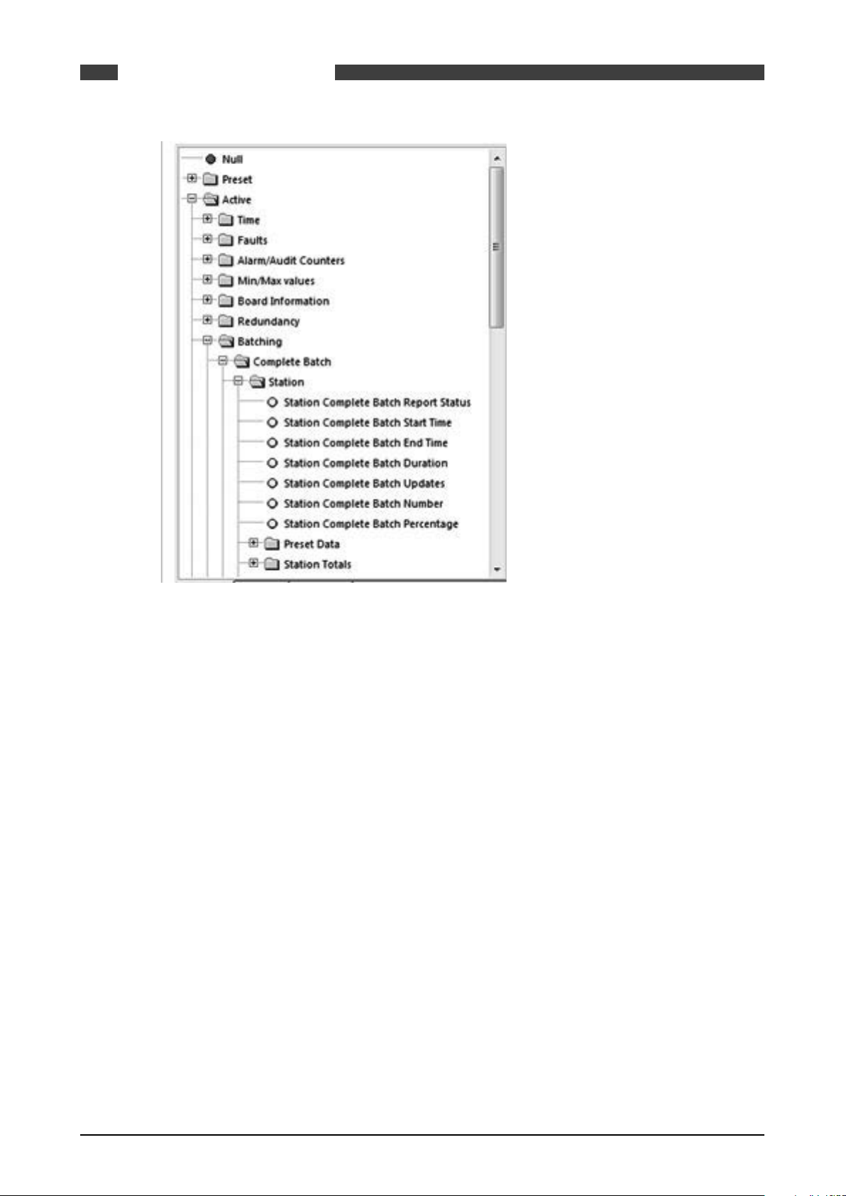
SUMMIT 8800GENERAL INFORMATION02

Figure 1 Example ID Tree

This is referred to as the ID tree which, depending on its context, includes folders and several parameters:

2.4.1 Type of data

The rest of this chapter will explain the folders available, the type of selection within the folder and any other corresponding data.

Preset Data

Essential to the conﬁguration of the ﬂow computer. Typical data would be keypad values, operating limits, equation selection, calibration data for Turbines and Densitometers and Oriﬁce plates. This data would be present in a conﬁguration report, and enables you to see what the ﬂow computer is conﬁgured to do. Used for validation and will form the Data Checksum (visible on the System Information Page). E.g., if a data checksum changes, the setup of the ﬂow computer has changed and potentially calculating different results to what is expected. Typically conﬁgured and left alone, only updated after validation e.g. every 6 month / 1 year.

Active Data

These values cover inputs to the ﬂow computer. E.g., from GC, pressure & temperature transmitters, meters etc.. Also Values calculated in the ﬂow computer. E.g., Flow rates, Z, Averages, Density etc..

Local Data

Data that an operator can change locally to perform maintenance tasks. E.g., turn individual transmitters off without generating alarms. Setting Maintenance mode or Proving Mode.

18 www.krohne.com 08/2013 - MA SUMMIT 8800 Vol2 R02 en

Page 19

SUMMIT 8800

Totals

Totals for the streams and station. Contents of this folder are stored in the non-volatile RAM and are protected using the battery.

Custom

User deﬁned variables. Allows calculations, made in a LUA script, to be used in a conﬁguration. For details, see volume 3.

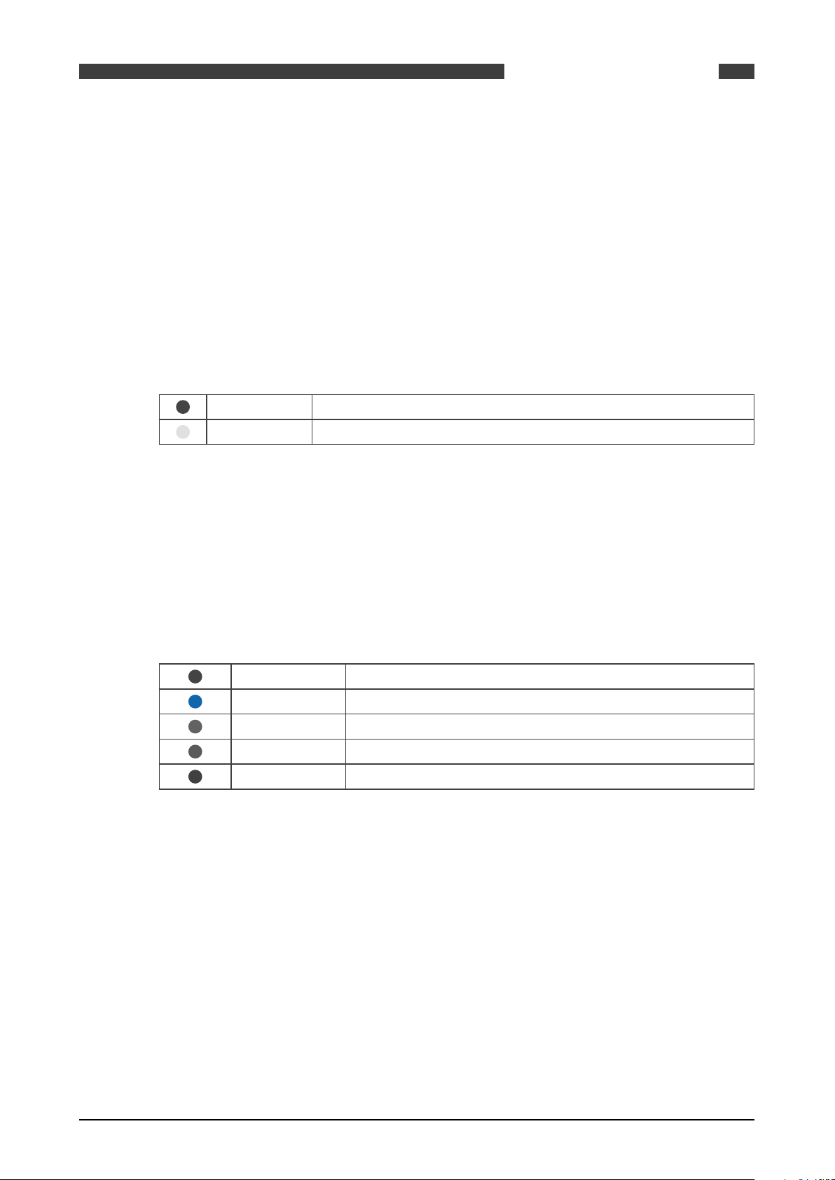
2.4.2 Colour codes

With each parameter and option, there are corresponding coloured dots that represent the access and status of the particular selection.

General ID tree

Please note that it might be possible to change the values via the screen

GENERAL INFORMATION

Red Dot Data is Read/Write and can be changed over Modbus.

Yellow Dot Data is Read-Only and cannot be changed over Modbus

90% of the data will be Read Only, but items such as Serial Gas Compositions, Time/Date, MF are commonly written over Modbus.

NOTE: Although the ID may be read/write, the security setting determines whether the ID indeed can be written.

Alarm Tree

The alarm tree is built of all the registers that hold alarm data. Alarm registers are 32-bit integers, where each bit represents a different alarm.

Red Dot Represents an accountable alarm visible on the alarm list.

Dark Blue Dot Represents a non-accountable alarm visible on the alarm list.

Orange Dot Represents a warning visible on the alarm list.

Light Blue Dot Represents a status alarm, not visible on the alarm list.

Black/Grey Dot Represents a hard- or software fault alarm visible on the alarm list.

An example of typical usage would be the General Alarm Register. This is a 32 bit register that indicates up to 32 different alarms in the ﬂow computer. This will contain Status Alarms, for example, 1 bit will indicate if there is a Pressure alarm or not. If the Pressure Status bit is set the user will know that there is a problem with the Pressure. This should be sufﬁcient information, however if it is not satisfactory, the user can look at the Pressure alarm, this contains 32 different alarms relating to the Pressure measurement, these would be Red Dots as they each can create an entry in the alarm list. By reading this register the user can view exactly what is wrong with the Pressure measurement.

The Light Blue Dots are generally an OR of several other dots. By reading the General register you can quickly see if the unit is healthy, more information can be provided by reading several more registers associated with that parameter.

08/2013 - MA SUMMIT 8800 Vol2 R02 en

www.krohne.com

Page 20

2.5 Speciﬁc Requirements for Meters and Volume Convertors

2.5.1 Numbering formats

The number formats used internally in the unit are generally IEEE Double Precision ﬂoating point numbers of 64 bit resolution. It is accepted that such numbers will yield a resolution of better than 14 signiﬁcant digits. In the case of Totalisation of Gas, Volumes, Mass and Energy such numbers are always shown to a resolution of 8 digits before the decimal point and 4 after, i.e. 12 signiﬁcant digits. Depending upon the required signiﬁcance of the lowest digit, these values can be scaled by a further multiplier.

2.5.2 Alarms

Each of the various modules that comprise the total operating software, are continuously monitored for correct operation. Depending upon the conﬁguration, the ﬂow computer will complete its allocated tasks within the conﬁgured cycle time, 250mS, 500mS or 1 second. Failure to complete the tasks within the time will force the module to complete, and where appropriate, a substitute value issued together with an alarm indication. For example, if a Calculation fails to complete correctly then a result of 1 or similar will be returned, which allows the unit to continue functioning whilst an accountable alarm is raised, indicating an internal problem.

SUMMIT 8800GENERAL INFORMATION02

2.5.3 Accountable alarm

When the value of any measurement item or communication to an associated device that is providing measurement item to the SUMMIT 8800 goes out of range, the ﬂow computer will issue an Accountable Alarm. When any calculation module or other item that in some way affects the ultimate calculation result goes outside its operating band, i.e. above Pressure Maximum or below Pressure minimum, then the SUMMIT 8800 will issue an Accountable Alarm.

When the SUMMIT 8800 issues an Accountable alarm a number of consequences will occur as follows:

Front panel accountable alarm will turn on and Flash. Nature of accountable alarm will be shown on the top line of the alarm log. Alarm log will wait for user acknowledgement of alarm. During the period of the alarm, main totalisation will occur on the alarm counters.

2.5.4 Optional consequences

Depending upon the conﬁguration of the SUMMIT 8800 the following optional Consequences will also occur:

An Entry will be made in the Audit Log, with Time and Date of occurrence. The “Used” value of the Parameter in Alarm will be substituted by an alternative value, either from an alternative measurement source that is in range, or from a pre-set value. A digital Alarm output will indicate an Alarm condition.

20 www.krohne.com 08/2013 - MA SUMMIT 8800 Vol2 R02 en

Page 21

SUMMIT 8800

METERING PRINCIPLES

3. Metering principles

In this Chapter the different meter technologies supported by the SUMMIT 8800 and the need for correction and normalization is described. Each of these technologies has its own particularities which are important to know when conﬁguring the ﬂow computer.

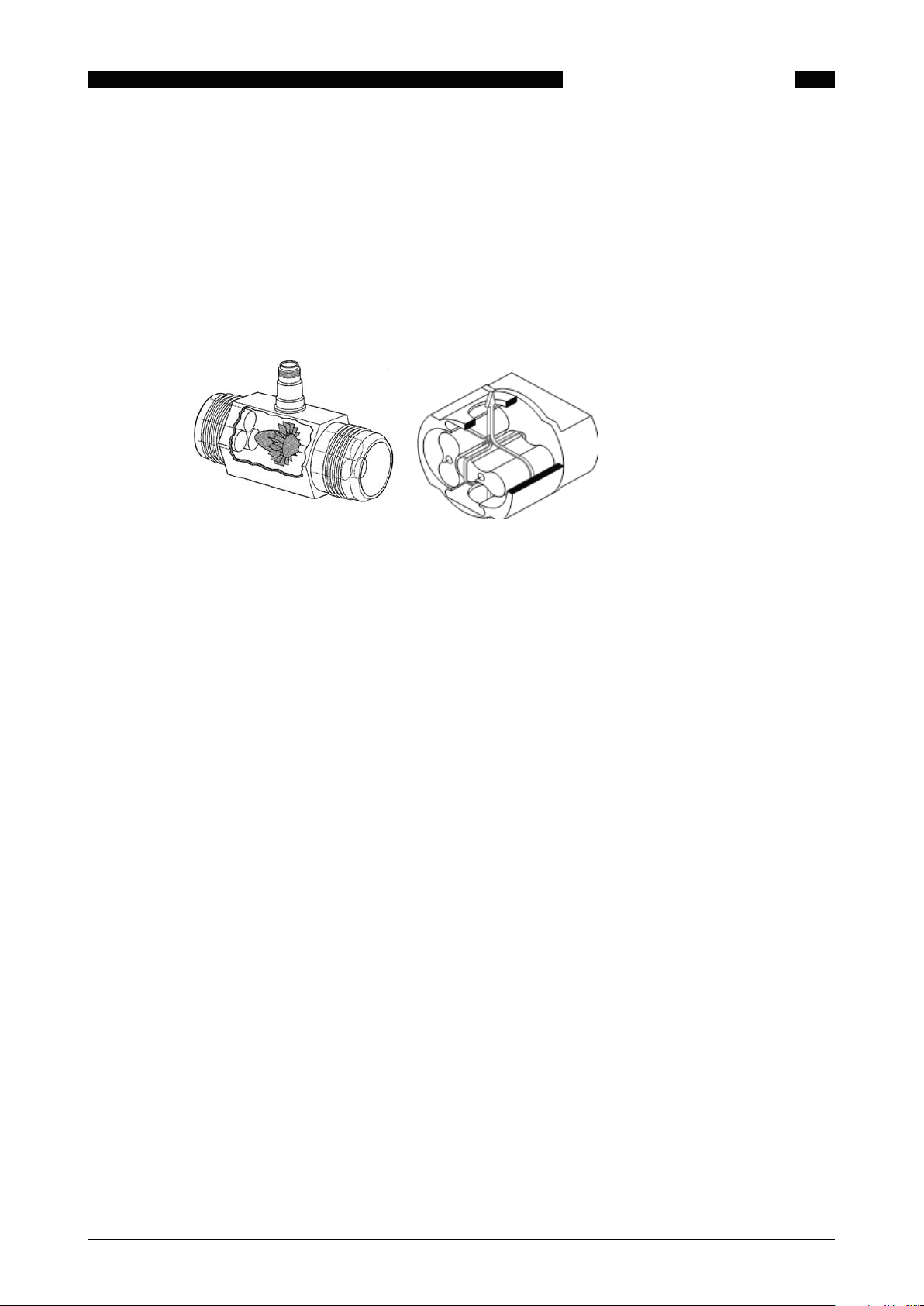
3.1 Pulse based meters: e.g. turbine/ positive displacement / rotary meter

This method stems from the time when rotating meters where used, such as turbine meters and rotary (Positive displacement) meters.

Figure 2 Turbine and rotary meter

A turbine meter is basically a fan in a tube. The gas makes the fan rotate and the rotations are recorded in an index on top of the meter. A positive displacement or rotary meter consists of two tighly coupled impellers which together create a moving chamber of gas. The rotation of the impellers drive an index.

A contact switch is operated by the rotating meter. The result is that the periodic closure of the switch is directly related to the amount of gas going through the meter. Depending on the location of the switch there are:

HF pulses or high frequency pulses

• The switch can be mounted just above the turbine blades. This switch is closing at the higher rate than the meter rotates (typically up to 5000 Hz). The ratio between the two is called “blade ratio”.

MF pulses or medium frequency pulses

• The switch mounted on the primary axes, so this switch is closing every turn of the meter. This results in a medium frequency pulse (typically up to 500 Hz)

LF pulses or low frequency pulses

• For low cost meters the switch can be mounted in the index after a gear resulting in slow pulsing switches and in a low accuracy measurement (typically below 50 Hz)

A problem with this method is that the switches do not always close 100% reliable. This is particularly true for the HF pulses as non-contact switches are used. This means that we can have missing pulses. Also too many pulses can occur, e.g. when interference occurs with the high frequency wires or due to thunder storms. The solution is to have dual pulses and check the relation between the two.

It may also be that a turbine blade may break off resulting in the wrong measurement. There is therefore a need for diagnostics. Several solutions have been implemented:

• The dual pulse method with a 90° angle between the two. This allows for diagnostics and even corrections for missing pulses. An API classiﬁcation level A to E is available (see below) for this.

• A second pulse from a turbine wheel with different blade angle.

08/2013 - MA SUMMIT 8800 Vol2 R02 en

www.krohne.com

Page 22

SUMMIT 8800METERING PRINCIPLES03

• A second lower frequency pulse, so a combination of HF with MF or LF. Off course the frequency ratio or blade ratio between the two pulses must be given.

API has a classiﬁcation on the quality actions taken on the pulses:

API level E is achieved solely by correctly applied transmission systems, criteria and recommended installed apparatus of good quality.

API level D system consists of manual error monitoring at methods of comparison, as used in Levels A through D.

API level C consists of automatic error monitoring for number, frequency, phase, and sequence and error indication at speciﬁed intervals.

API level B consists of continuous monitoring, with an error indication under all circumstances when impaired pulses occur.

API level A: consists of continuous veriﬁcation and correction given by the comparator.

Basically a non-issue for ﬂow computers

This means: Only 1 pulse is needed on the ﬂow computer.

This means: two pulses must be installed: the meter pulse and monitor pulse, which may be of different frequency (see frequency ratio)

This means two pulses of the same frequency must be installed: the meter and monitor pulse.

The major issue here is; the ﬂow computer has to correct when a wrong pulse occurs. This is quite advanced and is fully implemented in the SUMMIT.

Nowadays more and more electronics is incorporated into the meters, such as in ultrasonic and Coriolis meters. These meters normally emulate two high frequency pulses, to make them look the same as rotating meters from the installation standpoint. The ﬂow is calculated and a special pulse output is driven by the processor. Although the need for a second output pulse is diminished, most meters still carry them. API Level A is not really required.

There are also meters with smart indexes. Here the indexes values itself can be read by the ﬂow computer. The advantage is that the totals on the meters index are identical to the ﬂow computer totals. Also, if the ﬂow computer is replaced, the total will be automatically read. The communication is then digital and can be read via the serial port.

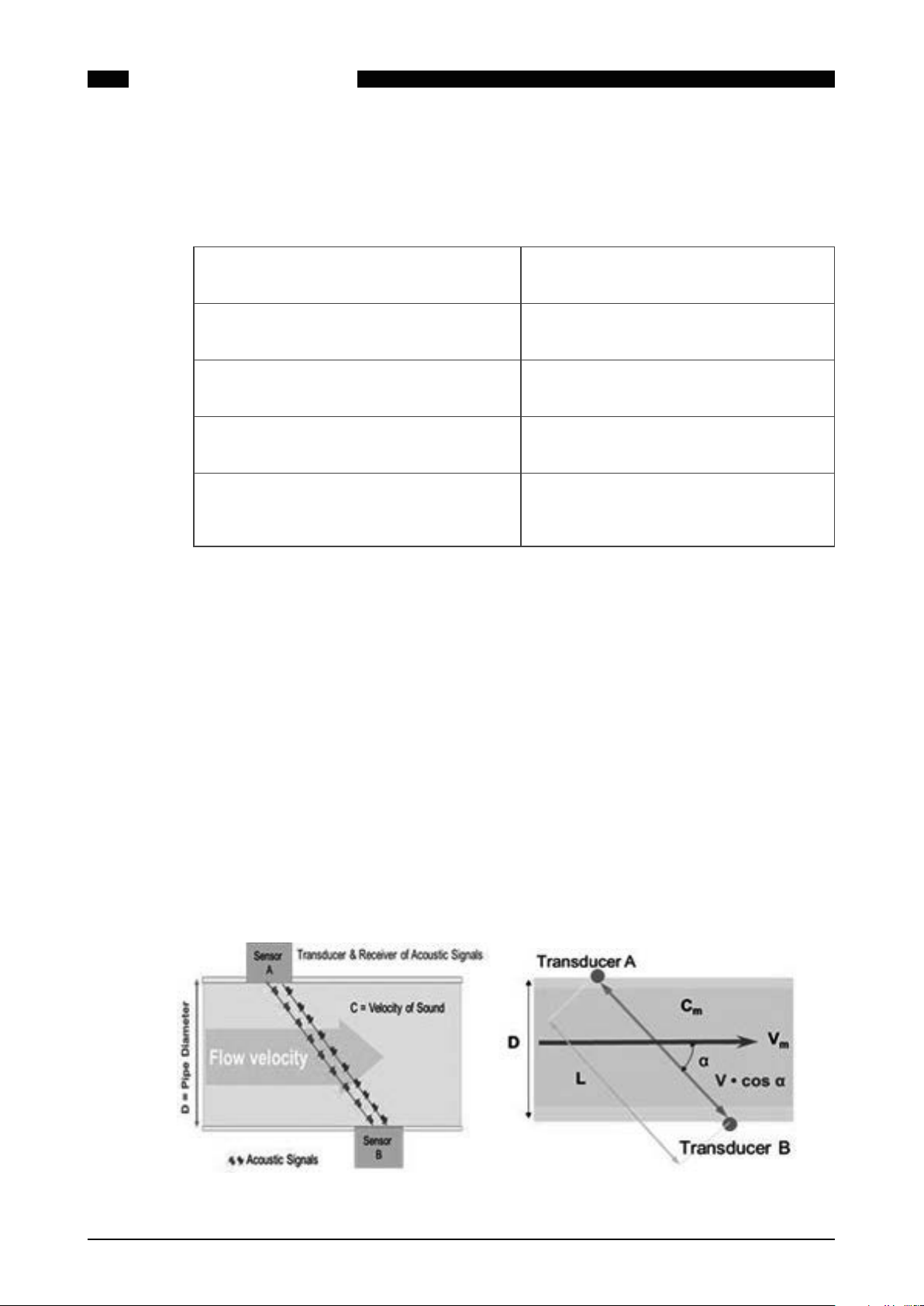
3.2 Ultrasonic meters

Ultrasonic meters are based on Transit Time Measurement of high frequency acoustic signals. These signals are transmitted and received along a diagonal measuring path. A sound wave going downstream with the ﬂow travels faster than a sound wave going upstream against the ﬂow. The difference in transit time is directly proportional to the ﬂow velocity of the liquid or gas. This can be compared with the speed a canoe travels upstream compared to downstream.

Figure 3 Ultrasonic measurement principle

22 www.krohne.com 08/2013 - MA SUMMIT 8800 Vol2 R02 en

Page 23

SUMMIT 8800

Mathematically, the time to transmit from a to b and back depends on the distance (L) between the two transducers, the speeds of the medium (v) and sound (c) plus the angle of the path (α) as follows:

Equation 1 Ultrasonic measurement formulae

With the velocity of the gas and the area of the pipe, the volume ﬂow rate can be calculated.

The problem is however that the oil or gas is not always equally distributed through the pipe. The ﬂow normally is faster in the centre than in at the pipe and has a certain proﬁle depending on turbulent or laminar ﬂow. So you do need the proper average velocity over the complete pipe. With single beam meters, such as clamp-on meters, the accuracy is therefore very limited. That is why the medium must be measured at different locations in the pipe. The trick is to best estimate the proﬁle/ the average ﬂow. All manufacturers come up with different arrangements in multi-path meters.

METERING PRINCIPLES

The output of ultrasonic meters is normally a combination of a dual pulse and a serial link.

• The dual pulse is generated by the electronics to emulate a turbine meter but does not provide its diagnostics.

• The serial link has typically a modbus protocol speciﬁc to the manufacturer, but for Instromet there is also the proprietary “Instromet protocol”. This serial protocol carries the ﬂow rate, but also meter diagnostics. For that reason in many cases both links are used at the same time.

Each manufacturer has its own set of diagnostics. Typical diagnostics are:

• The ampliﬁcation needed to send a signal between the transducers, both up- and downstream

• The signal to noise ratio at each transmitter

• The speed of sound measured by each path or ratio’s between them

• An indication of the type of ﬂow proﬁle

For gas there is an interesting additional diagnostics which is the calculated against the measured speed of sound based on AGA 10. The meter calculates besides the speed of the gas also the speed of sound. AGA 10 gives the formula from which the speed of sound can be calculated from the composition, the temperature and the pressure. Off course the measured and calculated speed of sound should be equal. If not one of the variables (meter, chromatograph or P or T) must be wrong or badly calibrated. This is therefore a perfect over all metering system check.

3.3 Differential pressure (dP) meters: e.g. oriﬁce, venturi and cone meter

Differential pressure ﬂowmeters use the Bernoulli’s rule to measure the volume ﬂow of gas or liquid in a pipe. They use a restriction in a pipe to measure the volume as it creates a difference in pressure before and after the restriction. The pressure difference (∆p) increases as ﬂow increases.

08/2013 - MA SUMMIT 8800 Vol2 R02 en

www.krohne.com

Page 24

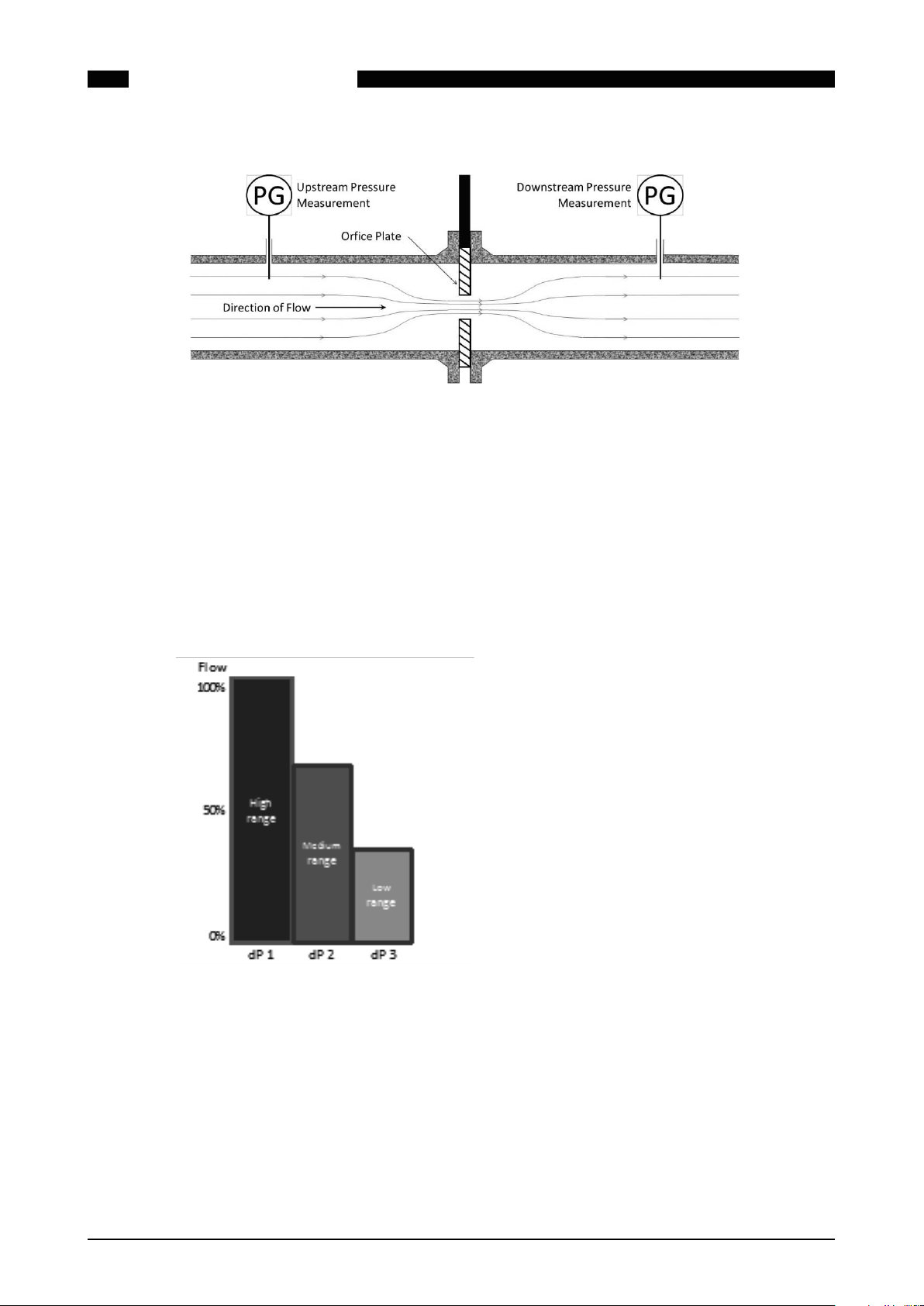
SUMMIT 8800METERING PRINCIPLES03

Figure 4 DP measurement principles

The shape of the restriction is determines the type of meter: oriﬁce, V-cone venture or nozzle (see later paragraphs). For each type there are several parameters that will be required to successfully calculate the ﬂow rate.

A single dP transmitter can used, but the problem is that a transmitter typically only has a 1:3 turndown ratio, so the accuracy for low ﬂow is very limited. For that reason in custody transfer applications multiple dP transmitters with different ranges are used for one meter and the ﬂow computer switches between them over depending on the ﬂow.

The SUMMIT can handle 1 to 3 ranges:

Figure 5 Up to 3 dP ranges

dP 1 will always measure the high range. In case of multiple ranges, an automatic switch-over to dP 2 will occur to medium range if the ﬂow decreases to the dP measurement range, optimizing the accuracy. If 3 ranges are available, dP 3 will kick in when the ﬂow gets within its measurement range. In the SUMMIT the switch-up and switch-down values for the dP may be given. They will be normally be different to have some hysteresis to prevent continues switch-up and –down when at the threshold.

In high end applications, where the accuracy is crucial, multiple dP transmitters per range can be used for the following reasons:

24 www.krohne.com 08/2013 - MA SUMMIT 8800 Vol2 R02 en

Page 25

SUMMIT 8800

• Accuracy: By averaging the transmitter values.

• Redundancy: If one transmitter fails, the other value may be used.

• Diagnostics: A warning can be given if there is a deviation between the transmitters.

For diagnostics 2 transmitters can be used, but it is not possible to determine which one is correct. For that reason 3 dP transmitters may be used. The SUMMIT also can have 1 to 3 dP transmitters for 1 to 3 ranges, so 1 to 9 dP transmitters in total.

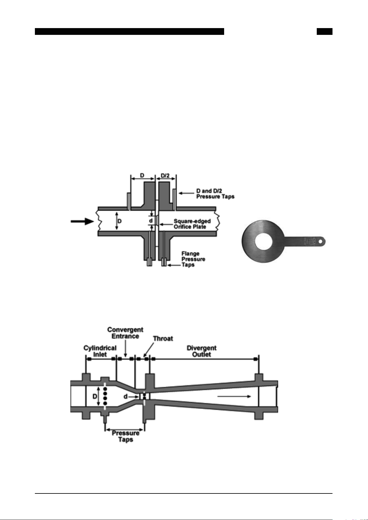
3.3.1 Oriﬁce Plate

A ﬂat circular plate with a hole, mounted inside the pipe that causes the ﬂuid to push through a smaller diameter.

METERING PRINCIPLES

Figure 6 Oriﬁce meter and plate

This is the most commonly used type of meter.

Classical venture or Herschel venturi Consists of a tapering in the pipe.

Figure 7 Venturi tube layout

08/2013 - MA SUMMIT 8800 Vol2 R02 en

www.krohne.com

Page 26

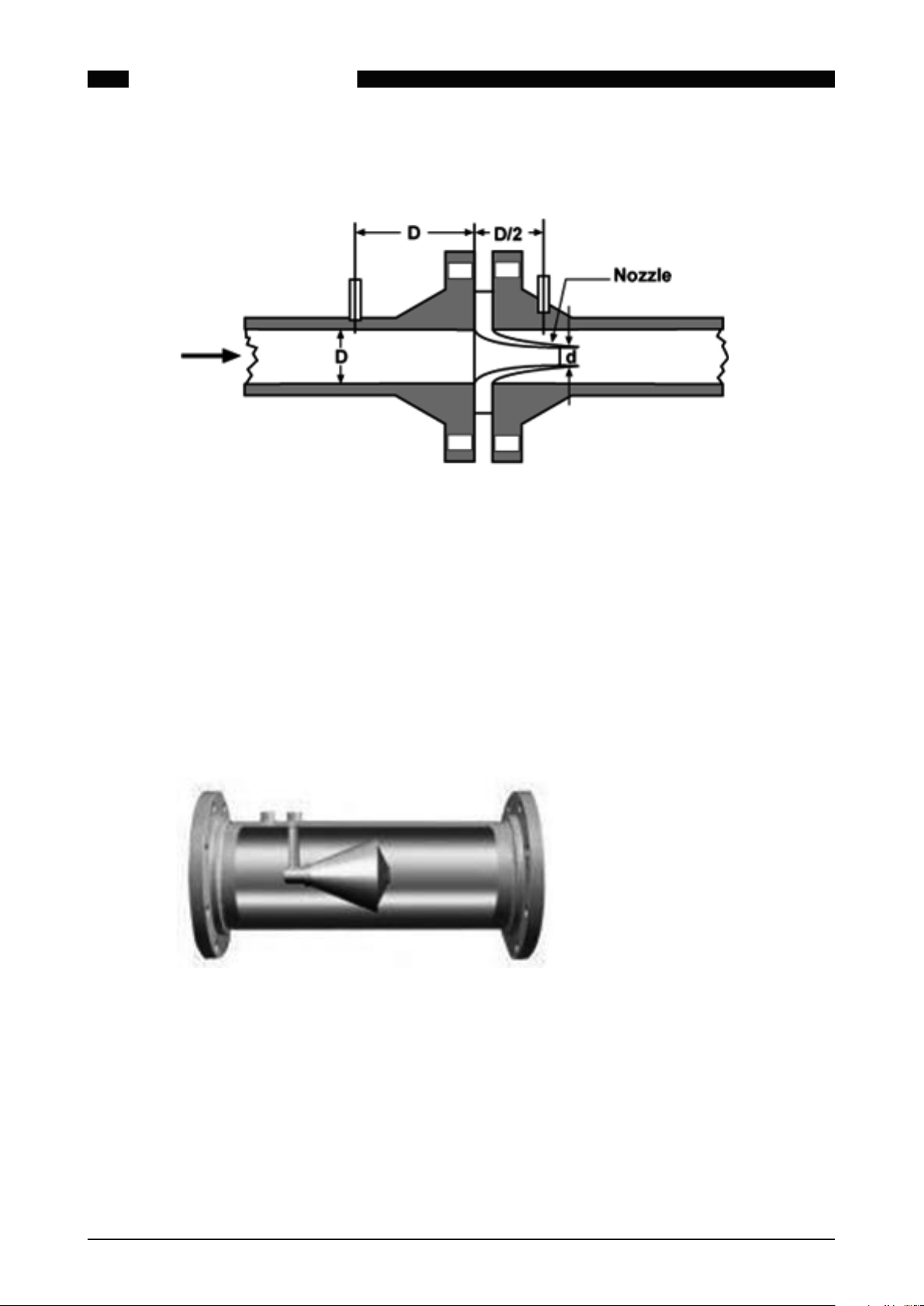
3.3.2 Venturi nozzle

The venturi nozzle has a trumpet shape restriction ending up in the pipe..

Figure 8 Venturi Nozzle

SUMMIT 8800METERING PRINCIPLES03

The main advantage of the venturi nozzle is pressure recovery.

ISA 1932 nozzle

Typically used for high velocity, set by ISO 5167 to determine the ﬂow of ﬂuid.

Long radius nozzle

A variation of the ISA 1932 nozzle, with a convergent section as the ISA 1932 nozzle and divergent section as a classical venturi

Cone or V-cone meter

The shape of the cone is to stable the ﬂow proﬁle in order to accurately measure the ﬂuid regardless of ﬂow properties.

Figure 9 V-cone meter

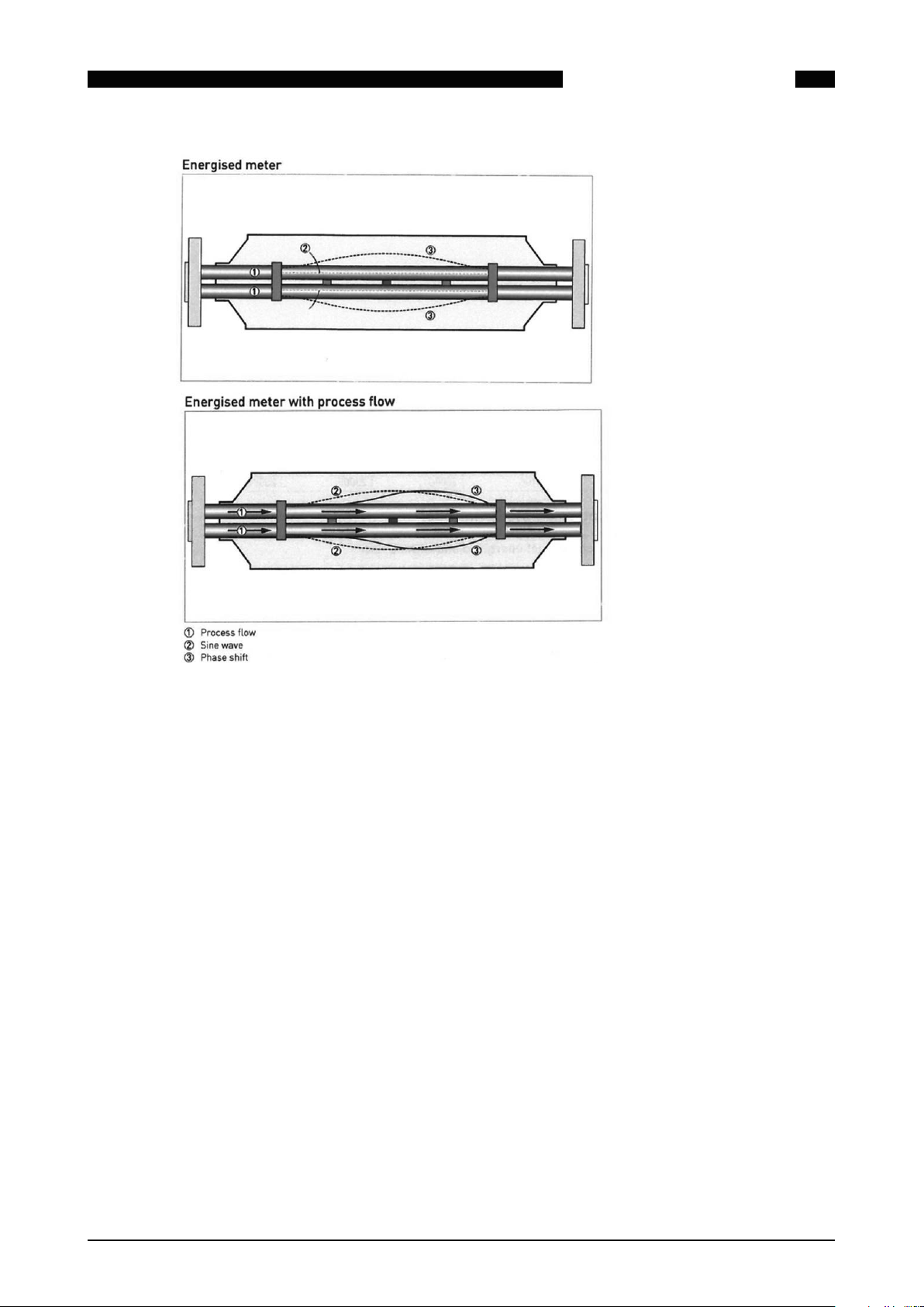
3.4 Coriolis meters

The Coriolis effect is the deﬂection of a ﬂuid by a rotating effect. If the rotation is clockwise, the deﬂection is to the left, if counter-clockwise, the deﬂection is to the right. Coriolis meters use a vibrating meter tube to generate the rotating effect and measure the deﬂection to calculate the mass passing through the meter.

26 www.krohne.com 08/2013 - MA SUMMIT 8800 Vol2 R02 en

Page 27

SUMMIT 8800

METERING PRINCIPLES

Figure 10 Coriolis meter ﬂow principle

A tube with a ﬂuid is brought into a sine waveform vibration. The eigen frequency with which this occurs is directly dependent on the density of the ﬂuid. If the ﬂuid is ﬂowing, a phase shift of the vibration will occur between the inlet and outlet of the tube. This phase shift is a measure of the velocity with which the ﬂuid passes through the pipe.

Traditional Coriolis meters have a bent tube to maximize the Coriolis effect. With more advanced electronics nowadays there is also straight tube Coriolis meters (see drawing).

Coriolis meters determine the mass ﬂow, but can also determine the density. Most Coriolis meters will also calculate the volume ﬂow using internal temperature and pressure, but it is recommended to use external measurements because of accuracy.

Coriolis meters typically have a dual pulse output mostly with the choice to have mass or volume ﬂow rate, where mass ﬂow rate is more accurate. Because of the fact that also density, pressure and temperature are available, most meters have also the option for a serial (modus) output, or a (multi-variable) Hart output.

08/2013 - MA SUMMIT 8800 Vol2 R02 en

www.krohne.com

Page 28

3.5 Meter corrections

3.5.1 Gas & steam

The meter provides a number of pulses/s. We would like to know the Volume ﬂow rate e.g. m3/s. For this need:

Pulse factor or impulse factor or meter factor

The factor provided by the manufacturer of the meter giving the number of pulses per volume of gas e.g. Pulses/m3. This assumes a linear meter. This is conﬁgured in the meter section.

Linearisation/ error Curve

The errors in % obtained during calibration of a meter which are the corrections needed to linearise the meter. So for each ﬂow rate a different error is used. In between the given ﬂow rates a linear interpolation is used. For ﬂow outside the operating range, extrapolation is used, except when MID is chosen, then the error is ﬁxed, and low and high ﬂow is used.

Volume ﬂow rate= Pulses per period*(1-Error) Gross Volume= Pulses*(1-Error)

SUMMIT 8800METERING PRINCIPLES03

3.5.2 Liquid

The meter provides a number of pulses/s. We would like to know the Volume ﬂow rate e.g. gallons/s. For this there are three important corrections for the meter possible:

K-factor

The factor provided by the manufacturer of the meter or as a result of proving which is the number of pulses per volume of ﬂuid e.g. Pulses/gallon. For a linear meter only one factor can be given. In case that the meter is not linear then a K-factor curve can be used. In this These factors are obtained during calibration or prove of a meter which are the corrections needed to linearise the meter. This is expressed by a variation of the K-factor over the speciﬁed ﬂow range. So for each ﬂow rate a different K-factor is used. In between the given ﬂow rates a linear interpolation is used. For ﬂow above maximum extrapolation is used.

Meter factor

The factor determined during proving to correct a ﬂuid ﬂowmeter for the ambient conditions by shifting its curve. The factor is used to compensate for such conditions as liquid temperature change and pressure shrinkage and is meter and product dependent. The meter factor should be close to1.

Equation 2 Volume calculation with MF

Equation 3 Gross volume calculation with MF

28 www.krohne.com 08/2013 - MA SUMMIT 8800 Vol2 R02 en

Page 29

SUMMIT 8800

3.6 Liquid normalisation

As with gas also oil ﬂow is measured by meters using a variety of different measurement principles, most based on volume ﬂow, some based on mass ﬂow. Examples are turbine meters, oriﬁce meters, Coriolis meters and ultrasonic meters. In all cases the line ﬂow is measured. The problem with this is that two measurements in the same pipe cannot be compared, due to difference in temperature, (to a lesser extend) pressure and possibly the type of product. This also means that billing of the oil will not be possible as no ﬁxed tariff can be applied.

For this reason a ﬂow computer is used to “normalize” the oil ﬂow to standard (or base) conditions, such as:

Temperature 15 or 20 oC or 60 oF

Pressure 1.01325 bar or 14.73 psi

So from the input density, the standard density is calculated by correcting for pressure and density. Then, from the standard density, the meter density is calculated, by again correcting for pressure and density.

METERING PRINCIPLES

Figure 11 Density calculations for oil

08/2013 - MA SUMMIT 8800 Vol2 R02 en

www.krohne.com

Page 30

The following formula applies:

Where ρm Line density of the liquid at metering conditions in kg/m3 or lbs/ft3 ρtp Line density of the liquid corrected for temperature and pressure in kg/m3 or lbs/ft3 ρs Standard Density of Liquid in kg/m3 or lbs/ft3 CTLρ : Temperature correction factor density at density test point CPLρ : Pressure correction factor density at density test point CTLm : Temperature correction factor at the meter CPLm : Pressure correction factor at the meter

Several different calculations, depending on the type of product, are available to determine the correction factors.

3.6.1 Mass and energy

SUMMIT 8800METERING PRINCIPLES03

The mass and energy can be calculated from the volume (or the volume from the mass) using:

Mass ﬂow rate: qm= qbc* ρm Energy ﬂow rate: qe= qn* Hs

Where Hs is the heating value. Two types can be used:

• The superior heating value, also known as higher heating value or higher caloriﬁc value or gross caloriﬁc value represents the heat released when a unit mass or volume of a material at 1 bar pressure and 25 °C is completely combusted and the combustion products are brought back to the starting pressure and temperature.

• The inferior heating value, also known as lower heating value or lower caloriﬁc value or net caloriﬁc value. This quantity assumes that the water produced by combustion remains in the vapour phase in the exhaust, and is lower than the gross caloriﬁc value by the latent heat of condensation joules/gram) of water at 25°C multiplied by the concentration of water in the material (expressed as grams/gram of fuel). For most common fuels, the net caloriﬁc value is about 10% less than the gross caloriﬁc value.

3.7 Gas normalisation

Gas is a compressible ﬂuid, due to this fact the reference conditions (P base and T base) on which the volume is calculated has to be given, which are normally contractually agreed.

Gas ﬂow is measured by meters using a variety of different measurement principles, most based on volume ﬂow, some based on mass ﬂow. Examples are turbine meters, oriﬁce meters, Coriolis meters and ultrasonic meters. In all cases the line ﬂow is measured. The problem with this is that two measurements in the same pipe cannot be compared, due to difference in temperature, pressure and possibly the composition of the product. This also means that billing of the gas will not be possible as no ﬁxed tariff can be applied.

For this reason a ﬂow computer is used to “normalize” the gas ﬂow to standard (or base) conditions, such as: Temperature 0, 15 or 20 °C or 60 °F Pressure 1.01325 bar or 14.73 psi

30 www.krohne.com 08/2013 - MA SUMMIT 8800 Vol2 R02 en

Page 31

SUMMIT 8800 CONFIGURATOR

We can calculate how much measurements may change to result in 1% change in normalized volume. Some typical numbers:

• The Volume changes 1% when the pressure changes 1% (e.g. 10 mBar at 1 bar)

• The Volume changes 1% when the temperature change of 3 °C

• The Volume changes 1% when the density change due to pressure or temperature:

• Pressure change of 4 bar or temperature change of 70 °C in a 5 bar pipeline

• Pressure change of 4 bar or temperature change of 4 °C in a 60 bar pipeline

• The Volume changes 1% when the density change due to composition:

• Either 3 % change of methane, 1% change of ethane or 0.5% change of pentane

This means that in gas:

• Correction for Pressure and Temperature is always needed.

• Correction for density is important for high pressure

• Correction for composition is only needed for high pressure

• A Gas chromatograph is only needed for changing composition

The SUMMIT 8800 ﬂow computer calculates the gas volume at these expanded conditions based on the measured actual ﬂow. For this the pressure and temperature at the location of the meter are used to calculate ﬂow at “normalised” or “standardised” conditions.

Since most gases are non-ideal gasses, the gas compression needs to be corrected by means of the compressibility factor (z-equation). This compressibility factor must be calculated at normal conditions and on line conditions, the division of these deﬁnes the correction for a non-ideal gas. This correction factor can also be determined based on the density determined at base conditions and at line conditions.

Many different formula’s have been developed in the last years to correct the liquid, gas and steam, depending on the type of product. Some based on a database of gasses, some based on physical properties, all off them with limited range of validity and associated accuracy. Therefore the conﬁguration of a ﬂow computer assumes the basic knowledge of formula’s needed. Here the basics:

3.7.1 Equation of state

As gas, the inﬂuence can be calculated from “Equation of state” P*V = n*Z*R*T or V =n* Z*R*T/P where: P = Pressure V = Volume n = Number of moles= mass/molar mass or n=m/M Z= Compressibility of the gas R = Universal gas constant = 8.31451 J/mol K T = Temperature

Z depends on the composition of the gas and is at very low pressure equal to 1.

From here it follows that: Vb= Vm* (Pm*Zb*Tb)/(Pb*Zm*Tm)

This is one of the ways to calculate the volume at base conditions. In this case the compressibility could be derived from the composition of the gas e.g. from a GC.

08/2013 - MA SUMMIT 8800 Vol2 R02 en

www.krohne.com

Page 32

3.7.2 Line and base density

An alternative way is to rewrite the equation in terms of density as the density of gas is ρ = m/V

The result is therefore: P = ρ *R/M*T or P = ρ*Rspeciﬁc*T

Therefore Vb= Vm* ρm/ ρb

This version can be used when the meter or line density is measured, e.g. when using a densitometer. The base density will typically be calculated using the AGA 8 formula or via the relative density/ speciﬁc gravity.

3.7.3 Relative density/ speciﬁc gravity

The terminology speciﬁc gravity is mostly used in US related speciﬁcations. This is referred to as ratio between gas density and air density.

In the rest of the world this is called relative density, where speciﬁc gravity is the density ratio between a ﬂuid and water. In this document it is further referred to relative density.

SUMMIT 8800CONFIGURATOR04

The base density can be derived from the relative density or speciﬁc gravity as follows:

The relative density or speciﬁc gravity is: db= ρb / ρair or ρb = db* ρair

The relative density can be calculated from the composition, e.g. via a GC

3.7.4 Mass and energy

The mass and energy can be calculated from the volume (or the volume from the mass) using:

Mass ﬂow rate: qm= qbc* ρm Energy ﬂow rate: qe= qn* Hs

Where Hs is the heating value. Two types can be used:

• The superior heating value, also known as higher heating value or higher caloriﬁc value or gross caloriﬁc value is referring to the energy produced when gas is burned and all ﬂue gases/vapours are cooled down to ie 1 bar pressure and 25°C.

• The inferior heating value, also known as lower heating value or lower caloriﬁc value or net caloriﬁc value.indicates the energy produced considering the burning of the gas without cooling down the vapours.

3.7.5 Enthalpy

Enthalpy is a measure of the total energy of a thermodynamic system and is important for steam. It includes the internal energy, which is the energy required to create a system, and the amount of energy required to make room for it by displacing its environment and establishing its volume and pressure.

As enthalpy cannot be measured, the enthalpy difference is normally used. It deals with the vapour of gaseous phases of liquid and is the energy required to turn the liquid into gases.

In most cases, the IAPWS or International Association for the Properties of Water and Steam is followed.

32 www.krohne.com 08/2013 - MA SUMMIT 8800 Vol2 R02 en

Page 33

SUMMIT 8800 CONFIGURATOR

3.8 Stream, station and batch totals

A total for ﬂow is calculated by multiplying the ﬂow rate by the time difference between the current and previous measurement. The SUMMIT 8800 keeps more than 25.000 different totals as a combination of:

Qty Type total Code used

2 Metric The totals in metric units

USC The totals in US customary units

2 Positive + Measured in positive direction

Negative - Measured in negative direction

11 Running totals Totals until now

Current period 15 minutes cqh. Totals for the running15 minutes

Current period Hourly ch. Totals for the running hour

Current period Daily cd. Totals for the running day

Current period Monthly cm. Totals for the running month

Current period Quarterly cq. Totals for the running quarter

Previous period 15 minutes

Previous period Hourly ph. Totals for the previous hour

Previous period Daily pd. Totals for the previous day

Previous period Monthly pm. Totals for the previous month

Previous period Quarterly pq. Totals for the previous quarter

pqh. Totals for the previous 15 minutes

9 Unhaltable U All product measured

Normal N Measured during normal

conditions

Error E Measured during error conditions

Maintenance M Measured during maintenance

Tariff level 1 t1 Measured when in tariff level 1

Tariff level 2 t2 Measured when in tariff level 2

Tariff level 3 t3 Measured when in tariff level 3

Tariff level 4 t4 Measured when in tariff level 4

Tariff level 5 t5 Measured when in tariff level 5

11 Pulse count Pulses The amount of pulses counted

Line volume VLine Line volume for the main pulse

Monitor volume VMon Line volume for the monitor pulse

Volume before normalisation

Volume after P/T correction

Normalised volume VN Normalised volume

Normalised volume net VNnet Net normalised volume (product

Vbc Volume after error curve

Vbc Volume after P and T correction

only)

08/2013 - MA SUMMIT 8800 Vol2 R02 en

www.krohne.com

Page 34

SUMMIT 8800CONFIGURATOR04

Normalised volume saturated

Energy E Energy ﬂow

Volume CO2 VCO2 CO2 ﬂow

Mass M Mass ﬂow

7 Stream 1 .1 .1 The totals for stream 1

Stream 2 .2 .2 The totals for stream 2

Stream 3 .3 .3 The totals for stream 3

Stream 4 .4 .4 The totals for stream 4

Stream 5 .5 .5 The totals for stream 5

Station A SA The totals for stream A

Station B SB The totals for station B

VNsat Normalised volume H2O saturated

The code for a running total of the positive unhaltable normalised volume of stream 1 is: +UVN.1 The code for a station A total of the current hourly period of the positive normal mass ﬂow is: SA+ch.NM

34 www.krohne.com 08/2013 - MA SUMMIT 8800 Vol2 R02 en

Page 35

SUMMIT 8800

3.9 Run switching

Run switching (also known as meter run staging or tube switching) is a function that allows the ﬂow of ﬂuid across multiple streams commonly used in stations and proving applications. The main purpose of this function is to maximize the station accuracy by trying to maximize the ﬂow through individual meters without exceeding their maximum.

Meters have a limited ﬂow range for which they work / work optimally. For minimum ﬂow their accuracy is limited, for maximum ﬂow there can be a chance for overspeeding, damaging the meter or limiting their accuracy. On the other hand stations have to deal with different ﬂow regimes, e.g. low ﬂow during summer, high ﬂow during winter. The solution is to have multiple meters with the total capacity for high ﬂow, while limiting the number of meters used during low ﬂow.

The run switch function in the SUMMIT is designed to do this automatically by switching valves to activate or deactivate streams within a station thus optimising the number of meters used for a certain ﬂow.

3.10 Proving

METERING PRINCIPLES

Proving is a function to determine and verify the accuracy of a stream ﬂow meter. With proving, the volume or mass ﬂowing through a meter is compared with the same ﬂow through the prover. As the prover is considered to be correct it is also referred to as the ‘known traceable volume’. The result of proving is the generation of a meter factor (MF) which is retro-applied to the ﬂow meter and which corrects the ﬂow meter to give the same reading as the prover.

The SUMMIT 8800 ﬂow computer can prove with the following prover systems:

• Unidirectional ball prover

• Bi-directional ball prover

• Piston small prover / compact prover

• Master meter

Historically provers are used in liquids while master meters are used for gasses. However nowadays, due to the complexity of provers, master metering is starting to get inroads into liquids too. In all cases, a prover / master meter is put in series with a meter under test to determine the accuracy of the meter.

Provers are based on a pipe with in it a ball or piston, moving with the medium. Detector switches are mounted at precise locations to detect the passing ball or piston. By very accurately determining the volume between detectors, the amount of volume moved from the prover to a meter can be determined and therefore the volume going through the meter. Since gas is compressible, this system is only working for liquids.

Master meters are meters with a higher accuracy that the meters to be tested. They are put in series with the meter under test. All the medium going through the master meter is also going through the meter under test.

Conventional ball provers typically generate enough ﬂow to get 10,000 or more meter pulses from the meter under test to successfully complete a prove cycle. Small volume provers due to size do not generate 10,000 pulses during a run cycle and are subject to pulse interpolation (double chronometry). Both types of provers are available as bi-directional and unidirectional.

08/2013 - MA SUMMIT 8800 Vol2 R02 en

www.krohne.com

Page 36

3.10.1 Unidirectional ball prover

TT PT

An inlet and outlet are connected to the pipework. A unidirectional prover only has ﬂow in one direction and the volume is based on the switching of the ﬁrst detector switch followed by the second with a passing sphere (displacer) used as a trigger.

SUMMIT 8800METERING PRINCIPLES03

Figure 12 Uni-directional prover

3.10.2 Bi-directional pipe prover

In a bi-directional prover the ﬂow can be reversed With the use of a four way diverter valve. The prove cycle is performed under operating stabilised conditions to maximize the accuracy.

Figure 13 Bi-directional prover

Key PT – Pressure transmitter in/outlet TT – Temperature transmitter in/outlet XS – Detector switches

36 www.krohne.com 08/2013 - MA SUMMIT 8800 Vol2 R02 en

Page 37

SUMMIT 8800

3.10.3 Small volume / piston provers

Small volume provers are available as compact or conventional pipe provers which use displacement to measure the volume and pulse interpolation.

METERING PRINCIPLES

Figure 14 Small compact prover

3.10.4 Master meter

In master metering a high accuracy master is put in series with other ﬂow meters to be tested while in production. This method of proving is predominately used for gas applications and is used in-line with the ﬂow meter being proved.

Figure 15 Master meter loop

08/2013 - MA SUMMIT 8800 Vol2 R02 en

www.krohne.com

Page 38

3.10.5 Proving procedure

A01: Start

Prove

command

issued

A02: Send the begin

prove command to the

required run

A03: Is the correct

frequency being

received?

A04: Begin prove

valve control

A05: Valves

correctly

positioned ?

A06: Flow

stabilisation

A07: Stabilisation

completed succesfully

A08: Prove

sequence

A10: Proving

sequence

completed ok ?

A13: Generate prove

report

A11: User accepts

KF/MF ?

A12: Update KF/MF

A14: Should

valves be reset ?

A15: End prove

valve control

A17: Send setpoints to

regular flow

A18: Send the end

prove command to the

required run

A19: Prove End

Yes

No Yes Yes

Yes

A16: Valves

correctly

positioned?

Yes

A09: Multi-point

prove?

Yes

Proving is a complex but well deﬁned procedure to control valves, take measurements and do calculations. As the quality of the result is depending very much on the tolerances, limits and stability of ﬂow, temperature, pressure and density they are very well checked and controlled during the proving cycle as deﬁned in many standards.

The following ﬂow charts illustrate the necessary procedure to successfully prove and implement the result. As the procedure is quite extensive, it is necessary to be able to track exactly what is happening. For that reason, a checklist is added with the parameters to check.

SUMMIT 8800METERING PRINCIPLES03

Figure 16 Proving ﬂowchart

38 www.krohne.com 08/2013 - MA SUMMIT 8800 Vol2 R02 en

Page 39

SUMMIT 8800

Proving description

A01 Start proving The proving request tag has been issued via display or Modbus - this

METERING PRINCIPLES

initiates the prove request

Tips: With the proving status tag, the result of the last prove can be monitored

• N/A

• OK

• Manually aborted

• Maximum runs reached

• Not enough runs remain

• Volume stability

• Pressure stability

• Temperature stability

• Valve setup error

• Valve return error

• Communications error

• Run error

• Volume deviation

• Pressure deviation

• Temperature deviation

• Density deviation

• Pressure alarm

• Temperature alarm

• Density alarm

• Frequency input

• Validation rejected

• Data update failed

• Valve error

• Turbine error

• Setpoint error

• USM error

With the proving position tag the status of the prove can be monitored Idle

• Beginning prove

• Initialising report

• Initialising communications

• Conﬁguring valves

• Stabilising ﬂow

• Running

• Resetting valves

• Ending communications

• Waiting for validation

• Generating report

The ball position tag does not indicate the actual ball position, but is a status indicator for the Proving run for ball provers. Instead of ball position monitor the status of the valve

A02 Send begin prove

command to required run

A03 Correct frequency? Prover frequency tag is checked if pulses are being received, thus

The proving.1 tag of the required stream is set.

The prover general alarm tag is set. These tags are displayed on the alarm page.

frequency cannot equal zero.

Conﬁrm that the pulse bus is conﬁgured correctly. Refer to section ‘prover I/O selection’ for conﬁguration details.

08/2013 - MA SUMMIT 8800 Vol2 R02 en

www.krohne.com

Page 40

SUMMIT 8800METERING PRINCIPLES03

A04 Begin prove valve

control

A05 Valves correctly

positioned?

A06 Flow stabilisation Volume, temperature, and pressure are checked for deviations.

A07 Stabilisation completed

successfully?

All conﬁgured valve are set to proper position. If conﬁgured the following valves are set in the following sequence.

1. Set run ﬂow control;

2. Open required run outlet;

3. Open prover outlet;

4. Set prover ﬂow control;

5. Close all run prover inlet;

6. Open required run prover inlet;

7. Close run outlet;

8. Set 4-way valve to reverse, only for ball provers;

9. Start ﬂow control.

Valve status tags can be found in the following location.

All conﬁgured valves are check if they are in the proper position with valve position tag.

1. Idle

2. Opening prover outlet valve

3. Opening prover ﬂow control valve

4. Positioning fourway valve

5. Opening run prover inlet valve

6. Closing run prover inlet valve

7. Opening run ﬂow control valve

8. Opening run outlet valve

9. Closing run outlet valve

10. Start regulating

11. Checking run outlet valves

12. Returning piston

13. Opening master run outlet

14. Closing master run outlet

• Minimum stability duration, this is the waiting time before stability check;

• Maximum stability duration, after this time the conditions must be stable;

• Stability limit, the maximum limit for the deviation.

Check is made if previous steps were successful.

Important: If successful the conditions are recorded and monitored throughout the proving.

For reference the standard deviation tag for ﬂow, temperature and pressure can be found under the following location.

There are a set of deviation alarm tags that are set is the standard deviation is greater than the limit set. Active>prover>alarms>live>prover pressure-temperature-ﬂow

A08 Proving sequence In this step sub routine proving sequence is initiated. The result of the

sequence can be successful or failed

A09 Multi-point prove? A check is made on how the prover is conﬁgured, single point or multi-

point.

If the prover is conﬁgured as multi-point proving, then the routine will go back to step A06 ‘ﬂow stabilisation’ and set the conﬁgured ﬂow rate for each proving point. If the prover is conﬁgured as single point proving, then the routine will continue to the next step.

40 www.krohne.com 08/2013 - MA SUMMIT 8800 Vol2 R02 en

Page 41

SUMMIT 8800

METERING PRINCIPLES

A10 Proving sequence

completed?

A11 User accepts KF/MF? Veriﬁcation made if user accepts new KF/MF.

A12 Update KF/MF If the previous step was accepted, then the new KF/MF is updated. The

A13 Generate prove report The proving status tag and other tags are updated.

A14 Reset valves? If the prove is successful the valves will be reset.

A15 End prove valve control All conﬁgured valves are set to the position to ﬁnish the prove. If

A16 Valves positioned

correctly?

A17 Send setpoints to

regulate ﬂow

A18 Send end prove

command to required run

A19 Prove end The prover general alarm tag is reset.

A check is made if ‘proving sequence’ was completed successfully, the ‘abort proving’ tag can be monitored.

• No

• Manual abort

• Valve failure

• Communications failure

• Run failure

• Pressure failure

• Temperature failure

• Density failure

• Volume failure

• Deviation during prove

• Turbine failure

• USM failure

The new K-factor and meter factor must be accepted through the validate results tag via the display or Modbus.

tags are calculated K and calculated MF.

If the prove fails the valves will not be reset and will stay in the same position.

conﬁgured the following valves are set in the following sequence.

1. Set 4-way valve to reverse, only for ball provers;

2. Set prover ﬂow control;

3. Open prover outlet;

4. Open run ﬂow control;

5. Open required run outlet;

6. Close prover inlet;

All conﬁgured valves are check if they are in correct position.

Send setpoints to regulate ﬂow

The proving.n tag of the required stream is reset.

3.10.6 Meter factor and K – factor

After every successful prove process, a ﬂow meter will be assigned a new meter factor (MF) and K- factor.

K- factor, the number of signal pulses from a meter during a prove divided by the actual corrected prover volume.

K-factor = (meter pulse)/(correct prover volume)

Meter factor, the value obtained by the corrected prover volume divided by the actual liquid volume passed through the ﬂow meter

MF = (correct prover volume )/(meter registered volume)

Equation 4 KF & MF prover calculation

08/2013 - MA SUMMIT 8800 Vol2 R02 en

www.krohne.com

Page 42

3.10.7 Proving sequence

B01: Begin Prove

sequence

B09: Maximum runs exceded?

B10: Too many

consecutive bad

runs ?

B11: Is the error

recoverable?

B07: Run completed

ok?

B08: Enough good

consequtive runs with

required repeatability

B13: Sequence

succesfull

B12: Sequence

failed

Yes

YesNo

Yes

B06:

Proverrun

B02: Allow

regulate?

B03: Flow

stabilisation

B04: Stabilisation

completed

succesfully ?

Yes

B05: Check current conditions have not

deviated from the

start of prove

SUMMIT 8800METERING PRINCIPLES03

42 www.krohne.com 08/2013 - MA SUMMIT 8800 Vol2 R02 en

Figure 17 Proving sequence ﬂowchart

Page 43

SUMMIT 8800

Description

B01 Start proving sequence The proving sequence sub-routine is initiated by the main

B02 Regulate control valves? Release PID between runs’. If yes, then the control valve will

B03 Idem A06

B04 Idem A07

METERING PRINCIPLES

prove routine. The results of the individual run are stored in the status.run’n’ tag.

A general ﬂag is set or reset, this done on the proving sequence tag.

be released, and continue to the next step to stabilise ﬂow again.

Flow stabilisation Volume, temperature and pressure are checked for

deviations.

Minimum stability duration, this is the waiting time before stability check; Maximum stability duration, after this time the conditions must be stable; Stability limit, the maximum limit for the deviation.

Stabilisation completed successfully?

Check initiated if previous step was successful. Important: If successful the conditions are recorded and monitored throughout the proving process.

B05 Check deviation of

conditions

B06 Proving run

For reference the standard deviation tag for ﬂow, temperature and pressure can be found under the following location.

There are a set of deviation alarm tags that are set is the standard deviation is greater than the limit set.

Volume, temperature and pressure are checked for deviations from the start of the prove.

This step is depended on the type of prover conﬁgured. Depending on the selection, a sub-routine is started.

Refer to prover>prover options>general>prover type

Ball prover (tag: ball position)

• Idle

• Initialising switches

• Waiting for initialisation

• Forward rotate 4 way valve

• Forward counting pulses

• Forward waiting chamber

• Initialising switches

• Waiting for initialisation

• Reverse rotate 4 way valve

• Reverse counting pulses

• Reverse waiting chamber

• Generating report

Master meter (tag: run position)

1. Idle

2. Initialising switches

3. Waiting for initialisation

4. Starting run

5. Counting Pulses

6. Ending run

7. Ending run

8. Generating report

08/2013 - MA SUMMIT 8800 Vol2 R02 en

www.krohne.com

Page 44

Small volume prover (tag: piston position)

• Idle

• Initialising piston

• Initialising switches

• Waiting for initialisation

• Releasing piston

• Counting pulses

• Returning piston

• Generating report

B07 Run completed ok? Check if the run is completed successfully.

B08 Check consecutive run and

repeatability

B09 Maximum runs exceeded? Check if maximum runs are exceeded.

B10 Too many consecutive bad

runs?

B11 Is error recoverable? Is error recoverable? recoverable error are:

B12 Sequence failed Sequence failed.

B13 Sequence successfully Sequence successfully.

Check is done if enough consecutive runs required is completed successfully. Settings repeatability or uncertainty

Check if too many consecutive bad runs are performed

Valve errors Accountable alarms

SUMMIT 8800METERING PRINCIPLES03

44 www.krohne.com 08/2013 - MA SUMMIT 8800 Vol2 R02 en

Page 45

SUMMIT 8800

C02: Rotate 4way

valve forward

C03: Valves

correctly

positioned ?

C19: Enough

pulses received?

C20: Run Completed

Succesfull

Yes

C01: Start Run

C04: Dectector

switch1 triggered

C05: Start counting

pulses

C06: Dectector

switch2 triggered

C07: Stop counting

pulses

C08: Wait for ball to reach chamber

C10: Rotate 4way

valve reverse

C11\: Valves

correctly

positioned ?

Yes

C12: Dectector

switch2 triggered

C13: Start counting

pulses

C14: Dectector

switch1 triggered

C15: Stop counting

pulses

C16: Wait for ball

to reach chamber

C17: Calculate pulses

C18: Release all flow

control valves

C22: Run Completed

Un-Succesfull

C21: Release all flow

control valves

C09:

Run timer timeout

alarm active ?

Yes

3.10.8 Proving run (ball position)

METERING PRINCIPLES

Figure 18 Proving run ﬂowchart

08/2013 - MA SUMMIT 8800 Vol2 R02 en

www.krohne.com

Page 46

Description

C01 Start Run

C02 Rotate 4 way valve forward

C03 Are valves correctly positioned? If not abort run (jump to C21)

C04 Detector switch 1 triggered

C05 Start counting pulses

C06 Detector switch 2 triggered

C07 Stop counting pulses

C08 Wait for ball to reach chamber

C09 Run timer timeout activate? If so abort run (jump to C21)

C10 Rotate 4 way valve reverse

C11 Valves correctly positioned?

C12 Detector switch 2 triggered If not abort run (jump to C21)

C13 Start counting pulses

C14 Detector switch 1 triggered

C15 Stop counting pulses

C16 Wait for ball to reach chamber

C17 Calculate pulses

C18 Release all ﬂow control valves

C19 Enough pulses received? If not abort run (jump to C22)

C20 Run completed successfully

C21 Release all ﬂow control valves

C22 Run completed un-successfully

SUMMIT 8800METERING PRINCIPLES03

3.11 Sampling

Fixed time period Activated during deﬁned period with on and off timings

Duration Actived for a ﬁxed lenght of time

Batch Quantity measurement based on parcel size

Continuous Continuously running and obtaining samples

46 www.krohne.com 08/2013 - MA SUMMIT 8800 Vol2 R02 en

Page 47

SUMMIT 8800 CONFIGURATOR

4. The conﬁgurator

4.1 Applications

The SUMMIT 8800 is a multi-medium hydrocarbon ﬂow computer which can handle 5 streams plus prover for liquid, gas, and steam applications simultaneously. It has been designed to accommodate multi-stream utilising various different types of ﬂowmeter technology, and can be completely customised as per the user’s requirements. This includes the operational units to be US Customary (USC) or Metric units, but also includes batching, sampling, valve switching etc..

Many other conﬁgurations features including data changing screen- and print layout but also graphical illustrations can be conﬁgured and will be described in detail in volume 3 of this manual set.

Application summary

The SUMMIT can be conﬁgured for the following metering types:

• Gas Master Meter

• Liquid Prover

• Gas Turbine/ Positive Displacement (PD)

• Gas Ultrasonic

• Gas Differential Pressure (DP)

• Gas Coriolis

• Liquid Turbine

• Liquid Ultrasonic

• Liquid Differential Pressure (DP)

• Liquid Coriolis

• Steam Ultrasonic

4.2 Measurement devices and signals

The SUMMIT 8800 is capable of receiving various signals from different technologies, and communicating with various ﬁeld instruments including smart meters, and multi variable transmitters. A simple summary of the types of commonly available signals from various meters, transmitters and transducers that can be used in conjunction with the SUMMIT 8800:

• HART, 1 or 2 masters or burst mode, up to 3 transmitters, 4 variables

• PRT/RTD/PT-100, 3 or 4 wire.

• 0-20mA/ 4-20mA

• Serial communication, several protocols

• Digital inputs

• Pulse inputs

• Status inputs

The following signals can also be used by the SUMMIT 8800 to communicate and send signals to various types of PLC, DCS, HMi, SCADA and other systems, including writing to ﬁeld instrument registers

• 4-20mA output

• Serial communication, several protocols

• Digital outputs

• Pulse outputs

4.3 Create a new application

For initial installation and main menu functions of the software refer to Volume 1 of the handbook set.

08/2013 - MA SUMMIT 8800 Vol2 R02 en

www.krohne.com

Page 48

SUMMIT 8800CONFIGURATOR04

This volume limits itself to the ofﬂine editing functions of the conﬁgurator, speciﬁcally to the conﬁguration functions related to the meters and associated equipment. The ofﬂine function allows the user to create a new application without actually being connected to the ﬂow computer. It is also possible to load a previously created application from:

• a ﬂow computer by using “Connect”

• a disk by using “Load Setup”.

The SUMMIT is continuously being improved with new functions and capabilities resulting in different versions of the conﬁgurator. The conﬁgurator is upwards compatible: a new conﬁgurator can handle all previous versions. Off course, only the highest version has all the latest capabilities, so it is recommended to always use the latest version. The ﬂow computer must support the conﬁgurator capabilities. Its ﬁrmware must therefore be compatible to the conﬁgurator version used, if not, the application cannot be loaded into the ﬂow computer. It is possible to upgrade old applications to new versions via “Load setup” but check whether all functions are still supported.

To start the creation of a new application, start the conﬁgurator and select “Edit ofﬂine”:

Figure 19 Conﬁgurator main menu

And select the version to be used:

48 www.krohne.com 08/2013 - MA SUMMIT 8800 Vol2 R02 en

Page 49

SUMMIT 8800 CONFIGURATOR

Figure 20 Conﬁguration version

NOTE: The version must match the ﬁrmware loaded in the SUMMIT 8800. See Appendix 1: software versions.

In the SUMMIT 8800 it is possible to deﬁne one to ﬁve different streams (or runs) plus a prover. Each of these streams is independent from the other. Each can be any metering medium (gas, liquid or steam) and any meter type: turbine, ultrasonic, Coriolis, oriﬁce etc. (see next paragraphs for details). Also each stream can have a different engineering unit: Metric or USC (US Customary) or a mix of them. The prover can be a master meter, but for liquid it can also be a small volume (or compact) prover and a uni- or bidirectional prover.

For a new application select the ﬂow computer type (machine type). This will normally be “Standard”, but if proving is required select gas prover or liquid prover. Then select per stream, the type of metering; in this case a gas turbine and a liquid Coriolis.

Figure 21 Conﬁguration machine type

08/2013 - MA SUMMIT 8800 Vol2 R02 en

www.krohne.com

Page 50

4.4 Main Screen

The main conﬁguration page of the Conﬁgurator software provides all options available for the machine type selected. This means that certain menu options may not be available. For instance if only one meter and no prover is selected, only 1 stream will be shown and the prover and station tab will not be available.

SUMMIT 8800CONFIGURATOR04

Figure 22 Main Conﬁgurator screen

The summary page shows the memory consumption for setup and log and details in the Information box.

For the main functions Save/ print/ preview/ import/ download and help, see volume 1

This volume describes all functions related to the meters and associated equipment: The manual follows the sequence most commonly used during conﬁguration:

• Conﬁgure the hardware

• Conﬁgure the stream

• Conﬁgure the prover/ master meter if available

• Combine streams to a station if needed

• Optionally Conﬁgure valves, sampler and batching

In volume 3 the rest of the functions are described:

• Time and date

• Display

• Logging: Data, alarm and audit trail

• Reporting

• Communication

• Web access

• Miscellaneous functions

It is important to deﬁne ﬁrst what boards will be used and what signals will be used on each board.

50 www.krohne.com 08/2013 - MA SUMMIT 8800 Vol2 R02 en

Page 51

SUMMIT 8800 HARDWARE DETAILS

5. Hardware

This paragraph provides instructions on how to conﬁgure the I/O boards for the types of signals to be utilised by the ﬁeld instruments to the SUMMIT 8800. (For details on the boards, see volume 1)

Figure 23 Conﬁgurator I/O board setup

The SUMMIT 8800, I/O and communication boards can be conﬁgured on-line or off-line. When on-line, the slots will be populated as the current conﬁguration information will be polled by the software. When setting up in off-line mode, it is important to select the right I/O and communication board in the corresponding slot.

To conﬁgure a board, select the board type as per Figure 23, right hand side. This is done by clicking on the pull down menu and selecting the required/installed board in the relevant position.

Figure 24 I/O and communication board selected

Figure 24 shows an example where each slot is occupied different boards.

Directly below the Board Type is a Warning tab. Here can be conﬁgured what action should be taken if, during normal operation, a wrong, missing or faulty board is found. This can be a warning, a fault or no action at all.

08/2013 - MA SUMMIT 8800 Vol2 R02 en

www.krohne.com

Page 52

5.1 I/O board Conﬁguration

To conﬁgure a board, click on the desired board as it appears in Figure 24. The board is divided into sections for the different in- and outputs, visible only when hovering over section. Depending on the section clicked, the speciﬁc in- or output is selected. As an example, when clicking on the analog board in slot 3 section digital in, the digital inputs are selected for conﬁguration:

SUMMIT 8800HARDWARE DETAILS05

Figure 25 Board conﬁguration window

The top of the conﬁguration screen shows which board type and what slot position is choosen.

On the left side of the window there are different in- and outputs for conﬁguration with the selected one highlighted. Of course any other selection can then be made by clicking on the section. The different selections will be described in the following paragraphs.

On the right the associated pin numbers on the connector are shown.

The button marked with “< None >” signiﬁes what software variable is associated with the hardware signal connected. A software variable can be selected from an ID data tree. For each type of signal the tree will only be populated with appropriate variables to prevent mistakes. For instance in the case of a frequency input only the “active” and “custom” variables are available.

52 www.krohne.com 08/2013 - MA SUMMIT 8800 Vol2 R02 en

Page 53

SUMMIT 8800 HARDWARE DETAILS

Figure 26 Signal selection from a tree

Of course the variable selected must match the hardware signal associated with it (see volume

1). Only one variable can be assigned to one signal.

Although it is possible to assign the same variable to two signals, an unpredictable behavior will be the result. For this reason an error will be given when this is the case. Make sure to correct this mistake.

Figure 27 Error for a duplicated variable

5.1.1 HART Input

Most I/O boards have 1 or 2 Hart inputs (/loops), however the switch I/O board has none.

HART (Highway Addressable Remote Transducer) is a protocol, superimposed on the 4-20 mA signal, to connect smart transmitters to the ﬂow computer. Hart has the following characteristics:

• A transmitter can send 1 to 4 values via HART, but only the primary measurement may also be transmitted via 4-20 mA.

• Hart transmitters can be in multi-drop or in burst mode.

• Multi-drop: each transmitter gets an address between 1 and 15 and a master reads one transmitter after the other.

• Burst mode: only one transmitter is connected and has no address (address 0). The transmitter is continuously transmitting its data and multiple devices may be listing.

• Hart accepts 2 masters, typically a ﬂow computer and a ﬁeld communicator (for calibration in the ﬁeld). In redundancy mode two SUMMIT 8800 can communicate with one transmitter, but one has to be set as master 1, the other as master 2.

• One Hart loop can handle up to 15 devices in multi-drop. The SUMMIT 8800 limits this number to 3 to have an update time of less than 1 second.

The associated conﬁguration screen is as follows:

08/2013 - MA SUMMIT 8800 Vol2 R02 en

www.krohne.com

Page 54

SUMMIT 8800HARDWARE DETAILS05

Figure 28 Conﬁgure HART inputs

Select the HART loop required as loop 1 or 2. In “options” select in Master 1 or 2 or Burst mode. Please note that in burst mode only 1 transmitter can be chosen, the other transmitters are greyed out.. Set the number of retries and the timeout (in seconds) before an error must be generated.

Then for each transmitter set under “Conﬁgure Transmitter”:

• Assign a short id address: 0 when in burst mode, between 1 and 15 otherwise. Make sure the actual transmitters are programmed accordingly.

• Select the primary variable to be read from this transmitter from pull down tree.

• Select the other variables if the transmitter is a multi-variable type.

5.1.2 Analog Inputs

Only for the analog input board there are 4 analog inputs. For details, see volume 1. Conﬁgure each sensor input as follows:

Figure 29 Conﬁgure analog input

54 www.krohne.com 08/2013 - MA SUMMIT 8800 Vol2 R02 en

Page 55

SUMMIT 8800 HARDWARE DETAILS

• Select one of the four Analog sensor Inputs as connected in hardware.

• Select the Variable that will represent this sensor from the items listed in the pull-down tree.

• Set the Range extremes Maximum and Minimum values in the sensor units selected. It is recommended that these values are set approximately 20% above and below the Range Max and min values entered on the Stream set up pages.

Please be aware that the actual scaling of the inputs will be done in the conﬁgurator “Connect” menu under “Calibrate inputs and outputs”. See volume 1.

5.1.3 PRT/ RTD/ PT-100 direct temperature input

Most I/O boards have 1 direct temperature input, however the switch I/O board has none. For details see volume 1.

The PRT (platinum resistive thermometer) also called RTD (resistive temperature device) is in the SUMMIT a direct 3 or 4 wire PT-100 input (platinum resistance 100 Ohm).

Figure 30 Conﬁgure PRT input

• Select the RTD sensor to be conﬁgured there is only one input on each I/O Board.

• Select the Variable that will represent this RTD input from the items listed in the pull down tree.

• Set the Range extremes Maximum and Minimum values in degrees C, it is recommended that these values are set approximately 20 degrees above and below the Range Max and min values entered on the Stream set up pages.

Please be aware that the actual scaling of the inputs will be done in the conﬁgurator “Connect” menu under “Calibrate inputs and outputs”. See volume 1.

5.1.4 Digital Inputs

Most I/O boards have 5 digital inputs, however the digital 2 board has 4 and the switch I/O board has standard 6 digital inputs and optionally another 6 can be conﬁgured to be digital in- or outputs. For details see volume 1.

On every board, all digital inputs can be deﬁned as switch (contact or status inputs). Inputs 1, 2 and 3 can also be deﬁned as frequency, to measure frequency and count pulses. Input 1+2 can also be set as an API level A dual pulse for liquid meters. Please note that when Level A is selected for input 1, input 2 is also assigned.

08/2013 - MA SUMMIT 8800 Vol2 R02 en

www.krohne.com

Page 56

Figure 31 Conﬁgure digital inputs

For the Switch inputs, normally a signal of 0V will be interpreted as off and 5V as on. It is possible to reverse the logic of each input by enabling the Invert tick box.

Please note that for provers, a speciﬁc conﬁguration is required. See paragraph 10 for details.

5.1.5 Analog Outputs

Most I/O boards have 2 to 4 analog outputs, however the switch I/O board has none. For details see volume 1.

SUMMIT 8800HARDWARE DETAILS05

Conﬁgure each output as follows:

Figure 32 Conﬁgure analog output

• Select the desired output

• Select the value from the ID data tree

• Set the Output Range 4-20mA or 0-20mA.

• Set the Minimum value, this is the value represented by 0 or 4mA of the output.

• Set the Maximum value, this is the value represented by 20mA of the output.

• If the selected variable can be signed positive and negative, unclick the ‘Use Absolute’ tick box. If variable is only positive, then tick the box..

5.1.6 Digital Outputs

Most I/O boards have 4 to 6 digital outputs, however the switch I/O board has standard 6 digital outputs and optionally another 6 can be conﬁgured to be digital in- or outputs. For details see volume 1.

Conﬁgure each output as follows:

56 www.krohne.com 08/2013 - MA SUMMIT 8800 Vol2 R02 en

Page 57

SUMMIT 8800 HARDWARE DETAILS

Figure 33 Conﬁgure digital output

Select the desired output

Deﬁne the output type as follows

Off Not used

Pulse Set to generate pulses to the output for e.g. telemetry

Alarm Alarm indication to e.g. a alarm horn or a scada system

State Output set to on or off state, e.g. valve operation

Corrected pulse Used for proving, see paragraph 10. Only available on output 1.

5.1.6.1 Pulse output

Figure 34 Conﬁgure pulse outputs

• Select the variable from the pull down ID data tree. This would normally be a counter increment value.

• The divisor is used to divide the counter increment. So use 10 to have an output of 50Hz for 500 increments per second.

• Select the maximum frequency of the output, from 50 to 2 Hz.

• Select the duty cycle from 25%, 50% or 75%. This means that e.g. 25% of the time the signal will be raised, the other 75% it will be low. Typically 50% will be chosen.

• It is possible to reverse the logic (invert high and low) of each output by enabling the Invert tick box.

08/2013 - MA SUMMIT 8800 Vol2 R02 en

www.krohne.com

Page 58

5.1.6.2 Alarm output

An alarm output can be set to represent individual alarms or groups of alarms. From the Tree menu select the required alarm or alarms that the output will represent, the alarm is selected by enabling the tick box adjacent to each alarm or group of alarms. Any alarms in the SUMMIT may be combined to one output. E.g. this might be any station or stream alarm, but it might also one speciﬁc alarm, such as a proving alarm.

SUMMIT 8800HARDWARE DETAILS05

Figure 35 Conﬁgure alarm output

It is possible to reverse the logic (invert high and low) of each output by enabling the Invert tick box.

5.1.6.3 Status Output

A status output is set to follow a particular variable from the ID data tree.

Figure 36 Conﬁgure State output

For valve operation select the Variable to be a manual Valve control value. The Output will then follow the logic State of the manual Valve Control. Further details on the valve conﬁguration can be found in paragraph 11.

It is possible to reverse the logic (invert high and low) of each output by enabling the Invert tick box.

For testing, set the output to OFF. And use the invert tick box to turn the output to ON.

58 www.krohne.com 08/2013 - MA SUMMIT 8800 Vol2 R02 en

Page 59

SUMMIT 8800 HARDWARE DETAILS

5.1.6.4 Corrected pulse output

Figure 37 Conﬁgure corrected pulse output

On output 1 the corrected pulse output can be chosen. If used, the corrected pulse will be send to the pulse bus, as required in proving applications (see paragraph 10).

5.1.7 Serial Output

There is a single non-isolated serial output on all the I/O boards. There are 3 isolated serial outputs on both Communications boards. A serial output can be conﬁgured to the following functions:

None No function

Modbus Slave Modbus slave for reading of Data

Modbus Master For connection to slave devices, US meter, GC etc.

Printer For Connection to a Serial Printer.

Encoder For Turbine meters with smart electronics used for Totals

CTE For communication protocol

In this volume only the modbus master will be discussed under the next paragraph. Further details on Serial conﬁguration including printer and report setup can be found in Volume 3.

5.2 Stream hardware setup

When setting up a meter run, it is important to note, that there are a few basic parameters required to conﬁgure a simple run:

• Flowmeter

• Temperature

• Pressure

• Density/Speciﬁc gravity

This section will detail the hardware setup of a stream’s basic parameters.

5.2.1 Flowmeters

For metering principle see chapter 3.

5.2.1.1 Pulse

Most meters have one or two pulse outputs (see paragraph 3.1), including:

• Turbine/Positive Displacement ﬂowmeter sometimes also referred to as Rotary meters.

• Ultrasonic ﬂowmeters.

08/2013 - MA SUMMIT 8800 Vol2 R02 en

www.krohne.com

Page 60

SUMMIT 8800HARDWARE DETAILS05

• Coriolis meters.

In most cases they will be connected as API level B-E, thus pulse 1 as the meter frequency and possibly pulse 2 as a monitor frequency. See below for e.g. meter 1: turbine, meter 2: ultrasonic and meter 4: Coriolis.

Figure 38 Setup of a meter pulse in Hardware selection

With digital input 2 of board 2, slot 3 used as the monitor frequency input for a turbine:

Figure 39 Setup of a monitor pulse in Hardware selection

Alternatively, a dual pulse might be connected as an API level A input. Select API 5.5 Level A for input 1. Input 2 will automatically be used, since they are hardware coupled for this function.

Figure 40 Setup of a Level A dual pulse in Hardware selection

60 www.krohne.com 08/2013 - MA SUMMIT 8800 Vol2 R02 en

Page 61

SUMMIT 8800 HARDWARE DETAILS

5.2.1.2 Serial

Most modern ﬂowmeters, like ultrasonic and Coriolis are smart and can communicate via a serial port. This will allow the SUMMIT 8800 to take not only the ﬂow rate but also diagnostic information. This can often be used in parallel with pulses.

For such meters, often the modbus master protocol applies. Except for the standard serial settings (see volume 3), the master type must be chosen from gas or liquid ultrasonic or Coriolis. Also choose the way the meter is connected:

• Single: one meter is connected to the serial link

• Multiple: multiple meters are connected to in multi-drop on a RS485 link

Figure 41 Setup of a serial meter in Hardware selection

All available parameters will automatically be retrieved.

For Instromet Qsonic meters a choice of “Instromet protocol” and modbus protocol is available. For the ﬁrst select “Instromet ultrasonic” in the serial section as follows and match the other settings:

Figure 42 Setup of an Instromet ultrasonic meter in Hardware selection

For Elster turbine meters, there is the option to use an encoder.

08/2013 - MA SUMMIT 8800 Vol2 R02 en

www.krohne.com

Page 62

Figure 43 Setup of an Elster gas turbine encoder in Hardware selection

5.2.1.3 Analog

SUMMIT 8800HARDWARE DETAILS05

Some meters have an analog output, e.g. and ultrasonic meter:

Figure 44 Setup of a analog meter in Hardware selection

5.2.1.4 HART

For a meter with HART output multiple variables may be available as in an ultrasonic meter UFM 3030:

62 www.krohne.com 08/2013 - MA SUMMIT 8800 Vol2 R02 en

Page 63

SUMMIT 8800 HARDWARE DETAILS

Figure 45 Setup of a meter with Hart in Hardware selection

In most case only one meter will be connected to one Hart loop, but up to 3 meters per loop could be connected. Please note that the update time might be more than 1 second with multiple meters as Hart is relatively slow.

5.2.1.5 Differential pressure

For Oriﬁce plate, Venturi, Nozzle or Cone Meter differential pressure will be measured, see chapter 3.3. Within the SUMMIT 8800, 1- 9 dP transmitters can be selected – 3x High, 3x Medium, and 3x Low range. At least 1 High range transmitter is needed.

Figure 46 DP transmitter selection in Hardware input

The SUMMIT can handle Transmitters, which send out a Hart or analog (4-20mA) signal.

08/2013 - MA SUMMIT 8800 Vol2 R02 en

www.krohne.com

Page 64

SUMMIT 8800HARDWARE DETAILS05

With Hart multiple transmitters can be used on one loop. Here for instance transmitter 2 is a dP medium on loop 1, address 2:

Figure 47 Hart DP transmitter selection in Hardware input

If multiple transmitters are used on 1 loop, it is a good practice to connect them such that there is still some dP information if a loop would fail.

The dP transmitters may also be connected via 4-20 mA:

Figure 48 Analog DP transmitter selection in Hardware input

5.2.2 Temperature transmitter

An essential measurement for a ﬂow computer is the temperature. This can be used for the correction (compensation) of ﬂow, as well as density correction which is required according to certain standards. The SUMMIT can handle 1 to 3 transmitters per stream:

64 www.krohne.com 08/2013 - MA SUMMIT 8800 Vol2 R02 en

Page 65

SUMMIT 8800 HARDWARE DETAILS

Figure 49 Stream and station temperature selection in Hardware input

The SUMMIT can receive these signals via:

• HART

• Analog (4-20mA)

• PRT/RTD

• Serial

For hardware signal details, see volume 1. See below conﬁguration examples for Hart, Analog (4-20 mA) and PRT (PT-100):

Figure 50 Temperature input selection

A temperature can also be read serially via a modbus link. Normally this wil be the modbus slave link for instance from a SCADA system. See volume 3 for details how to conﬁgure a modbus slave.

08/2013 - MA SUMMIT 8800 Vol2 R02 en

www.krohne.com

Page 66

SUMMIT 8800HARDWARE DETAILS05

Figure 51 Temperature serial input selection

In certain meters, such as in the Coriolis meter, there is also the meter temperature. If this is included in the modbus master protocol of that meter, the same variable as for modbus slave is used. So although this is a ﬁxed protocol which cannot be changed, the serial temperature can then still be used.

5.2.3 Pressure Transmitter

An important measurement for a ﬂow computer is the pressure, speciﬁcally for gas. This can be used for the correction (compensation) of ﬂow, as well as density correction which is required according to certain standards. The SUMMIT can handle 1 to 3 transmitters per stream:

Figure 52 Stream and station pressure selection in Hardware input

66 www.krohne.com 08/2013 - MA SUMMIT 8800 Vol2 R02 en

Page 67

SUMMIT 8800 HARDWARE DETAILS

The SUMMIT 8800 can receive 3 types of signals from these transmitters:

• HART

• Analog (4-20mA)

• Serial

For hardware signal details, see volume 1. See below conﬁguration examples for Hart and Analog (4-20 mA):

Figure 53 Pressure input selection

A pressure can also be read serially via a modbus slave link for instance from a SCADA system. See volume 3 for details how to conﬁgure a modbus slave.

Figure 54 Pressure serial input selection

08/2013 - MA SUMMIT 8800 Vol2 R02 en

www.krohne.com

Page 68

5.2.4 Density Transducer

A densitometer or density transducer is used to measure the density of the medium during ﬂowing conditions. Reference source not found. for details. The density is used in calculations and corrected for temperature and/or pressure as required in many standards.

The type of density transducer and its selection within the stream measurement is made in the hardware section.

Densitometers can be connected to the SUMMIT 8800 via:

• Digital (Frequency)

• HART

• Analog (4-20mA)

• Serial (modbus)

In most of the cases a densitometer will be used. The SUMMIT supports models from Emerson/ Solartron 781x and Sarasota ID900 which have a frequency output. Up of two densitometers may be used per stream.

SUMMIT 8800HARDWARE DETAILS05

Figure 55 Densitometer input selection

Also a Hart or analog input may be used. In this case only one sensor can be used.

Figure 56 Density input selection

68 www.krohne.com 08/2013 - MA SUMMIT 8800 Vol2 R02 en

Page 69

SUMMIT 8800 HARDWARE DETAILS

A density can also be read serially via a modbus slave link for instance from a SCADA system. See volume 3 for details how to conﬁgure a modbus slave.

Figure 57 Density serial input selection

In certain meters, such as in the Coriolis meter, there is also the meter density. If this is included in the modbus master protocol of that meter, the same variable as for modbus slave is used. So although this is a ﬁxed protocol which cannot be changed, the serial density can then still be used.

5.2.5 Density transmitter temperature and pressure

The density of both gases and liquids depends on the pressure and temperature of the ﬂuid, and hence must be correct for base conditions. The SUMMIT can use the same temperature and pressure as selected for the stream or speciﬁcally for the use of density effects only. Solartron and Sarasota transducers have unique temperature and pressure points assigned to them. For each of them 2 different temperature and pressure inputs can be assigned for correction:

Figure 58 Density temperature and pressure input selection

08/2013 - MA SUMMIT 8800 Vol2 R02 en

www.krohne.com

Page 70

The types of input signal available are as follows: Temperature

• HART

• Analog (4-20mA)

• PRT

• Serial

Pressure

• HART

• Analog (4-20mA)

• Serial

Conﬁguration is very similar to the normal temperature and pressure as per Figure 49 to Figure

53.

5.3 Flow and totals output

The SUMMIT can use the outputs for a wide variety of internal values, including stream and station ﬂow and totals.

SUMMIT 8800HARDWARE DETAILS05

Figure 59 Stream and station ouput selection

The types of output signal available are as follows:

• Pulse

• Analog (4-20mA)

• Serial

Figure 60 Analog and digital pulse output

The variables can also be written serially via a modbus slave link for instance to a SCADA system. See volume 3 for details how to conﬁgure a modbus slave.

70 www.krohne.com 08/2013 - MA SUMMIT 8800 Vol2 R02 en

Page 71

SUMMIT 8800 HARDWARE DETAILS

Figure 61 Density serial input selection

5.4 Alarm outputs

The SUMMIT 8800 has an extremely ﬂexible alarm output mechanism. Any combination of alarms in the SUMMIT 8800 can be sent to a digital alarm output:

Figure 62 Alarm output

In this case any chromatograph alarm and some ultrasonic alarms generate one alarm on output 1.

08/2013 - MA SUMMIT 8800 Vol2 R02 en

www.krohne.com

Page 72

6. Stream conﬁguration

This chapter will describe all the parameters necessary to conﬁgure a stream for ﬂow measurement. Generic information will be detailed and where necessary speciﬁc reference will be made to Liquid, Gas, and Steam related applications.

When selecting an application, it is important to remember, as the user conﬁgures the stream (meter run), that parameters may or may not be available depending on selected options.

All conﬁguration is generic, unless indicated for speciﬁc applications – notiﬁcation will be made for all liquid, gas, and steam speciﬁc parameters.

6.1 Units

The SUMMIT does all its calculations in both the metric and the US customary engineering units. The SUMMIT knows 4 sets of engineering units:

SUMMIT 8800STREAM CONFIGURATION06

Liquid Gas Steam

The default units Set per user of the conﬁgurator (see volume 1)

The input units Set under the general tab to deﬁne what units the transmitters are using.

Two output units Set under the metric and USC tab to deﬁne what the output units will be.

The conﬁgurator will always start with the default units as set for the user of the conﬁgurator. This means that the template generated for the stream and displays will be in the default units, so a US customary user will see all units and displays in USC.

Under the general tab, the user can change the input units per type of input, e.g. the pressure, temperature, density and volume used by the associated transducers. So it might be that an ultrasonic meter could be in metric m3, although the user wants to output these data in USC bbl.

Figure 63 Deﬁne input engineering units

72 www.krohne.com 08/2013 - MA SUMMIT 8800 Vol2 R02 en

Page 73

SUMMIT 8800 STREAM CONFIGURATION

Independent of the previous, the user always has the choice to mix and match units, e.g. on a display page or report. For that reason, both the metric and the USC units can be set independently:

Figure 64 Deﬁne output engineering units

So the user can use a total volume in Mm3 and at the same time in MMft3.

The possible selections depend can vary, depending on the metering type selected.

6.2 Meter selection

6.2.1 Pulse based meters: Turbine / PD

Liquid Gas Steam

This selection can be used for any meter with one or two pulse outputs.

For liquid the pulses can either be API 5.5 level A or level B to E, for gas API 5.5 Level B to E only.

• API 5.5 Level B to E : for single or dual pulse with the same of different frequencies and pulse monitoring.

• API 5.5 Level A: for dual pulse with pulse correction.

See also chapter 3.1.

6.2.2.1 Meter input

SUMMIT 8800STREAM CONFIGURATION06

temperature

monitoring.

Deﬁne which meter type or manufacturer are applicable along with the associated parameters associated with the meter.

Figure 68 Example ultrasonic meter input section

76 www.krohne.com 08/2013 - MA SUMMIT 8800 Vol2 R02 en

Page 77

SUMMIT 8800 STREAM CONFIGURATION

Ultrasonic meter type The speciﬁc meter to be used can be selected from a list. As meters are

generally designed for liquid, gas or stream, the list varies depending on the medium. Also there is the option to use an analog input for ﬂow.

Number of paths The number of measurement paths (1 to 8) of the selected meter (see

meter speciﬁcations for details). Used when the meter communicates serially. An alarm will be given if the meter is not conﬁgured for the same number of paths.

Meter units The engineering units in which the meter is measuring ﬂow.

Maximum Counter Increment

Flow offset This is used to simulate ﬂow during testing when no meter is available. In

Meter speciﬁc data For certain meters some parameters must be set. As these parameters

- Flowsic 600 Use or ignore the security alarm, provided by Modbus or a digital output

- Senior Sonic Dimensions and material of the meter and calculation of dynamic Viscosity

- Instromet QSonic UFM efﬁciency settings used for reliability and diagnostic information.

- KROHNE UFM 3030 Select if the measured ﬂow rate, velocity of sound and totals should be

The maximum allowable increment for the ﬂow data counter used for the calculated volume. Used when the meter communicates serially. This prevents a massive increment when, after a communication failure, the meter resumes normal communication.

theorie it could also be used to correct a ﬁxed mis-match of the ﬂow.

are meter speciﬁc, please consult the meter manufacturer’s operating instructions for further guidance. Parameters for the following meters are available:

used.

6.2.2.2 Pulse Input API 5.5 level B to E

Deﬁne the preference for serial or pulse input and the pulse input setting for API 5.5 level B to E if used

Figure 69 Ultrasonic pulse input section for liquid and gas API 5.5 Level B to E

08/2013 - MA SUMMIT 8800 Vol2 R02 en

www.krohne.com

Page 78

Primary measurement This option deﬁnes whether the serial link or the pulses will be used

Frequency type API 5.5 level B to E.

Frequency scaling The K-factor or impuls factor for the HF pulse. The total number of

(N-)Acc deviation limit & time A deviation alarm on the primary and secondary ﬂow inputs from

Ultrasonic minimum frequency Low cut-off frequency. This is frequency below which the ﬂow will be

Ultrasonic pulse ratio Ratio between the two frequency inputs. For one input set to 0. For

Preset K Factor LF The K-factor or impuls factor for the LF pulse. The total number of

6.2.2.3 Pulse Input API 5.5 Level A

SUMMIT 8800STREAM CONFIGURATION06

as a primary measurement. The other will be used when the primary fails. Off course only one of them can be used also: the other will not be connected..

pulses corresponding to one unit of ﬂow.

the UFM. This comparison can be used to set an accountable alarms or non-accountable warning if the difference exceeds a preset percentage during a given period of time.

considered 0.

two identical frequency inputs set to 1

pulses corresponding to one unit of ﬂow. (Gas only).

Deﬁne the preference for serial or pulse input and the pulse input setting for API 5.5 level A if used

Figure 70 Ultrasonic pulse input section for liquid API 5.5 level A

Primary measurement This option deﬁnes whether the serial link or the pulses will be used

as a primary measurement. The other will be used when the primary fails. Off course only one of them can be used also: the other will not be connected..

Frequency type API 5.5 level A.

Frequency scaling The K-factor or impuls factor for the pulses. The total number of

pulses corresponding to one unit of ﬂow.

(N-)Acc deviation limit & time A deviation alarm on the primary and secondary ﬂow inputs from

the UFM. This comparison can be used to set an accountable alarms or non-accountable warning if the difference exceeds a preset percentage during a given period of time.

78 www.krohne.com 08/2013 - MA SUMMIT 8800 Vol2 R02 en

Page 79

SUMMIT 8800 STREAM CONFIGURATION

Dual frequency deviation The threshold value (+/-) for the deviation of the two frequencies

above which an alarm is raised.

Dual frequency pulse limit Used to monitor pulse ﬁdelity to alarm an added or missing

pulse caused by electrical transients and electronic failures. This monitoring function allows the user to reduce the ﬂowmeter uncertainty factors.

Dual frequency pulse interval The time between pulses sequences. This is the maximum allowable

time for pulse limits before an alarm is activated.

Dual frequency failure limit Lack of continual pulses before the meter is deemed failed and

raises an alarm

Dual frequency direction change Number of pulses allowed in opposite ﬂow to determine the

direction of the medium ﬂowing in the meter.

Dual frequency min. frequency Low cut-off frequency. This is frequency below which the ﬂow will be

considered 0.

6.2.2.4 Meter Correction

Deﬁne the correction for expansion of the meter body for pressure and temperature to maximize the ultrasonic meter accuracy as the properties of the UFM, and it’s connection to the main stream pipe may change.

Figure 71 Examples ultrasonic meter correction section

Selection of any Pressure or Temperature expansion correction:

• None

• Correction for Flanged

• Correction for Welded

• Correction in accordance with ISO 17089

• Cryogenic

With as parameters:

Flanged & Welded ISO 17089 Cryogenic

Thermal expansion, α Thermal expansion, α NIST constants A to E

Reference pressure, p0 Reference pressure, p0

Reference temperature, t0 Reference temperature, t0

Spool piece inner diameter Inside pipe radius

Wall thickness Outside pipe radius

Modulus of elasticity, E UFM poison ratio, σ

Modulus of elasticity, E

08/2013 - MA SUMMIT 8800 Vol2 R02 en

www.krohne.com

Page 80

6.2.2.5 Meter information

For each meter information to identify the meter can be enetered. This can be usefull as identiﬁer text on the screen or to send to a supervisory system in a system.

Figure 72 Deﬁne meter information

SUMMIT 8800STREAM CONFIGURATION06

6.2.3 Differential Pressure

Liquid Gas Steam

Please refer to chapter 3.3 for metering principles of differential pressure meters.

For liquid only oriﬁce plate meters are available. For gas the following differential pressure meters can be chosen:

• Oriﬁce plate

• Classic venture

• Venturi nozzle

• ISA 1932 nozzle

• Long radius nozzle

• Cone

80 www.krohne.com 08/2013 - MA SUMMIT 8800 Vol2 R02 en

Page 81

SUMMIT 8800 STREAM CONFIGURATION

6.2.3.1 General

Figure 73 Differential pressure General section

Used Transmitters This is the range of the transmitters to be used in the ﬂow measurement. If

only one DP transmitter is to be used select Hi Range. If two or three ranges are selected, the user will be prompted with switching values and new items appear in the list left: Mid (2 or 3 ranges) and Low (if 3 ranges are selected0.

Switch up & down This selection is deﬁned as a percentage of the transmitters range, and

it’s instructions to switch up or down to the next transmitter. Based on the percentage value of the range, the mid DP transmitter maybe required at a user entered value to switch up to the high range transmitter or switch down to the low range transmitter.

Measurement type Select the restriction used in the pipe to create the differential pressure.

Pipe Constants

Dt0 The measurement of the pipe diameter at the reference temperature

t0D The pipe reference temperature of the device when measured

λD Linear expansion coefﬁcient of pipe based on material due to thermal changes

Flow Element Constants

dt0 The diameter of the oriﬁce plate at reference temperature

t0d The reference temperature at the time of the oriﬁce measurement

λd Linear expansion coefﬁcient of the oriﬁce plate material due to thermal

changes

Dynamic Viscosity Identify the source of viscosity measurement for the ﬂuid. A choice of:

Keypad Fixed user deﬁned value

Sutherland (pressure) Deriving the dynamic viscosity of ﬂuid as the result of ﬂowing pressure

Polynomial Deﬁning viscosity formulation as a function of temperature

Sutherland The dynamic viscosity as the function of temperature using Sutherlands’s law

Keypad The ﬁxed keypad value

C Sutherland constant

μ0 Viscosity at reference value of ﬂuid

K11-K13 Viscosity constants

08/2013 - MA SUMMIT 8800 Vol2 R02 en

www.krohne.com

Page 82

Isentropic Exponent Isentropic exponent of the ﬂuid at ﬂowing .Options available for source

Keypad Fixed user deﬁned value

Method 1 From calculated Ratio speciﬁc heat γ0

AGA 10 Natural gas detailed density analysis based on speed of sound

6.2.3.1.1 Oriﬁce Plate

The following parameters are available for this selection

Equation Oriﬁce equation used for ﬂow calculation

Keypad User deﬁned ﬁxed value for coefﬁcient of discharge

ISO 5167 As per standards for 1991, 1997, and 2003 with the change of temperature to be

AGA3 Calculated independently from the type of ﬂuid with a deadweight correction factor

Tappings Pressure taps for the oriﬁce installed based on location where the reading is taken.

Flange Placed both sides of the oriﬁce close to the face plate, usual an inch either side.

Corner Pressure taps on both sides of the ﬂange holding the oriﬁce plate

D & D/2 Located in the pipe wall upstream and downstream of the face plate at half length.

Joule Thompson A pressure drop and temperature change based on a regulating process in conjunction with a steady ﬂow across a restricted section.

Keypad A user deﬁned ﬁxed value for the Joule Thomson process

Reader-Harris Simpliﬁed version of the Joule Thompson equation

ISO 5167:2003 Calculations to ISO 5167, based on temperature method.

SUMMIT 8800STREAM CONFIGURATION06

used.

6.2.3.1.2 Classical venturi

When selecting classical venturi as the measurement source the following parameters will need populating.

Pressure loss Pressure taps for the oriﬁce installed based on location where the reading is taken.

Calculated ……..

Keypad User deﬁned ﬁxed value

Coefﬁcient of discharge A selection based on the tube installation, or deﬁned values, as set by ISO5167 for the convergent section of the venturi.

As cast

Machined

Rough weld

CoD table see paragraph 6.2.3.3

Keypad

Constants An alternative method to calculating the loss of pressure as deﬁned the Beta

6.2.3.1.3 Venturi nozzle

calculation.

82 www.krohne.com 08/2013 - MA SUMMIT 8800 Vol2 R02 en

Page 83

SUMMIT 8800 STREAM CONFIGURATION

Enter as a percentage the nozzle pressure loss.

ISA 193 2 nozzle Typically used for high velocity, set by ISO 5167 to determine the ﬂow of ﬂuid.

Enter as a percentage the nozzle pressure loss.

Long radius nozzle

A variation of the ISA 1932 nozzle, with a convergent section as the ISA 1932 nozzle and divergent section as a classical venture. Enter as a percentage the nozzle pressure loss.

6.2.3.1.4 Cone meter

Cone Select the V-cone meter to be used.

NUFLO

McCrometer

McCrometer wafer

Keypad CoD A user deﬁned value for the coefﬁcient of discharge

6.2.3.2 Meter information

For each meter information to identify the meter can be enetered. This can be usefull as identiﬁer text on the screen or to send to a supervisory system in a system.

Figure 74 Deﬁne meter information

6.2.3.3 Coefﬁcient of Discharge Table

Liquid Gas Steam

This section applies to the classical venture only. Here is an option to select a CoD table. The ratio of the actual discharge to the theoretical discharge:

CoD = Actual discharge / Theoretical discharge.

When selected, this page is used to set the values of CoD to be used in that table. The CoD can be given for 1 to 10 values of Pressure and Temperature. Linear interpolation is carried out between the table values.

08/2013 - MA SUMMIT 8800 Vol2 R02 en

www.krohne.com

Page 84

SUMMIT 8800STREAM CONFIGURATION06

The table can be manually entered but can also be imported by pressing the “Import” button and selecting the correct ﬁle .

6.2.3.4 DP high, mid, low: differential pressure transmitter selection

Liquid Gas Steam

The differential measurement can be done with up to 9 transmitters: up to 3 ranges with up to 3 transmitters each.

The number of ranges has been selected under “General” by the parameter “Used Transmitters” with the selections: hi range, hi & lo range or hi, mid and lo range.Only the associated icons for the differential pressure transmitter selections DP high, mid and low will appear in the list. The purpose is to deﬁne how many transmitters are used and how the selection between them must be done to arrive at the used value for the range.

Figure 75 Deﬁne the differential pressure transmitter selection

84 www.krohne.com 08/2013 - MA SUMMIT 8800 Vol2 R02 en

Page 85

SUMMIT 8800 STREAM CONFIGURATION

DP Sensor Select how many transmitters, conﬁgured in the hardware, will be used in the

selection process for this range. The actual transmitters must be deﬁned in the hardware section. Choosing zero means that there are no direct transmitters, but the value may come from a serial link (e.g. SCADA) or that a keypad value will be used.

DP Keypad A user deﬁned value that the SUMMIT 8800 will use in case the DP transmitter

fails or is not available. The keypad value may later be changed via the SUMMIT display if security allows such.

DP max & min Maximum and minimum alarm limits: generates an accounted alarm when

exceeded.

DP high & low High and low warning ranges: results in a warning when exceeded. These values

should be within the DP max & min values.

6.2.3.4.1 DP select

This section deﬁnes the selection process to arrive to an “in use” value for the range. There are 6 options in order of priority with each 6 choices. The SUMMIT will start to check the ﬁrst option. If the value is valid (not in alarm) then this option will be choosen. If not, then the second option will be checked etc. The last option is always the keypad value as deﬁned earlier, even if all other choices are none.

The 6 choices provided for the DP selection are:

None No functionality or transmitter selected, the option will be skipped.

Keypad The user deﬁned value for this range will be choosen.

Sensor 1-3 The transmitter value, as conﬁgure in hardware, will be used.

Average Average value of all transmitters (selected in DP sensor) will be used.

Serial Value as sent by Modbus e.g. from a PLC, or smart transmitter will be used.

Last good value The last good value known before loss of signal will be used.

6.2.3.4.2 Calibration constants

The DP calibration range and offset which are the scaling factors for the transmitter, determined during the calibration of the transmitter. As this is a multiplier to the normal transmitter range and offset, this is not a mandatory setting, but a software calibration. This is used to correct the transmitter value without actually calibrating the transmitter itself. The advantage is that the changes will appear in the audit log.

This setting is also ideal for simulation purposes. With it, the transmitter can be set to any value without an actual transmitter connected.

Figure 76 Deﬁne the differential pressure transmitter calibration constants

08/2013 - MA SUMMIT 8800 Vol2 R02 en

www.krohne.com

Page 86

DP range Default value is 1. This is a multiplier to the actual transmitter range.

DP offset Default value is 0. This is an offset to the actual transmitter range.

6.2.3.4.3 Advanced

Figure 77 Deﬁne the differential pressure transmitter advanced settings

SUMMIT 8800STREAM CONFIGURATION06

In case there is more than one transmitter in this range:

Average deviation Deviation that one transmitter may have from the average of all transmitters in

Deviation The manimum deviation between the transmitters in the range before an alarm

Deviation time The time during which the (previous) deviation exists before an alrm is raised.

When Hart transmitters are used, then a check on its units can be set

HART unit alarm Determines if an alarm should be raised when a DP HART transmitter reports

HART unit correct Determines if the DP Hart units should be used instead of the conﬁgured units.

Determine what to do with the accountable alarms:

Maximum alarm Raise an alarm when the transmitter range limits are exceeded or not

Minimum alarm Raise an alarm when the transmitter range limits are exceeded or not

6.2.4 Coriolis

the range before an alarm is raised.

is raised.

another unit than deﬁned for the transmitter

Liquid Gas Steam

Please refer to chapter 3.4 for metering principles of Coriolis meters.

Four setup sections available to conﬁgure an Coriolis ﬂowmeter:

Meter input the meter connected and its basic settings

Pulse input the preference for serial or pulse input and the pulse input setting if used

86 www.krohne.com 08/2013 - MA SUMMIT 8800 Vol2 R02 en

Page 87

SUMMIT 8800 STREAM CONFIGURATION

Meter correction the correction for expansion of the meter body for pressure and

temperature

Meter information the identiﬁcation of the meter

Most Coriolis meters have the option to send the ﬂow data via a serial link and via pulses. In case pulses are used, then the API level has to be selected. For liquid the pulse input can either be API 5.5 level A or level B to E, for gas API 5.5 Level B to E only.

API 5.5 Level B to E for single or dual pulse with the same of different frequencies and pulse

monitoring.

API 5.5 Level A for dual pulse with pulse correction.

See als chapter 3.1.

6.2.4.1 Meter Input

Deﬁne which meter type or manufacturer is applicable along with the associated parameters associated with the meter.

Figure 78 Example Coriolis meter input section

Meter type The speciﬁc meter to be used can be selected from a list. As meters are generally

designed for liquid, gas or stream, the list varies depending on the medium. Also there is the option to use an analog input for ﬂow.

Meter units The engineering units in which the meter is measuring ﬂow.

Maximum Counter Increment

Flow offset This is used to simulate ﬂow during testing when no meter is available. In theorie

Meter speciﬁc data For certain meters some parameters must be set. As these parameters are

it could also be used to correct a ﬁxed mis-match of the ﬂow.

meter speciﬁc, please consult the meter manufacturer’s operating instructions for further guidance. Parameters for the following meters are available:

- KROHNE MFC010 (liquid)

- Micro Motion 2000 Series (liquid)

- Proline Promass 84 (gas)

08/2013 - MA SUMMIT 8800 Vol2 R02 en

www.krohne.com

Page 88

6.2.4.2 Pulse Input API 5.5 level B to E

Deﬁne the preference for serial or pulse input and the pulse input setting for API 5.5 level B to E if used

Figure 79 Coriolis pulse input section for liquid and gas API 5.5 Level B to E

SUMMIT 8800STREAM CONFIGURATION06

Primary measurement This option deﬁnes whether the serial link or the pulses will be used as a

primary measurement. The other will be used when the primary fails. Off course only one of them can be used also: the other will not be connected..

Frequency method Deﬁnes if the pulse corresponds with mass or volume. All Coriolis meters

measure mass, they can also calculate the volume. Though less accurate, some users prefer this as their company standard

Impulse factor The K-factor or impuls factor for the HF pulse. The total number of pulses

corresponding to one unit of ﬂow.

Frequency input API 5.5 level B to E.

Turbine minimum frequency

Blade ratio Ratio between the two frequency inputs. For one input set to 0. For two

Preset K Factor LF The K-factor or impuls factor for the LF pulse. The total number of pulses

Low cut-off frequency. This is frequency below which the ﬂow will be considered 0.

identical frequency inputs set to 1

corresponding to one unit of ﬂow. (Gas only).

88 www.krohne.com 08/2013 - MA SUMMIT 8800 Vol2 R02 en

Page 89

SUMMIT 8800 STREAM CONFIGURATION

6.2.4.3 Pulse Input API 5.5 Level A

Deﬁne the preference for serial or pulse input and the pulse input setting for API 5.5 level A if used

Figure 80 Coriolis pulse input section for API 5.5 level A

Primary measurement This option deﬁnes whether the serial link or the pulses will be used as a

primary measurement. The other will be used when the primary fails. Off course only one of them can be used also: the other will not be connected..

Frequency method Deﬁnes if the pulse corresponds with mass or volume. Though all Coriolis

meters measure mass, they can also calculate the volume. Though less accurate, some users prefer this as their company

Impulse factor The K-factor or impulse factor for the HF pulse. The total number of pulses

corresponding to one unit of ﬂow.

Frequency input API 5.5 level A.

Dual frequency deviation The threshold value (+/-) for the deviation of the two frequencies above

which an alarm is raised.

Dual frequency pulse limit Used to monitor pulse ﬁdelity to alarm an added or missing pulse caused by

electrical transients and electronic failures. This monitoring function allows the user to reduce the ﬂowmeter uncertainty factors.

Dual frequency pulse interval

Dual frequency failure limit

Dual frequency direction change

Dual frequency min. frequency

The time between pulses sequences. This is the maximum allowable time for pulse limits before an alarm is activated.

Lack of continual pulses before the meter is deemed failed and raises an alarm

Number of pulses allowed in opposite ﬂow to determine the direction of the medium ﬂowing in the meter.

Low cut-off frequency. This is frequency below which the ﬂow will be considered 0.

08/2013 - MA SUMMIT 8800 Vol2 R02 en

www.krohne.com

Page 90

6.2.4.4 Density deviation

The Coriolis meter can measure density. Often however, other density sources will be used to optimise the accuracy. The meter density is then an excellent way to verify the measured density. In the SUMMIT, this is done in the density deviation section. Here the difference between meter and measured/calculated densities set an accountable or non-accountable alarm if it exceeds a preset percentage and/or a given period of time.

Figure 81 Coriolis density deviation

SUMMIT 8800STREAM CONFIGURATION06

Density accountable deviation limit Deviation in % to generate an alarm

Density accountable deviation time The minimum period during which the deviation must

Density non-accountable deviation limit Deviation in % to generate an alarm

Density non-accountable deviation time The minimum period during which the deviation must

6.2.4.5 Meter information

For each meter, information to identify the meter can be entered. This can be useful as identiﬁer text on the screen or to send to a supervisory system in a system.

Figure 82 Deﬁne meter information

exist to generate the alarm

6.3 Product information

Liquid Gas Steam

Product info can be found under the tab “General” and only applies to liquid.

90 www.krohne.com 08/2013 - MA SUMMIT 8800 Vol2 R02 en

Page 91

SUMMIT 8800 STREAM CONFIGURATION

Figure 83 Product information

Up to 8 products can be deﬁned, each with their own corrections. This may be done with one of the categories in the API MPMS, but can also be based on a custom setting. Parameters such as the product shrinkage factor, category, temperature and pressure correction factors and density limits can be conﬁgured.

In each stream one of these products may be chosen. This can be done during conﬁguration but may be changed at runtime via the display.

Name A user deﬁned name for the product. Any name may be choosen, but please make

sure it matches the category.

Category A selection from one of the categories in the API MMS can be made or Custom may

be choosen.

Shrinkage factor The shrinkage factor corrects the meter ﬂow at operational conditions as per API

bulletin 2509C. The default value is 1 or no shrinkage.

ρs maximum The maximum standard density limit above which an alarm will be generated. This

density is closely related to the product category so they normally should not be changed.

ρs minimum The minimum standard density limit above which an alarm will be generated. This

density is closely related to the product category so they normally should not be changed.

Alpha The coefﬁcient of thermal expansion, alpha, depends directly on the density of the

product selected. Therefore the K0, K1 and K2 factors may only be changed when the category “custom” is selected.

08/2013 - MA SUMMIT 8800 Vol2 R02 en

www.krohne.com

Page 92

SUMMIT 8800STREAM CONFIGURATION06

Beta The compressibility factor can be selected from the API 11.2.1M or 11.2.2M

standard.

CTLm Correction for temperature for the liquid at the meter. For selections, see below.

CPLm Correction for pressure for the liquid at the meter. For selections, see below.

CTLs Calculation of the liquid temperature at the density measurement point (CTLρ).

For selections, see below.

CPLs Calculation of the liquid pressure at the density measurement point (CTPρ). For

selections, see below.

Correction factors for temperature may be selected from the following standards (Eqn CTLm and CTLs):

Keypad

ASTM D1250 IP200 Table 54 Eqn 72 and 34

API Chp 12.2.5.3 Table 54A Eqn 70 and 32

GPA TP-25 Eqn 80 and 40

GPA TP-27 API Ch11.2.4 Table 23E/24E Tb 60°F See Standard

GPA TP-27 API Ch11.2.4 Table 53E/54E Tb 15°C See Standard

GPA TP-27 API Ch11.2.4 Table 59E/60E Tb 20°C See Standard

Correction factors for pressure may be selected from the following standards (Eqn CPLm and CPLs):

Keypad

API Chp 12.2.5.3 Table 54A Eqn 71 and 33

6.4 Flow rates and totals

Liquid Gas Steam

This chapter describes the parameters related to ﬂow rate:

• Its range and alarm limits

• Its display and print scaling factors

• The meter correction factors

As there are differences between oil, gas and steam corrections, we created two separate paragraphs for this.

6.4.1 Flow rate limits & scaling

92 www.krohne.com 08/2013 - MA SUMMIT 8800 Vol2 R02 en

Page 93

SUMMIT 8800 STREAM CONFIGURATION

Figure 84 Flow rate limits & scaling

For the limits the following parameters are available:

Qmax The maximum ﬂow is for which the meter has been designed.

Hi Q The maximum limit (in % of Qmax) above which an alarm must be generated

Lo Q The minimum limit (in % of Qmax) below which an alarm must be generated

The scaling factors are used when displaying the ﬂow on the SUMMIT screen. They are typically meant to be able to display a volume ﬂow as Mm3 instead of m3 or as MMft3 instead of ft3, as the ﬂow displayed is devided by the factor. Typical values are 1, 1000 and 1000000. Separate factors are available for Metric and USC units.

The actual ﬂow scaling factors available depend on the metering type at hand. A typical one would be:

USC volume setting The scaling used when the volume is displayed in USC units on the SUMMIT

6.4.2 Liquid ﬂow rate correction

screen

Unlike gas and steam, meters for liquids are used for a wide variety of products. The product transported may also change during operation. Because the meter correction depends on the type of product a more elaborate correction scheme is available. Two correction methods are both performed in the SUMMIT 8800:

Meter factor A correction per type of product

K-factor A correction for the meter. A selection for a single point or multiple points can be

The meter factor and the K-factor may be changed by proving. See meter correctons for mor details.

6.4.2.1 Meter factor

For Liquid Meter correction an individual Meter Factor can be entered for up to 8 different liquid products. The default value is 1 (no correction)..

The factor will be determined during proving to correct a ﬂuid ﬂowmeter for the ambient conditions by shifting its curve. Normally, the meter factor should be close to 1.

selected. Single point will be used when the meter is considered to be linear and will often be used as the factor provided by the manufacturer. Multiple points will be used when the meter is calibrated or proved.

08/2013 - MA SUMMIT 8800 Vol2 R02 en

www.krohne.com

Page 94

Figure 85 Liquid Meter and K-factor

6.4.2.2 K-factor

There are two choises for a K-factor: single point or K-factor curve. In case of a single K-factor, ﬁll in the amount of pulses per volume (e.g. pulses/m3 or pulses/gallons) and leave the correction method on “meter factor”

SUMMIT 8800STREAM CONFIGURATION06

In case of a K-factor curve, change the correction method to “K-factor curve”. The single Kfactor will now not be used anymore and the page will change as follows:

94 www.krohne.com 08/2013 - MA SUMMIT 8800 Vol2 R02 en

Page 95

SUMMIT 8800 STREAM CONFIGURATION

Figure 86 Liquid K-factor Curve

Up to 20 ﬂow rates with a corresponding K factor can be entered. When less are needed, leave the others blank. Always start with the lowest ﬂow rate and make sure the rest is entered in ascending order.

The factors obtained during calibration/proving of a meter which are the corrections needed to linearise the meter. This is expressed by a variation of the K-factor over the speciﬁed ﬂow range. So for each ﬂow rate a different K-factor is used. In between the given ﬂow rates a linear interpolation is used. For ﬂow above maximum extrapolation is used.

6.4.3 Gas and steam ﬂow rate correction

For more details see section: Meter Corrections

Figure 87 Gas or steam ﬂow rate correction for a 6 point calibration

Meters may be calibrated on different ﬂow rates to determine the deviation from a standard. The result is an error curve. For meter correction this curve can be entered as a table of data points of ﬂow rate and corresponding error.

08/2013 - MA SUMMIT 8800 Vol2 R02 en

www.krohne.com

Page 96

SUMMIT 8800STREAM CONFIGURATION06

Correction points The size of the table can be selected from 2 to 30 points or as none: no

correction.

Correction type Linear, where the correction is applied through the operating range

by linear interpolation between the two nearest data points and linear extrapolation for low and high ﬂow. MID, where the correction is limited under Low and high ﬂow conditions as required by the MID approval. There is no extrapolation done for these conditions.

%Qmax-%Error A data set of a ﬂow rate (as a percentage of Qmax) and the associated

error (%). The Qmax refers to the meter at hand not the reference meter. Always start with the lowest ﬂow rate and each following must be higher than the previous.

%Qmax is in % of maximum ﬂow (Q max.) of the meter and can range from – Qmax to + Qmax to allow for different linearity in both ﬂow direction

%Er.rd is the % error of reading. If the output from the meter is less than the actual ﬂow through the meter then the error is entered as a negative value.

Calculate A calculation button allows the user to simply check the correction

that would be applied at any ﬂow rate entered. In case the ﬂow for the reference meter is given, the Qmax for the meter at hand can be calculated and v.v.:

Figure 88 Gas or steam ﬂow rate calculations

Linear correction is only applied if the meter produces at least 10 pulses per second at Qmin.

96 www.krohne.com 08/2013 - MA SUMMIT 8800 Vol2 R02 en

Page 97

SUMMIT 8800 STREAM CONFIGURATION

6.5 Tariff

Liquid Gas Steam

Customers must often pay a different tariff depending on the ﬂow rate. For instance a standard tariff will be charged up to a certain level, above that twice as much has to be paid until a second level after which 10 times as much must be paid. This is done by sellers to limit the total ﬂow through a pipeline and therefore being able to use a smaller sided pipe than needed otherwise. A customer likes to have a clear overview of the totals within each regime and have an indication when a level is exceeded to be able to shut down parts of his plant..

The tariff option is designed for this and has a maximum of 4 levels.

Figure 89 Tariff selection

The ﬁrst option is to select what parameter which ﬂow rate is used for the tariff. Mostly this will be volume, but it might also be mass, energy of CO2. The tariff system will always be based on hourly ﬂow rate, but will react immediately. Then for the ﬁrst 3 levels their maximum ﬂow can be set.

The tariff counters and increments will now be used depending of the tariff band it is in:

• Level 1 will always be counting but is limited to the Level 1 Max Value

• Level 2 will start counting the additional ﬂow when the ﬂow rate is above Level 1 Max Value with a maximum of Level 2 max minus Level 1 max.

• Level 3 will start counting the additional ﬂow when the ﬂow rate is above Level 2 Max Value with a maximum of Level 3 max minus Level 2 max.

• Level 4 will start counting the additional ﬂow when the ﬂow rate is above Level 3 Max Value.

The hardware pulse outputs can be conﬁgured to for the 4 level tariff ﬂow rates:

Figure 90 Tariff ﬂow rate output

08/2013 - MA SUMMIT 8800 Vol2 R02 en

www.krohne.com

Page 98

Also the tariff ﬂow totals for all of the 4 levels of volume, mass, energy and CO2 are available for output to e.g. the printer and the display.

6.6 Pressure

For most corrections, the pressure of the ﬂuid is needed. The SUMMIT has elaborate selection for multiple pressure sensors and includes error handling when one or more of these sensors has a problem.

Zero to three pressure sensors can be connected for each stream, with the option to use the average of these values. It is also possible to use the pressure send via a serial (modbus) link, e.g. from a SCADA system. In certain applications, there could be no pressure input for the streams, but only an input for the station. In that case the station pressure could be used by the streams.

SUMMIT 8800STREAM CONFIGURATION06

Liquid Gas Steam

This section deﬁnes the selection process to arrive to an “in use” value for the pressure. There are 6 selections in order of priority with each 7 choices. The SUMMIT will start to check the ﬁrst selection. If the value is valid (not in alarm) then this selection will be chosen. If not, then the second selection will be checked etc. The last selection is always the keypad value as deﬁned earlier, even if all other choices are none.

The 7 choices provided for the pressure selection are:

None No functionality or transmitter selected, the option will be skipped.

Keypad The user deﬁned value for this range will be chosen.

Sensor 1-3 The transmitter value, as conﬁgure in hardware, will be used.

Average Average value of all transmitters (selected in DP sensor) will be used.

Serial Value as sent by Modbus e.g. from a PLC, or smart transmitter will be used.

Last good value The last good value known before loss of signal will be used.

Station A pressure as deﬁned under the station/pressure tab

A selection could look like:

Figure 91 Stream pressure selection

98 www.krohne.com 08/2013 - MA SUMMIT 8800 Vol2 R02 en

Page 99

SUMMIT 8800 STREAM CONFIGURATION

Sensors The number of sensors connected to the SUMMIT

Keypad The default value which can be used in the selected

Max, Min The alarm limits for the pressure. If only one of the two must be used, see advanced.

Hi, Lo The warning limits for the pressure. If only one of the two must be used, see advanced.

Select The 6 choices for selection of the pressure source

6.6.1 Sensor calibration constants

The calibration range and offset are the scaling factors for the transmitter, determined during the calibration of the transmitter. As this is a multiplier to the normal transmitter range and offset, this is not a mandatory setting, but a software calibration. This is used to correct the transmitter value without actually calibrating the transmitter itself. The advantage is that the changes will appear in the audit log.

This setting is also ideal for simulation purposes. With it, the transmitter can be set to any value without an actual transmitter connected.

Figure 92 Stream pressure calibration constants

Range Default value is 1. This is a multiplier to the actual transmitter range.

Offset Default value is 0. This is an offset to the actual transmitter range.

6.6.2 Advanced

Figure 93 Stream pressure advanced options

08/2013 - MA SUMMIT 8800 Vol2 R02 en

www.krohne.com

Page 100

SUMMIT 8800STREAM CONFIGURATION06

Optional parameters in case there is more than one transmitter in this range:

Average deviation Deviation that one transmitter may have from the average of all transmitters

before an alarm is raised.

Deviation The manimum deviation between the transmitters before an alarm is raised.

Deviation time The time during which the (previous) deviation exists before an alrm is raised.

Hysteresis for alarms and warnings to prevent continuous switching:

Hysteresis max/min The value which must be exceeded to switch an alarm on or off.

Hysteresis hi/lo The value which must be exceeded to switch an warning on or off.

When Hart transmitters are used, then a check on its units can be set

HART unit alarm Determines if an alarm should be raised when a pressure HART transmitter

reports another unit than deﬁned for the transmitter

HART unit correct Determines if the pressure Hart units should be used instead of the

conﬁgured units.

Determine what to do with the accountable alarms:

Maximum alarm Raise an alarm when the transmitter range limits are exceeded or not.

Default: Yes.

Minimum alarm Raise an alarm when the transmitter range limits are exceeded or not.

Default: Yes.

6.7 Temperature

For most corrections, the temperature of the ﬂuid is needed. The SUMMIT has elaborate selection for multiple temperature sensors and includes error handling when one or more of these sensors has a problem.

Zero to three temperature sensors can be connected for each stream, with the option to use the average of these values. It is also possible to use the temperature send via a serial (modbus) link, e.g. from a SCADA system. In certain applications, there could be no temperature input for the streams, but only an input for the station. In that case the station temperature could be used by the streams.

This section deﬁnes the selection process to arrive to an “in use” value for the temperature. There are 6 selections in order of priority with each 7 choices. The SUMMIT will start to check the ﬁrst selection. If the value is valid (not in alarm) then this selection will be choosen. If not, then the second selection will be checked etc. The last selection is always the keypad value as deﬁned earlier, even if all other choices are none.

The 7 choices provided for the temperature selection are:

Liquid Gas Steam

100 www.krohne.com 08/2013 - MA SUMMIT 8800 Vol2 R02 en

KROHNE Summit-8800 User Manual

Specifications and Main Features

Frequently Asked Questions

User Manual