Eppendorf Rotor-Gene Software manual

Download

Rotor-Gene

Software Manual

Rotor-Gene I

Table of Contents

Foreword 0

Part I

Introduction

................................................................................................................................... 51 Important: Read Before Running The Rotor-Gene

......................................................................................................................................................... 5Rotor-Gene Keyboard (Rotor-Gene 2000 Only)

......................................................................................................................................................... 5Rotor-Gene Startup

......................................................................................................................................................... 6Software Version

......................................................................................................................................................... 7Welcome Screen

Part II Rotor-Gene Description

................................................................................................................................... 91 32-Well and Dual-Channel Rotor-Gene

................................................................................................................................... 102 Multi-Channel Rotor-Gene

................................................................................................................................... 113 Locking Ring (For 36 Well Rotor Only)

Part III

Two Different Rotor Systems (Tubes)

................................................................................................................................... 121 Rotor 36 Well System

................................................................................................................................... 122 Rotor 72 Well System

Part IV Installation and Maintenance

................................................................................................................................... 121 Installation (Rotor-Gene 2000)

................................................................................................................................... 132 Installation (Rotor-Gene 3000)

................................................................................................................................... 133 Maintenance

Part V

Functional Overview

................................................................................................................................... 131 Workspace

................................................................................................................................... 132 Toolbar Workspace

................................................................................................................................... 143 View Raw Channels

................................................................................................................................... 144 Toggle Samples

................................................................................................................................... 155 File Menu

......................................................................................................................................................... 15New Experiment

......................................................................................................................................................... 16Opening and Saving

......................................................................................................................................................... 16Export

......................................................................................................................................................... 17Setup

................................................................................................................................... 186 Analysis Menu

......................................................................................................................................................... 18Analysis Toolbar

......................................................................................................................................................... 18Quantitation

.................................................................................................................................................. 19Reports

.................................................................................................................................................. 19Standard Curve

.................................................................................................................................................. 20Standard Curve Calculation

.................................................................................................................................................. 21Import Standard Curve

.................................................................................................................................................. 21Invert Raw Data

.................................................................................................................................................. 22Calculation of CT

.................................................................................................................................................. 23Results

........................................................................................................................................... 24Dynamic Tube Normalisation

........................................................................................................................................... 24Noise Slope Correction

........................................................................................................................................... 25Ignore First

........................................................................................................................................... 25Quant. Settings

........................................................................................................................................... 25Slope, Amplification, Reaction Efficiency

........................................................................................................................................... 26Offset

........................................................................................................................................... 27Why Are Rotor-Gene Standard Curves Different?

.................................................................................................................................................. 29Main Window

......................................................................................................................................................... 30Melt Curve Analysis

.................................................................................................................................................. 30Sidebar

.................................................................................................................................................. 31Reports

.................................................................................................................................................. 31Results

.................................................................................................................................................. 31Genotyping

......................................................................................................................................................... 32Allelic Discrimination

.................................................................................................................................................. 32Reports

.................................................................................................................................................. 32Results

.................................................................................................................................................. 32Normalisation Options

.................................................................................................................................................. 33Discrimination Threshold

.................................................................................................................................................. 33Genotypes

......................................................................................................................................................... 33Scatter Analysis

.................................................................................................................................................. 34Reports

.................................................................................................................................................. 34Results

.................................................................................................................................................. 34Normalisation Options

.................................................................................................................................................. 35Genotypes

.................................................................................................................................................. 35Scatter Graph

......................................................................................................................................................... 35Comparitive Quantitation

......................................................................................................................................................... 37EndPoint Analysis

.................................................................................................................................................. 38Terms Used In EndPoint Analysis

.................................................................................................................................................. 39Profile Configuration

.................................................................................................................................................. 40Analysis

.................................................................................................................................................. 40Define Controls

.................................................................................................................................................. 41Normalisation

.................................................................................................................................................. 43Threshold

.................................................................................................................................................. 44Genotypes

................................................................................................................................... 447 Run Menu

......................................................................................................................................................... 44Start Run

......................................................................................................................................................... 44Pause Run

......................................................................................................................................................... 44Stop Run

................................................................................................................................... 458 View Menu

......................................................................................................................................................... 45Experiment Settings

.................................................................................................................................................. 45General

.................................................................................................................................................. 46Machine Options

.................................................................................................................................................. 46Messages

.................................................................................................................................................. 47Channels

.................................................................................................................................................. 48Tube Layout

.................................................................................................................................................. 49Security

......................................................................................................................................................... 50Temperature Graph

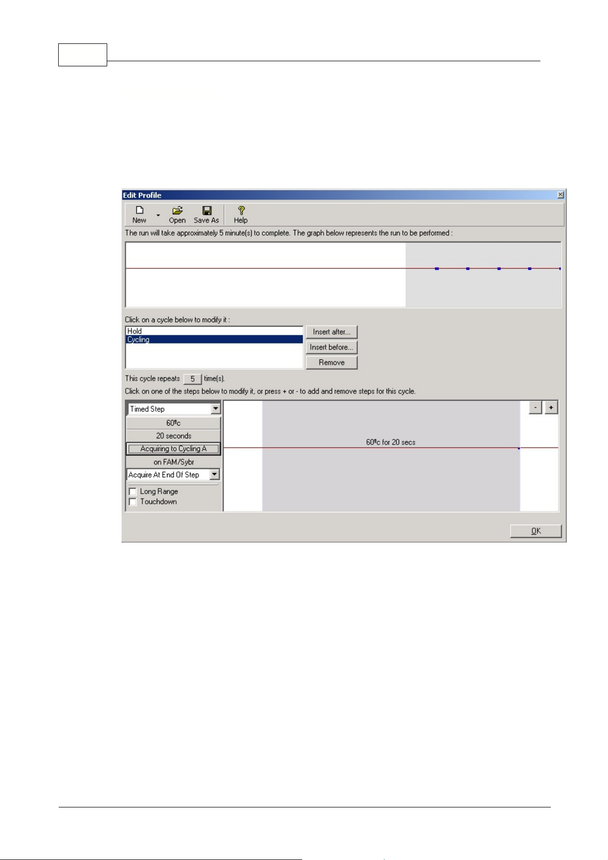
......................................................................................................................................................... 50Profile Editor

.................................................................................................................................................. 51Hold

.................................................................................................................................................. 51Optical Denature Cycling

IIContents

Rotor-Gene III

........................................................................................................................................... 51What is Optical Denature Cycling?

........................................................................................................................................... 53Configuration

........................................................................................................................................... 53Adding a New Optical Denature Cycling

........................................................................................................................................... 55Changing An Existing Step to Use Optical Denature

.................................................................................................................................................. 56Cycling

.................................................................................................................................................. 56Acquisition

.................................................................................................................................................. 57Melt

......................................................................................................................................................... 57Profile Progress

......................................................................................................................................................... 58Edit Samples

......................................................................................................................................................... 60Gain Calibration

.................................................................................................................................................. 60Auto-Calibration

.................................................................................................................................................. 62Manual Calibration

......................................................................................................................................................... 63Display Options

................................................................................................................................... 649 Gain Menu

................................................................................................................................... 6410 Window Menu

................................................................................................................................... 6411 Help Menu

......................................................................................................................................................... 65Send Support E-Mail

Part VI

General Functions Used Over Several Windows

................................................................................................................................... 651 Opening A Second Experiment

................................................................................................................................... 662 Spanner Icon

................................................................................................................................... 673 Scaling Options

................................................................................................................................... 674 Abbreviations

................................................................................................................................... 675 Auto-Scale

Part VII Quick Start Using The New

Experiment Wizard

................................................................................................................................... 681 Welcome Screen

................................................................................................................................... 692 Page 1

................................................................................................................................... 703 Page 2

................................................................................................................................... 714 Page 3

................................................................................................................................... 725 Page 4

Part VIII

Rotor-Gene Hardware Information

................................................................................................................................... 721 Filter Specifications

......................................................................................................................................................... 7232 Well and Dual-Channel Machines

......................................................................................................................................................... 73Multi-Channel Machines

Part IX Troubleshooting

................................................................................................................................... 741 Log Archives

................................................................................................................................... 742 Troubleshooting Experiment Files

......................................................................................................................................................... 75Initial Denature Step

......................................................................................................................................................... 75Cycling Profile

......................................................................................................................................................... 75Melt Curve Analysis

......................................................................................................................................................... 76Gain Settings

......................................................................................................................................................... 76General Setup Conditions

......................................................................................................................................................... 76Experiment Settings

................................................................................................................................... 773 Regional Settings In Windows 98

IVContents

Part X

Rotor-Gene 3000 Setup Instructions

Part XI Rotor-Gene 2000 Setup

Instructions

Part XII

Rotor-Gene 2000 IMPORTANT SETTINGS

Index

5 Rotor-Gene

Before running the Rotor-Gene you should pay attention to the following:

1) Always run the unit with 36 (32) or 72 tubes in the rotor. If you do not have this many samples load

empty tubes into the rotor. This ensures the thermal load in the chamber is identical for every run. If

0.1ml tubes are used it is sufficient to place empty tubes without lids into the rotor.

Do not use caps on the blank tubes. If caps are loaded on blank tubes and run multiple times

there is a risk that caps may come off the tube causing damage to the rotor.

72-well Locking Ring:

To ensure that tubes sit firmly in the 72 well rotor, a 72 well locking ring is

available. After loading the tubes, the rotor can simply be put over the rotor.

2) Ensure the software is not operating in the Virtual Machine Mode. Go to the

File menu

and select

Setup...

Check that the Virtual Machine box is not ticked.

Setup...

cannot be selected then it has been disabled and your distributor should have preset the

software.

3) Before running a program ensure the Rotor-Gene shows

READY

on the display. If

READY

is not

shown the machine will not set the Gains for the channels and no data will be collected.

The keyboard can be used to set the unit to a temperature and hold. In addition, the Rotor-Gene

keyboard display shows the lid status, either Open or Closed.

Pressing the

Next key

dvances the window forward to the next display and shows Lid Status then

Set Temperature.

Use the

and

Down

keys to change the set temperature, once set press

Start

The system then will go through a Start sequence that turns on the rotor, then the chamber fan and

then the heater.

The unit will heat or cool and hold the set temperature. This is useful if incubation at a particular

temperature is required before thermal cycling samples.

The keyboard can be used to set a manual temperature but is not used in regular operation.

The Rotor-Gene is setup using the following procedure:

1. Turn the desktop PC on and wait for Windows to boot up.

2. Turn on the Rotor-Gene on the left-hand side of the unit wait for the ready message to be displayed

on the LCD.

1 Introduction

1.1 Important: Read Before Running The Rotor-Gene

1.1.1 Rotor-Gene Keyboard (Rotor-Gene 2000 Only)

1.1.2 Rotor-Gene Startup

3. Double click on the Rotor-Gene icon.

4. The Rotor-Gene is now ready for use.

Note for Rotor-Gene 2000 users: If the Rotor-Gene is turned ON without having Rotor-Gene

software loaded and running on the PC, the instrument will emit a buzzing sound. By running

the Rotor-Gene software the buzzing will stop.

1.1.3 Software Version

Software development for the Rotor-Gene system is ongoing. To check on your version number click

Help

then

About Rotor-Gene...

The latest software version is available for download at our web

site.

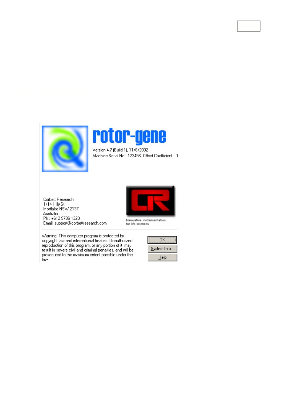
This screen displays general information about the software, and specifically includes the version of

the software, serial number of the machine, as well as the date it was last updated.

6Introduction

7 Rotor-Gene

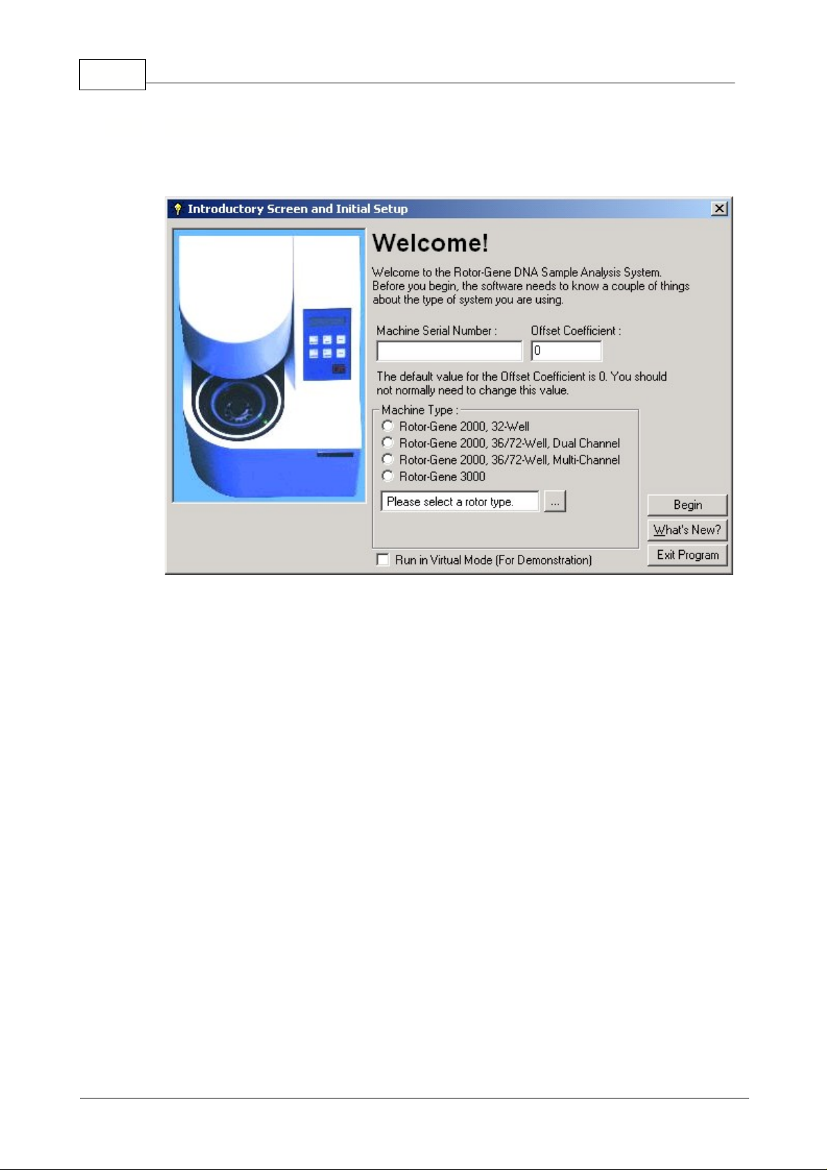
This screen appears when a new version of the Rotor-Gene software has been installed and the

Rotor-Gene icon is double clicked for the first time after the installation.

Machine Serial Number:

Type in the serial number (six digits), which is located at the back of the

Rotor-Gene.

Offset Coefficient:

Type in the Offset coefficient, which can be found next to the serial number of the

machine. If no number can be found, the value 0 should be entered.

Machine Type:

Chose your type of machine.

1.1.4 Welcome Screen

8Introduction

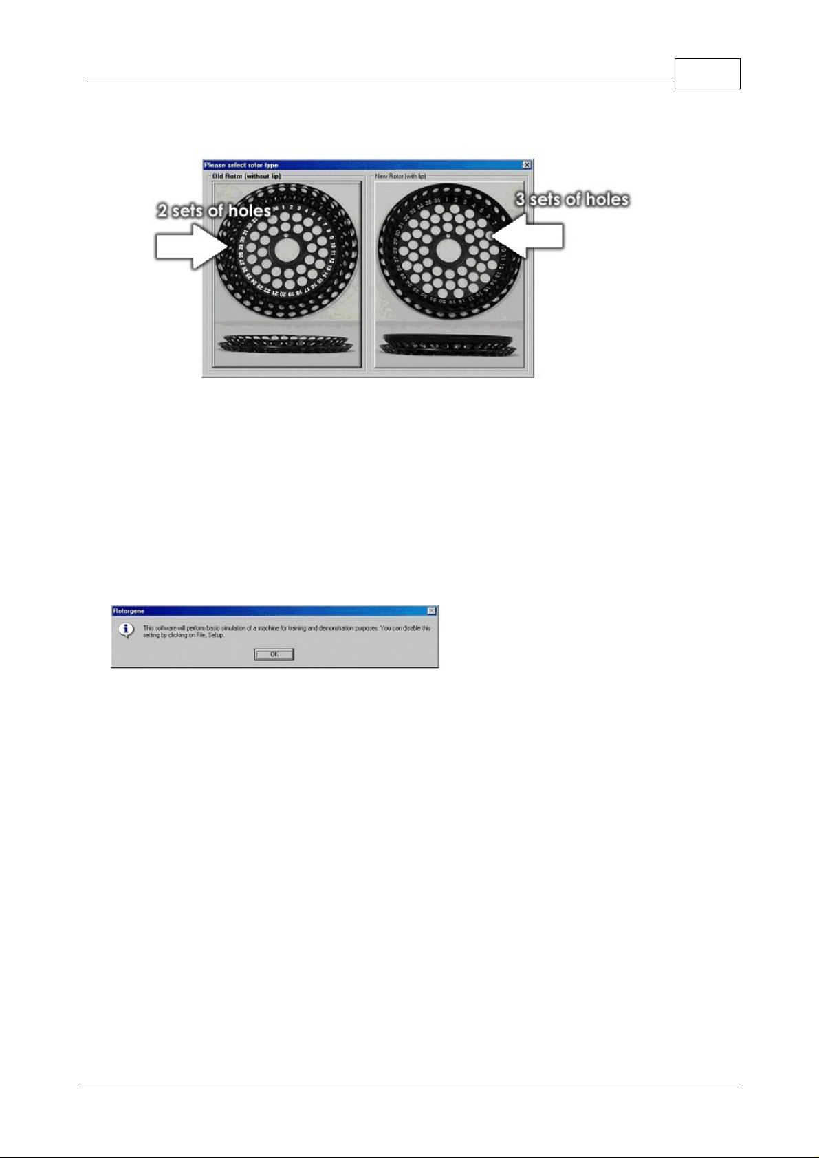
Choose type of 36 well Rotor:

Run in Virtual Mode

(for demonstration): Ticking the box allows installing the Rotor-Gene software

on a computer without Rotor-Gene attached. The software is fully functional and can even simulate

runs.

NOTE: If this box is ticked with a Rotor-Gene connected to your computer, a message will

appear before you start your run: "you about to run in virtual mode". To be able to perform a

"real" run, the setup (see setup) has to be changed.

Begin:

When all parameters are set, press Begin. A window will come up initializing machine. Wait

until the machine is initialized, which might take a few seconds. If virtual mode was chosen the

following screen appears:

If the box stays unticked the machine is initialized and opens up the Rotor-Gene software

automatically.

What's new:

This topic explains the new features in this version of Rotor-Gene and answers

commonly asked questions about the location of existing features that have been moved. These

features incorporate design changes and requests by users.

Exit Program:

Exits program.

9 Rotor-Gene

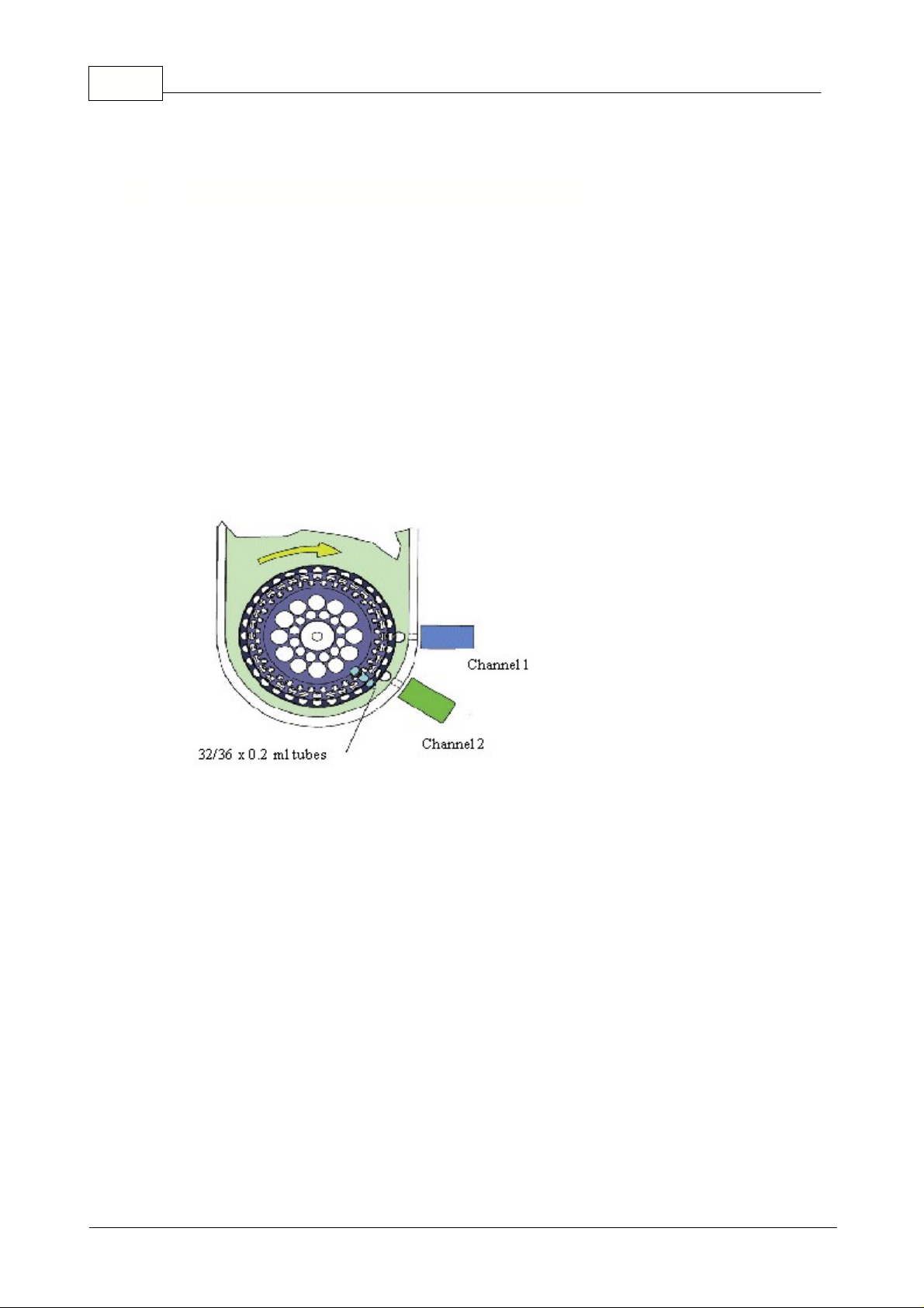
The Rotor-Gene is a real-time thermal cycling system used for DNA amplification and hybridization.

The unit holds 36 x 0.2ml standard micro-fuge tubes (32 x 0.2), which are loaded into a 36-position

rotor (32). With a Dual-Channel machine, a 72-well rotor is also supplied that can run special strip

tubes that are 0.1ml in strips of four. During the run the rotor spins at approximately 500 rpm as the

tubes are thermally cycled in a low-mass air oven.

NOTE: Always run a full rotor of tubes, for both the 72-well and 36-well rotors. If the number

of samples is small fill the remaining positions with empty tubes. This ensures the thermal

load of plastic tubes is the same from run to run.

There are two detection modules in the Rotor-Gene, Channel (1) is setup to detect 510nm and

Channel (2) is setup to detect 555nm. This allows for multiplexed samples to be run.

As the sample tubes spin past the detector modules, a high powered LED strobes the sample and a

photomultiplier (PMP) collects the fluorescent energy. See the figure below.

This data is sent to a Desktop PC that averages the energy of each sample over a number of

revolutions. This data is then displayed in real-time on the screen as fluorescence versus cycle

number or temperature plot.

2 Rotor-Gene Description

2.1 32-Well and Dual-Channel Rotor-Gene

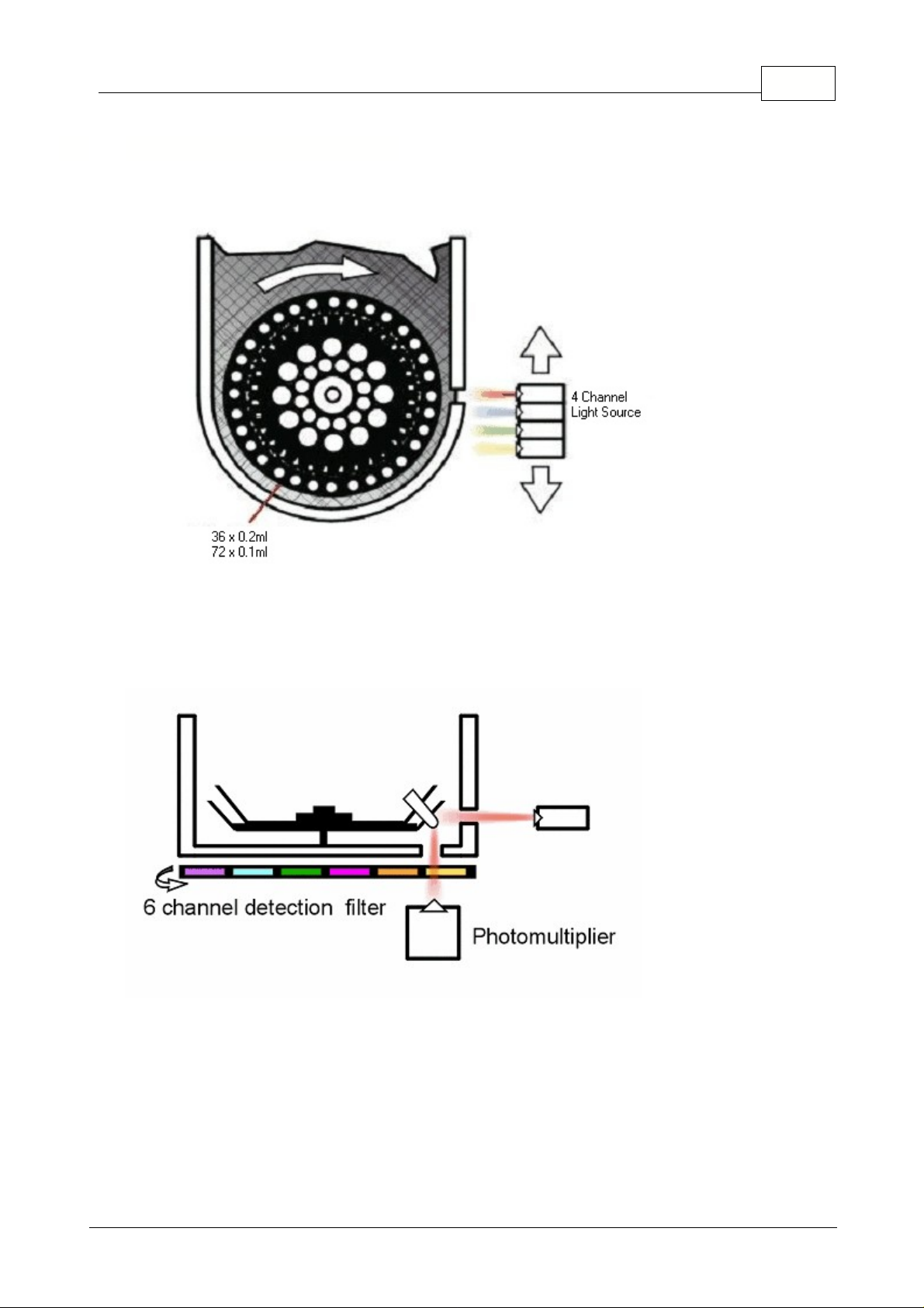
2.2 Multi-Channel Rotor-Gene

The principal of the Multi-Channel Rotor-Gene is very similar to the 32-well and the Dual-Channel

Rotor-Gene. However, the Multi-Channel has one LED with four excitation filters.

From the side view of the heating cooling chamber we see the LED source irradiating the tube from the

side wall and the photomultiplier detecting the energy from the base of the chamber. The detection

filter wheel has six different filters, four are band-pass that are used in four Channel multiplex runs, the

other two are high pass filters used with other non-standard fluorophores.

10Rotor-Gene Description

11 Rotor-Gene

Opening and closing 0.2 tubes several times before running might loosen the closing mechanism of

tubes. The 0.2 tubes run on the 36-well rotor on the Rotor-Gene should only be closed once before

running, otherwise it might result in popping of tubes.

Also make sure that the 0.2ml tubes are

closed properly by firmly pressing down the lid of the tube.

If popping is experienced or wants to

be avoided, a locking ring can be used on the Rotor-Gene.

The Locking Ring is designed to use

for flat top 0.2 ml tubes only.

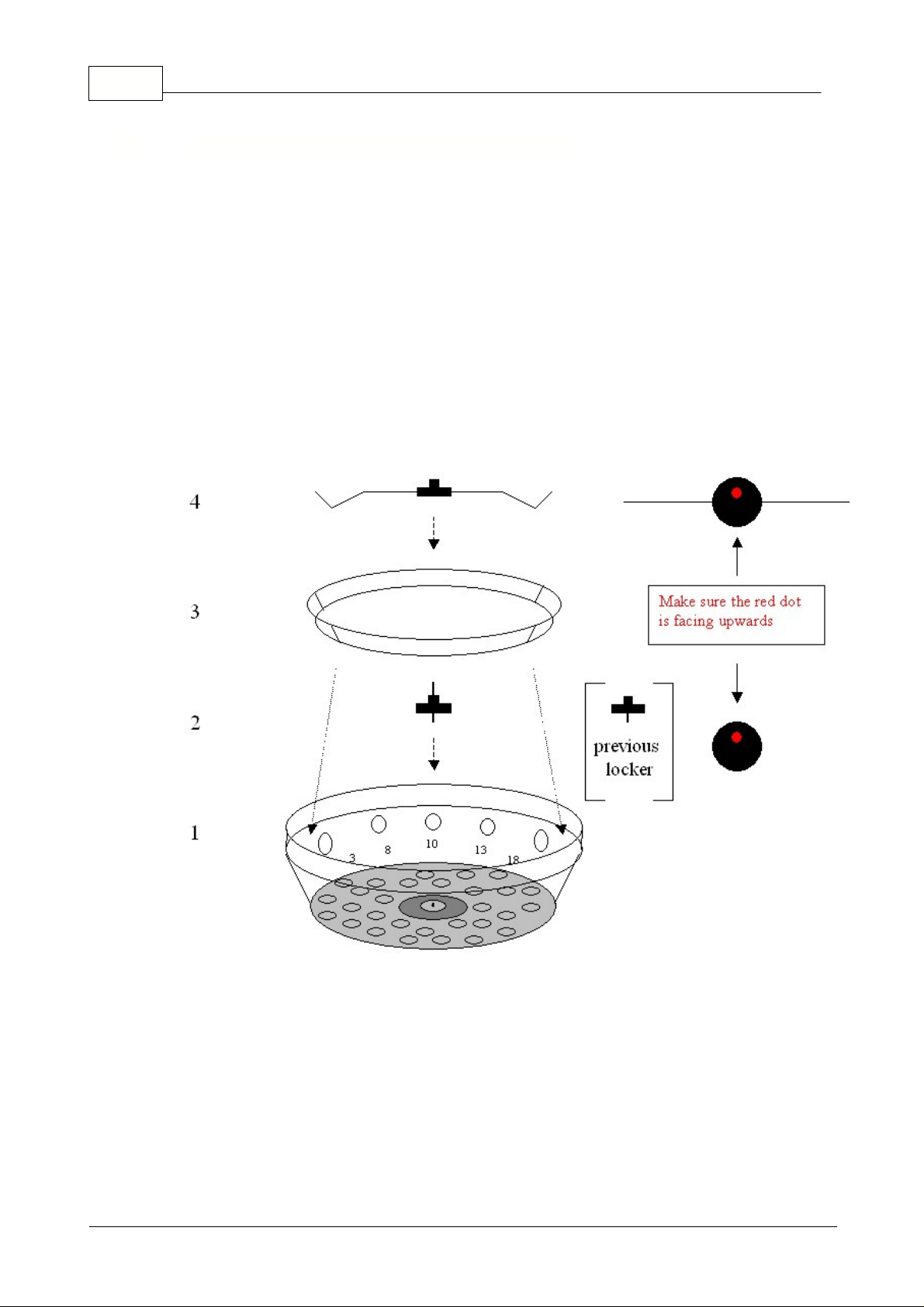
The below graph shows schematically how the locking ring has to be used:

1) Shows the schematic representation of the 36-well rotor.

2) Screw down the screw with threads on both sides. Make sure the nipple and the red dot faces the

top.

3) Simply place the locking ring over the top of the tubes.

4) Screw down the locking ring holder (4) over the screw with threads on both ends (2) until the

locking ring (3) is fixed.

2.3 Locking Ring (For 36 Well Rotor Only)

3 Two Different Rotor Systems (Tubes)

It is recommend that you use flat cap, 0.2ml tubes from Axygen

, supplied by Corbett Research.

If using your own tubes, be aware of the following:

1. The tube cap must fit down tightly otherwise there is a risk that the cap may 'pop' open during

thermal cycling. This has been observed with some domed capped 0.2ml tubes. If necessary the

locking ring could be used to secure the tubes.

2. Be sure that the tubes fit into the rotor firmly. Tubes that are excessively loose may vibrate during a

run and interfere with the data acquisition and give poor results.

3. In addition, ensure that the tubes are not too large. If the diameter of the tube is too large it will not fit

down far enough into the rotor. Samples will not be optically aligned over the detection system and may

cause a reduction in fluorescent signal acquired and sensitivity.

4. Do not use tubes from different manufacturers within the same run. This may result in

inconsistencies.

5. Locking Ring can only be used with

flat top

tubes.

Corbett Research manufactures the 72-well tubes and caps in strips of four especially for the Rotor-

Gene.

It is not advised to autoclave the 72-well tubes and strip caps as they may distort.

The tubes can become visibly deformed and are no longer straight but bent slightly. When running

tubes that have been autoclaved it has been noted that the caps may detach from the tube.

This has the effect of the loose caps being circulated around the chamber causing damage to the

insulation material. It is also advisable to exchange the empty 72-well tubes after at least ten runs.

Caps might start popping.

Do not use caps on the blank tubes. If caps are loaded on blank tubes and run multiple times

there is a risk that caps may come off the tube causing damage to the rotor.

The Rotor-Gene 2000 and the Desktop PC should be connected with the special "Y" mains cable

supplied. This special cable minimizes the connection length between the two devices.

NOTE FOR Rotor-Gene 2000 Users: If you do not set up the mains connection as described

you may see spikes in the collected data due to mains noise.

3.1 Rotor 36 Well System

12Two Different Rotor Systems (Tubes)

3.2 Rotor 72 Well System

4 Installation and Maintenance

4.1 Installation (Rotor-Gene 2000)

13 Rotor-Gene

No special installation steps are required for the Rotor-Gene 3000. The Rotor-Gene 3000 requires

only a standard serial cable to be connected to a communications port on the back of the Laptop or

Desktop computer.

The only maintenance the user may have to perform is keeping the lenses relatively clean and free

from dust that may build up over time.

It is recommended that when the Rotor-Gene is not in use, the lid is in the closed position to minimize

dust falling into the heater chamber.

Looking down into the heating chamber you will notice one (36/72-Well, Multi-Channel) or two (36/72-

Well, Dual-Channel) round lenses, which are the detector objectives for the different Channels. Should

those lenses be covered with dust or any other debris you should clean them using a cotton bud and

ethyl alcohol.

On the side-wall of the heater chamber there are also one (36/72-Well, Multi-Channel) or two (36/72-

Well, Dual-Channel) round lenses for the high power diode emitter. These lenses are not likely to build

up dust, however, if you place tubes into the rotor that are dirty or wet you are likely to spin those

particles around the inner wall of the heater chamber and possibly produce a build up on these lenses.

If these lenses need to be cleaned, the rotor can be removed by unscrewing the black lock-down in the

center and removing the rotor. These lenses can be cleaned with a cotton bud and ethyl alcohol.

The following chapter will help to familiarize you with elements in the Rotor-Gene user interface.

The Rotor-Gene workspace is the backdrop of the main window. This is the area in which you can

open up graphs of raw data, temperature and analysis results. If you have several windows currently

open, you can organize them by clicking the

Arrange button

on the toolbar. There are several

additional options available, which you can access by clicking on the

Down Arrow

, which appears

next to the button.

These buttons are shortcuts to frequently used operations. To see what their function is, hover your

mouse over them and a brief explanation will appear. These commands can also be accessed via their

corresponding menu items with the same name.

4.2 Installation (Rotor-Gene 3000)

4.3 Maintenance

5 Functional Overview

5.1 Workspace

5.2 Toolbar Workspace

5.3 View Raw Channels

Click on these buttons to view different channels in the experiment.

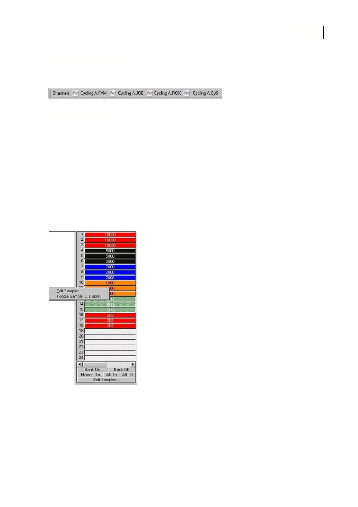
Use this control to hide or show different samples. Semi-greyed samples are deselected. The

Scroll

Bar

is used to display the next group of samples. You can toggle samples individually by clicking on

them, or you can hide/show all currently visible (on the current 'bank') by clicking on

Bank on/ Bank

off

. To select a range of samples, click on the first sample and drag your mouse to the end sample.

When you release the mouse button, the selected samples will either be toggled on or off. Clicking

Named On

will only show those samples you have given a name to; a quick way to show only relevant

samples. Clicking

All On /All Off

will show all/ none 36 or 72 samples. Pressing the

Edit Samples…

button opens the samples window.

Toggle samples ID display:

If a 72-well rotor is used the samples are shown from A1 to A8, B1 to

B8, etc. Using the toggle samples ID display button lets the user switch to a numerical order of

samples (1 to 72).

The sample toggler:

5.4 Toggle Samples

14Functional Overview

15 Rotor-Gene

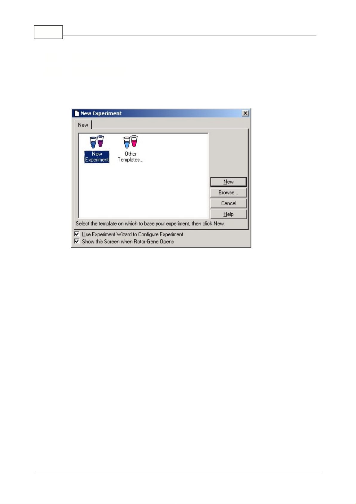
This screen presents you with a selection of available experiment templates. In a laboratory

environment, you can set up standard templates by placing them in the Rotor-Gene template directory

(usually C:\Program Files\Rotor-Gene\Templates). These templates will then appear in this window.

New Experiment:

Double-clicking this icon will create a new experiment based on the last experiment

run. To always begin with a blank experiment, choose File, Save As and save a template in the Rotor-

Gene template directory as "Blank Template.ret". Then, double-click this icon instead of New

Experiment when starting a new run.

New...:

Opens the template selection window to create a new experiment.

Browse...:

Pressing Browse... opens a window in which you can select the template you would like to

use for the next run. This option is also available under Other Templates.

Other Templates...:

This icon has the same effect as clicking the Browse... button, and displays an

open dialogue to load custom experiment templates.

Cancel:

Closes this window.

Help:

Opens on-line help.

Use Experiment Wizard to Configure Experiment:

Upon selecting a template, the New Experiment

Wizard will be displayed. Unticking the Use Experiment Wizard option can disable the wizard.

Show this screen when Rotor-Gene opens:

Untick the box if you don't want to see this window

coming up before using the Wizard.

5.5 File Menu

5.5.1 New Experiment

5.5.2 Opening and Saving

Open...:

Opens a previously saved Rotor-Gene Experiment (REX file) or Rotor-Gene Experiment

Archive (REA file).

Open Recent...:

Displays the last four files you have opened or saved.

Save:

Saves the experiment, prompting you for a filename if this is the first time the experiment has

been run. You have the option of saving the experiment as a template, meaning that you can base

future experiments on it. You can also save in the Rotor-Gene Experiment Archive (REA) format that

compresses the experiment. This is ideal for emailing, as it does not need to be compressed before

sending.

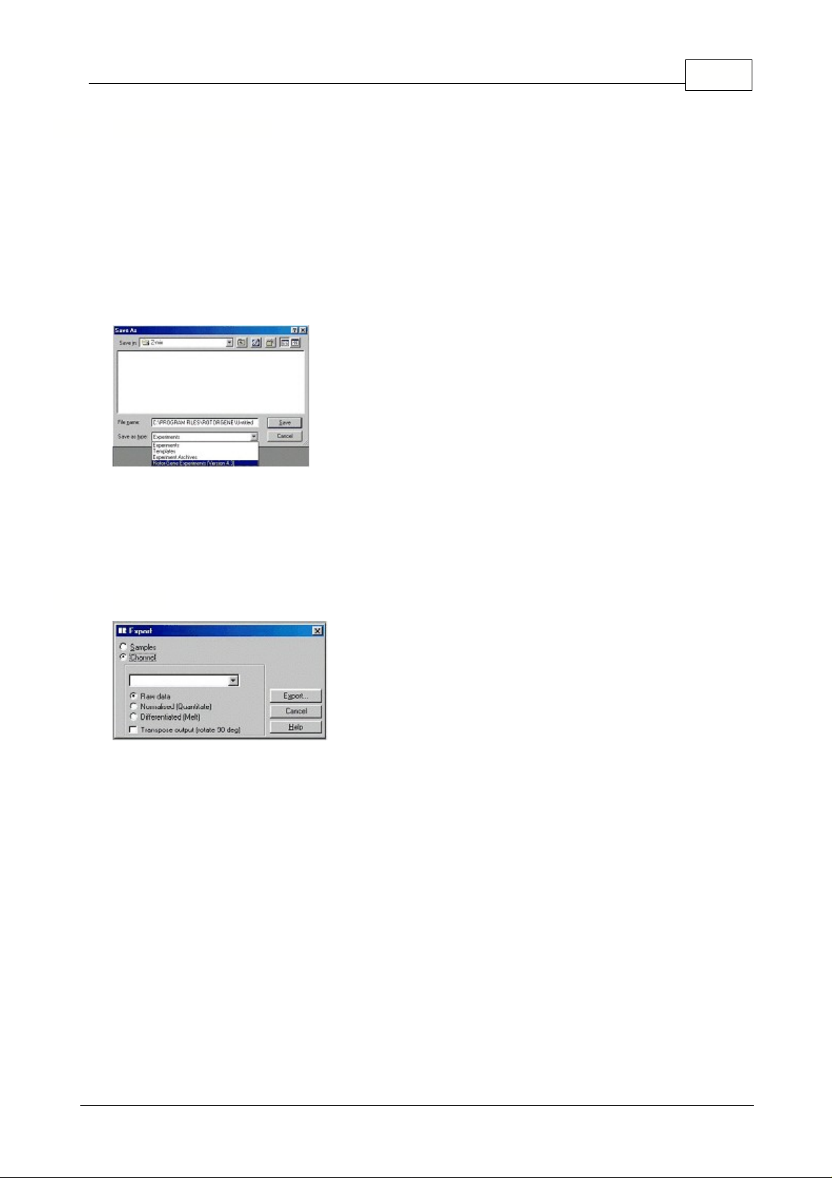
Save As...:

Saves the experiment, always prompting you for a filename. It also lets you choose what

type of file you want to save the document as.

A file can be saved as an experiment, a template, an experiment archive or an experiment in a previous

RG software version (4.3).

Opens the Export window where you can export channel and sample data to a format readable by

other software. You can export Rotor-Gene data to third party software such as spreadsheet and

statistical applications. This screen allows you to export channel information and the sample list.

Export Samples:

The experiment's sample list will be saved in a format, which can be opened by

popular spreadsheet applications. Once you have saved the samples, drag the export file into your

spreadsheet.

Export Channels:

You can export both raw data obtained from the machine and the data used to

perform analysis after normalization and other operations have been performed. Select the channel to

export, and the type of data you wish to export, then click Export. The resultant file can be opened by

dragging it into the target application.

16Functional Overview

5.5.3 Export

17 Rotor-Gene

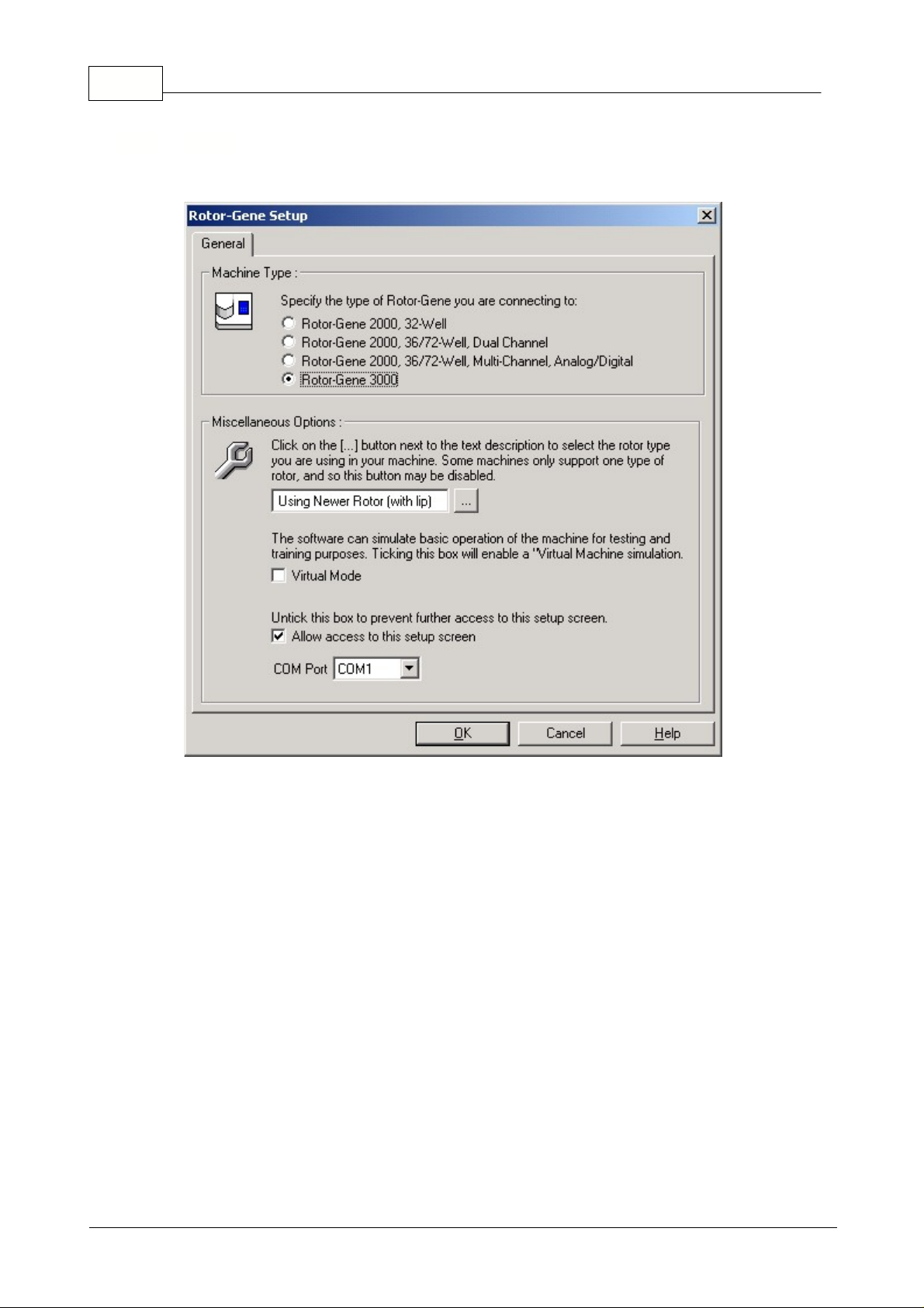
Choosing File, Setup... opens the Rotor-Gene setup window.

Machine Type:

Select the machine you are operating from the option buttons available.

Virtual Machine:

This option enables you to operate the software even when a machine is not

attached for demonstration purposes.

Allow access to this screen:

Untick this box, once the machine has been correctly selected to

prevent users from altering this setting. If you need to have access to this screen again, contact your

distributor.

5.5.4 Setup

5.6 Analysis Menu

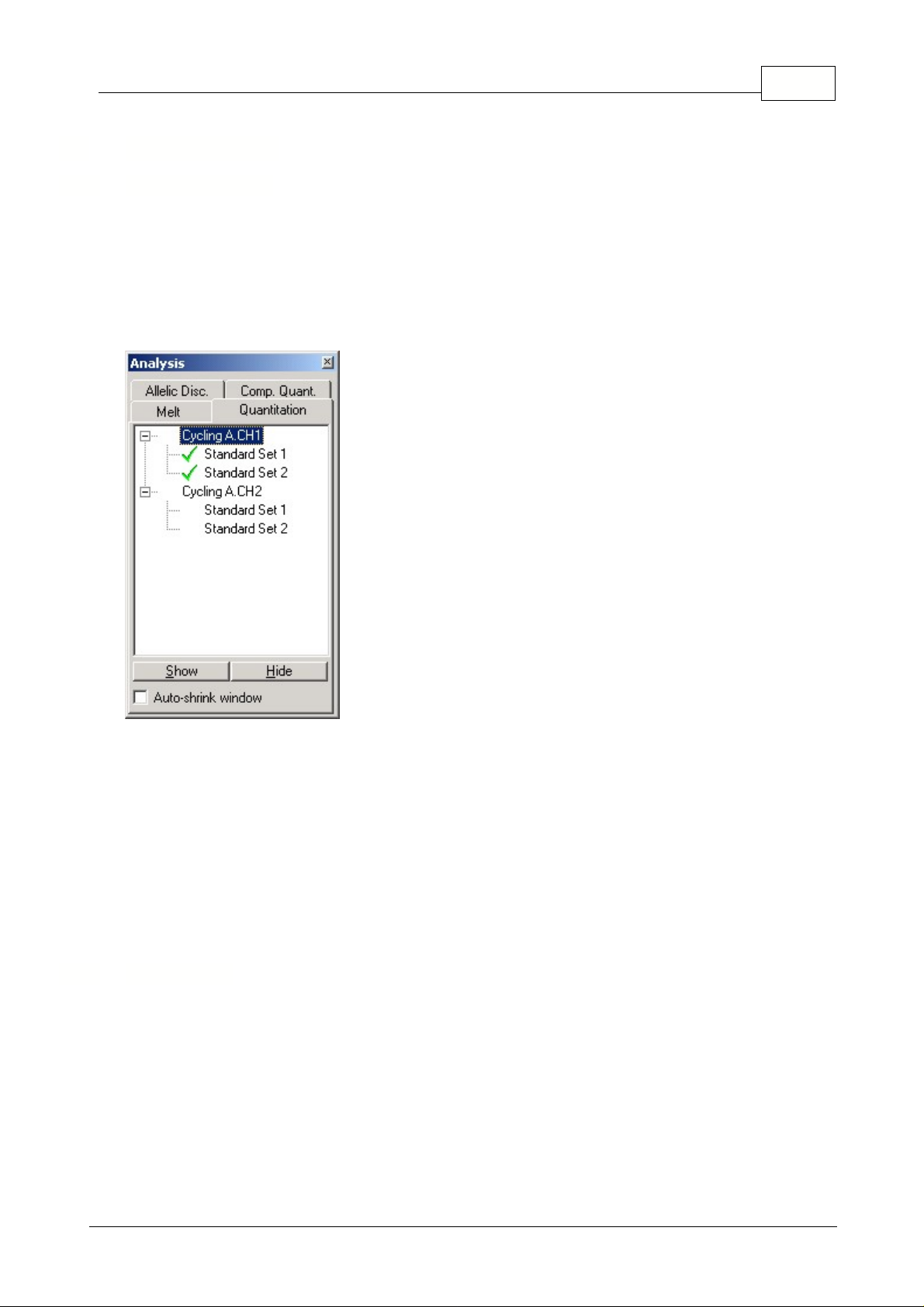
This toolbar enables you to create new analyses and displays existing ones. The tabs at the top of the

bar enable you to select a method of analysis to perform. Once you have done this, a list of the

channels which can be analyzed using this method will be listed below. Those that have already been

analyzed will have a green tick next to them, such as the first two channels shown in the screen shot.

This means that threshold and normalization settings have been remembered for this analysis. To

analyze a channel, or view an existing channel, simply double-click on the channel to view. The

specific analysis window will then appear.

Auto-shrink Window:

Ticking the box shrinks the window when it is not used. Moving the cursor over

the window enlarges the window again.

Organizing Your Workspace:

Each time you double-click on a new analysis, its windows will be

arranged to fit in with those already on the screen. With many windows, this can be difficult to use.

Simply close the windows you do not require, then click

Arrange

on the toolbar. The windows will

automatically be rearranged according to the

Smart Tiling

method. You can select another method of

arrangement by clicking the

down arrow

next to the toolbar button.

Clicking the right mouse button over the analysis window also allows to

Show, Hide

Remove

Analysis

Double click quantitation or press

Show

to open the channel of interest. Three windows will be opened

automatically, the main screen, the standard curve and the results. Going from left to right, the

following buttons are displayed in the main window:

5.6.1 Analysis Toolbar

18Functional Overview

5.6.2 Quantitation

19 Rotor-Gene

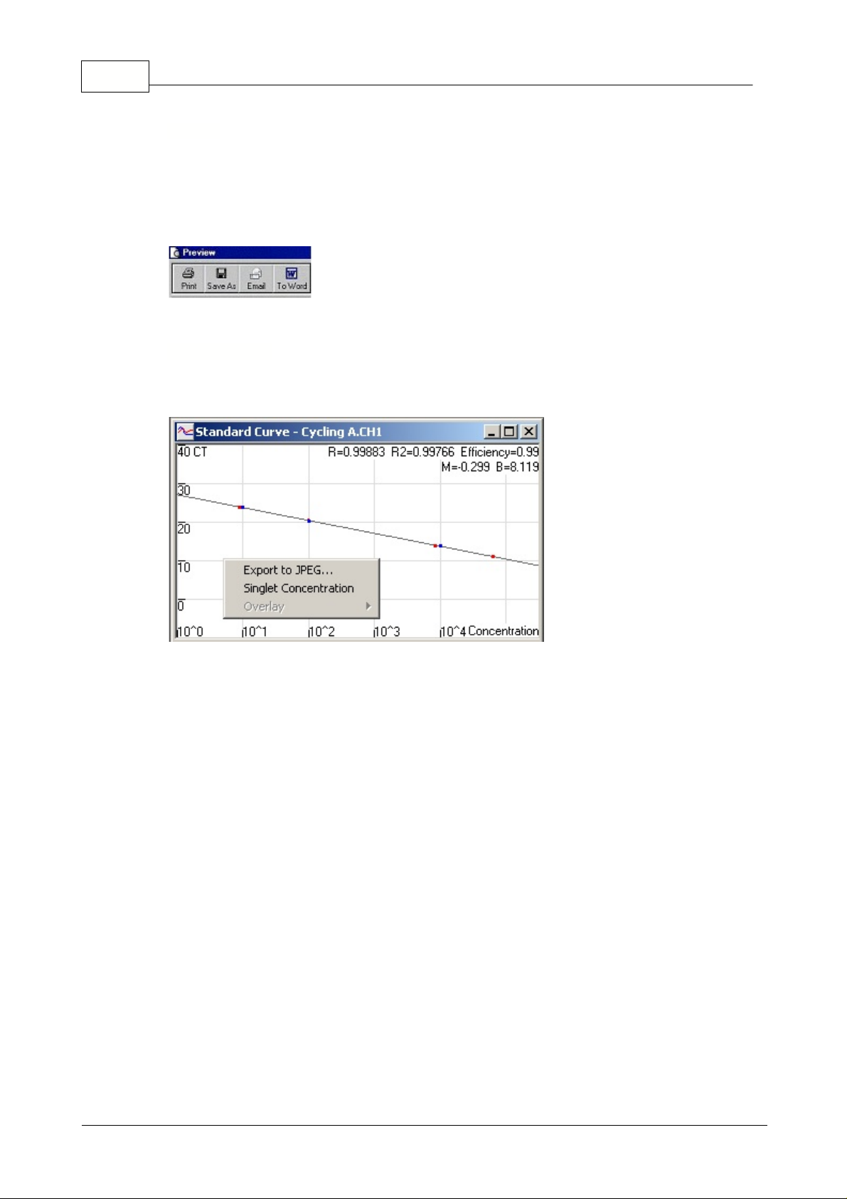
Reports:

Opens the Quantitation Report selection window where you can choose a report to preview

of the currently selected Quantitation analysis. There are three different options, Standard Report, Full

Report and Concise Report.

Using the buttons on the top, the reports can be

printed, saved, emailed

exported to Word

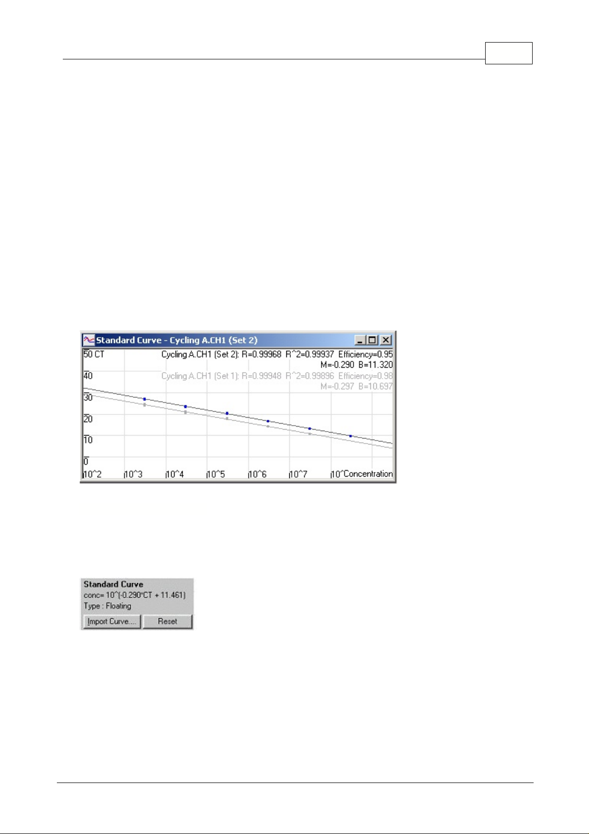
Std. Curve:

This button opens the standard curve graph. By default, this window is opened when an

analysis is opened. If you close the window, it can be re-opened by using this command.

On the standard curve the values are recalculated dynamically as the threshold level is varied, by

clicking and dragging.

Blue dots

on the curve show the samples that have been defined as standards and

red dots

show

the unknown sample data points.

NOTE: If redefining standards to recalculate the standard curve, toggling the standard colors

ON or OFF will remove it from standard curve calculation.

Efficiency:

The Reaction Efficiency of the experiment. This value is discussed in more detail in

Slope,

Amplification, Reaction Efficiency

R^2-value

(correlation coefficient):

The R^2 value, or R

value (as displayed with the superscript),

is the percentage of the data which is consistent with the statistical hypothesis. In the Quantitation

context, this is the percentage of the data which matches the hypothesis that the given standards form

a standard curve. If the R

value is low, then the given standards cannot be easily fit onto a line of best

fit. This means that the results obtained (ie. the calculated concentrations) may not be reliable. A good

R2-value is around 0.99.

NB: It is still possible to achieve a high R^2 value with a poor standard curve, if not enough

Reports

Standard Curve

20Functional Overview

standards have been run. The R^2 value will improve as the number of standards decreases.

R-value

(square root of correlation coefficient):

The R-value of the calculation is the square root

of the R^2 value. Unless you have a specific statistical application, the R2 value is more useful in

determining correlation.

According to the formula

y = mx + b

the slope (

) and the intercept (

) of a standard curve are

automatically calculated and shown in the top right corner of the standard curve window.

Export to JEPG...:

With the pointer on the standard curve, click on the right button to show the option

to export as a JEPG.

Singlet Concentration:

This function is used when no replicates on a standard have been run or

defined. With the function enabled the standard curve shows a line between the Given concentration

and the Calculated concentration for the standard series. The threshold is then optimized, by moving

the level to minimize the distance between each Given and Calculated standard concentration.

Overlay:

When multiple quantitation runs have been performed in the same experiment, it is possible

to overlay the standard curves in the same window. This is useful for graphically viewing the difference

between different thresholds on the statistical results. Below is a screenshot of this feature:

"conc=...*CT + ..."

represents the equation used to relate CT values and concentrations. Type can be

either floating or fixed. If floating, an optimal standard curve equation is calculated as you move the

threshold. If Fixed, the equation does not change because it has been imported from another

experiment.

Note: The Rotor-Gene standard curve formula is displayed in a different format to

competitors' standard curves. Competitors express their curve in terms of concentrations

instead of CT values, which does not affect results, but does affect the display of the M

(gradient) and B (offset) values. Please read the section

Why Are Rotor-Gene Standard

Curves Different?

for more information.

Standard Curve Calculation

21 Rotor-Gene

Importing a standard curve allows you to perform estimates of concentrations when a standard curve

is not available in an experiment and you are certain that the reaction efficiency has not varied between

the two runs. You can import curves from another channel, or from another experiment by clicking on

Import Curve.

You can choose to

Adjust

the standard curve, or not to adjust. Adjusting means modifying the offset

(b) in the standard curve to be consistent with the current experiment. Whether you should adjust the

standard curve or not depends on the chemistry application.

A reference should be defined in the target experiment to adjust the curve to match the target

experiment. You can define a reference by setting a sample's type to Standard, and entering a

concentration value in the Sample Editor. Multiple copies of the same reference can be entered to

improve accuracy of the method. Note that you cannot define more than 1 reference concentration. For

example, it is possible to have 3 replicate references of 1000 copies, but not to have one reference of

1000 copies, and another with 100 copies in the same experiment.

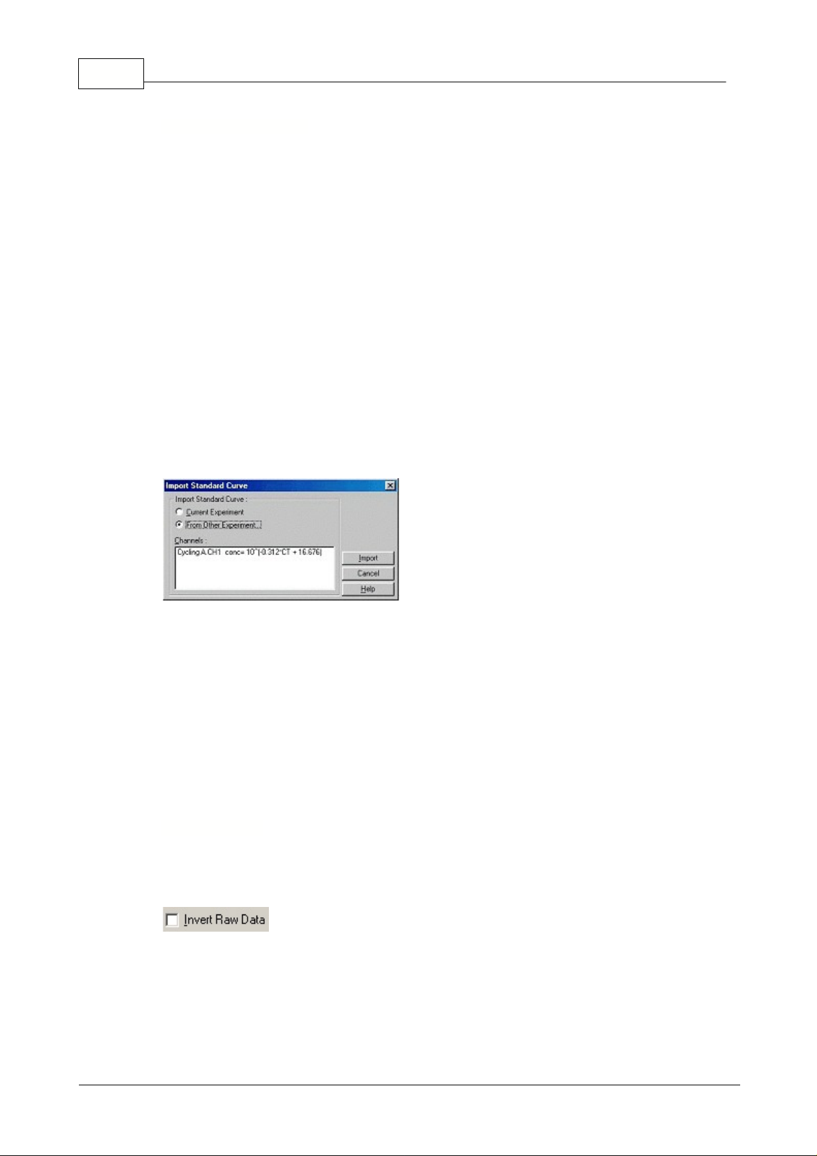
Once the curve has been imported, the standard curve type will be changed to Fixed. Click

Reset

set the curve type back to Floating.

Below is a screenshot of the Import Standard Curve screen:

Using this screen, you can import the standard curve from another channel you have analyzed in the

current experiment, or you can load a standard curve from another experiment.

Current Experiment:

When this option button is selected, quantitation analyses on other channels

will be listed with their corresponding standard curves.

From Other Experiment:

Selecting this option button will bring up an Open Dialog in which you can

select an experiment to open. If any quantitation analysis has been performed for the experiment, you

will see standard curves listed for each channel analyzed.

Channels List:

Lists the analyzed channels and their respective standard curve formulas.

Some chemistries produce a fluorescent readout that decreases exponentially instead of increasing. It

is still possible to analyse these using Quantitation, but the "Invert Raw Data" checkbox should be

ticked.

For all other quantitation analysis, this option must remain unticked.

Import Standard Curve

Invert Raw Data

NB: Techniques such as Quenched FRET

or the use of Bodipy

which use decreasing

signals to quantitate may have less accurate results than those that increase. Such

techniques have not been widely verified yet in the scientific community.

Calculation of CT

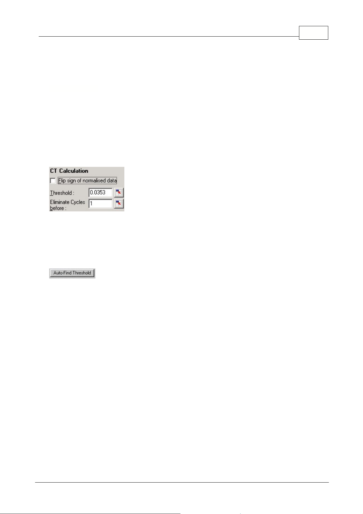
Ct-Calculation:

The Ct value is the value where the threshold line crosses the amplification curve. By

setting a threshold line and calculating the intersection with each of the sample curves, the Ct values

for each sample are established.

Threshold:

(Manual Set): To set the threshold click on the icon (grid with red arrow) then click and

hold on the graph and drag a threshold line to the desired level, or enter a log value. Alternatively the

Auto-Find Threshold function can be used to automatically determine the best level. When setting a

threshold manually, it should be set in the exponential phase of the experiment, significantly above the

background level to avoid noise.

Auto Find Threshold:

The automatic threshold function will scan the darkened region of the graph to

find a threshold setting which delivers optimal estimates of given concentrations. You can change the

region to be modified by entering new upper and lower bounds in the text boxes. For most quantitation

analyses, the default region is suitable. Based on the standards that have been defined the function

then scans the range of threshold levels to obtain the best fit of the standard curve through the

samples that have been defined as standards, (i.e. maximizes the R value to approach 1.0).

Eliminate Cycles before:

To set click on the icon (grid with red arrow) then click and hold on the

graph and drag the threshold line to the right. This eliminates the threshold line for low cycle numbers.

Note: This is useful when there is noise on the signal during the initial cycles.

22Functional Overview

23 Rotor-Gene

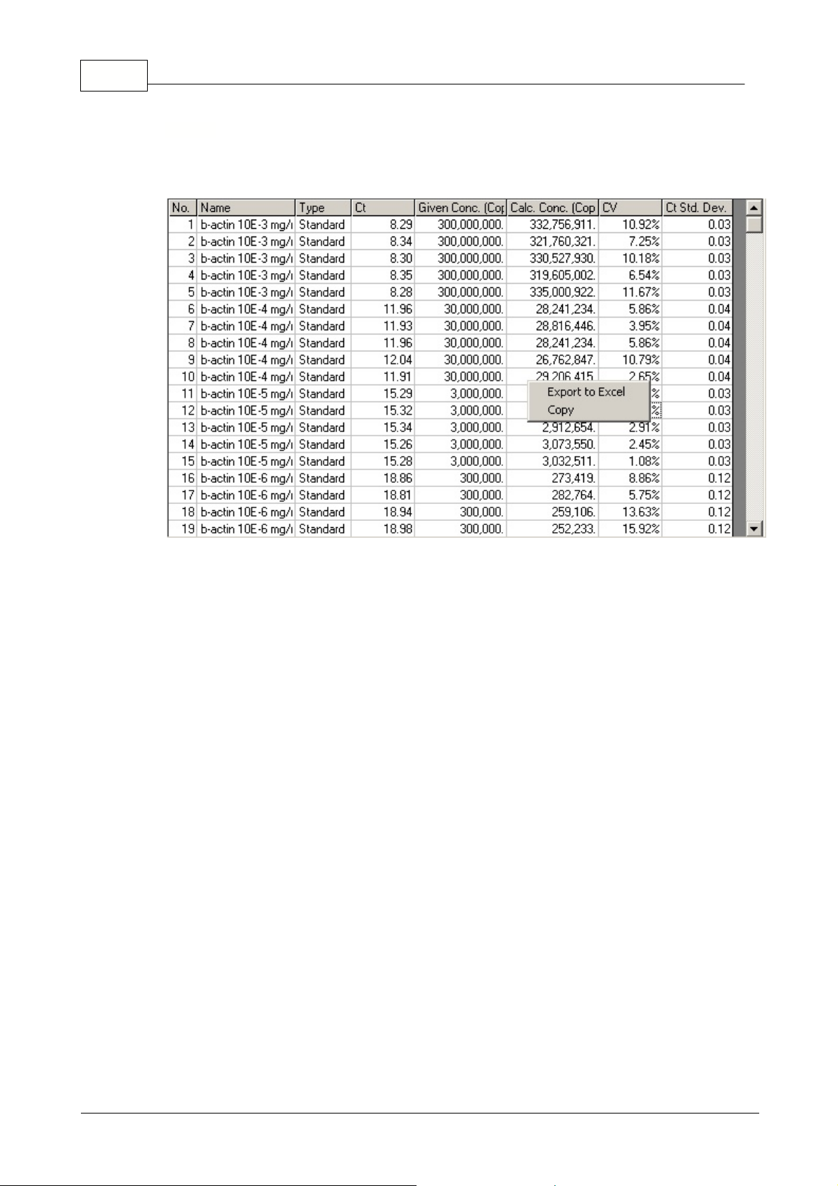
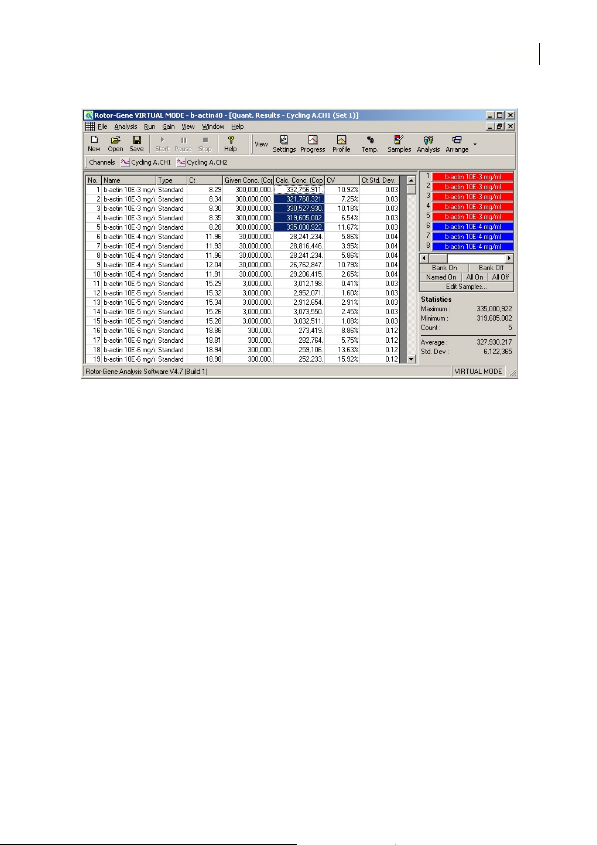
Opens the quantitation results grid. By default, this window is opened when you open an analysis. If

you close it, it can be re-opened by using this command.

The results obtained from the experiment are summarized in a table. Clicking the right mouse button,

and selecting

Export to Excel

will export the table to Excel. There is no need to open the Excel

program, as this will be done automatically.If you would like to copy the data into an existing

spreadsheet, choose the

Copy

option instead, then open your spreadsheet, then select paste.

To make calculations easier, a feature called

AutoStat

is introduced which automatically calculates

the Average, Standard deviation, Minimum and Maximum values of samples of interest. Simply move

the mouse over the area of interest and the values are given in a small table displayed below the

sample list on the right-hand side of the screen.

Results

24Functional Overview

In this screenshot, samples 1 to 5 are analysed:

This option is ticked by default and is used to determine the average background of each individual

sample just before amplification commences. Standard Normalization simply takes the first five cycles

and uses this as an indicator for the 'background' level of each sample. All data points for the sample

are then divided by this value to normalize the data. This process is then repeated for all samples. This

can be inaccurate as for some samples the background level over the first five cycles may not be

indicative of the background level just prior to amplification. Dynamic Tube Normalization uses the

second derivative of each sample trace to determine a starting point for each sample. The background

level is then averaged from cycle 1 up to this starting cycle number for each sample.

This method

gives the most precise quantitation results.

Alternatively with some data sets it may be necessary

to disable the dynamic tube normalization. If this is the case the average background for each of the

samples is only calculated over the first 5 cycles. If the background is not constant over the cycles

before amplification it will result in less precise data.

The background fluorescence (Fl) of a sample should ideally remain constant before amplification.

However, sometimes the Fl-level can show an increase or decrease due to the effect of the chemistry

being run and produce a skewed noise level. The Noise Slope Correction option uses a line-of-best-fit

to determine the noise level instead of an average, and normalizes to that instead. Turning on this

option can tighten replicates if your sample baselines are noticeably sloped.

This function improves the data when raw data backgrounds are seen to slope upward or downward

before the amplification take off point (Ct). It is very helpful for experiments when for example the FAM

background is seen to creep upwards over the initial cycles.

Dynamic Tube Normalisation

Noise Slope Correction

25 Rotor-Gene

The first couple of cycles in a quantitation run are not usually representative of the rest of the

experiment. For this reason, you may get better results if you select to ignore the first few cycles. If the

first cycles look similar to cycles after them, you will gain better results by disabling this function, as

the normalization algorithm will have more data to work with. You can ignore up to ten cycles.

The quantitation setting in the quantitation screen allows excluding samples or NTCs, which have a

slight drift upwards, due to probe degradation or other effects. All samples with a change below the

NTC threshold will not be reported in the quantitation screen. The percentage is relative to the largest

maximum change found in any tube. For example, if you have one sample which began at a

background of 2Fl and went to 47Fl, then 45Fl represents 100%. An NTC threshold of 10% would

consider as noise any sample with a reaction less than 4.5Fl.

The slope (m) of a reaction (shown in the standard curve window), once slightly transformed, can be

used to determine the exponential amplification and efficiency of a reaction.

Calculate a gradient g = 1 / m. This gradient g is used in the following equations, and not the m value.

This is because the slope used in the Rotor-Gene software and in other applications is reported in a

different but equivalent manner. The reason for this is explained in the topic "Why are Rotor-Gene

Standard Curves different?".

The following calculations give some important results:

exponential amplification = 10

(-1/g)

orreaction efficiency = [10

(-1/g)

] – 1.

Optimal values for g, amplification and reaction efficiencies are

–3.322, 2 or 1, respectively. The efficiency of a reaction is reported in the quantitation report.

The slope is calculated of being the change in Ct divided by the change in log input (for example copy

number). A 100% efficient amplification means a doubling of amplification product in each cycle

resulting in a g value of -3.322, an amplification factor of 2 and a reaction efficiency of 1.

Given a g value of –3.322, the calculations are as follows:

Amplification value:

(-1/-3.322)

= 2,

Reaction efficiency:

[10

(-1/-3.322)

] – 1 = 1.

Here are two examples for two different slope values.

A g value of 3.8 means that the reaction has an amplification value of ~1.83 and a reaction efficiency

of 0.83 (or 83%).

There could be several reasons for this value. If the value needs to be improved, optimization steps like

Ignore First

Quant. Settings

Slope, Amplification, Reaction Efficiency

primer or probe concentrations, MgCl

- or Sybr-Green I concentrations could be improved.

A g value of 3 means that the reaction is more than 100% efficient. A reason for this could be an

unproportional digestion of probe compared to the amplicon produced. In addition, if the R-value is low,

then statistical error can cause an unexpected reaction efficiency.

Offset

Intercept:

In a formula describing the relation between two variables, the intercept is expressed with the letter "b"

(y = mx + b). The intercept is also sometimes referred to as the

Offset

The intercept used in the standard curve of the Rotor-Gene software is the maximum theoretical

number of copies that could have been detected at cycle number 1.

Example:

The below shown standard curve has the following values:

R = 0.99977

M = 0.268

B = 10.393

A dilution series has been performed starting with a copy number of 10

copies. Four dilutions have

been performed down to 10

copies.

The intercept in this example is B = 10.393. The doted blue line below represents a CT-value of 1 and

the red line is an extrapolation of the standard curve. The crossing point of those two lines gives the

maximal theoretical amount of copies which could have been detected. The calculation is as follows:

Calculation:

26Functional Overview

27 Rotor-Gene

The short answer is that the Rotor-Gene standard curves and the competitor standard curves display

exactly the same information, but in a different manner. If you are not satisfied with this explanation,

then this section is of interest to you.

Many competitors provide a standard curve as a linear function from concentrations to CT values. This

means, the standard curve formula they produce allows to you to find out the CT value for a sample if

you know its concentration. The Rotor-Gene contains a formula written the other way around. That is,

given a CT value, tell me the concentration. Of course, this is exactly what the Quantitation process is

all about -- finding out concentrations of samples given their CT values. This is the reason we chose

this method of representing the information. The different approaches of the Rotor-Gene and

competitors has, however, been the source of some confusion.

This is the relationship between the values:

"competitor m value" = 1 / "Rotor-Gene m value"

"competitor b value" = -"Rotor-Gene b value" * "competitor m value"

Here is the proof of the correlation between the Rotor-Gene and Competitor standard curves. It is a

basic rearrangement of two functions.

Let rm, rb be the Rotor-Gene gradient and offset.

Let cm, cb be the Competitor gradient and offset.

Let Concentration be the calculated concentration for a sample.

Let CT be the CT value for a sample.

Now,

Log(Concentration) = rm * CT + rb

(Rotor-Gene has a function from CTs to Concentrations)

and

CT = cm * Log(Concentration) + cb

(Competitors have a function from concentrations to CTs)

Then,

Log(Concentration) = rm * CT + rb

(rearranging)

(Log(concentration) - rb) / rm = CT

(Log(concentration) - rb) * 1 / rm = CT

Let f = 1 / rm

(Log(concentration) - rb) * q = ct

Log(concentration) * q - rb * q = ct

(refactoring)

let g = -rb * f

Then

CT = Log(Concentration) * f + g

Which is exactly the same as the competitor equation, by substituting

f == cm and g == cb.

Why Are Rotor-Gene Standard Curves Different?

28Functional Overview

Thus,

cm = 1 / rm and cb = -rb * cm

29 Rotor-Gene

This screen shows that taking the average background energy for each of the samples normalizes the

data which is then converted to a Log scale.

From this Log graph a threshold can be determined to calculate the Ct value for each of the samples.

The Ct value denotes the starting cycle for the amplification. This Ct value can be related directly to the

starting copy number of the sample.

Pressing

Linear Scale

on the bottom of the screen takes you directly from the

Log Scale

to the

Linear Scale

or the other way round.

The difference between the Linear and the Log Scale is only how the data is presented. The lower

values in the Log-Scale are "blown up" to make data readable easier. The Log Scale emphasizes the

normalized data approaching zero. The linear scale is the normalized RAW data, we see all samples

with the same starting background.

The log-scale is the LOG of the normalized data, we see the small increase at the take off point

expanded so we can accurately determine the Ct value. This could easily be checked by turning on the

pinpointer in both graphs and compare the numbers obtained for the fluorescence. It can be seen that

there is no difference between the actual data.

Note: This process can also be performed while the Rotor-Gene is running. This real-time

monitoring of quantitation data provides the user with the possibility to gain results as soon

as the curves show an exponential growth. Preliminary conclusions could be drawn already

and decisions made for the next run.

Main Window

5.6.3 Melt Curve Analysis

Melt Curve analysis

analyses the derivative of the raw data, after smoothing. You can use it to

perform genotyping, to find take-off points in reactions and numerous other applications. Peaks in the

curve are grouped into bin groups, and all peaks below the threshold are discarded. You then map

bins to genotypes through the Genotype, Edit Genotypes menu.

Typically after a cycling run has been finished a melt step can be added to visualize the melt

characteristics of the products. The sample temperature is increased at a linear rate and the

fluorescence of each sample is recorded.

Below is a typical melt curve analysis shown for a Sybr Green I amplification.

Flip sign of dF/dT:

Before defining peaks ensure the dF/dT sign is correct for the data set to give

positive peaks.

Defining Peaks:

In the Melt Curve Analysis screen peaks can be defined and reported using different

methods. One is to automatically call all the peaks for each sample. The other is to assign peaks to

bins, which is useful for genotyping samples.

Any peak that is within a range of +/-2°C of the bin center will be assigned to the bin. If there are two

peak bins close together then the peak will be assigned to the closest bin.

Bins are used to define the general area where you expect peaks to occur. The melt analysis software

clusters peaks into bin groups, based upon actual peak values in the curve.

30Functional Overview

Sidebar

31 Rotor-Gene

Note: The peak bins should not be used for estimating peak positions, use the Automatic

Peak Calling table instead for this purpose.

Peak Bins:

To define a peak bin click on the

New Bin

button, then click and hold on the graph to

define the center of the peak bin. To add another bin repeat the process or use the

Remove

button to

delete peak bins.

Threshold Level:

To set the threshold, click on the icon (grid with red arrow) then click and hold on

the graph and drag a threshold line to the desired level.

Temperature Threshold:

To set click on the icon (grid with red arrow) then click and hold on the

graph and drag the threshold line to the right. This eliminates the threshold line for the lower

temperatures.

Note: This is useful when there is noise on the signal at low temperatures.

Opens the Melt Report selection window where you can choose a report to preview. You can generate

a report based upon the currently selected channel, or you can generate a Multi-Channel genotyping

report.

Displays the result grid, showing peaks in samples.

Click on the genotyping toolbar and select the genotype definitions.

This screen lets you assign genotypes to the incidence of peaks in bins. The default genotype

configuration is shown in the screenshot, with heterozygous samples having two peaks, homozygous a

peak in the first and wild type samples in the second bin. Next to the name of each genotype is a field

for typing in an abbreviation. This is used when printing multi-channel genotyping reports so that all

results from multiple channels can be read easily across the screen.

For multiplex analysis, genotypes have to be setup in each channel. If for example a dual

channel FRET analysis is run, where a wild type, heterozygous and homozygous is expected

in each channel, the above setup has to be performed for each channel. The results will than

be given in a multiplex report.

Reports

Results

Genotyping

5.6.4 Allelic Discrimination

For Allelic Discrimination, it is not sufficient to double-click on the channel you would like to analyze, as

this analysis is performed using multiple channels simultaneously. To perform this analysis, either hold

down SHIFT and click to highlight each channel you wish to analyze, or drag your mouse over these

channels. Once the desired channels have been highlighted, click

Show

. The list will update to show

all the channels on one line, with a tick next to them. This indicates that they are all being used in one

analysis. You can "break apart" these channels by right clicking on the analysis and selecting

Remove

Analysis...

You will then be able to include those channels in another Allelic Discrimination analysis.

Please note that a channel can only be used once in each type of analysis.

Allelic Discrimination Analysis allows you to perform genotyping using dual labeled probes. The

genotype of samples is displayed in the result window.

Opens the Allelic Discrimination Report for preview.

Displays the genotyping results grid. This grid is opened when the analysis is first displayed by

default.

A variety of options are available to optimise the way in which the data is normalised:

Dynamic Tube (Dynamic Tube Normalization)

Slope Correct (Noise Slope Correction)

Ignore First x (First x Cycles Noise Correction)

These terms are explained in the chapter

Quantitation

32Functional Overview

Reports

Results

Normalisation Options

33 Rotor-Gene

Discrimination Threshold:

Enter values in these text boxes to position the discrimination threshold.

All curves surpassing this line will be considered as having amplified for the purposes of genotyping.

Click on the button to the right of each text box then drag the threshold on the graph to set these

values visually.

Genotypes:

Opens the genotype window to define which genotype is detected in which channel.

This screen lets you assign genotypes to reacting channels for an Allelic Discrimination analysis. In

the above example, a sample is heterozygous if readings in channels Cycling A.CH1 and Cycling

A.CH2 cross the threshold.

For Scatter Analysis, it is not sufficient to double-click on the channel you would like to analyze, as this

analysis is performed using multiple channels simultaneously. To perform this analysis, either hold

down SHIFT and click to highlight each channel you wish to analyze, or drag your mouse over these

channels. Once the desired channels have been highlighted, click

Show

. The list will update to show

all the channels on one line, with a tick next to them. This indicates that they are all being used in one

analysis. You can "break apart" these channels by right clicking on the analysis and selecting

Remove

Analysis...

You will then be able to include those channels in another Scatter Analysis analysis.

Please note that a channel can only be used once in each type of analysis.

Scatter Analysis allows you to observe how different samples will react using different channels,

reactions are graphed on a scatter plot allowing a visual comparison across both channels.

Discrimination Threshold

Genotypes

5.6.5 Scatter Analysis

34Functional Overview

Opens the Scatter Analysis Report for preview.

Displays the genotyping results grid. The genotype for each sample is determined by the custom

regions which the user may defined using the scatter graph.

A variety of options are available to optimise the way in which the data is normalised:

Dynamic Tube (Dynamic Tube Normalization)

Slope Correct (Noise Slope Correction)

Ignore First x (First x Cycles Noise Correction)

These terms are explained in the chapter

Quantitation

Reports

Results

Normalisation Options

35 Rotor-Gene

Genotypes:

Opens the genotype window to define which genotype is detected in which channel.

This screen lets you assign genotypes to reacting channels for a scatter analysis. Defining a genotype

here, gives you the option to define a user-defined genotype on the

scatter graph

. Note that it is the

user-defined genotypes from the scatter graph that will determine the results, default genotypes

defined here are for display purposes only and will appear in the appropriate corners of the scatter

graph.

The scatter graph is a plot of both channels on their respective axes, giving a visual comparison so we

can easily see how the sample react on different channels.

The user is given the option to define custom genotypes by clicking on the graph and dragging to

define a region. The regions that are available can be modified through the

Genotype

screen.

The feature "

Comparative Quantitation

" is used to compare the relative expressions of samples to a

control sample in a run when a standard curve is not available. Users testing results from Microarray

analysis frequently use this feature.

To perform the analysis, go to

Analysis

and select

"Comp. quantitation"

. Double-click on the

channel to analysis. Chose a control sample by using the pull down menu on the right-hand side of the

Genotypes

Scatter Graph

5.6.6 Comparitive Quantitation

36Functional Overview

screen below the sample toggler. The table below the graph will automatically calculate the results.

The first column of the table shows the names of the samples. The second column is called "Take off"

and gives the take off point of the samples. To calculate the take off point, the second derivative of the

raw data is taken. Then, a peak is found where the reaction is increasingly most rapidly. This is the

peak of the exponential reaction and occurs shortly after the take-off of the reaction. The take-off point

cannot be determined exactly, but is estimated by finding the first point to be 80% below the peak level.

This graph shows a second derivative of a quantitation reaction, showing the peak, and the 20% level

used to indicate the level:

The third column gives the efficiency of the particular sample. A 100% efficient reaction would result in

an amplification value of 2 for every sample, which means that a doubling of an amplicon takes place

in every cycle. In terms of the raw data, the signal should increase by a doubling amount in the

exponential phase. So, if the signal was 50 at cycle 12, then went to 51 at cycle 13, it should go to 53

fluorescence units at cycle 14. All of the amplification values for each sample are averaged to produce

the amplification value that is shown on the right-hand side of the screen. The more variation there is

between the estimated amplification values of each sample, then the larger the confidence interval will

be (indicated by the value after the ± sign). The confidence interval gives a 68.3% probability that the

true amplification of the samples lies within this range (1 standard deviation). By doubling the ±

interval, one achieves a 95.4% confidence interval.

The average amplification is needed to calculate how much more or less a sample is expressed. If for

example the amplification value was lower, a certain absolute copy number of an amplicon is obtained

later than if the amplification value was higher. The last column finally gives the comparative

quantitation value. Based on the take off point and the reaction efficiency it calculates the relative

concentration of each sample compared to the control sample that was chosen by the user. The

37 Rotor-Gene

number given is expressed in scientific notation.

Note: If a large value is displayed after the +- in the Average Amplification, then the results

are likely to be unreliable. The interval that the average amplification represents the range for

which the results are valid.

Steps taken to calculate relative concentrations:

1. The take-off points of each sample are calculated by looking at the second derivative peaks.

2. The average increase in raw data 4 points following the Take-Off is calculated and becomes the

sample's amplification.

3. The amplications are averaged to become an experiment "Average Amplification".

4. The relative concentration for a sample is calculated as Amplification ^ (ControlTakeOff -

ThisSampleTakeOff).

5. The result is displayed in scientific notation.

EndPoint Analysis

is a technique which allows the determination of relative levels of concentration for

runs performed in a non-RT thermal cycler.

Below is a screenshot of the EndPoint Analysis software module:

EndPoint Analysis

is similar to Allelic Discrimination, in that the results are of the form "reaction/no

5.6.7 EndPoint Analysis

reaction", and that names can be assigned to certain permutations of reactions over different

channels. Where EndPoint

nalysis is different

is that only a single reading is available instead of a

cycle-by-cycle reading for each sample. This means that the user must supply additional information to

help facilitate the analysis, namely, the identification of

positive

and

negative controls

To facilitate the reading of this information, a Normalisation process using known positives and

negatives for each channel presents the samples in terms of their expression relative to this. The user

then selects a percentage

level of expression

as the reaction threshold.

Terms Used In EndPoint Analysis

Below are explanations of the terms and concepts used in EndPoint Analysis:

Term

Explanation

Positive Control

A sample which is known to have reacted, and which

represents the 100% expression level for samples on the same

channel.

Negative Control

A sample which is known not to have reacted. This represents

the 0% expression level for samples.

Threshold

A percentage level of expression above which a sample is said

to have reacted. This setting must be adjusted by the user for

each run.

Relative Expression

A percentage value which represents the fluorescence as the

difference between the highest positive control and the lowest

negative control.

Genotype

An interpretation of different permutations of reactions on

different channels. For example, one could assign a genotype

of "Heterozygous" to samples which reacted in both channels

"FAM/Sybr" and "JOE". The genotype can also be used for

reporting results of reactions with internal controls. For

example, you may wish to report results such as "Inhibited",

"Positive", "Negative" on the basis of whether a reaction was

seen in certain channels.

38Functional Overview

39 Rotor-Gene

To perform an EndPoint analysis, you should cycle the samples for the appropriate time on your other

thermal cycling instrument.

Once this has finished, transfer the tubes to the Rotor-Gene, and perform a profile with a hold at 60

degrees for several minutes, then a cycling step with 1 step, on 60 degrees for 20 seconds, acquiring

on the required channel. Set the number of repeats to 5, as shown below:

Please note that these times are a guide only, and may vary for your particular application.

The more repeats in the profile, the more information will be available to perform the analysis. The

analysis module will automatically average all the readings taken into a single value for each sample.

There is no set number of repeats required, and unless you are performing an experiment where a

very fine level of accuracy is required, 5 repeats should be largely sufficient.

Profile Configuration

Analysis

You can perform EndPoint analysis on an number of channels simultaneously. To create a new

analysis, click on the EndPoint tab, select the channels by dragging over them with your mouse, and

then click

Show

. The EndPoint analysis window will be displayed.

When you open an EndPoint analysis for the first time, you will likely not have set up your Positive and

Negative controls. The following message will be displayed :

40Functional Overview

Define Controls

41 Rotor-Gene

After clicking OK, the sample editor appears, allowing you to define Positive and Negative controls

. To

set a sample to be a Positive or Negative control, click on the cell containing the sample's type, then

select the relevant control type from the drop-down box which appears next. The samples to be

positive or negative controls must be turned on before you enter this screen.

This screen functions in an identical manner to the

Sample Editor

You can also access this screen

by clicking Define Controls in the

Normalisation of the EndPoint data brings all samples on all channels analysed, within the range of 0-

100. You must have selected at least one

Positive Control

and one

Negative Control

, however, you

will need more than this if you are analysing multiple channels and your standards are not multi-plexed.

You should also use more than one control of each type if there is the risk that your positive control

may not react.

For each channel, all the Positive Controls are sampled and one with the highest fluorescence is

set to be 100%. This allows for a Positive Control to fail without affecting your experiment, if you

are running duplicate controls.

All the Negative Controls are then sampled, and the one with the lowest fluorescence level is set

to 0%.

The raw fluorescence values of the other samples are then scaled relative to the highest Positive

Control and the lowest Negative Control.

Normalisation

42Functional Overview

Here is an example:

Sample

Type

Fluorescence

Positive Control

56.32Positive Control

53.03Negative Control

4.54Negative Control

4.35Sample

48.16Sample

6.4

This experiment was a success, as the two positive and negative controls are both close together, and

are outside the

fluorescence values of the samples 5 and 6.

Here are the normalised values:

Sample

Type

Expression(%)

Positive Control

100.0

Positive Control

93.73Negative Control

0.44Negative Control

0.05Sample

84.26Sample

4.0

As Sample 1 was the Positive Control with the highest fluorescence, it was set to 100% expression,

with the other positive control slightly lower. Sample 4, the lowest Negative Control was set to 0%

expression. It is now obvious that Sample 5 is more likely to have reacted, whereas Sample 6 is likely

not to have reacted.

NOTE:

If Positive and Negative Controls are not selected carefully, it is possible to achieve expression

levels of greater than 100%, and lower than 0%. This can be interpreted as "the sample expressed

itself more than the positive controls", or "it is less likely that the sample reacted than that the negative

controls reacted". Such situations are, however, unlikely to cause errors.

43 Rotor-Gene

If you receive a message stating that the Negative Controls are higher than the Positive Controls, then

you have incorrectly set up your samples. For example, your Negative Controls had a level of 10Fl, but

the Positive Controls had a level of 5Fl. Since there is no way to interpret this in a logical manner, you

will receive the following warning:

Normalisation on Multiple Channels

If a sample is a positive control for at least one channel, mark its type as Positive Control.

Otherwise leave it as type Sample. The same applies for Negative Controls.

If you are analysing data on multiple channels, then you still only define one page of negative and

positive controls. So, if a sample is a Positive Control on FAM/Sybr, but not on JOE, you should still

define it as a Positive Control. So long as you have another Positive Control on JOE which will react,

the control for FAM/Sybr will be ignored. The only limitation of this method of describing the samples is

that a single sample cannot be a Positive Control on FAM/Sybr, and a Negative Control on JOE, for

example.

The

Threshold

is used to determine the percentage level of expression required for a reaction on

each channel. Once the

Positive

and

Negative Controls

have been defined, all channels will be

normalised to the same scale, 0-100%. This is the reason why only one threshold is needed, even

when analysing multiple channels.

Click and drag the threshold line to an area between 0-100%. Your threshold should not be too near

samples on either side of the line -- this indicates that the experiment was not conclusive. If the

difference between a sample reacting or not reacting is a matter of a couple of percent, then the same

reaction run again could appear on the other side of the line.

Threshold

Genotypes

Genotypes:

As in Allelic Discrimination, this option opens the genotype window to define which

genotype is detected in which channel.

This screen lets you assign genotypes to reacting channels. In the above example, a sample is

heterozygous if readings in channels Cycling A.CH1 and Cycling A.CH2 cross the threshold.

Starts the defined Temperature Profile with the current Gain settings. Before the Rotor-Gene starts the

Profile Run Confirmation screen is shown. A graphical representation of the temperature profile to be

run is displayed along with the Gain settings for each channel.

You can use this screen to pause and resume an experiment. As performing this operation can

seriously affect the results of an experiment, a marker is drawn across all channels acquired to by the

currently running cycle. A message is also placed in the message screen.

When stopping a run you will be prompted to confirm the end of the run.

44Functional Overview

5.7 Run Menu

5.7.1 Start Run

5.7.2 Pause Run

5.7.3 Stop Run

45 Rotor-Gene

This window allows the setup of experiment information, experiment name, analysis date, operator and

any associated notes.

The experiment information window contains all information except for the profile required to configure

an experiment. The following information is displayed after a run has finished: records the type of

machine, Gain settings, number of channels and time of start/finish.

If you were a previous Rotor-Gene user, this screen now contains elements, which were found in

separate windows via the View menu.

5.8 View Menu

5.8.1 Experiment Settings

General

Machine Options

This tab contains settings for the configuration of the Rotor-Gene machine.

Spike Suppression Options:

Spike suppression is used to remove spikes caused by electrical

disturbance. It is strongly recommended to leave this option on.

Use High-Speed Rotor:

The High-Speed Rotor option will spin the rotor more quickly when the

machine is cooling. This option is useful as the high speed firms the tubes in their places and prevents

them from moving around. This option should generally be left on.

Carousel Options:

The machine carousel size should be set to the size of the carousel currently

installed in your Rotor-Gene. If opening an existing experiment, this setting will reflect the rotor that

was installed in the machine at that time. The options available depend on your machine and the

carousels it supports.

This tab displays messages where the operator has changed functions such as pausing the machine

or skipping cycles during a run. It also displays warnings received during the experiment. You should

check this tab if you receive unusual results.

46Functional Overview

Messages

47 Rotor-Gene

If configuring a new experiment, the channels tab displays the current configuration of the channels

available in the machine. If you are viewing an existing experiment, then the information displayed

represents the configuration of the channels when the experiment was run. You can modify the Gain

and create and modify channels if you are using a Multi-Channel system. To restore default channels

if an experiment corrupts your machine's channel settings, click Reset Defaults.

Name:

Describes the name of the channels.

Type:

Describes the type of machine chosen (Dual-Channel/Multi Channel). This should be set to

Multi-Channel, as on a Dual-Channel filters cannot be changed.

Source:

Specifies the wavelength of the source LED.

Detector:

Specifies the wavelength of the detection filter.

Gain:

Specifies the Gain for that particular channel.

Create new:

This feature allows creating new channels. Pressing this button opens a window, which

asks for a new name, source and detection filter. The filters can be chosen by using the pull down

menu next to each window.

Examples for valid Channel Configurations are:

Channels

48Functional Overview

Channel No

Source/Detector

Fluorophore

470nm/510nm

FAM

, Sybr Green I

530nm/555nm

JOE

, VIC

585nm/610nm

ROX,

Tamra

625nm/665nm

Cy55470nm/585hp

Sybr Green I

(~2x sensitivity)

470nm/610hp

FRET

, Cy5, LC640

Channels 1 to 5

are the standard configuration for 4 channel multiplex detection. Quencher

molecules need to be used on the 3' end of the dual labeled probes so as not to occupy spectral

bandwidth. The best combination is BHQ (black hole quenchers from Biosearch Technologies)

FAM/BHQ1, JOE/BHQ1, ROX/BHQ2, Cy5/BHQ3.

Channel 5

can be used for single channel Sybr Green I detection and gives more sensitivity than

Channel 1 due to the fact that a 585hp (high pass filter is used) and so more energy is captured.

Channel 6

is used to detect eg. Cy5 or LC640 in a FRET reaction where an increase in energy is

detected. This could be used for quantitation or mutation detection.

NOTE:

For mutation detection using FRET probes, the information is contained in the differential of

the melt curve and it makes no difference whether the increase in Cy5 or the decrease in FAM is

monitored. This is helpful when looking at multiplexing a mutation detection assay as a FAM/BHQ1

and JOE/BHQ1 probe sets can be used in conjunction with Channel 1 and 2 configuration.

Tube Layout:

If you are using a 72-well system, you may wish to reorganize samples to more closely

match the labeling that you are using on a 9x8 block. The tube layout tab allows you to label samples

sequentially (the default), so that samples are listed in the order they are placed in the machine, or by

every 9th sample (1A, 1B, 1C, etc). This is useful when loading samples with a multi-channel pipette.

If modifying this setting, you should perform a test run to confirm that the organization option you have

selected works in the manner that you expect.

Tube Layout

49 Rotor-Gene

The security tab displays information about the Experiment Signature. The experiment signature is a

non-reversible key which is regenerated every time the file is changed. If any section of the REX file is

modified outside of the software, the signature and the file will no longer match. Using the signature,

you can ensure that a scientist does not modify the raw data outside the application, that the profile

has not been tampered with and that the temperature graph is valid. The signature also protects

against non-malicious corruption, such as file-system errors.

Important:

The experiment signature only exists in recent versions of the software. The absence of a

signature in old files does not mean that a file has been modified. However, any new experiments you

create should contain a signature and so can be validated. You should treat with suspicion any file

where the signature is invalid.

You can ensure security for your files by making a laboratory policy that all experiment files must be

run using 5.0.8 or later. Experiments run in this version will display a warning if they have not been

signed, whereas older experiments will not. However, all reports will include the version number of the

software, so you can also treat as suspicious newly run files on old versions of the software.

Security

5.8.2 Temperature Graph

The temperature graph shows the temperature of the samples during a run. As the run proceeds the

Set, Actual and Hold time is shown for each step of the program. When loading an existing experiment

file the temperature graph shows the temperature history during the experiment. The vertical scale is

20-100°C and the horizontal scale is shown in minutes. Use the scrollbar to scroll backwards and

forwards throughout the temperature history.

This screen allows you to preview and modify the profile the machine will follow to heat, cool and

acquire data from the tubes in the Rotor-Gene. A profile is made up of cycles, which are listed in order

of running in the list box.

Add five cycles (when visible):

When cycling has already begun, it cannot be modified. However, it

can be lengthened by clicking on this button, enabling you to prolong an experiment. The add 5 cycles

button is only visible during cycling. Five cycles could also added in the Profile Progress Screen.

Insert After:

Displays a pop-up menu where you can select the type of cycle to insert into the profile.

The new cycle will be inserted after the currently selected cycle.

Insert Before:

Identical to the Insert After button, except that the new cycle will be inserted just before

the currently selected cycle.

50Functional Overview

5.8.3 Profile Editor

51 Rotor-Gene

Remove:

Removes the currently selected cycle from the profile.

Depending on which cycle is currently selected, the lower half of the screen will change to provide

options specific to that cycle type. Each cycle type and its related options are discussed below.

This cycle has a dual purpose. It can either instruct the Rotor-Gene to remain at a temperature for a

given amount of time, or it can perform an optical denature calibration.

Click directly on the value you would like to change, such as 60 degrees to bring up a seperate edit

window. This window will allow you to modify the value using either a slider control, or by entering it

directly into the textbox.

Denature:

To perform an optical denature calibration, the hold temperature must be 90 degrees or

above. After changing this, the Denature option becomes available. If you are using

Optical Denature

you should also tick "Calibration Step" to allow the software to locate the melt point of the samples

during this hold.

The calibration settings seen below are the same as those described in the section

Adding a New

Optical Denature Cycling

Calibration Step

is not selected, ticking the Denature box has no effect other than changing the

name of the cycle.

Optical Denature Cycling

is an exciting new technique which performs real-time melt analysis to

determine the melt peak of a reference sample. This indicates with greater precision when your

product has denatured than by setting a particular denature temperature for a hold time. To perform

this technique, simply place a tube of pre-amplified product in tube position 1 in your rotor. The

reference tube must also contain a detection chemistry that enables determination of the dissociation

Hold

Optical Denature Cycling What is Optical Denature Cycling?

52Functional Overview

of the strands of the product. We suggest using Sybr Green I.

When first heating the machine to the initial denature temperature, a melt on FAM/Sybr is performed

starting from around 80 degrees until 95 degrees (although these parameters may vary). From this

data, a melt curve is generated and automatically analysed:

The

Melt Peak

is referenced back to the raw data to obtain a

Denature Threshold

. Then, every

Optical Denature step, the machine is heated as quickly as possible and data acquired continuously.

Once the

Reference Tube

has hit this fluorescence level, the machine is immediately cooled and

move onto the anneal step. While cycling, a peak is not calculated, rather, it is the fluorescence level

that is referenced to the melt peak and designates the denature threshold.

In this graph, the raw fluorescence readings and the first derivative have been overlayed. It shows the

1-to-1 correspondence between the

Denature Threshold

and the

Melt Peak

obtained during the

calibration.

What do I need to perform an Optical Denature run?

To perform an Optical Denature run, you will need:

A pre-amplified sample which you should place in position 1 in the rotor. This sample should contain

the same product as samples of interest and a detection chemistry, such as Sybr Green, that allows

for the monitoring of product dissociation.

53 Rotor-Gene

An optical denature profile. You can find out how to set up an Optical Denature Run in the topic

Adding a New Optical Denature Cycling

What will I see when performing an Optical Denature run?

An Optical Denature run, from the user perspective, appears almost identical. The most striking

differences are the melt step automatically inserted at the beginning of the profile, and the sharp profile

of the denature step during cycling. The denature step does not require defined hold times as the

dissociation of the product is monitored at each cycle.

To perform this technique, the software must know several things about your experiment:

The Initial Denaturation temperature. This is the same temperature as your denature step in a

standard cycling profile.

The tube position of a sample which has already been amplified, and which will produce a melt

curve on the FAM/Sybr Channel.

The tube position of a sample which has already been amplified,

and which will produce a melt curve on the FAM/Sybr Channel. For example, if you are performing a

Sybr-Green I run or a run with dual labeled probes, put a sample of pre-amplified Sybr product in

tube position 1, and your other samples in the remaining positions.

The time of denaturation required.

The time depends on the used Taq-Polymerase and can vary

between 1 and 15 minutes.

You must also define an Optical Denature cycling profile. This is enabled by default in this version of

the software. However, your existing templates from older versions of the software will not use this

step.

To add an optical denature step, open the Profile Editor. Then click New. A default profile containing a

Denature step and an Optical Denature Cycling step will appear: The profile is displayed as:

The blue shaded region at the beginning of the run represents the optical denature calibration process.

The Green dots represent the acquisitions taken each cycle during heating. The lighter blue dots

represent the acquisition at the end of the anneal step at 60 degrees. Note that while the profile shows

each step going to the same denature temperature, this may not be the case. If the sample requires

slightly longer to melt towards the end of the run, the optical denature process will wait for the melt in

the fluorescent data, and not off the times. For this reason, the temperature trace for optical denature

may vary for each cycle.

By clicking on the Cycling step, the information about the 2-step profile appears in the lower half of the

Profile Editor window. Click on the second half of the graph with the Optical Denature symbol

Configuration

Adding a New Optical Denature Cycling

54Functional Overview

The Calibration settings information appears on the left-hand side of the screen:

Most of the time, this information will be correct. You can, however, modify it by clicking

Edit

. The

Calibration Settings window will then be displayed:

You should ensure that:

The tube indicated in the Tube Position contains a sample of pre-amplified product that will show a

melt peak on the FAM/Sybr channel.

The Final Ramp temperature will not burn the sample, yet will be high enough to allow it to melt.

The hold time is sufficient to denature the samples.

55 Rotor-Gene

You can also define a Denature step yourself, and configure the calibration settings via its screen:

The calibration settings are sychronised with the denature settings, so a change to the hold time in the

denature step will automatically update the calibration's hold time. This is because the calibration

process and denaturation are equivalent in

Optical Denature Cycling

To change an existing denature step in a Cycling, select the cycle in the Profile Editor's list. Then,

select the denature hold by clicking on it in the preview graph at the bottom of the screen:

Click on the word "Timed Step" and select "Optical Denature". The Temperature and Hold Time will be

removed and the Optical Denature icon

will be displayed in their place.

IMPORTANT NOTE:

If you are using Optical Denature Cycling, you

must

make sure that your denature step is also a

calibration step. Otherwise, the Cycling step will automatically include one as well. The profile will

appear with a dip in the denature, as shown below:

To correct this problem, tick the

Calibration Step

box in the Denature step.

Changing An Existing Step to Use Optical Denature

Cycling

As its name implies, Cycling loops through the given cycle points a given number of times, acquiring at

certain points, even gradually cooling or lengthening certain cycle points if desired as it repeats.

The white graph represents a single repeat in a cycling profile. More cycle points can be added to the

end, or the tail cycle point removed by using the [+] and [-] buttons. This gives you the flexibility to

define just one cycle point (in which case you can acquire at a constant temperature), or with up to five

points.

To modify the temperature, hold time or acquisition properties of a cycle point, first click on that portion

of the graph. The graph will become greyed-in, such as the 94 degree step shown here. Then, click on

the value you are interested in in the left-hand bar. For example, to modify the temperature, click on 72

degrees to display a pop-up window where you can modify this value. The operation is identical for

hold time. You can also drag the graph line up and down to modify temperature, and from left to right

to modify the hold time.

Touchdown:

Touchdown can be enabled to decrease the temperature during the initial cycles. Set

the number of cycles and the program decreases the Anneal Temperature by 1°C every cycle for the

number of cycles specified. This is reflected in the graphical cycle representation.

Long Range:

Long range can be enabled to increment the hold time of the selected step with each

new cycle. This has the effect of increasing the extension time as the cycling proceeds.

For acquisition, a separate window will appear in which you can modify which channels will be

acquired to:

Use the [<], [>] and [<<] buttons to move channels between the two lists displayed. All channels you

56Functional Overview

Acquisition

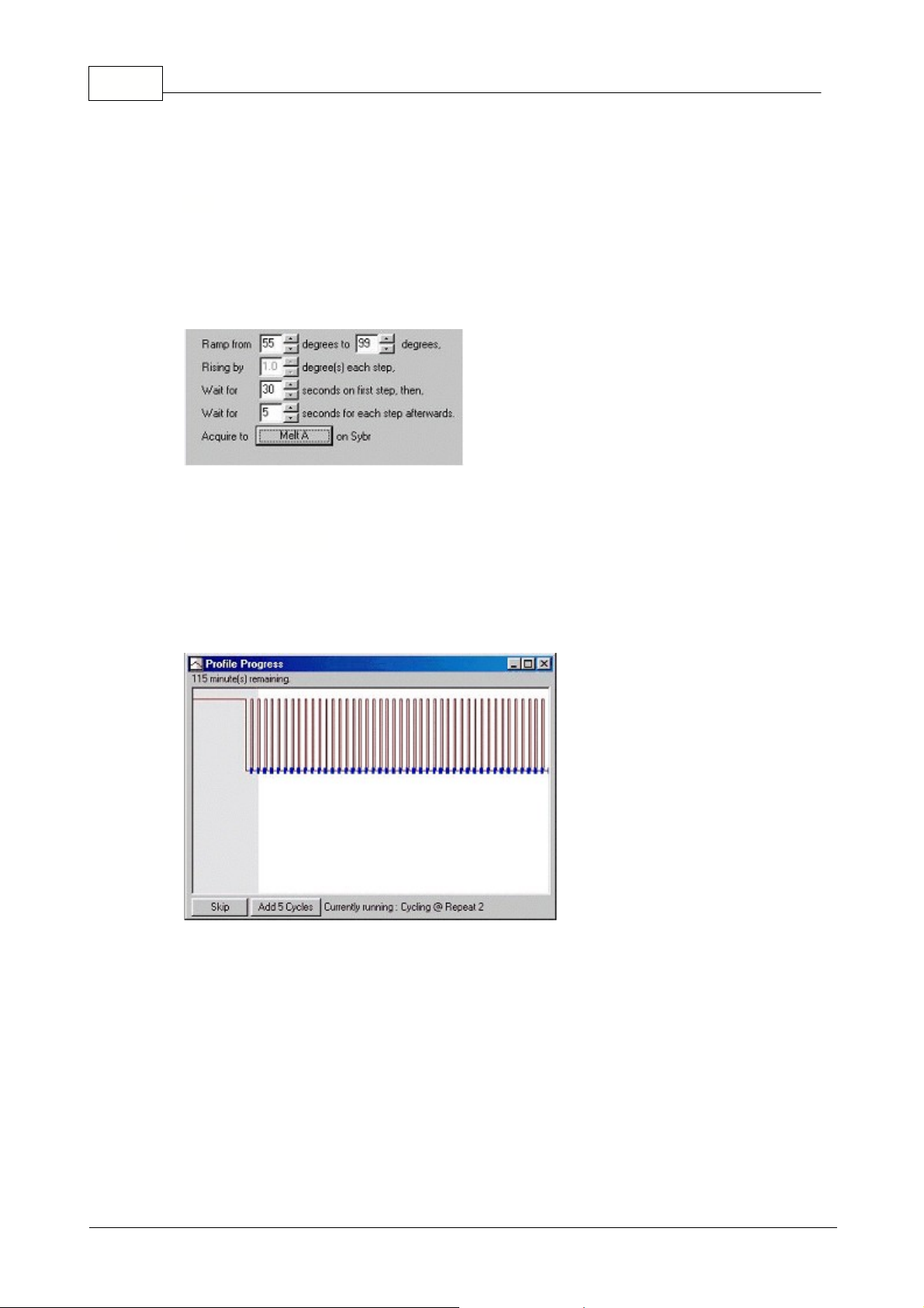
57 Rotor-Gene

put in the right-hand side will be acquired to. To not acquire on this cycle point, click on

Don't

Acquire

. Any changes you make will be reflected back on the Profile Edit window.

For a melt cycle, specify a start temperature, an end temperature, the time you want to wait at before

the first acquiring point, the amount of time to remain at each point and a ramp will be generated going

between the two temperatures. The

Acquiring To

option, here set to

Melt A

, can be changed by

clicking on the button. The same screen as for Cycling will appear and the channels to acquire to can

be selected.

When running a standard melt the temperature is increased by increments of 1ºC.

This screen shows a graphical representation of the thermal profile associated with the experiment.

When running an experiment the shaded portion of the window indicates the number of cycles that

have been completed. There is also an estimate of how many minutes the program will take to finish

this run.

There are two further buttons on the buttons,

Skip

and

Add 5 Cycles

. While skip allows skipping any

steps of the profile, the "add 5 cycles" button allows to add five cycles to the cycling profile.

Melt

5.8.4 Profile Progress

5.8.5 Edit Samples

This window has identical functionality to the sample edit grid in the New Experiment Wizard, except

that the toolbar functions are also available in the File and Edit menus. This menu can also be

accessed by right clicking over the sample list on the right side of the main screen.

Three menus are given on the top of the screen,

File, Edit

and

Help

. The file menu is used to create a

new (blank) sample sheet, open an existing sample template or save sample names as a template for

future use. The extension of those files is *.smp

Given concentration format:

This drop down menu is used to choose a concentration suitable

format. Due to the fact that different countries show formats in different ways, various formats are

given to choose from.

Unit:

This drop down menu allows choosing an appropriate unit for your assay.

Edit:

Pressing this button opens the color scheme. Selected samples (up to 36 or 72) will be changed

according to the color chosen. Click OK and all the selected samples will be assigned this color.

Reset Default:

Click this to reset all selected color cells back to their default color values.

Gradient:

The gradient function allows choosing a gradient form the first to the last selected color. A

gradient has been used in the above sample list. Several gradients can be chosen in a sample setup.

Export Samples:

To export data into an Excel spreadsheet simply use the right mouse button. Excel

will automatically be opened and exports the samples. Using the

Export Samples...

function in the

main window will also create a file that can be can exported into a spreadsheet application. Importing

samples from Excel into the Rotor-Gene software is also possible by simply using the copy and paste

58Functional Overview

59 Rotor-Gene

function.

Tab Key:

The Tab key can be used to navigate around the sample editor.

New Icon:

Clears the sample grid in preparation for data entry.

Open Icon:

Brings up a dialog box in which you can select a Rotor-Gene Sample file to import. Note:

A 32-well sample setup cannot be imported into a 72-well setup and vice versa. The number of

samples in the open sheet and the file being imported must match.

Save As Icon:

Brings up a dialog box in which you can enter the name of a file to save the current

samples to.

Copy Icon:

Copies the selected cells.

Paste Icon:

Pastes cells which had been selected with the copy command onto the currently selected

position on the grid.

Excel Icon:

Pressing the Excel icon prompts you for a file name. Excel is than opened automatically.

Sample Types:

There are several sample types listed.

Sample Type

Meaning

None

No sample in that position.

NTC

No Template Control

-ve Control

Negative Control

+ve Control

Positive Control

Sample

Unknown sample to be quantitated or melted.

Standard

Values are used to construct a standard curve to calculate

unknown sample concentrations.

Standard Sets:

This new function allows the user to choose various standard curves in the same run.

Use the arrow buttons to move from one standard set the next. The software only allows you to move

further if standards in the previous standard set have been defined.

This feature is very useful when different standard curves need to be run, either in one channel (for

example Sybr-Green I or any other fluorphore) or in different channels (with up to four different

fluorphores).

Given Conc.:

Shows the concentration for each of the standards defined. The units can be defined

as a decimal or log number. If a dilution series has to be typed in it is only necessary to type the first

two standards. By pressing ENTER, the program automatically adds the 10 fold concentration, if there

are further Standards defined below.

Line Style:

You can modify the style of the line to improve readability of graphs on black and white

printers. You can also add emphasis to certain lines by modifying their style. To access this feature,

click on the right arrow button next to the Edit button:

60Functional Overview

The toolbar will then change to show the default style "Solid". You can change this to "Dashed",

"Dotted" or a number of other possibilities. When you have finished, click the left arrow button to return

to the Edit, Reset Default and Gradient view.

Productivity Tips:

Autocompletion:

When entering standards, if you place them in consecutive tubes, begin entry on

the first tube, then press Enter. Enter the second concentration, then press Enter. The software has

automatically predicted the next concentration in the set. Keep pressing Enter to fill in the remaining

rows.

Multiple-Row Entry:

If you need to enter the same information for several rows at once, select all the

rows, then begin to type. The information will be entered into each row. This works for selecting

sample types, choosing colors or entering concentrations.

Sample Type Hotkey:

To quickly select a sample type, just enter the first letter of its name. So, to set

5 samples to be Non Template Controls, select them in the sample type column, then press N for

NTC. All samples will be converted to NTC's. NOTE: Since Sample and Standard have the same

beginning letter, press S until the one you want is selected.

Note:

A complete sample description can be saved as a sample file (*.smp) and loaded into future

experiments with the same sample configuration.

When setting up a new experiment with reactions that have not previously been run on the Rotor-Gene

it is helpful to use the Gain calibration function. This screen allows you to set the Gains of each of the

channels and the set temperature.

Note: The gain calibration will never be 100% correct. This could be due to changes in

fluorescence after the first denature step. Nevertheless, the result of the Gain calibration will

give you a good indication on what fluorescence level the run will be started.

The Gain for each channel is 1 to 10, 1 = least sensitive and 10 = most sensitive.

When running reactions for the first time it is advisable to prepare a test sample containing all reaction

components. This is then placed in the machine and Gain Calibration is run to determine the best Gain

setting.

This window lets you calibrate your machine by automatically adjusting your Gain settings until the

readings for all selected channels fall below a certain threshold. You can select to calibrate all

channels, or just those that you will be using in the current experiment.

Note: This is only available

on Rotor-Gene 3000, or the 4-channel, Multi-Filter Rotor-Gene 2000.

5.8.6 Gain Calibration

Auto-Calibration

61 Rotor-Gene

Set temperature to ...

Before reading, the machine will be heated or cooled to match the given

temperature.

Calibrate All / Calibrate Acquiring:

"Calibrate All" will attempt to calibrate for all channels known by

the software. Selecting "Calibrate Acquiring" will instead only calibrate those that you have used in the

thermal profile defined in the experiment (cycling and melt).

Channel Settings:

This is a pull down menu allowing you to add additional channels to the gain

calibration window. Choose the channel of interest and

Add.Edit...

Opens a window where the fluorescence range of the sample can be determined. The auto-

calibration process begins on Gain 5, reading from each channel. It chooses the first Gain, which has

a fluorescence reading equal to or below the level you set in this box. In the example below, tube

position 1 was chosen with a target sample range between 5 and 10 Fl.

Remove and Remove all:

Removes the highlighted channel or all channels.

62Functional Overview

Start:

Begins the calibration process. A Gain will be chosen which is within the given range. If no

value is found within the range, the closest match will be chosen.

Manual:

Opens the Manual Calibration screen (see below).

Close:

Closes this window. You cannot close the calibration window while the machine is in operation.

Perform Calibration Before 1st Acquisition:

This tick box performs the Gain calibration at the first

cycle where data acquisition occurs. This is useful as with some probes after the initial denaturation

the background fluorescence of the probes could change substantially.

Perform Calibration At [x] Degrees At Beginning of Run:

This tick box performs the Gain

calibration just before starting the experiment. The machine is heated to the given temperature, the

gain calibration is performed, and then cycling begins on the first step, usually a Denature. This can

be useful when a calibration during the run may impact too much on the time spent on the initial step.

Usually, however,

Perform Calibration Before 1st Acquisition

should be the ideal option as

calibration is performed as close as possible to experiment conditions.

Changing Gain During a Run:

If the Gain at the beginning of the run was accidentally chosen to

high or to low it can be changed within the first ten cycles. A vertical line in the main screen will appear

where the Gain has been changed. Due to the drop or increase in fluorescence the cycles before the

change will be excluded from the analysis.

This window lets you view in real time the fluorescent readings at any given temperature. It is used

when the background of a sample is unknown and therefore the Gain has to be determined to ensure

the sample signal is sufficiently on scale.

By default, the first eight samples are toggled on. If more than the first samples would like to be

monitored, turn on the samples of interest. Using manual gain calibration means that data are always

from all samples.

It takes approximately 4 seconds to acquire data per channel. During this time the user interface is

inactivated and so it is best to 1) Start the test 2) wait for the temperature to stabilize 3) note the end

point fluorescence (Fl) reading 4) stop the unit 5) make the appropriate Gain change 6) and restart the

unit.

Manual Calibration

63 Rotor-Gene

Temperature:

Change this value to set the temperature of the machine. Note: The temperature will

only be sent when the start button is pressed. Adjust the temperature on the Gain calibration screen to

reflect the required acquisition temperature for the run.

Edit Gains:

Opens the Edit Gains window. The Gains will be sent the next time the machine is started

in the calibrate window.

Start:

Begins the run, setting the machine temperature to that displayed on the screen. The

temperature and channel graphs will start to display data. Ensure the Rotor-Gene displays READY

before starting another calibration run.

Stop:

Stops the experiment. If the experiment is still acquiring data when you click the button, then the

machine will first finish acquiring, and then stop the machine. This process can take up to 5 seconds

for each channel data is being acquired.

NOTE: The aim of the Gain setting is to have all data on the screen. The Gain doesn't

influence your data. If the Gain was chosen too high, curves might go off scale and data

could be lost. It is therefore a good idea to start a Sybr-Green I or dual-labeled probe run with

a low fluorescence (an increase is expected) and a quenched FRET run with a higher

fluorescence (a decrease is expected).

Show at most two analysis windows:

This option ticked shows a maximum of two analysis

windows at once. By performing a quantitation analysis, three windows are opened by default. If more

than six or seven windows are opened at once, the overall view might not be clear. This option ticked

will close the first analysis window and replace it with the last opened analysis window. If the option is

unticked more than three analysis windows could be displayed. This could be useful when comparing

quantitation screens of four different channels.

Show at most 6 windows:

To improve readability, the software removes unused windows when new

windows are opened. This option is enabled by default, as it keeps the Rotor-Gene work area clear.

You may, however, need to see more than 6 windows at once, in which case you should uncheck this

option.

5.8.7 Display Options

Reset all "Don't Show This Message again" Dialogs:

This window forces the software to re-

display all dialog boxes again. These include messages about suspicious settings which you may have

previously set to not display again. This might be useful if a new user is now using the machine who is

unfamiliar with the Rotor-Gene or the Rotor-Gene software.

5.9 Gain Menu

Here, you can view the

Gain Settings

for the current experiment and modify them if the experiment

has not yet been run. Use the

Up/Down

arrows next to each text field to modify the fields without

needing to enter in a value with the keyboard. Click OK when you have finished.

Sets the Gain of the specified channel before running a program. Gain settings will be retained from

the last run.

Change gain during the first ten cycles:

This new software version also offers the possibility to

change the gain during the initial cycles. A red line will be drawn in the appropriate channel showing

where the gain has been changed. The cycles before the gain has been changed will be excluded of

the calculation of the quantitation data.

Note: This is only possible for 4-Channel Rotor-Gene, not for dual channel or 32-well Rotor-

Genes.

This menu allows you to tile the window either vertically, horizontally or arrange windows in a cascade.

A further option of tiling windows is found under Arrange in the tool menu.

The

Contents

contains all the help files sorted by names. Simply go to contents and choose the area

you are interested in.

What' New

gives a brief overview of new features added to the previous software

release.

Context Sensitive Help

will open the help file according to the activated window in the Rotor-

Gene software. Pressing

Corbett Research Website

will automatically open our Web page, whereas

the forum can be accessed by pressing

Rotor-Gene Online Forum

About Rotor-Gene

tells you

several details for example the serial number of the Rotor-Gene or the software version you are using.

64Functional Overview

5.10 Window Menu

5.11 Help Menu

65 Rotor-Gene

The

Send Support Email

option in the Help menu allows you to send a support email to Corbett

Research which contains all relevant information to an experiment. The

Save As option

will save all

the information to a file which you can copy onto a floppy disk or onto a network if you do not have

access to email on the Rotor-Gene machine.

While running an experiment, a second already finished experiment can be opened and analyzed. Note

that several functions like

New

Start Run

are not activated in this second window. Even closing the

first experiment will not bring up those functions. A new run can only be started from the first

experiment, once the experiment has finished. If a run has to be started from the second experiment, it

needs to be closed and reopened to access the appropriate functions.

5.11.1 Send Support E-Mail

6 General Functions Used Over Several Windows

6.1 Opening A Second Experiment

6.2 Spanner Icon

By clicking the spanner icon, you have access to a number of tools, which simplifies manual analysis

of data. Those tools could also be accessed using the right mouse button in the appropriate screens.

Scaling:

See above

Export to JPEG...

Saves the graph in the JPEG image format and

Export to BMP...

saves the graph

in the Bitmap format.

Print:

This function allows for the current graphic screen to be printed.

Digital Filter:

Modifies the currently selected digital filter on the graph. The digital filter smoothes data

using a sliding window of points. To open the window, click the right mouse button over a window

containing data.

Show Pinpointer:

Opens a window with exact coordinates of the current cursor position.

Note: The following options are no longer available via the Spanner icon. You should first

drag a selection area on the graph, and then, upon releasing the mouse, a context menu will

appear. Choose one of the following options to select samples or zoom the graph.

Select Samples:

Shows only the samples that you swipe in a rectangular region.

Zoom:

With the zoom function you can zoom in certain areas of the screen. It can be horizontally and

vertically.

66General Functions Used Over Several Windows

67 Rotor-Gene

Adjust Scale

will bring up a window in which you can manually enter a scale, or interactively select

one. To chose this option simply press the right mouse button over the appropriate screen.

BHQ

Black Hole Quencher

Comp. Quantitation

Comparative Quantitation

LCD

Liquid crystal display

LED

Light Emitting Diode

PMP

Photomultiplier

Quant.

Settings

Quantitate Settings

REA

Rotor-Gene Archive File

REX

Rotor-Gene Experiment File

Rotor-Gene

SMP

Sample File

Std. Curve

Standard Curve

Auto-Scale

attempts to fit the scale to the maximum and minimum readings in the data.

Default:

will reset the scale to show from 0-100 fluorescence units.

6.3 Scaling Options

6.4 Abbreviations

6.5 Auto-Scale

7 Quick Start Using The New Experiment Wizard

To perform a new experiment, click on the New icon .

By default the setup Wizard is active and you should see the wizard screen appear. If the Wizard does

not appear tick the appropriate box in New Experiment.

The wizard comes up with a welcome screen. After reading the introduction, the box

Skip this

introductory screen in the future

can be ticked. The welcome screen will then automatically be

skipped in the future.

7.1 Welcome Screen

68Quick Start Using The New Experiment Wizard

69 Rotor-Gene

The setup wizard guides you through all the necessary steps to setting up an experiment.

7.2 Page 1

7.3 Page 2

In this screen the

Temperature Profile

and the

Channel Setup

can be modified. Simply press the

appropriate buttons and modify as outlined in previous chapters.

70Quick Start Using The New Experiment Wizard

71 Rotor-Gene

The last screen gives a summary of what you are about to run. Always check the parameters. If you

are satisfied with the parameters click

Start Run

and you will be prompted for a file name. Before

starting the run make sure that the Rotor-Gene is in

READY

mode.

NOTE: If the unit does not display READY on the LCD screen, the detectors will not be

activated and no data will be collected.

7.4 Page 3

7.5 Page 4

Once the experiment has begun, you can enter in sample types and descriptions while you wait for it to

complete. The functionality of this screen is identical to the

Sample Editor

Filter specs:

Channel 1

Excitation:

470nm

Detection:

510nm

Channel 2

Excitation:

530nm

Detection:

555nm

Sybr-Green I

is detected on Channel 1

Dual labeled probes

can be detected on Channel 1 and Channel 2, when labeled with FAM or JOE

(VIC), respectively.

Quenchers

for the above fluorophores could be BHQ1 or TAMRA.

FRET style quenched probes

could also be used labeled with FAM and JOE (VIC).

72Quick Start Using The New Experiment Wizard

8 Rotor-Gene Hardware Information

8.1 Filter Specifications

8.1.1 32 Well and Dual-Channel Machines

73 Rotor-Gene

NOTE: The above quenched dyes can be multiplexed in the same tube with no cross-talk in

Channel 1 and less than 1% cross-talk in Channel 2.

Sybr-Green I

is detected on Channel 1 (FAM Channel) or Sybr Channel.

Dual Labeled Probes

Fluorophores

Excitation

Emission

Filter-Setup

5-FAM, 6-FAM:

495

520

FAM Channel

JOE

520

548

JOE Channel

TET

521

536

JOE Channel

HEX

535

556

JOE Channel

Cy3

550

570

470/585 hp or 530/585 hp

TAMRA

555

576

530/585 hp

Cy3.5

581

596

ROX Channel

ROX

575

602

ROX Channel

Red 640

625

640

Cy5 Channel

Cy5

649

670

Cy5 Channel

For multiplex reactions we recommend using FAM, JOE, ROX and Cy5, since those fluorophores after

optimization give a cross talk less then 1%.

Quenchers

to be used for the above dyes:

BHQ-1:

480 – 580

BHQ-2:

550 – 650

BHQ-3:

620 – 730

TAMRA for FAM or JOE (VIC)

8.1.2 Multi-Channel Machines

FRET Analysis

FAM and JOE for example have to be detected on the above mentioned channels (quenched FRET).

If Cy5 has to be detected (normal FRET) the filter combination must be as follows:

FAM-Cy5, FAM-LC 640, FAM-

LC 705

470/610 hp

FAM-BHQ1:

FAM Channel

JOE-Cy5

530/610 hp

JOE-BHQ1:

JOE-Channel

9 Troubleshooting

The software keeps an untouched copy of each experiment, along with diagnostic information in its

Log Archive repository. By using the Help, Send Support Email option, you can send an email with all

the diagnostic information the Corbett Research support technicians require:

Previously, customers were required to send the experiment file, the temp.log and rot.log files. This is

no longer necessary.

To troubleshoot experiments which did not occur as expected, enter the Profile Editor and ask the

following questions:

9.1 Log Archives

74Rotor-Gene Hardware Information

9.2 Troubleshooting Experiment Files

75 Rotor-Gene

Is the initial denature temperature and time for the Taq Polymerase used appropriate?

Check

the manufacture's description of the enzyme. The recommended temperature is 95°C and the times

can vary from 2 min to 15 min, depending on the enzyme used. If genomic DNA has been used for the

assay, the initial denature time should be at least 5 min depending on how the DNA has been

extracted.

Have 50 ml volumes been run on the Rotor-Gene?

The Rotor-Gene is calibrated for 20 – 25

l, in which case we recommend a denaturation time during

cycling of 15 seconds. Some protocols specify 50

l reactions in which case we recommend

increasing the denaturation time during cycling to 30 seconds.

Is the denature temperature appropriate?

Most double stranded DNA has melted at 95°C. In some

cases temperatures from 90°C to 94°C may not denature the DNA properly. Due to partially denatured

DNA, the accessibility of primers and probes could be reduced and could therefore reduce the

reaction efficiency of the assay.

Is the denature time appropriate?

15 to 20 sec is usually enough to denature the amplicon,

however, longer products might need up to 30 sec. A denature time of 60 sec is usually not required.

Is the annealing temperature and time appropriate?

Check the Tm's of the primers and probes.

The annealing time for Sybr-Green I is around 20 to 35 sec. Dual labeled probes are often run as a

two step profile where annealing and extension steps are combined. In this case the

annealing/extension step is between 45 and 60 sec and the temperature is usually 60°C. For FRET

probes the annealing step is between 20 and 30 sec.

Is the extension temperature and time appropriate?

Check the recommendations of the

manufacturer's Taq Polymerase. For a product less than 300 bp the recommended time is between 15

and 30 sec.

At what step have data been acquired?

For Sybr-Green I data should be acquired at 72°C. This is

where most of the DNA is expected to be double stranded. As mentioned above, dual labeled probes

are often run as two step assays. Data therefore should be acquired at the anneal/extension step. For

FRET assays, data should be acquired at the annealing step. If in doubt about the appropriate data

acquisition point, data could be acquired at several steps for comparison. If no raw data can been seen

on the screen at all, go to edit profile and check if data was acquired at least at one point.

Has a hold step at the same temperature as the beginning of the melt been inserted before

starting the melt curve?

If no hold step has been used before running a melt curve, the results in the

melt curve analysis could be a steep increase in the first few cycles making the actual melt peak hardly

visible.

For Sybr-Green I melt curves; was the melt curve run to 99°C?

Some amplicons melt higher than

90°C. The expected melt peak might not occur, due to the fact that DNA has not melted.

9.2.1 Initial Denature Step

9.2.2 Cycling Profile

9.2.3 Melt Curve Analysis

9.2.4 Gain Settings

Have the appropriate gain settings been chosen?

In some cases it has been observed that curves

in the raw data went off scale resulting in a straight line at a fluorescence of 100. Although quantitation

of most data could still be performed, the gain should be reduced to a setting, where the raw data does

not go off scale.

In some cases it has been observed that the fluorescence went off scale up from the first cycle. This

is due to the fact that the gain setting was chosen too high. It might look like that no data has been

acquired.

If a straight line at a fluorescence of 100 at the beginning of a melt curve is observed, the melt curve

should be rerun using a lower gain. There is no need to rerun the amplification, Sybr-Green I or FRET

samples can be reused to a certain extent.

Has the appropriate Quantitation Setting been chosen?

In some cases it has been observed that

the raw data show a perfect amplification but no data could be seen in the quantitation screen. Setting

the Quantitation Setting to zero will show all data. The Quantitation Setting can be used to exclude

small changes of fluorescence, due to probe degradations or other probe related effects, which do not

show true amplification but rather a steadily increasing line.

If the quantitation curves can be excluded with a minimal Quantitation Setting the gain for the next run

should be increased. Note: the gain setting has no influence on the actual data, the expected fold

increase will be similar.

Has the appropriate setup been chosen for the Rotor-Gene?

To check, go to file menu then to

setup and tick the appropriate boxes. If in doubt what each of the boxes means or if setup is not

accessible, please contact the distributor.

Has the appropriate rotor for the run been chosen?

Before running an experiment make sure that

either the 36 or 72 well rotor has been chosen according to the rotor in the Rotor-Gene. Choosing the

wrong rotor might either result in not acquiring every second sample (running 72 well rotor but 36 well

setup was chosen) or acquiring double the amount of data that is actually in the rotor (running 36 rotor

but 72 setup was chosen).

What version of the software is used on the Rotor-Gene?

The software development for the

Rotor-Gene is ongoing and freely downloadable from the Corbett Research web page

(

www.corbettresearch.com

)

. Make sure that a recent version is uploaded and used.

If samples are not detected check also the channel setup. Make sure data has been acquired with the

appropriate excitation and detection filters. This is particularly important when user defined filters have

been setup.

Depending on the environment in which the Rotor-Gene is setup, spikes could be caused due to the

noise from mains. The Rotor-Gene software has a build in spike suppression and will tell the user if

spikes occurred during a run. If normal or medium spike suppression does not suppress spikes, high

spike suppression should be ticked (version 4.4 or less). More recent versions have only one option to

suppress spikes, by either enabling or disabling spike suppression. Spike suppression (high) is

recommended and can be chosen in the experiment wizard.

What if all the above mentioned conditions were right, but the assay did not look as expected

or did not work at all?

In the restricted area of our homepage there is a file called "real-time

76Troubleshooting

9.2.5 General Setup Conditions

9.2.6 Experiment Settings

77 Rotor-Gene

summary". Steps are suggested on how to optimize Sybr-Green I, dual labeled probes and FRET

reactions. In general, the expected fold increase of a Sybr-Green I reaction is between 5 and 50 times

and a dual labeled reaction between 2 and 10 times.

On some computers, the regional settings are configured in a contradictory manner which causes a

conflict within the Rotor-Gene system. The problem occurs when different decimal settings are used

for curencies and numbers. For example, if numbers are displayed in a "123 456,789" format, but

currencies are shown as "$299,192.20", then there is a conflict, since the number "20,123" is

ambiguous. On Windows 98 machines, this prevents the Rotor-Gene software from correctly

interpreting numbers. This problem does not occur on Windows 2000.

To correct this setting, please follow the following steps. The names of these options may be different

in your system's language.

Click on the Start Menu.

Click on Settings.

Click on Control Panel.

Double-Click on Regional Settings.

Double-Click on Regional Options.

Click on the Numbers tab.

Note down which is the Decimal Symbol, and which is used as the Digit Grouping Symbol. On a

German system, for example, the comma (,) will be used for Decimals, and the period (.) is used as

a Digit Grouping Symbol.

Click on the Currency tab.

Change the Decimal Symbol and the Digit Grouping Symbol to be the same as on the Numbers tab.

Click OK.

Re-run the Rotor-Gene software.

To run software with the Rotor-Gene 3000 you have to follow these steps:

1. Setting up the Rotor-Gene 3000 Software for the first time:

Insert the Rotor-Gene 3000 CD into your CD drive.

Double Click on My Computer icon.

Double Click on Compact Disc Rotor-Gene 3000.

Double Click on RgSetup folder.

Double Click on executable file Rotor-Gene_X_Y_ZZ.exe (where X is Major version number, Y is Minor

version number, ZZ is Revision version number).

Follow all Installer instructions.

2. Setting up the Rotor-Gene 3000 Software on a PC where it was already installed.

If you install Rotor-Gene 3000 Software on PC where it was installed before, it is necessary to

uninstall any previous version of Rotor-Gene on your system.

In order to uninstall Rotor-Gene Software:

Click on Start button on Taskbar,

choose Settings, choose Control Panel, double click on Add/Remove Programs icon, choose Rotor-

9.3 Regional Settings In Windows 98

10 Rotor-Gene 3000 Setup Instructions

Gene

Click Change/Remove

Click Yes.

Then, to reinstall:

Insert the Rotor-Gene 3000 CD into your CD drive.

Double Click on My Computer icon.

Double Click on Compact Disc Rotor-Gene 3000.

Double Click on RgSetup folder.

Double Click on executable file Rotor-Gene_X_Y_ZZ.exe (where X is Major version number, Y is

Minor version number, ZZ is Revision version number).

11 Rotor-Gene 2000 Setup Instructions

To run software with Rotor-Gene you have to follow through these steps from 1-8 to install the board,

the software drivers and the Rotor-Gene Software.

To run the software with the Rotor-Gene the Virtual Machine must not be ticked.

If you want to install a demonstration version of Rotor-Gene Software you have to do Step 7 only

(Installing the Rotor-Gene Software). When you run software for demonstration purposes leave Virtual

Machine ticked.

In order to change Virtual Machine box must click <File> <Setup> on the main Rotor-Gene Software

screen.

If you Install Rotor-Gene Software on PC running Windows 95/98 you must

disable Interrupt 3 in BIOS.

Boot the computer and Press Delete on keyboard simultaneously.

Choose INTEGRATED PERIPHERALS.

Change On Board Serial Port2: Disabled (Could be different on different PC i.e. Onboard Serial Port2

: 2F8/IRQ3)

Exit and Save Changes

If you install the Rotor-Gene Software on PC running Windows NT you must disable Interrupt 3 in

BIOS.

Removing Com Port 2

Click on the Start Menu, Settings and Control Panel

Double-click on System. Then select the second tab Device Manager.

Click on the [+] sign next to Ports(COM+LPT) then click on COM2 If it still exist there.

Click on Properties.

Tick Disable in this hardware profile and click OK.

Click Close for Device Manager.

Reboot computer.

Disable hard disk power down

Click on the Start Menu, Settings and Control Panel

Double Click on Power Management

Choose Never for hard disks

Installing the Data Acquisition board

78Rotor-Gene 3000 Setup Instructions

79 Rotor-Gene

Set the Interrupt jumper on the board to IRQ3.

Turn of the computer.

Plug in the board.

Turn on your computer again.

Installing the Computer Boards Software

Insert the Rotor-Gene 2000 CD into your CD drive.

Click on Start, Run.

Type in D:\RG2000\UNIVLIB5.04\DISK1\SETUP.EXE then press ENTER. If the drive letter of your

CD Rom is one other than D, replace D with that drive letter.

The installation software will now start up. An screen will ask you to select which files to install. Select

ONLY "Win 95/98/NT 32-bit Universal Library and Instacal", unticking any other options.

When the software asks you if it can make changes to AUTOEXEC.BAT, select "Yes". Do likewise for

SYSTEM.INI.

The software will then ask you if it can reboot the computer. Select Yes.

Configuring The Computer boards Software

Click on Start, Run.

Type c:\cb\inscal32.exe and click OK.

Click on Install, Add Board…

Select the board CIO-DAS802 and click OK.

Double-click on the CIO-DAS802 board.

Set the Interrupt Level to 3.

Set Wait State Disabled.

For each Channel from 0 to 7 in channel configuration, change from DIFF to SE.

Click OK.

Select File, Exit.

Installing the Rotor-Gene Software

If you install Rotor-Gene Software first time go to 7.a .

Before installing any new version of the software, it is necessary to uninstall any previous version of

Rotor-Gene on your system.

Click on Start, Settings, Control Panel.Double click on Add-remove software.

In the list box at the bottom of the window, for each copy of Rotor-Gene in the list, click on Rotor-

Gene, then click on Add/Remove. Click on Close.

You can now run setup.exe, located in D:\ RGSetup\Setup.exe

If the drive letter of your CD Rom is one other than D, replace D with that drive letter.

12 Rotor-Gene 2000 IMPORTANT SETTINGS

IMPORTANT SETTINGS THAT SHOULD NOT

BE CHANGED ON THE PC

DO NOT Turn off hard disks. Ensure Power-down on hard disks is set

to NEVER.

DO NOT Put the system on Standby. Ensure Enter Standby mode is set

to NEVER.

DO NOT Install any peripheral devices that are using Interrupt 3.

DO NOT Install computer on network if the network card is using

Interrupt 3.

DO NOT Enable Interrupt 3 in BIOS.

DO NOT install custom screen savers.

NB: These notes only apply to the Rotor-Gene 2000.

80Rotor-Gene 2000 IMPORTANT SETTINGS

Eppendorf Rotor-Gene Software manual

Specifications and Main Features

Frequently Asked Questions

User Manual