Bio-Rad Firmware Software Updates User Manual

Download

MiniOpticon™ System

Instruction Manual

For MiniOpticon real-time PCR detection

™

system with CFX Manager

Catalog #CFB-3120

software

Adobe, Acrobat, and Reader are trademarks of Adobe Systems Incorporated. Excel, Microsoft, Windows, and Windows Vista are trademarks of Microsoft Corporation. EvaGreen is a trademark of Biotium, Inc. Bio-Rad Laboratories, Inc., is licensed by Biotium, Inc., to sell reagents containing EvaGreen dye for use in real-time PCR, for research purposes only. FAM, HEX, VIC, and ROX are

trademarks of Applera Corporation. SYBR® is a trademark of Life Technologies Corporation. Bio-Rad

Laboratories, Inc. is licensed by Life Technologies Corporation to sell reagents containing SYBR® Green for use in real-time PCR, for research purposes only.

LICENSE NOTICE TO PURCHASER

Purchase of this instrument conveys a limited non-transferable immunity from suit for the purchaser's own internal research and development and for use in human in vitro diagnostics and all other applied fields under one or more of U.S. Patents Nos. 5,656,493, 5,333,675, 5,475,610 (claims 1, 44, 158, 160-163 and 167 only), and 6,703,236 (claims 1-7 only), or corresponding claims in their non-U.S. counterparts, owned by Applera Corporation. No right is conveyed expressly, by implication or by estoppel under any other patent claim, such as claims to apparatus, reagents, kits, or methods such as 5' nuclease methods. Further information on purchasing licenses may be obtained by contacting the Director of Licensing, Applied Biosystems, 850 Lincoln Centre Drive, Foster City, California 94404, USA.

Bio-Rad’s real-time thermal cyclers are licensed real-time thermal cyclers under Applera’s United States Patent No. 6,814,934 B1 for use in research, human in vitro diagnostics, and all other fields except veterinary diagnostics.

This product is covered by one or more of the following U.S. patents, their foreign counterparts, or their foreign counterparts owned by Eppendorf AG: U.S. Patent Nos. 6,767, 512 and 7,074,367.

Bio-Rad Resources

Table 1 lists Bio-Rad resources and how to locate what you need.

Table 1. Bio-Rad resources

Resource How to Contact

Local Bio-Rad Laboratories representatives

Technical notes and literature Go to the Bio-Rad website (www.bio-rad.com). Type a

Technical specialists Bio-Rad’s Technical Support department is staffed with

Find local information and contacts on the Bio-Rad website by selecting your country on the home page (www.bio-rad.com). Find the nearest international office listed on the back of this manual.

search term in the Search box and select Documents tab to find links to technical notes, manuals, and other literature.

experienced scientists to provide customers with practical and expert solutions. To find local technical support on the phone, contact your nearest Bio-Rad office. For technical support in the United States and Canada, call 1-800-4246723 (toll-free phone), and select the technical support option.

Writing Conventions Used in this Manual

This manual uses the writing conventions listed in Table 2.

Table 2. Conventions used in this manual

Convention Meaning

TIP: Provides helpful information and instructions, including information

explained in further detail elsewhere in this manual.

NOTE: Provides important information, including information explained in

further detail elsewhere in this manual.

WARNING! Explains very important information about something that might

damage the researcher, damage an instrument, or cause data loss.

X > Y Select X and then select Y from a toolbar, menu or software window.

For information about safety labels used in this manual and on the MiniOpticon system, see, “Safety and Regulatory Compliance” on page iii.

MiniOpticon Instruction Manual

Safety and Regulatory Compliance

For safe operation of the MiniOpticon system, we strongly recommend that you follow the safety specifications listed in this section and throughout this manual.

Safety Warning Labels

Warning labels posted on the instrument and in this manual warn you about sources of injury or harm. Refer to Table 3 to review the meaning of each safety warning label.

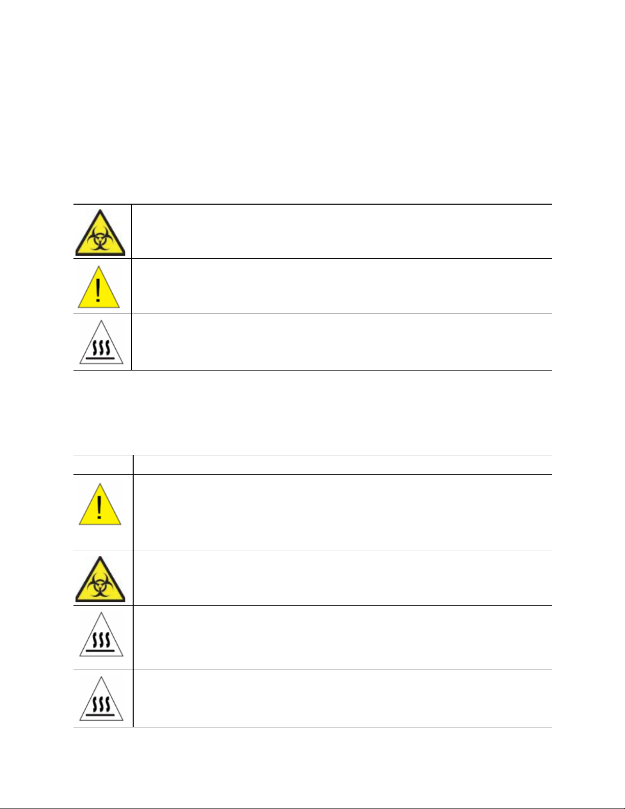
Table 3. Meaning of safety warning labels

CAUTION: Biohazard! This symbol identifies components that may become contaminated

with biohazardous material.

CAUTION: Risk of danger! This symbol identifies components that pose a risk of personal injury or damage to the instrument if improperly handled. Wherever this symbol appears, consult the manual for further information before proceeding.

CAUTION: Hot surface! This symbol identifies components that pose a risk of personal injury due to excessive heat if improperly handled.

Instrument Safety Warnings

The warning labels shown in Table 4 also display on the instrument, and refer directly to the safe use of the MiniOpticon real-time PCR detection system.

Table 4. Instrument Safety Warning Labels

Icon Meaning

Warning about risk of harm to body or equipment.

Operating the MiniOpticon real-time PCR detection system before reading this manual can constitute a personal injury hazard. For safe use, do not operate this instrument in any manner unspecified in this manual. Only qualified laboratory personnel trained in the safe use of electrical equipment should operate this instrument. Always handle all components of the system with care, and with clean, dry hands.

CAUTION: Biohazard! This symbol identifies components that may become contaminated with biohazardous material.

Warning about risk of burning. A thermal cycler generates enough heat to cause serious burns. Wear safety goggles or other eye protection at all times during operation. Always allow the sample block to return to idle temperature before opening the lid and removing samples. Always allow maximum clearance to avoid accidental skin burns.

Warning about risk of explosion. The sample blocks can become hot enough during the course of normal operation to cause liquids to boil and explode.

iii

Safe Use Specifications and Compliance

Table 5 lists the safe use specifications for the MiniOpticon system. Shielded cables (supplied) must be used with this unit to ensure compliance with the Class A FCC limits.

Table 5. Safe Use Specifications

Safe Use Requirements Specifications

Indoor use. The system will operate safely when the ambient temperature is 5 — 40oC and will meet performance

Temperature

Altitude Up to 2,000 meters above sea level

specifications when the ambient temperature is 15—31oC with a maximum relative humidity of 80% for temperatures up to 31oC, decreasing linearly to 50% relative humidity at 40oC

Electrical supply

Installation categories (Overvoltage Categories) II

Pollution degree 2

100—240 VAC, 50—60 Hz, 400W. Main supply voltage fluctuations not to exceed +/- 10% of nominal voltage

REGULATORY COMPLIANCE

This device complies with Part 15 of the FCC Rules. Operation is subject to the following two conditions: (1) this device may not cause harmful interference, and (2) this device must accept any interference received, including interference that may cause undesirable operation.

This device has been tested and found to comply with the EMC standards for emissions and susceptibility established by the European Union at time of manufacture.

This digital apparatus does not exceed the Class A limits for radio noise emissions from digital apparatus set out in the Radio Interference Regulations of the Canadian Department of Communications.

LE PRESENT APPAREIL NUMERIQUE N’EMET PAS DE BRUITS RADIOELEC¬TRIQUES DEPASSANT LES LIMITES APPLICABLES AUX APPAREILS NUMERIQUES DE CLASS A PRESCRITES DANS LE REGLEMENT SUR LE BROUILLAGE RADIOELECTRIQUE EDICTE PAR LE MINISTERE DES COMMUNICATIONS DU CANADA.

This equipment generates, uses, and can radiate radio frequency energy and, if not installed and used in accordance with the instruction manual, may cause harmful interference to radio communications. Operation of this equipment in a residential area is likely to cause harmful interference in which case the user will be required to correct the interference at his own expense.

FCC WARNING

NOTE: Changes or modifications to this unit not expressly approved by the party responsible for compliance could void the user’s authority to operate the equipment.

This equipment has been tested and found to comply with the limits for a Class A digital device, pursuant to Part 15 of the FCC Rules. These limits are designed to provide reasonable protection against harmful interference when the equipment is operated in a commercial environment. This equipment generates, uses, and can radiate radio frequency energy and, if not installed and used in accordance with the instruction manual, may cause harmful interference to radio communications. Operation of this equipment in a residential area is likely to cause harmful interference in which case the user will be required to correct the interference at his own expense.

MiniOpticon Instruction Manual

Although this design of instrument has been tested and found to comply with Part 15, Subpart B of the FCC Rules for a Class A digital device, please note that this compliance is voluntary, for the instrument qualifies as an “Exempted device” under 47 CFR § 15.103(c), in regard to the cited FCC regulations in effect at the time of manufacture.

Hazards

The MiniOpticon real-time PCR detection system is designed to operate safely when used in the manner prescribed by the manufacturer. If the MiniOpticon system or any of its associated components are used in a manner not specified by the manufacturer, the inherent protection provided by the instrument may be impaired. Bio-Rad Laboratories, Inc. is not liable for any injury or damage caused by the use of this equipment in any unspecified manner, or by modifications to the instrument not performed by Bio-Rad or authorized agent. Service of the MiniOpticon system should be performed only by Bio-Rad personnel.

Biohazards

The MiniOpticon system is a laboratory product. However, if biohazardous samples are present, adhere to the following guidelines and comply with any local guidelines specific to your laboratory and location.

PRECAUTIONS

• Always wear laboratory gloves, coats, and safety glasses with side shields or goggles

• Keep your hands away from your mouth, nose and eyes

• Completely protect any cut or abrasion before working with potentially infectious materials

• Wash your hands thoroughly with soap and water after working with any potentially infectious material before leaving the laboratory

• Remove wristwatches and jewelry before working at the bench

• Store all infectious or potentially infectious material in unbreakable, leak-proof containers

• Before leaving the laboratory, remove protective clothing

• Do not use a gloved hand to write, answer the telephone, turn on a light switch, or touch anything that other people may touch without gloves

• Change gloves frequently. Remove gloves immediately when they are visibly contaminated

• Do not expose materials that cannot be properly decontaminated to potentially infectious material

• Upon completion of the operation involving biohazardous material, decontaminate the work area with an appropriate disinfectant (for example, a 1:10 dilution of household bleach)

• No biohazardous substances are exhausted during normal operations of this instrument

SURFACE DECONTAMINATION

WARNING! To prevent electrical shock, always turn off and unplug the instrument prior to performing

decontamination procedures.

The following areas can be cleaned with any hospital-grade bactericide, virucide, or fungicide disinfectant:

• Outer lid and chassis

• Inner reaction block surface and reaction block wells

• Control panel and display

To prepare and apply the disinfectant, refer to the instructions provided by the product manufacturer. Always rinse the reaction block and reaction block wells several time with water after applying a disinfectant. Thoroughly dry the reaction block and reaction block wells after rinsing with water.

WARNING! Do not use abrasive or corrosive detergents or strong alkaline solutions. These agents can scratch surfaces and damage the reaction block, resulting in loss of precise thermal control.

DISPOSAL OF BIOHAZARDOUS MATERIAL

The MiniOpticon system contains no potentially hazardous chemical materials. Dispose of the following potentially contaminated materials in accordance with laboratory local, regional and national regulations:

• Clinical samples

• Reagents

• Used reaction vessels or other consumables that may be contaminated

Chemical Hazards

The MiniOpticon system contains no potentially hazardous chemical materials.

Explosive or Flammability Hazards

The MiniOpticon system poses no uncommon hazard related to flammability or explosion when used in a proper manner as specified by Bio-Rad Laboratories.

Electrical Hazards

The MiniOpticon system poses no uncommon electrical hazard to operators if installed and operated properly without physical modification and connected to a power source of proper specification.

Transport

Before moving or shipping the MiniOpticon system, decontamination procedures must be performed. Always move or ship the MiniOpticon system with the supplied packaging materials that will protect the instrument from damage. If appropriate containers cannot be found, contact your local Bio-Rad office.

Storage

The MiniOpticon system can be stored under the following conditions:

• Temperature range: –20 to 60oC

• Relative humidity: maximum 80%

Disposal

The MiniOpticon real-time PCR detection system contains electrical or electrical materials; it should be disposed of as unsorted waste and must be collected separately according to the European Union Directive 2002/96/CE on waste and electronic equipment —WEEE Directive. Before disposal, contact your local Bio-Rad representative for country-specific instructions.

Bio-Rad Resources . . . . . . . . . . . . . . . . . . . . . . . . . . . . . . . . . . . . . . . . . . . . . . . . . . ii

Writing Conventions Used in this Manual . . . . . . . . . . . . . . . . . . . . . . . . . . . . . . . . . ii

Safety and Regulatory Compliance . . . . . . . . . . . . . . . . . . . . . . . . . . . . . . . . . . . . . iii

Hazards . . . . . . . . . . . . . . . . . . . . . . . . . . . . . . . . . . . . . . . . . . . . . . . . . . . . . . . . . . v

MiniOpticon Instruction Manual

Chapter 1. System Installation . . . . . . . . . . . . . . . . . . . . . . . . . . . . . . . . . . . . 1

System Overview . . . . . . . . . . . . . . . . . . . . . . . . . . . . . . . . . . . . . . . . . . . . . . . . . . . 1

System Requirements . . . . . . . . . . . . . . . . . . . . . . . . . . . . . . . . . . . . . . . . . . . . . . . 3

Setting Up the system . . . . . . . . . . . . . . . . . . . . . . . . . . . . . . . . . . . . . . . . . . . . . . . 4

Running Experiments. . . . . . . . . . . . . . . . . . . . . . . . . . . . . . . . . . . . . . . . . . . . . . . . 8

Chapter 2. CFX Manager™ Software . . . . . . . . . . . . . . . . . . . . . . . . . . . . . . 9

Main Software Window . . . . . . . . . . . . . . . . . . . . . . . . . . . . . . . . . . . . . . . . . . . . . . 9

Startup Wizard . . . . . . . . . . . . . . . . . . . . . . . . . . . . . . . . . . . . . . . . . . . . . . . . . . . . 12

Detected Instruments Pane . . . . . . . . . . . . . . . . . . . . . . . . . . . . . . . . . . . . . . . . . . 13

Status Bar . . . . . . . . . . . . . . . . . . . . . . . . . . . . . . . . . . . . . . . . . . . . . . . . . . . . . . . 13

Instrument Properties Window . . . . . . . . . . . . . . . . . . . . . . . . . . . . . . . . . . . . . . . 14

Master Mix Calculator . . . . . . . . . . . . . . . . . . . . . . . . . . . . . . . . . . . . . . . . . . . . . . 15

Scheduler. . . . . . . . . . . . . . . . . . . . . . . . . . . . . . . . . . . . . . . . . . . . . . . . . . . . . . . . 16

Chapter 3. Performing Runs . . . . . . . . . . . . . . . . . . . . . . . . . . . . . . . . . . . . 21

Run Setup Window . . . . . . . . . . . . . . . . . . . . . . . . . . . . . . . . . . . . . . . . . . . . . . . . 21

PrimePCR Runs . . . . . . . . . . . . . . . . . . . . . . . . . . . . . . . . . . . . . . . . . . . . . . . . . . . 22

Protocol Tab . . . . . . . . . . . . . . . . . . . . . . . . . . . . . . . . . . . . . . . . . . . . . . . . . . . . . 23

Plate Tab . . . . . . . . . . . . . . . . . . . . . . . . . . . . . . . . . . . . . . . . . . . . . . . . . . . . . . . . 23

Start Run Tab. . . . . . . . . . . . . . . . . . . . . . . . . . . . . . . . . . . . . . . . . . . . . . . . . . . . . 24

Run Details Window. . . . . . . . . . . . . . . . . . . . . . . . . . . . . . . . . . . . . . . . . . . . . . . . 25

Instrument Summary Window . . . . . . . . . . . . . . . . . . . . . . . . . . . . . . . . . . . . . . . . 28

Chapter 4. Protocols . . . . . . . . . . . . . . . . . . . . . . . . . . . . . . . . . . . . . . . . . . . 31

Protocol Editor Window. . . . . . . . . . . . . . . . . . . . . . . . . . . . . . . . . . . . . . . . . . . . . 31

Protocol Editor Controls . . . . . . . . . . . . . . . . . . . . . . . . . . . . . . . . . . . . . . . . . . . . 33

Temperature Control Mode . . . . . . . . . . . . . . . . . . . . . . . . . . . . . . . . . . . . . . . . . . 36

Protocol AutoWriter . . . . . . . . . . . . . . . . . . . . . . . . . . . . . . . . . . . . . . . . . . . . . . . . 37

vii

Table of Contents

Chapter 5. Plates . . . . . . . . . . . . . . . . . . . . . . . . . . . . . . . . . . . . . . . . . . . . . 39

Plate Editor Window . . . . . . . . . . . . . . . . . . . . . . . . . . . . . . . . . . . . . . . . . . . . . . . 39

Setup Wizard . . . . . . . . . . . . . . . . . . . . . . . . . . . . . . . . . . . . . . . . . . . . . . . . . . . . . 42

Select Fluorophores Window. . . . . . . . . . . . . . . . . . . . . . . . . . . . . . . . . . . . . . . . . 44

Well Loading Controls . . . . . . . . . . . . . . . . . . . . . . . . . . . . . . . . . . . . . . . . . . . . . . 45

Experiment Settings Window . . . . . . . . . . . . . . . . . . . . . . . . . . . . . . . . . . . . . . . . 48

Well Selector Right-Click Menu Items . . . . . . . . . . . . . . . . . . . . . . . . . . . . . . . . . . 49

Well Groups Manager Window . . . . . . . . . . . . . . . . . . . . . . . . . . . . . . . . . . . . . . . 50

Plate Spreadsheet View/Importer Window . . . . . . . . . . . . . . . . . . . . . . . . . . . . . . 51

Chapter 6. Data Analysis Overview . . . . . . . . . . . . . . . . . . . . . . . . . . . . . . . 53

Data Analysis Window . . . . . . . . . . . . . . . . . . . . . . . . . . . . . . . . . . . . . . . . . . . . . . 53

Quantification Tab . . . . . . . . . . . . . . . . . . . . . . . . . . . . . . . . . . . . . . . . . . . . . . . . . 56

Data Analysis Settings . . . . . . . . . . . . . . . . . . . . . . . . . . . . . . . . . . . . . . . . . . . . . . 58

Well Selectors . . . . . . . . . . . . . . . . . . . . . . . . . . . . . . . . . . . . . . . . . . . . . . . . . . . . 61

Charts . . . . . . . . . . . . . . . . . . . . . . . . . . . . . . . . . . . . . . . . . . . . . . . . . . . . . . . . . . 63

Spreadsheets. . . . . . . . . . . . . . . . . . . . . . . . . . . . . . . . . . . . . . . . . . . . . . . . . . . . . 64

Export . . . . . . . . . . . . . . . . . . . . . . . . . . . . . . . . . . . . . . . . . . . . . . . . . . . . . . . . . . 65

Chapter 7. Data Analysis Windows . . . . . . . . . . . . . . . . . . . . . . . . . . . . . . . 67

Quantification Tab . . . . . . . . . . . . . . . . . . . . . . . . . . . . . . . . . . . . . . . . . . . . . . . . . 67

Quantification Data Tab . . . . . . . . . . . . . . . . . . . . . . . . . . . . . . . . . . . . . . . . . . . . . 71

Melt Curve Tab . . . . . . . . . . . . . . . . . . . . . . . . . . . . . . . . . . . . . . . . . . . . . . . . . . . 74

Melt Curve Data Tab . . . . . . . . . . . . . . . . . . . . . . . . . . . . . . . . . . . . . . . . . . . . . . . 75

End Point Tab . . . . . . . . . . . . . . . . . . . . . . . . . . . . . . . . . . . . . . . . . . . . . . . . . . . . 77

Allelic Discrimination Tab. . . . . . . . . . . . . . . . . . . . . . . . . . . . . . . . . . . . . . . . . . . . 79

Custom Data View Tab . . . . . . . . . . . . . . . . . . . . . . . . . . . . . . . . . . . . . . . . . . . . . 81

QC Tab. . . . . . . . . . . . . . . . . . . . . . . . . . . . . . . . . . . . . . . . . . . . . . . . . . . . . . . . . . 82

Run Information Tab . . . . . . . . . . . . . . . . . . . . . . . . . . . . . . . . . . . . . . . . . . . . . . . 83

Data File Reports . . . . . . . . . . . . . . . . . . . . . . . . . . . . . . . . . . . . . . . . . . . . . . . . . . 84

Well Group Reports . . . . . . . . . . . . . . . . . . . . . . . . . . . . . . . . . . . . . . . . . . . . . . . . 87

Chapter 8. Gene Expression Analysis . . . . . . . . . . . . . . . . . . . . . . . . . . . . . 89

Gene Expression . . . . . . . . . . . . . . . . . . . . . . . . . . . . . . . . . . . . . . . . . . . . . . . . . . 89

Plate Setup for Gene Expression Analysis . . . . . . . . . . . . . . . . . . . . . . . . . . . . . . 90

Guided Plate Setup . . . . . . . . . . . . . . . . . . . . . . . . . . . . . . . . . . . . . . . . . . . . . . . . 90

Bar Chart . . . . . . . . . . . . . . . . . . . . . . . . . . . . . . . . . . . . . . . . . . . . . . . . . . . . . . . . 91

Experiment Settings Window . . . . . . . . . . . . . . . . . . . . . . . . . . . . . . . . . . . . . . . . 95

Clustergram . . . . . . . . . . . . . . . . . . . . . . . . . . . . . . . . . . . . . . . . . . . . . . . . . . . . . . 97

Scatter Plot . . . . . . . . . . . . . . . . . . . . . . . . . . . . . . . . . . . . . . . . . . . . . . . . . . . . . . 98

Volcano Plot. . . . . . . . . . . . . . . . . . . . . . . . . . . . . . . . . . . . . . . . . . . . . . . . . . . . . . 99

Heat Map . . . . . . . . . . . . . . . . . . . . . . . . . . . . . . . . . . . . . . . . . . . . . . . . . . . . . . . 100

Results . . . . . . . . . . . . . . . . . . . . . . . . . . . . . . . . . . . . . . . . . . . . . . . . . . . . . . . . . 101

Gene Study . . . . . . . . . . . . . . . . . . . . . . . . . . . . . . . . . . . . . . . . . . . . . . . . . . . . . 101

Gene Study Report Window . . . . . . . . . . . . . . . . . . . . . . . . . . . . . . . . . . . . . . . . 104

Gene Expression Calculations. . . . . . . . . . . . . . . . . . . . . . . . . . . . . . . . . . . . . . . 106

viii

MiniOption Instruction Manual

Chapter 9. Users and Preferences . . . . . . . . . . . . . . . . . . . . . . . . . . . . . . 113

User Preferences Window . . . . . . . . . . . . . . . . . . . . . . . . . . . . . . . . . . . . . . . . . . 114

Files Tab . . . . . . . . . . . . . . . . . . . . . . . . . . . . . . . . . . . . . . . . . . . . . . . . . . . . . . . 116

Protocol Tab . . . . . . . . . . . . . . . . . . . . . . . . . . . . . . . . . . . . . . . . . . . . . . . . . . . . 116

Plate Tab . . . . . . . . . . . . . . . . . . . . . . . . . . . . . . . . . . . . . . . . . . . . . . . . . . . . . . . 117

Data Analysis Tab . . . . . . . . . . . . . . . . . . . . . . . . . . . . . . . . . . . . . . . . . . . . . . . . 118

Gene Expression Tab . . . . . . . . . . . . . . . . . . . . . . . . . . . . . . . . . . . . . . . . . . . . . 119

QC Tab. . . . . . . . . . . . . . . . . . . . . . . . . . . . . . . . . . . . . . . . . . . . . . . . . . . . . . . . . 120

Custom Export Tab . . . . . . . . . . . . . . . . . . . . . . . . . . . . . . . . . . . . . . . . . . . . . . . 121

User Administration . . . . . . . . . . . . . . . . . . . . . . . . . . . . . . . . . . . . . . . . . . . . . . . 122

Chapter 10. Resources . . . . . . . . . . . . . . . . . . . . . . . . . . . . . . . . . . . . . . . . 125

LIMS Integration . . . . . . . . . . . . . . . . . . . . . . . . . . . . . . . . . . . . . . . . . . . . . . . . . 125

Calibration Wizard . . . . . . . . . . . . . . . . . . . . . . . . . . . . . . . . . . . . . . . . . . . . . . . . 126

Instrument Maintenance . . . . . . . . . . . . . . . . . . . . . . . . . . . . . . . . . . . . . . . . . . . 127

Application Log . . . . . . . . . . . . . . . . . . . . . . . . . . . . . . . . . . . . . . . . . . . . . . . . . . 128

Troubleshooting. . . . . . . . . . . . . . . . . . . . . . . . . . . . . . . . . . . . . . . . . . . . . . . . . . 129

References. . . . . . . . . . . . . . . . . . . . . . . . . . . . . . . . . . . . . . . . . . . . . . . . . . . . . . 130

Index . . . . . . . . . . . . . . . . . . . . . . . . . . . . . . . . . . . . . . . . . . . . . . . . . . . . . . . 131

Table of Contents

MiniOpticon Instruction Manual

1 System Installation

Read this chapter for information about setting up the MiniOpticon™ real-time PCR detection system:

• System overview (page 1)

• System requirements (page 3)

• Setting up the system (page 4)

• Installing CFX Manager™ software (page 4)

• Running experiments (page 8)

System Overview

The MiniOpticon system uses an array of 48 light-emitting diodes (LEDs) to sequentially illuminate each of the 48 wells in the cycler block. The LEDs efficiently excite fluorescent dyes with absorption spectra in the 470–505 nm range. The MiniOpticon system uses two filtered photodiodes for fluorescence detection. The first channel is optimized to detect dyes with

emission spectra in the 523–543 nm range, such as SYBR® Green I and FAM. The second channel is optimized for dyes with emission spectra of 540–700 nm. The MiniOpticon detector is calibrated at the factory and requires no further calibration before use.

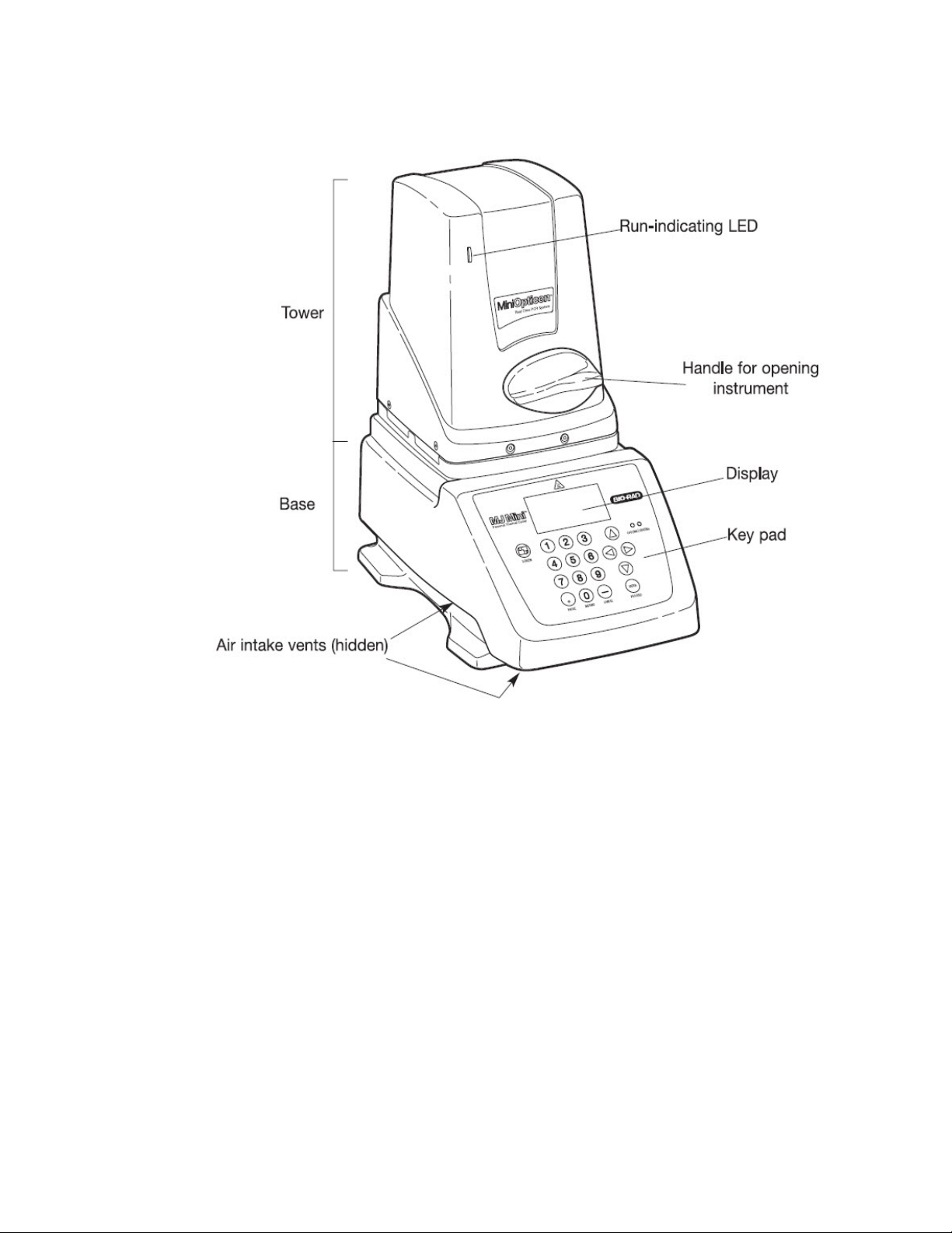
The MiniOpticon system (Figure 1) includes:

• Optical tower. This tower includes an optical system to collect fluorescent data

NOTE: The serial number of the MiniOpticon system is located on a sticker on the back of the optical tower.

System Installation

• MJ Mini™ thermal cycler base. The MiniOpticon system includes a thermal cycler block that rapidly heats and cools samples.

Figure 1. Front view of the MiniOpticon system.

When open, the MiniOpticon system includes these features:

• Inner lid with heater plate. The heater lid maintains temperature on the top of the reaction vessel to prevent sample evaporation. Avoid touching or otherwise contaminating the heater plate. Never poke anything through the holes, the apical system can be damaged.

• Block. Load samples in this block before the run

WARNING! Prevent contamination of the instrument by spills, and never run a

reaction with an open or leaking sample lid. For information about general cleaning and maintenance of the instrument, see “Instrument Maintenance” (page 127).

WARNING! Avoid touching the inner lid or block: These surfaces can be hot.

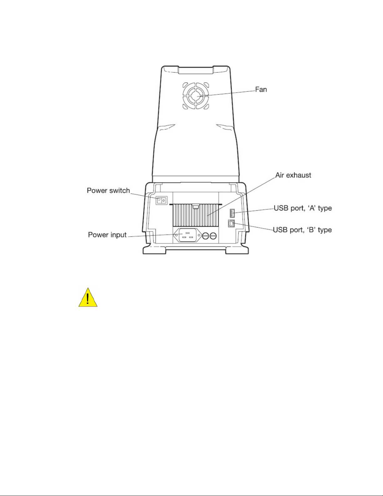
The back panel of the MiniOpticon system includes these features (Figure 2):

• Power switch. Press the power switch to turn the power on

• Power input. Plug in the power cord here

MiniOpticon Instruction Manual

• USB connections. Use these ports to connect the MiniOpticon system to a computer

Figure 2. Back panel of MiniOpticon System.

WARNING! Avoid contact with the back panel during operation.

System Requirements

To operate the MiniOpticon system, use the following power sources and cables:

• Input power. 100—240 VAC, 50—60 Hz

• Indoor use. Ambient temperature of 15—31oC. Relative humidity maximum of 80%

(non-condensing)

• Air Supply. The MiniOpticon system requires a constant supply of air that is 31°C or cooler in order to remove heat from the heat sink. Air is taken in from the lower vents located on the sides and front of the instrument and exhausted from the fan in the back. If the air supply is inadequate or too hot, the instrument can overheat, causing performance problems and even automatic shutdowns

WARNING! Do not place the MiniOpticon system on a lab bench covered by bench paper. The bench paper can prohibit sufficient air circulation.

• USB cable. Control the MiniOpticon system using only the USB cable provided from Bio-Rad. This cable is sufficiently shielded to help prevent data loss

System Installation

Setting Up the system

The MiniOpticon system should be installed on a clean, dry, level surface with sufficient cool airflow to provide adequate air supply to run properly. The MiniOpticon system requires a location with power outlets to accommodate the MiniOpticon system and the computer.

NOTE: Only one MiniOpticon system should be connected to a computer at one time.

Installing the MiniOpticon System

To install the MiniOpticon system:

1. Your MiniOpticon system shipment includes the components listed below. Remove all packing materials and store them for future use. If any items are missing or damaged, contact your local Bio-Rad office.

• MiniOpticon system

• USB cable

• CFX ManagerTM software installation CD

• Instruction manual

• CFX Manager software quick guides for protocol, plate, data analysis, and gene

expression analysis

2. Firmly grasp the instrument from beneath to support the weight of the cycler and the optical tower. Carefully lift the instrument out of the shipping box.

WARNING! Do not lift the instrument by the green handle.

3. Insert the power cord plug into its jack at the back of the instrument.

4. Plug the power cord into a standard 110 V or 220 V electrical outlet. The MiniOpticon system will accept 220 V automatically. Avoid plugging the MiniOpticon system into a power outlet that is already being used for other laboratory equipment

NOTE: Turn the system on only after installing CFX Manager software. The power switch is on the back right-hand side of the MiniOpticon system.

Installing CFX Manager Software

CFX Manager software is run on a personal computer (PC) with either the Windows XP, Windows Vista, or Windows 7 operating system and is required to run and analyze real-time PCR data from the MiniOpticon system. Table 6 lists the computer system requirements for the software.

Table 6. Computer requirements for CFX Manager software.

System Minimum Recommended

Operating system Windows XP Professional SP2 and

above, Windows Vista, or Windows 7 Home Premium and above.

Drive CD-ROM drive CD-RW drive

Hard drive 10 GB 20 GB

Processor speed 2.0 GHz 2.0 GHz

RAM 1 GB RAM (2 GB for Windows

Vista)

Screen resolution 1024 x 768 with true-color mode 1280 x 1024 with true-color mode

Windows XP Professional SP3 or Windows 7.

2 GB RAM

MiniOpticon Instruction Manual

Table 6. Computer requirements for CFX Manager software. (continued)

System Minimum Recommended

USB USB 2.0 Hi-Speed port USB 2.0 Hi-Speed port

WARNING! Running a MiniOpticon system with CFX Manager software on a PC computer with a Windows 64-bit operating system is not supported due to incompatible USB drivers. A PC computer with a 64-bit processor (like Intel) on a 32-bit Windows operating system is supported.

WARNING! CFX Manager software can be installed on the same computer that

already has Opticon MonitorTM version 3.1 installed. There may be conflicts controlling the instrument if both software packages are opened at the same time with the MiniOpticon turned on.

WARNING! If the computer with the CFX Manager software is running a virus scan program, make sure scans are performed when the MiniOpticon system is idle.

To install the CFX Manager software:

1. Log in to the computer with administrative privileges, the software must be installed on the computer by a user with administrative privileges.

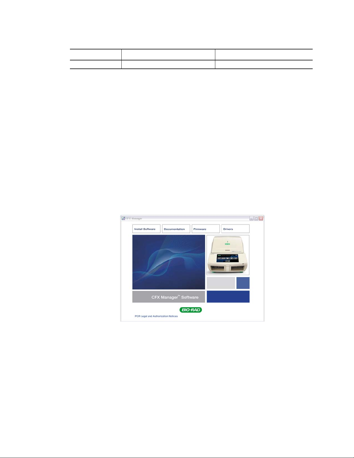
2. Place the CFX Manager software CD in the computer’s CD drive.

3. The software launch page should appear automatically. Double-click Install Software on the software launch page (Figure 3).

Figure 3. Software installation screen.

TIP: Click the Documentation button to find searchable PDF copies of instrument manuals and other documentation.

4. Accept the terms in the license agreement to continue.

5. Follow the instructions on the screen to complete the installation. When completed, the Bio-Rad CFX manager software icon will appear on the desktop of the computer.

System Installation

6. If the launch page does not appear automatically, double-click on (CD drive):\Bio-Rad CFX, then open and follow instructions in the Readme.txt file.

NOTE: For Windows Vista operating system, you will be prompted to install device software for Jungo during the CFX Manager software installation. Click Install to proceed. If prompted with the warning “Windows can’t verify the publisher of this driver software,” Click Install this driver software anyway to proceed.

Installing MiniOpticon System Drivers

The MiniOpticon system drivers must be installed on the computer in order to properly communicate with the device and perform real-time PCR experiments. The drivers are installed automatically during CFX Manager software installation for computers running Windows Vista operating system. Drivers must be installed manually for computers running Windows XP operating system.

NOTE: For Windows XP operating system, three drivers must be installed: Bio-Rad Thermal Cycler (EEPROM Empty), Bio-Rad Mini Optical Module and Bio-Rad Mini Cycler. The driver installation package provides instructions on how to install the drivers correctly.

To install the system drivers for Windows XP:

1. Connect the MiniOpticon system to the computer by plugging a USB cable (square end) into the USB 2.0 port located on the back of the MiniOpticon system, and then connecting the cable (flat end) into the USB 2.0 port located on the computer.

2. Turn the MiniOpticon system on by pressing the switch on the back of the system so that the side marked “I” is depressed.

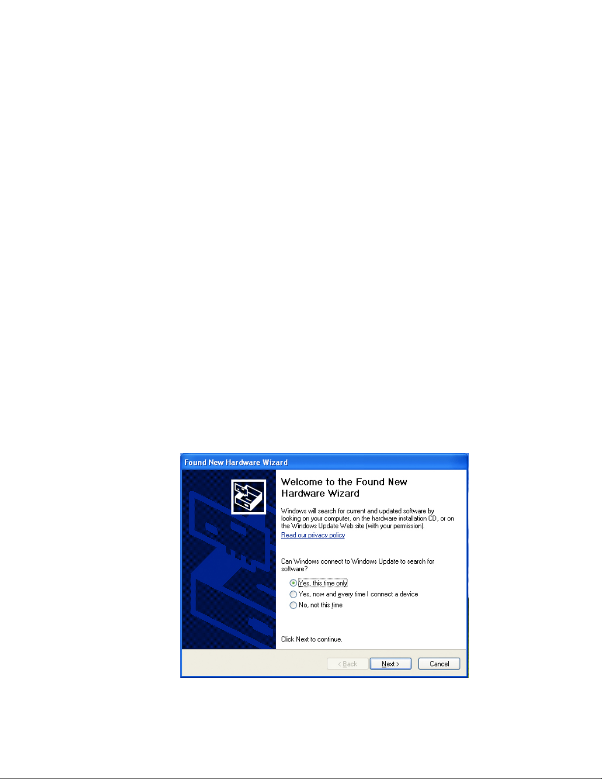
3. Follow the instructions in the Found New Hardware Wizard that launches after the instrument is first detected by the computer.

4. On the first screen, select Yes, this time only to instruct the Windows operating system to connect to Windows Update to search for software (Figure 4). Click Next.

Figure 4. Found New Hardware Wizard.

MiniOpticon Instruction Manual

5. Select Install the software automatically to install the Bio-Rad Thermal Cycler (EEPROM Empty) driver. Click Next (Figure 5).

Figure 5. Software (Driver) installation screen.

6. A window will appear indicating the driver being installed has not passed Windows Logo testing to verify its compatibility with Windows XP. Click Continue Anyway to proceed.

7. Click Finish (Figure 6) at the software installation completion screen when the driver is installed.

Figure 6. Finished Driver installation screen.

8. Repeat the driver installation for the Bio-Rad Mini Optical Module and the Bio-Rad MiniCycler drivers.

System Installation

Running Experiments

Be sure that the MiniOpticon system is connected to the computer and turned on before launching the CFX Manager software. The green protocol-indicator light on the front of the MiniOpticon detector is illuminated only during a protocol run.

WARNING! Remove the shipping plate from the thermal cycler block to operate.

Loading the Block

1. To access the MiniOpticon system’s block, turn the front green handle counter-clockwise until it snaps into the open position. Rotate the entire tower outward, to the left.

2. Place the 48-well, 0.2 ml microplate, or tube strips with sealed lids in the block. Check that the tubes are completely sealed to prevent leakage. For optimal results, load sample volumes of 15–30 µl.

3. To ensure uniform heating and cooling of samples, sample vessels must be in complete contact with the sample holder. Adequate contact is ensured by:

• Verifying the sample holder is clean before loading samples

• Firmly pressing tubes, or a 48-well microplate into the sample holder

TIP: Spin down reactions in tubes or microplates before loading into the thermal cycler block. Air bubbles in samples, or liquid on the plate deck, can affect results.

• Bio-Rad strongly recommends that oil not be used to thermally couple sample

vessels to the block

NOTE: Do not open the MiniOpticon detector while the green protocol-indicator light is illuminated. Opening the door, particularly during a scan of the plate, may interrupt the software’s control of the protocol.

4. To close the instrument, rotate the tower back into the closed position and then turn the green handle clockwise (Figure 1). Both the tower and the handle have spring mechanisms that facilitate closure.

NOTE: For accurate data analysis, check that the orientation of reactions in the block is exactly the same as the orientation of the well contents in the software Plate tab (see “Plate Tab” on page 23). If needed, edit the well contents before, during, or after the run.

WARNING! When running the MiniOpticon system, always balance the tube strips or cut microplates in the wells. For example, if you run one tube strip on the left side of the block, run an empty tube strip (with caps) on the right side of the block to balance the pressure applied by the heated lid.

WARNING! Be sure that nothing is blocking the lid when it closes. Although there is a safety mechanism to prevent the lid from closing if it senses an obstruction, do not place anything in the way of the closing lid.

Recommended Plastic Consumables

Run only white-welled 48-well plates or white-welled strip tubes in the MiniOpticon system. For optimal results, Bio-Rad provides the following consumables for the MiniOpticon system (catalog numbers are provided in bold):

• MLL-4851. Multiplate low-profile 48-well unskirted PCR plates, white color wells

• TLS-0851. Low-profile 8-tube strips, 0.2 ml, without caps, white color wells

• TCS-0803. Optical flat 8-cap strips, for 0.2 ml tubes and plates, ultraclear

MiniOpticon Instruction Manual

2 CFX Manager™ Software

Read this chapter for information about getting started with CFX Manager software.

• Main software window (page 9)

• Startup Wizard (page 12)

• Detected Instruments Pane (page 13)

• Status Bar (page 13)

• Instrument Properties window (page 14)

• Master Mix Calculator (page 15)

• Scheduler (page 16)

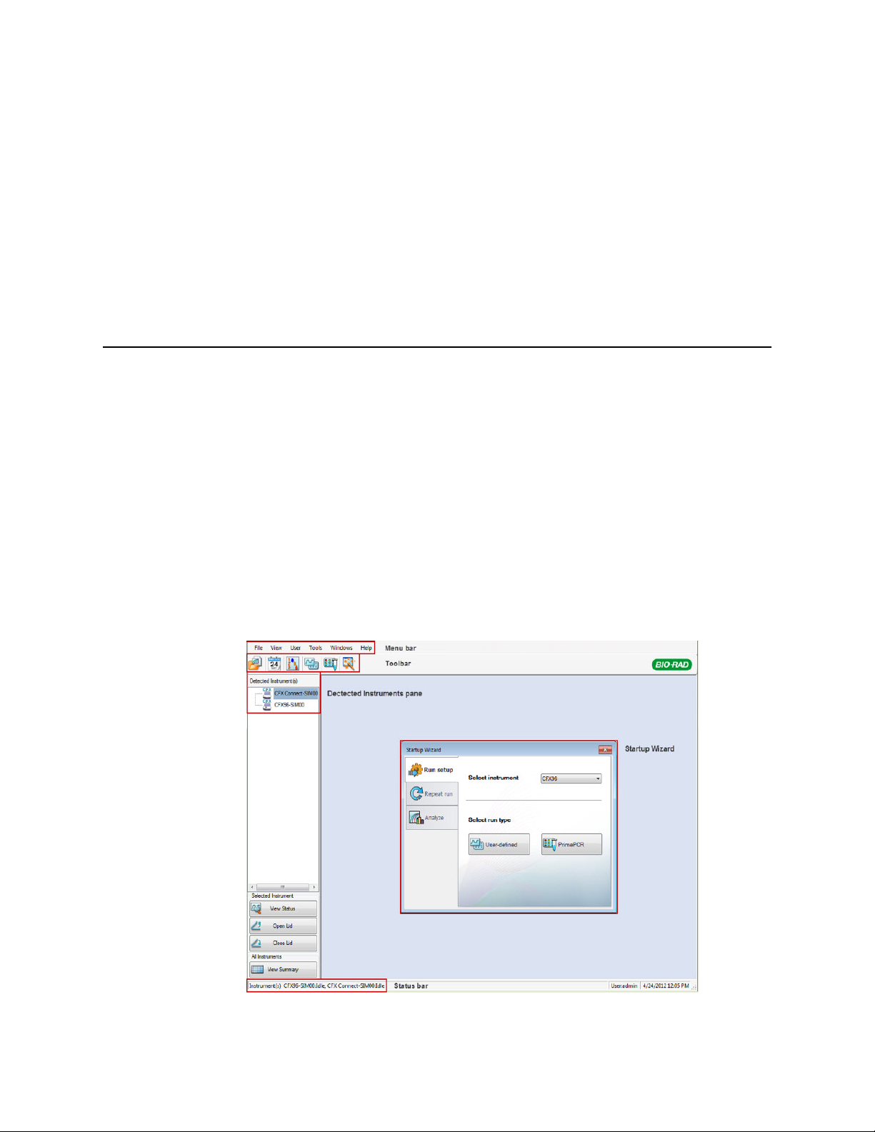
Main Software Window

Features available in the main software window are provided in Figure 7.

Figure 7. The main software window.

CFX Manager™ Software

Menu Bar

The menu bar of the main software window provides the items listed in Table 7.

Table 7. Menu bar items in the main software window

Menu Item Command Function

File New Create a new protocol, plate, run, or Gene Study.

View Application Log Display the application log for the software.

User Select User Open the Select User window to change software

Open Open existing files, including protocol (.prcl), plate

(.pltd), data (.pcrd), Gene Study (.mgxd), and stand-alone run files (.zpcr).

Recent Data Files View a list of the ten most recently viewed data

files, and select one to open in Data Analysis.

Repeat a run Open the Run Setup window with the protocol and

plate from a completed run to quickly repeat the run.

Exit Exit the software program.

Run Reports Select a run report to review from a list.

Startup Wizard Open the Startup Wizard.

Run Setup Open the Run Setup window.

Instrument Summary Open the Instrument Summary window.

Detected Instruments Show or hide the Detected Instruments pane.

Toolbar Show or hide the main software window toolbar.

Status Bar Show or hide the main software window status

bar.

Show Open the Block Status window, application data

folder, user data folder, LIMS file folder, PrimePCR folder, run history, or a window displaying the properties of all connected instruments.

users.

Change Password Change your user password.

User Preferences Open the User Preferences window.

User Administration Manage users in the User Administration window.

MiniOpticon Instruction Manual

Table 7. Menu bar items in the main software window (continued)

Menu Item Command Function

Tools Scheduler Open the Scheduler to make reservations for

instrument use.

Master Mix Calculator Open the Master Mix Preparation calculator.

Protocol AutoWriter Open the Protocol AutoWriter window to create a

new protocol.

Ta Calculator Open the Ta Calculator window to calculate the

annealing temperature of primers.

Dye Calibration Wizard Open the Dye Calibration window to calibrate an

instrument for a new fluorophore.

Reinstall Instrument Drivers

Zip Data and Log Files Choose and condense selected files in a zipped

Options Configure software email settings.

Windows Cascade Arrange software windows on top of each other.

Tile Vertical Arrange software windows from top to bottom.

Tile Horizontal Arrange software windows from right to left.

Close All Close all open software windows.

Help Contents Open the software Help for more information

Index View the index in the software Help.

Search Search the software Help.

qPCR Applications & Technologies Web Site

PCR Reagents Web Site View a website that lists Bio-Rad PCR and real-

PCR Plastic Consumables Web Site

Software Web Site View a website that lists Bio-Rad PCR and real-

Check For Updates Check for software or instrument updates.

About Open a window to see the software version.

Reinstall the drivers that control communication with Bio-Rad real-time PCR systems

file for storage or to email.

about running PCR and real-time PCR.

Open a website to find information about real-time PCR.

time PCR reagents.

View a website that lists Bio-Rad consumables for PCR and real-time PCR runs.

time PCR amplification software.

Toolbar Buttons

Click a button in the toolbar of the main software window (Table 8) for quick access to common software commands.

Table 8. Toolbar buttons in the main software window.

Button Button Name Function

Open a Data File or Gene Study

Open a browser window to locate a data file (*.pcrd extension) and open it in the Data Analysis window or a gene study file (.mgxd extension) open it in the Gene Study window.

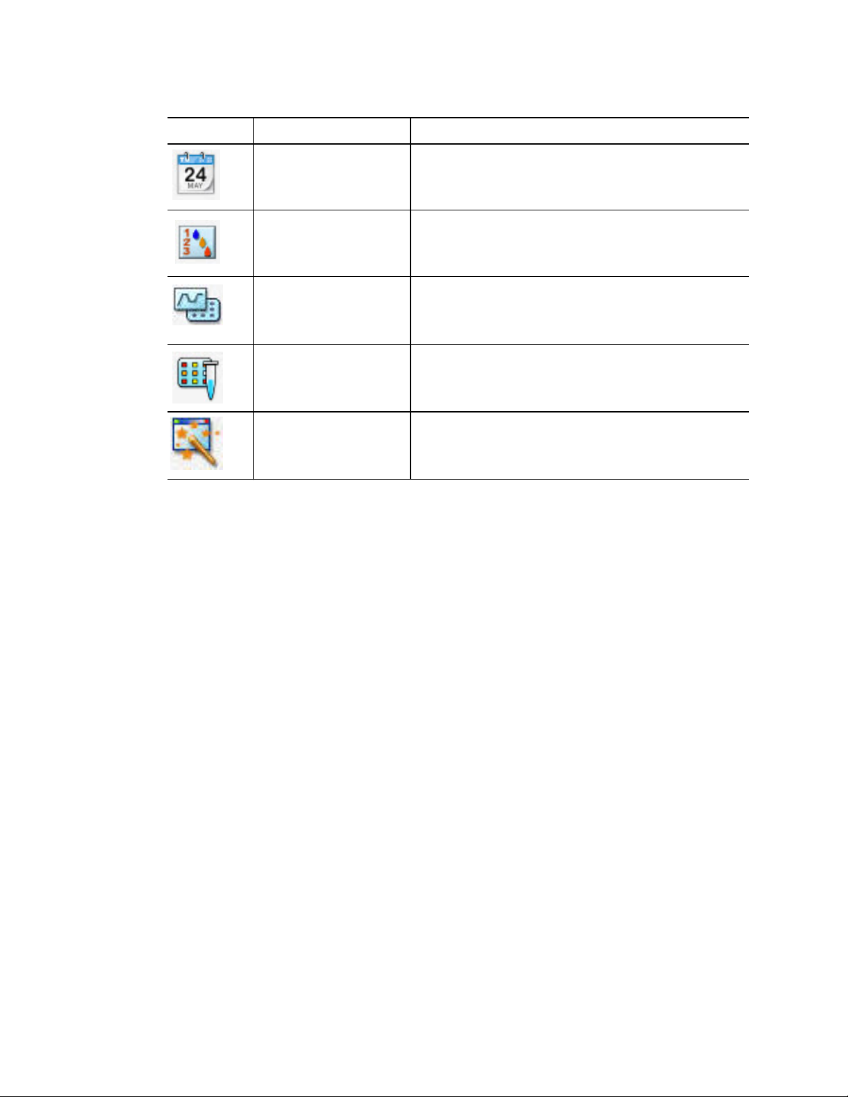
CFX Manager™ Software

Table 8. Toolbar buttons in the main software window. (continued)

Button Button Name Function

Scheduler Open the Scheduler to reserve a PCR instrument.

Master Mix Calculator Open the Master Mix Calculator window to set up

reaction mixes.

User-defined Run Setup Open the Run Setup window to set up a run (page 21).

PrimePCR Run Setup Open the Run Setup window with the default

PrimePCR™ protocol and plate layout loaded based on the instrument selected.

Startup Wizard Open the Startup Wizard that links you to common

software functions (page 12).

Startup Wizard

The Startup Wizard automatically appears when CFX Manager software is first opened. If it is not shown, click the Startup Wizard button on the main software window toolbar.

Options in the Startup Wizard include the following:

• Run setup. Select the appropriate instrument in the pull-down list to ensure the default plate settings match the instrument to be used

• User-defined. Set up the protocol and plate to begin a new run in the Run Setup

window (page 21)

• PrimePCR. Open the Run Setup window with the default PrimePCR protocol and

plate layout (for the selected instrument) loaded. PrimePCR plate layouts are available only for 96- and 384-well plates.

• Repeat Run. Set up a run with the protocol and plate layout from a completed run. If needed, you can edit the run before starting

• Analyze. Open a data file to analyze results from a single run (page 53) or a gene study file for results from multiple gene expression runs (page 97)

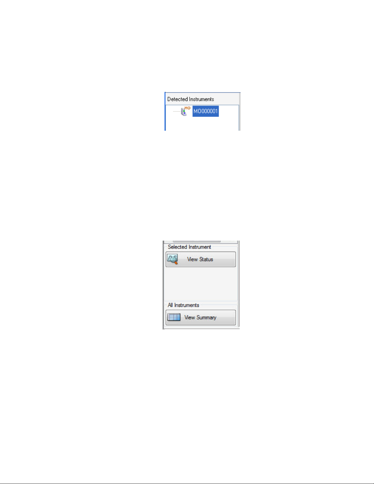
Detected Instruments Pane

The connected instrument appears in the Detected Instruments pane (Figure 8). This list shows each instrument as an icon named with the serial number (default). Right-click on the instrument in the Detected Instruments pane to open the Instrument Properties window and rename the instrument.

Figure 8. Instruments listed in the Detected Instruments pane.

Right-click on the instrument icon to select one of these options:

• View Status. Open the Run Details window to check the status of the selected instrument block

• Flash Block Indicator. Flash the indicator LED on the instrument

• Rename. Change the name of the instrument

• Properties. Open the Instrument Properties window

• Collapse All. Collapse the list of instruments in the Detected Instruments pane

• Expand All. Expand the list of instruments in the Detected Instruments pane

MiniOpticon Instruction Manual

You can also control a block by clicking an instrument block icon in the Detected Instrument pane and then clicking a button in the Selected Instrument pane (Figure 9).

• Click View Status to open the Run Details window to check the status of the

• Click View Summary to open the Instrument Summary window

Status Bar

Figure 9. Buttons at the bottom of the Detected Instrument pane.

selected instrument block

The left side of the status bar at the bottom of the main software window shows the current status of the instruments. View the right side of the status bar to see the current user name, date, and time. Click and drag the right corner of the status bar to resize the main window.

CFX Manager™ Software

Instrument Properties Window

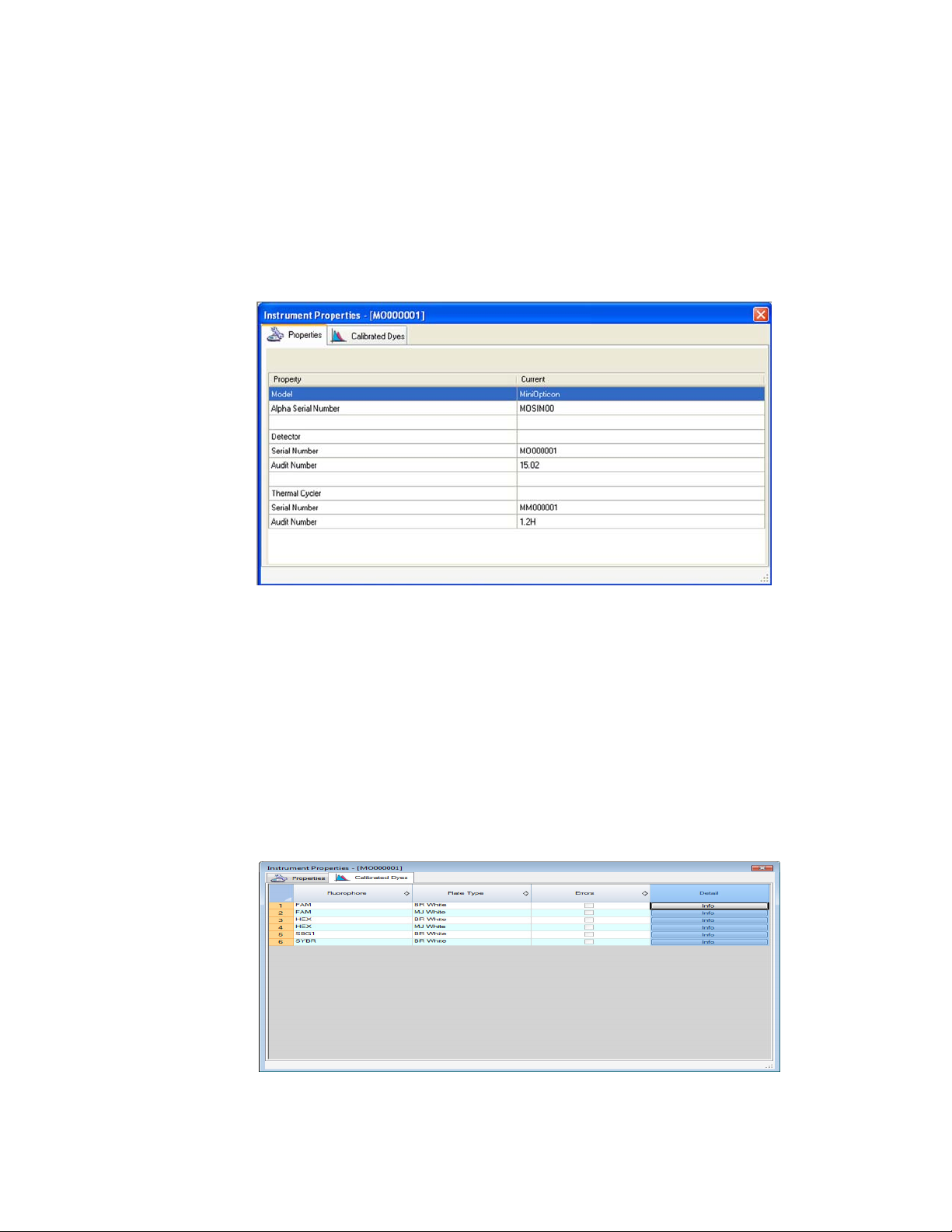
To open the Instrument Properties window to view information about an instrument, right-click on the instrument icon in the Detected Instruments pane (Figure 8). The window includes two tabs (Figure 10):

• Properties. View serial numbers of the MiniOpticon system

• Calibrated Dyes. View the list of calibrated fluorophores

Figure 10. Instrument Properties window.

Properties Tab

The Properties tab displays important serial numbers for the connected instrument. The firmware versions are also displayed. The default name for an instrument is the MiniOpticon serial number, which appears in many locations in the software.

Calibrated Dyes Tab

Open the Calibrated Dyes tab (Figure 11) to view the list of calibrated fluorophores and plates for the selected instrument. Click an Info button to see detailed information about a calibration.

Figure 11. Calibrated Dyes tab in the Instrument Properties window.

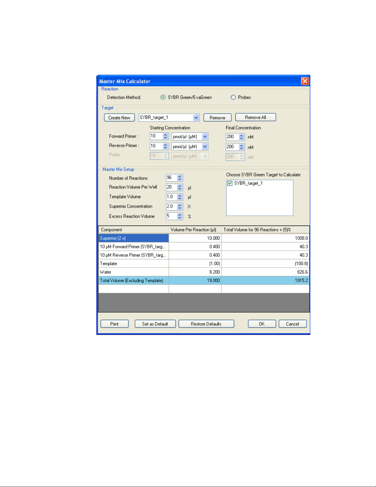
Master Mix Calculator

To open the Master Mix Calculator, click the Master Mix Calculator button in the toolbar (Figure 12) or select Tools > Master Mix Calculator from the main window.

MiniOpticon Instruction Manual

Figure 12. Master Mix Calculator window.

To set up a reaction master mix:

1. Select either SYBR

2. Edit the default target name by highlighting the target name in the dropdown target list, entering a new target name in the Target box and pressing Enter on the keyboard.

3. Enter the starting and final concentrations for your forward and reverse primers and any probes.

4. Additional targets can be added by clicking the New button. To delete targets, select the target using the dropdown target list and click Remove.

Green/EvaGreen or Probes detection method.

CFX Manager™ Software

WARNING! Removing a target from the target list also removes it from any master mixes calculations it is used in.

5. Adjust the Supermix concentration, reaction volume per well, excess reaction volume, the volume of template that will be added to each well, and the number of reactions that will be run.

6. Check the checkbox next to the target (only one can be chosen per SYBR® Green/ EvaGreen master mix) or targets (for probe multiplex reactions). The calculated volumes of the components required for the master mix are listed.

7. To print a master mix calculations table click Print.

8. Click the Set as Default button to set the quantities inputed in the Target and Master Mix Setup sections as new defaults.

9. To save the contents of the Master Mix Calculator window, click OK.

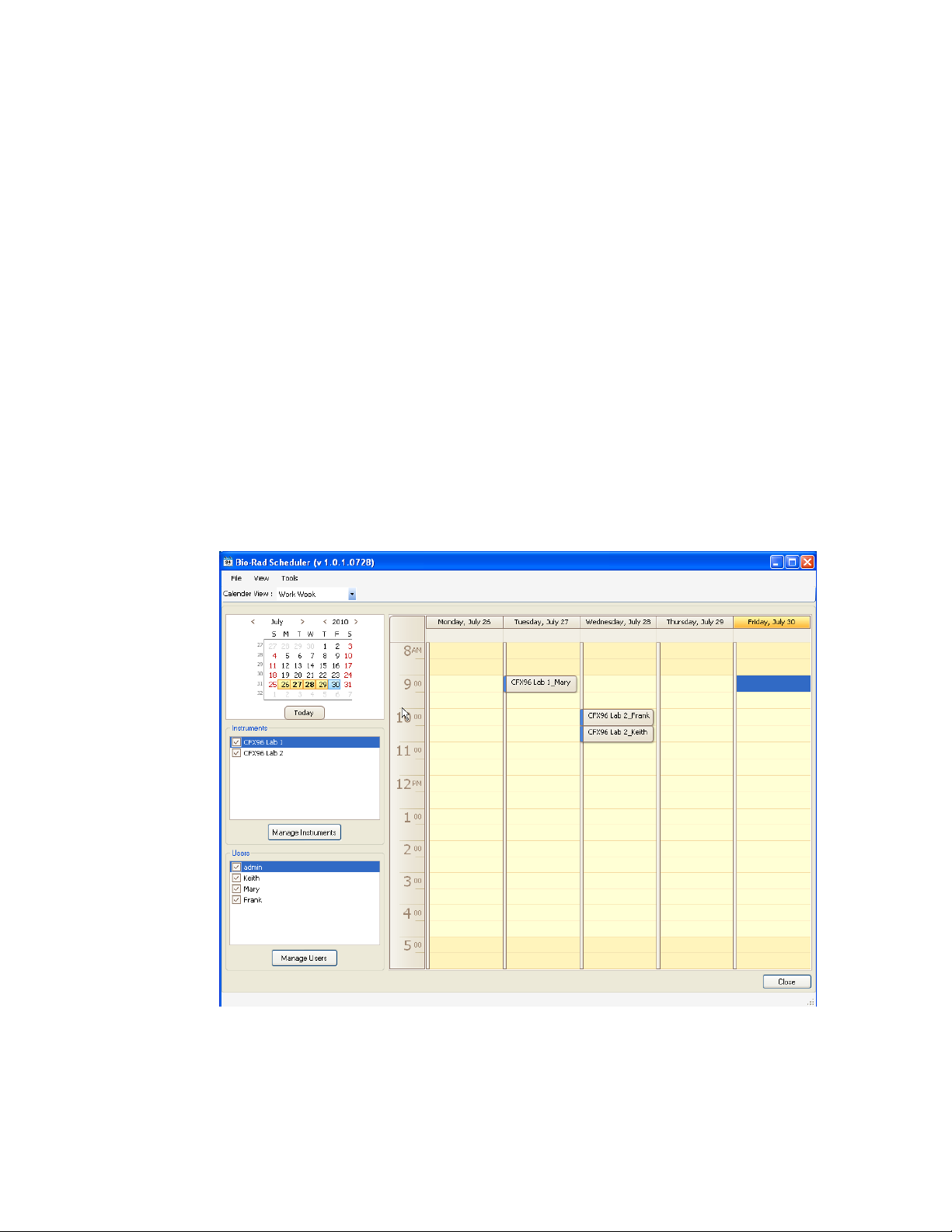
Scheduler

Use the Scheduler to reserve access to an instrument(s). To access the Scheduler click the Scheduler button in the toolbar (Figure 13) or select Tools > Scheduler from the main window.

Figure 13. Scheduler Main Window.

MiniOpticon Instruction Manual

To Set up the Scheduler

1. The first time Scheduler is opened, any User, Instrument, and SMTP email settings will be imported from CFX Manager software.

2. To add a new instrument, select View > Instrument Details or click the Manage Instruments button below the Instruments list (Figure 13) in the scheduler main window. In the Instrument Details window, enter the instrument name in the Name column. Choose a model from the drop down menu or leave it blank to schedule instrument types not listed. Entering base and optical head serial numbers is optional.

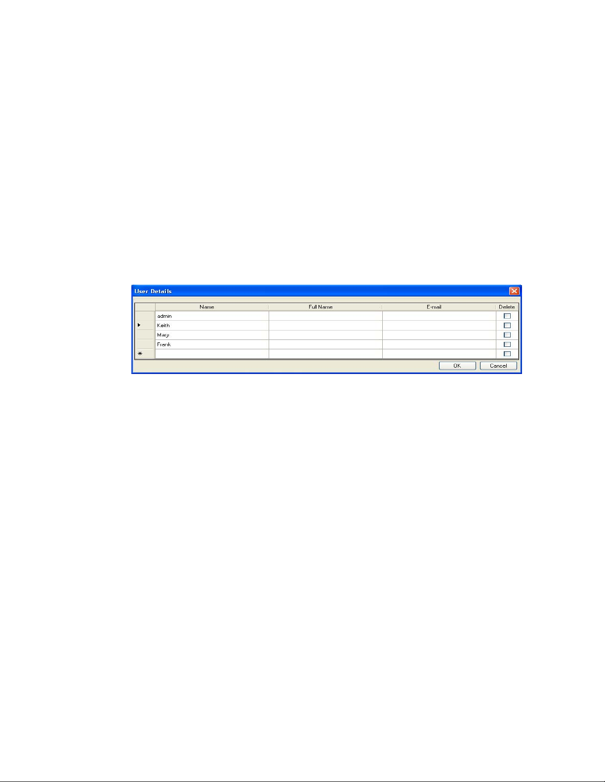
3. To add a new user, select View > User Details or click the Manage Users button below the Users list. In the User Details window (Figure 14), enter the new user name in the Name column. An e-mail address can be entered so that optional electronic notifications can be sent. NOTE: The SMTP server needs to be set up in order for electronic notifications to be enabled.

Figure 14. Scheduler User Details Window.

4. To remove an instrument or user, open the appropriate details window and check the corresponding box in the Delete column.

WARNING! All events associated with this instrument or user will be removed from the calendar.

CFX Manager™ Software

Scheduler Menu Bar

The Scheduler menu bar contents are listed in Table 9.

Table 9. Menu bar items in the Scheduler

Menu Item Command Function

File Print Preview Open the print preview window to adjust print

View Instrument Details Open the instrument details window to view, edit,

Tools Import from CFX

settings.

Print Print the calendar as it appears on the screen.

Exit Exit the scheduler.

add, or delete the name, model, base or optical head serial numbers.

User Details Open the user details window to view, edit, add, or

delete scheduler users.

Log File View the scheduler activity log.

Imports the instruments, users or SMTP e-mail

Manager

Cleanup Events Delete events from the calendar older than the

Options Open a window to specify default calendar

settings from CFX Manager software.

period of time specified in the options window.

settings, create a desktop icon, choose to run the scheduler at start up or define cleanup parameters.

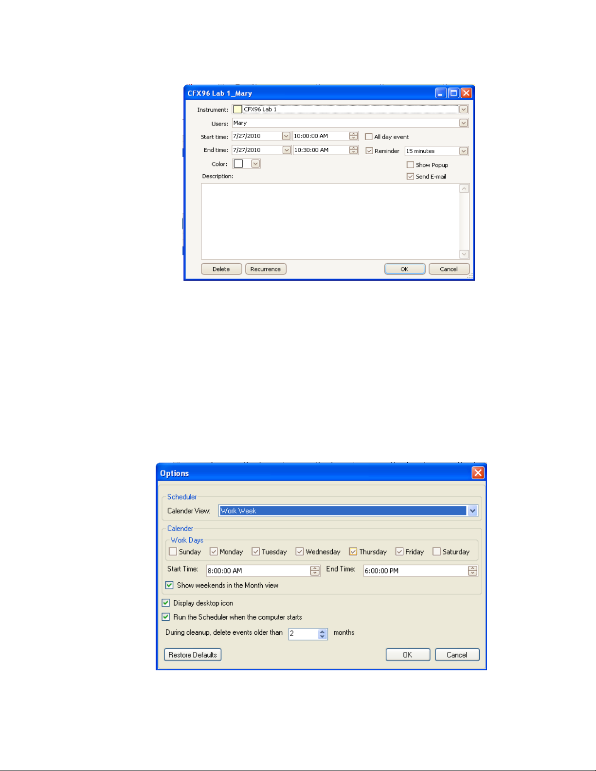
Entering Scheduler Events

To schedule an event:

1. Double click in the appropriate cell in the calendar or right click and choose New Event.

2. Select the instrument and user from the drop down list (Figure 15).

3. Adjust the start and end times. Once an event appears in the calendar view it can be moved to another time period by clicking and dragging the entry to a new position in the calendar.

4. Assign a color to this event (optional).

5. To include an e-mail or a popup reminder that will appear at a specified time prior to the start of an event, check the Reminder check box and choose an advance notification time period for the drop down list.

WARNING! The Scheduler must be running for reminders to be activated. Minimizing the Scheduler window will enable pop-up and e-mail reminders to occur at the scheduled time. Selecting Close will quit the Scheduler.

MiniOpticon Instruction Manual

Figure 15. Scheduler New Event window.

Cleanup events

Select Tools > Cleanup Events to delete events from the calendar older than the period of time specified in the scheduler options window (Figure 16).

WARNING! All events older than the specified date will be deleted.

Scheduler Options

Select Tools > Options to define Scheduler display, cleanup and launch settings. Click Restore Defaults to restore the Scheduler default settings.

Figure 16. Scheduler Options window.

CFX Manager™ Software

MiniOpticon Instruction Manual

3 Performing Runs

Read this chapter for information about performing runs using CFX Manager™ software:

• Run Setup window (page 21)

• Prime PCR™ runs (page 22)

• Protocol tab (page 23)

• End point only runs (page 23)

• Plate tab (page 23)

• Start Run tab (page 24)

• Run Details window (page 25)

• Instrument Summary window (page 28)

Run Setup Window

The Run Setup window provides quick access to the files and settings needed to set up and start a run. To open the Run Setup window, perform one of these options:

• Click the User-defined or the PrimePCR button in the Run Setup tab of the Startup Wizard (page 12)

• Click the User-defined Run Setup or PrimePCR Run Setup button in the main software toolbar (page 9)

• Select File > New > User-defined Run or PrimePCR Run in the main software menu bar (page 10)

The Run Setup window includes three tabs:

• Protocol. Click the Protocol tab to select an existing protocol to run or edit, or to create a new protocol in the Protocol Editor window (page 31)

• Plate. Click the Plate tab to select an existing plate to run or edit, or to create a new plate in the Plate Editor window (page 39)

Performing Runs

• Start Run. Click the Start Run tab (page 24) to check the run settings, select one or

The Run Setup window opens with the Protocol tab in front (Figure 17). To open another tab, click that tab or click the Prev or Next button at the bottom of the window.

more instrument blocks, and begin the run

NOTE: If the protocol currently selected in the Protocol tab does not include a step with a plate read for real-time PCR analysis, then the Plate tab is hidden. To view the Plate tab, add a “Plate Read” (page 33) in at least one step in the protocol.

NOTE: Start a new run from a previous run by selecting File > Repeat a Run in the main software menu bar or Repeat Run in the Startup Wizard. Select the data file (.pcrd) for the run you want to repeat.

Figure 17. Run Setup window, including the Protocol, Plate, and Start Run tabs.

PrimePCR Runs

PrimePCR runs use pathway or disease-specific assays that have been wet-lab validated and optimized and are available from Bio-Rad in the following formats:

• Pre-plated panels. Plates contain assays that are specific for a biological pathway or disease. This option is available only in a 96- or 384-well format

• Custom configured plates. Plates can be set up in a user-defined layout with the option to choose assays for targets of interest, controls, and references. This option is available only in a 96- or 384-well format

• Individual assays. Tubes contain individual primer sets that can be used to manually set up reactions

Select one of the following options to start a PrimePCR run:

• PrimePCR from the Run setup tab on the Startup Wizard

• A PrimePCR run from the Recent Runs list of the Repeat run tab on the Startup Wizard

• File > New > PrimePCR run from the main window

• File > Open > PrimePCR Run File... from the main window

Once a PrimePCR run has been selected, the Run Setup window will open on the Start Run tab with the default PrimePCR protocol and plate layout loaded based on the instrument selected.

To reduce the overall run time, the melt step can be removed by unchecking the box adjacent to Include Melt Step on the Protocol tab. Any other modifications to a PrimePCR run protocol are not recommended since the default protocol was used for assay validation and any deviation from this may affect the results. Changes that are made will be noted in the Run Information tab of the resultant data file and in any reports that are created.

To import target information for PrimePCR plates into a run’s plate layout, select Plate Setup > Apply PrimePCR File from the Real-time Status tab (page 27) or from the Data Analysis window (page 53) and choose the appropriate file (.csv). Select this file by searching in the PrimePCR folder using part of the file name or by browsing to the location on the computer where the file was downloaded from the Bio-Rad website when the plate was ordered.

Protocol Tab

The Protocol tab shows a preview of the selected protocol file loaded in the Run Setup (Figure 17). A protocol file contains the instructions for the instrument temperature steps, as well as instrument options that control the ramp rate and lid temperature.

MiniOpticon Instruction Manual

Select one of the following options to select an existing protocol, create a new protocol, or edit the currently selected protocol:

• Create New button. Open the Protocol Editor to create a new protocol

• Select Existing button. Open a browser window to select and load an existing protocol

• Express Load pull-down menu. Quickly select a protocol to load it into the Protocol tab

• Edit Selected button. Open the currently selected protocol in the Protocol Editor

End Point Only Runs

To run a protocol that contains only an end point data acquisition step, select Options > End Point Only Run from Options in the menu bar of the Run Setup window. The default end point

protocol, which includes two cycles of 60.0°C for 30 seconds, is loaded into the Protocol tab.

To change the step temperature or sample volume for the end point only run, click the Start

Run tab and edit the Step Temperature or Sample Volume.

Plate Tab

The Plate tab shows a preview of the selected plate file loaded in the Run Setup (Figure 18). In a real-time PCR run, the plate file contains a description of the contents of each well, the scan mode, and the plate type. CFX Manager software uses these descriptions for data collection and analysis.

file (.prcl extension) into the Protocol tab

TIP: To add or delete protocols in the Express Load menu, add or delete files (.prcl extension) in the ExpressLoad folder. To locate this folder, select Tools > User Data Folder in the menu bar of the main software window

Select one of the following options to select an existing plate, create a new plate, or edit the currently selected plate:

Performing Runs

• Create New button. Open the Plate Editor to create a new plate

• Select Existing button. Open a browser window to select and load an existing plate file

• Express Load pull-down menu. Quickly select a plate to load it into the Plate tab

• Edit Selected button. Open the currently selected plate in the Plate Editor

(.pltd extension) into the Plate tab

TIP: To add or delete plates in the Express Load menu, add or delete files (.pltd extension) in the ExpressLoad folder. To locate this folder, select Tools > User

Data Folder in the menu bar of the main software window.

Start Run Tab

The Start Run tab (Figure 19) includes a section for checking information about the run that is going to be started and a section for selecting the instrument block.

• Run Information pane. View the selected Protocol file, Plate file, and data acquisition Scan Mode setting. Enter optional notes about the run in the Notes box.

• Start Run on Selected Block(s) pane. Select one or more blocks, edit run parameters (if necessary), and then click the Start Run button to begin the run

Figure 18. Plate tab window.

Figure 19. Start Run tab.

MiniOpticon Instruction Manual

NOTE: You can override the Sample Volume loaded in the Protocol file by selecting the volume in the spreadsheet cell and typing a new volume.

NOTE: A run ID can be entered for each block by selecting the cell and typing an ID or by selecting the cell and scanning with a bar code reader.

To add or remove run parameters from the spreadsheet in the Start Run on Selected Block(s) pane, right-click on the list and select an option in the menu to display. Choose the value to change by clicking the text inside the cell to select it and then typing in the cell, or by selecting a new parameter from the pull-down menu. Editable parameters include:

• Lid Temperature. View the temperature of the lid. Override the lid temperature by selecting the text and typing a new temperature

Run Details Window

When you click the Start Run button, CFX Manager software prompts you to save the name of the data file and then opens the Run Details window. Review the information in this window to monitor the progress of a run.

• Run Status tab. Check the current status of the protocol, open the lid, pause a run, add repeats, skip steps, or stop the run

• Real-time Status tab. View the real-time PCR fluorescence data as they are collected

• Time Status tab. View a full-screen countdown timer for the protocol

Performing Runs

Figure 20 shows the features of the Run Details window.

Figure 20. Run Details window showing the Run Status tab.

Run Status Tab

The Run Status tab (Figure 20) shows the current status of a run in progress in the Run Details window and provides buttons (see below) to control the lid and change the run in progress.

• Run Status pane. Displays the current progress of the protocol.

• Run Status buttons. Click one of the buttons to remotely operate the instrument or to

interrupt the current protocol

• Run Information pane. Displays run details

Run Status Tab Buttons

Click one of the buttons listed in Table 10 to operate the instrument from the software or to change the run that is in progress. NOTE: Changing the protocol during the run, such as adding repeats, does not change the protocol file associated with the run. These actions are recorded in the Run Log.

Table 10. Run Status buttons and their functions

Button Function

This button is disabled for the MiniOpticon™ system.

This button is disabled for the MiniOpticon system.

Add more repeats to the current GOTO step in the protocol. This button is only available when a GOTO step is running.

MiniOpticon Instruction Manual

Table 10. Run Status buttons and their functions (continued)

Button Function

Skip the current step in the protocol. If you skip a GOTO step, the software verifies that you want to skip the entire GOTO loop and proceed to the next step in the protocol.

Flash the run indicating LED on the MiniOpticon system.

Pause the protocol.

NOTE: This action is recorded in the Run Log.

Resume a protocol that was paused.

Stop the run before the protocols ends, which may alter your data.

Real-time Status Tab

The Real-time Status tab (Figure 21) shows real-time PCR data collected at each cycle during the protocol after the first two plate reads. TIP: Click the View/Edit Plate button to open the Plate Editor window. During the run, you can enter more information about the contents of each well in the plate.

Figure 21. The Real-time Status tab displays the data during a run.

Performing Runs

Editing a Plate Setup

The plate setup can be viewed and edited while a run is in progress by selecting the View/Edit Plate button in the Real-Time Status tab. The Plate Editor window will then be presented and

edits can be made as outlined in Chapter 5 (Plates).

The trace styles can also be edited from the Plate Editor window and any changes made will

be visible in the amplification trace plot in the Real-Time Status tab.

Replacing a Plate File

During a run, replace the plate file by selecting Replace Plate file from the Plate Setup dropdown in the Real-time Status tab. The Apply PrimePCR file selection is only applicable to a 96 or 384-well plate.

NOTE: CFX Manager software checks the scan mode and plate size for the plate file; these must match the run settings that were started during the run.

TIP: Replacing a plate file is especially useful if you start a run with a Quick Plate file in the Express Load folder.

NOTE:

Time Status Tab

The Time Status tab shows a countdown timer for the current run.

Instrument Summary Window

The Instrument Summary window (Figure 22) shows a list of the detected instruments and their status. Open the Instrument Summary by clicking the View Summary button (Figure 9 on page 13) in the Detected Instrument pane. Right-click in the Instrument Summary window to change the list of options that appear.

Figure 22. Instrument Summary window.

MiniOpticon Instruction Manual

Instrument Summary Toolbar

The Instrument Summary toolbar includes buttons and functions listed in Table 11.

Table 11. Toolbar buttons in the Instrument Summary window

Button Button Name Function

Set Up Experiment Set up an experiment on the selected

block by opening the Experiment Setup window.

Stop Stop the current run on selected blocks.

Pause Pause the current run on selected blocks.

Resume Resume the run on selected blocks.

Flash Block Indicator Flash the run indicating LED on the

MiniOpticon system.

Open Lid This button is disabled for the

MiniOpticon system.

Close Lid This button is disabled for the

MiniOpticon system.

Hide Selected Blocks Hide the selected blocks in the

Instrument Summary list.

Show All Blocks Show the selected blocks in the

Instrument Summary list.

Show Select which blocks to show in the list.

Select one of the options to show all detected blocks, all idle blocks, all the blocks that are running with the current user, or all running blocks.

Performing Runs

4 Protocols

Read the following chapter for information about creating and editing protocol files:

• Protocol Editor window (page 31)

• Protocol Editor controls (page 33)

• Temperature control mode (page 36)

• Protocol AutoWriter (page 37)

MiniOpticon Instruction Manual

Protocol Editor Window

A protocol instructs the instrument to control the temperature steps, lid temperature, and other instrument options. Open the Protocol Editor window to create a new protocol or to edit the protocol currently selected in the Protocol tab. Once a Protocol is created or edited in the Protocol Editor, click OK to load the protocol file into the Run Setup window and run it.

Opening the Protocol Editor

To open the Protocol Editor, follow one of these options:

• To create a new protocol, select File > New > Protocol or click the Create New button in the Protocol tab (page 22)

• To open an existing protocol, select File > Open > Protocol, or click the Open Existing button in the Protocol tab (page 22)

• To edit the current protocol in the Protocol tab, click the Edit Selected button in the Protocol tab (page 22)

TIP: To change the default settings in the Protocol Editor window, enter the changes in the Protocol tab in the User Preferences window (page 114)

Protocol Editor Window

The Protocol Editor window (Figure 23) includes the following features:

• Menu bar. Select settings for the protocol

• Toolbar. Select options for editing the protocol

• Protocol. View the selected protocol in a graphic (top) and text (bottom) view. Click the

temperature or dwell time in the graphic or text view of any step to enter a new value

Protocols

• Protocol Editor buttons. Edit the protocol by clicking one of the buttons to the left of the text view

Figure 23. Protocol Editor window with buttons for editing protocols.

Protocol Editor Menu Bar

The menu bar in the Protocol Editor window provides the menu items listed in Table 12

Table 12. Protocol Editor menu bar

Menu Item Command Function

File Save Save the current protocol.

Save As Save the current protocol with a new name or in a new

location.

Close Close the Protocol Editor.

Settings Lid Settings Open the Lid Settings window to change or set the Lid

Temperature.

Tools Gradient

Calculator

Run time Calculator

Select the block type for a gradient step. Choose 48 wells for the MiniOpticon system.

Select the instrument and scan mode to be used for calculating the estimated run time in the Experiment Setup window.

MiniOpticon Instruction Manual

Table 13 lists the function of the Protocol Editor toolbar buttons:

Table 13. Protocol Editor toolbar buttons

Toolbar Button and Menus Name Function

Save Save the current protocol file.

Print Print the selected window.

Insert Step Select After or Before to insert steps in a

position relative to the currently highlighted step.

Sample Volume Enter a sample volume in µl between 0 and

50. If you are using higher than 50 µl reactions, select 50 µl. Sample volume determines the Temperature Control mode. Enter zero (0) to select Block mode.

Est. Run Time View an estimated run time based on the

protocol steps and ramp rate.

Help Open the software Help for more

information about protocols.

Protocol Editor Controls

The Protocol Editor window includes buttons for editing the protocol. First, select and highlight a step in the protocol by left clicking it with the mouse. Then click one of the Protocol Editor buttons at the bottom left side of the Protocol Editor window to change the protocol. The location for inserting a new step, “Before” or “After” the currently selected step is determined by the status of the Insert Step box located in the toolbar.

Insert Step Button

To insert a temperature step before or after the currently selected step:

1. Click the Insert Step button.

2. Edit the temperature or hold time by clicking the default value in the graphic or text view, and entering a new value.

3. (Optional) Click the Step Options button to enter an increment or extend option to the step (page 36).

Add or Remove a Plate Read

To add a plate read to a step or to remove a plate read from a step:

1. Select the step by clicking the step in either the graphical or text view.

Protocols

2. Click the Add Plate Read to Step button to add a plate read to the selected step. If the step already contains a plate read, the text on the button changes, so now the same button reads Remove Plate Read. Click to remove a plate read from the selected step.

Insert Gradient Button

To insert a gradient step before or after the currently selected step:

1. Insert a temperature gradient step by clicking the Insert Gradient button.

2. Make sure the plate size for the gradient matches the block type of the instrument. Select the plate size for the gradient by selecting Tools > Gradient Calculator in the Protocol Editor menu bar.

3. Edit the gradient temperature range by clicking the default temperature in the graphic or text view, and entering a new temperature. Alternatively, click the Step Options button to enter the gradient range in the Step Options window (page 36)

4. Edit the hold time by clicking the default time in the graphic or text view, and entering a new time.

Figure 24 shows the inserted gradient step. The temperatures of each row in the gradient are charted on the right side of the window.

Figure 24. Protocol with inserted gradient step.

Insert GOTO Button

To insert a GOTO step before or after the selected step:

1. Click the Insert GOTO button.

MiniOpticon Instruction Manual

2. Edit the GOTO step number or number of GOTO repeats by clicking the default number in the graphic or text view, and entering a new value.

Figure 24 shows an inserted GOTO step at the end of the protocol. Notice that the GOTO loop includes steps 2 through 4.

Insert Melt Curve Button

To insert a melt curve step before or after the selected step:

1. Click the Insert Melt Curve button.

2. Edit the melt temperature range or increment time by clicking the default number in the graphic or text view, and entering a new value. Alternatively, click the Step Options button to enter the gradient range in the Step Options window (page 36).

NOTE: You cannot insert a melt curve step inside a GOTO loop.

NOTE: The melt curve step includes a 30 second hold at the beginning of the step that is not shown in the protocol.

Figure 25 shows a melt curve step added after step 6:

Figure 25. Protocol with inserted melt curve step.

Step Options

To change a step option for the selected step:

1. Select a step by clicking on the step in the graphic or text view.

2. Click the Step Options button to open the Step Options window.

3. Add or remove options by entering a number, editing a number, or clicking a check box.

TIP: To hold a step forever (an infinite hold), enter zero (0.00) for the time.

Protocols

Figure 26 shows the selected step with a gradient of 10oC. Notice that some options are not available in a gradient step. A gradient step cannot include an increment or ramp rate change.

Figure 26. Step option for a gradient.

NOTE: A gradient runs with the lowest temperature in the front of the block (row H) and the highest temperature in the back of the block (row A).

The Step Options window lists the following options you can add or remove from steps:

• Plate Read. Check the box to include a plate read

• Temperature. Enter a target temperature for the selected step

• Gradient. Enter a gradient range for the step

• Increment. Enter a temperature to increment the selected step; the increment amount is

added to the target temperature with each cycle

• Ramp Rate. Enter a rate for the selected step; the range depends on the block size

• Time. Enter a hold time for the selected step

• Extend. Enter a time to extend the selected step. The extend amount is added to the

hold time with each cycle

• Beep. Check the box to include a beep at the end of the step

TIP: When you enter a number that is outside the option range, the software changes the number to the closest entry within the range.

Delete Step Button

To delete a step in the protocol:

1. Select a step in the graphic or text view.

2. Click the Delete Step button to delete the selected step.

WARNING! You cannot undo this function.

Temperature Control Mode

The instrument uses one of two temperature control modes to determine when the sample reaches the target temperature in a protocol.

TIP: The sample volume can be changed before a run by editing the Sample Volume parameter in the Start Run tab (see “Start Run Tab” on page 24).

Enter a sample volume in the protocol editor to select a temperature control mode:

• Calculated mode. When you enter a sample volume between 1 and 50 µl the thermal cycler calculates the sample temperature based on the sample volume. This is the standard mode

• Block mode. When you enter a sample volume of zero (0) µl, the thermal cycler records the sample temperature as the same as the measured block temperature

Protocol AutoWriter

Open the Protocol AutoWriter to quickly write protocols for PCR and real-time PCR runs. To open the Protocol AutoWriter, select one of these options:

• Click the Protocol AutoWriter button in the main software window toolbar

• Select Tools > Protocol AutoWriter from the menu bar in the main software window

Figure 27 shows a protocol (bottom of window) written by the Protocol AutoWriter.

MiniOpticon Instruction Manual

Figure 27. Protocol AutoWriter window with a new protocol.

Creating a Protocol with the Protocol AutoWriter

Follow these steps to use the Protocol AutoWriter to create a new protocol:

1. Click the Protocol AutoWriter button on the toolbar to open the Protocol AutoWriter window.

2. Enter the Annealing Temperature (Ta) and Amplicon Length in the boxes within the Enter Target Values/Enzymes pane. If you do not know the annealing temperature for primers, click the Ta Calculator button to enter the primer sequences and calculate the annealing temperature. For information about the calculations used in the Ta Calculator see Breslauer et al. 1986.

Protocols

3. Select an enzyme type from the list of options (iTaq™, iProof™, or Other).

4. Add parameters in the Additional Parameters (Optional) pane if you want to add a Gradient Range, Hot Start Activation temperature, or Final Extension time in the protocol.

5. Select a protocol speed (Standard, Fast, or Ultrafast) by moving the sliding bar in the Type pane. When you move the sliding bar, the software adjusts the total run time. Select Real-time PCR to tell the software to collect fluorescence data.

6. Review the protocol in the Preview pane and total run time. Make changes as needed.

TIP: Enter the lid temperature and sample volume before each run by editing the parameters in the Start Run tab (see “Start Run Tab” on page 24).

7. Click OK to save the new protocol, or click Cancel to close the window without saving the protocol.

TIP: To edit a protocol written with the Protocol AutoWriter, open the protocol file (.prcl extension) in the Protocol Editor window (page 31).

NOTE: Bio-Rad Laboratories does not guarantee that running a protocol written in the Protocol AutoWriter window will always result in a PCR product.

5 Plates

Read this chapter for information about creating and editing plate files:

• Plate Editor window (page 39)

• Plate size and type (page 42)

• Select Fluorophores window (page 44)

• Well loading controls (page 45)

• Experiment Settings window (page 48)

• Well selector right-click menu items (page 49)

• Well Groups Manager window (page 50)

• Plate Spreadsheet View/Importer window (page 51)

MiniOpticon Instruction Manual

Plate Editor Window

A plate file contains run parameters, such as scan mode and fluorophores, and well contents and instructs the instrument about how to analyze the data. Open the Plate Editor window to create a new plate or to edit the plate currently selected in the Plate tab. Once a plate file is created or edited in the Plate Editor, click OK to load the plate file into the Run Setup window and run it.

To perform a real-time PCR run, you must load the minimal required information in the Plate Editor: at least one well must contain a loaded sample type and fluorophore.

TIP: Change the well contents before, during, and after completion of the run. However, the scan mode and plate size cannot be changed during or after the run.

Opening the Plate Editor

To open the Plate Editor window (Figure 28), follow one of these options:

• To create a new plate, select File > New > Plate or click the Create New button in the Plate tab (page 23)

• To open an existing plate, select File > Open > Plate, or click the Open Existing button in the Plate tab (page 23)

• To edit the current plate in the Plate tab, click the Edit Selected button in the Plate tab (page 23)

• To open the plate associated with a data file, in the Data Analysis window (page 53), click View/Edit Plate on the toolbar

Plates

Figure 28. Plate Editor window.

Plate Editor Menu Bar

The menu bar in the Plate Editor window provides the menu items shown in Table 14.

Table 14. Menu bar items in the Plate Editor.

Menu Item Command Function

File Save Save the plate files.

Save As Save the plate file with a new file name.

Exit Exit the Plate Editor.

View Show Well Notes Select to show this pane in the well loading controls.

Enter notes about one or more wells.

Show Biological Set Name

Plate Loading Guide Show a guide about how to set up a plate and load the

Settings Plate Size Select a plate size that reflects the number of wells in

Select to show this pane in the well loading controls. Select to enter Biological Set names for one or more wells.

wells.

the instrument block. Choose 48 Wells for the MiniOpticon system.

MiniOpticon Instruction Manual

Table 14. Menu bar items in the Plate Editor. (continued)

Menu Item Command Function

Plate Type Choose the type of wells in the plate that holds your

samples. The MiniOpticon system is only factory calibrated for BR White plates. For accurate data analysis, the plate type must be the same as the plate well type used in the experiment. NOTE: You must calibrate new plate types.

Number Convention Select or cancel the selection for Scientific Notation.

Units Select the units to show in the spreadsheets when

performing quantitation of unknowns versus a standard curve.

Editing Tools Setup Wizard Define plate layout and analysis parameters for gene

expression.

Spreadsheet View/ Importer

Flip Plate Flip the plate contents 180 degrees.

View layout or import target/sample information using spreadsheet.

Plate Editor Toolbar

The toolbar in the Plate Editor provides quick access to important plate loading functions.

Table 15 lists the functions available in the Plate Editor toolbar.

Table 15. Plate Editor toolbar buttons.

Toolbar Item Name Function

Save Save the current plate file.

Print Print the selected window.

Zoom Increase or decrease magnification in plate view.

Well Groups Open the Well Groups Manager window and set up well

groups for the current plate.

Trace Styles Select the colors and symbol used for the amplification

traces.

Help Open the software Help for information about plates.

Plates

Table 15. Plate Editor toolbar buttons. (continued)

Toolbar Item Name Function

Plate Loading Guide

Show a quick guide about how to set up a plate and load the wells.

Plate Size and Type

The software applies these plate settings to all the wells during the experiment:

• Plate Size. Select a plate size that represents the size of the reaction module block of your instrument. Choose MiniOpticon from the pull-down menu option on the Startup Wizard to change the default plate size loaded in the Plate tab of the Experiment Settings window. In the Plate Editor, select the plate size from the Settings menu (see Table 14). Plate size cannot be changed during or after the experiment

• Plate Type. For the MiniOpticon system, select the appropriate white wells designation from the Settings menu. For older systems, the plate type MJ White may need to be selected. For new systems, select the plate type BR White. Make sure the fluorophore being used in the experiment is calibrated for the selected plate type

NOTE: The MiniOpticon system is factory calibrated for plates with white wells. Calibration is specific to the instrument, dye, and plate type. To calibrate a new combination of dye and plate type on an instrument, select Tools > Calibration

Wizard (see “Calibration Wizard” on page 126).

Trace Styles

During the plate setup and while a run is in progress, the color of the amplification traces can be modified. These colors will be displayed as the data is being collected, which can be viewed in the Real-time Status window. For more information on Trace Styles, see page 68.

Setup Wizard

The Setup Wizard can be used to enter plate layout information needed for normalized gene expression analysis either before, during or after a run has been completed. Target and sample name and location on plate, reference gene(s), and control sample can all be entered from this window.

The Wizard (Figure 29) can be opened by selecting Editing Tools > Setup Wizard from the Plate Editor window menu bar.

MiniOpticon Instruction Manual

Figure 29. Auto layout tab of Setup Wizard.

Create a plate layout by following these steps:

1. Auto layout tab. Select the area in which samples will be located on the plate by clicking on a well at one edge and then dragging to encompass the area required. Enter the number of targets and samples to be loaded. If the numbers entered do not fit in the area selected, you will need to reduce the numbers or increase the plate area. The orientation of items on the plate and their grouping can be specified.

NOTE: If your plate layout does not have a regular pattern, use the Target names tab to manually position your targets anywhere on the plate. Click and drag to select mulitple wells.

2. Target names tab. Click a target grouping and then enter its name in the box provided. Multiple target groups can be selected by clicking and dragging.

TIP: After entering a name, press Tab to advance to the next grouping on the right or Enter to move to the next group below.

3. Sample names tab. Click a sample grouping and then enter its name in the box provided. Multiple sample groups can be selected by clicking and dragging.

TIP: When entering target or sample names, click and hold the control key to select groups of wells that are not adjacent.

4. Reference targets tab. Click on one or more targets to use as references for normalized gene expression.

5. Control sample tab. Click on one sample to use as a control for relative gene expression calculations.

Plates

6. Click OK to apply the information entered to your plate. Any additional edits can be made using the Plate Editor.

NOTE: Returning to the Auto layout tab will reset the plate layout. The layout can also be reset by selecting Tools > Clear Plate.

TIP: To read text within wells of the plate layout more easily, click the Zoom plate box for a magnified view.

Select Fluorophores Window

The Select Fluorophores window lists fluorophores that can be selected to load into the Plate Editor well loading controls. To open the Select Fluorophores window, click the Select Fluorophores button on the right side of the Plate Editor.

NOTE: You cannot add or remove fluorophores in this list; you must calibrate the new fluorophores on an instrument in the Calibration Wizard (page 126). After calibration, the new fluorophore is added to the Select Fluorophore window.

NOTE: The MiniOpticon system is factory calibrated only for FAM, SYBR HEX. If you intend to use another dye, you must perform a dye calibration. To calibrate a new combination of dye and plate type on an instrument, select Tools > Dye Calibration Wizard (see “Calibration Wizard” on page 126).

and

Click the Selected check box next to the fluorophore name to add or remove the fluorophores to the list on the right side of the Plate Editor window.

In this example, SYBR® is selected from the list of available fluorophores (Figure 30).

Figure 30. Select Fluorophores window.

• Click the Color box next to the fluorophore name and select a new color to represent each fluorophore in the Plate Editor window and Data Analysis charts

NOTE: Before beginning the run, the software verifies that the fluorophores you specified in the plate are calibrated on that instrument. You cannot run a plate if it includes fluorophores that have not been calibrated on that instrument.

Well Loading Controls

A plate file contains information about the contents of each well loaded with sample for a run. After the run, the software links the well contents to the fluorescence data collected during the protocol and applies the appropriate analysis in the Data Analysis window. For example, wells loaded with standard sample type are used to generate a standard curve.

When setting up a gene expression run, consider the following guidelines for well contents:

• Target Name. One or more targets of interest (genes or sequences) in each loaded well. Each target is assigned to one fluorophore

• Sample Name. One identifier or condition that corresponds to the sample in each loaded well, such as “0 hr”, “1 hr”, or “2 hr”

TIP: Target names and sample names must match between wells to compare data in the Gene Expression tab in the Data Analysis window. Each name must contain the same punctuation and spacing. For example, “Actin” is not the same as “actin”, and “2hr” is not the same as “2 hr”. To facilitate consistency in names, enter them in the Target and Sample Names Libraries in the Plate tab in the User Preferences window (page 117).

• Biological Set Name. Select View > Show Biological Set Name to show this pane in the well loading controls and then enter Biological Set names for one or more wells.

MiniOpticon Instruction Manual

Select a well to load contents into by left-clicking in the plate view. Hold down the mouse button and drag to select multiple wells. The buttons and lists on the right side of the plate view include all the options needed to load the wells (Table 16).

Table 16. Options for loading the plate and wells in the Plate Editor.

Option Function

After selecting wells, the Sample Type must be loaded first. Select a Sample Type from the pull-down menu to load it in the selected wells, including Unknown, Standard, NTC (no template control), Positive Control, Negative Control, and NRT (no reverse transcriptase).

Click a Load box to add a fluorophore to the selected wells; each fluorophore corresponds to a target name. To add fluorophores to the Load list, select them in the Select Fluorophores window.

For gene expression analysis or to distinguish among multiple targets, select a name in the Target Name pulldown menu and press the Enter key to load the target name in the well. To delete a target name, select it, press the Delete key, and then press the Enter key.

TIP: To add a new target name to the pull-down menu in the current plate only, type a name in the pull-down box and press the Enter key.

Plates

Table 16. Options for loading the plate and wells in the Plate Editor. (continued)

Option Function

For gene expression analysis or to distinguish among multiple samples, select a Sample Name from the pulldown menu to load that sample name in the selected wells. To delete a sample name, select it in the menu, press the Delete key on your keyboard, and then press Enter.

TIP: To add a new sample name to the pull-down menu in the current plate, type a new name in the pull-down box and press the Enter key.

To load replicate numbers, selected wells must contain identical well contents. If they do not, the software disables this loading control. Click the Load box to add a Replicate # to the selected wells. Click the Clear Replicate # button to clear the replicate number from selected cells.

TIP: To load multiple replicate numbers across a series of wells, click the Replicate Series button.

In the Replicate Series pane you can apply a replicate series to a set of selected wells. Enter the Replicate Group Size by selecting a number that represents the number of samples (wells) in each group of replicates. Select a Starting Replicate # to add replicates.

NOTE: You can load replicate groups with replicate numbers progressing from left to right (Horizontal), or progressing from top to bottom (Vertical).

Enter a concentration to the selected wells with standard sample type by editing or typing a number in the Concentration box. To apply the concentration to one fluorophore in the well, select a single fluorophore from the pull-down menu (<All>) under the concentration box.To delete a concentration, select it, press the Back Space key on your keyboard and then press Enter.

Select multiple wells with a Standard sample type to activate the Dilution Series button.

MiniOpticon Instruction Manual

Table 16. Options for loading the plate and wells in the Plate Editor. (continued)

Option Function

Click the Dilution Series button to enter a dilution series for the concentration of Standard samples, and load a standard curve.

Enter the Starting Concentration for the dilution series, the Replicates from (starting replicate number) and to (ending replicate number), and the Dilution Factor (amount to change the concentration with each replicate group). Select Increasing for a dilution series that increases, or select Decreasing for a dilution series that decreases. Finally, select the fluorophore used for the dilution series from the pull-down menu and click Apply.

Select View> Show Well Notes to show this pane. Enter notes about one or more wells by selecting the wells and typing the notes in the pull-down menu. Any notes you add appear in the spreadsheet on the Quantification Data tab.

Select View > Show Biological Set Name to show this pane. Enter biological set information about one or more wells by selecting the wells and typing a biological set name in the pull-down menu. Entering Biological Set Name information enables sample analysis in one of four configurations defined by the Biological Set Analysis Options. Refer to the Biological Set Analysis Options section for further details.

Click the Experiment Settings button to open the Experiment Settings window to manage the lists of Targets and Samples, and to set up a gene expression run.

Click the Clear Replicate # button to clear the replicates numbers in the selected wells.

Click the Clear Wells button to permanently remove all content in the selected wells.

NOTE: Well contents can also be copied and pasted into other wells. To do this, highlight the well that is to be copied (only one well can be copied at a time), rightclick and select Copy Well. Highlight the wells into which content is be pasted and select Paste Well. Depress and hold the control key to select non-contiguous wells to paste to.

Plates

Experiment Settings Window

To open the Experiment Settings window, perform one of these options:

• In the Plate Editor, click the Experiment Settings button

• While analyzing data in the Data Analysis window, click the Experiment Settings button in the Gene Expression tab

Open the Experiment Settings window to view or change the list of Targets and Samples (Figure 31) or to set the gene expression analysis sample group to be analyzed if Biological

Set Names have been added to the wells.

• Targets. A list of target names for each PCR reaction, such as a genes or sequences of

interest. Click the Reference column to assign reference genes in a run

• Samples. A list of sample names that indicate the source of the target, such as a sample taken at 1 hour (1 hr), or taken from a specific individual (“mouse1”). Click the Control column to assign the control condition for a run

Figure 31 shows the Targets tab with the analysis settings shown.

Figure 31. Targets tab in Experiment Settings window.

Figure 32 shows the Samples Tab with the Analysis Settings shown.

Figure 32. Samples tab in Experiment Settings window.

MiniOpticon Instruction Manual

To adjust the lists in these tabs, use the following functions:

• Add a target or sample name by typing a name in the New box, and clicking Add

• Remove a target or sample name from the list by clicking the Select to Remove box for that row, and then clicking the Remove checked item(s) button

• Select the target as a reference for gene expression data analysis by clicking the box in the Reference column next to the name for that target

• Select the sample as a control sample for gene expression data analysis by clicking the box in the Control column next to the name for that sample

Click the Show Analysis Settings box in the Experiment Settings window to view or change analysis parameters applied in the Gene Expression tab.

To adjust target parameters:

• Click a cell in the Color column to change the color of the targets graphed in the Gene Expression chart

• Enter a number for the efficiency of a target. The software will calculate the relative efficiency for a target using Auto Efficiency if the data for a target includes a standard curve. Alternatively, type a previously determined efficiency

To adjust the settings for a sample in the Samples tab:

• Click a color in the Color column to change the color of the samples graphed in the Gene Expression chart

• Click a box in the Show Graph column to show the sample in the Gene Expression chart using a color selected in the Color column

Well Selector Right-Click Menu Items

Right-click any well to select the items listed in the table below.

Table 17. Right-click menu items in the Plate Editor Well Selector window

Item Function

Copy Well Copy the well contents, which can then be pasted into another

well or wells.

Paste Well Paste the contents from a copied well into another well or

wells.

Copy to Clipboard Copy the text from a well to a clipboard that can then be

pasted into a document.

Copy as Image Copy the well selector view as an image.

Print... Print the well selector view.

Print Selection... Print the current selection.

Export to Excel... Export the data to an Excel spreadsheet.

Export to Text... Export the data as a text document.

Export to Xml... Export the data as a .xml document.

Export to Html... Export the data as a .html document.

Find Search for specific text.

Export Well Info to Excel Export the well text information as a .xml document.

Plates

Well Groups Manager Window

Well groups divide a single plate into subsets of wells that can be analyzed independently in the Data Analysis window. Once well groups are set up, select one in the Data Analysis window to analyze the data as an independent group. For example, set up well groups to analyze multiple experiments run in one plate, or to analyze each well group with a different standard curve.

NOTE: The default well group is All Wells.

Create Well Groups

To create well groups in the Well Groups Manager window, follow these instructions:

1. Click the Well Groups button in the Plate Editor toolbar or click the Manage Well Groups button in the Data Analysis window toolbar.

2. Click Add to create a new group. The pull-down menu shows the group name as Group 1 for the first group.

3. Select the wells that will compose the well group in the plate view by clicking and dragging across the group of wells. Selected wells turn blue in color (Figure 33).

4. (Optional) Change the name of the group by selecting the group name in the pull-down menu and typing a new name.

5. (Optional) Create more well groups by repeating steps 1 and 2.

6. (Optional) Delete well groups by selecting the group name in the pull-down list, and clicking the Delete button.

7. Click OK to finish and close the window, or click Cancel to close the window without making changes.

Figure 33. Color of wells in the Well Group Manager window.

Plate Spreadsheet View/Importer Window

The Plate Spreadsheet View window shows the contents of a plate in the Plate Editor. Open the Plate Spreadsheet View window (Figure 34) by selecting Editing Tools > Spreadsheet View/Importer in the Plate Editor menu bar.

MiniOpticon Instruction Manual

Figure 34. Plate Spreadsheet View window.

Open the spreadsheet view to import or export the well contents to Excel or to another tabdelimited format:

• Click Export Template to export a plate spreadsheet template to an Excel file (.csv format). This template may be edited and used for import of well content information.

• Click Import to import well contents from a comma delimited file

• Sort or edit a column by selecting it and using these methods:

• Sort the spreadsheet according to the data in one column by clicking the diamond

next to a column name

• Edit the contents of a column that has an asterisk (*) at top by clicking and typing

in each well

NOTE: Select the units for the standard curve data in the Quantity column by opening the Plate Editor and selecting Settings > Units in the menu bar. After the plate runs, the data from these standards appear in the Standard Curve chart of the Quantification tab (Data Analysis window) with the units you select.

Right-click on the spreadsheet to select one of these options from the right-click menu:

• Copy. Copy the entire spreadsheet

• Copy as Image. Copy the spreadsheet as an image file

• Print. Print the spreadsheet

• Print Selection. Print only the selected cells

• Export to Excel. Export the file as an Excel- formatted file

• Export to Text. Export the file as a text file

• Export to Xml. Export the file as a .xml file.

• Export to Html. Export the file as a .html file.

• Find. Find text in the spreadsheet

• Sort. Sort the spreadsheet by selecting up to three columns of data in the Sort window.

Plates

MiniOpticon Instruction Manual

6 Data Analysis Overview

Read this chapter for information about data analysis:

• Data Analysis window (page 53)

• Quantification tab (page 56)

• Well groups (page 57)

• Data analysis settings (page 58)

• Well selectors (page 61)

• Charts (page 63)

• Spreadsheets (page 64)

• Export (page 65)

Data Analysis Window

During data analysis, changing the way the data are displayed by changing the contents of the wells in the Plate Editor never changes the fluorescence data that were collected from each well during the run. Once the module collects fluorescence data, you cannot delete those data but you can choose to remove data from view and analysis.

To change the content of wells after a run, select one of the following options from the Plate Setup button at the top of the Data Analysis window:

• Edit/View Plate. Open the Plate Editor to make manual changes to the layout

• Replace Plate file. Select a previously saved plate file to replace the current plate layout

• Apply PrimePCR file. PrimePCR™ files are not be available for 48-well plates

CFX Manager™ software processes real-time PCR data automatically at the end of each run, and opens the Data Analysis window to display these data. Choose one of these methods to open existing data files in the Data Analysis window:

• Drag a data file (.pcrd extension) over the main software window and release it

• Select Analyze tab in the Startup Wizard window and either select from Recent Files or click the Browse button to find

• Select File > Open > Data File in the main software window to select a file in the Windows browser

• Click the Data Analysis button in the main software window toolbar to select a file in the Windows browser

Data Analysis Overview

• Select File > Recent Data Files to select from a list of the ten most recently opened data files

The Data Analysis window displays multiple tabs (Figure 35), each tab showing the analyzed data for a specific analysis method or run-specific information. Tabs will only be displayed if the data collected in the run are available for that type of analysis.

TIP: To choose the tabs displayed, select View in the main windown. To return to the original tab layout, select Settings > Restore Default Window Layout.

Data Analysis Toolbar

The toolbar in the Data Analysis window (Figure 36) provides quick access to important data analysis functions.

Figure 35. Data Analysis window tabs.

Figure 36. Toolbar in the Data Analysis window.

Table 18 lists the functions of buttons in the toolbar.

Table 18. Toolbar in the Data Analysis window.

Toolbar Button Name Function

Plate Setup View/Edit plate: Open the Plate Editor to view and edit

the contents of the wells. Replace Plate file: Select a plate file to replace the plate layout. Apply PrimePCR file: Select a run file to replace the plate layout for a PrimePCR run.

Manage Well Groups

Well Group Select an existing well group name from the pull-down

Analysis Mode Select to analyze the data in either Fluorophore or

Help Open the software Help for more information about

Open the Well Groups Manager window to create, edit and delete well groups.

menu. The default selection is All Wells. This will only be displayed if well groups have been created.

Target mode.

data analysis.

MiniOpticon Instruction Manual

Data Analysis Menu Bar

The menu bar in the Data Analysis window provides these menu items.

Table 19 lists the functions of items in the menu bar.

Table 19. Right-click menu items for spreadsheets.

Menu Item Command Function

File Save Save the file.

Save As Save the file with a new name.

Repeat Run Extract the protocol and plate file from the

current run to rerun it.

Exit Exit the Data Analysis window.

View Run Log Open a Run Log window to view the run

log of those data file.

Quantification, Melt Curve, Gene Expression, End Point, Custom Data View, QC, Run Information

Settings Cq Determination Mode Select Regression or Single Threshold

Baseline Setting Select Baseline Subtraction method for

Analysis Mode Select to analyze data by Fluorophore or

Cycles to Analyze Select the cycles that are to be analyzed.

Baseline Thresholds Open the Baseline Thresholds window to

Trace Styles Open the Trace Styles window.

Plate Setup Open the Plate Editor to view and edit the

Include All Excluded Wells All excluded wells are included in the

Mouse Highlighting Turn on or off the simultaneous

Select the tabs displayed in the Data Analysis window. At least one tab must be selected.

mode to determine how Cq values are calculated for each trace.

the selected well groups.

by Target.

adjust the baseline or the threshold.

plate; replace the current plate with one from a user-defined plate file or a PrimePCR run file.

analysis.

highlighting of data with the mouse pointer.

TIP: If the Mouse Highlighting is turned off, then hold down the Control key to temporarily turn on the highlighting.

Restore Default Window Layout Restores the arrangement of windows to

the default setting.

Export Export All Data Sheets to Excel Export all the spreadsheet views from

every tab to a separate Excel formatted file.

Export RDML File Open a Save As window to specify an

RDML file name and location.

Data Analysis Overview

Table 19. Right-click menu items for spreadsheets. (continued)

Menu Item Command Function

Custom Export... Open the Custom Export window in which

Export to LIMS Folder... Open a window to save data in a pre-

Tools Reports... Open the Report for this data file.

Well Group Reports... Open the Well Group Report window to

Import Fluorophore Calibration...

Quantification Tab

Each tab in the Data Analysis window displays data in charts and spreadsheets for a specific analysis method and includes a well selector to select the data you want to show. The Data Analysis window opens with the Quantification tab (Figure 37) in front. The Amplification chart data in this tab should be used to determine the appropriate analysis settings for the run.

the fields to be exported and the file format can be specified.

determined format to the LIMS folder.

generate reports for specified well groups.

Select a calibration file to apply to the current data file.

Figure 37. Layout for the Quantification tab in the Data Analysis window.

NOTE: The software links the data in the panes of each Data Analysis tab. For example, highlighting a well by placing the mouse pointer over the well in the well selector view highlights the data in all the other panes.

MiniOpticon Instruction Manual

Step Number Selector

The MiniOpticon™ system can acquire fluorescence data at multiple protocol steps; the software maintains the data acquired at each step independently. The software displays the Step Number selector below the Standard Curve chart on the Quantification tab whenever a protocol contains more than one data collection step. When you select a step, the software applies that selection to all the data that are shown in the Data Analysis window. Figure 38 shows the data collection step number is 3 for all the data.

Figure 38. Step Number selection in the Data Analysis window.

Viewing Well Groups in Data Analysis

Wells in the plate can be grouped into subsets for independent analysis using well groups. When you create well groups in the Well Groups Manager window (page 50), group names appear in the Data Analysis window Well Groups drop-down list on the toolbar.

TIP: To edit, create and delete well groups, click the Manage Well Groups button in the toolbar.

By default, the well group All Wells is selected when the Data Analysis Window is first opened, with the data in all wells with content shown in the charts and spreadsheets.

Figure 39 shows Group 2 selected in the Well Groups menu. Only the wells in that well group appear loaded with content in the well selector and data only for these wells are included in the data analysis calculations.

Figure 39. Data Analysis window with Group 2 selected.

Data Analysis Overview

Data Analysis Settings

The Amplification chart data in the Quantification tab shows the relative fluorescence (RFU) for each well at every cycle. Each trace in the chart represents data from a single fluorophore in one well. These data are used to determine Cq values for each well on a per fluorophore

basis. The software uses one of two modes to determine C

• Regression. This mode applies a multivariable, nonlinear regression model to individual

well traces and then uses this model to compute an optimal Cq value

• Single Threshold. This mode uses a single threshold value to calculate the Cqvalue based on the threshold crossing point of individual fluorescence traces

Select Settings > Cq Determination Mode to choose the Cq determination mode.

Adjusting the Threshold

In Single-Threshold mode, adjust the threshold for a fluorophore by clicking on the threshold line in the Amplification chart and moving the mouse pointer vertically. Alternatively, specify an exact crossing threshold for the selected fluorophore by following these instructions:

1. Select one fluorophore in the fluorophore selector in the Quantification tab (Figure 37) by clicking the boxes next to the fluorophore name located under the Amplification chart.

values:

2. Select Settings > Baseline Thresholds in the menu bar to open the Baseline Thresholds window.

3. Adjust the crossing threshold (Figure 40) for the fluorophore by clicking User Defined and entering a threshold number.

Figure 40. Baseline Thresholds window.

4. Click OK to confirm the change and close the window.

TIP: To have the same threshold value used for all of your data files define this in the Data Analysis tab of the User Preferences window. This value will be applied to all subsequently created data files.

MiniOpticon Instruction Manual

Baseline Settings

The software automatically sets the baseline individually for each well. Select the Baseline Setting to determine the method of baseline subtraction for all fluorescence traces. Select

Settings > Baseline Setting to choose one of these three options:

• No Baseline Subtraction. The software displays the data as relative fluorescence

traces. Some analysis is not possible in this analysis mode, and therefore the software does not display the Gene Expression, End Point, and Allelic Discrimination tabs

• Baseline Subtracted. The software displays the data as baseline subtracted traces for each fluorophore in a well. The software must baseline subtract the data to determine quantification cycles, construct standard curves, and determine the concentration of unknown samples. To generate a baseline subtracted trace, the software fits the best straight line through the recorded fluorescence of each well during the baseline cycles, and then subtracts the best fit data from the background subtracted data at each cycle

• Baseline Subtracted Curve Fit. The software displays the data as baseline subtracted traces, and the software smoothes the baseline subtracted curve using a centered mean filter. This process is performed so that each C

Along with the options above, the following can also be selected:

• Apply Fluorescent Drift Correction. For wells that have abnormally drifting RFU values during the initial few cycles of a run the software derives an estimated baseline from adjacent wells for which a horizontal baseline was successfully generated

is left invariant

Adjusting the Baseline

Once wells for analysis have been selected, check the baseline settings in these wells. Open the Baseline Thresholds window (Figure 40) to change the default baseline for selected wells. To open this window:

1. Select a single fluorophore in the Quantification tab (Figure 37) by clicking the boxes next to the fluorophore name located under the Amplification chart.

2. Select Settings > Baseline Threshold to open the Baseline Threshold window.

To adjust the begin and end baseline cycle for each well:

1. In the Baseline Cycles pane, select one or more wells by clicking the row number, clicking the top left corner to select all wells, holding down the Control key to select multiple individual wells, or holding down the shift key to select multiple wells in a row.

2. Adjust the Baseline Begin cycle and Baseline End cycle for all selected wells or change the Begin and End cycle number at the bottom of the spreadsheet (Figure 40).

3. To revert the settings back to the last saved values, click Reset All User Defined Values.

4. Click OK to confirm any changes and close the window.

Analysis Mode

Data can be analyzed and displayed grouped by either fluorophore or target name. To choose the data analysis mode, select Settings > Analysis Mode or make a selection from the Analysis Mode drop down menu in the toolbar.

Data Analysis Overview

When Fluorophore is chosen data traces are displayed by fluorophore as indicated in the plate setup for that run. Individual fluorophore data is displayed in the amplification and standard curve chart (if available) by checking the appropriate fluorophore selector check boxes located below the amplification chart (Figure 41).

Figure 41. Fluorophore analysis mode selected.

When Target is selected data traces are displayed by target name as entered in the plate setup.

Figure 42. Target analysis mode selected.

Cycles to Analyze

To restrict data analysis to a specified range of cycles, select Settings > Cycles to Analyze. Select the starting cycle and the ending cycle using the arrow buttons or by typing in the desired values and pressing Enter. Click the Restore Defaults button to return to the cycles originally used for analysis.

NOTE: Removing cycles from the beginning of a run can have a significant impact on baselining.

Well Selectors

Click the wells in the well selector to show or to hide the data in the charts or spreadsheets throughout the Data Analysis window:

• To hide one well, highlight and click the individual well. To show that well, highlight and click the well again

• To hide multiple wells, click and drag across the wells you want to select. To show those wells, click and drag across the wells again

• Click the top left corner of the plate to hide all the wells. Click the top left corner again to show all wells

• Click the start of a column or row to hide those wells. Click the column or row again to show the wells

MiniOpticon Instruction Manual

Only wells loaded with content (entered in the Plate Editor) can be selected in the well selector, and their color shows if they are selected. As shown in Figure 43, the well selector shows these three types of wells:

• Selected, loaded wells (blue). These wells contain a loaded Unk (unknown) sample type. The data from these wells appear in the Data Analysis window

• Unselected, loaded wells (light gray). These wells contain loaded Std and Pos sample types. The data from unselected wells do not appear in the Data Analysis window

• Empty wells (dark gray). These wells were not loaded in the Plate Editor window

Figure 43. Three well colors appear in a well selector.

Data Analysis Overview

Well Selector Right-Click Menu Items

Right-click on well(s) in the well selector view to select the items listed in Table 20.

Table 20. Right-click menu items in the well selectors

Item Function

Well XX View only this well, remove this well from view, set color for

Selected Wells (right-click and drag)

Copy Copy the content of the well to a clipboard, including Sample

Copy as Image Copy the well selector view as an image.

Print... Print the well selector view.

Print Selection... Print the current selection.

Export to Excel... Export the data to an Excel spreadsheet.

Export to Text... Export the data as a text document.

Export to Xml... Export the data as a .xml document.

Well Labels Change the well labels to Sample Type, Target Name or

this well, or exclude this well from analysis.

View only these wells, remove these wells from view, set color for these wells, or exclude these wells from analysis.

Type and optional Replicate #.

Sample Name.

Temporarily Exclude Wells from Analysis

USING RIGHT-CLICK

1. To exclude a single well, right-click on the well in the well selector, on a fluroescence trace, or on a point plotted on the standard curve, select Well XX > Exclude from Analysis (Figure 44).

2. To exclude multiple wells, right click and drag to highlight multiple wells, traces or points, click on Selected Wells > Exclude from Analysis.

Figure 44. Right-click to exclude a well from analysis.

NOTE: To re-include an excluded well, click on the appropriate well in the well selector, right click and select Include Well XX in Analysis.

MiniOpticon Instruction Manual

USING THE PLATE EDITOR

1. Click the Plate Setup button on the toolbar in the Data Analysis window.

2. Clicks View/Edit Plate...

3. Select one or more wells in the well selector view.

4. Click Exclude Wells in Analysis (Figure 45) to exclude the selected wells. This checkbox is at the bottom of the Plate Editor controls on the right side of the window.

Charts

Figure 45. Exclude Wells in Analysis Checkbox at bottom of the pane.

5. The excluded well(s) are marked with an asterisk (*) in the Plate Editor window.

Alternatively, to permanently remove wells from analysis, clear the contents from wells in the Plate Editor by clicking the Clear Wells button.

WARNING! You will have to reenter any well content that is cleared.

Each chart in the Data Analysis window displays the data in a different graph and includes options for adjusting the data. To magnify an area of the chart, select an area by clicking and dragging the mouse. The software resizes the chart and centers it on the selected area.

TIP: Return the chart to a full view by right-clicking on the chart and selecting Set

Scale to Default from the right-click menu.

Common Right-Click Menu Items for Charts

Right-click menu items are available on all charts. Some of the available items are present for all charts, and these items can be used to change how the data are displayed or to easily export the data from a chart (Table 21)

Table 21. Right-click menu items for charts

Item Function

Copy Copy the chart into the clipboard.

Save Image As... Save the chart image in the selected image file type. Select

from these formats: PNG (default), GIF, JPG, TIF, or BMP.

Data Analysis Overview

Table 21. Right-click menu items for charts (continued)

Item Function

Page Setup... Preview and select page setup for printing.

Print... Print the chart.

Show Point Values Show the point values when the mouse moves over a point

Set Scale to Default Return to the default chart view after magnifying the chart.

Chart Options... Open the Chart Options window to change the chart,

Charts can be copied into Microsoft Word or PowerPoint documents by clicking on the icon in the upper right corner of the pane, dragging, and then releasing at the required location. The image resolution will correspond to that of the screen from which the image was obtained.

NOTE: Menu items that apply to specific charts are described in the next chapter “Data Analysis Overview” (page 53).

Spreadsheets

on the chart.

including changing the title, selecting limits for the x and y axes, showing grid lines, and showing minor ticks in the axes.

The spreadsheets shown in Data Analysis include options for sorting and transferring the data. Sort the columns by one of these methods:

• Click and drag a column to a new location in the selected table

• Click the column header to sort the data in Ascending or Descending order

To sort up to three columns of data in the Sort window, follow these steps:

1. Right-click on the spreadsheet to open the menu and select Sort.

2. In the Sort window, select the first column title to sort. Sort the data in Ascending or Descending order.

3. Select more than one column title by selecting the title in the pull-down menu. Select Ascending or Descending to sort the column in that order.

4. Click OK to sort the data, or click Cancel to stop sorting.

Highlight the data on the associated charts and well selector by holding the mouse pointer over a cell. If you click in the cell, you can copy the contents to paste into another software program.

Common Right-Click Menu Items for Spreadsheets

Right-click any spreadsheet view to select the items shown in Table 22.

Table 22. Right-click menu items for spreadsheets.

Item Function

Copy Copy the contents of the selected wells to a clipboard,

then, paste the contents into a spreadsheet such as Excel.

Copy as Image Copy the spreadsheet view as an image file and paste it

into a file that accepts an image file such as text, image, or spreadsheet files.

Export

MiniOpticon Instruction Manual

Table 22. Right-click menu items for spreadsheets. (continued)

Item Function

Print... Print the current view.

Print Selection... Print the current selection.

Export to Excel... Export the data to an Excel spreadsheet.

Export to Text... Export the data to a text editor.

Export to Xml... Export the data to an Xml file.

Export to Html... Export the data to an Html file.

Find... Search for text.

Sort... Sort the data in up to three columns.

Select Columns... Select the columns that will be displayed in the

spreadsheet.

Four export options are accessible from the Export drop-down menu.

Export All Data Sheets to Excel

Select Export > Export All Data Sheets to Excel to export all the spreadsheet views from every tab of the CFX Manager software into individual Excel formatted files.

Export RDML Files

Select Export > Export RDML Files and choose either version 1.1 or 1.0 to open a Save As window and specify the file name and location for the Real-Time PCR Data Markup Language (RDML)-formatted file. RDML is a structured and universal data standard for exchanging quantitative PCR (qPCR) data. The data standard is a text file in Extensible Markup Language (.xml) format. Refer to the International RDML Consortium website (www.rdml.org) for additional information about the RDML data exchange format.

NOTE: Save the RDML file as version 1.1 if you are using version 2.3 or higher of

PLUS

qbase

software.

Custom Export

Select Export > Custom Export to open a window in which the fields to be exported and the file format can be customized (Figure 46).

Data Analysis Overview

Figure 46. Custom Export window.

1. Select the export format from the following file export formats (Text *.txt, CSV *.csv, Excel 2007 *.xlsx, Excel 2003 *.xls, XML *.xml, and HTML *.html).

2. Select the items to be exported by checking the appropriate check boxes.

3. Click the Export button to open a Save As window to specify the file name and location for the exported file.

Export to LIMS Folder

LIMS compatibility is not currently available for the MiniOpticon™ system.

MiniOpticon Instruction Manual

7 Data Analysis Windows

Read this chapter for more information about the tabs in the Data Analysis window:

• Quantification tab (page 67)

• Quantification Data tab (page 71)

• Melt Curve tab (page 74)

• Melt Curve Data tab (page 75)

• End Point tab (page 77)

• Allelic Discrimination tab (page 79)

• Custom Data View tab (page 81)

• QC tab (page 82)

• Run Information tab (page 83)

• Data file reports (page 84)

• Well Groups Reports (page 87)

NOTE: The tabs displayed in the data analysis window can be customized by selecting them in the View menu. This layout will be saved with the file.

Quantification Tab

Use the data in the Quantification tab (Figure 47) to set the data analysis conditions, including the baseline settings for individual wells and the threshold settings. The Quantification tab shows data in these four views:

• Amplification chart. Shows the relative fluorescence units (RFUs) for each well at every cycle. Each trace in the chart represents data from a single fluorophore in one well

• Standard curve. This graph is only shown if the run includes wells designated as Sample Type Standard. It shows a standard curve with the threshold cycle plotted against the log of the starting quantity. The legend shows the Reaction Efficiency (E) for each fluorophore in the wells with a standard sample type

• Well selector. Selects the wells with the fluorescence data you want to show

Data Analysis Windows

• Spreadsheet. Shows a spreadsheet of the data collected in the selected wells

Figure 47. Layout for the Quantification tab in Data Analysis window.

Fluorophore Selector

To select the fluorophore data to display in the Quantification tab charts and spreadsheets, click the fluorophore selector below the Amplification chart. Click the box next to the fluorophore name to show or hide the fluorophore data throughout the data analysis window.

Trace Styles Window

Open the Trace Styles window (Figure 48) to adjust the appearance of traces in the amplification and melt curve charts in the Quantification and Melt Curve tabs.

To open this window, follow these steps:

1. Select only one fluorophore in the fluorophore selection boxes (Figure 41) under the Amplification chart.

2. Click Settings > Trace Styles in the Data Analysis menu bar, or right-click on a trace and select Trace Styles.

MiniOpticon Instruction Manual

Figure 48. Trace Styles window.

Use the tools in the Trace Styles window to adjust the appearance of traces and preview the changes in the well selector at the bottom of the window.

• Select a specific set of wells by using the well selector. Alternatively, select wells that contain one sample type in the pull-down menu in the Wells column

• Click the box in the Color column to select a color for the wells

• Select a symbol from the dropdown menu in the Symbol column

•A Color Quick Set can be chosen to color the wells in the manner indicated by the button label: Random by Well, Random by Replicate, Use Fluor Colors, Use Target Colors, or Use Sample Colors

• Select the Well Labels by clicking either Sample Type, Target Name, Sample Name, or Symbol

Log Scale Option

Click the Log Scale box at the bottom of the Amplification chart to view the fluorescence traces in a semi-log scale, as shown in Figure 49.

Figure 49. Log Scale option selected in the Amplification chart.

TIP: To magnify any area of the chart, click and drag the mouse across an area. To return to a full view, right-click and select Set Scale to Default from the menu.

Data Analysis Windows

Standard Curve Chart

The software creates a Standard Curve chart (Figure 50) in the Quantification tab if the data include sample types defined as standard (Std) for one fluorophore in the run.

Figure 50. Standard Curve chart.

The Standard Curve chart displays the following information:

• Name for each curve (the fluorophore or target)

• Color of each fluorophore or target

• Reaction efficiency (E). Use this statistic to optimize a multiplex reaction and to equalize the data for a standard curve

NOTE: The reaction efficiency describes how much of your target is being produced with each cycle in the protocol. An efficiency of 100% means that you are doubling your target with each cycle.

• Coefficient of determination, R correctly the line describes the data (goodness of fit)

• Slope

• y-intercept

(written as R^2). Use this statistic to determine how

Chart Right-Click Menu Options

In addition to the common right-click menu options to copy, print and export charts, Table lists the menu options available only on the Amplification chart.

Table 23. Right-click menu items for spreadsheets.

Menu Option Function

Well XX, Fluor/Target View only this well, remove this well from view, set color for

this trace, or exclude this well from analysis.

Selected Traces View only these wells, remove these wells from view, set

color for these traces, or exclude these wells from analysis.

Show Threshold Values Display the threshold value for each amplification curve on

the chart.

Trace Styles... Open the Trace Styles window to change trace styles that

appear on the Quantification and Melt Curve tabs.

MiniOpticon Instruction Manual

Table 23. Right-click menu items for spreadsheets. (continued)

Menu Option Function

Baseline Thresholds... Open the Baseline Thresholds window to change baseline

or thresholds of each fluorophore (changes appear in Amplification chart in Quantification tab).

Quantification Tab Spreadsheet

Table 24 shows the type of data shown in the spreadsheet at the bottom right side of the Quantification tab:

Table 24. Quantification tab spreadsheet content

Information Description

Well Well position in the plate.

Fluor Fluorophore detected.

Target Target Name loaded in the Plate Editor wells.

Content A combination of the Sample Type (required) and Replicate #

(optional) loaded in the Plate Editor.

Sample Sample Name loaded in the Plate Editor wells.

Quantification cycle for each trace.

TIP: To make changes to the Content, Target, and Sample, open the Plate Editor by clicking the Plate Setup button and selecting View/Edit Plate.

Quantification Data Tab

The Quantification Data tab shows spreadsheets that describe the quantification data collected in each well. Select one of the four options to show the data in different formats:

• Results. Displays a spreadsheet view of the data

• Standard Curve Results. Displays a spreadsheet view of the standard curve data

• Plate. Displays a view of the data in each well as a plate map

• RFU. Choose this spreadsheet to show the RFU quantities in each well for each cycle

TIP: Right-click any spreadsheet for options, including the sort option.

Results Spreadsheet

Select a Results spreadsheet (Figure 51) to see data for each well in the plate.

Figure 51. Quantification Data tab with Results spreadsheet selected.

Data Analysis Windows

NOTE: All Std. Dev (standard deviation) calculations apply to the replicate groups assigned in the wells in the Plate Editor window. The calculations average the Cq

value for each well in the replicate group.

The Results spreadsheet includes the type of information listed in Table 25.

Table 25. Results spreadsheet content

Information Description

Well Well position in the plate.

Fluor Fluorophore detected.

Target Amplification target name (gene).

Content Sample type and Replicate number.

Sample Sample description.

Biological Set Name Name of the biological set.

Cq Mean Mean of the quantification cycle for the replicate group.

Cq Std. Dev Standard deviation of the quantification cycle for the replicate

Starting Quantity (SQ) Estimate of the starting quantity of the target.

Log Starting Quantity Log of the starting quantity.

SQ Mean Mean of the starting quantity.

SQ Std. Dev Standard deviation of the starting quantity.

Set Point Temperature of sample in the well for a gradient step.

Sample Note One round of denaturation, annealing, and extension, or one

Quantification cycle.

group.

round of annealing and extension steps in a protocol.

Standard Curve Results Spreadsheet

Select the Standard Curve Results Spreadsheet (Figure 52) to see the calculated standard curve parameters.

Figure 52. Standard Curve Results spreadsheet in the Quantification Data tab

These values can be copied and pasted into a document by right clicking and selecting Copy or a file can be created by choosing one of the Export options.

MiniOpticon Instruction Manual

Table 26. Standard Curve Results spreadsheet contents

Information Description

Fluor (or Target) Fluorophore (or Target) detected.

Efficiency % Reaction efficiency.

Slope Slope of the standard curve.

Y-intercept Point at which the curve intercepts the y-axis.

R^2 Coefficient of determination.

Plate Spreadsheet

Select the Plate spreadsheet to see a plate map of the data for one fluorophore at a time. Select each fluorophore by clicking a tab at the bottom of the spreadsheet. Figure 53 shows the Plate spreadsheet as a plate map.

Figure 53. Plate spreadsheet in the Quantification Data tab.

Data Analysis Windows

RFU Spreadsheet

Select the RFU spreadsheet to see the relative fluorescence units (RFU) readings for each well acquired at each cycle of the run. Select individual fluorophores by clicking a tab at the bottom of the spreadsheet. The well number appears at the top of each column, and the cycle number appears to the left of each row (Figure 54).

Melt Curve Tab

Figure 54. RFU spreadsheet in the Quantification Data tab.

For DNA-binding dyes and noncleavable hybridization probes, the fluorescence is brightest when the two strands of DNA anneal. Therefore, as the temperature rises toward the melting temperature (Tm), fluorescence decreases at a constant rate (constant slope). At the Tm, there is a dramatic reduction in the fluorescence with a noticeable change in slope. The rate of this change is determined by plotting the negative first Regression of fluorescence versus temperature (-d(RFU)/dT). The greatest rate of change in fluorescence results in visible peaks and represents the Tm of the double-stranded DNA complexes.

The software plots the RFU data collected during a melt curve as a function of temperature. To analyze melt peak data, the software assigns a beginning and ending temperature to each peak by moving the threshold bar. The floor of the peak area is specified by the position of the melt threshold bar. A valid peak must have a minimum height relative to the distance between the threshold bar and the height of the highest peak.

Open the Melt Curve tab (Figure 55) to determine the melting temperature (Tm) of amplified PCR products. This tab shows the melt curve data in these four views:

• Melt Curve. View the real-time data for each fluorophore as RFUs per temperature for each well

• Melt Peak. View the negative regression of the RFU data per temperature for each well

• Well selector. Select wells to show or hide the data

• Peak spreadsheet. View a spreadsheet of the data collected in the selected well

NOTE: This spreadsheet shows only as many as two peaks for each trace. To see more peaks, click the Melt Curve Data tab (page 75).

MiniOpticon Instruction Manual

Figure 55. Layout of the Melt Curve tab in the Data Analysis window.

Adjust the Melt Curve data by any of these methods:

• Click and drag the threshold bars in the Melt Peak chart to include or exclude peaks in data analysis

• Select Positive in the Peaks pull-down menu to show the spreadsheet data for the peaks above the Melt Threshold line, or select Negative to view the spreadsheet data for the peaks below the Melt Threshold line

• Open the Trace Styles window to change the color of the traces in the Melt Curve and Melt Peak charts.

• Select a number in the Step Number selector (page 57) to view the Melt Curve data at another step in the protocol. The list shows more than one step if the protocol includes plate read (camera icon) in two or more melt curve steps

• Select wells in the well selector to focus on subsets of the data

• Select a well group (page 57) to view and analyze a subset of the wells in the plate. Select each well group by name in the Well Group pull-down menu in the toolbar

Melt Curve Data Tab

The Melt Curve Data tab shows the data from the Melt Curve tab in multiple spreadsheets that include all the melt peaks for each trace. Select one of these four options from the drop down list at the top of the tab to show the melt curve data in different spreadsheets:

• Melt Peaks. List all the data, including all the melt peaks, for each trace

• Plate. List a view of the data and contents of each well in the plate

• RFU. List the RFU quantities at each temperature for each well

• -d(RFU)/dT. List the negative rate of change in RFU as the temperature (T) changes. This

is a first regression plot for each well in the plate

Data Analysis Windows

Melt Peaks Spreadsheet

Select the Melt Peaks spreadsheet (Figure 56) to view melt curve data.

The Melt Peaks spreadsheet (Figure 56) includes the type of information shown in Table 27.

Table 27. Melt Peaks spreadsheet content

Information Description

Well Well position in the plate.

Fluor Fluorophore detected.

Content Sample Type listed in the Plate Editor window.

Target Amplification target (gene).

Sample Sample Name listed in the Plate Editor window.

Melt Temperature The melting temperature of each product, listed as one peak (highest) per

Peak Height Height of the peak.

Begin Temperature

End Temperature Temperature at the end of the peak.

Figure 56. Melt Peaks spreadsheet in the Melt Curve Data tab.

row in the spreadsheet.

Temperature at the beginning of the peak.

Plate Spreadsheet

Select the Plate spreadsheet to view melt curve data in a plate format.

NOTE: To adjust the peak that the software calls, adjust the threshold line in the Melt Peak chart on the Melt Curve tab.

The Plate spreadsheet includes the types of information shown in Table 28.

Table 28. Plate spreadsheet content

Information Description

Content A combination of Sample Type (required) and Replicate #

(optional).

Sample Sample description.

Peak 1 First melt peak (highest).

Peak 2 Second (lower) melt peak.

MiniOpticon Instruction Manual

RFU Spreadsheet

Select the RFU spreadsheet to view the fluorescence for each well at each cycle acquired during the melt curve.

Table 29 lists the types of information shown in the RFU spreadsheet.

Table 29. RFU spreadsheet content

Information Description

Well number (A1, A2, A3, A4, A5...)

Temperature Melting temperature of the amplified target. Plotted as one

Well position in the plate for the loaded wells.

well per row, and multiple wells for multiple products in the same well.

-d(RFU)/dT Spreadsheet

Select the -d(RFU)/dT spreadsheet to view the types of data shown in.

Table 30 lists the types of information shown in the -d(RFU)/dT spreadsheet.

Table 30. -d(RFU)/dT spreadsheet content

Information Description

Well number (A1, A2, A3, A4, A5...)

-d(RFU)/dT Negative rate of change in RFU as temperature (T) changes.

End Point Tab

Open the End Point tab to analyze final relative fluorescence units (RFUs) for the sample wells (Figure 57). The software compares the RFU levels for wells with unknown samples to the RFU levels for wells with negative controls, and “calls” the unknown as a Positive or Negative. Positive samples have an RFU value that is greater than the average RFU value of the negative controls plus the Cut Off Value.

To analyze the end point data, the plate must contain negative controls, or the software cannot make the call. Run one of these two types of protocols:

• Run a quantification protocol. Set up a standard protocol. After completion of the run, open the Data Analysis window, adjust the data analysis settings in the Quantification tab, and then click the End Point tab to pick an end point cycle

• Run an End Point Only protocol. Load the End Point Only protocol in the Plate tab of the Run Setup window, select or create a plate, and start the run

The End Point tab shows the average RFU values to determine whether or not the target was amplified by the last (end) cycle. Use these data to determine if a specific target sequence is present (positive) in a sample. Positive targets have higher RFU values than the Cut Off value you define.

TIP: To create an end point protocol, open the Protocol tab (Run Setup window) and select Options > End Point Only Run.

Well position in the plate for the loaded wells.

The software displays these data in the End Point tab:

• Settings. Adjust data analysis settings

Data Analysis Windows

• Results. Shows the results immediately after you adjust the Settings

• Well selector. Select the wells with the end point data you want to show

• Well spreadsheet. Shows a spreadsheet of the end RFU collected in the selected wells

Figure 57. Layout of the End Point analysis tab.

The Results list includes this information:

• Lowest RFU value. Lowest RFU value in the data

• Highest RFU value. Highest RFU value in the data

• Negative Control Average. Average RFU for the wells that contain negative controls

• Cut Off Value. Calculated by adding the tolerance (RFU or Percentage of Range listed in

the Settings) and the average of the negative controls. Samples with RFUs that are greater than the Cut Off Value will be called “Positive”. To adjust the Cut Off Value, change the RFU or Percentage of Range

The Cut Off Value is calculated using this formula:

Cut Off Value Negative Control Average Tolerance+=

Select a tolerance using one of these methods:

• RFUs (default). Select this method to use an absolute RFU value for the tolerance. The minimum RFU tolerance value is 2. The maximum is the absolute value of the highest RFU value minus the absolute value of the lowest RFU value. The default RFU tolerance value is 10% of the total RFU range

• Percent of Range. Select this method to use a percentage of the RFU range for the tolerance. The minimum percent of range is 1 percent. The maximum percent of range is 99 percent. The default percent of range is 10 percent

Adjusting the End Point Data Analysis

Adjust the information shown in the End Point tab by using these methods:

• Choose a Fluorophore from the pull-down list to view the data

• Choose an End Cycle to Average value to set the number of cycles that the software uses to calculate the average end point RFU

• Select RFUs to view the data in relative fluorescence units

MiniOpticon Instruction Manual

• Select Percentage of Range to view the data as a percentage of the RFU range

• Select wells in the well selector to focus on subsets of the data

• Select a well group (page 57) to view and analyze a subset of the wells in the plate. Select each well group by name in the Well Group pull-down menu in the toolbar

Data Description for End Point Analysis

Table 31 lists the types of information shown in the spreadsheet in the End Point tab.

Table 31. End Point spreadsheet contents

Information Description

Well Well position in the plate.

Fluor Fluorophore detected.

Content A combination of the Sample type and Replicate #.

End RFU RFU at the end point cycle.

Call Positive or Negative, where positive samples have an RFU

value greater than the average RFU of the negative controls plus the Cut Off Value.

Sample Sample Name loaded in the Plate Editor.

Allelic Discrimination Tab

The Allelic Discrimination tab assigns the genotypes to wells with unknown samples using the RFU or Cq of positive control samples (Figure 58). Use this data to identify samples with

different genotypes, including Allele 1, Allele 2, Heterozygote, Unknown, Control 1, or Control

NOTE: The data for allelic discrimination must come from multiplex runs with at least two fluorophores. Each fluorophore identifies one allele in all samples.

Allelic discrimination analysis requires the following minimal well contents:

• Two fluorophores in each well, except the wells that contain positive controls can contain only one fluorophore

• One fluorophore that is common to all wells in the well group

• NTC (no template control) samples if you want to normalize the data

The software displays allelic discrimination data in these layouts:

• RFU or Cq chart. View the data in a graph of RFU or Cq for Allele 1/Allele 2. Each point in the graph represents data from a single fluorophore in one well

• Well spreadsheet. Shows a spreadsheet listing the allelic discrimination data collected in each well of the plate

• Well selector. Select the wells with the end point data you want to show

Data Analysis Windows

• Well spreadsheet. Shows a spreadsheet listing the allelic discrimination data collected in the selected wells

Figure 58. Layout of the Allelic Discrimination tab in the Data Analysis window.

Adjusting Data for Allelic Discrimination

The software automatically assigns a genotype to wells with unknown samples based on the positions of the vertical and horizontal threshold bars, and then lists genotype calls in the spreadsheet view. To automatically call genotypes, the software uses positive controls (when available), or estimates the thresholds. The software takes an average Cq or RFU for the

positive controls to automatically set the threshold lines for discriminating the alleles.

Adjust the position of the threshold bars by clicking and dragging them; the software automatically adjusts the calculations to make new genotype assignments:

• If the run contains three controls in the plate, then the position of the threshold bars is based on the mean and standard deviation of the RFU or Cq of the controls

• If the number of controls is less than three, then the position of the threshold bars is determined by the range of RFU or threshold cycle values in the selected fluorophore

Adjust allelic discrimination data by following any of these methods:

• Click and drag the threshold bars in the Allelic Discrimination chart to adjust the calls in the spreadsheet

• Select a fluorophore for each axis in the chart (X: and Y:) in the settings options on the bottom right of the window

• Change a call manually by highlighting a row in the spreadsheet, and then selecting an option in the Call Selected Alleles list (including Allele 1, Allele 2, Heterozygote, None, Unknown, Control 1, or Control 2)

• Click the Restore Default Thresholds button to restore the vertical and horizontal bars to their original position, which are indicated by the numbers next to the bars

• Select the Cq Display Mode to view the data as threshold levels. Select RFU Display Mode to view the data in relative fluorescence units at the selected cycle

MiniOpticon Instruction Manual

• Select Normalize Data to normalize the RFU data shown in the chart and spreadsheet

Normalization changes the data on the chart to a range from 0 to 1 on both axes. To normalize the data, the plate must contain wells with “no template control” (NTC) sample types for both Allele 1 and Allele 2. For this plot, the RFU data are normalized to the NTC values as a linear combination of Allele 1- and Allele 2-specific RFUs. This plot is an effective way to present RFU data.

The calculation for normalized RFU follows the formulas presented in Livak et al. (1995).

++

A1 A2+

Where:

•A1 represents RFU for Allele 1

•A2 represents RFU for Allele 2

• represents the mean RFU

Normalized A

--------------------------------------------------------------=

A1A2x NTC

NTC

represents the sum of RFUs for the NTC sample of Allele 1 and Allele 2

A1 + A2

Allelic Discrimination Spreadsheet

The Allelic Discrimination spreadsheet at the top right side of the Allelic Discrimination tab shows the information shown in Table 32.

Table 32. Allelic Discrimination spreadsheet contents

Information Description

Well Well position in the plate.

RFU1 or Cq1 RFU or Cq for Allele1.

RFU2 or Cq2 RFU or Cq for Allele2.

Call Identity of the allele, including automatic Allele 1, Allele 2,

Type Auto (Automatic) or Manual. Describes the way the call was

Custom Data View Tab

The Custom Data View tab simultaneously displays multiple panes in a customizable format (Figure 59).

Heterozygote, None, Unknown, Control 1, Control 2.

made. Automatic means the software selected the call. Manual means the call was chosen by the user.

The Load a Preset View dropdown list offers a selection of display format templates. The default view displayed is dependent on the file being analyzed. For example, if Melt Curve data are present, the Amp+Melt default view is displayed.

The data view can be further customized by:

• Selecting an alternate preset view from the dropdown list

• Using the dropdown menu located at the top of an individual pane

• Using the Rows and Columns dropdown selection options

Data Analysis Windows

• Changing individual pane dimensions by clicking and dragging the bars at the periphery of each pane.

Customized views can be saved as new preset templates by clicking Save as Preset. Existing presets can be deleted, renamed, or the default preset views restored using Manage Presets.

QC Tab

Open the QC tab to quickly assess the quality of the run data based on the rules defined in the QC tab in the User Preferences window (see “QC Tab” on page 120).

The QC tab is divided into four areas (Figure 60):

Figure 59. Custom Data View window.

• Amplification chart. Shows the RFU for each well at every cycle. Each trace in the chart

represents data from a single fluorophore in one well

• QC rules table. Shows the available QC rules and the settings that define each rule. Applied QC rules are indicated by a checkmark. A QC rule can be removed by unchecking the Use box

• Well selector. Selects the wells with the fluorescence data you want to show

• QC Rule Summary. shows the selected QC rule and highlights wells that fail the rule

Figure 60. QC tab layout.

MiniOpticon Instruction Manual

Excluding Wells that Fail QC

Wells failing QC criteria are listed in the results column of the QC rules table and in the summary pane. These wells can be excluded, or included, in analysis by checking or unchecking the appropriate Exclude Wells checkbox.

Run Information Tab

The Run Information tab (Figure 61) shows the protocol and other information about each run. Open this tab for the following options:

• View the protocol

• Enter and edit the Notes. Enter or edit notes about the run by typing in the Notes box

• Enter and edit the data ID for the run by typing in the ID box

• View the Other section to see events, such as error messages, that might have occurred during the run. View these messages to help troubleshoot a run

Data Analysis Windows

Figure 61. Layout of the Run Information tab in the Data Analysis window.

TIP: Right-click the Protocol to copy, export, or print it. Right-click the Notes, ID, or Other pane to undo, cut, copy, paste, delete, or select the text.

Data File Reports

The Report window (Figure 62) shows information about the current data file in the Data Analysis window. To open a report, select Tools > Reports, or click the Reports button on the toolbar in the Data Analysis window.

The Report window shows these three sections:

• Menu and toolbar. Select options to format, save and print the report or template

• Options list (top, left side of window). Select options to show in the report

• Options pane (bottom, left side of window). Enter information about a selected option

• Preview pane (right side of window). View the current report in a preview

Figure 62. Example of a Report window for a data file.

TIP: The layout of a report can define the type of information that appears in any report if you save the report as a template. Select Template > Save or Save As to save the layout of the current report as a template.

MiniOpticon Instruction Manual

Create a Data Analysis Report

To create a report in the Data Analysis window, follow these steps:

1. Make final adjustments to the well contents, selected wells, charts, and spreadsheets in the Data Analysis window before creating the report.

2. Click the Report button in the Data Analysis toolbar to open the Report window.

3. Change the options you want to include in the report. The report opens with default options selected. Click the check boxes in the report options list to change whole categories or individual options within a category.

NOTE: The data that appear in the report are dependent on the current selections within the tabs of the Data Analysis window. For example, a quantification run might not contain a standard curve, and therefore those data do not appear in the Data Analysis window or in the data report.

4. The ordering of categories and items within a report can be changed by clicking and dragging these to the desired relative position. Items can only be reordered within the categories to which they belong.

5. Click the Update Report button to update the Report Preview with any changes.

6. Print or save the report. Click the Print Report button in the toolbar to print the current report. Select File > Save to save the report as a PDF (Adobe Acrobat Reader file), MHT (Microsoft document), or MHTML (Microsoft document) file and select a location to store the file. Select File > Save As to save the report with a new name or in a new location.

7. (Optional) Create a report template with the information you want. To save the current report settings in a template, select Template > Save or Save As. Then load the report template the next time you want to make a new report.

Data Analysis Report Categories

A report can include any of the options in each category described in Table 33, depending on the type of data in Data Analysis window.

Table 33. Data analysis report categories in the options list.

Category Option Description

Header Title, subtitle, and logo for the report

Report Information Run date, user name, data file name,

data file path, and selected well group

Audit Information Supplementary information required for

auditing, including signatures

Notes Notes about the data report

Run Setup

Run Information Includes the run date, user, data file

name, data file path, and the selected well group

Protocol Text view of the protocol steps and

options

Plate Display Show a plate view of the information in

each well of the plate

Quantification

Data Analysis Windows

Table 33. Data analysis report categories in the options list. (continued)

Category Option Description

Gene Expression — Bar Chart

Gene Expression — Clustergram, Scatter Plot, Volcano Plot, Heat Map

Melt Curve

Allelic Discrimination

End Point

QC Parameters

Analysis Settings Includes the step number when data

were collected, the analysis mode, and the baseline subtraction method

Amplification Chart Copy of the amplification chart for runs

that include quantification data

Standard Curve Chart Copy of the standard curve chart

Data Spreadsheet listing the data in each well

Analysis Settings Includes the analysis mode, chart data,

scaling option, and chart error

Chart Copy of the bar chart

Target Names Chart of the names

Sample Names Chart of the names

Data Spreadsheet listing the data in each well

Target Stability Chart of the target stability values

Analysis Settings Includes the settings for each chart type

Chart Copy of the chart

Data Spreadsheet listing the data in each

target

Analysis Settings Includes the melt step number and

threshold bar setting

Melt Curve Chart Copy of the melt curve chart

Melt Peak Chart Copy of the melt peak chart

Data Spreadsheet listing the data in each well

Analysis Settings Includes display mode, fluorophores,

cycle, thresholds, and normalized data

Allelic Discrimination Chart

Data Spreadsheet listing the data in each well

Analysis Settings Includes fluorophore, end cycles to

Data Spreadsheet listing the data in each well

Data Spreadsheet listing the parameters for

Copy of the allelic discrimination chart

average, mode, lowest RFU value, highest RFU value, and cut off value

each QC rule

Well Group Reports

To create reports for specific well groups:

1. Select Tools > Well Group Reports in the Data Analysis window.

MiniOpticon Instruction Manual

Figure 63. Well Group Reports window.

2. From the Well Groups Reports window (Figure 63) the Well Groups, Amplification Steps, and Melt Steps to be included in the reports can be specified by checking the appropriate box.

3. The destination folder can be changed to another location by clicking the ... button.

4. Select Choose a Report Template to choose a template other the default. Click the ... button to browse for the template file.

5. Once the reports have been generated, the destination folder can be opened and the reports viewed by checking the appropriate box.

Click Create Reports to create the reports as specified.

Data Analysis Windows

MiniOpticon Instruction Manual

8 Gene Expression Analysis

Read this chapter for information about performing Gene Expression Analysis:

• Gene Expression (page 89)

• Plate setup for gene expression analysis (page 90)

• Guided plate setup (page 90)

• Bar Chart (page 91)

• Clustergram (page 97)

• Scatter Plot (page 98)

• Volcano Plot (page 99)

• Heat Map (page 100)

• Results (page 101)

• Gene Study (page 101)

• Gene Study Report window (page 104)

• Gene expression calculations (page 106)

Gene Expression

With the use of stringently qualified controls in your reactions, you can perform a gene expression run to normalize the relative differences in a target concentration among samples. Typically, message levels for one or more reference genes are used to normalize the expression levels of a gene of interest. Reference genes take into account loading differences or other variations represented in each sample, and they should not be regulated in the biological system being studied.

Open the Gene Expression tab (Figure 66) to evaluate relative differences between PCR reactions in two or more wells. For example, you can evaluate relative numbers of viral genomes, or relative number of transfected sequences in a PCR reaction. The most common application for gene expression study is the comparison of cDNA concentration in more than one reaction to estimate the levels of steady state messenger RNA.

The software calculates the relative expression level of a target with one of these scenarios:

• Relative expression level of a target sequence (Target 1) relative to another target (Target 2). For example, the amount of one gene relative to another gene under the same sample treatment

Bio-Rad Firmware Software Updates User Manual

Specifications and Main Features

Frequently Asked Questions

User Manual

Bio-Rad Resources

Writing Conventions Used in this Manual

Safety and Regulatory Compliance

Hazards

Table of Contents

1 System Installation

System Overview

System Requirements

Setting Up the system

Running Experiments

2 CFX Manager™ Software

Main Software Window

Startup Wizard

Detected Instruments Pane

Status Bar

Instrument Properties Window

Master Mix Calculator

Scheduler

3 Performing Runs

Run Setup Window

PrimePCR Runs

Protocol Tab

Plate Tab

Start Run Tab

Run Details Window

Instrument Summary Window

4 Protocols

Protocol Editor Window

Protocol Editor Controls

Temperature Control Mode

Protocol AutoWriter

5 Plates

Plate Editor Window

Setup Wizard

Select Fluorophores Window

Well Loading Controls

Experiment Settings Window

Well Selector Right-Click Menu Items

Well Groups Manager Window

Plate Spreadsheet View/Importer Window

6 Data Analysis Overview

Data Analysis Window

Quantification Tab

Data Analysis Settings

Well Selectors

Charts

Spreadsheets

Export

7 Data Analysis Windows

Quantification Tab

Quantification Data Tab

Melt Curve Tab

Melt Curve Data Tab

End Point Tab

Allelic Discrimination Tab

Custom Data View Tab

QC Tab

Run Information Tab

Data File Reports

Well Group Reports

8 Gene Expression Analysis

Gene Expression