Bio-Rad Experion Protein Analysis Kits User Manual

Download

Experion™ Pro260 Analysis Kit

Instruction Manual

Catalog #700-7101

Bio-Rad Technical Support

For help and advice regarding products from the Experion™ automated electrophoresis system, please contact the Bio-Rad

Technical Support department, which in the United States is open Monday–Friday, 5:00 AM–5:00 PM, Pacific Time.

Phone: 1-800-4BIORAD (1-800-424-6723)

Fax: 1-510-741-5802

Email: LSG_TechServ_US@bio-rad.com (for U.S. and international customers)

Online technical support and worldwide contact information are available at www.consult.bio-rad.com.

Legal Notices

No part of this publication may be reproduced or transmitted in any form or by any means, electronic or mechanical, including

photocopy, recording, or any information storage or retrieval system, without permission in writing from Bio-Rad Laboratories.

Bio-Rad reserves the right to modify its products and services at any time. This user guide is subject to change without notice.

Although prepared to ensure accuracy, Bio-Rad assumes no liability for errors, or for any damages resulting from the application

or use of this information.

Bio-Lyte, Criterion, Experion, Precision Plus Protein, and ReadyPrep are trademarks of Bio-Rad Laboratories. B-PER is a

trademark of Pierce. BugBuster is a trademark of Novagen. Coomassie and Pluronic are trademarks of BASF Aktiengesellschaft.

Excel is a trademark of Microsoft Corporation. Triton is a trademark of Union Carbide. Tween is a trademark of ICI Americas, Inc.

Zwittergent is a trademark of EMD Chemicals Inc.

The dyes in Experion kits are manufactured by Molecular Probes, Inc. and are licensed for research use only.

LabChip and the LabChip logo are trademarks of Caliper Life Sciences, Inc. Bio-Rad Laboratories, Inc. is

licensed by Caliper Life Sciences, Inc. to sell products using the LabChip technology for research use only.

These products are licensed under U.S. patents 5,863,753; 5,658,751; 5,436,134; and 5,582,977, and pending

patent applications, and related foreign patents, for internal research and development use only in detecting,

quantitating, and sizing macromolecules, in combination with microfluidics, where internal research and development use

expressly excludes the use of this product for providing medical, diagnostic, or any other testing, analysis, or screening services,

or providing clinical information or clinical analysis, in any event in return for compensation by an unrelated party.

Contents

Chapter 1: Experion™ Pro260 Analysis Kit ............................................. 1

1.1 Product Description .......................................................... 2

1.2 Kit Components ............................................................. 3

1.3 Storage Conditions ........................................................... 3

1.4 Specifications ............................................................... 3

1.5 Additional Requirements ....................................................... 4

Chapter 2: Essential Practices ...................................................... 5

2.1 Storing and Preparing Samples and Reagents ...................................... 6

2.2 Priming and Loading the Chip................................................... 6

2.3 Running the Analysis.......................................................... 7

2.4 General Maintenance ......................................................... 7

2.5 Experion Video Tutorials ....................................................... 7

Chapter 3: Experion Pro260 Assay Procedure ......................................... 9

3.1 Set Up the Electrophoresis Station .............................................. 10

3.2 Equilibrate the Kit Reagents ................................................... 10

3.3 Filter the Gel and Prepare the Gel-Stain Solution ................................... 10

3.4 Prepare the Sample Buffers ................................................... 11

3.4.1 Reducing Conditions ..................................................... 11

3.4.2 Nonreducing Conditions .................................................. 11

3.5 Prepare the Samples and the Pro260 Ladder ...................................... 11

3.6 Prime the Chip ............................................................. 12

3.7 Load the Chip .............................................................. 13

3.8 Run the Pro260 Analysis...................................................... 14

3.9 Clean the Electrodes......................................................... 15

3.10 Evaluate the Run........................................................... 16

Chapter 4: Data Analysis ......................................................... 17

4.1 Viewing Data............................................................... 18

4.1.1 Managing Run Files and Project Folders in the Tree View.......................... 18

4.1.2 General Display Controls .................................................. 19

4.1.3 Electropherogram View.................................................... 19

4.1.4 Gel View ............................................................... 23

4.1.5 Results and Settings ..................................................... 23

4.2 Changing the Fluorescence Intensity Scale ........................................ 24

4.3 Using Results and Settings to View and Annotate Data .............................. 25

4.4 Comparing Data from Different Runs ............................................ 26

4.5 Saving, Exporting, and Printing Data............................................. 27

4.5.1 Saving Data Files ........................................................ 27

4.5.2 Exporting Data Files to Other Applications ..................................... 27

4.5.3 Printing Data Files ........................................................ 27

Chapter 5: Protein Quantitation Methods ............................................ 29

5.1 Protein Quantitation Methods .................................................. 30

5.2 Performing Percentage Determination............................................ 30

5.3 Performing Relative Quantitation ................................................ 31

5.4 Performing Absolute Quantitation ............................................... 32

5.4.1 Absolute Quantitation Using the Upper Marker as Standard ........................ 32

5.4.2 Absolute Quantitation Using a User-Defined Internal Standard ...................... 34

Chapter 6: Changing Analysis Settings and Parameters ................................ 35

6.1 Designating and Searching for Specific Proteins .................................... 36

6.2 Changing Protein Quantitation Parameters . . . . . . . . . . . . . . . . . . . . . . . . . . . . . . . . . . . . . . . . 36

6.3 Manually Setting a Marker..................................................... 36

6.4 Excluding a Peak from Analysis ................................................ 36

6.5 Changing Peak Finding Parameters ............................................. 37

6.6 Changing General Settings .................................................... 37

6.7 Baseline Modification ........................................................ 38

6.8 Turning Analysis Off ......................................................... 39

6.9 Manual Peak Integration . . . . . . . . . . . . . . . . . . . . . . . . . . . . . . . . . . . . . . . . . . . . . . . . . . . . . . 40

Chapter 7: Troubleshooting ....................................................... 41

7.1 Electrophoresis and Priming Stations ............................................ 42

7.2 Experion Pro260 Analysis ..................................................... 42

7.3 Contacting Technical Support.................................................. 46

Appendices .................................................................... 47

Appendix A: How the Experion System Works ........................................ 48

Appendix B: Deep Cleaning Procedure .............................................. 53

Appendix C: Chemical Compatibility ................................................ 54

Appendix D: Glossary............................................................ 58

Appendix E: Bibliography ......................................................... 60

Appendix F Ordering Information................................................... 61

Experion™ Pro260 Analysis Kit

Experion Automated Electrophoresis System

1.1 Product Description

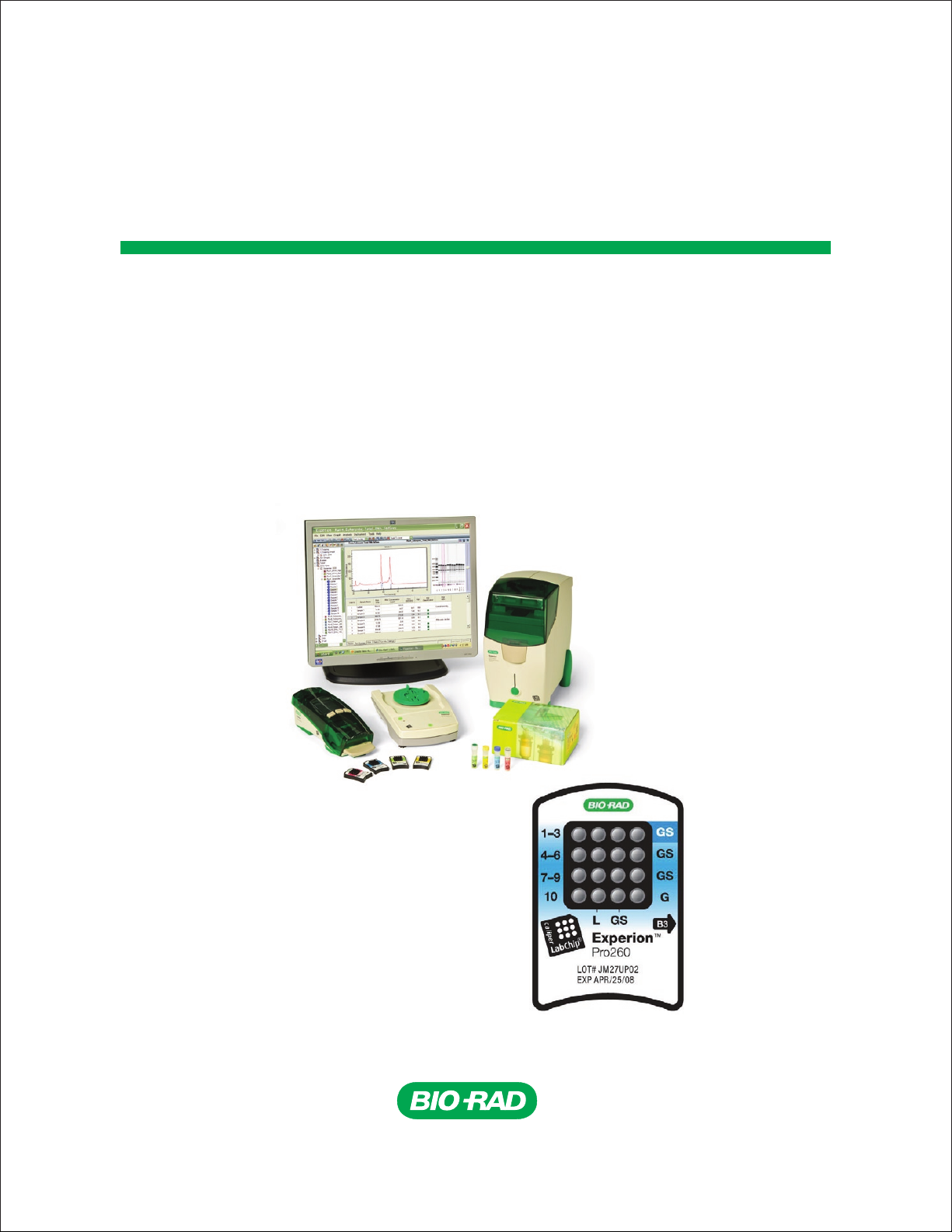
The Experion Pro260 analysis kit is used for protein analysis with the Experion automated electrophoresis system (Figure 1.1). The Experion system employs LabChip microﬂuidic technology to automate protein and nucleic acid electrophoresis by integrating separation, detection, and data analysis within a single platform. The Experion automated electrophoresis system uses smaller sample and reagent quantities than standard analysis methods, and it accomplishes analysis in a single 30-minute, automated step.

The Experion Pro260 analysis kit supplies the microﬂuidic chips, reagents, and instructions required to separate and analyze 10–260 kD proteins under denaturing conditions. The sensitivity of the Experion Pro260 analysis kit is comparable to (though sometimes more sensitive than) colloidal Coomassie Blue staining of SDS-PAGE gels. Each Experion Pro260 chip can analyze up to 10 samples.

For details about how the Experion Pro260 kit analyzes proteins, refer to Appendix A in this manual.

Register your Experion system in order to ensure you receive important updates on software, tech notes, and manuals. Upon installation, a dialog will provide registration instructions.

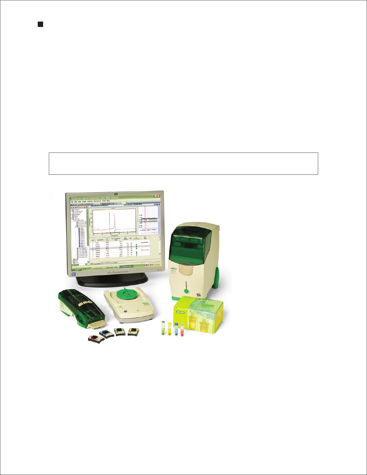
Fig. 1.1. The Experion system. The system includes the following components: 1) automated electrophoresis

station, 2) priming station, 3) vortex station used for nucleic acid analysis only, 4) system operation and data analysis tools (software), and 5) analysis kits, which include the (a) chips and (b) reagents for protein (Pro260 kit), standardsensitivity RNA (StdSens kit), high-sensitivity RNA (HighSens kit), and DNA (DNA 1K and 12K kits) analyses.

2 Technical Support: 1-800-4BIORAD • 1-800-424-6723 • www.bio-rad.com

Experion Pro260 Analysis Kit

1.2 Kit Components

Table 1.1. Components of the Experion Pro260 analysis kit.

Item Description Volume (per Vial) 10-Chip Kit

Pro260 chip Microﬂuidic chips used for protein separation 10 chips

Cleaning chip Chip used for cleaning electrodes 1 chip

Pro260 gel Proprietary polymeric sieving matrix 520 µl 3 vials

Pro260 stain Proprietary ﬂuorescent dye 45 µl 1 vial

Sample buffer Buffer for protein sample preparation; contains a 1.2 kD 400 µl 1 vial lower marker and 260 kD upper marker for alignment of samples to the Pro260 ladder

Pro260 ladder Protein standard containing 9 puriﬁed recombinant proteins 60 µl 1 vial of 10–260 kD and optimized for automated electrophoresis on the Experion system

Spin ﬁlters Used for ﬁltering reagents during sample preparation 3 ﬁlters

1.3 Storage Conditions

Table 1.2. Storage conditions.

Item Storage Shelf Life

Experion Pro260 reagents 4ºC See expiration date on packaging

Experion Pro260 chips Ambient See expiration date on packaging

Gel-stain solution (GS, prepared) 4ºC 1 month from ﬁltration (can be reﬁltered once)

Gel (G, prepared) 4ºC 1 month from ﬁltration (can be reﬁltered once)

1.4 Specifications

Number of sample wells per chip 10

Sample volume required 4 µl

Total run time ~30 min per chip

Protein sizing range 10–260 kD

Limit of detection 2.5 ng/µl carbonic anhydrase (10 ng total) in 1x PBS; similar to colloidal Coomassie Blue G-250 stain

Linear dynamic range 5–2,000 ng/µl (bovine serum albumin in 1x PBS)

Technical Support: 1-800-4BIORAD • 1-800-424-6723 • www.bio-rad.com 3

Experion Automated Electrophoresis System

1.5 Additional Requirements

Experion automated electrophoresis station

Experion priming station

Microcentrifuge (1,000–10,000 x g)

Heating block or water bath set at 95–100°C

Benchtop vortexer

Aluminum foil

Calibrated pipets and narrow-bore tips (for example, VWR #87001-688 or Rainin #L-10F)

Microcentrifuge tubes, 0.5 or 1.5 ml

Deionized water, 0.2 µm-ﬁltered (ReadyPrep™ proteomics grade water, catalog #163-2091)

β-Mercaptoethanol (catalog #161-0710)

Benchtop centrifuge (optional, catalog #166-0612)

Extra spin ﬁlter for additional ﬁltration steps (as needed, catalog #700-7254)

Experion electrode cleaner (catalog #700-7252)

4 Technical Support: 1-800-4BIORAD • 1-800-424-6723 • www.bio-rad.com

Essential Practices

Experion Automated Electrophoresis System

2.1 Storing and Preparing Samples and Reagents

Store all Experion™ Pro260 reagents at 4°C when not in use. Do not store reagents at room temperature for >2 hr, as this will shorten their shelf life.

Before use, allow all kit reagents to equilibrate to room temperature (~15–20 min). Once thawed, gently vortex all kit reagents before use. Before opening the tubes, quickly centrifuge them to collect solution to the bottoms of tubes.

If the Pro260 gel has frozen, discard it.

Protect the stain, sample buffer, and gel-stain solution (GS) from light: store these solutions in a dark place and keep them covered with foil when using them.

The Pro260 stain contains DMSO, which is hygroscopic. Cap tightly.

Use GS and ﬁltered gel (G) for up to 1 month. After that, GS and G can be reﬁltered once again.

Prepare samples in either reducing or nonreducing sample buffer, but always prepare Pro260 ladder in reducing sample buffer.

Do not use coated or treated pipet tips or microcentrifuge tubes (for example, siliconized polypropylene) for preparation of kit reagents or samples. Use of treated tips or tubes may cause separation artifacts.

Use 0.2 μm-ﬁltered or ReadyPrep™ proteomics grade water. Do not use autoclaved water for sample or reagent preparation.

If possible, use sample protein concentrations (before preparation with the Pro260 sample buffer) that are near the middle of the linear dynamic range.

2.2 Priming and Loading the Chip

To avoid contamination, wear gloves and handle chips by the edges. Never touch the glass portions of the chip.

Load the chip on a benchtop or in the priming station. Never load a chip in the electrophoresis station.

Avoid sources of dust and other contaminants when preparing samples and loading the chip. Foreign particles in reagents, samples, or the wells of the chip interfere with separation. Remove chips from their packaging immediately before use.

It may be easier to load the chip on a white background. Tilt the chip to look for bubbles.

Use narrow-bore pipet tips for loading the chip (for example, VWR #87001-688 or Rainin #L-10F).

To avoid introducing air bubbles, do the following (for more help with chip loading, refer to the Experion Training Video in the Experion software Help section under Contents and Index > Contents > Appendices > Technical Videos):

Insert the pipet tip all the way to the bottom of the chip well when dispensing liquids

(this reduces the possibility of trapping air)

Hold the tip vertically, perpendicular to the chip surface. Holding the tip at an angle

may trap air bubbles at the bottom of the well

When expelling liquid, dispense slowly and only to the ﬁrst stop on the pipet. Using the

second stop introduces air and bubbles into the liquid. Reverse pipetting is acceptable

6 Technical Support: 1-800-4BIORAD • 1-800-424-6723 • www.bio-rad.com

Experion Pro260 Analysis Kit

Dislodge bubbles at the bottom of a well with a clean pipet tip, or remove the solution and load it again.

Use a primed and loaded chip within 5 min of loading. When chips are not used within this time, reagents may evaporate, leading to poor results or a chip performance error.

Fill all the chip wells when running an analysis. Use blank samples (prepared with water instead of sample) or replicates if necessary. All 16 electrode pins must be in contact with liquid; otherwise, an IV (current voltage) check failure error will occur.

2.3 Running the Analysis

Place the electrophoresis station on a stable surface, where it will not be subjected to vibrations or other movement, and away from direct sunlight and all other potential sources of extreme heat.

Power on the electrophoresis station before launching Experion software.

The ﬁrst time that the Experion electrophoresis station is used, conﬁrm that communication has been established between the software and electrophoresis station before preparing the reagents.

Do not open the lid of the electrophoresis station during a run. The run will abort if the lid is opened.

2.4 General Maintenance

For recommendations on general instrument maintenance, refer to the Experion system manual (bulletin 10001312).

Clean the electrodes after each run (routine cleaning). Cleaning maintains the instrument in optimum condition and prevents buildup and cross-contamination of reagents and samples.

Perform the deep cleaning procedure described in Appendix B to clean the electrodes:

Prior to ﬁrst use of the Experion electrophoresis station

Whenever contamination is suspected or visible (for example, salt deposits or other

precipitates) on the electrodes

Whenever a chip has been left in the electrophoresis station for an extended period of time

(for example, overnight)

Never store the cleaning chip inside the electrophoresis station. Store the empty cleaning chip covered to keep the wells clean. A new cleaning chip is included with every box of chips.

2.5 Experion Video Tutorials

For additional information, view the video tutorials available online at www.bio-rad.com:

North America: Home > Life Science Research > Support > Tutorials > Electrophoresis and Blotting > Experion System Training

Other: Home > Life Science Research > Electrophoresis > Automated Electrophoresis > Experion Training Videos

Technical Support: 1-800-4BIORAD • 1-800-424-6723 • www.bio-rad.com 7

Experion Automated Electrophoresis System

8 Technical Support: 1-800-4BIORAD • 1-800-424-6723 • www.bio-rad.com

Experion™ Pro260 Assay

Procedure

For an abbreviated version of this protocol, refer to the Quick Guide provided with the kit.

Experion Automated Electrophoresis System

3.1 Set Up the Electrophoresis Station

1. If needed, perform a deep cleaning of the electrodes (see Appendix B for instructions).

2. Power on the computer and then power on the Experion electrophoresis station by pushing the green button in the center of the front panel. The steady green LED above the button indicates that the unit is on.

3. Launch Experion software. If the instrument and computer are communicating properly:

A green dot and the last 4 digits of the instrument serial number appear in the lower right corner

of the software screen

The electrophoresis station icon appears in the upper left corner

When there is no connection, these indicators are absent and a grayed-out instrument icon appears in the upper left corner of the software screen.

3.2 Equilibrate the Kit Reagents

1. Set a heating block or water bath to 95–100°C. You will use this heating block to denature the samples and Pro260 ladder later in the protocol.

2. Equilibrate the following kit reagents to room temperature for ~15–20 min:

Pro260 stain (blue cap)

Pro260 sample buffer (yellow cap)

Pro260 ladder (red cap)

2 tubes Pro260 gel (green cap)

3. Vortex the contents of each tube and brieﬂy centrifuge the solutions to the bottoms of the tubes. Make sure the Pro260 stain solution (blue cap) is thawed before proceeding.

If the gel-stain solution (GS) and ﬁltered gel (G) were prepared previously, equilibrate them to room temperature. Use the GS and G within 1 month of preparation. After 1 month, reﬁlter them before use. Keep both the G and GS at room temperature and covered until ready for use.

3.3 Filter the Gel and Prepare the Gel-Stain Solution

1. Prepare the GS by adding 20 µl Pro260 stain (blue cap) to a tube of Pro260 gel (green cap, 520 µl). Vortex the GS for 10 sec at the highest setting and then spin it down brieﬂy in a microcentrifuge.

2. Transfer the GS to a spin ﬁlter, and transfer the contents of the other Pro260 gel (green cap) into another spin ﬁlter. Label and date the tubes.

3. Centrifuge both spin ﬁlters for 5 min at 10,000 × g. Inspect the tubes to ensure all of the gel passed through the ﬁlters, and then discard the ﬁlters. Cover the GS with foil.

10 Technical Support: 1-800-4BIORAD • 1-800-424-6723 • www.bio-rad.com

Experion Pro260 Analysis Kit

3.4 Prepare the Sample Buffers

Separate protein samples under either reducing or nonreducing conditions, but always use reducing conditions for separation of the Pro260 ladder. Reduced and nonreduced samples can be run on the same chip. Prepare fresh sample buffer daily.

3.4.1 Reducing Conditions

For each chip, combine 1 µl β-mercaptoethanol and 30 µl sample buffer (yellow cap). Vortex and spin down brieﬂy. Protect the sample buffer from light.

At pH <7, reducing agents such as β-mercaptoethanol and DTT are less effective; use 5–7.5 mM tributylphosphine (TBP) or tris(2-carboxyethyl)phosphine (TCEP) instead. Otherwise, neutralize the buffer or use buffers of higher pH before preparing samples for Experion runs.

3.4.2 Nonreducing Conditions

Prepare two stocks of sample buffer: one reducing (for the Pro260 ladder) and one nonreducing (for the protein samples).

1. For each chip, transfer 30 µl sample buffer (yellow cap) to 2 microcentrifuge tubes.

2. Add 1 µl β-mercaptoethanol to one tube (reducing sample buffer) and 1 µl deionized water to the other (nonreducing sample buffer). This generates enough nonreducing sample buffer for 10 samples. Vortex the tubes and cover them with foil to protect them from light.

3.5 Prepare the Samples and the Pro260 Ladder

Each chip can analyze up to 10 protein samples. All wells of a chip must be ﬁlled for the electrophoresis station to operate properly.

The total protein concentration, including any added user-deﬁned internal standards, in all starting samples should be toward the middle of the linear dynamic range of the assay, if possible.

1. Prepare the Pro260 ladder by combining 4 µl Pro260 ladder (red cap) and 2 µl sample buffer with β-mercaptoethanol (reducing sample buffer) in a microcentrifuge tube.

2. Prepare the samples by combining 4 µl sample and 2 µl sample buffer (Section 3.4) in a microcentrifuge tube.

3. Vortex all tubes brieﬂy and spin down in a microcentrifuge for a few sec.

4. Heat the samples and Pro260 ladder at 95–100°C for 3–5 min. Spin down the tubes in a microcentrifuge for a few sec.

5. Add 84 µl deionized water to each tube and vortex brieﬂy to mix. Do not modify this step to adjust sample concentration.

Both the diluted samples and the Pro260 ladder are stable for several hours when stored at room temperature and protected from light.

Technical Support: 1-800-4BIORAD • 1-800-424-6723 • www.bio-rad.com 11

Experion Automated Electrophoresis System

3.6 Prime the Chip

Start the run within 5 min of priming and loading the chip. For help with chip loading, refer to the Experion Training Video: Chip Loading, available in the Experion software Help section under Contents and Index > Contents > Appendices > Technical Videos.

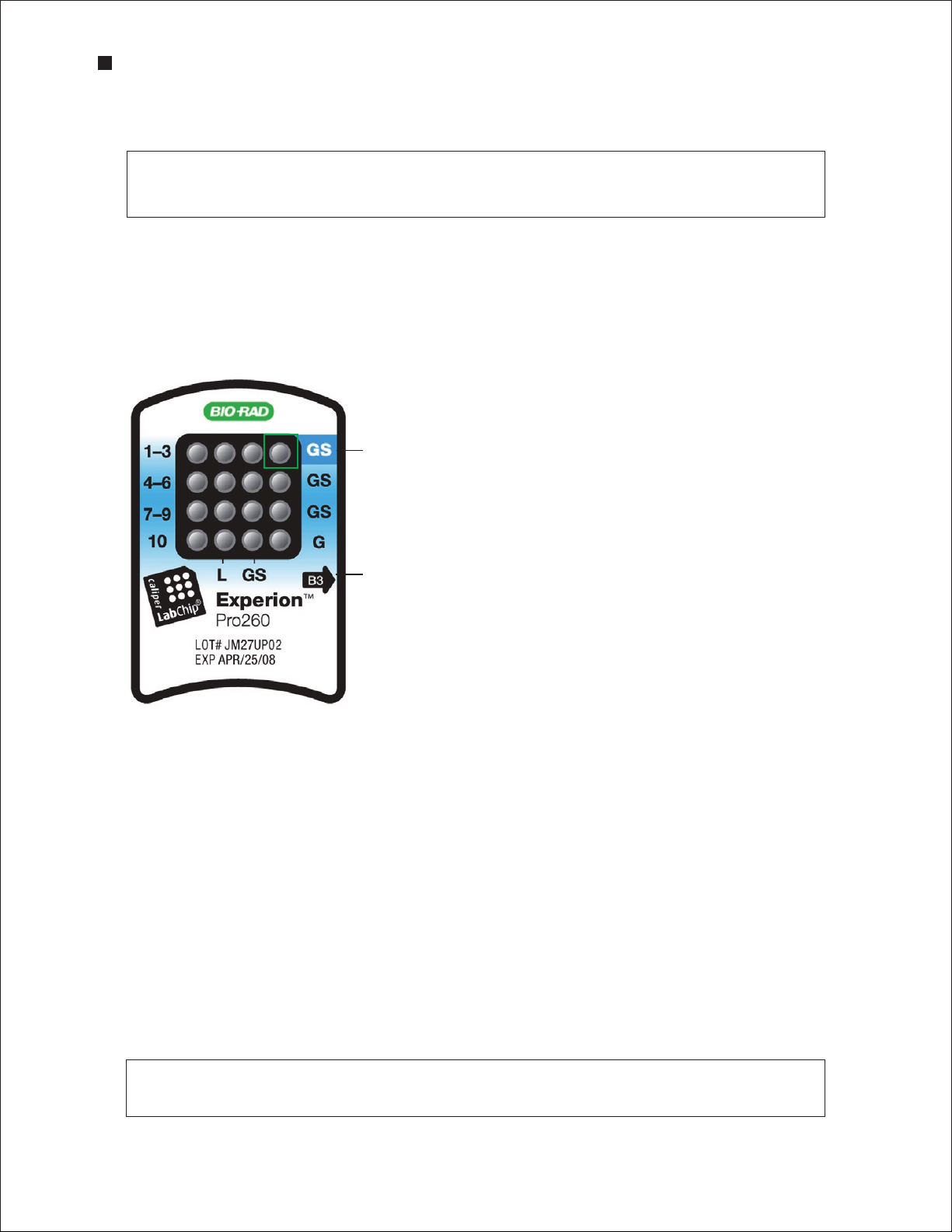
1. Pipet 12 µl GS into the top right well of the chip (highlighted and labeled GS, gel priming well) (Figure 3.1). Insert the pipet tip vertically and to the bottom of the well when dispensing. Dispense slowly to the ﬁrst stop on the pipet, and do not expel air at the end of the pipetting step.

2. On the priming station, set the pressure setting to B and the time setting to 3, as speciﬁed by the alphanumeric code on the chip (Figure 3.1).

Gel priming well

Priming code

Fig. 3.1. Experion Pro260 chip. The locations of the gel priming well (GS, highlighted) and alphanumeric priming code are indicated.

3. Open the Experion priming station and place the chip on the chip platform, matching the arrow on the chip with the alignment arrow on the chip platform. A post on the chip prevents insertion in the wrong position. Do not force the chip into position.

4. Close the priming station by pressing down on the lid. The lid should snap closed.

5. Press Start. A “Priming” message appears on the screen of the priming station, and the timer counts down. Priming requires approximately 60 sec. Do not open the priming station during countdown.

6. An audible signal and “Ready” message indicate that priming is complete. Open the priming station and remove the chip. If the lid sticks, press down on it while pressing down on the release lever.

7. Turn the chip over and inspect the microchannels for bubbles or evidence of incomplete priming. If the chip is primed properly, the microchannels will be difﬁcult to see (it may be helpful to compare a primed chip to a new, unused chip). If you detect a problem, such as a bubble or incomplete priming, prime a new chip.

8. Place the chip on a clean surface for loading.

Bubbles forced into microchannels during priming take the shape of the microchannel and are elongated, not round.

12 Technical Support: 1-800-4BIORAD • 1-800-424-6723 • www.bio-rad.com

Experion Pro260 Analysis Kit

3.7 Load the Chip

1. Using a pipet, remove and discard any remaining GS from the gel priming well. Pipet 12 µl GS into all 4 wells labeled GS (including the gel priming well, Figure 3.2).

2. Pipet 12 µl ﬁltered gel (G) into the well labeled G (Figure 3.2).

3. Pipet 6 µl of each diluted sample into sample wells 1–10.

4. Pipet 6 µl diluted Pro260 ladder into the ladder well labeled L (Figure 3.2). Use the Pro260 ladder within 8 hr of preparation. Every chip must have Pro260 ladder loaded into the ladder well labeled L.

Load 6 µl sample into wells 1–10

Load 6 µl ladder into well labeled L

Fig. 3.2. Experion Pro26 0 chip. Wells for loading GS, G, samples, and ladder are indicated.

Load 12 µl GS into all 4 wells labeled GS

Load 12 µl G into well labeled G

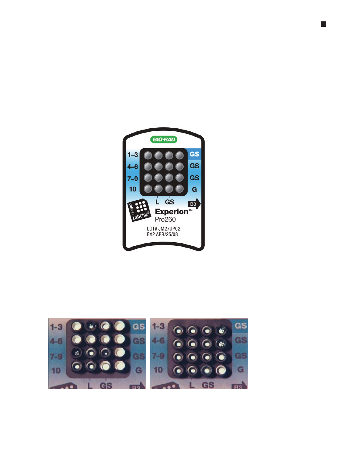
5. Inspect all wells for bubbles by holding the chip above a light-colored background and looking through the wells (Figure 3.3). Dislodge any bubbles at the bottom of a well with a clean pipet tip or by removing and reloading the solution.

6. Place the loaded chip into the Experion electrophoresis station and start the run within 5 min.

Fig. 3.3. Bubble formation during loading of Experion Pro260 chips. Surface bubbles do not generally cause problems during a run, but bubbles at the bot toms of wells must be removed. Lef t, bubbles trapped at the bottom of wells. The GS and G wells and sample wells 1, 3, and 4– 6 contain no solution. Wells 8, 10, and L are ﬁlled properly and have no bubbles, but large bubbles have formed at the bot toms of wells 7 and 9 (note the difference in the diameter of the light-colored circles in wells 8 and 9). Right, bubbles have formed at the surface of the three GS wells on the right side of the chip; the rest of the wells have no bubbles.

Technical Support: 1-800-4BIORAD • 1-800-424-6723 • www.bio-rad.com 13

Experion Automated Electrophoresis System

3.8 Run the Pro260 Analysis

1. Open the lid of the electrophoresis station by pulling the release latch. Place the primed and loaded chip on the chip platform and close the lid.

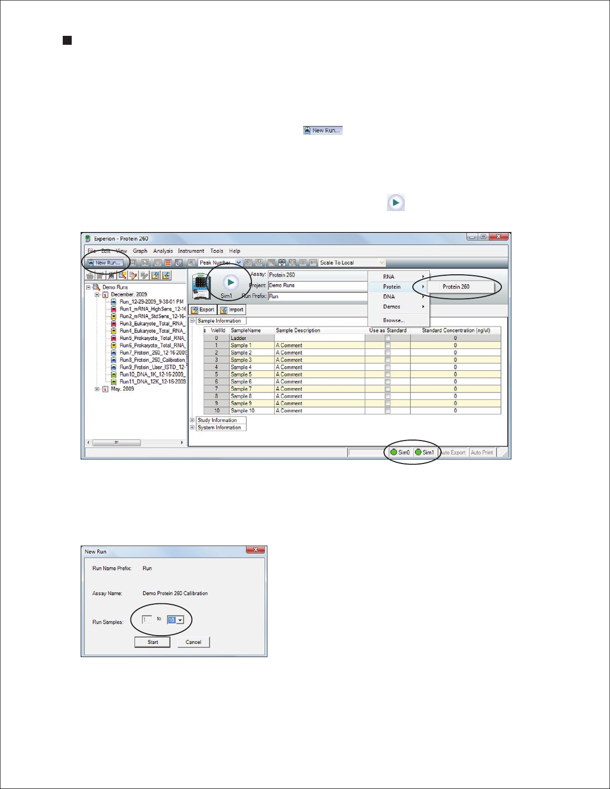
2. In the Experion software toolbar, click New Run . In the New Run screen (Figure 3.4), from the Assay pull-down list, select Protein > Protein 260.

3. Either select a project folder for the run from the Project pull-down list or create a new project folder by entering a name in the Project ﬁeld or by selecting File > Project > New. The project folder appears in the project tree.

4. Enter a name for the run in the Run Preﬁx ﬁeld and click Start Run .

Fig. 3.4. Details of the N ew Run screen. The green dot in the lower right corner indicates that communication between the ele ctrophoresis station and Experion software has been established.

5. In the New Run dialog (Figure 3.5), select the number of samples to be analyzed. Though all wells are ﬁlled, the Experion system stops the analysis when it reaches the number of samples entered.

Fig. 3.5. New Run dialog. The Experion system stops analysis when it reaches the number of samples entered.

14 Technical Support: 1-800-4BIORAD • 1-800-424-6723 • www.bio-rad.com

Experion Pro260 Analysis Kit

6. Click Start. The green LED in the center of the front panel on the electrophoresis station blinks, and the system performs a number of checks: it conﬁrms that a chip has been inserted, that all wells contain liquid, that electrical connections are made, etc. A calibration counter marks the progress of these calibrations at the upper right of the screen.

Do not open the lid of the Experion electrophoresis station until the run is complete. The lid does

not lock. Opening the lid aborts the run.

An “IV Check Error” message indicates the system cannot make electrical contact in one of the wells. This often means there is a bubble at the bottom of the well. Abort the run, and check the chip for bubbles or empty wells. Reﬁll the affected well(s), and start the run again.

7. During separation, the sample name is highlighted in the project tree and the electropherogram trace, and virtual gel bands appear in real time:

The electropherogram of the sample being separated appears in the electropherogram

view

The lane corresponding to that sample is outlined in pink and has a dark background

To display the electropherogram of another sample, click on either the sample name in the project

tree or on a lane in the virtual gel.

8. When analysis is complete (after ~30 min), the instrument beeps and a window opens indicating the end of the run. Select OK and remove the chip from the chip platform.

9. Clean the electrodes using deionized water within 30 min of each Pro260 chip run.

3.9 Clean the Electrodes

1. Fill a cleaning chip with 800 µl deionized water (0.2 µm-ﬁltered). Gently tap the side of the cleaning chip to remove any trapped bubbles from the wells.

2. Place the cleaning chip on the chip platform in the electrophoresis station, close the lid, and leave it closed for 1 min.

Never store the cleaning chip inside the electrophoresis station. Store the empty cleaning chip covered to keep the wells clean. A cleaning chip is included with each box of chips.

3. Open the lid, remove the cleaning chip, and allow the electrodes to dry for 1 min. Close the lid.

4. Replace the water in the cleaning chip after use to avoid contamination. For storage, remove the water from the cleaning chip and store the chip in a clean location.

Technical Support: 1-800-4BIORAD • 1-800-424-6723 • www.bio-rad.com 15

Experion Automated Electrophoresis System

3.10 Evaluate the Run

When a run is complete, evaluate the run and the analysis of the data by Experion software.

1. Ensure all lanes (ladder and samples) are visible in the virtual gel. The markers (indicated by pink triangles) should be visible in and aligned across all lanes. If the marker peaks are not properly assigned, you may need to include or exclude peaks, or manually set the marker (see Section 6.3).

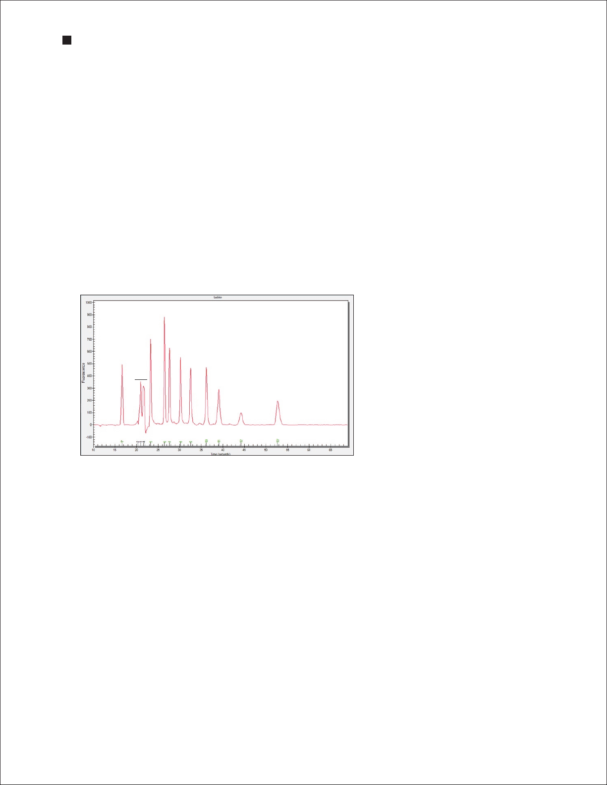
2. Evaluate the separation of the Pro260 ladder. To display the ladder electropherogram, click the ladder well in the project tree, or click on the lane labeled L in the virtual gel. The electropherogram should resemble the one shown in Figure 3.6 and should have the following features (if your ladder does not have these features, see Chapter 7, Troubleshooting for more information):

Two marker peaks and a set of system peaks

Eight Pro260 ladder peaks between the system peaks and upper marker

Flat baseline

Marker peaks at least 20 ﬂuorescence units above the baseline

Pro260 lad der pe aks

Lower marker

System p eaks

Upper m arker

Baseline

Fig. 3.6. Separation of the Pro260 ladder. Note the ﬂat baseline and well-resolved peaks. All identiﬁed peaks are numbered, and the lower and upper markers are indicated by green asterisks (*). The 260 kD protein in the Pro260 ladder is labeled as the upper marker in the Results table.

3. Examine the separation of at least one sample. Click on the sample name in the project tree or on the lane in the virtual gel to view the electropherogram, which should have the following features:

Two well-resolved marker peaks and a set of system peaks

Sample peaks located between the system peaks and upper marker

Flat baseline

If the upper and lower marker peaks are not properly assigned, you may need to include or exclude peaks, or manually set the marker (see Section 6.3).

4. Evaluate the data analysis performed by Experion software (see Chapter 4, Data Analysis). If necessary, change the analysis settings and parameters — including protein quantitation methods — by following the instructions in Chapters 5 and 6.

16 Technical Support: 1-800-4BIORAD • 1-800-424-6723 • www.bio-rad.com

This chapter outlines the basic steps and software features used to view and analyze data. For a more detailed description of Experion™ software and its various functions, refer to the software Help menu. For information on how to customize analysis parameters, refer to Chapter 6, Changing Analysis Settings and Parameters.

Data Analysis

Experion Automated Electrophoresis System

4.1 Viewing Data

The main window of the Experion software user interface contains menus and toolbars, a tree view, and three data views: the electropherogram view, gel view, and results and settings tabs. (Figure 4.1).

Menu ba r

Main sc reen too lbar

Electr opher ogram v iew

Displ ay toolba r

Tree view

Fig. 4.1. Main window of Experion software. The toolbars, menus, and data views are indicated.

Gel vie w

Resul ts and set tings tabs

4.1.1 Managing Run Files and Project Folders in the Tree View

The tree view (Figure 4.2) displays the project tree, a hierarchical tree of all projects and the data ﬁles they contain. Use the project tree and the toolbar above it to:

Open run ﬁles and select samples for viewing

Create project folders

Export and import one or more run ﬁles

Edit names of run ﬁles and project folders

Move runs into project folders

Delete run ﬁles and project folders

Toolbar

Projec t folde r

Run ﬁle

Sample

Fig. 4.2. Tree view details. The project folder name, sample well label, and run ﬁle preﬁx can be customized.

18 Technical Support: 1-800-4BIORAD • 1-800-424-6723 • www.bio-rad.com

Experion Pro260 Analysis Kit

To open a run ﬁle, double-click on it. The run ﬁle opens, displaying the electropherogram and Results tab for the Pro260 ladder, and the virtual gel for the entire run.

To view the data from a sample, click on the sample name or select the corresponding lane in the gel view.

To edit a run ﬁle or project folder name, right-click on it and select Rename Project or Rename Run. Type in the new name.

To import, export, move, or delete ﬁles and folders, click the ocons in the toolbar or use the context menu accessed by right-clicking on the items in the tree view. For more details, refer to the Experion software Help ﬁle.

4.1.2 General Display Controls

Data in the electropherogram view, gel view, and results and settings tabs are linked. Selecting a sample or peak in one area automatically opens or highlights that sample/peak in the other two areas.

To adjust the relative sizes of the three data views and the tree view, click on and drag the border of the view to its new location.

To hide or show one of the three data views, click on the corresponding icon in the display toolbar (located in the upper-right corner of the display, just above the gel view (Figure 4.1).

To zoom in on (expand the view of) a portion of an electropherogram or virtual gel, click on the corner of the area that you would like to enlarge and mouse over to the opposite corner. Double-click anywhere in the electropherogram view to return to the previous view.

4.1.3 Electropherogram View

Experion software plots ﬂuorescence intensity versus migration time to generate an electropherogram for each sample. In the electropherogram, peaks identiﬁed by Experion software are numbered (Figure

4.3). Peaks generated by the markers and used for normalization (for example, the lower and upper

markers) are numbered in green and labeled with an asterisk.

To view the calculated size of a peak or other area of an electropherogram, place the cursor over the peak/area (Figure 4.3). To display the sizes of all the peaks in the electropherogram, select Molecular

Weight in the Select Peak Information pull-down list (main screen toolbar).

Fig. 4.3 . Example of an electropherogr am. All identiﬁed peaks are numbered, and the lower and upper markers are

indicated by a green asterisk (*). Place the cursor over a peak to reveal its size.

Technical Support: 1-800-4BIORAD • 1-800-424-6723 • www.bio-rad.com 19

Experion Automated Electrophoresis System

Double- or right-click on a peak to select it. An inverted black arrow appears above the peak in the electropherogram, and a pink arrow appears above the corresponding band in the virtual gel. The peak number and corresponding data also appear highlighted in the Results table.

Display electropherograms in three different ways:

One at a time (single-well view)

All at once in separate windows (all-wells view)

As superimposed images (overlays)

Single-Well View

This is the default view, which shows the electropherogram data from a single well (Figure 4.4). To return to this display:

1. Click on the sample in the project tree or on the corresponding lane in the virtual gel.

2. In the main screen toolbar, click View Single Well or select View > Single Well.

3. The electropherogram appears. The corresponding lane in the virtual gel is outlined in pink.

Fig. 4.4. Single-well view. As indicated by the arrows, a single electropherogram appears, the name of the sample is highlighted in the project tree, and the corresponding lane in the vir tual gel is outlined.

All-Wells View

To display all electropherograms simultaneously (Figure 4.5):

1. In the main screen toolbar, click View All Wells or select View > All Wells.

2. Electropherograms for each sample populate the electropherogram view (Figure 4.5). Use the

scroll bar to scroll through the electropherograms, or minimize the results and settings table to accommodate the multiple electropherograms.

3. To select and expand a particular electropherogram, double-click on it. The data appear in a

single-well view.

20 Technical Support: 1-800-4BIORAD • 1-800-424-6723 • www.bio-rad.com

Experion Pro260 Analysis Kit

Scroll b ar

Fig. 4.5. All-wells view.

All electropherograms are shown in the electropherogram view. Use the scroll bar to view electropherograms.

Electropherogram Overlays

Superimpose (overlay) multiple electropherograms to facilitate direct comparison among proﬁles. To overlay a subset of electropherograms (Figure 4.6), use one of the following options:

Move into the single-well view and, in the main screen toolbar, click Start Overlay .

Select wells (lanes) in the virtual gel. Each gel lane that is displayed in the electropherogram is outlined. To end the overlay, click End Overlay

Select the lanes in the virtual gel while holding the Ctrl key (for noncontiguous, individual

lanes) or the Shift key (for lanes next to the original lane selected). To exit, click on a lane in the virtual gel or on a sample name in the project tree

Select Analysis > Start Overlay. Select the lanes to overlay. To end the overlay, select

Analysis > End Overlay

Electropherograms appear superimposed in a single window, each in a different color. (The colors cannot be changed.) The sample name appears at the top of the electropherogram, in a color that corresponds to the trace. The ﬂuorescence scale of the overlay electropherogram is based on the sample that is selected ﬁrst; therefore, select the sample with the highest peaks ﬁrst.

Fig. 4.6. Electropherogr am overlay. Electropherograms are

shown in different colors, and the corresponding lanes in the virtual gel are outlined. In this example, lanes 2, 5, and 7 are superimposed using the overlay feature.

Technical Support: 1-800-4BIORAD • 1-800-424-6723 • www.bio-rad.com 21

Experion Automated Electrophoresis System

Peak Labels

Experion software automatically labels detected peaks with numbers for easy identiﬁcation, and the upper and lower markers used for normalization are indicated in green and with an asterisk (*).

To change the type of label displayed, select Graph > Peak Info (or use the pull-down list in the main screen toolbar) and select one of the following options:

No Peak Info — displays no peak information

Peak Number — uses sequential numbers for peak identiﬁcation (default selection)

Peak Time — uses peak migration time (min:sec) for peak labels

Peak Height — uses peak height in units of ﬂuorescence intensity for peak labels

Peak Cor. Area — uses calculated (corrected) peak area for peak labels

Molecular Weight — uses calculated mass (molecular weight, kD) for peak labels

Peak Concentration — uses calculated relative concentration (ng/μl) for peak labels

Electropherogram Tags (Annotations)

To annotate a peak in the electropherogram, right-click on the peak and select Add Tag (Figure 4.7). A tag is automatically generated with the peak information selected (for example, peak number).

To edit a tag, right-click on it, select Edit Tag, and change the information. Click OK.

To annotate a region in the electropherogram, right-click in the region and select Add Tag. In the Edit Tag dialog, enter the annotation and click OK.

To move a tag, click and drag the label to the desired place in the electropherogram.

Fig. 4.7. Example of tagged (annotated) peaks in an electropherogram.

22 Technical Support: 1-800-4BIORAD • 1-800-424-6723 • www.bio-rad.com

Experion Pro260 Analysis Kit

4.1.4 Gel View

Experion software converts electropherogram data into densitometric bands, which appear in the virtual gel (Figure 4.8). Each lane of the virtual gel corresponds to a different sample, and all samples from a chip are shown in a single gel view. When a sample is selected for view as an electropherogram, the corresponding lane in the virtual gel is outlined in pink.

Place the cursor over an area in the virtual gel to view its estimated size in kilodaltons (“kDa”). If a band corresponds to a peak identiﬁed by Experion software, view the peak number and calculated size, concentration, and percentage of total protein by placing the cursor over the band (Figure 4.8).

Right-click on a band to select it. A pink arrow appears above the selected band in the virtual gel, and an inverted black arrow appears above the corresponding peak in the electropherogram. The peak number and corresponding data also appear highlighted in the Results table. Only one peak can be selected at a time.

To select a different color scheme, choose View > Gel Color and select a color from the list. By default, the gel view displays bands as black signals on a white background.

To change the contrast of the bands, use the sliding cursor (Figure 4.8). Changing the contrast does not change the data, but it may improve visualization of faint bands in the virtual gel.

Sliding cursor

Fig. 4.8 . Gel view. Place the cursor over a band in the gel view to display the peak number, size, concentration, and % of total protein. Move the sliding cursor to adjust band intensity.

4.1.5 Results and Settings

The six results and settings tabs (Figure 4.9) present options for viewing, customizing, and analyzing the separation data (see Section 4.3, Using Results and Settings to View and Annotate Data).

Fig. 4.9. Results and settings. Shown is the Results table for a single sample.

Technical Support: 1-800-4BIORAD • 1-800-424-6723 • www.bio-rad.com 23

Experion Automated Electrophoresis System

4.2 Changing the Fluorescence Intensity Scale

To display more or less detail in the electropherogram traces and lanes in the virtual gel, use the options available under the Graph menu, which determine the scale used for the y-axis (ﬂuorescence intensity) of electropherograms and deﬁne the relative scale intensity of the lanes in the virtual gel (Figure 4.10):

Scale To Selected — uses the ﬂuorescence value of the tallest peak in a selected

electropherogram to set the scale of the y-axis for all the other samples. Use this option when comparing (overlaying) a sample with a high-intensity peak and one with a less intense peak

Scale To Global — uses the ﬂuorescence value of the tallest peak from all samples to set

the scale of the y-axis for all the samples. Use this option to adjust the virtual gel to be most similar to an SDS-PAGE separation

Scale To Local (default) — uses the ﬂuorescence value of the tallest peak in each

electropherogram to set the scale of the y-axis for that electropherogram: each sample is scaled separately. This is the best way to view protein electropherograms and sample details

Scale To Selected Peak — uses the ﬂuorescence value of the selected peak to set the

scale of the y-axis for all samples

Scale To Sel ected

Fig. 4.10. Options for modifying the ﬂuorescence intensity scale. Examples of how each option affects the display of a vir tual gel are shown.

Scale To Glo bal

Scale To Loca l

Scale To Sel ected Pe ak (Lane 11)

24 Technical Support: 1-800-4BIORAD • 1-800-424-6723 • www.bio-rad.com

Experion Pro260 Analysis Kit

4.3 Using Results and Settings to View and Annotate Data

The following options appear under the results and settings tabs:

Results — summarizes analysis data for all detected peaks. The data in this table can be

exported (see Section 4.5.2, Exporting Data Files to Other Applications). To view the results of a particular sample, click the electropherogram in the all-wells view or lane in the gel view, or select that sample from the project tree. Alternatively, use the arrows in the main screen toolbar to navigate through the samples. See below for instructions on how to customize the types of data shown under this tab

Run Summary — displays a run summary for all wells; right-click to export the data

Protein Search Result — summarizes user-deﬁned known proteins: lists the samples

that contain a peak that ﬁts with the search of size, or molecular mass as deﬁned under the Protein Search Criteria tab and performs statistical calculations for the size, concentration, and percentage of total protein for each peak identiﬁed

Protein Search Criteria — used to compare statistics for speciﬁc proteins in the samples

(see Section 6.1, Designating and Searching for Speciﬁc Proteins for information on how to designate and then search for known proteins)

Run Info — used to enter sample names and comments after a run is ﬁnished (see below

for instructions)

Settings — used mostly for troubleshooting, but can be used to edit the parameters used

to identify peaks (see Section 6.5, Changing Peak Finding Parameters, or the Experion software Help ﬁle for more details about these settings)

To customize the types of data shown under the Results tab:

1. Right-click on any of the column headers in the Results tab (or click the arrow to the left of the column header). The Column Selector dialog opens.

2. Use the arrow keys to show, hide, or change the order of display of any of the available headers. For detailed explanations of each setting, refer to the software Help ﬁle.

3. Click OK to save the changes, or click Cancel to close the dialog without saving the changes.

Under the Results tab, total concentration data appear at the bottom of the table. This calculation represents the total protein concentration of the original sample. See Bio-Rad bulletins 5299, 5784, and 5423 to learn more about comparing these calculations to data gathered by other methods.

To enter sample names and descriptions:

1. Click the Run Info tab and then click on the plus sign (+) next to Sample Information.

2. Click on any active cell, enter the sample names and descriptions, and click Apply. Click File/Save to save the changes. The sample name appears above its electropherogram.

To enter other information about the experiment:

1. In the Run Info tab, click the plus sign (+) next to the Study Information and/or System Information area(s).

2. Double-click in any blank ﬁeld, enter the information, and click Apply. Click File/Save.

Technical Support: 1-800-4BIORAD • 1-800-424-6723 • www.bio-rad.com 25

Experion Automated Electrophoresis System

4.4 Comparing Data from Different Runs

Experion software allows you to overlay runs from different chips (same assay type), enabling direct comparison of electropherograms and virtual gels from multiple chips. You can save and edit this new virtual chip, but you will not be able to make any new calculations. All calculations in the Results table carry over from the original runs.

In security mode, all run comparisons are saved and cannot be deleted.

1. Click Create a New Compare Run or select Analysis > New Compare Run. In the Compare Runs Setting dialog, enter a name for the comparison in the Compare Name ﬁeld.

2. Select the project in which you wish to store the comparison from the Target Project pull-down list.

3. Select the assay from the Assay Type pull-down list and click Next. The Compare Runs dialog opens, displaying only runs of the same assay type.

4. Double-click to expand the run ﬁles you want to compare, or select a run ﬁle and click List Samples.

5. Click the run ﬁle or sample(s) and use the arrows to move them to and from the Compare ﬁeld. To select several lanes at a time, click the sample names while holding the Ctrl or Shift key. To open a window displaying the selected samples in a gel view, click Show Gel Lanes.

Experion software accepts up to 40 samples for comparison (the default is 30). To change the number of wells used, select Tools > Options. Under the Advanced tab, change the number under Visible Compare Runs Gel lanes.

Only one ladder can be used per comparison. If a ladder is not selected, the ladder used in the ﬁrst run ﬁle is used as the ladder for the entire virtual chip. If an additional ladder is inserted in the virtual chip, it is treated as a sample.

6. Select Realign Data to align the results of all the runs and click OK. The separations appear together in one window as a single experiment. In the Results table, the sizes and concentrations for proteins in each sample are unchanged; the original sizes and concentrations are shown.

7. To change the lanes used in the run comparison:

a. Open a run comparison by double-clicking the ﬁle name in the tree view and then clicking Edit

Compare Run or selecting Analysis > Edit Compare Run.

b. Select the samples you want to add or delete, and use the arrows to add or remove them from

the comparison.

c. To view the samples within a run, double-click the run ﬁle or select it and click List Samples.

8. Click OK to process the changes and view the results.

26 Tech Support: 1-800-4BIORAD • 1-800-424-6723 • www.bio-rad.com

Experion Pro260 Analysis Kit

4.5 Saving, Exporting, and Printing Data

4.5.1 Saving Data Files

Data are automatically saved to a run ﬁle. Names for run ﬁles are given according to the selection made in the Run Files tab of the Options dialog.

To designate a new name for a ﬁle, select File > Save As and enter the desired name.

To view the selections or make changes in the automatic naming of ﬁles, select Tools > Options > Run Files. The following options appear:

Create Run name by combining — select the options to be added to the ﬁle name.

Options include the preﬁx (enter the desired characters), assay class (adds the assay type to the ﬁle name), instrument name, date, and time

Run ﬁle folder — choose between default (saves ﬁles to the directory C:\Program Files\

BioRad Laboratories\Experion Software\Data) and custom (enables navigation and selection of another folder)

Create daily folders — select to enable creation of daily subfolders by date. When this

option is selected, the software stores all run ﬁles from the same date in a single folder

4.5.2 Exporting Data Files to Other Applications

To export data to another program (for example, Excel software), select File > Export Data. In the Export dialog, select the desired options. For a complete description of all export options, refer to the

Experion software Help ﬁle.

To export ﬁles automatically after a run is completed:

1. Select Tools > Options and click the Advanced tab.

2. Select Auto Export and then click Settings.

3. Select the options for Auto Export and click Apply.

To quickly copy and paste electropherograms, virtual gels or lanes in the gels, or data tables into another application, use the options under the Edit pull-down list.

4.5.3 Printing Data Files

You can print both graphic and tabulated data from a run.

To choose the print options, select File > Print and select the desired options in the Print dialog. For a complete description of all printing options, refer to the Experion software Help ﬁle (search term “printing data”).

To print ﬁles automatically after a run is completed:

1. Select Tools > Options and click the Advanced tab.

2. Select Auto Print and then click Settings.

3. Choose the desired options in the Experion Print dialog and click Apply.

To save or print the data as a PDF ﬁle, select File > Print and select Print PDF.

Technical Support: 1-800-4BIORAD • 1-800-424-6723 • www.bio-rad.com 27

Experion Automated Electrophoresis System

28 Technical Support: 1-800-4BIORAD • 1-800-424-6723 • www.bio-rad.com

Protein Quantitation Methods

Experion Automated Electrophoresis System

5.1 Protein Quantitation Methods

Experion™ software enables protein quantitation by several approaches. The selection of approaches depends on the type of experiment and desired level of accuracy (Table 5.1). Refer to Appendix A and bulletin 5784 for details about the different quantitation methods.

Table 5.1. Protein quantitation methods used by Experion software. Absolute quantitation methods provide greater accuracy than relative quantitation methods. The accuracy of percentage determination is protein dependent.

Calibration Method and Internal Standard Used Single-Point Calibration Curve Quantitation Method Output Upper Marker User-Deﬁned Upper Marker User-Deﬁned

Percentage Determination % Total No internal standard required Concentration Determination

Relative quantitation ng/µl l — — — — l — — Absolute quantitation ng/µl — — l —

— — —

5.2 Performing Percentage Determination

Experion software automatically calculates a percentage of total protein (% total) value for each detected peak and lists the results in the % Total column of the Results table (Figure 5.1). Click on the peak of interest in the electropherogram to highlight the data for that peak.

Fig. 5.1. Results table showing quantitation data for peaks in a sample. Experion software automatically performs % total and relative concentration determinations for each peak identiﬁed in every sample.

To exclude a peak from the % total calculation, right-click on the peak (in either the single-well electropherogram view or Results table) and select Exclude Peak in the context menu. The new calculations for the remaining peaks appear in the Results table.

This change affects a selected sample. To exclude multiple peaks from multiple samples, use the Settings tab and the Peak Find Settings options in the All Wells Settings dialog (see Section

6.4, Excluding a Peak From Analysis and 6.5, Changing Peak Finding Parameters) and adjust the peak detection criteria.

30 Technical Support: 1-800-4BIORAD • 1-800-424-6723 • www.bio-rad.com

Experion Pro260 Analysis Kit

5.3 Performing Relative Quantitation

Experion software also automatically performs quantitation of all peaks in a sample by a single-point calibration to the 260 kD upper marker and presents these data in the Concentration (ng/µl) column of the Results table.

To view these default relative quantitation results, click on the peak of interest in the electropherogram to highlight the data for that peak.

To perform relative quantitation against a different, user-deﬁned internal standard:

Add the standard to the samples at a single concentration, and

Change some of the analysis settings in the software

Selection of the user-deﬁned standard in the software may be done after the run is complete. This enables easy comparison of the relative quantitation results derived by using both the upper marker and the user-deﬁned standard.

To perform relative quantitation with a single concentration of a user-deﬁned internal standard:

1. Prepare the protein samples and reagents as outlined in Section 3.5, except add a known concentration of the internal standard (for example, 500 ng/µl) to each sample. For example, replace half the volume of sample with the internal standard (combine 2 µl sample, 2 µl internal standard, and 2 µl sample buffer).

Do not add the internal standard to the Pro260 ladder.

2. Run the Pro260 analysis.

3. After evaluating the run as described in Section 3.10, select Analysis > Internal Std. and Std Protein Calibration Curve.

4. In the Internal Std. and Std. Protein Calibration Curve window (Figure 5.2), select Use User Internal Standard and enter the name, concentration, and molecular weight (MW) of the internal standard. Click Apply and then Close. The new concentrations appear in the Results table under the Concentration (ng/µl) column (Figure 5.3).

Fig. 5.2. Internal Std. and Std. Protein Calibration Curve window.

Technical Support: 1-800-4BIORAD • 1-800-424-6723 • www.bio-rad.com 31

Experion Automated Electrophoresis System

Fig. 5.3. Results from relative quantitation.

5.4 Performing Absolute Quantitation

Experion software also allows quantitation using a calibration curve generated by a range of known concentrations of that protein (absolute quantitation). In this method:

Different concentrations of the protein are separated in different sample wells

The peak areas of the different concentrations are compared to the peak area of an internal

standard. As with relative quantitation, either the upper marker or a user-deﬁned protein can be used as the internal standard

The protein concentrations in the samples are then determined from this calibration curve

Experion software displays the results for both relative and absolute quantitation, enabling easy comparison of the accuracy achieved by these different approaches.

5.4.1 Absolute Quantitation Using the Upper Marker as Standard

1. Prepare a dilution series of 3–6 different concentrations of the protein used for calibration. The total protein concentration in each sample must be within the linear dynamic range of the assay. Prepare these samples with the other samples for Pro260 analysis as described in Section 3.5.

2. In the Run Info tab under Sample Information, designate the wells that contain the proteins for the calibration curve by selecting them in the Use as Standard column (Figure 5.4). Enter their concentrations in the Standard Concentration column and click Apply.

3. Run the Pro260 analysis.

Fig. 5.4. Run Info tab illustrating the creation of a 5-point calib ration cur ve with wells 1–5 .

32 Technical Support: 1-800-4BIORAD • 1-800-424-6723 • www.bio-rad.com

Experion Pro260 Analysis Kit

4. After evaluating the run as described in Section 3.10, select Analysis > Internal Std. and Std Protein Calibration Curve.

5. In the Internal Std. and Std. Protein Calibration Curve window (Figure 5.5), do the following:

a. Under Standard Information, next to Standard Protein Molecular Weight, enter the MW

corresponding to the region where the software searches for a peak, for both the calibrants and the samples. The software checks for a peak in the sample wells that has the entered value (± 5%). If necessary, modify the concentrations of the calibrants by double-clicking on the concentration value and typing in a new value.

b. Ensure that Use User Internal Standard is not selected.

c. Under Calibration Curve Settings, if the protein used for calibration (calibrant) is different or

has a different mass than the protein being quantitated, select Quantitate All Proteins and click Apply. If you do not do this, the software only reports absolute concentrations for peaks that are the same size as the calibrant.

d. Under Calibration Curve Settings, select the Linear Regression to be used.

e. Click Apply to update the calculation. The calibration curve appears and displays the equation

for the linear regression (Figure 5.5). The table below the graphic displays data for the wells containing the standards. Click Close.

6. In the Results tab, the concentration for each protein identiﬁed by Experion software is derived by relative quantitation against the 260 kD upper marker and automatically appears in the Concentration column; the calibrated concentrations of proteins found in the speciﬁed region appear in the Calib. Conc. column.

Fig. 5.5. Internal Std. and Std Protein Calibration Curve window. In this example, a 100 kD protein is used to build a 5-point calibration curve for quantitating a 100 kD sample protein.

Technical Support: 1-800-4BIORAD • 1-800-424-6723 • www.bio-rad.com 33

Experion Automated Electrophoresis System

5.4.2 Absolute Quantitation Using a User-Deﬁned Internal Standard

This is the most stringent method of quantitation. It combines two of the approaches described above:

A calibration curve is generated using known concentrations of a protein, and

A user-deﬁned protein is used as the internal standard

1. Prepare a dilution series of 3–6 concentrations of the protein that you will use for calibration.

2. Add a known concentration of the internal standard to each sample (except the Pro260 ladder), including those that will be used for calibration. Prepare these samples and other samples as described in Section 3.5.

3. Under the Run Info tab, designate the wells that contain the proteins for the calibration curve and enter their concentrations (Figure 5.5). Click Apply and run the Pro260 analysis.

4. After evaluating the run as described in Section 3.10, select Analysis > Internal Std. and Std Protein Calibration Curve.

5. In the Internal Std. and Std. Protein Calibration Curve window (Figure 5.5), do the following:

a. Under Standard Information, next to Standard Protein Molecular Weight, enter the MW

corresponding to the region where the software searches for a peak, for both the calibrants (standards) and the samples. The software checks for a peak in the sample wells that has the entered value (± 5%). If necessary, modify the standard concentrations by double-clicking on the concentration and entering a new value.

b. Select Use User Internal Standard and enter the name, concentration, and size of the internal

standard. Click Apply.

c. Under Calibration Curve Settings, if the protein used for calibration (calibrant) is different or

d. Under Calibration Curve Settings, select the Linear Regression to be used. Click Apply to

update the calculation.

6. The calibration curve appears, displaying the equation for the linear regression. The table below the graphic displays the data for the protein standard samples. Click Close.

7. In the Results table, the concentration for each protein derived by relative quantitation against the user-deﬁned internal standard appears in the Concentration column, and the calibrated concentration (using the calibration curve in conjunction with the user-deﬁned standard) appears in the Calib. Conc. column.

34 Technical Support: 1-800-4BIORAD • 1-800-424-6723 • www.bio-rad.com

Changing Analysis

Settings and Parameters

Once an Experion™ analysis is complete and you have examined the quality of the run and of the data, you can reanalyze the data by changing some of the settings. Most of the steps outlined in this chapter are used for troubleshooting purposes or are optional; they are not required in most analyses.

Experion Automated Electrophoresis System

6.1 Designating and Searching for Specific Proteins

1. Designate and search for speciﬁc proteins in your samples:

a. In the Protein Search Criteria tab, click Add Protein Name , or in the electropherogram,

right-click on a peak and select Add to Protein Search Criteria. The Protein Search Criteria tab opens and contains the mass and tolerance range for that entry.

b. Click in the ﬁeld under Protein Name and enter the protein name.

c. Click in the ﬁeld under Mol Wt and enter the size of the protein in kD.

d. Click in the ﬁeld under the ±s mass column to enter the new value for the tolerance in kD and

exclude wells that are not relevant to the search.

2. A list of all the peaks that ﬁt the criteria appears in the Protein Search Result tab. Separate tables appear for each protein designated in the search criteria list. To exclude a peak, right-click on the peak name in the table and select Exclude Peak.

3. To delete designated proteins (“protein names”) from a search, click Delete Protein Name in the toolbar of the Protein Search Criteria tab.

6.2 Changing Protein Quantitation Parameters

Experion software uses relative quantitation against the upper marker to calculate the concentrations of all the peaks detected in a sample. The calculated concentrations appear in the Results table, under the Concentration (ng/µl) column.

For more information about protein quantitation, including about how to perform relative quantitation against a user-deﬁned standard or to perform absolute quantitation using a calibration curve, refer to Appendix A and the instructions provided in Chapter 5, Protein Quantitation Methods.

6.3 Manually Setting a Marker

To designate a peak as a marker (and change the alignment of a sample), right-click on the peak in either the electropherogram (single-well view) or the Results table and select Manually Set Lower Marker or Manually Set Upper Marker to deﬁne the peak as the new lower or upper marker. Do this if no or incorrect peaks have been selected as the lower or upper marker.

Pink triangles in the virtual gel indicate markers. The markers should be aligned across all lanes.

6.4 Excluding a Peak from Analysis

To exclude one or more peaks from analysis of a single sample, right-click on the peak in either the electropherogram (single-well view) or Results table and select Exclude Peak from the context menu. This change affects only a selected sample.

To exclude multiple peaks from multiple samples, open the Settings tab and use the Peak Find Settings options in the All Wells Settings dialog (see Section 6.5, Changing Peak Finding Parameters) to adjust the criteria by which peaks are detected.

Excluded peaks are not included in total protein calculations. Therefore, excluding a peak from analysis affects percentage determination (% total calculations) for the other peaks in a sample.

36 Technical Support: 1-800-4BIORAD • 1-800-424-6723 • www.bio-rad.com

Experion Pro260 Analysis Kit

6.5 Changing Peak Finding Parameters

The parameters entered tell the peak-ﬁnd algorithm whether a peak is signiﬁcant.

To edit the parameters used by Experion software for ﬁnding peaks in a selected sample/well:

1. Select the sample by clicking on the lane in the virtual gel (or on the sample name in the tree view).

2. Under the Settings tab, edit the parameters under Peak Find Settings:

Slope Threshold — represents the variation in ﬂuorescence units over time required to

detect a peak (accepted values are 0.2–1,000, with lower values yielding more peaks)

Min. Peak Height — minimum height required for a peak to be integrated (accepted values

are 0.1–1,000). Determine the appropriate value for this parameter by zooming in on a small peak in an electropherogram and reading its ﬂuorescence value on the y-axis

Min. Peak Width — minimum amount of time that must elapse before a peak is

recognized (accepted values are 0.1–10, with lower values yielding more peaks)

3. Click Apply to apply the changes and reanalyze the data. Click Save in the main screen toolbar to save the new conditions or click Reset to Default to recover the default settings.

To modify the peak-ﬁnd settings for all sample wells:

1. Under the Settings tab, click the All Well Settings tab or select Analysis > All Wells Settings.

2. In the All Wells Settings dialog, expand Peak Find Settings and select the type of modiﬁcation you would like to apply (see above for descriptions).

3. Click OK to apply changes and Ye s to overwrite the settings. Click Save in the main screen toolbar to save the new conditions. To reset to default settings, click Reset to Default.

Do not adjust the Peak Find Settings values so that the markers are eliminated from analysis.

6.6 Changing General Settings

These settings appear in the Settings tab, in the All Wells Settings dialog under General Settings (Figure 6.1). They apply to all samples in a run.

Data Frequency — displays the rate of data collection in Hz

Display Start Time — displays the time Experion software begins displaying peaks

Display End Time — displays the time Experion software stops displaying peaks

Upper Marker Concentration — displays the concentration of the upper marker

Use Time Corrected Areas — corrects for peaks of different sizes that pass the detector

at different rates

Calibrate All Valid Peaks — select this option if you are running a calibration curve and

want Experion software to calibrate all peaks (this is the same as selecting Quantitate All Proteins in the Internal Std. Protein Calibration Curve window)

Filter Width — determines the width of the polynomial (in sec) to be applied to the data for

ﬁltering (noise reduction). Set this variable to less than twice the width of peaks. Valid values are 0.3–10

Polynomial Order — deﬁnes the power series applied to ﬁt the raw data. Valid values are

1–10, with lower values yielding smoother curves

Technical Support: 1-800-4BIORAD • 1-800-424-6723 • www.bio-rad.com 37

Experion Automated Electrophoresis System

Fig. 6.1. General Set tings options.

6.7 Baseline Modification

To change the method used by Experion software for adjusting the baseline in a selected electropherogram (single sample):

1. Under the Settings tab, select one of the following two options under Algorithm Inclusion Settings (Figure 6.2):

Baseline Correction — (default) subtracts the baseline from the signal. The baseline

represents a slow, rolling component in the signal. Generally, this method affects the original shape of the curve and subsequent calculations. The more complex the baseline, the greater impact subtraction might have on the signal. However, for well-resolved peaks with a slow rolling component, this method can normalize calculations across the chip. If peaks are poorly resolved, baseline correction can cause considerable artifacts

Zero Baseline — subtracts the average baseline value from the signal. This method

does not affect the shape of the curve; it shifts the baseline down to zero. If the Baseline Correction option results in undesirable artifacts (small peaks do not appear, or too many peaks appear), change this setting to see if it remedies the problem

Deselecting both options makes the original signal(s) appear. Sometimes it is important to see the difference between the signals across the chip if no correction is applied.

2. Click Apply to apply the changes and reanalyze the data, and click Save in the main screen toolbar to save the new conditions or choose Reset to Default to recover the default settings.

To edit the parameters used by Experion software for adjusting the baseline for all samples:

1. Either open the Settings tab or select Analysis > All Wells Settings.

2. In the All Well Settings dialog, expand Algorithm Inclusion Settings and select the type of modiﬁcation you would like to apply (see above for descriptions or Figure 6.2). Click OK.

3. In the Experion Application dialog, click OK and Yes to to overwrite the sample settings. Click

Save in the main screen toolbar to save the new conditions. To reset to default settings, click Reset to Default in the Settings tab under All Well Settings.

38 Technical Support: 1-800-4BIORAD • 1-800-424-6723 • www.bio-rad.com

Experion Pro260 Analysis Kit

Fig. 6.2. Algorithm Inclusion Settings window.

6.8 Turning Analysis Off

To turn analysis off, select Analysis > Turn Analysis Off. Analysis remains off for all runs until it is turned back on.

Turning analysis off displays the raw data from a run; it deactivates alignment, shifting the positions of the upper and lower markers in each sample. In addition, the pink arrows (in the virtual gel) indicating the positions of the markers appear only in the ladder lane. With analysis off, the migration of the markers may not be perfectly aligned and the position of the upper marker may drift (Figure 6.3). Turning analysis off can help reveal if a problem is isolated (one or a few wells have markers out of alignment) or is general (alignment problems across the entire chip).

Analy sis on Analysis of f Analy sis on A nalysis off

Fig. 6.3. Effects of turning analysis of f for two samples.

Technical Support: 1-800-4BIORAD • 1-800-424-6723 • www.bio-rad.com 39

Experion Automated Electrophoresis System

6.9 Manual Peak Integration

This function enables deﬁnition or reﬁnement of peak areas for the ladder and all sample lanes.

1. Select a sample and click or select Analysis > Manual Integration to start manual integration.

2. Adjust the baseline by clicking and dragging the dots at the ends of the peaks (Figure 6.4). If a peak in the electropherogram is not detected by the software, right-click on that peak and select Add Peak. Zoom in on the peak for a better view of the baseline.

3. Save any changes by selecting File > Save Run As (use a new ﬁle name), or revert to the original baseline and integration by clicking .

Manual integration applies to individual sample wells. Moving back to automated integration loses changes made during manual integration unless those changes are saved.

Fig. 6.4. Manua l integration mode indicates the beginning and end of peak baselines with blue dots.

40 Technical Support: 1-800-4BIORAD • 1-800-424-6723 • www.bio-rad.com

Troubleshooting

Experion Automated Electrophoresis System

7.1 Electrophoresis and Priming Stations

Error Probable Cause Recommended Action

IV Check Failure

(Experion™ software)

Check Seal

(Priming station)

One or more wells are not ﬁlled correctly, and the electrodes are not immersed

Air bubbles are interfering with the electrical contact in one or more of the wells

An electrode is loose or disconnected Perform a conductivit y test with the cleaning chip or

Lid is not closed Close the lid

The chip is not primed properly Repeat the analysis using a new chip

The priming seal is worn, torn, or clogged Replace the priming seal (catalog #700-7031)

The chip is not positioned correctly in the priming station

The gel-stain solution (GS) was added to the wrong well for priming

Fill all sample wells of the chip with blank or replicate samples

Ensure pipets are properly calibrated

Stop the run, remove the chip, and use a clean pipet tip to remove the sample and apply a new aliquot

When pipetting, inser t the tip vertically and to the bottom of the well. Dispense the liquid slowly. Do not expel air at the end of the pipetting step. Dispense only to the ﬁrst stop on the pipet. Positive (reverse) pipetting may also be used

conductivit y chip from the Experion validation kit (catalog #700-7051). Add 850 µl water to the chip, place the chip in the electrophoresis station, and close the lid. In Experion software, select Tools > Diagnose Instrument and select Conductivity in the Instrument Diagnostics dialog

If the test passes, focus on the sources of error above. If it fails, contact technical support with the results

Align the arrow on the chip with the arrow on the platform

The priming well is highlighted on the chip. Se e Section 3.6, Prime the Chip

No chip detected Chip not positioned properly, empty wells,

Run aborts before all wells are analyzed

or incor rect reagents

The computer power saver options are causing the runs to abort (this is only a problem with Experion software prior to version 3.0)

Make sure chip is positioned prope rly and correct reage nts used

Upgrade to the newest software version

Conﬁrm that all power saver and/or power options are turned off before star ting the assay. Do not let the computer “sleep” during a run. If the computer goes to sleep, the run will abort

7.2 Experion Pro260 Analysis

Error Probable Cause Recommended Action

Concentrations are not reproducible (CV > 20%)

Peaks were not detected in the Pro260 ladder

Sample preparation procedures are inconsistent

An air bubble is at the bottom of the ladde r well or microchannels due to poor priming or sample loading; air bubbles can interfere with the contact between the electrode and the liquid

Use the same reagents and follow the same procedures for each sample and each r un. Do not modify the protocol outlined in Chapter 3 to compensate for protein concentration or sample variabilit y

Check the chip for air bubbles after priming and sample loading:

After priming: turn the chip over and make sure the

microchannels are ﬁlled with gel-stain solution (GS). If the chip is primed correctly, the wells should be hard to see. Compare the primed chip to an unprimed chip if necessary. Do not touch the glass

After sample loading: tilt the chip and view it from different

angles against a light background

42 Technical Support: 1-800-4BIORAD • 1-800-424-6723 • www.bio-rad.com

Experion Pro260 Analysis Kit

Error Probable Cause Recommended Action

No peaks were detected in some samples

No peaks detected in any samples

There is not enough sample in the wells Ensure that pipets are calibrated and that 6 µl solution has

Samples were not prepared properly Review the sample preparation procedure detailed in

Pro260 stain was photobleached Protect the Pro260 stain, gel-stain solution (GS), sample

Particulates are clogging the microchannels Use only high-quality, 0.2 µm-ﬁltered water (such as

Gel-stain solution (GS) is old or has been photobleached

Chip was not primed with the correct pressure and time settings

Particulates are clogging the microchannels Use only high-quality, 0.2 µm-ﬁltered water (such as

been added to the wells

Chapter 3. The Pro260 ladder must be prepared with reducing sample buf fer even when samples are to be separated under nonreducing conditions

buffer, and prepared and diluted samples from light

Prepare new GS; use a new tube of Pro260 stain if necessary

ReadyPrep™ proteomics grade water, not autoclaved water)

Verify that the gel (G) and GS were properly ﬁltered

If using samples that contain particulates, perform a quick microcentrif uge spin of the prepared sample to pellet particulates before loading

Prepare fresh GS

Check settings on the priming station and repeat the analysis with a new chip

ReadyPrep proteomics grade water, not autoclaved water)

Verify that the gel (G) and gel-stain solution (GS) were properly ﬁltered

If using samples, such as cell lysates, that contain particulates, perform a quick microcentrifuge spin of the prepared sample to pellet particulates before loading

Lower and/or upper marker is missing

Electropherogram peaks are much smaller than expected (peaks are <50% of what is expected)

Samples do not contain sample bu ffer or were not prepared properly (if both are missing)

Late migration If only the upper marker is missing, refer to the

Too much stain in the gel-stain solution (GS); sample cannot destain completely, and the background is high; too much stain can contribute to high background (>1,000 RFU) and low sample and ladder peaks

Not enough sample was added Ensure pipets are calibrated

Too much salt in the sample; salt ions compete with the sample ions during injection

One or more components in the sample is beyond the concentration range listed in the compatibilit y table (Appendix C)

Gel-stain solution (GS) is old or has been photobleached

Review the sample preparation procedure in Chapter 3

trouble shooting tips for late migration (below)

Prepare new GS using a new tube of stain. Ensure stain is thawed completely before preparation

Use pipets that accurately deliver volumes of 10 µl or less

Analy ze a dilution series of the sample in water on another chip. If the peak heights and calculated protein concentrations of the diluted sample increase, the salt is too high in the original sample. Determine the proper dilution to minimize the salt effect

Analy ze a dilution series of the sample in water on another chip. Adjust your sample preparation procedure as necessary

Prepare fresh GS

Technical Support: 1-800-4BIORAD • 1-800-424-6723 • www.bio-rad.com 43

Experion Automated Electrophoresis System

Error Probable Cause Recommended Action

Reagents, speciﬁcally the Pro260 stain, were not brought to room temperature prior to use; if stain is not equilibrated to room temperature, it will be more concentrated when it is added to the gel, which may result in signiﬁc antly lower protein peaks and areas

Repeat the analysis with a new chip, new tube of stain, and properly equilibrated reagents

Peaks are small, broad, or missing in some samples, but present in other samples on the chip

Late migration (peaks broaden and are de layed over the course of the r un)

Gel (G) and gel-stain solution (GS) were mislabeled or used improperly. The Pro260 chip contains speciﬁc wells for G and GS: GS wells carry the sample through the microchannels and supply the dye for analysis, and the G well is used for destaining prior to detection. If G and GS are added to the incorrect wells, peaks can be small, crowded, or missing in ele ctropherograms

Pro260 ladder and samples were not completely denatured

Contaminants are prese nt Che ck chemical compatibility char ts (Appendix C) and

Sample pH is lower than 5 Adjust pH of the sample to 5 or above

Air bubbles are interfering with electrical contact in one or more of the wells

Ensure chip was primed with GS

Ensure G was used in the G well and GS was used in all wells marked GS

Heat samples and Pro260 ladder for 3 –5 min at 95–100°C before loading

prepare samples in a dif ferent extraction buffer or dilute them in water, if necessary

Do not use autoclaved water for diluting protein samples or ladder. Use only high-quality, 0.2 µm-ﬁltered water (such as ReadyPrep proteomics grade water)

Turn analysis off (see Section 6.8, Turning Analysis Off, for more information). Late migration is indicated if there is a drift in the migration of the lower marker across the chip and the upper marker migrates later and runs off the top of the gel view. Refer to the troubleshooting tips that follow

Stop the run, remove the chip, and use a clean pipet tip to remove or dislodge the bubbles, or re move and replace the solution in affected wells

When pipetting, inser t the tip vertically and to the bottom of the well. Dispense liquids slowly. Do not expel air at the end of the pipetting step. Dispense only to the ﬁrst stop

Peaks migrating faster than usual; electropherogram appears compressed

Molecular mass (sizing) is incorrect

Electrophoresis station temperature is inappropriate or ﬂuctuating during the run (should be 30– 35°C); there is no cooling unit in the electrophore sis station, so if the temperature changes during the course of a run, the samples will exhibit different separation characteristics

Pro260 ladder peaks and upper and lower markers were improperly assigned by the software

Ensure that the temperature of the room is appropriate and stable, and place the electrophoresis station away from all heat sources, such as windows or ovens

Exclude peaks (follow the instructions in Section 6.4, Excluding a Peak From Analysis) or ma nually assign markers (follow the instructions in Section 6.3, Manually Setting a Marker), if necessary

Sizing should be within 10% of the size seen by SDS-PAGE, except for proteins with high levels of posttranslational modiﬁcation, or highly acidic or basic proteins

44 Technical Support: 1-800-4BIORAD • 1-800-424-6723 • www.bio-rad.com

Experion Pro260 Analysis Kit

Error Probable Cause Recommended Action

Protein quantitation is incorrect

Upper and lower markers were not properly assigned by the software

Pipetting and/or dilution errors occurred during sample preparation or chip loading

Samples are old or have not been stored properly, and the proteins degraded

Samples were not denatured prope rly; regardless of whether re ducing or nonreducing conditions are used, the Pro260 ladder and samples must be heat-denatured for the assay to run properly

Samples do not have the same staining proper ties as the upper marker

Check that both markers were properly assigned. Manually select the marker(s), if necessar y (follow the instr uctions in Section 6.3, Manually Set ting a Marker)

Ensure your calculations and dilutions are corre ct

Ensure that pipets a re calibrated, and use pipets that accurately deliver volumes of 10 µl or less

Do not modify the sample preparation and loading protocols described in this manual

Ensure that the total protein concentration of your samples (including any user-deﬁned internal standards that may be added) is within the linear dynamic range before procee ding with the sample preparation instructions described in Section 3.4; if total protein concentration is unknown, run a Pro260 analysis of a dilution series of your sample

Review the essential practices described in Chapter 2 before initiating another analysis with a new chip

Prepare fresh samples and try the analysis again

Heat the samples and the Pro260 ladder for 3–5 min at 95–100°C before loading them into the chip. Keep the caps of the s ample and ladder tubes closed during heating to prevent loss of vapor and subsequent changes in concentration. Brieﬂy centrifuge the samples before opening

Use a dif ferent internal standard or a calibration curve (see Chapter 5, Protein Quantitation Methods, for more information)

Ghost peaks or contaminants appear in electropherograms

Upper or lower marker is incorrectly identiﬁed

Portion of the electropherogram is incorrectly identiﬁed as a peak

Virtual gel does not resemble an SDS-PAGE separation of the same samples

Glycoproteins are not separating as expected

Electrodes are contaminated Follow the deep cleaning procedure described in Appendix

Sometimes Experion soft ware selects the incorrect peak to correspond to the upper or lower marker. Such an error affects alignment and sizing

Default integration settings are inapporpriate for the sample

The gel view is a direct interpretation of the electropherogram data. By default, the ﬂuorescence intensity of the bands in each lane is sc aled to the intensity/peak height of the highest peak in that sample (scale to local). Consequently, each gel lane may have a different scale of ﬂuorescence intensity. In addition, Experion Pro260 analysis differs from SDS-PAGE in several ways that may impact separations

Large and complex glycosolated proteins may not migrate as expected with the Experion Pro260 assay; however, their separation characteristics will be reproducible

B and the sof tware Help section (se arch term “electrodes”)

Use only 0.2 µm-ﬁltered water (such as ReadyPrep proteomics grade water) for diluting the protein s amples and Pro260 ladder; do not use autoclaved water

Manually select the upper and lower mar kers by following the instructions in Section 6.3

Manually exclude a peak (see Section 6.4) or change the peak ﬁnding parameters (see Section 6.5)

Adjust scaling of the vir tual gel to Scale To Global (see Section 4.2). This also adjusts the scale on all the electropherograms. Adjust the intensity bar to the right of the virtual gel as needed

In an Experion Pro260 analysis, the separation of the 10 kD and 260 kD markers is almost linear, whereas in SDS-PAGE it is logarithmic. To mimic the appearance of an SDS-PAGE separation, select Tools > Options > Advanced and select the Gel Mobilit y Correction option

For more information, refer to Bio-Rad bulletin 5453 or contact Technical Suppor t

Technical Support: 1-800-4BIORAD • 1-800-424-6723 • www.bio-rad.com 45

Experion Automated Electrophoresis System

Error Probable Cause Recommended Action

Baseline is ﬂuctuating (for example into very negative and positive values)

Air bubbles are interfering with electrical contact in one or more of the wells

Chip is not completely primed Prime and load a new chip

Samples are too concentrated; protein levels are out of the range of the assay

Stop the run, remove the chip, and remove and replace solution in affected wells

Dilute the samples and repeat the analysis

7.3 Contacting Technical Support

If you are having problems with a run and would like the Bio-Rad Technical Support team to review your data, please submit the following ﬁles to LSG_TechServ_US@bio-rad.com for analysis:

Run ﬁle (C:\Program Files\Bio-Rad Laboratories\Experion Software\Data\<daily folder

name>\<run name>.bdf)

Run log (C:\Program Files\Bio-Rad Laboratories\Experion Software\Data\<daily folder

name>\<run name>.log)

Packet ﬁle (C:\Program Files\Bio-Rad Laboratories\Experion Software\Data\<daily folder

name>\Packet\<run name>.txt)

System log (C:\Program Files\Bio-Rad Laboratories\Experion Software\Backup\Version X\

Experion_System.log or .txt)

Lot numbers of the Pro260 chips and the Experion Pro260 analysis kit

To export the run ﬁle, log ﬁle, and packet ﬁle, select the run(s) in the tree view and click Export Selected Runs. The software exports the ﬁles into folders with the corresponding project name(s).

46 Technical Support: 1-800-4BIORAD • 1-800-424-6723 • www.bio-rad.com

Appendices

Experion Automated Electrophoresis System

Appendix A: How the Experion™ System Works

The Experion automated electrophoresis system performs electrophoresis of samples within a microﬂuidic chip. Within each chip, a series of microchannels connects the sample wells to a separation channel and buffer wells. A set of electrodes in the electrophoresis station applies a voltage across the microchannels, causing charged molecules in the samples to migrate into and through the separation channel. Samples are run sequentially, with a sufﬁcient lag between them to prevent crosscontamination. For separation, the microchannels are ﬁlled with a proprietary gel-stain solution (GS) that acts as a sieving matrix, and under denaturing conditions in the presence of lithium dodecyl sulfate (LDS), the sample proteins migrate through the separation channel at a rate based on their size. Finally, proteins interact with a ﬂuorescent dye during separation and are detected as they pass a laser and photodiode detector (laser-induced ﬂuorescence).

Protein analysis is accomplished with the Experion Pro260 analysis kit and involves the following steps:

Preparing the chip (priming and loading) — Priming ﬁlls the microchannels of the

microﬂuidic chip with GS, which contains both the sieving matrix and ﬂuorescent dye. Protein samples are then prepared in Pro260 sample buffer, which contains LDS, heatdenatured, and added to the sample wells

Running the chip — The chip is inserted into the electrophoresis station, and as the

instrument lid is closed, electrodes come into contact with the solution in the wells. Voltage is applied to the sample wells of the chip, causing the charged, LDS-coated protein ions to migrate into the separation channel. In the separation channel, the different proteins separate as they move at different rates through the gel matrix, depending on their size. During separation, the ﬂuorescent dye associates with the LDS micelles coating the proteins and with free micelles1

Detecting the fragments — As the molecules migrate toward the end of the separation

channel, destaining occurs. Pro260 gel (G), which does not contain dye or LDS, ﬂows alongside the separation channel. Diffusion of free LDS into this detergent-free zone reduces the concentration of LDS below its critical micellar concentration, releasing dye molecules from unbound micelles. When it is free of the hydrophobic interior of the LDS micelle, the dye ﬂuoresces weakly; the background signal is thus reduced. Dye-micelle complexes are more stable to the destaining process when they are bound to proteins. Downstream a laser excites the dye, causing it to ﬂuoresce if it is bound to the LDS micelleprotein complexes. A photodiode detects the ﬂuorescence, and Experion software plots the ﬂuorescence intensity vs. time to produce an electropherogram and a virtual gel image

Analyzing the data — Following separation, Experion software subtracts background noise,

removes spikes, identiﬁes and integrates peaks, and assigns their sizes and concentrations. Following analysis, parameters may be changed and the data reanalyzed

An important difference between the Experion system and traditional sodium dodecyl sulfate polyacrylamide gel electrophoresis (SDS-PAGE) lies in how sample fragments are detected: in SDS-PAGE, samples are generally stained in the gel once separation is completed, while in the Experion system proteins are stained with a ﬂuorescent dye during separation.

48 Technical Support: 1-800-4BIORAD • 1-800-424-6723 • www.bio-rad.com

Experion Pro260 Analysis Kit

How Experion Software Analyzes Proteins

Data Presentation

As the photodiode detects ﬂuorescent signals from the dye-LDS micelle-protein complexes, Experion software converts the signal into an electropherogram (a plot of ﬂuorescence vs. time). Experion Pro260 electropherograms generally have the following features (Figure A.1):

Sample peak(s) — signal(s) generated by the sample protein(s)

System peaks — cluster of signals generated by small molecules that interact with LDS

micelles. The system peaks are not considered in the concentration determination

Upper and lower markers — signals generated by the internal upper (260 kD) and lower

(1.2 kD) markers, which are included in the sample buffer to normalize the separation of proteins across all wells in a chip. The upper marker is also used as an internal standard for relative quantitation (see below). For each lane, comparison of the area of this peak with the area of every detected peak allows estimation of relative concentration

IgG

Lower marker

System p eaks

Upper m arker

Fig. A.1. Electropherogram generated by Experion Pro260 analysis of immunoglobulin (IgG) under nonreducing conditions.

The relative positions of the lower marker, system peaks, sample peak (IGG), and upper marker are shown.

Once separation occurs, the data are converted into a densitometric gel-like image, or virtual gel (Figure A.2). Each lane in the virtual gel corresponds to a different sample. The sample and system peaks and upper and lower markers seen in the electropherogram also appear in the virtual gel.

Technical Support: 1-800-4BIORAD • 1-800-424-6723 • www.bio-rad.com 49

Experion Automated Electrophoresis System

Upper m arker

System p eaks

Lower marker

Fig. A.2. Virtual gel generated by Experion Pro26 0 analysis. Shown are separations of the Pro260 ladder (L) and 10 samples on a single chip.

Once separation is complete, the software subtracts background noise, removes spikes, identiﬁes and integrates peaks, and assigns their sizes and concentrations. The results of data analysis are tabulated and presented in a Results table at the end of analysis (Figure A.3). The types of data available include the following:

Protein size (or mass, in kD)

Protein concentration (in ng/μl): relative concentration under Concentration (ng/µl) and

absolute concentration under Calib. Conc. (ng/ µl)

% Total sample (percentage determination)

Fig. A.3. Results table generated by Experion Pro26 0 analysis.

50 Technical Support: 1-800-4BIORAD • 1-800-424-6723 • www.bio-rad.com

Experion Pro260 Analysis Kit

Data Analysis: Normalization, Sizing, and Quantitation

Following separation, Experion software analyses proteins using one or more of the following:

Internal markers for normalizing the migration times of samples in the different wells

Pro260 ladder for determining fragment size (sizing)

Internal markers or calibrants for determining concentration (quantitation)

Normalization: Aligning the Protein Peak Migration Times

To compensate for small variations in each separation, Experion Pro260 analysis uses internal markers to normalize the migration times among samples. The two internal markers, an upper marker (260 kD) and lower marker (1.2 kD), are included in the Experion Pro260 sample buffer. Therefore, both of these markers are added to each sample and the Pro260 ladder (Figure A.1). Inclusion of these markers and the normalization process ensure that the software accurately identiﬁes and sizes peaks.

Protein Sizing: Determining Molecular Mass

The ﬁrst sample analyzed is the Pro260 ladder, a modiﬁed version of the Precision Plus Protein™ standards that has been optimized for automated electrophoresis on the Experion system. The Pro260 ladder contains nine puriﬁed recombinant proteins of 10–260 kD. Experion software constructs a standard curve of migration time as a function of size from the ladder separation. It then calculates the size of the proteins from the sample wells by comparing their migration times to the curve.

Protein Quantitation: Determining Protein Amount

Experion software offers two different types of protein quantitation methods: percentage determination and concentration determination. All measurements are based on the time-corrected peak area (corrected area) of each peak identiﬁed in an electropherogram. The corrected area of a peak is proportional to the amount of the protein it represents in a mixture. For more details of the protein quantitation methods used by Experion software, refer to bulletin 5784.

Percentage determination — measures the percentage of each protein in a mixture (% total). This method is commonly used for determining protein content, protein purity, and protein stability. The accuracy of this method depends on the dye binding efﬁciency of each component in the protein mixture. As with other dye-based assays or other methods of quantitation using SDS-PAGE, differences in the amino acid sequences or structures of proteins result in their unique interaction with the Pro260 stain-LDS micelle complexes, which in turn affects peak intensity. As a result, the % total value may not always reﬂect the actual percentage in mass for each protein in a mixture. If the component is wellcharacterized, this method of quantitation can be an efﬁcient method for processes requiring routine monitoring of protein samples, such as protein manufacturing and puriﬁcation

Concentration determination — provides the amount of the protein(s) in a mixture rather than just a percentage of the total. There are several different ways that concentration determination can be performed, and these methods provide more or less accuracy depending on the type of internal standard used and the extent to which a calibration curve is used:

Relative quantitation — Experion software uses an internal standard to estimate the concentrations of sample proteins. Estimates are calculated by comparing the corrected peak area of the sample peak to that of the internal standard in each sample well. The internal standard can be either the upper marker (260 kD) or a user-deﬁned internal standard (between 10 and 260 kD) added to each sample at a known concentration

Absolute quantitation — Experion software can also create a calibration curve to use for quantitation. To create the calibration curve, a protein calibrant at different concentrations is separated in different sample wells. The corrected areas of the different sample peaks are compared to that of an internal standard (as with relative quantitation, the upper marker or a user-deﬁned protein can be used). Experion software plots the resulting ratios as a function

Technical Support: 1-800-4BIORAD • 1-800-424-6723 • www.bio-rad.com 51

Experion Automated Electrophoresis System

of protein concentration, and the sample protein concentration is then determined from this calibration curve and reported in the the Calib. Conc. column of the Results tab. Absolute quantitation methods are often more accurate than relative concentration methods

How Experion Pro260 Analysis Differs from SDS-PAGE

Though the Experion Pro260 analysis kit and SDS-PAGE both use a gel-based matrix and voltage difference to separate proteins according their size, there are a number of fundamental differences between the two methods that may affect how speciﬁc proteins are separated and how data are interpreted (see Table A1 below or refer to bulletins 5299, 5423, and 5453).

Table A.1. Comparison of Experion Pro260 analysis and SDS-PAGE.

Aspect SDS-PAGE Experion Pro260 Analysis

Sieving polymer (matrix) Formulation can be changed to affect resolution Fixed formulation

Crosslinked polymer Polymer (not crosslinked)

Protein stain Multiple available Single, proprietary stain

Binds proteins Binds LDS micelle-protein complexes

Detection Separate staining step, proteins stained af ter

separation

Separate destaining step Integrated destaining; proteins destained after

Requires photography or other imaging equipment for documentation, analysis

Types of separation Denaturing and native; reducing and

nonreducing conditions

Downstream applications Separated proteins available for excision,

electroelution, blotting applications

Reagent and sample usage Moderate to ex tensive (ml to L) Minimal (µl)

Waste generation Moderate to extensive (ml to L) Minimal (µl)

Overall analysis time Hours (depends on gel size, staining method,

and methods of documentation and analysis)

Data analysis Manual; requires additional equipment and

software

Integrated separation step; proteins stained during separation

separation

Laser excites the stain, detection using a photodiode, both incorporated

Denaturing; reducing and nonreducing conditions

Proteins not available for further analysis

30 min/chip (10 samples per chip)

Automated (with ﬂexibilit y of manual adjustments)

52 Technical Support: 1-800-4BIORAD • 1-800-424-6723 • www.bio-rad.com

Experion Pro260 Analysis Kit

Appendix B: Deep Cleaning Procedure

This manual procedure applies Experion™ electrode cleaner directly to the 16 platinum pins in the electrode manifold. It is the most stringent method of cleaning the Experion electrode pins and helps ensure RNase-free operation of the system.

The need for this deep cleaning will vary from lab to lab and depends on the frequency of use of the Experion system and on the types of assays (protein, RNA, or DNA analysis) that are performed.

Perform deep cleaning:

Prior to ﬁrst use of the Experion electrophoresis station

Between a protein and DNA or RNA analysis (an Experion electrophoresis station used to

analyze protein samples will become contaminated with RNases and should be cleaned prior to any RNA analysis), or between a DNA and RNA analysis

Whenever RNase contamination is suspected or other contamination (for example, salt

deposits or other precipitates) is visible on the electrodes

Whenever a chip has been left in the electrophoresis station for an extended period of time

(for example, overnight)

Perform this procedure with the electrode manifold in place (installed in the electrophoresis station). It requires the following supplies:

Experion electrode cleaner (catalog #700-7252)

Experion DEPC-treated water (catalog #700-7253)

Foam cleaning swabs (catalog #700-7264)

Warning: Keep the chip platform dry during this procedure. Either cover the chip platform using plastic wrap and a paper towel or foil or place a cleaning chip on the chip platform.

1. Shut off power to the electrophoresis station.

2. Add 0.5–1 ml Experion electrode cleaner to a microcentrifuge tube. Insert a swab into the solution

until it is saturated with the electrode cleaner.

3. Use the swab to gently scrub each electrode pin one at a time, on all four sides. Do not press too

hard on the pins, as they may bend. Finally, clean the tip of each pin. Add more electrode cleaner to the swab as necessary.

-Or-

Move the swab up and down, and side to side, 2–3 times along the columns and rows of pins.

Finally, clean the tip of each of pin. Add more electrode cleaner to the swab as necessary.

4. Repeat steps 2 and 3 twice, each time with a fresh swab soaked in DEPC-treated water.

5. Fill a cleaning chip with 800 μl DEPC-treated water, place it in the electrophoresis station, and close

the lid for 5 min.

6. Remove the chip and allow the pins to dry completely by leaving the lid open for 5–10 min.

Refer to the Experion system manual for more details and images.

Technical Support: 1-800-4BIORAD • 1-800-424-6723 • www.bio-rad.com 53

Experion Automated Electrophoresis System

Appendix C: Chemical Compatibility

For best results, the starting protein sample (undiluted) should contain components at concentrations less than or equal to the values indicated in the tables below. If concentrations are above these values, dilute the samples accordingly.

Buffers

Table C.1. Buffers with no observable effect on Experion™ Pro26 0 separation or analysis at or below the concentrations listed.

Buffer Concentration

B-PER (Pierce) 0.5x

BugBuster (Novagen) 1x: BugBuster and benzonase nuclease

CPEB (ReadyPrep™ protein extraction 0.5x kit, cytoplasmic/nuclear)

GST binding/wash buffer (Novagen) 0.5x

His elution buffer (Pierce) 0.5x

His wash buffer 1 (Pierce) 0.5x

His wash buffer 2 (Pierce) 0.5x

IEF cathode buffer 1.5x: 30 mM Lysine, 30 mM arginine

IMAC elution buffer 1x: 50 mM KH2PO4, 150 mM NaCl, 250 mM imidazole, pH 8.0

IMAC lysis buffer 1x: 25 mM KH2PO4, 150 mM NaCl, pH 8.0

IMAC wash buf fer 1 1x: 100 mM KH2PO4, 600 mM KCl, 10 mM imidazole, pH 8.0

IMAC wash buf fer 2 1x: 100 mM KH2PO4, 600 mM KCl, 20 mM imidazole, pH 8.0

LB medium 0.5x: 1% Tryptone, 0.5% yeast extract, 1% NaCl

M1 (ReadyPrep protein extraction kit, 0.5x membrane I)

M2 (ReadyPrep protein extraction kit, 0.5x membrane I)

M-PER 0.5x

PBS 1.5x: 15 mM Sodium phosphate, 225 mM NaCl, pH 7.5

PBS-Tween 1x: 10 mM Sodium phosphate, 150 mM NaCl, 0.05% Tween, pH 7.2

S1 (ReadyPrep protein extraction kit, 0.5x signal)

Tricine sample buffer 0.5x: 100 mM Tris-HCl, pH 6.8, 1% SDS, 20% glycerol, 0.02% Coomassie Brilliant Blue

Tris-borate-EDTA (TBE) 1.5x: 133 mM Tris, 133 mM boric acid, 3 mM EDTA, pH 8.3

Tris/CAPS 1.5x: 90 mM Tris, 60 mM CAPS, 0.15% SDS pH 9.6

Tris/glycine 1.5x: 37.5 mM Tris, 288 mM glycine, pH 8.3

Tris/glycine/SDS 1.5x: 37.5 mM Tris, 288 mM glycine, 0.15% SDS, pH 8.3

Tris/Tricine/SDS 1.5x: 150 mM Tris, 150 mM Tricine, 0.15% SDS, pH 8.3

Urea/phosphate/NaCl buffer 0.5x: 4 M Urea, 25 mM sodium phosphate, 150 mM NaCl, pH 8

Criterion™ XT MOPS buffer 1.5x

Criterion XT sample buffer 1.5x

Criterion XT Tricine buffer 1.5x

Zymogram sample buffer 0.5x: 31.3 mM Tris-HCl, pH 6.8, 2% SDS, 12.5% glycerol, 0.005% bromophenol blue

54 Technical Support: 1-800-4BIORAD • 1-800-424-6723 • www.bio-rad.com

Experion Pro260 Analysis Kit

Table C.2 . Buf fers with mild effects on Experion Pro260 separation or analysis.

Buffer Concentration Effect(s)

IEF anode buffer 1.5x: 10.5 mM phosphoric acid Quantitation

Laemmli buffer 0.5x: 31.3 mM Tris-HCl, pH 6.8, 1% SDS, Quantitation

12.5% glycerol, 0.005% bromophenol blue,

2.5% b-mercapotethanol

PSB (ReadyPrep protein extraction kit, 0.5x Quantitation membrane I)

RIPA buffer 1x: 150 mM NaCl, 1.0% NP40, 0.5% sodium deoxycholate, 0.1% SDS, 50 mM Tris Enlarged system peak shifts to right; 10 kD sizing affected

TBS 1.5x: 30 mM Tris, 750 mM NaCl pH 7.4 Quantitation

Table C.3. Buffers with severe effects on Experion Pro260 separation or analysis.

Buffer Effect(s)

Rehydration buffer (ReadyPrep 2-D star ter kit) Enlarged system peak shifts to right; 10 kD peak is missing, sizing af fected

S2 (ReadyPrep protein extraction kit, signal) Enlarged system peak shifts to right; 10 kD peak is missing, sizing affected

Reagent 2 (ReadyPrep sequential extraction kit) Enlarged system peak shifts to right; 10 kD peak is missing, sizing affected

Reagent 3 (ReadyPrep sequential extraction kit) Enlarged system peak shifts to right; 10 kD peak is missing, sizing affected

Total protein extraction buffer Enlarged system peak shifts to right; 10 kD peak is missing, sizing af fected

Criterion XT MES buffer (1.5x) 10 kD peak is missing

Chemicals

Table C.4. Chemicals with no obser vable effects on Experion Pro260 separation or analysis at or below the concentrations listed.

Chemical Concentration Chemical Concentration

Acetonitrile 30% MeOH 15%

Ammonium sulfate 250 mM Na3VO4 5 mM

Arginine 500 mM NaCl 250 mM

DMSO 15% NaF 50 mM

EDTA 10 mM NaHCO3 50 mM, pH 8

EGTA 150 mM NaN3 0.75%

Ethanol 30% NaOAc 50 mM, pH 4

Glucose 0.5 M NaOH 150 mM

Glycerol 35% NDSB201 1%

Glycine 1 M Sodium carbonate 150 mM, pH 11.5

Guanidine isothiocyanate 25 mM Succinic acid 100 mM

HEPES 50 mM, pH 7 Tetramethylammonium chloride 1 M

Imidazole 0.5 M, pH 7 Trehalose 5%

KCl 250 mM Tris base 1.5 M

MgCl2 150 mM Urea 4.5 M

Technical Support: 1-800-4BIORAD • 1-800-424-6723 • www.bio-rad.com 55

Experion Automated Electrophoresis System

Table C.5. Chemicals with mild ef fects on Experion Pro260 separation or analysis.

Chemical Concentration Effect(s)

Acetone 15% Quantitation affected

Bio-Lyte® 3/10 0.75% Quantitation affected

Guanidine HCl 25 mM Enlarged system peak shifts to right; 10 kD sizing affected

KCl 1.5 M Quantitation affected

MES 50 mM, pH 6.0 Quantitation affected

MOPS 100 mM, pH 7.2 Quantitation af fected

PEG 0.50% Quantitation affected

Propylene glycol 50% Enlarged system peak shifts to right; 10 kD sizing affected

Sucrose 200 mM Quantitation af fected

Table C.6. Chemicals with severe ef fects on Experion Pro260 separation or analysis.

Chemical Concentration Effect(s)

Ammonium sulfate 1.5 M Protein precipitation

Guanidine isothiocyanate 1 M Protein precipitation; no markers appear

Guanidine HCl 1 M Protein precipitation; no markers appear

HCl 150 mM Protein precipitation; markers missing

Pluronic F-68 0.1% Protein smears

Detergents and Reductants

Table C.7. Detergents and reductants with no observable ef fects on Experion Pro260 separation or analysis.

Detergent/Reductant Concentration

ASB-14 0.10%

CHAPS 0.50%

CHAPSO 0.10%

Deoxycholate 1.0%

Octyl-thioglucopyranoside 0.50%

Tributylphosphine (TBP) 7.5 mM

Triton X-100 0.40%

Tween-20 0.50%

Table C.8. Detergents and reductants with mild effects on Experion Pro260 separation or analysis.

Detergent/Reductant Concentration Effect(s)

ASB-14 0.5% Enlarged system peak shifts to right; 10 kD sizing affected

CHAPS 1% Enlarged system peak shifts to right; 10 kD sizing affected

CHAPSO 0.2% Enlarged system peak shifts to right; 10 kD sizing affected

Deoxycholate 2% Enlarged system peak shifts to right; 10 kD sizing affected

LDS 3% Enlarged system peak shif ts to right; 10 kD sizing affected

NP40 0.5% Enlarged system peak shifts to right; 10 kD sizing affected

SB3-10 0.1% Enlarged system peak shifts to right; 10 kD sizing and quantitation affected

SDS 1% Quantitation affected

Tween-20 0.75% Enlarged system peak shifts to right; 10 kD sizing affected

Zwittergent 3-14 0.10% Enlarged system peak shifts to right; 10 kD sizing affected

β-Mercaptoethanol 1.5 M Quantitation affected

DTT 150 mM Quantitation affected

56 Technical Support: 1-800-4BIORAD • 1-800-424-6723 • www.bio-rad.com

Experion Pro260 Analysis Kit

Table C.9. Detergents and reductants with severe effects on Experion Pro260 separation or analysis.

Detergent/Reductant Concentration Ef fect(s)

ASB-14 2% Enlarged system peak shifts to right; 10 kD peak is missing

n-Dodecyl-b-D-maltoside 1% Enlarged system peak shifts to right; 10 kD peak is missing

NP40 2% Enlarged system peak shif ts to right; 10 kD peak is missing

SB3-10 2% Enlarged system peak shif ts to right; 10 kD sizing affected

Triton X-100 1% Enlarged system peak shifts to right; 10 kD peak is missing

Tween-20 1% Enlarged system peak shifts to right; 10 kD peak is missing

Tween-80 1% Enlarged system peak shifts to right; 10 kD peak is missing

Zwittergent 3-14 1% Enlarged system peak shifts to right; 10 kD peak is missing

Technical Support: 1-800-4BIORAD • 1-800-424-6723 • www.bio-rad.com 57

Experion Automated Electrophoresis System

Appendix D: Glossary

% Total Calculation performed by Experion™ software to show the percent of the total protein comprised by a particular peak; used in purity assessments

Absolute quantitation Method of quantitation of a deﬁned protein in which concentrations are determined against a calibration curve, which is usually generated using the same protein

All-wells view Mode of display within the electropherogram view wherein electropherograms of all wells are shown

Baseline Line of initial data that serves as the control, or signal representing no ﬂuorescence

Calibration curve Curve of ﬂuorescence intensity (signal) as a function of protein concentration; generated using various known concentrations of a speciﬁc protein and used for calculating the protein concentration of samples

Chip Microﬂuidic device used to perform separation using the Experion system

Electropherogram Trace recording of signal (ﬂuorescence intensity) as a function of time; displayed in the electropherogram view

Electropherogram view Portion of the Experion software user interface dedicated to display of electropherogram data

Electrophoresis station Instrument that houses all the electrical, optical, and hardware components necessary to perform separation, staining, destaining, band detection, and imaging of samples; equipped with a universal power supply to operate at 100–240 V, 50–60 Hz

Gel priming well Well of the microﬂuidics chip used to ﬁll the microchannels of the chip with gel-stain solution (GS) during priming

Gel-stain solution (GS) A mixture of gel matrix and stain; used for sample separation and detection

Gel view

Portion of the Experion software user interface dedicated to display of virtual gel data

Internal standard

Protein added to the sample for quantitation; can be either the upper marker (260 kD), which is included in the Pro260 sample buffer, or a userdeﬁned protein (that is baseline resolved from the sample peak being quantitated) added to each sample at a known concentration

LabChip Microﬂuidic “lab-on-a-chip” technology developed by Caliper Life Sciences; the Experion automated electrophoresis system was built on LabChip technology

LDS micelle-protein complex Micelle of the detergent lithium dodecyl sulfate (LDS) bound with protein(s)

Lithium dodecyl sulfate (LDS) Anionic detergent that may be used in place of sodium dodecyl sulfate (SDS) for denaturing electrophoresis

Lower marker

1.2 kD marker included in the Experion Pro260 sample buffer and used to normalize the separation of proteins across all wells in the chips

Microchannels Fine channels approximately the diameter of a human hair are used for samples separation in Experion microﬂuidic chips

Microﬂuidic technology (microﬂuidics) Multidisciplinary ﬁeld comprising physics, chemistry, engineering, and biotechnology that deals with the behavior, precise control, and manipulation of microliter and nanoliter volumes of ﬂuids

Nonreducing Sample condition that does not include reducing agents for the reduction of disulﬁde bonds

58 Technical Support: 1-800-4BIORAD • 1-800-424-6723 • www.bio-rad.com

Experion Pro260 Analysis Kit

Normalization Alignment of protein peak migration times across different sample wells of the same chip; the lower and upper markers are used by Experion software for this purpose

Overlay Function of Experion software that allows different electropherograms to be superimposed for easier comparison

Peak Signal in an electropherogram generated and identiﬁed by the peak-ﬁnd settings to be signiﬁcantly different from the baseline

Priming Filling the microchannels of the microﬂuidic chip with gel-stain solution in preparation for analysis

Priming station Instrument used to prepare chips for sample analysis; applies pressure to the priming well of the microﬂuidic chip and ﬁlls the network of microchannels with the gel-stain solution

Pro260 ladder

Modiﬁed version of the Precision Plus Protein™ standards that has been optimized for automated electrophoresis on the Experion system; contains 9 puriﬁed recombinant proteins of 10–260 kD

Project folder

User-deﬁned folder containing multiple run ﬁles comprising a particular project

Project tree

Hierarchical tree of all saved projects and the data ﬁles they contain

Quantitation Determination of the concentration of a protein in a sample

Reducing Sample condition that includes reducing agents for the reduction of disulﬁde bonds

Relative quantitation

Method of quantitation in which concentrations are determined against a single-point internal standard

Results and settings Portion of the Experion software user interface dedicated to display of tabulated analysis results and analysis settings and parameters

Run ﬁle

File containing data for a single run

Single-well view

Function of Experion software that allows an electropherogram from a single well to be viewed

Sizing Determination of the molecular mass of a protein

Spin ﬁlter

Polypropylene spin tubes with ﬁlter membranes used to remove particulate matter from the gel-stain (GS) and gel (G) by centrifugation

System peaks

Cluster of signals generated by small molecules that interact with ﬂuorescent detergent micelles; not considered in the concentration estimation

Tree view

Portion of the Experion software user interface dedicated to display of the project tree; used to locate and manipulate data ﬁles and organize runs into projects

Upper marker

260 kD protein included in the Experion Pro260 sample buffer and used to normalize the separation of proteins across all wells in the chips; also used as an internal standard for relative quantitation by default

User-deﬁned standard

Protein (10–260 kD) added to each sample at a known concentration and used for quantitation

Virtual gel

Densitometric, gel-like image generated from electropherogram data and displaying peaks as bands; displayed in the gel view

Vortex station

Instrument used to mix RNA or DNA samples and loading buffers (supplied in the kits) in the chip wells; used for nucleic acid applications only

Results table Tab that displays analysis results, settings, and parameters

Technical Support: 1-800-4BIORAD • 1-800-424-6723 • www.bio-rad.com 59

Experion Automated Electrophoresis System

Appendix E: Bibliography

Visit us on the Web at www.bio-rad.com (search term “Experion”) for a list of technical literature and to download copies of all current documents.

Bulletin Title

3176 Monitoring the Expression, Puriﬁcation, and Processing of GST-Tagged Proteins Using the Experion™ Automated Electrophoresis System

5283 Bio-Rad Applies Microﬂuidics to Automate Gel Electrophoresis

5299 Performance Comparison of the Experion Automated Electrophoresis System and SDS-PAGE for Protein Analysis

5302 Performance Comparison of the Experion Automated Electrophoresis System and a Competing Automated System for Protein Analysis

5328 Experion Automated Electrophoresis System and the Experion Pro260 Analysis Kit: Accurate and Reproducible Protein Sizing and Quantitation in the Presence of High Salt Concentrations

5423 Protein Quantitation: A Comparative Analysis Using the Experion Automated Electrophoresis System, Bradford and Modiﬁed Lowry Assays, and SDS-PAGE

5453 Application of the Experion Automated Electrophoresis System to Glycoprotein Visualization and Analysis

5501 Rapid, Efﬁcient Puriﬁcation and Evaluation of His-Tagged Proteins

5506 Monitoring Development of Chromatographic Methods With the Experion Automated Electrophoresis System

5784 Comparison of Protein Quantitation Methods Using the Experion Automated Electrophoresis System

60 Technical Support: 1-800-4BIORAD • 1-800-424-6723 • www.bio-rad.com

Experion Pro260 Analysis Kit

Appendix F: Ordering Information

Catalog # Description

700-7000 Experion™ System, 100–240 V, for protein analysis, includes electrophoresis station, priming station, software, USB2 cable

701-7000 Experion System, 100–240 V, for protein analysis, includes electrophoresis station, priming station, software, USB2 cable, Experion Pro260 starter kit

700-7101 Experion Pro260 Analysis Kit for 10 Chips, includes 10 Pro260 chips, 1 cleaning chip, 3 x 520 µl Pro260 gel, 45 µl Pro260 stain, 60 µl Pro260 ladder (10–260 kD), 400 µl Pro260 sample buffer, 3 spin ﬁlters

700-7110 Experion Pro260 Starter Kit, includes 3 Experion chips, 1 cleaning chip, Experion reagents, spin ﬁlters, IgG protein standard, DTT, cleaning swabs (lint free), electrode cleaner, narrow bore polypropylene pipet tips, polypropylene 0.5 ml microcentrifuge tubes, DEPC-treated water (0.2 μm ﬁltered)

700-7151 Experion Pro260 Chips, 10, plus 1 cleaning chip

700-7152 Experion Pro260 Reagents and Supplies, for 10 chips, includes 3 x 520 µl Pro260 gel, 45 µl Pro260 stain, 60 µl Pro260 ladder (10–260 kD), 400 µl Pro260 sample buffer, 3 spin ﬁlters

700-7256 Experion Protein Ladder, 60 µl

700-7251 Experion Cleaning Chips, 10

700-7254 Experion Spin Filters, 10

700-7252 Experion Electrode Cleaner, 250 ml

163-2091 ReadyPrep™ Proteomics Grade Water, 500 ml

161-0710 2-Mercaptoethanol, 25 ml

700-7051 Experion Validation Kit, 3 test chips, qualiﬁcation procedures, dongle

700-7264 Cleaning Swabs, lint free, for electrode deep cleaning, 25

700-7031 Experion Priming Seals, 2

Technical Support: 1-800-4BIORAD • 1-800-424-6723 • www.bio-rad.com 61

Bio-Rad Laboratories, Inc.

Life Science Group

Bulle tin 10000975 Rev C US/EG 1010 Sig 1109

Web site www.bio-rad.com USA 800 424 6723 Australia 61 2 9914 2800 Austria 01 877 89 01 Belgium 09 385 55 11 Brazil 55 31 3689 6600 Canada 905 364 3435 China 86 20 8732 2339 Czech Republic 420 241 430 532 Denmark 44 52 10 00 Finland 09 804 22 00 France 01 47 95 69 65 Germany 089 31 884 0 Greece 30 210 777 4396 Hong Kong 852 2789 3300 Hungary 36 1 459 6100 India 91 124 4029300 Israel 03 963 6050 Italy 39 02 216091 Japan 03 6361 7000 Korea 82 2 3473 4460 Mexico 52 555 488 7670 The Netherlands 0318 540666 New Zealand 0508 805 500 Norway 23 38 41 30 Poland 48 22 331 99 99 Portugal 351 21 472 7700 Russia 7 495 721 14 04 Singapore 65 6415 3188 South Africa 27 861 246 723 Spain 34 91 590 5200 Sweden 08 555 12700 Switzerland 061 717 95 55 Taiwan 886 2 2578 7189 United Kingdom 020 8328 2000

Bio-Rad Experion Protein Analysis Kits User Manual

Specifications and Main Features

Frequently Asked Questions

User Manual

1.1 Product Description

1.2 Kit Components

1.3 Storage Conditions

1.4 Specifications

1.5 Additional Requirements

Essential Practices

2.1 Storing and Preparing Samples and Reagents

2.2 Priming and Loading the Chip

2.3 Running the Analysis

2.4 General Maintenance

2.5 Experion Video Tutorials

3.1 Set Up the Electrophoresis Station

3.2 Equilibrate the Kit Reagents

3.3 Filter the Gel and Prepare the Gel-Stain Solution

3.4 Prepare the Sample Buffers

3.4.1 Reducing Conditions

3.4.2 Nonreducing Conditions

3.5 Prepare the Samples and the Pro260 Ladder

3.6 Prime the Chip

3.7 Load the Chip

3.8 Run the Pro260 Analysis

3.9 Clean the Electrodes

Data Analysis

4.1 Viewing Data

4.1.1 Managing Run Files and Project Folders in the Tree View

4.1.2 General Display Controls

4.1.3 Electropherogram View

4.1.5 Results and Settings

4.2 Changing the Fluorescence Intensity Scale

4.4 Comparing Data from Different Runs

4.5 Saving, Exporting, and Printing Data

4.5.1 Saving Data Files

4.5.2 Exporting Data Files to Other Applications

4.5.3 Printing Data Files

Protein Quantitation Methods

5.1 Protein Quantitation Methods

5.2 Performing Percentage Determination

5.3 Performing Relative Quantitation

5.4 Performing Absolute Quantitation

5.4.1 Absolute Quantitation Using the Upper Marker as Standard

6.1 Designating and Searching for Specific Proteins

6.2 Changing Protein Quantitation Parameters

6.3 Manually Setting a Marker

6.4 Excluding a Peak from Analysis

6.5 Changing Peak Finding Parameters

6.6 Changing General Settings

6.7 Baseline Modification

6.8 Turning Analysis Off

6.9 Manual Peak Integration

Troubleshooting

7.1 Electrophoresis and Priming Stations

7.2 Experion Pro260 Analysis

7.3 Contacting Technical Support

Appendices

Appendix B: Deep Cleaning Procedure

Appendix C: Chemical Compatibility

Appendix D: Glossary

Appendix E: Bibliography

Appendix F: Ordering Information