Apple NUMBERS User Manual 2008

Numbers ’08

User’s Guide

K

Apple Inc.

© 2008 Apple Inc. All rights reserved.

Under the copyright laws, this manual may not be
copied, in whole or in part, without the written consent
of Apple. Your rights to the software are governed by
the accompanying software license agreement.

The Apple logo is a trademark of Apple Inc., registered
in the U.S. and other countries. Use of the “keyboard”
Apple logo (Option-Shift-K) for commercial purposes
without the prior written consent of Apple may
constitute trademark infringement and unfair
competition in violation of federal and state laws.

Every effort has been made to ensure that the
information in this manual is accurate. Apple is not
responsible for printing or clerical errors.

Apple
1 Infinite Loop
Cupertino, CA 95014-2084
408-996-1010
www.apple.com

Apple, the Apple logo, AppleWorks, ColorSync, iMovie,
iPhoto, iTunes, Keynote, Mac, Mac OS, Numbers, Pages,
Quartz, and QuickTime are trademarks of Apple Inc.,
registered in the U.S. and other countries.

Finder, iWeb, iWork, Safari, and Spotlight are trademarks
of Apple Inc.

AppleCare is a service mark of Apple Inc., registered in
the U.S. and other countries.

Adobe and Acrobat are trademarks or registered
trademarks of Adobe Systems Incorporated in the U.S.
and/or other countries.

Other company and product names mentioned herein
are trademarks of their respective companies. Mention
of third-party products is for informational purposes
only and constitutes neither an endorsement nor a
recommendation. Apple assumes no responsibility with
regard to the performance or use of these products.

019-1277 06/2008

1

Contents

Preface 16 Welcome to the

Numbers User’s Guide

Chapter 1 18 Numbers Tools and Techniques

18

Spreadsheet Templates

20

The Numbers Window

21

Spreadsheet Viewing Aids

21

21
22
22
23
24
25
25
26
28
28
29
29
30

Zooming In or Out
The Sheets Pane
Print View

Alignment Guides
The Styles Pane
The Toolbar
The Format Bar
The Inspector Window
Formula Tools
The Media Browser
The Colors Window
The Font Panel
The Warnings Window
Keyboard Shortcuts and Shortcut Menus

Chapter 2 31 Working with a Numbers Spreadsheet

31

Creating, Opening, and Importing Spreadsheets

31
33
33
34
34
35
35
35
36

Creating a New Spreadsheet
Importing a Document
Opening an Existing Spreadsheet

Saving Spreadsheets

Saving a Spreadsheet
Undoing Changes
Automatically Saving a Backup Version of a Spreadsheet
Saving a Spreadsheet as a Template
Saving Search Terms for a Spreadsheet

3

36
36
37
37
38
38
39
39
40

41

41
42
42
42
43

Saving a Copy of a Spreadsheet
Closing a Spreadsheet Without Quitting Numbers

Using Sheets to Organize a Spreadsheet

Viewing Sheets
Adding and Deleting Sheets
Reorganizing Sheets and Their Contents
Changing Sheet Names

Dividing a Sheet into Pages

Setting a Spreadsheet’s Page Size
Using Headers and Footers
Arranging Objects on a Page
Setting Page Orientation
Setting Pagination Order
Numbering Pages
Setting Page Margins

Chapter 3 44 Using Tables

44

About Tables

45

Working with Tables

45
45
48
48
49
49
50

51

51

51
52
52
53
54
54
55
56
57
57
58
59
60

61

Adding a Table
Using Table Tools
Resizing a Table
Moving Tables
Naming Tables
Defining Reusable Tables
Copying Tables Among iWork Applications

Selecting Tables and Their Components

Selecting a Table
Selecting a Table Cell
Selecting a Group of Table Cells
Selecting a Row or Column
Selecting Table Cell Borders

Working with Content in Table Cells

Adding and Editing Cell Values
Working with Text in Cells
Working with Numbers in Cells
Working with Dates in Cells
Displaying Content Too Large for Its Cell
Formatting Cell Values

Using the Number Format
Using the Currency Format
Using the Percentage Format

4

Contents

62
63
63
64
65
67
68
68
69
69
70
70
70

71
72
72
73
73
74
74
74
75
76
76
77
77
78

Using the Date and Time Format
Using the Fraction Format
Using the Scientific Format
Using the Text Format

Using a Checkbox and Other Control Formats
Monitoring Cell Values
Adding Images or Color to Cells
Autofilling Table Cells

Working with Rows and Columns

Adding Rows
Adding Columns
Rearranging Rows and Columns
Deleting Table Rows and Columns
Using a Table Header Row or Column
Using a Footer Row
Hiding Rows and Columns
Resizing Table Rows and Columns
Alternating Row Colors

Working with Table Cells

Merging Table Cells
Splitting Table Cells
Formatting Table Cell Borders
Copying and Moving Cells
Adding Comments

Reorganizing Tables

Sorting Table Cells
Filtering Rows

Chapter 4 79 Working with Table Styles

79

Using Table Styles

80

Applying Table Styles

80

Modifying a Table’s Style

80

81

81
82
82
82

Modifying Table Style Attributes

Copying and Pasting Table Styles
Using the Default Table Style
Creating New Table Styles
Renaming a Table Style
Deleting a Table Style

Chapter 5 83 Using Formulas and Functions in Tables

83

Using Formulas

84

A Tour of Using Formulas

Contents

5

86

Performing Instant Calculations

87 Adding a Quick Formula
87 Performing a Basic Calculation Using Column Values
88 Performing a Basic Calculation Using Row Values
88 Removing a Formula
88 Using the Formula Editor
89 Adding a New Formula with the Formula Editor
89 Editing a Formula with the Formula Editor
90 Using the Formula Bar
90 Adding a New Formula with the Formula Bar

91 Editing a Formula with the Formula Bar
91 Using Cell References

91 Adding Cell References to a Formula
92 Copying or Moving Formulas with Cell References
93 Applying a Formula Once to Cells in a Column or Row
93 Handling Errors and Warnings
94 Using Operators
94 Performing Arithmetic Operations
95 Understanding the Arithmetic Operators
96 Understanding the Comparison Operators
96 Using Functions

Chapter 6 98 Using Charts

98 About Charts

101 Adding a Chart
10 2 Editing Charts
10 3 Changing the Plotting Orientation
10 3 Changing the Data Plotted in a Chart
10 3 Adding Data to a Chart
10 4 Adding Data to a Chart from Multiple Tables
10 4 Removing Data from a Chart
10 5 Replacing a Data Series
10 5 Deleting a Chart
10 5 Moving a Chart
10 5 Changing a Chart from One Type to Another
10 6 Formatting General Chart Attributes
10 6 Using a Legend
10 7 Using a Chart Title
10 7 Resizing a Chart
10 7 Rotating Charts
10 8 Adding Labels and Axis Markings
10 8 Showing Axes and Borders

6

Contents

10 9 Using Axis Titles
10 9 Showing Data Point Labels

11 0 Formatting the Value Axis
11 0 Placing Labels, Gridlines, and Tick Marks
112 Formatting the Elements in a Data Series
112 Formatting Titles, Labels, and Legends
113 Adding Descriptive Text to a Chart
113 Formatting Specific Types of Charts
113 Pie Charts
113 Selecting Individual Pie Wedges
11 4 Showing Series Names in a Pie Chart
11 4 Separating Individual Pie Wedges
11 4 Adding Shadows to Pie Charts and Wedges
11 5 Adjusting the Opacity of Pie Charts
11 5 Rotating 2D Pie Charts
11 5 Bar and Column Charts
11 5 Adjusting Spacing of Bar and Column Charts
11 6 Adding Shadows to Bar and Column Charts
11 6 Adjusting the Opacity of Bar and Column Charts
11 6 Area Charts and Line Charts
117 Scatter Charts
11 8 3D Charts

Chapter 7 119 Working with Text

11 9 Adding Text

11 9 Deleting, Copying, and Pasting Text
12 0 Selecting Text
12 0 Formatting Text Size and Appearance
121 Using the Format Bar to Format Text
121 Using the Format Menu to Format Text
121 Making Text Bold or Italic Using the Menus
121 Creating Outlined Text Using the Menus
12 2 Underlining Text Using the Menus
12 2 Changing Text Size Using the Menus
12 2 Making Text Subscript or Superscript Using the Menus
12 3 Changing Text Capitalization Using the Menus
12 3 Using the Font Panel to Format Text
12 4 Making the Font Panel Easy to Use
12 4 Changing Fonts Using the Font Panel
12 5 Changing Underlining Using the Font Panel
12 5 Adding a Strikethrough to Text Using the Font Panel
12 5 Changing Text Color Using the Font Panel

Contents 7

12 6 Changing the Paragraph Background Color Using the Font Panel
12 6 Creating Shadows on Text Using the Font Panel
12 6 Adding Accents and Special Characters
12 6 Adding Accent Marks
12 7 Viewing Keyboard Layouts for Other Languages
12 8 Typing Special Characters and Symbols
12 8 Using Smart Quotes
12 9 Using Advanced Typography Features
12 9 Adjusting Font Smoothing
13 0 Setting Text Alignment, Spacing, and Color
131 Aligning Text Horizontally
131 Aligning Text Vertically
13 2 Adjusting the Spacing Between Lines of Text
13 3 Adjusting the Spacing Before or After a Paragraph
13 3 Adjusting the Spacing Between Characters
13 3 Changing Text Color
13 4 Setting Tab Stops to Align Text
13 5 Setting a New Tab Stop
13 5 Changing a Tab Stop
13 5 Deleting a Tab Stop
13 6 Setting Indents
13 6 Setting Indents for Paragraphs
13 6 Changing the Inset Margin of Text in Objects
13 7 Setting Indents for Lists
13 7 Using Bulleted, Numbered, and Ordered Lists (Outlines)
13 7 Generating Lists Automatically
13 8 Using Bulleted Lists
13 9 Using Numbered Lists

14 0 Using Ordered Lists (Outlines)

141 Using Text Boxes and Shapes to Highlight Text
141 Adding Text Boxes
141 Presenting Text in Columns

14 2 Putting Text Inside a Shape
14 3 Formatting a Text Box or Shape
14 3 Using Hyperlinks
14 3 Linking to a Webpage
14 4 Linking to a Preaddressed Email Message
14 4 Editing Hyperlink Text
14 5 Inserting Page Numbers and Other Changeable Values
14 5 Automatically Substituting Text
14 6 Inserting a Nonbreaking Space

8 Contents

14 6 Checking for Spelling Mistakes
14 6 Finding Misspelled Words
14 7 Working with Spelling Suggestions
14 8 Finding and Replacing Text

Chapter 8 149 Working with Shapes, Graphics, and Other Objects

14 9 Selecting Objects
15 0 Copying or Duplicating Objects
15 0 Deleting Objects
15 0 Moving Objects

151 Moving an Object Forward or Backward
151 Aligning Objects
151 Aligning Objects Relative to Each Other

15 2 Spacing Objects Evenly on a Page
15 2 Using Alignment Guides
15 3 Creating New Alignment Guides
15 3 Setting Precise Positions of Objects
15 4 Modifying Objects
15 4 Resizing Objects
15 4 Flipping and Rotating Objects
15 5 Changing the Style of Borders
15 6 Framing Objects
15 6 Adding Shadows
15 8 Adding a Reflection
15 8 Adjusting Opacity
15 9 Grouping and Locking Objects
15 9 Grouping and Ungrouping Objects
160 Locking and Unlocking Objects
160 Filling Objects
160 Filling an Object with Color

161 Using the Colors Window

162 Filling an Object with an Image
164 Using Shapes
164 Adding a Predrawn Shape
164 Adding a Custom Shape
165 Making Shapes Editable
166 Manipulating Points of a Shape
166 Reshaping a Curve
167 Reshaping a Straight Segment
167 Transforming Corner Points into Curved Points and Vice Versa
168 Editing Specific Predrawn Shapes
168 Editing a Rounded Rectangle

Contents 9

168 Editing Single and Double Arrows
169 Editing a Star
169 Editing a Polygon
17 0 Using Media Placeholders

171 Working with Images
171 Importing an Image

17 2 Masking (Cropping) Images
17 2 Cropping an Image Using the Default (Rectangular) Mask
17 3 Masking an Image with a Shape
17 3 Unmasking an Image
17 3 Removing the Background or Unwanted Elements from an Image

174 Changing an Image’s Brightness, Contrast, and Other Settings

17 6 Using PDF Files as Graphics
17 7 Using Sound and Movies
17 7 Adding a Sound File
17 7 Adding a Movie File
17 8 Adjusting Media Playback Settings

Chapter 9 179 Adding Address Book Data to a Table

17 9 Using Address Book Fields
18 0 Mapping Column Names to Address Book Field Names
18 2 Adding Address Book Data to an Existing Table
18 2 Adding Address Book Data to a New Table

Chapter 10 183 Sharing Your Numbers Spreadsheet

183 Printing a Sheet
18 4 Choosing Printer Layout Options
185 Adjusting the Printed Color with ColorSync
18 6 Exporting to Other Document Formats
187 Sending a Spreadsheet to iWeb

Chapter 11 188 Designing Your Own Numbers Spreadsheet Templates

18 8 Designing a Template
18 8 Step 1: Define Table Styles
18 9 Step 2: Define Reusable Tables
18 9 Step 3: Define Default Charts, Text Boxes, Shapes, and Images
18 9 Defining Default Attributes for Charts
19 0 Defining Default Attributes for Text Boxes and Shapes
19 0 Defining Default Attributes for Imported Images

191 Step 4: Create Initial Spreadsheet Content
191 Predefining Tables and Other Objects for a Custom Template
191 Creating Media Placeholders for a Custom Template

10 Contents

19 2 Predefining Sheets for a Custom Template
19 2 Step 5: Save a Custom Template

Chapter 12 193 Dictionary of Functions

19 3 About Functions
19 5 Date and Time Functions
19 6 Financial Functions
19 8 Logical Functions
19 8 Information Functions
19 9 Reference Functions

200 Numeric Functions

201 Trigonometric Functions
202 Statistical Functions
204 Text Functions
205 Function Descriptions
205 ABS
205 ACCRINT
206 ACCRINTM
206 ACOS
207 ACOSH
207 ADDRESS
208 AND
208 AREAS
209 ASIN
209 ASINH
209 ATAN

210 ATAN2
210 ATANH
210 AVEDEV

211 AVERAGE

211 AVERAGEA
212 CEILING
212 CHAR
213 CHOOSE
213 CLEAN
214 CODE
214 COLUMN
215 COLUMNS
215 COMBIN
216 CONCATENATE
216 CONFIDENCE
217 CORREL

Contents 11

217 COS
218 COSH
218 COUNT
219 COUNTA

220 COUNTBLANK
220 COUNTIF

221 COUPDAYBS

221 COUPDAYS
222 COUPDAYSNC
223 COUPNUM
224 COVAR
224 DATE
225 DATEDIF
226 DAY
226 DB
227 DDB
227 DEGREES
228 DISC
228 DOLLAR
229 EDATE
229 EVEN
230 EXACT
230 EXP
230 FAC T

231 FALSE

231 FIND

232 FIXED

232 FLOOR

233 FORECAST

233 FV
234 GCD
234 HLOOKUP

235 HOUR
236 HYPERLINK
236 IF

237 INDEX

237 INDIRECT
238 INT
238 INTERCEPT
239 IPMT
240 IRR

12 Contents

240 ISBLANK

241 ISERROR

241 ISEVEN

241 ISODD
242 ISPMT
242 LARGE
243 LCM
244 LEFT
244 LEN
244 LN
245 LOG
245 LOG10
245 LOOKUP
246 LOWER
246 MATCH
247 MAX
248 MAXA
248 MEDIAN
248 MID
249 MIN
249 MINA
250 MINUTE
250 MIRR
250 MOD

251 MODE

251 MONTH

252 MROUND

252 NOT

253 NOW

253 NPER
254 NPV
254 ODD

255 OFFSET

255 OR
256 PERCENTILE
256 PI

257 PMT

257 POISSON
258 POWER
258 PPMT
259 PRICE

Contents 13

260 PRICEDISC
260 PRICEMAT

261 PROB
262 PRODUCT
262 PROPER
262 PV

263 QUOTIENT

263 RADIANS
264 RAND
264 RANDBETWEEN
264 RANK
265 RATE
266 REPLACE
266 REPT

267 RIGHT

267 ROMAN
268 ROUND
268 ROUNDDOWN

269 ROUNDUP
270 ROW
270 ROWS
270 SEARCH

271 SECOND

271 SIGN

271 SIN

272 SINH

272 SLN

273 SLOPE

273 SMALL

274 SQRT

274 STDEV

275 STDEVA

275 STDEVP

276 STDEVPA

277 SUBSTITUTE

277 SUM

278 SUMIF

278 SUMPRODUCT

279 SUMSQ

279 SYD
280 T

14 Contents

280 TAN

281 TANH

281 TIME
282 TIMEVALUE
282 TODAY
283 TRIM
283 TRUE
283 TRUNC
284 UPPER
284 VALUE
284 VAR
285 VAR A
286 VARP
286 VARPA

287 VDB
288 VLOOKUP
289 WEEKDAY
289 YEAR

Index 290

Contents 15

Welcome to the

Numbers User’s Guide

This full-color PDF document provides extensive instructions
for using Numbers.

Before using this document, you may want to look at the Numbers tutorial in iWork ’08
Getting Started. It’s a quick way to prepare yourself to be a self-sufficient Numbers user.
iWork ’08 Getting Started also provides additional resources for getting acquainted with

Numbers, such as a tour of its features and how-to videos.

When you need detailed instructions to help you accomplish specific tasks, you’ll find
them in this user’s guide. Most of the tasks in this guide are also available in online
help.

Preface

16

The following table tells you where to find information in this guide. In Numbers Help,
you can find information by browsing or searching.

For information about See

Using Numbers windows and
tools to create and format
spreadsheets

Creating and saving Numbers
spreadsheets, and managing
sheets and pages

Creating, organizing, and
formatting tables and values in
them

Using table styles to change the
appearance of tables

Using formulas and functions for
calculations in table cells

Creating charts to graphically
display numeric data in one or
more tables

Formatting text in a Numbers
spreadsheet

Using graphics, shapes, sound,
and more to enhance a
spreadsheet

Displaying Address Book data in
tables

Printing and exporting
spreadsheets and sending them
to iWeb

Creating custom Numbers
templates

Using individual functions in
table cells

Chapter 1, “Numbers Tools and Techniques,” on page 18

Chapter 2, “Working with a Numbers Spreadsheet,” on page 31

Chapter 3, “Using Tables,” on page 44

Chapter 4, “Working with Table Styles,” on page 79

Chapter 5, “Using Formulas and Functions in Tables,” on page 83

Chapter 6, “Using Charts,” on page 98

Chapter 7, “Working with Text,” on page 119

Chapter 8, “Working with Shapes, Graphics, and Other Objects,” on
page 149

Chapter 9, “Adding Address Book Data to a Table,” on page 179

Chapter 10, “Sharing Your Numbers Spreadsheet,” on page 183

Chapter 11, “Designing Your Own Numbers Spreadsheet Templates,”
on page 188

Chapter 12, “Dictionary of Functions,” on page 193

Preface Welcome to the Numbers User’s Guide 17

1 Numbers Tools and Techniques

1

This chapter introduces you to the windows and tools you
use to work with Numbers spreadsheets.

When you create a Numbers spreadsheet, you first select a template to start from.

Spreadsheet Templates

When you first open the Numbers application (by clicking its icon in the Dock or
double-clicking its icon in the Finder), the Template Chooser window presents a variety
of spreadsheet types from which to choose.

18

Pick the template that best fits your purpose. If you want to start from a plain
spreadsheet, without preformatting, pick the Blank template. After selecting a
template, click Choose to work with a new spreadsheet based on the selected
template.

Templates contain predefined sheets, tables, and other elements that help you get
started.

Sheets let you divide information into groups of related objects. You might use one
sheet for data from 2006 and another sheet for data from 2007.

Predefined tables usually contain text, formulas, and sample data. You can replace data
in the predefined tables with your own data, and you can add columns and rows or
reformat the tables. You can also add sheets and other objects, such as charts, images,
and text.

Explanatory comments are included in some of the templates.

Chapter 1 Numbers Tools and Techniques 19

The Sheets pane:

See an overview

of the tables and
charts on the sheets
of your spreadsheet.

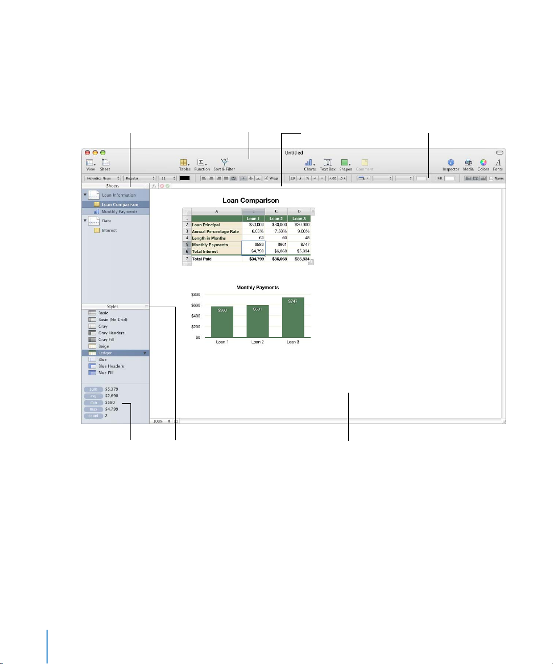
The Numbers Window

The Numbers window has elements that help you develop and organize your
spreadsheet.

Customize it to include the

The toolbar:

tools you use most often.

The Formula Bar:
Create and edit formulas
in table cells.

The Format Bar:
Quickly format the
selected object.

View the results of

calculations for values

in selected cells, and

drag calculations into

The Styles pane:
Select a predefined table style
to quickly format a table.

 Quickly add a new sheet by clicking the Sheet button in the toolbar. After you add

tables, charts, and other objects to a sheet, including imported graphics, movies, and
sound, you can drag objects around on the Numbers canvas to rearrange them.

 Use the Sheets pane to see a list of the tables and charts on any sheet.

 Apply predefined table styles listed in the Styles pane to change the appearance of a

selected table.

 Use the area in the lower left to perform instant calculations on values in selected

table cells.

20 Chapter 1 Numbers Tools and Techniques

The sheet canvas:

Create and edit tables, charts, and
other objects on a sheet.

 Use buttons in the toolbar to quickly add tables, charts, text boxes, media files, and

other objects.

For example, click the Tables button in the toolbar to add a new table that’s been
preformatted for the template you’re using. All templates contain several
preformatted tables for you to choose from.

See “The Toolbar” on page 24 to learn how to customize the toolbar so it includes
the tools you use most often.

 Use the Format Bar to quickly format a selected object.

 Use the Formula Bar to add and edit formulas in table cells.

Spreadsheet Viewing Aids

As you work on your spreadsheet, you may want to zoom in or out to get a better view
of what you are doing, or use other techniques for viewing the spreadsheet.

Zooming In or Out

You can enlarge (zoom in) or reduce (zoom out) your view of a sheet.

Here are ways to zoom in or out of a sheet:

m Choose View > Zoom > zoom level.

m Choose a magnification level from the pop-up menu at the bottom left of the canvas.

When you view a sheet in Print View, decrease the zoom level to view more pages in
the window at one time.

Click to show or hide a

sheet’s tables and charts.

The Sheets Pane

The Sheets pane is located along the top left side of the Numbers canvas. It lets you
quickly view and navigate to tables and charts in a sheet.

Click to add a new sheet.

Click a table or chart in
the list to select it and
show it in the window.

See “Using Sheets to Organize a Spreadsheet” on page 37 for more information.

Chapter 1 Numbers Tools and Techniques 21

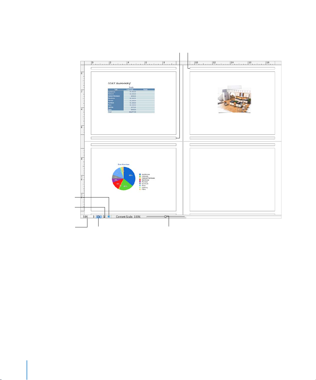
Print View

When you want to print a sheet or make a PDF of it, you can use Print View to visualize
the layout of objects on a sheet on individual pages.

Click to view pages in

landscape (horizontal)

orientation.

Click to view pages in

portrait (vertical)

orientation.

Click to choose a page

zoom level that lets you

see more or fewer pages.

Click to show or
hide Print View.

Footer area

Slide to shrink or enlarge all the
sheet’s objects.

Header area

See “Dividing a Sheet into Pages” on page 39 to learn more about Print View.

Alignment Guides

As you move objects around in a spreadsheet, alignment guides automatically appear
to help you position them on the page. See “Using Alignment Guides” on page 152 for
details about using alignment guides.

22 Chapter 1 Numbers Tools and Techniques

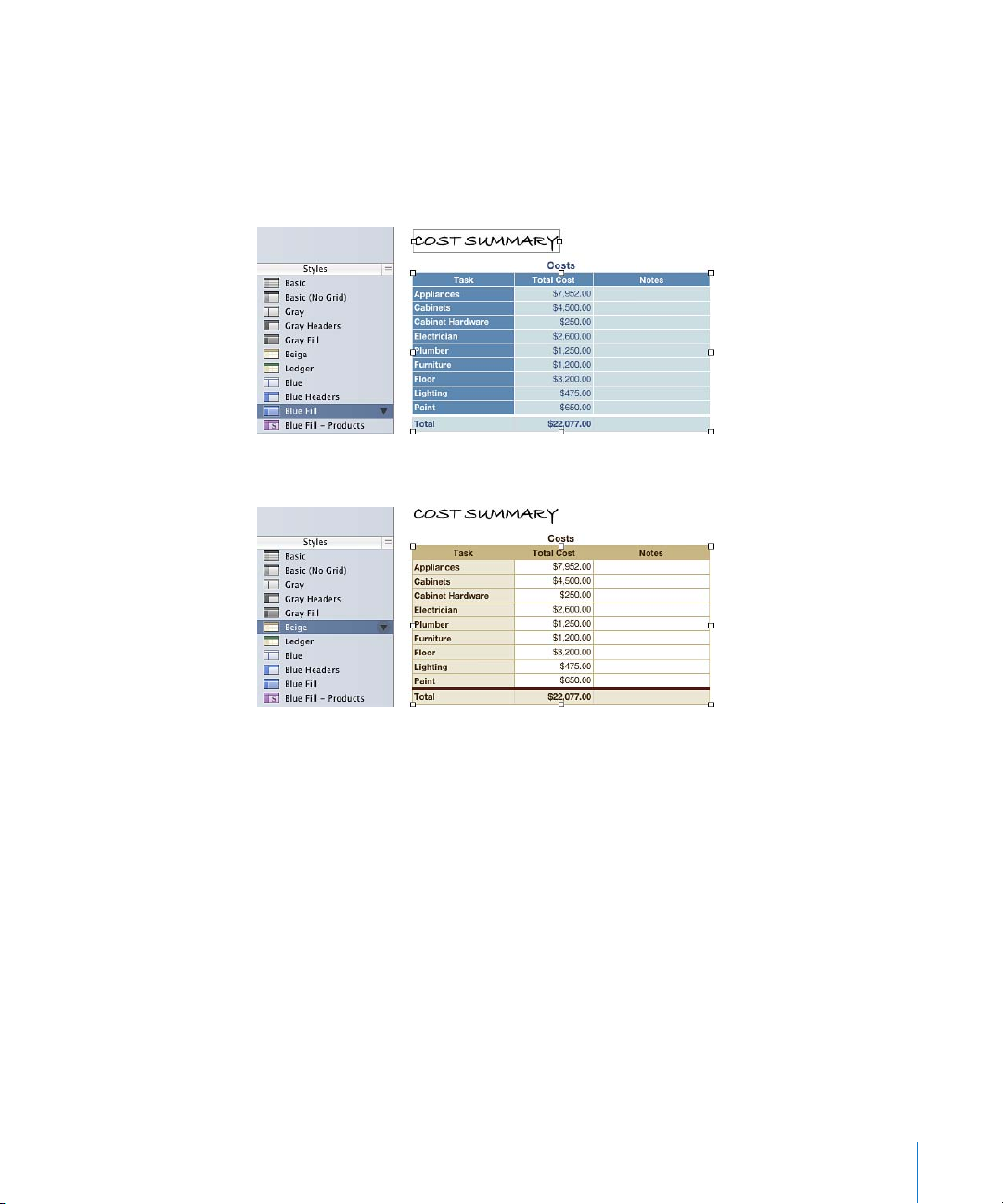
The Styles Pane

The styles pane lets you quickly apply predefined formatting to tables in a spreadsheet.
Table styles define such attributes as color, text size, and cell border formatting of table
cells.

To apply a table style, simply select the table and click a style in the Styles pane.

Switching from one table style to another takes only one click.

See “Using Table Styles” on page 79 for details.

Chapter 1 Numbers Tools and Techniques 23

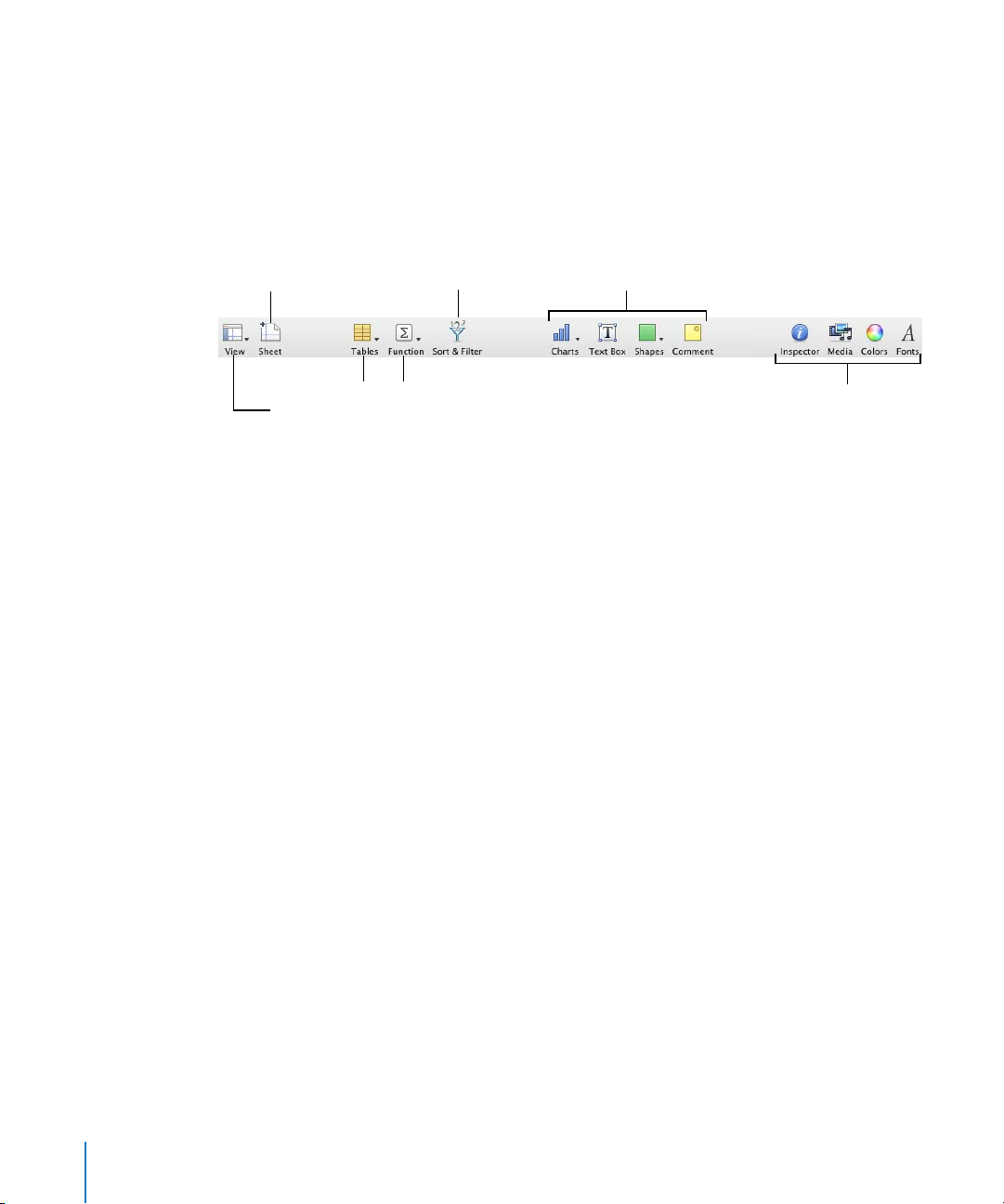
The Toolbar

The Numbers toolbar gives you one-click access to many of the actions you perform as
you work in Numbers. As you discover which actions you perform most often, you can
add, remove, and rearrange toolbar buttons to suit your working style.

To see a description of what a button does, hold your pointer over it.

The default set of toolbar buttons is shown below.

Add a chart, text box,

Add a sheet.

Sort and filter rows.

shape, or comment.

Add a table.

Show or hide Print View,
comments, and more.

Add a formula.

Open the Inspector window,

Media Browser, Colors

window, and Font panel.

To customize the toolbar:

1 Choose View > Customize Toolbar. The Customize Toolbar sheet appears.

2 Make changes to the toolbar as desired.

To add an item to the toolbar, drag its icon to the toolbar at the top. If you frequently
reconfigure the toolbar, you can add the Customize button to it.

To remove an item from the toolbar, drag it out of the toolbar.

To restore the default set of toolbar buttons, drag the default set to the toolbar.

To make the toolbar icons smaller, select Use Small Size.

To display only icons or only text, choose an option from the Show pop-up menu.

To rearrange items in the toolbar, drag them.

3 Click Done when you’ve finished.

You can perform several toolbar customization activities without using the Customize
Toolbar sheet:

 To remove an item from the toolbar, press the Command key while dragging the item

out of the toolbar.

You can also press the Control key while you click the item, and then choose Remove
Item from the shortcut menu.

 To move an item, press the Command key while dragging the item around in the

toolbar.

To show and hide the toolbar, choose View > Show Toolbar or View > Hide Toolbar.

24 Chapter 1 Numbers Tools and Techniques

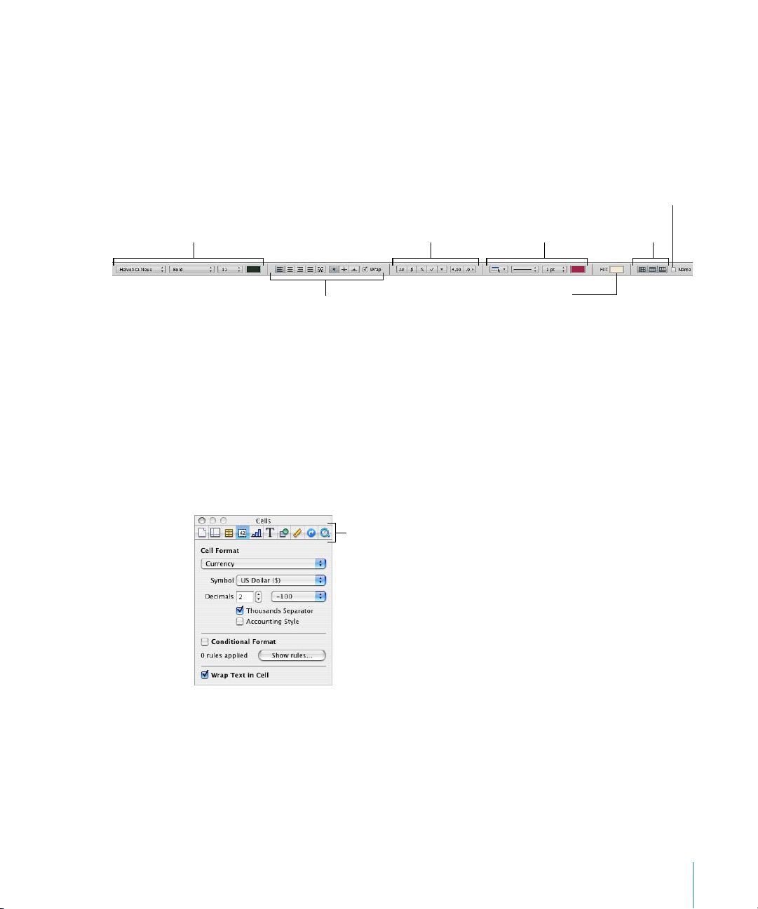
The Format Bar

Use the Format Bar, displayed beneath the toolbar, to quickly change the appearance
of tables, charts, text, and other elements in your spreadsheet.

The controls in the Format Bar vary with the object selected. To see a description of
what a Format Bar control does, hold the pointer over it.

Here’s what the Format Bar looks like when a table or table cell is selected.

Show or hide a table’s name.

Format text in table cells.

Format cell values.

Format cell borders.

Manage headers

and footer.

Arrange text in table cells.

Add background

color to a cell.

To show and hide the format bar:

m Choose View > Show Format Bar or View > Hide Format Bar.

The Inspector Window

Most elements of your spreadsheet can be formatted using the Numbers inspectors.
Each inspector focuses on a different aspect of formatting. For example, the Cells
Inspector lets you format cells and cell values. Hold your pointer over buttons and
other controls in the Inspector panes to see a description of what the controls do.

The buttons at the top of the
Inspector window open the ten
inspectors: Document, Sheet, Table,
Cells, Chart, Text, Graphics, Metrics,
Hyperlink, and QuickTime.

Opening multiple Inspector windows can make it easier to work on your spreadsheet.
For example, if you open both the Graphic Inspector and the Cells Inspector, you’ll have
access to all the image- and cell-formatting options.

Chapter 1 Numbers Tools and Techniques 25

Here are ways to open an Inspector window:

m Click Inspector in the toolbar.

m Choose View > Show Inspector.

m To open another Inspector window, press the Option key while clicking an Inspector

button.

After an Inspector window is open, click one of the buttons at the top to display a
different inspector. Clicking the second button from the left, for example, displays the
Sheet Inspector.

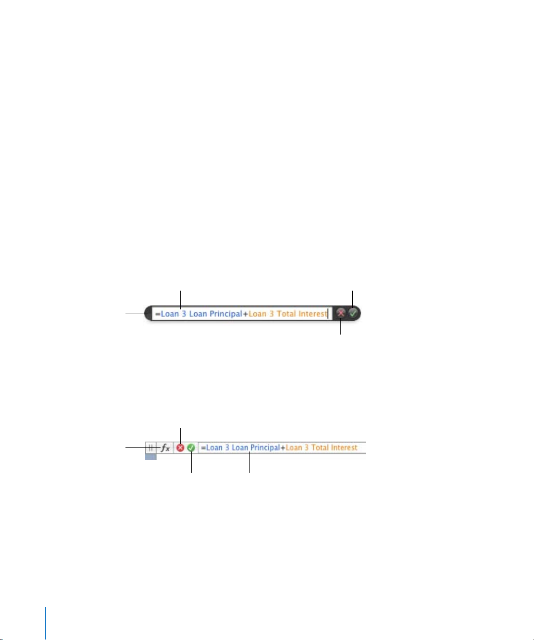
Formula Tools

You add a formula to a table cell when you want to display a value in the cell that’s
derived using a calculation. Numbers has several tools for working with formulas in
table cells:
 The Formula Editor lets you create and modify formulas. Open the Formula Editor by

selecting a table cell and typing the equal sign (=). You can also open it by choosing
Formula Editor from the Function pop-up menu in the toolbar.

Move the Formula Editor

by grabbing here

and dragging.

Click to open the

Function Browser.

Text field

View or edit a formula.

Accept button

Save changes.

Cancel button

Discard changes.

Learn more about this editor in “Using the Formula Editor” on page 88.

 The Formula Bar, always visible beneath the Format Bar, can also be used to create

and modify formulas.

Cancel button

Discard changes.

Accept button

Save changes.

Text field

View or edit a formula.

Instructions for adding and editing formulas using this tool are in “Using the Formula
Bar” on page 90.

26 Chapter 1 Numbers Tools and Techniques

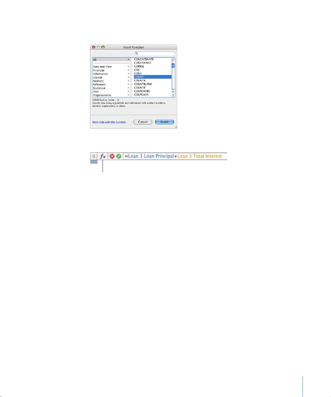
 Using the Function Browser is the fastest way to add a function. A function is a

predefined formula that has a name (such as SUM and AVERAGE).

To open the Function Browser, click the Function Browser button in the Formula Bar.

Click to open the
Function Browser.

“Using Functions” on page 96 tells you how to use the Function Browser.

Chapter 1 Numbers Tools and Techniques 27

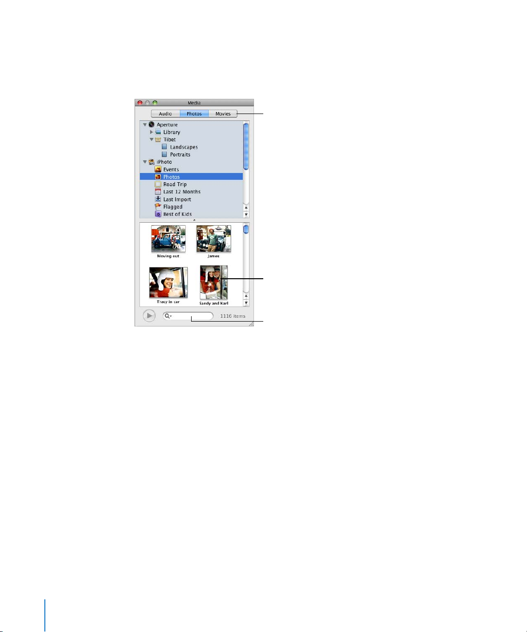
The Media Browser

The Media Browser provides access to all the media files in your iPhoto library, your
iTunes library, and your Movies folder. You can drag an item from the Media Browser to
your spreadsheet or to an image well in an inspector.

Click a button to view the files in
your iTunes library, your iPhoto
library, your Aperture library, or
your Movies folder.

Drag a file to your
spreadsheet.

Search for a file.

Here are ways to open the Media Browser:

m Click Media in the toolbar.

m Choose View > Show Media Browser.

The Colors Window

You use the Mac OS X Colors window to choose colors for text, table cells, cell borders,
and other objects. While you can also use the Format Bar to apply colors, the Colors
window offers advanced color management options.

To open the Colors window:

m Click Colors in the toolbar.

For more information, see “Using the Colors Window” on page 161.

28 Chapter 1 Numbers Tools and Techniques

The Font Panel

Using the Mac OS X Font panel, accessible from any application, you can change a
font’s typeface, size, and other options. Use the Format Bar for quick font formatting,
but use the Font panel for advanced font formatting.

To open the Font panel:

m Click Fonts in the toolbar.

For more detailed information about using the Font panel and changing the look of
text, see “Using the Font Panel to Format Text” on page 123.

The Warnings Window

When you import a document into Numbers, or export a Numbers spreadsheet to
another format, some elements might not transfer as expected. The Document
Warnings window lists any problems encountered.

If problems are encountered, you’ll see a message enabling you to review the warnings.
If you choose not to review them, you can see the Warnings window at any time by
choosing View > Show Document Warnings.

If you see a warning about a missing font, you can select the warning and click Replace
Font to choose a replacement font.

You can copy one or more warnings by selecting them in the Document Warnings
window and choosing Edit > Copy. You can then paste the copied text into an email
message, text file, or some other window.

Chapter 1 Numbers Tools and Techniques 29

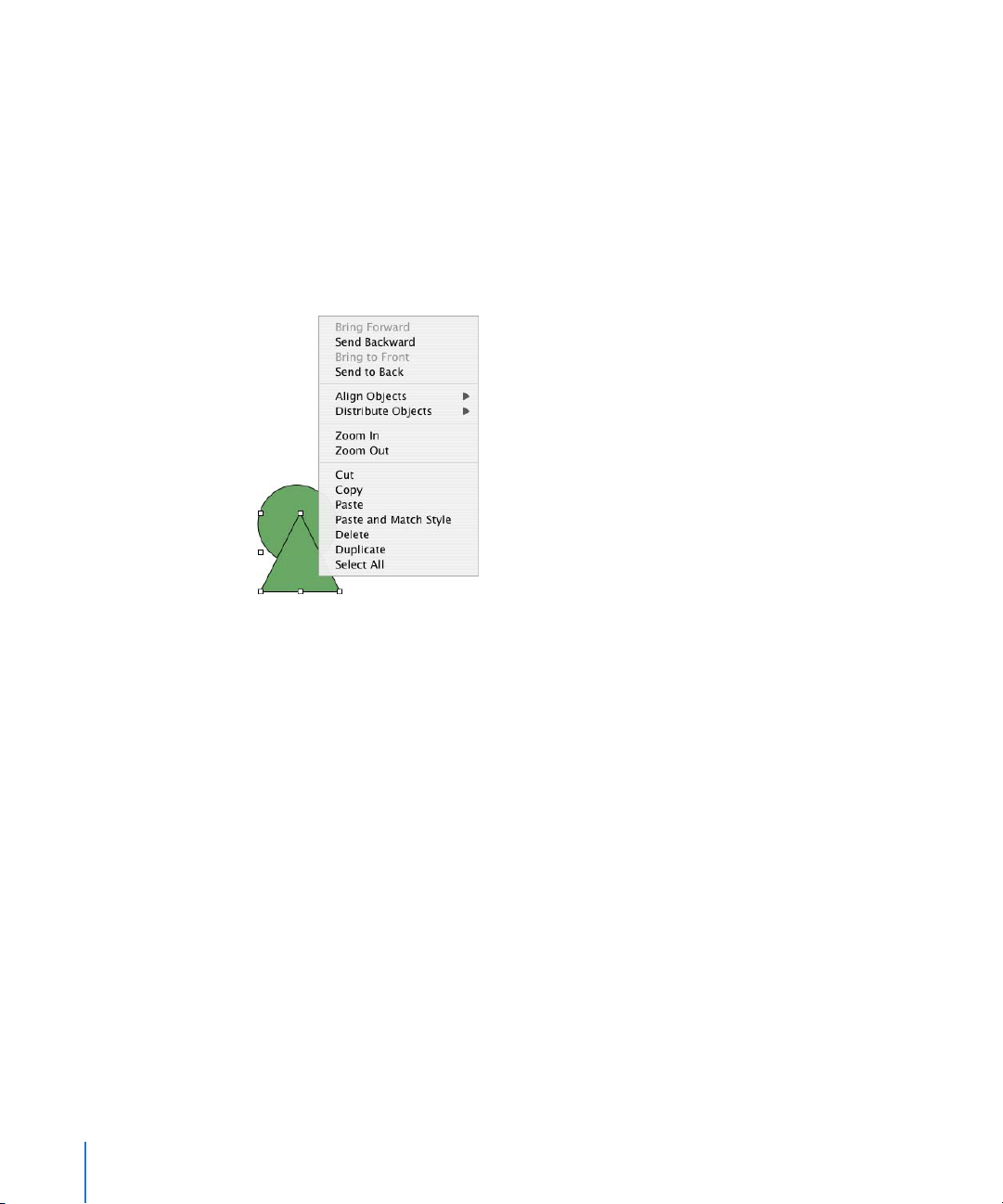
Keyboard Shortcuts and Shortcut Menus

You can use the keyboard to perform many of the Numbers menu commands and
tasks. To see a comprehensive list of keyboard shortcuts, open Numbers and choose
Help > Keyboard Shortcuts.

Many objects also have shortcut menus with commands you can use on the object.
Shortcut menus are especially useful for working with tables and charts.

To open a shortcut menu:

m Press the Control key while you click an object.

30 Chapter 1 Numbers Tools and Techniques

2 Working with a Numbers

Spreadsheet

2

This chapter describes how to manage Numbers
spreadsheets.

You can create a Numbers spreadsheet by opening Numbers and choosing a template.
You can also import a document created in another application, such as Microsoft Excel
or AppleWorks 6. This chapter tells you how to create new Numbers spreadsheets, as
well as how to open existing spreadsheets and save spreadsheets.

This chapter also provides instructions for using sheets and managing the layout of
printed or PDF versions of Numbers sheets.

Creating, Opening, and Importing Spreadsheets

When you create a new Numbers spreadsheet, you pick a template to provide its initial
format and content. You can also create a new Numbers spreadsheet by importing a
document created in another application, such as Microsoft Excel or AppleWorks.

Creating a New Spreadsheet

To create a new Numbers spreadsheet, you pick the template that provides appropriate
formatting and content characteristics.

Start with the Blank template to build your spreadsheet from scratch. Or select one of
the many other templates to create a budget, plan a party, and more without having to
do all the design work. Many templates include predefined tables, charts, and sample
data to give you a head start with your spreadsheet.

31

To create a new spreadsheet:

1 Open Numbers by clicking its icon in the Dock or by double-clicking its icon in the

Finder.

If Numbers is open, choose File > New from Template Chooser.

2 In the Template Chooser window, select a template category in the left column to

display related templates, and then select the template that best matches the
spreadsheet you want to create. If you want to begin in a spreadsheet without any
predefined content, select Blank.

3 Click Choose. A new spreadsheet opens on your screen.

To open a Blank template and bypass the Template Chooser window when you create a
new spreadsheet, select “Don’t show this dialog again.” To make the Template Chooser
reappear when you create a new spreadsheet, choose Numbers > Preferences, click
General, and then select “For New Documents: Show Template Chooser dialog.” Or you
can choose File > New from Template Chooser.

You can also have Numbers automatically open a particular template every time you
open Numbers or create a new spreadsheet. Choose Numbers > Preferences, click
General, select “For New Documents: Use template: template name,” and then click
Choose. Select a template name, and then click Choose.

32 Chapter 2 Working with a Numbers Spreadsheet

Importing a Document

You can create a new Numbers spreadsheet by importing a document created in
Microsoft Excel or AppleWorks 6. Numbers can also import files in comma-separated
value (CSV) format, tab-delimited format, and Open Financial Exchange (OFX) format.

From AppleWorks, you can only import spreadsheets.

Here are ways to import a document:

m Drag the document to the Numbers application icon. A new Numbers spreadsheet

opens, and the contents of the imported document are displayed.

m Choose File > Open, select the document, and then click Open.

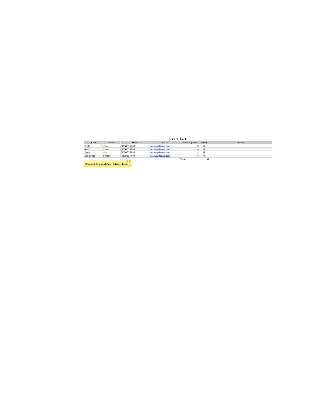
m You can import Address Book data to quickly create tables that contain names, phone

numbers, addresses, and other information for your contacts. See “Using Address Book
Fields” on page 179 for instructions.

If you can’t import a document, try opening the document in another application and
saving it in a format Numbers can read, or copy and paste the contents into an existing
Numbers spreadsheet.

You can also export Numbers spreadsheets to Microsoft Excel, PDF, and CSV files. See
“Exporting to Other Document Formats” on page 186 for details.

Opening an Existing Spreadsheet

There are several ways to open a spreadsheet that was created using Numbers.

Here are ways to open a spreadsheet:

m To open a spreadsheet when you’re working in Numbers, choose File > Open, select

the spreadsheet, and then click Open.

m To open a spreadsheet you’ve worked with recently, choose File > Open Recent and

choose the spreadsheet from the submenu.

m To open a Numbers spreadsheet from the Finder, double-click the spreadsheet icon or

drag it to the Numbers application icon.

If you see a message that a font or file is missing, you can still use the spreadsheet.
Numbers lets you choose fonts to substitute for missing fonts. Or you can add missing
fonts by quitting Numbers and adding the fonts to your Fonts folder (for more
information, see Mac Help). To make missing movies or sound files reappear, add them
to the spreadsheet again.

Chapter 2 Working with a Numbers Spreadsheet 33

Saving Spreadsheets

When you create a Numbers spreadsheet, all of the graphics are saved with the
spreadsheet so they display correctly if the spreadsheet is opened on another
computer. Fonts, however, are not included as part of the spreadsheet. If you transfer a
Numbers spreadsheet to another computer, make sure the fonts used in the
spreadsheet have been installed in the Fonts folder of that computer.

You can choose whether to save audio and movie files with a Numbers spreadsheet. If
you don’t save them with the spreadsheet, you need to transfer them separately to
view the spreadsheet on another computer.

Saving a Spreadsheet

It’s a good idea to save your spreadsheet often as you work. After you’ve saved it for
the first time, you can press Command-S to re-save it using the same settings.

To save a spreadsheet for the first time:

1 Choose File > Save, or press Command-S.

2 In the Save As field, type a name for the spreadsheet.

3 If your file directory isn’t visible in the Where pop-up menu, click the disclosure triangle

to the right of the Save As field.

4 Choose where you want to save the spreadsheet.

5 If you or someone else will open the spreadsheet on another computer, click Advanced

Options and set up options that determine what’s copied into your spreadsheet.

Copy audio and movies into document: Selecting this checkbox saves audio and video
files with the spreadsheet, so the files play if the spreadsheet is opened on another
computer. You might want to deselect this checkbox so that the file size is smaller, but
media files won’t play on another computer unless you transfer them as well.

Copy template images into document: If you don’t select this option and you open the
spreadsheet on a computer that doesn’t have Numbers installed, the spreadsheet
might look different.

6 Click Save.

You can generally save Numbers spreadsheets only to computers and servers that use
Mac OS X. Numbers is not compatible with Mac OS 9 computers and Windows servers
running Services for Macintosh. If you must use a Windows computer, try using AFP
server software available for Windows to do so.

If you plan to share the spreadsheet with others who don’t have Numbers installed on
their computers, you can export it for use in another application. To learn about
exporting your spreadsheet in other file formats, see “Exporting to Other Document
Formats” on page 186.

34 Chapter 2 Working with a Numbers Spreadsheet

You can also send a spreadsheet to iWeb. For more information, see “Sending a
Spreadsheet to iWeb” on page 187.

Undoing Changes

If you don’t want to save changes you made to your spreadsheet since opening it or
last saving it, you can undo them.

Here are ways to undo changes:

m To undo your most recent change, choose Edit > Undo.

m To undo multiple changes, choose Edit > Undo multiple times. You can undo any

changes you made since opening the spreadsheet or reverting to the last saved
version.

m To restore changes you’ve undone using Edit > Undo, choose Edit > Redo one or more

times.

m To undo all changes you made since the last time you saved your spreadsheet, choose

File > “Revert to Saved” and then click Revert.

Automatically Saving a Backup Version of a Spreadsheet

Each time you save a spreadsheet, you can save a copy without the changes you made
since last saving it. That way, if you change your mind about edits you have made, you
can go back to (revert to) the backup version of the spreadsheet.

Here are ways to create and use a backup version:

m To automatically save a backup version of a spreadsheet, choose Numbers >

Preferences, click General, and then select “Back up previous version when saving.”

The next time you save your spreadsheet, a backup version is created in the same
location, with “Backup of” preceding the filename. Only one version—the last saved
version—is backed up. Every time you save the spreadsheet, the old backup file is
replaced with the new backup file.

m To revert to the last saved version after making unsaved changes, choose File > Revert

to Saved. The changes in your open spreadsheet are undone.

Saving a Spreadsheet as a Template

When you save a spreadsheet as a template, it appears in the Template Chooser.

To save a spreadsheet as a template:

m Choose File > Save as Template.

See “Designing a Template” on page 188 for additional details.

Chapter 2 Working with a Numbers Spreadsheet 35

Saving Search Terms for a Spreadsheet

You can store such information as author name and keywords in Numbers
spreadsheets, and then use Spotlight to locate spreadsheets containing that
information.

To store information about a spreadsheet:

1 Click Inspector in the toolbar, and then click the Document Inspector button.

2 In the Spotlight fields, enter or change information.

To search for spreadsheets containing Spotlight information, click the Spotlight icon at
the top right of the menu bar, and then type what you want to search for.

Saving a Copy of a Spreadsheet

If you want to make a copy of your spreadsheet (for example, to create a backup copy
or multiple versions), you can save it using a different name or location. (You can also
automate saving a backup version, as “Automatically Saving a Backup Version of a
Spreadsheet” describes.)

To save a copy of a spreadsheet:

m Choose File > Save As and specify a name and location.

The spreadsheet with the new name remains open. To work with the previous version,
choose File > Open Recent and choose the previous version from the submenu.

Closing a Spreadsheet Without Quitting Numbers

When you have finished working with a spreadsheet, you can close it without quitting
Numbers.

To close the active spreadsheet and keep the application open:

m Choose File > Close or click the close button in the upper-left corner of the Numbers

window.

36 Chapter 2 Working with a Numbers Spreadsheet

Click to show or hide a

sheet’s tables and charts.

If you’ve made changes since you last saved the spreadsheet, Numbers prompts you to
save.

Using Sheets to Organize a Spreadsheet

Like chapters in a book, sheets let you divide information into manageable groups. For
example, you might want to place charts in the same sheet as the tables whose data
they display. Or you may want to place all the tables on one sheet and all the charts on
another sheet. You might want to use one sheet for keeping track of business contacts
and other sheets for friends and relatives.

The sheets in a spreadsheet and the tables and charts on each sheet are represented in
the Sheets pane, located to the left of the canvas above the styles pane.

Click to add a new sheet.

Only tables and charts are listed for any sheet, even if you have text, images, and other
objects in your spreadsheet.

The order of a sheet’s tables and charts in the Sheets pane may not match their order
in the spreadsheet, as “Reorganizing Sheets and Their Contents” on page 38 describes.

Viewing Sheets

The Sheets pane on the left of the Numbers window lists all the sheets in your
spreadsheet and the tables and charts in each sheet.

Here are ways to see a sheet’s tables and charts:

m To show or hide all a sheet’s tables and charts in the Sheets pane, click the triangle to

the left of the sheet in the pane.

m To display the contents of a sheet, click the sheet in the Sheets pane.

When you’re working on a table or chart in the spreadsheet, the table or chart is
highlighted in the Sheets pane.

Chapter 2 Working with a Numbers Spreadsheet 37

Adding and Deleting Sheets

There are several ways to add and delete sheets.

Here are ways to create and remove sheets:

m To add a new sheet, click the Sheet button in the toolbar. You can also choose Insert >

Sheet.

A new sheet containing a predefined table is added at the bottom of the Sheets pane.
You can move the sheet by dragging it to a new location in the Sheets pane.

m To add a sheet that’s a copy of a sheet in the spreadsheet, select the sheet to copy,

choose Edit > Copy, select the sheet after which you want the copy located, and
choose Edit > Paste.

m To delete a sheet and its contents, select it in the Sheets pane and press the Delete key.

When you add a sheet, Numbers assigns it a default name, but you can change the
name, as “Changing Sheet Names” on page 39 describes.

Reorganizing Sheets and Their Contents

In the Sheets pane, you can move sheets around and reorder their tables and charts.
You can also move tables and charts from one sheet to another.

Reordering tables and charts in the Sheets pane doesn’t affect their location in a sheet.
In a sheet in the Sheets pane, for example, you may want to place charts next to the
tables they’re derived from, or list tables in the order in which you want to work on
them. But in the sheet itself, you may want to present these objects in a different order
(for example, when you lay out your spreadsheet for printing).

Here are ways to reorganize sheets in the Sheets pane:

m To move a sheet, select it and drag it to a new location in the pane. Sheets shift to

make room for your insertion as you drag.

You can also select multiple sheets and move them as a group.

m To copy (or cut) and paste sheets, select the sheets, choose Edit > Cut or Edit > Copy,

select the sheet after which you want to place the sheets you’re moving, and choose
Edit > Paste.

m To move one or more tables and charts associated with a sheet, select them and drag

them to a new location in the same sheet or to a different sheet.

You can also use cut/paste or copy/paste actions to move tables and charts in the
pane.

To move an object within a sheet in the spreadsheet, select it and drag it to a different
location, or use cut/paste or copy/paste actions. To place objects on specific pages,
follow the instructions in “Dividing a Sheet into Pages” on page 39.

38 Chapter 2 Working with a Numbers Spreadsheet

Changing Sheet Names

A name distinguishes each sheet in the Sheets pane. The sheet name is assigned by
default when you add a sheet, but you can change it to a more descriptive name.

Here are ways to change a sheet’s name:

m In the Sheets pane, double-click the name and edit it.

m In the Sheet Inspector, edit the name in the Name field.

You can also change the names of a sheet’s tables and charts. See “Naming Tables” on
page 49 and “Using a Chart Title” on page 107 for instructions.

Dividing a Sheet into Pages

Using Print View, you can view a sheet as individual pages, moving and resizing objects
until you achieve the layout you want for a printed or PDF version of the sheet. You can
also add headers, footers, page numbers, and more.

Click to view pages in

landscape (horizontal)

orientation.

Click to view pages in

portrait (vertical)

orientation.

Click to choose a page

zoom level that lets you

see more or fewer pages.

Click to show or
hide Print View.

Footer area

Slide to shrink or enlarge all the
sheet’s objects.

Header area

Chapter 2 Working with a Numbers Spreadsheet 39

Here are ways to show or hide Print View:

m Click View in the toolbar, and then choose Show Print View or Hide Print View.

m Choose File > Show Print View, View > Show Print View, File > Hide Print View, or

View > Hide Print View.

m Click the page icon next to the page zoom control in the lower left of the canvas.

When you use Print View, the zoom level you choose from the pop-up menu in the
lower left determines how many pages you can view in the window at one time.

You set up page attributes, such as page orientation and margins, separately for each
sheet, using the Sheet Inspector.

Type a name for the sheet.

Shrink or enlarge all the sheet’s objects.

Set the page orientation and
pagination order.

Specify the sheet’s starting page number.

Set page margins.

Setting a Spreadsheet’s Page Size

Before working with Print View, set the size of the pages to reflect the size of the paper
you’ll be using.

To set the page size:

1 Click Inspector in the toolbar, and then click the Document Inspector button.

2 Choose a page size from the Paper Size pop-up menu.

40 Chapter 2 Working with a Numbers Spreadsheet

Using Headers and Footers

You can have the same text appear on multiple pages in a sheet. Recurring information
that appears at the top of the page is called a header; at the bottom it’s called a footer.

You can put your own text in a header or footer, and you can use formatted text fields.
Formatted text fields allow you to insert text that is automatically updated. For
example, inserting the date field shows the current date whenever you open the
spreadsheet. Similarly, page number fields keep track of page numbers as you add or
delete pages.

To define the contents of a header or footer:

1 Click View in the toolbar and choose Show Print View.

2 To see header and footer areas, hover the pointer near the top or bottom of a page.

You can also click View in the toolbar and choose Show Layout.

3 To add text to a header or footer, place the insertion point in the header or footer and

insert text.

4 To add page numbers or other changeable values, see the instructions in “Inserting

Page Numbers and Other Changeable Values” on page 145.

Arranging Objects on a Page

Resize objects, move them around on a page or between pages, and break up long
tables across pages when you’re viewing a sheet in Print View.

To show Print View, click View in the toolbar and choose Show Print View.

Here are ways to lay out objects on a selected sheet’s pages:

m To adjust the size of all the objects in the sheet in order to change the number of

pages they occupy, use the Content Scale controls in the Sheet Inspector.

You can also drag the Content Scale slider at the bottom left of the canvas to resize
everything on a sheet.

m To resize individual objects, select them and drag their selection handles or change the

Size field values in the Metrics Inspector.

To resize a table, see “Resizing a Table” on page 48. To resize a chart, see “Resizing a
Chart” on page 107. To resize other objects, see “Resizing Objects” on page 154.

m Header rows and header columns can be set to appear on each page if a table spans

more than one page by selecting “Repeat header cells on each page” in the Table
Inspector. You can also choose Table > Repeat Header Rows or Table > Repeat Header
Columns.

Chapter 2 Working with a Numbers Spreadsheet 41

To avoid showing header rows or columns when a table spans pages, deselect “Repeat
header cells on each page” in the Table Inspector or choose Table > Don’t Repeat
Header Rows or Table > Don’t Repeat Header Columns.

m Move objects from page to page by dragging them or by cutting and pasting them.

Setting Page Orientation

You can lay out pages in a sheet in a vertical orientation (portrait) or a horizontal
orientation (landscape).

To set a sheet’s page orientation:

1 Click View in the toolbar and choose Show Print View.

2 Click Inspector in the toolbar, click the Sheet Inspector button, and click the

appropriate page orientation button in the Page Layout area of the pane.

You can also click a page orientation button at the bottom left of the canvas.

Setting Pagination Order

You can order pages viewed in page mode from left to right or from top to bottom
when you print them or create a PDF.

To set pagination order:

m Click Inspector in the toolbar, click the Sheet Inspector button, and then click the top-

to-bottom or left-to-right button in the Page Layout area of the pane.

Numbering Pages

You can display page numbers in a page’s header or footer.

To number a sheet’s pages:

1 Select the sheet.

2 Click View in the toolbar and choose Show Print View.

3 Click View in the toolbar and choose Show Layout so you can see the headers and

footers.

You can also see the headers and footers by hovering the pointer over the top or
bottom of a page.

4 Click into the first header or footer to add a page number, following the instructions in

“Inserting Page Numbers and Other Changeable Values” on page 145.

5 Click Inspector in the toolbar, click the Sheet Inspector button, and then specify the

starting page number.

To continue page numbers from the previously selected sheet, select “Continue from
previous sheet.”

To start the sheet’s page numbers at a particular number, use the Start At field.

42 Chapter 2 Working with a Numbers Spreadsheet

Setting Page Margins

In Print View, every sheet’s page has margins (blank space between the sheet’s edge
and the edges of the paper). These margins are indicated onscreen by light gray lines,
visible when you use layout view.

To set the page margins for a sheet:

1 Select the sheet in the Sheets pane.

2 Click View in the toolbar and choose Show Print View and Show Layout.

3 Click Inspector in the toolbar, and then click the Sheet Inspector button.

4 To set the distance between the layout margins and the left, right, top, and bottom

sides of a page, enter values in the Left, Right, Top, and Bottom fields.

5 To set the distance between a header or a footer and the top or bottom edge of the

page, enter values in the Header and Footer fields.

To print the spreadsheet using the largest printing area possible with any printer you
use, select Use Printer Margins. Any margin settings specified in the Sheet Inspector will
be ignored when you print.

Chapter 2 Working with a Numbers Spreadsheet 43

3 Using Tables

This chapter tells you how to add and format tables and
cell values.

Several other chapters provide instructions that focus on particular aspects of tables:

 To learn about using styles to format tables, see Chapter 4, “Working with Table

Styles,” on page 79.

 To learn about using formulas in table cells, see Chapter 5, “Using Formulas and

Functions in Tables,” on page 83.

 To learn about displaying table values in charts, see Chapter 6, “Using Charts,” on

page 98.

About Tables

Tables help you organize, analyze, and present data.

3

44

Numbers provides a wide variety of options for building and formatting tables and
handling values of different types. You can also use special operations such as sorting
and conditional formatting (a technique for automating the monitoring of cell values).

 “Working with Tables” on page 45 teaches you how to add tables, resize them, move

them, name them, and more.

 “Selecting Tables and Their Components” on page 51 describes how to select tables,

columns, and other table elements in order to work with them.

 “Working with Content in Table Cells” on page 54 tells you how to add text, numbers,

dates, images, and other content to table cells as well as how to monitor cell values
automatically.

 “Working with Rows and Columns” on page 69 covers adding rows and columns,

resizing them, and more.

 “Working with Table Cells” on page 74 contains instructions for splitting cells,

merging them, and copying and moving them as well as formatting cell borders.

 “Reorganizing Tables” on page 77 describes how to sort and filter rows.

Working with Tables

Use a variety of techniques to create tables and manage their characteristics, size, and
location.

Adding a Table

While most templates contain one or more predefined tables, you can add additional
tables to your Numbers spreadsheet.

Here are ways to add a table:

m Click Tables in the toolbar and choose a predefined table from the pop-up menu.

You can add your own predefined tables to the pop-up menu. See “Defining Reusable
Tables” on page 49 for instructions.

m Choose Insert > Table > table.

m To create a new table based on one cell or several adjacent cells in an existing table,

select the cell or cells, click and hold the selection, and then drag the selection to the
sheet. To retain values in the selected cells in the original table, hold down the Option
key while dragging.

See “Selecting Tables and Their Components” on page 51 to learn about cell selection
techniques.

m To create a new table based on an entire row or column in an existing table, click the

reference tab associated with the row or column, click and hold the reference tab, drag
the row or column to the sheet, and then release the tab. To retain values in the
column or row in the original table, hold down the Option key while dragging.

Using Table Tools

You can format a table and its columns, rows, cells, and cell values using various
Numbers tools.

Here are ways to manage table characteristics:

m Select a table and use the Format Bar to quickly format the table.

Show or hide a table’s name.

Format text in table cells.

Chapter 3 Using Tables 45

Format cell values.

Arrange text in table cells.

Format cell borders.

Add background

color to a cell.

Manage headers

and footer.

m Use the Table Inspector to access table-specific controls, such as fields for precisely

controlling column width and row height. To open the Table Inspector, click Inspector
in the toolbar, and click the Table Inspector button.

Add a table name.

Add and remove a header row, a header
column, and a footer row.

Merge or split selected cells.

Adjust the size of rows and columns.

Set the style, width, and color of
cell borders.

Add color or an image to a cell.

Change the behavior of the Return and
Tab keys. See “Selecting a Table Cell”

Control the visibility of header
cells in multipage tables.

on page 51 for details.

m Use the Cells Inspector to format cell values. For example, you can display a currency

symbol in cells containing monetary values.

You can also set up conditional formatting. For example, you can make a cell red when
its value exceeds a particular number.

To open the Cells Inspector, click Inspector in the toolbar, and click the Cells Inspector
button.

46 Chapter 3 Using Tables

Set up the format for displaying
values in selected cells.

Use color to highlight cells
whose values obey your rules.

Select to wrap text in selected cells.

m Use table styles to adjust the appearance of tables quickly and consistently. See “Using

Table Styles” on page 79 for more information.

m Use the reference tabs and handles that appear when you select a table cell to quickly

reorganize a table, select all the cells in a row or column, add or delete rows and
columns, and more.

Drag the Table handle
to move the table.

Click the Row handle to add one row.
Drag it to add more rows.

Reference tab numbers can
be used to refer to rows.

Reference tab letters can be
used to refer to columns.

Click the Column handle to
add one column. Drag it to
add multiple columns.

Drag the Column and Row
handle down to add rows. Drag it
to the right to add columns.

You also use reference tabs when you work with formulas (“Using Cell References” on
page 91 tells you how).

m Use the Graphics Inspector to create special visual effects, such as shadows. To open

the Graphics Inspector, click Inspector in the toolbar and then click the Graphics
Inspector button.

m Access a shortcut menu by selecting a table or cell(s) and then holding down the

Control key as you click again.

You can also use the pop-up menus on the column and row reference tabs.

m Use the Formula Editor and Formula Bar to add and edit formulas. See “Using the

Formula Editor” on page 88 and “Using the Formula Bar” on page 90 for details.

m Use the Formula Browser to add and edit functions. See “Using Functions” on page 96

for details.

Chapter 3 Using Tables 47

Resizing a Table

You can make a table larger or smaller by dragging one of its selection handles or by
using the Metrics Inspector. You can also change the size of a table by resizing its
columns and rows.

Here are ways to resize a table that’s selected:

m Drag one of the square selection handles that appear when a table is selected. See

“Selecting a Table” on page 51 for instructions.

To maintain a table's proportions, hold down the Shift key as you drag to resize the
table.

To resize from the table’s center, hold down the Option key as you drag.

To resize a table in one direction, drag a side handle instead of a corner handle.

m To resize by specifying exact dimensions, select a table or table cell, click Inspector in

the toolbar, and then click the Metrics Inspector button. Using the Metrics Inspector,
you can specify a new width and height, and you can change the table’s distance from
the margins by using the Position fields.

m If a table spans more than one page, you must use the Metrics Inspector to resize the

table. To resize by adjusting the dimensions of rows and columns, see “Resizing Table
Rows and Columns” on page 73.

Moving Tables

You can move a table by dragging it, or you can relocate a table using the Metrics
Inspector.

Here are ways to move a table:

m If the table isn’t selected, click and hold at the edge of the table, and drag the table.

If the table is selected, drag the table while holding down the Table handle in the
upper left.

m To constrain the movement to horizontal, vertical, or 45 degrees, hold down the Shift

key as you drag.

48 Chapter 3 Using Tables

m To move a table more precisely, click any cell, click Inspector in the toolbar, click the

Metrics Inspector button, and then use the Position fields to relocate the table.

m To copy a table and move the copy, hold down the Option key, click and hold at the

edge of an unselected table, and drag.

Naming Tables

Every Numbers table has a name that’s displayed in the Sheets pane and can optionally
be displayed above the table. The default table name (Table 1, Table 2, and so forth)
can be changed, hidden, and formatted, but not moved or resized.

Here are ways to work with table names:

m To change the name, edit it in the Sheets pane or in the Table Inspector’s Name field.

On any sheet, two tables can’t have the same name.

m To show the table name on the sheet, select Name in the Format Bar or the Table

Inspector.

To hide the table name on the sheet, deselect Name.

m To format the name, make sure the table isn’t selected, select Name in the Format Bar

or the Table Inspector, click the table name to select the name region on the sheet, and
use the Format Bar, Font panel, or Text pane of the Text Inspector.

m To increase the distance between the table name and the table body, select Name in

the Table Inspector, click the name on the canvas, and then use the Text Inspector to
modify the After Paragraph value.

Defining Reusable Tables

You can add your own tables to the menu of predefined tables that appears when you
click Tables in the toolbar or choose Insert > Table. Reusable tables have the table style
and geometry of your choice and can contain content (header text, formulas, and so
forth).

To define a reusable table:

1 Select a table.

2 Define a table style for the table. The table style determines the formatting of borders,

background, and text in the table’s cells.

One way to define the table style is by following the instructions in “Modifying a Table’s
Style” on page 80.

Alternatively, you can use the default table style that’s in effect when you add a table to
the spreadsheet that’s based on the reusable table. (See “Using the Default Table Style”
on page 81 to learn about the default table style.) Step 7 tells you how to use this
option.

Chapter 3 Using Tables 49

3 Define the table’s geometry.

To resize the table, see “Resizing a Table” on page 48 and “Resizing Table Rows and
Columns” on page 73.

To define columns and rows, see “Working with Rows and Columns” on page 69.

To split or merge, and resize table cells, see “Splitting Table Cells” on page 74 or
“Merging Table Cells” on page 74.

4 Add and format any content you want to reuse. See “Working with Content in Table

Cells” on page 54 for instructions. Any formulas you add should refer only to cells in the
table you’re defining.

5 Choose Format > Advanced > Capture Table.

6 Type a name for the table.

7 Select “Use the default style from the document” if you want the table to be styled

using the default table style in effect when the table is added to the spreadsheet.
Otherwise the table style used is the one you defined in step 2.

8 Click OK.

A copy of your reusable table can now be added to the current spreadsheet by
choosing it from the menu of predefined tables that appears when you click Tables in
the toolbar or choose Insert > Table.

To rearrange, rename, or delete tables on the menu, choose Format > Advanced >
Manage Tables. Double-click a name to change the name of a predefined table. Select a
table and click the up or down arrow buttons to move it up or down in the list of
tables. Click the Delete (–) button to remove a table. Click Done when you’ve finished.

The table and menu changes apply only to the current spreadsheet. If you want your
reusable tables and menu changes to be available in other spreadsheets, save the
spreadsheet as a template, using the instructions in “Designing a Template” on
page 188.

Copying Tables Among iWork Applications

You can copy a table from one iWork application to another.

The table retains its appearance, data, and other attributes, but some Numbers features
aren’t supported in the other applications:

 Rows or columns that are hidden in Numbers aren’t visible in the other applications

until you select the table and choose Format > Table > Unhide All Rows or Unhide All
Columns.

 Comments added to Numbers table cells aren’t copied.

50 Chapter 3 Using Tables

To copy a table from one iWork application to another:

1 Select the table you want to copy, as “Selecting a Table” on page 51 describes.

2 Choose Edit > Copy.

3 In the other application, set an insertion point for the copied table, and then choose

Edit > Paste.

Selecting Tables and Their Components

You select tables, rows, columns, table cells, and table cell borders before you work
with them.

Selecting a Table

When you select a table, selection handles appear on the edges of the table.

Here are ways to select a table:

m If the table cell isn’t selected, move your pointer to the edge of the table. When the

pointer changes to include a black cross, and you can click to select the table.

m If a table cell or border segment is selected, click the Table handle in the upper left to

select the table. You can also press Command-Return.

Selecting a Table Cell

When you select a cell, the border of the selected cell is highlighted.

Selecting a cell also displays reference tabs along the top and sides of the table.

To select a single table cell:

1 Move the pointer over the cell. The pointer changes into a white cross.

2 Click the cell.

Chapter 3 Using Tables 51

When a cell is selected, use the Tab, Return, and arrow keys to move the selection to an
adjacent cell. Selecting “Return key moves to next cell” under Table Options in the Table
Inspector sometimes changes the effect of the Return and Tab keys.

If “Return key” option is

To select

The next cell to the right Press Tab.

The previous cell Press Shift-Tab. Press Shift-Tab.

The next cell down Press Down Arrow or Return.

The next cell up Press Up Arrow or Shift-Return. Press Up Arrow.

selected

If you press Tab when the last
cell in a column is selected, a
new column is added.

If you add or change data in the
last column, press Tab twice to
add a new column.

If you’ve been using the Tab key
to navigate between cells,
pressing Return selects the next
cell down from the cell in which
you started tabbing.

If you press Return when the last
cell in a row is selected, a new
row is added.

If you add or change data in the
last cell, press Return twice to
add a new row.

If “Return key” option isn’t
selected

Press Tab.
If you press Tab in the last

column, the first cell in the next
row is selected.

If you press Tab in the last cell of
the table, a new row is added.

If you press Shift-Tab in the first
cell, the last cell is selected.

Press Down Arrow.

Selecting a Group of Table Cells

You can select adjacent or nonadjacent cells.

Here are ways to select a group of cells:

m To select adjacent table cells, select a single cell, and then hold down the Shift key as

you select adjacent cells.

You can also click a cell, hold it, and then drag through a range of cells.

m To select nonadjacent table cells, hold down the Command key as you select cells. Use

Command-click to deselect a cell in the group.

Selecting a Row or Column

Select rows and columns using their reference tabs.

52 Chapter 3 Using Tables

To select an entire row or column:

1 Select any table cell so that the reference tabs are showing.

2 To select a column, click its reference tab (above the column).

To select a row, click its reference tab (to the left of the row).

Selecting Table Cell Borders

Select cell border segments when you want to format them. A single border segment is
one side of a cell. A long border segment includes all adjacent single border segments.

A single (horizontal)
border segment

A single (vertical) border
segment

A long (vertical) border
segment

A long (horizontal)
border segment

Here are ways to select border segments:

m To select border segments in a single step, select a table, row, column, or cell.

Click the Borders button in the Format Bar, and choose an option from the pop-up
menu.

Borders button

Chapter 3 Using Tables 53

You can also use the Cell Borders buttons in the Table Inspector to select a border
segment.

m To select and deselect segments by clicking them in a table, use border selection

mode. Choose Allow Border Selection from the Borders pop-up menu in the Format Bar
or choose Table > Allow Border Selection, and then select the table you want to work
with.

The pointer changes shape when it’s over a horizontal or vertical segment. The pointer
appears to straddle the segment.

The pointer looks like this when
it’s over a horizontal segment.

The pointer looks like this when
it’s over a vertical segment.

To select a long segment, click a cell’s horizontal or vertical border. To change the
selection to a single segment, click it again.

Click to go back and forth between single-segment and long-segment selection.

To add a single or long segment to the selection, hold down the Shift or Command key
while clicking.

To deselect a selected single segment, click it while holding down the Shift or
Command key.

To stop using border selection mode, choose Disallow Border Selection from the
Borders pop-up menu in the Format Bar or choose Table > Disallow Border Selection.

Working with Content in Table Cells

You can add text, numbers, and dates to table cells, and you can format values in cells.
You can also add images and background color, as well as checkboxes, sliders, and
other controls. And you can use autofilling to use the content in one or more cells to
automatically add values to adjacent cells.

Adding and Editing Cell Values

You can add, change, and delete the content in cells.

Here are ways to add and edit values:

m If the cell is empty, select it and then type a value. “Selecting a Table Cell” on page 51

tells you how to select cells.

m To replace specific content already in the cell, select the cell and then select what you

want to replace by double-clicking; hold down the Shift key and select more content if
you want to replace more. Type to replace the selected content.

54 Chapter 3 Using Tables

m To replace everything in the cell, select the cell and then begin typing.

If “Return key moves to next cell” isn’t selected in the Table Inspector, you can also
select the cell and then press Return or Enter, which selects everything in the cell, and
then start typing.

m To insert content within existing content, select the cell, click to set the insertion point,

and begin typing.

m To undo changes made to a table cell since selecting the cell, press Esc.

m To delete the content of table cells, rows, or columns, select the cells, rows, or columns

and then press the Delete key or choose Edit > Delete.

To delete the contents, background fill, and any style settings, choose Edit > Clear All.
The default style is applied to the selection.

m To copy, paste, and move cell values, see the instructions in “Copying and Moving Cells”

on page 76.

m To add formulas and functions to cells, see the instructions in “Using Formulas” on

page 83 and “Using Functions” on page 96.

Working with Text in Cells

You can control the format and alignment of text in table cells, and you can use find/
replace and spell-checking features.

When you type text into a cell, Numbers displays text that might be used to complete
the cell content based on similar text elsewhere in the table. You can use the suggested
text if it’s appropriate, or you can keep typing to override suggestions.

Here are techniques for working with text in table cells:

m To insert a line break, press Control-Return.

m To insert a paragraph break, If “Return key moves to next cell” under Table Options in

the Table Inspector isn’t selected, press Return. Otherwise, press Option-Return.

m To insert a tab in a table, press Option-Tab.

m To adjust text alignment, use the alignment buttons in the Format Bar.

Align text to the top, middle,
or bottom of cells.

Align text to the left, center, right; justify text; or
align text to the left and numbers to the right.

The Text Inspector gives you additional text formatting options (click Inspector in the
toolbar and click the Text Inspector button).

Chapter 3 Using Tables 55

m To control font attributes, use the text formatting buttons in the Format Bar.

Choose a typeface.

Choose the text color.

Choose a font.

Choose the font size.

You can also use the Font panel (click Fonts in the toolbar).

m To check spelling, follow the instructions in “Checking for Spelling Mistakes” on

page 146.

m To find and optionally replace text in cells, follow the instructions in “Finding and

Replacing Text” on page 148.

m To avoid having Numbers interpret what you type as a number, use the text format.

See “Using the Text Format” on page 64 for details.

Note: Text strings are ignored in functions that use values to perform calculations.

Working with Numbers in Cells

Some table operations, such as formulas and functions that perform mathematical
operations, depend on cells containing numeric values.

Here are techniques for working with numbers in table cells:

m In a numeric cell use only numbers (0 through 9) or one of the following characters: +,

–, (, ), /, $, %, a period, E, or e.

m You can type some characters (such as %) into a cell, or you can use a cell format, as

“Formatting Cell Values” on page 58 describes.

m To specify a negative number, precede it with the minus sign (–).

When you put a number in a table cell that’s too large to display, Numbers converts the
number:

 When a decimal number doesn’t fit in a cell, the number is rounded. For example,

1.77777777777777777777 becomes 1.77777777777778.

 When a whole number doesn’t fit in a cell, the number is displayed using scientific

notation. For example, 77777777777777777777 becomes 7.7.77778E+19.

Scientific notation displays numbers using an exponent raised by the power of 10.
The exponent is displayed following the E.

If the converted number still doesn’t fit, it’s clipped. See “Displaying Content Too Large
for Its Cell” on page 57 for suggestions.

Instructions for using formulas and functions in table cells are in “Using Formulas” on
page 83 and “Using Functions” on page 96.

56 Chapter 3 Using Tables

Working with Dates in Cells

Unless a cell has a date and time format associated with it, when you type a value that
can be interpreted as a date or time value, Numbers might reformat the value.

For example, if you type 1/22/45 or 1-22-45 into a table cell with the Automatic cell
format and leave the cell, the value changes to Jan 22, 2045. If you enter a 2-digit year
value greater than or equal to 50, Numbers adds the prefix “19”; otherwise Numbers
adds the prefix “20.”

And if you type 12 pm, the value becomes 12:00 PM. You can edit the value if you need
to change it.

See “Using the Date and Time Format” on page 62 to learn about the date and time
format.

Displaying Content Too Large for Its Cell

When a cell is too small to display all its content, here is what happens:
 If the content is a number or date, a clipping indicator appears.

The clipping indicator

 For other types of values, no clipping indicator appears. You can only see content

that’s visible within the boundaries of its cell.

You can enlarge a cell so that more content is visible, and you can let numbers and
dates spill into adjacent blank cells.

Here are ways to handle content too large for a cell:

m To let a numeric or date value in a cell spill into adjacent cells, deselect Wrap Text in Cell

in the Cells Inspector.

If the adjacent cells are empty, they’ll display spilled content. But if they contain data,
content that doesn’t fit isn’t displayed and the clipping indicator appears.

To cause content to wrap instead of spill, select Wrap in the Format Bar or Wrap Text in
the Cells Inspector.

m If cell values aren’t visible because columns are too narrow, you can use the Fit button

next to the Column Width controls in the Table Inspector to make values visible. Select
a cell, column(s), or the table, and then click the Fit button.

You can also resize a column by dragging the right border of its reference tab to the
right, or by using the Column Width controls in the Table Inspector.

Chapter 3 Using Tables 57

m If cell values aren’t visible because rows are too narrow, you can use the Fit button next

to the Row Height controls in the Table Inspector to make values visible. Select a cell,
row(s), or the table, and then click the Fit button. As row content is added or removed,
row height automatically changes to match content height.

You can also resize a row by clicking the bottom border of its reference tab and
dragging down, or by using the Row Height controls in the Table Inspector.

m You can also resize columns and rows to accommodate content by using the reference

tabs.

To increase the height of a row to accommodate its largest content, double-click the
lower border of the row’s reference tab. Column width does not adjust automatically
when you make content changes.

To increase the width of a column to accommodate its largest content, double-click the
right border of the column’s reference tab.

Formatting Cell Values

You can apply a format to a cell so its value is displayed in a particular way. For
example, you can format cells that hold monetary values so that a currency symbol
(such as $, £, or ¥) appears in front of numbers in them. Or you can format cells to
contain controls, such as checkboxes and sliders, which are used to add or change cell
values.

When you use a cell format, you are only setting the display characteristics of a value.
When the value is used in formulas, the actual value is used, not the formatted value.
The only exception is when there are too many numbers following a decimal point, in
which case the number is rounded.

You define cell formats using the Format Bar or the Cell Format pop-up menu in the
Cells Inspector. To display cell values exactly as you type them, choose Automatic;
otherwise, choose the item that provides the specific formatting you want to use.

Here are ways to work with cell formats:

m To add a value to an empty cell that has a format, select the cell and enter a value. The

format is applied when you leave the cell.

m To apply a cell format to an existing value, select one or more cells that contain values.

Use the Cells Inspector or the Format Bar to define a cell format. The format you define
is applied to values in the selected cell(s).

m To display a value exactly as you type it, select the cell, and then choose Automatic

from the Format Bar or the Cell Format pop-up menu of the Cells Inspector. The value
remains, but its formatting is removed.

m If you delete a value from a cell with a format, the format isn’t deleted. To delete the

format, choose Automatic from the Format Bar or the Cell Format pop-up menu of the
Cells Inspector.

58 Chapter 3 Using Tables

m After you define a cell format, you can associate the format with multiple cells by using

autofilling. See “Autofilling Table Cells” on page 68 for instructions.

Using the Number Format

Use the number format to format the display of a number’s decimal places, thousands
separator, and negative values.

To define a number format that displays two decimal places, no thousands separator,
and negative numbers with the negative symbol, select one or more cells and then
click the Number Format button in the Format Bar. Use the Decrease Decimal Places
and Increase Decimal Places buttons located nearby to change the number of decimal
places.

Increase Decimal
Places button

Number Format
button

Decrease Decimal
Places button

For more control over the number format, use the Cells Inspector.

To define a number format using the Cells Inspector:

1 Select the cell or cells.

2 Click Inspector in the toolbar, and then click the Cells Inspector button.

3 Choose Number from the Cell Format pop-up menu.

4 To specify how many decimal places to display, use the Decimals field. If a value

contains more decimal places than you specify, the decimal value displayed is rounded,
not truncated. For example, if a cell is formatted to display two decimal places, the
value 3.456 is displayed as 3.46, not 3.45.

5 To specify how to display negative values, choose an entry from the pop-up menu

adjacent to the Decimals field.

6 To specify whether to use a thousands separator, select Thousands Separator.

Chapter 3 Using Tables 59

Using the Currency Format

Use the currency format to format the display of monetary values.

To define a currency format that displays two decimal places, a thousands separator,
and negative numbers with the negative symbol, select one or more cells and then
click the Currency Format button in the Format Bar. Use the Decrease Decimal Places
and Increase Decimal Places buttons located nearby to change the number of decimal
places.

Increase Decimal
Places button

Currency Format
button

Decrease Decimal
Places button

For more control over the currency format, use the Cells Inspector.

To define a currency format using the Cells Inspector:

1 Select the cell or cells.

2 Click Inspector in the toolbar, and then click the Cells Inspector button.

3 Choose Currency from the Cell Format pop-up menu.

4 To specify a currency symbol, choose an option from the Symbol pop-up menu.

You can maximize the number of options in the Symbol pop-up menu by choosing
Numbers > Preferences and selecting “Show complete list of currencies in Cell
Inspector” in the General pane.

5 To specify how many decimal places to display, use the Decimals field. If a value

contains more decimal places than you specify, the decimal value displayed is rounded,
not truncated. For example, if a cell is formatted to display two decimal places, the
value 3.456 is displayed as 3.46, not 3.45.

6 To specify how to display negative values, choose an entry from the pop-up menu

adjacent to the Decimals field.

7 To specify whether to use a thousands separator, select Thousands Separator.

8 To display the currency symbol at the edge of the cell, select Accounting Style.

60 Chapter 3 Using Tables

Using the Percentage Format

Use the percentage format to display numeric values followed by the % symbol.

If the value is used in a formula, its decimal number version is used. For example, a
value that displays as 3% is used as 0.03 in a formula.

If you type 3% in a cell formatted using the automatic format and then apply the
percentage format to the cell, the value displayed is 3%. However, if you type 3 in a cell
formatted using the automatic format and then apply the percentage format to the
cell, the value displayed is 300%.

To define a percentage format that displays two decimal places, a thousands separator,
and negative numbers with the negative symbol, select one or more cells and then
click the Percentage Format button in the Format Bar. Use the Decrease Decimal Places
and Increase Decimal Places buttons located nearby to change the number of decimal
places.

Increase Decimal
Places button

Percentage
Format button

Decrease Decimal
Places button

For more control over the percentage format, use the Cells Inspector.

To define a percentage format using the Cells Inspector:

1 Select the cell or cells.

2 Click Inspector in the toolbar, and then click the Cells Inspector button.

3 Choose Percentage from the Cell Format pop-up menu.

4 To specify how many decimal places to display, use the Decimals field. If a value

contains more decimal places than you specify, the decimal value displayed is rounded,
not truncated. For example, if a cell is formatted to display two decimal places, the
value 3.456 is displayed as 3.46, not 3.45.

Chapter 3 Using Tables 61

5 To specify how to display negative values, choose an entry from the pop-up menu

adjacent to the Decimals field.

6 To specify whether to use a thousands separator, select Thousands Separator.

If a cell you’re formatting already contains a value, the value is assumed to be a decimal
value, and it’s converted into a percentage. For example, 3 becomes 300%.

Using the Date and Time Format

Use the date and time format to display date and/or time values.

To define a date and time format, click the More Cell Formats button in the Format Bar,
select one or more cells, choose Date & Time from the pop-up menu, and then choose
an option from the submenu.

More Cell
Formats button

For more control over the date and time format, use the Cells Inspector.

To define a date and time format using the Cells Inspector:

1 Select the cell or cells.

2 Click Inspector in the toolbar, and then click the Cells Inspector button.

3 Choose Date and Time from the Cell Format pop-up menu.

4 To specify how you want a date formatted, choose a format from the Date pop-up

menu.

5 To specify how you want a time value formatted, choose a format from the Time pop-

up menu.

62 Chapter 3 Using Tables

Choose More to apply the template’s
default date/time format and open
the Cells Inspector.

Using the Fraction Format

Use the fraction format to control the display of values smaller than 1. For example, 27.5
displays as 27 1/2 when the format is Halves and as 27 4/8 when the format is Eighths.

To define a fractions format, select one or more cells, choose Fractions from the More
Cell Formats pop-up menu in the Format Bar, and choose a format from the submenu.

More Cell
Formats button

You can also use the Cells Inspector.

To define a fraction format for selected cells using the Cells Inspector:

1 Select the cell or cells.

2 Click Inspector in the toolbar, and then click the Cells Inspector button.

3 Choose Fraction from the Cell Format pop-up menu.

4 Choose a display format from the Accuracy pop-up menu.

Using the Scientific Format

Use the scientific format to display numbers using an exponent raised by the power of

10. The exponent is displayed following an “E.” For example, the value 5.00 in scientific
format displays as 5.00E0. And the value 12345 displays as 1.2345E4.

Chapter 3 Using Tables 63

To define a scientific format that displays two decimal places, select one or more cells
and then choose Scientific from the More Cell Formats button in the Format Bar.

More Cell Formats button

For more control over the number of decimal places, use the Cells Inspector.

To define a scientific format for one or more cells using the Cells Inspector:

1 Select the cell or cells.

2 Click Inspector in the toolbar, and then click the Cells Inspector button.

3 Choose Scientific from the Cell Format pop-up menu.

4 Use the Decimals field to specify the number of decimal places to display.

Using the Text Format

Use the text format when you want all of a cell’s content to be treated as text, even
when it’s a number.

Here are ways to define a text format for one or more selected cells:

m Click the More Cell Formats button in the Format Bar and then choose Text.

More Cell Formats button

m Click Inspector in the toolbar, click the Cells Inspector button, and choose Text from the

Cell Format pop-up menu.

64 Chapter 3 Using Tables

Using a Checkbox and Other Control Formats

You can add a checkbox, slider, stepper, or pop-up menu to a cell:

 A checkbox is for cells whose value indicates one of two states, such as on or off, or

yes or no.

 A slider is useful for quickly making large changes to numbers so you can see the

effects of the changes on other cells in the table or on a chart.

 A stepper lets you increase or decrease numbers in specific increments.

 A pop-up menu lets you predefine the values a cell can contain.

When a cell is formatted to use a checkbox or pop-up menu, you can add or change a
cell’s content only by using the control. Cells that use a slider or stepper let you type a
value into the cell or use the control; when you click off the cell, the value changes
depending on the settings you make when you define the slider and stepper.

Here are ways to add controls to cells:

m To add a checkbox, select the cell or cells.

Click the Checkbox button in the Format Bar. Unchecked checkboxes are added to
selected cells.

Checkbox button

You can also click Inspector in the toolbar, and then click the Cells Inspector button.
Choose Checkbox from the Cell Format pop-up menu, and then select the initial State
(Checked or Unchecked).

Chapter 3 Using Tables 65

m To add a slider, click the More Cell Formats button in the Format Bar and then choose

Slider in the pop-up menu. A slider with default settings, visible in the Cells Inspector, is
created.

More Cell Formats button

You can also open the Cells Inspector and choose Slider from the Cell Format pop-up
menu.

In the Cells Inspector, change default settings if desired:

Minimum and Maximum: Indicates the lowest and highest cell values.

Increment: Indicates the amount by which the cell value increases or decreases when

you move the slider (or arrow keys) one increment.

Position: Lets you locate the slider to the right of the cell or at the bottom of the cell.

Display as: Applies a number, currency, percentage, or scientific format to the cell

values.

Decimals: Indicates how many decimal places to display.

m To add a pop-up menu, click the More Cell Formats button in the Format Bar and then

choose Pop-up Menu in the pop-up menu to create a pop-up menu with default
settings.

You can also open the Cells Inspector and choose Pop-up Menu from the Cell Format
pop-up menu.

In the Cells Inspector, edit the placeholder entries in the list by selecting them and
typing values of your choice.

To add an item to the list, click + and type the item. If you specify a number, it’s treated
as a number, not as text.

To remove an item, select it and click –.

66 Chapter 3 Using Tables

m To add a stepper, click the More Cell Formats button in the Format Bar and then choose

Stepper in the pop-up menu to create a stepper with default settings.

You can also open the Cells Inspector and choose Stepper from the Cell Format pop-up
menu.

In the Cells Inspector, change the default settings if desired:

Minimum and Maximum: Indicates the lowest and highest cell values.

Increment: Indicates the amount by which the cell value increases or decreases when

you click the stepper control (or an arrow key) once.

Display as: Applies a number, currency, percentage, or scientific format to the cell
values.

Decimals: Indicates how many decimal places to display.

Monitoring Cell Values

You can have Numbers change a cell’s fill and/or text color when its content exhibits a
particular condition.

You define simple rules that test for the condition and then change fill and/or text color
if the condition is met. For example, you can define a rule that turns a cell blue if it
contains a particular value and another rule that turns the cell green if it contains
another value.

You can apply a rule to a single cell or to a range of cells. Rules applied to multiple cells
trigger color changes when any of the cells meet the rule’s condition.

To define rules:

1 Select one or more cells.

2 Click Inspector in the toolbar and click the Cells Inspector button.

3 Select Conditional Format, and then click “Show rules.”

4 Select “Highlight cells using the following rules.”

5 Choose a condition from the “Choose a rule” pop-up menu.

The conditions in the top section of the menu apply tests to numeric values.
Conditions for text values are in the middle section of the list, and date conditions are
at the bottom.

Note that the Between condition requires that you specify two numbers. The condition
is met if either of the numbers or any number in between them appears in the cell(s).

6 Provide additional information as required to fully specify a particular condition to test

for.

7 Select Fill Color and/or Text Color and click the color wells (see “Using the Colors

Window” on page 161) to define the background and value colors to apply to the cell if
the condition is met.

Chapter 3 Using Tables 67

8 To add another rule, click + and repeat steps 5 through 7.

If more than one rule is defined for a cell and the cell’s content satisfies the conditions
of multiple rules, the colors associated with the higher rule in the list of rules are
applied to the cell.

To stop using a rule, click its – button to delete the rule, or deselect Fill Color and Text
Color to disable the rule. To stop using a list of rules, deselect “Highlight cells using the
following rules.”

Adding Images or Color to Cells

You can add graphics or color to individual table cells or to an entire table.

To add an image or color to a table cell:

1 Select the cell.

2 Click Inspector in the toolbar, and then click the Table Inspector.

3 To add an image, choose Image Fill from the Cell Background pop-up menu. See

“Filling an Object with an Image” on page 162 for instructions.

4 To add background color, choose Color Fill or Gradient Fill from the Cell Background

pop-up menu. See “Filling an Object with Color” on page 160 for more information.

Autofilling Table Cells

Autofilling lets you use the content in one or more cells to automatically add values to
adjacent cells.

Here are ways to autofill table cells:

m To paste the content and fill of a cell into adjacent cells, select the cell and then drag

the Fill handle in its lower right corner over the cells into which you want to paste.

Any data, cell format, formula, or fill associated with the selected cell is pasted, but
comments aren’t pasted. If any target cell contains data, autofilling overwrites that data
with the value you’re repeating.

m To paste the content and fill of a cell into one or more cells in the same row or column,

select two or more adjacent cells. Choose Insert > Fill Right to assign selected cells the
value that resides in the leftmost selected cell(s). Choose Insert > Fill Down to assign
selected cells the value that resides in the topmost selected cell(s).

Any data, cell format, formula, or fill associated with the selected cell is pasted, but
comments aren’t pasted. If any target cell contains data, autofilling overwrites that data
with the value you’re repeating.

m You can also add values to cells based on value patterns. For example, if a cell contains

a day of the week or a month, you can select the cell and then drag to the right or
down to add the next day of the week or month to the adjacent cell.

68 Chapter 3 Using Tables

To create new values based on numeric patterns, select two or more cells before
dragging. For example, if two selected cells contain 1 and 2, the values 3 and 4 are
added when you drag through the adjacent two cells. And if two selected cells contain
1 and 4, the values 7 and 10 are added when you drag through the adjacent two cells
(values are incremented by 3).

Autofilling doesn’t set up an ongoing relationship among cells in the group. After
autofilling, you can change the cells independently of each other.

Working with Rows and Columns

You can quickly add or remove rows and columns, create a header row or column or a
footer row, and more.

When you insert, remove, resize, hide, or show rows or columns in a table, other objects
on the sheet may be moved to avoid overlapping or to maintain relative object
positions. To prevent automatic movement of objects, choose Numbers > Preferences
and in the General pane deselect “Automatically move objects when tables resize.”

Adding Rows

You can add rows within a table or at the end of a table.

If the table contains a footer row, rows added at the bottom of the table are added
above the footer row. If the table has filtering criteria associated with it, you can’t add
new rows until you stop filtering rows; see “Filtering Rows” on page 78 for instructions.

Here are ways to add rows:

m To add a single row, hover your pointer over a row’s reference tab to see its menu

arrow, and then click the arrow and choose Add Row Above or Add Row Below from
the pop-up menu. You can also choose these commands from the Table menu.

m To add a row at the end of the table, press Return when the last cell is selected. Press

Return twice if you’ve just added or changed the cell value.

If “Return key moves to next cell” under Table Options in the Table Inspector isn’t
selected, press Tab instead from the last cell in the row.

m To add one or more rows at the end of the table, you can use the Row handle in the

lower left, visible when a cell is selected.

To add a row at the end of the table, click the Row handle once.

To add multiple rows at the end of the table, drag the Row handle or the Column and
Row handle (in the lower right) down.

To add rows and columns at the same time, drag the Column and Row handle
diagonally.

m You can split cells into two equal rows. “Splitting Table Cells” on page 74 tells you how.

Chapter 3 Using Tables 69

Adding Columns

You can add new columns to a table.

Here are ways to add columns:

m To add a single column, hover your pointer over a column’s reference tab to see its

menu arrow. Click the arrow and then choose Add Column Before or Add Column After
from the pop-up menu. You can also choose these commands from the Table menu.

m You can use the Tab key to add a column to the right side of the table when “Return

key moves to next cell” under Table Options in the Table Inspector is selected.

Press Tab once when the last cell is selected. Press Tab twice if you’ve just added or
changed the cell value.

m To add one or more columns to the right side of a table, you can use the Column

handle in the upper right, visible when a cell is selected.

To add a column to the right side of the table, click the Column handle once.

To add multiple columns to the right side of the table, drag the Column handle or the
Column and Row handle (in the lower right) to the right.

To add rows and columns at the same time, drag the Column and Row handle
diagonally.

m You can split cells into two equal columns. “Splitting Table Cells” on page 74 tells you

how.

Rearranging Rows and Columns

Using a row’s or column’s reference tab, you can move or copy the row or column to a
different location in the same table or another table.

Here are ways to rearrange rows and columns:

m To move a column or row to a different location in the same table or a different table,

click the column or row reference tab, and then click and drag the reference tab.
Release the tab when the bold line highlights where you want to insert the column or
row.

m To insert a copy of a row or column elsewhere in the table or in another table, click the

reference tab, click again, and hold down the Option key and the reference tab while
you drag the column or row to the desired location.

You can also copy or move a single cell or a group of adjacent cells within or between
tables. See “Copying and Moving Cells” for instructions.

Deleting Table Rows and Columns

There are several techniques available for deleting one or more rows or columns of a
table.

70 Chapter 3 Using Tables

Here are ways to delete rows or columns:

m Select the row(s) or column(s) or a cell in them, and then choose Table > Delete Row or

Table > Delete Column.

m To delete a single row or column, hover your pointer over the row or column reference

tab to see the menu arrow, and then choose Delete Row or Delete Column from the
pop-up menu.

m To delete several adjacent rows or columns, select the rows or columns and choose

Delete Selected Rows or Delete Selected Columns from the pop-up menu of a selected
row’s or column’s reference tab.

m Drag the Row handle in the lower left or the Column handle in the lower right up to

delete empty rows.

To remove rows with content, hold down the Option key while dragging.

m Drag the Column handle in the upper right inward to delete empty columns.

To remove columns with content, hold down the Option key while dragging.

Using a Table Header Row or Column

Use header rows and columns to label the data in rows and columns. Header rows and
columns are formatted so that they stand out from the other rows and columns. A
header row consists of the topmost cell in each column. A header column consists of
the leftmost cell in each row.

Header rows and header columns appear at the beginning of the table and on each
page if the table spans more than one page. If a table spans multiple pages, editing the
text or changing the look of the header row or column in one place changes it
consistently throughout the table.

You can’t split a header row or footer row into multiple rows or header columns into
multiple columns.

Here are ways to add or delete a header row or column:

m Select the table and then click the appropriate Header button in the Format Bar.

Add a header row.

Add a header column.

If the table has no header row or column, one is added. If the table has a header row or
column, it’s deleted.

m Select the table. Click Inspector in the toolbar, click the Table Inspector button, and

then click the appropriate Headers & Footer button.

Chapter 3 Using Tables 71

m Select the table and then choose one of the following from the Table menu: Add

Header Row, Delete Header Row, Add Header Column, or Delete Header Column.

m If a table spans pages and you want to repeat headers at the top of each page, select

“Repeat header cells on each page” in the Table Options area of the Table Inspector.

The cells in a header row or header column are referred to as header cells. Header cells
play an important role in making formulas in table cells easier to read and create. See
“Using Cell References” on page 91 and “Applying a Formula Once to Cells in a Column
or Row” on page 93 to learn more.

Using a Footer Row

Use a footer row when you want to draw attention to the last row in a table. A footer
row can contain the same content as any other row, but its formatting makes it visually
prominent.

Here are ways to add or delete a footer row:

m Select the table and then click the Footer button in the Format Bar.

Add a footer row.

If the table has no footer row, one is added. If the table has a footer row, it’s deleted.

m Select the table. Click Inspector in the toolbar, click the Table Inspector button, and

then click the appropriate Headers & Footer button.

If the table has no footer row, one is added. If the table has a footer row, it’s deleted.

m Select the table and then choose Add Footer Row or Delete Footer Row from the Table

menu.

Hiding Rows and Columns

Hide specific rows or columns when you want to avoid showing or using them but
don’t want to delete them. While a row or column is hidden, it can’t be reformatted,
merged, split, or otherwise manipulated. However, any formula that uses a hidden cell
isn’t affected, and sorting takes hidden values into account.

To hide a row or column:

m Choose Hide Row or Hide Column from a row or column reference tab’s pop-up menu.

To show hidden rows and columns, choose Table > Unhide All Rows or Table > Unhide
All Columns.

Rows or columns that are hidden in Numbers tables aren’t visible when the tables are
copied into other iWork ’08 applications. To see the hidden rows, select the table and
choose Format > Table > Unhide All Rows or Unhide All Columns.

72 Chapter 3 Using Tables

Resizing Table Rows and Columns

Resize all rows and columns so they’re equal in size, or resize only specific rows and
columns in a table.

Here are ways to resize rows and columns:

m To make all rows the same size, select the table and choose Table > Distribute Rows

Evenly.

m To make all columns the same size, choose Table > Distribute Columns Evenly.

m To resize a single row, drag the bottom border of the row’s reference tab up or down.

You can also select the row and use the Row Height field in the Table Inspector.

m To resize one column, drag the right border of the column’s reference tab right or left.

You can also select a cell and use the Column Width field in the Table Inspector.

m To make several rows the same size, select one or more cells in the rows and choose

Table > Distribute Rows Evenly. The rows don’t have to be adjacent.

You can also drag the bottom border of the reference tab of one of the rows up or
down or use the Row Height field in the Table Inspector.

m To make several columns the same size, select one or more cells in the columns and

choose Table > Distribute Columns Evenly. The columns don’t have to be adjacent.

You can also drag the right border of the reference tab of one of the columns left or
right or use the Column Width field in the Table Inspector.

m To shrink a row or column in order to remove unused space when cell values don’t fill

their cells, select a cell and click one of the Fit buttons in the Table Inspector.

If cell content is clipped as a result of resizing, see “Displaying Content Too Large for Its
Cell” on page 57 for options.

Alternating Row Colors

Use a different color background for alternate rows to give a table a banded effect.

To alternate row colors:

1 Select the table.

2 Click Inspector in the toolbar and then click the Table Inspector button.

3 Select Alternating Row Color.

4 Click the adjacent color well to open the Colors Window, and then choose a color for

the alternate rows. See “Using the Colors Window” on page 161 for instructions.

5 To change the fill attributes of the other rows, use the Cell Background controls in the

Table Inspector. See “Filling an Object with Color” on page 160 for instructions.

Chapter 3 Using Tables 73

Working with Table Cells

You can split and merge table cells, resize them, format them, hide them, add
comments, and more.

Merging Table Cells

Merging table cells combines adjacent cells into one, eliminating the borders so that
they behave as a single cell.

To merge table cells:

1 Select a group of two or more adjacent table cells. The group of cells you choose must

form a rectangle, and they must be all body cells or all header cells.

2 Choose Table > Merge Cells.

You can also click the Merge button in the Table Inspector.

Merging horizontally contiguous cells containing only text or a mixture of text,
numbers, formatted values, and formulas joins the content from all the original cells as
text separated by tabs. Merging vertically contiguous cells containing only text or a
mixture of text, numbers, formatted values, and formulas joins the content from all the
cells as text separated by carriage returns.

When you merge column cells, the cell background takes on the image or color that
was in the topmost cell. When you merge row cells, the cell background takes on the
image or color that was in the leftmost cell.

When a cell containing text, a number, a formula, or a cell format is merged with an
empty cell, the new cell retains the content of the non-empty cell.

When a cell containing a number format is merged with an empty cell, the new cell
retains the number format.

Splitting Table Cells

Splitting cells divides each selected cell into two equal parts, horizontally (rows) or
vertically (columns). Both of the new cells have identical background colors or images.
Any text that was in the original cell remains in the topmost or leftmost cell.

To split cells horizontally or vertically:

1 Select a table cell or cells. To split an entire row or column, select all the cells in the row

or column.

2 To split cells into rows, choose Table > Split into Rows. To split cells into columns,

choose Table > Split into Columns.

You can also click the Split button in the Table Inspector.

3 To create smaller and smaller units, repeat steps 1 and 2 for the split cells.

To rejoin split cells, merge them as “Merging Table Cells” on page 74 describes.

74 Chapter 3 Using Tables

Formatting Table Cell Borders

You can change the line thickness and color of table cell borders. Or you can hide the
cell border of any cell.

To format table cell borders:

1 Select the cell border segments you want to format. See “Selecting Table Cell Borders”

on page 53 for instructions.

2 Use the controls in the Format Bar or in the Table Inspector.

Click to choose a line
thickness.

Click to choose a
stroke color.

Click to choose a stroke style.

Stroke pop-up menu: Lets you choose a stroke style. Choose None to hide borders.

Line thickness: Controls the thickness of the stroke.

Color well: Lets you choose a stroke color.

When you click the color well in the Format Bar, a color matrix appears. Select a color
by clicking it in the matrix, or click Show Colors to open the Colors window for
additional color options.

When you click the color well in the Table Inspector, the Colors window opens. “Using
the Colors Window” on page 161 provides instructions for using this tool.

Chapter 3 Using Tables 75

Copying and Moving Cells

You can use commands or dragging to move or copy table cells.

Here are ways to copy and move cells:

m To move cells within a table or to another table, select a cell or several adjacent cells,

and then drag the selection by its border until the destination cells are selected. Any
values in the destination cells are replaced.

m To copy cells within or between tables, drag selected cells while holding down the

Option key. Any values in the destination cells are replaced.

You can also copy cells by selecting them, choosing Edit > Copy, selecting destination
cells, and then choosing Edit > Paste.

You can also paste a cell’s content into multiple cells, which don’t have to be adjacent to
the copied cell or to each other. After copying a cell, select the destination cells and
choose Edit > Paste. The cell’s contents are copied to all the destination cells, in the
same or another table, replacing any existing content.

m To insert copied cells without overwriting destination cells, choose Insert > Copied

Columns or Insert > Copied Rows after selecting destination cells.

Copied Columns: Adds new columns to accommodate copied cells.

Copied Rows: Adds new rows to accommodate copied cells.

When a cell value is replaced, so is any comment associated with the cell.

See “Rearranging Rows and Columns” on page 70 to learn how to copy and move rows
and columns using the reference tabs.

See “Copying or Moving Formulas with Cell References” on page 92 to learn about
techniques for duplicating or moving a cell that contains a formula.

Adding Comments

Use comments to record information about table cells.

Here are ways to work with comments:

m To add a comment to a cell, select the cell and click Comment in the toolbar. Type in

the comment box.

m To move a comment, drag it.

m To hide all comments, choose View > Hide Comments. A yellow marker appears in any

table cell containing a comment.

To hide one comment, click the “–” in the upper right of the comment box.

m To show a hidden comment, click its marker.

To show all comments, choose View >Show Comments.

76 Chapter 3 Using Tables

m To delete a comment, click the X in the upper right of the comment box.

m To include comments when you print a sheet, show any comments you want to print,

and then choose File > Print Sheet.

Reorganizing Tables

You can use sorting and filtering to reorganize the data in tables.
 Sorting: Lets you arrange values in some or all the cells in a column in ascending or

descending order. Rows containing cells being sorted are reordered.

 Filtering: Lets you hide rows in a table that don’t contain the values you specify.

Sorting Table Cells

You can arrange values in some or all the cells in a column in ascending or descending
order. Rows containing cells being sorted are reordered. Header cells aren’t sorted.

Sorting takes into account values in hidden rows and hidden columns.

Here are ways to sort:

m To sort all the cells in a column, choose Sort Ascending or Sort Descending from the

pop-up menu for the column’s reference tab.

You can also click Sort & Filter in the toolbar or choose Show Sort & Filter Panel from a
reference tab’s pop-up menu. Use the pop-up menus under Sort to choose a column
and sort order.

m To re-sort values after changing them, click Refresh in the Sort & Filter panel.

m To sort only some of the cells in a column, select the cells, open the Sort & Filter panel,

choose a sort order, and then click Refresh.

m To sort all the cells in a column and then re-sort the results using another column’s

values, open the Sort & Filter panel, choose a column and sort order in the Sort pop-up
menus, click +, choose another column and sort order, and then click Refresh.

To use additional sort criteria, click + to define each one you want to add.

Chapter 3 Using Tables 77

The following table describes how different types of data are sorted in ascending or
descending order.

Type of data Ascending order Descending order

Text aA–zZ Zz–Aa

Dates Year (earliest first), then Month

(January first), then day (1–31)

Numbers –2, –1, 0, 1, and so on 1, 0, –1, –2, and so on

Cells containing only text, mixed
with cells containing only
numbers

Cells containing a mixture of
text and numbers

Empty cells At the bottom At the bottom

Boolean (TRUE, FALSE) Below text and above an empty

–2, –1, 0, 1, and so on, then aA–zZZz–Aa, then 1, 0, –1, –2, and so

Values starting with numbers
first (1z, 1Z, a1, A1)

cell

Year (most current first), then
month (December first), then
day (31–1)

on

Values starting with text first (A1,
a1, 1A, 1z)

Above text

Filtering Rows

You can hide rows in a table that don’t contain the values you specify.

To specify criteria for rows you want to show:

1 Select the table.

2 Click Sort & Filter in the toolbar or choose Show Sort & Filter Panel from a reference

tab’s pop-up menu.

3 Select “Show rows that match the following,” and then choose the column whose

values you want to use to create filter criteria.

4 Use the remaining controls to define the column value for rows you want to show.

5 To use additional filter criteria, click + to define each one you want to add.

If you choose “is in the top n values” or “is in the bottom n values,” all values matching
the top or bottom n will be shown, which may be more than n.

Note: You can’t add any new rows to the table until you stop filtering rows. To stop
filtering rows in the table, deselect “Show rows that match the following.”

When you sort table cells, values in hidden rows are taken into account.

78 Chapter 3 Using Tables

4 Working with Table Styles

4

This chapter explains how to use table styles to quickly and
consistently manage the appearance of tables.

You can use different visual characteristics to distinguish different tables in your
Numbers spreadsheet. For example, you can format a table containing inputs and
assumptions using a blue background and matching borders, but format a table
containing calculation results using a gray background and matching borders.

The simplest way to change the appearance of a table is to apply a table style to it.
Table styles also ensure that tables are consistently formatted.

The Numbers templates include a variety of table styles that are ready to use. You can
also modify the template styles or create your own styles.

Using Table Styles

A table style is predefined formatting that you can apply to a table with the click of a
mouse.

A table style predefines the following attributes:

 The table background (color or image) and its opacity

 The stroke, color, and opacity of the outside border of body cells, and the outside

borders of the header row, header column, and footer row.

 The background (color or image and opacity) and the text attributes of table cells,

including header and footer cells

79

Applying Table Styles

After applying a table style to a table, you can change any of the formatting defined by
the style. Such a change is called an override. If you later assign a different style to the
table, you can keep or remove any overrides you created.

Here are ways to apply a table style:

m To replace a table’s existing style and remove any overrides, click the arrow to the right

of the style you want to apply and then choose Clear and Apply Style.

You can also choose Format > Reapply Table Style.

m To replace a table’s existing style but keep any overrides, select the table and then click

the name of a style in the Styles pane at the left of the window. You can also select a
table, click the arrow to the right of the style you want to apply, and then choose Apply
Style.

You can also drag a style name from the Styles pane to a table. The table doesn’t need
to be selected in this case.

m To replace the style of all tables in a sheet but keep any overrides, drag a style name

from the Styles pane to a sheet icon in the Sheets pane.

Modifying a Table’s Style

Most of the time you change the appearance of a table by applying a different table
style. You can also redefine attributes of the style assigned to the table or use a copy/
paste style operation to modify a table’s style.

Modifying Table Style Attributes

You can change a table’s appearance by modifying the attributes of the table’s style.

Here are ways to modify table style attributes:

m To change the background color of a table, header cells, or body cells, select the table

or cells and click the Fill well in the Format Bar.

You can use the Cell Background controls in the Table Inspector to make more
extensive changes to the selection. “Filling an Object with an Image” on page 162 and
“Filling an Object with Color” on page 160 provide instructions for these controls.

To change the opacity of the background, use the Opacity controls in the Graphic
Inspector. See “Adjusting Opacity” on page 158 for instructions.

m To change the stroke and color of table cell borders, follow the instructions in

“Formatting Table Cell Borders” on page 75.

80 Chapter 4 Working with Table Styles

m To format text in one or more cells, select the cells.

To modify the color, alignment, and spacing of text within a cell, use the Format Bar or
the Text Inspector (click Inspector in the toolbar and click the Text Inspector button).

To modify font attributes, use the Font panel (click Fonts in the toolbar).

If you want to use the changes you make to redefine the table style for the whole
spreadsheet, click the arrow to the right of the style and then choose Redefine Style
from Table. All tables in the spreadsheet that use the style are updated to reflect the
changes you made, but overrides are maintained.

You can also create a new style using the changes you’ve made by clicking the arrow to
the right of the style and then choosing Create New Style.

Copying and Pasting Table Styles

You can change a table’s appearance by copying and pasting table and table cell styles.

Here are ways to copy and paste table styles:

m To copy a cell’s style, select the cell and choose Format > Copy Style.

m To apply a copied cell style to other cells, select the cells and choose Format > Paste

Style.

m To paste a copied table using the spreadsheet’s default table style, choose Edit > Paste

and Match Style.

Using the Default Table Style

Every spreadsheet has a table style that’s designated as the default table style. It’s the
table style that’s applied to new tables.

To change the default table style:

m Click the arrow to the right of the style you want to use as the default table style and

then choose Set as Default Style for New Tables.

To use the default table style for a reusable table you define, follow the instructions in
“Defining Reusable Tables” on page 49.

Chapter 4 Working with Table Styles 81

Creating New Table Styles

You can create a new table style by reformatting a table and saving the formatting as a
table style.

To create a new table style:

1 Use the instructions in “Modifying Table Style Attributes” on page 80 to achieve the

visual effects you want.

2 Select the table, click the arrow to the right of any style in the Styles pane, and then

choose Create New Style.

3 Type a unique name for your new table style, and click OK.

The new table style now appears in the Styles pane and can be applied to any table in
your spreadsheet.

To make a new table style available in other spreadsheets, create a template from the
spreadsheet. See “Designing a Template” on page 188 for details.

Renaming a Table Style

You can change the name of a table style.

To rename a table style:

1 Click the arrow to the right of the style in the Styles pane.

2 Choose Rename Style.

3 Edit the style name, making sure it’s unique in the spreadsheet.

4 Press Return.

Deleting a Table Style

When you delete a table style that’s used in a spreadsheet, you need to choose a
different style to replace it.

To delete a style:

1 Click the arrow to the right of the style in the Styles pane.

2 Choose Delete Style.

3 If the style you want to delete is being used in the current spreadsheet, choose a style

to replace it and then click OK.

82 Chapter 4 Working with Table Styles

5 Using Formulas and Functions in

Tables

5

This chapter tells you how to perform calculations in table
cells using formulas and functions.

See Chapter 3, “Using Tables,” on page 44 for instructions for adding and formatting
tables and data in them and Chapter 12, “Dictionary of Functions,” on page 193 for
complete information about individual functions.

Using Formulas

A formula is a mathematical expression that uses operations to derive a value. You can
add a formula to a table cell to display a value derived from values in other table cells.

For example, you can add a formula to the bottom cell of a column that adds the
numbers in all the other cells in the column. If any of the column values change, the
total in the bottom cell changes automatically.

Formulas derive values by using operators and functions.

 Operators perform operations such as addition (+) and multiplication (*).

Here’s a formula that adds values: =A2 + 16. A2 is called a cell reference; A2 refers to
the second cell in the first column. The value 16 is called a constant, because it’s a
specific value that uses no operators or functions.

The value in cell A2 is added to the value 16, and the result is displayed in the cell
that contains the formula.

Formulas always begin with an equal sign (=). For simplicity, the examples
throughout the Numbers documentation omit the equal sign.

 Functions are predefined, named operations, such as SUM and AVERAGE.

To use a function, you name the function and, in parentheses following the name,
you provide the arguments it needs. Arguments specify the data the function will use
when it performs its operations.

83

Here’s a formula that adds the values in nine cells of the first column: SUM(A2:A10).
There is one argument, A2:A10. The colon means the function should use the values
in cells A2 through A10.

You don’t need to understand more than this to use formulas in tables. Templates (such
as the Loan Comparison and Mortgage templates) and formula editing tools (such as
the Formula Editor and the Formula Bar) make basic formulas easy to use.

A Tour of Using Formulas

Reviewing the formulas built into the Invoice template is a good introduction to
Numbers formulas.

1 Create a new Numbers spreadsheet using the Invoice template.

Open Numbers, in the Template Chooser click Business, select Invoice, and then click
Choose.

The Invoice table in this template uses formulas to derive the values in the Cost
column.

A formula in each cell of
the Cost column updates
Cost values when values
in other cells change.

2 Double-click the topmost dollar value in the Cost column. The Formula Editor opens,

revealing that the value is derived using a formula.

The asterisk symbol (*) is
the multiplication operator.

The formula multiplies the value in
the Quantity cell and the value in the
Unit Price cell in the row.

Header row names (Quantity and Unit Price) are used in the formula to refer to two
cells. Using header text to refer to cells makes formulas more readable. But you can also
use the letters and numbers in the reference tabs to refer to cells, as you’ll see in step 4.

84 Chapter 5 Using Formulas and Functions in Tables

3 If the value in a Quantity cell or in a Unit Price cell changes, the formula associated with

the Cost cell updates the value it displays. To see this happen, type a value in the
Quantity and Unit Price cells in any row and notice how the value in the adjacent Cost
cell is updated.

4 Double-click the cell in the Cost column that’s in the row containing Subtotal. In this

formula, two cells are identified by using reference tab identifiers. When you use
reference tab identifiers to identify a cell in a formula, you first specify the column letter
and then you specify the row number.

Columns are referenced
alphabetically.

Rows are referenced
numerically.

Cell D2 is the cell at the
intersection of column D
and row 2.

The notation used to refer to a cell in a formula is called a cell reference. As you’ve seen,
a cell reference can be created by using header text or by using a reference tab
identifier.

5 The Subtotal formula uses a function named SUM.

A function is a predefined operation. The SUM function adds the values you specify
within the parentheses. In this example, the SUM function adds the values in cells D2
through D9. The colon (:) is a shorthand way of referring to a range of cells.

Chapter 5 Using Formulas and Functions in Tables 85

A $ is displayed in front
of numbers in the cells.

6 The values in the Cost column are formatted for display using a cell format (currency).

To see the cell format settings, close the Formula Editor by clicking outside the table.
Then click the table, click any cell in the Cost column, click Inspector in the toolbar, and
then click the Cells Inspector button.

Numbers are displayed
using two decimal places.

See “Formatting Cell Values” on page 58 for more information about options for
displaying values in table cells.

Performing Instant Calculations

In the lower left of the Numbers window, you can view the results of common
calculations using values in two or more selected table cells.

To perform instant calculations:

1 Select two or more cells in a table. They don’t have to be adjacent.

The results of calculations using the values in those cells are instantly displayed in the
lower left.

The results in the lower left
are based on values in these
two selected cells.

sum: The sum of numeric values in selected cells.

avg: The average of numeric values in selected cells.

min: The smallest numeric value in selected cells.

max: The largest numeric value in selected cells

count: The number of numeric values and date/time values in selected cells.

Empty cells and cells that contain other kinds of values aren’t used in the calculations.

86 Chapter 5 Using Formulas and Functions in Tables

2 To perform another set of instant calculations, select different cells.

If you find a particular calculation very useful and you want to incorporate it into a
table, you can add it as a formula to an empty table cell. Simply drag sum, avg, or one
of the other items in the lower left to an empty cell. The cell doesn’t have to be in the
same table as the cells used in the calculations.

Adding a Quick Formula

An easy way to perform a basic calculation using values in a range of adjacent table
cells is to add a quick formula using the pop-up menu visible when you click Function
in the toolbar.

You can also choose Insert > Function and use the submenu that appears.

Here are operations you can perform using the pop-up menu or submenu:

m Choose one of the following to perform calculations using values in the selected cells.

Empty cells and cells containing values that aren’t mentioned are ignored.

Sum: Totals numeric values in the cells.

Average: Calculates the arithmetic mean of numeric values in the cells.

Minimum: Determines which numeric value in the cells is the smallest.

Maximum: Determines which numeric value in the cells is the largest.

Count: Determines how many of the values in the cells are numeric or date/time

values.

Product: Multiplies all the numeric values in the cells.

m Choose More Functions to open the Function Browser. See “Using Functions” on

page 96 for details about this tool.

m Choose Formula Editor to open the Formula Editor. See “Using the Formula Editor” on

page 88 for instructions.

Performing a Basic Calculation Using Column Values

Using the pop-up menu of the Function button in the toolbar makes it easy to perform
basic calculations on adjacent values in a column and display the results.

Chapter 5 Using Formulas and Functions in Tables 87

Here are ways to perform basic calculations using values in a column:

m To use values in a range of adjacent cells, select the cells, click Function in the toolbar,

and choose a calculation from the pop-up menu.

Numbers places the formula and its result in the first empty cell beneath the selected
cells. If there is no empty cell, Numbers adds a row to hold the result.

m To use all the values in a column, click the column’s header cell or reference tab, click

Function in the toolbar, and choose a calculation from the pop-up menu.

Numbers places the formula and its result in a footer row. If a footer row doesn’t exist,
Numbers adds one.

Performing a Basic Calculation Using Row Values

Using the pop-up menu of the Function button in the toolbar makes it easy to perform
basic calculations on adjacent values in a row and display the results.

Here are ways to perform basic calculations using values in a row:

m To use values in a range of adjacent cells, select the cells, click Function in the toolbar,

and choose a calculation from the pop-up menu.

Numbers places the formula and its result in the first empty cell to the right of the
selected cells. If there is no empty cell, Numbers adds a column to hold the result.

m To use all the values in a row, click the row’s header cell or reference tab, click Function

in the toolbar, and choose a calculation from the pop-up menu.

Numbers places the formula and its result in a new column.

Removing a Formula

If you no longer want to use a formula that's associated with a cell, you can quickly
remove the formula.

To remove a formula from a cell:

1 Select the cell.

2 Press the Delete key.

Using the Formula Editor

The Formula Editor lets you create and modify formulas.

Cancel button

Discard changes.

Move the Formula Editor

by grabbing here

and dragging.

88 Chapter 5 Using Formulas and Functions in Tables

Text field

View or edit a formula.

Accept button

Save changes.

Here are ways to open the Formula Editor:

m Select a table cell and then type the equal sign (=).

m Double-click a table cell that contains a formula.

m Select a table cell, click Function in the toolbar, and then choose Formula Editor from

the pop-up menu.

m Select a table cell and then choose Insert > Function > Formula Editor.

When the Formula Editor opens, it appears over the selected cell. To move the Formula
Editor, hover the cursor over the left side of the Formula Editor until the cursor changes
into a hand, then click and drag.

When you select a cell that contains a formula, its arguments are highlighted in color
and the formula is displayed in the Formula Bar, which can also be used to edit a
formula. See “Using the Formula Bar” on page 90 for details.

Adding a New Formula with the Formula Editor

Use the Formula Editor to create a formula.

To add a new formula using the Formula Editor:

1 Select the cell in which you want to display the result of the formula.

2 Open the Formula Editor. For example, type the equal sign (=).

3 Use the text field to specify the formula, making sure the equal sign is the first

character in your formula.

To learn techniques for including cell references in your formulas, see “Using Cell
References” on page 91.

To learn about using operators in formulas, see “Using Operators” on page 94.

To learn how to insert a function into a formula, see “Using Functions” on page 96.

4 To save changes, press Return, press Enter, or click the Accept button in the Formula

Editor. You can also click outside the table.

To close the Formula Editor and discard changes, press Esc or click the Cancel button in
the Formula Editor.

Editing a Formula with the Formula Editor

You can use the Formula Editor when you want to edit a formula.

To edit a formula:

1 Double-click a table cell that contains a formula. The Formula Editor opens, with the

formula displayed in the text field and its arguments highlighted in color.

2 Make changes as required. You can use the arrow keys to move the insertion point

around in the text field.

Chapter 5 Using Formulas and Functions in Tables 89

3 To save changes, press Return, press Enter, or click the Accept button in the Formula

Editor. You can also click outside the table.

To close the Formula Editor and discard changes, press Esc or click the Cancel button in
the Formula Editor.

Using the Formula Bar

The Formula Bar, located beneath the Format Bar, lets you create and modify formulas
in a selected cell.

Cancel button

Discard changes.

Click to open the

Function Browser.

Text field

View or edit a formula.

Accept button

Save changes.

If you click a selected formula cell, the Formula Editor opens and you can use it to edit
your formula instead of using the Formula Bar. See “Editing a Formula with the Formula
Editor” on page 89 for details.

Adding a New Formula with the Formula Bar

Use the Formula Bar to create a formula.

To add a new formula using the Formula Bar:

1 Select the cell in which you want to display the result of the formula.

2 Click in the text field of the Formula Bar to enter the formula. Make sure that the equal

sign (=) is the first character in your formula.

To learn techniques for including cell references in your formulas, see “Using Cell
References” on page 91.

To learn about using operators in formulas, see “Using Operators” on page 94.

To learn how to insert a function into a formula, see “Using Functions” on page 96.

3 To save changes, press Return, press Enter, or click the Accept button in the Formula

Bar.

To discard changes, press Esc or click the Cancel button in the Formula Bar.

90 Chapter 5 Using Formulas and Functions in Tables

Editing a Formula with the Formula Bar

You can use the Formula Bar when you want to edit a formula.

To edit a formula:

1 Select a table cell that contains a formula.

The formula is displayed in the text field of the Formula Bar, and its arguments are
highlighted in color.

2 Click in the Formula Bar, and make changes as required. You can use the arrow keys to

move the insertion point around in the text field.

3 To save changes, press Return, press Enter, or click the Accept button in the Formula

Bar.

To discard changes, press Esc or click the Cancel button in the Formula Bar.

Using Cell References

You use cell references to identify specific cells in formulas. For example, if you add a
formula that averages the values in two cells, you use cell references to identify those
cells. The cells can be in the same table as the cell with the formula, or they can be in
another table on the same or a different sheet.

You can create cell references using the letters and numbers of reference tabs or using
header cell names:

 If your table has both a header row and a header column, you can identify a cell

using the column name followed by the row name.

For example, if a column is named 2006 and a row is named Class Enrollment, the
cell where the row and column intersect would be referred to as 2006 Class
Enrollment.

 You can use the letters and numbers of reference tabs to identify a specific cell. You

specify the column letter and then the row number.

For example, C55 refers to the fifty-fifth row in the third column.

Adding Cell References to a Formula

To insert a cell reference, you can click a cell, click a reference tab, or select a range of
cells when there’s an insertion point in the text field of the Formula Editor or the
Formula Bar. You can also insert a cell reference by typing it.

When you insert a cell reference by selecting cells or reference tabs, Numbers adds cell
references that use header cell names if “Use header cell names as references” is
selected in the General pane of Numbers preferences.

When you type a cell reference that includes the name of a header cell, table, or sheet,
Numbers displays a list of suggestions that match what you’ve started to type. You can
select from the list or continue typing.

Chapter 5 Using Formulas and Functions in Tables 91

Here are ways to add a cell reference at the insertion point in the text field:

m To create a reference to a specific cell by using your mouse, click the cell.

You can also type a reference to a specific cell. Use the column letter followed by the
row number (A4) in the reference tabs or use the column name followed by the row
name (2006 Class Enrollment).

If the other table is on a different sheet, click the sheet in the Sheets pane before
selecting the cell.

To refer to a cell in a different table, use the table name followed by two colons (::) and
then the cell identifier (Table 2::B5). To refer to a cell in a table on another sheet, use
the sheet name first (Sheet 2::Table 2::2006 Class Enrollment) if the table name isn’t
unique in the spreadsheet.

m To add a reference to a list of individual cells, click each cell. If the references are

arguments in a function, Numbers automatically inserts a comma (,) between the
references, which you can replace with a different character if needed. For example, if
you’re in a location where the decimal separator is a comma, you can separate multiple
cell references using a semicolon instead of a comma.

m To add a reference to a range of adjacent cells, drag over the cells you want to add.

You can also type or click the first cell, type a colon, and then type or click the last cell.
For example B2:B5 refers to four cells in the second column. B2:C3 refers to two cells in
the second column and two cells in the third column.

m To refer to all the cells in a column, click the column’s reference tab or click its header

cell if there is one.

You can type the reference by using the column letter (C or C:C) or the column name if
there’s a header cell. For example, SUM(B) or SUM(B:B) adds all the values in the cells of
the second column.

m To refer to all the cells in a row, click the row’s reference tab or click its header cell if

there is one.

You can type the reference by using the row number (1:1) or the row name if there’s a
header cell. For example, SUM(1:1) adds all the values in the cells of the first row.

Copying or Moving Formulas with Cell References

You can copy or move a formula that contains cell references without invalidating the
references.

Here are techniques for relocating formulas:

m To move a formula to a different cell, move the formula’s cell by dragging it to another

cell.

92 Chapter 5 Using Formulas and Functions in Tables

If the table is large and you want to move the formula to a cell that’s out of view, select
the cell, choose Edit > Mark for Move, select the other cell, and then choose Edit >
Move. For example, if the formula =A1 is in cell D1 and you want to move the same
formula to cell X1, select D1, choose Edit > Mark for Move, select X1, and then choose
Edit > Move. The formula =A1 appears in cell X1.

m To move a cell that a formula refers to, move the cell by dragging it or use Edit > Mark

for Move followed by Edit > Move.

For example, if the formula =A1 appears in cell D1 and you want to move cell A1 to cell
D95, select A1, choose Edit > Mark for Move, select D95, and then choose Edit > Move.
The formula in D1 becomes =D95.

m To paste a copy of a formula in a different cell and use the same cell references in both

formulas, place a dollar sign ($) in front of column and row identifiers (=$A$1). This
technique creates what’s called an absolute cell reference.

For example, if the formula =A1 appears in cell D1 and you want to paste a copy of the
formula in cell E1, change the formula to =$A$1, select D1, copy it, and paste the copy
into E1. The formula $A$1 is copied into cell E1. If you didn’t change the formula to use
an absolute cell reference the formula in E1 would be =B1.

Applying a Formula Once to Cells in a Column or Row

When a table has header cells, you can use them to quickly apply a formula to all the
cells in a row or column. The values in the cells are recomputed using the formula. This
formula is called a header formula.

To apply a header formula to cells in a column or row:

1 Select the header cell for the column or row.

2 Open the Formula Editor. For example, type the equal sign (=).

3 Type the formula you want to apply to each cell in the column or row.

For example, to assign values to the cells of column C that are five times greater than
the corresponding cell in column B, you’d use the formula B*5 or B:B*5.

The formula is duplicated in all the cells in the column or row. In this example, cell C4
would contain the value computed by using the formula B4*5.

4 Click the Accept button or press Return or Enter to save the formula.

Handling Errors and Warnings

When a formula in a table cell is incomplete, contains invalid cell references, or is
otherwise incorrect, or when an import operation creates an error condition in a cell,
Numbers displays an icon in the cell. A blue triangle in the upper left of a cell indicates
one or more warnings. A red triangle in the middle of a cell means that a formula error
occurred.

Chapter 5 Using Formulas and Functions in Tables 93

To view error and warning messages:

m Click the icon.

A message window summarizes each error and warning condition associated with the
cell.

To have Numbers issue a warning when a cell referenced in a formula is empty, choose
Numbers > Preferences and in the General pane select “Show warnings when formulas
reference empty cells.”

Using Operators

Use operators in formulas to perform arithmetic operations and compare values:
 Arithmetic operators perform arithmetic operations, such as addition and subtraction,

and return numerical results.

 Comparison operators compare two values and return TRUE or FALSE.

Performing Arithmetic Operations

To create a formula that performs an arithmetic operation, you use arithmetic
operators. For example, to add three values in a column, you could create a formula
that looks like this: A2 + A3 + A5.

Here are the basic arithmetic operators. For complete information about arithmetic
operators that Numbers supports, see “Understanding the Arithmetic Operators” on
page 95.

To perform this operation Use this arithmetic operator For example

Sum two values + A2 + B2

Subtract one value from another
value

Multiply two values * A2 * B2

Divide one value by another
value

– A2 – B2

/ A2 / B2

To add an arithmetic formula to a cell:

1 Select an empty cell for displaying the results of the formula.

2 Open the Formula Editor. For example, type an equal sign (=).

3 Enter the formula in the text field following the equal sign.

For example, to enter the formula A3 * B5 + B6, in the text field following the equal
sign you could click or type A3, type * (the multiplication operator), click or type B5,
and then click B6 (if you don’t type an operator before clicking, Numbers adds the plus
sign (+) automatically when you’re not specifying function arguments).

4 Click the Accept button or press Return or Enter to save the formula.

94 Chapter 5 Using Formulas and Functions in Tables

Understanding the Arithmetic Operators

Arithmetic operators in table cell formulas perform arithmetic operations and return
numerical results.

Here are the arithmetic operators (examples presume that cell A2 contains 20 and
that B2 contains 2):

m The operator + returns the sum of two values.

For example, A2 + B2 returns 22.

m The operator – returns the difference between two values.

For example A2 – B2 returns 18.

m The operator * returns the product of two values.

For example, A2 * B2 returns 40.

m The operator / returns the result of dividing one value by another value.

For example, A2/B2 returns 10.

m The operator ^ returns the result of raising one value to the power of another value.

For example, A2 ^ B2 returns 400.

m The operator % returns the result of dividing a value by 100.

For example, A2% returns 0.2, formatted for display as 20%.

When a cell reference points to an empty cell, 0 is the value used.

When a cell reference points to a cell containing FALSE, 0 is used. If the cell contains
TRUE, 1 is used. For example, TRUE + 1 returns 2.

Using a string with an arithmetic operator returns an error. For example, 3 + "hello" is
not a correct arithmetic operation.

Chapter 5 Using Formulas and Functions in Tables 95

Understanding the Comparison Operators

Comparison operators compare two values and return TRUE or FALSE.

Here are the comparison operators (examples presume that cell A2 contains 20 and
that B2 contains 2):

m The operator = returns TRUE if two values are equal.

For example, A2 = B2 returns FALSE.

m The operator <> returns TRUE if two values aren't equal.

For example, A2<>B2 returns TRUE.

m The operator > returns TRUE if the first value is greater than the second value.

For example, A2 > B2 returns TRUE.

m The operator < returns TRUE if the first value is less than the second value.

For example, A2 < B2 returns FALSE.

m The operator >= returns TRUE if the first value is greater than or equal to the second

value.

For example, A2 >= B2 returns TRUE.

m The operator <= returns TRUE if the first value is less than or equal to the second value.

For example, A2 <= B2 returns FALSE.

Strings are larger than numbers. For example, "hello" > 5 returns TRUE.

TRUE and FALSE can be compared with each other, but not with numbers or strings.
TRUE > FALSE, and FALSE < TRUE, because TRUE is interpreted as 1 and FALSE is
interpreted as 0. TRUE = 1 returns FALSE, and TRUE = "SomeText" returns FALSE.

Using Functions

A function is a predefined, named operation (such as SUM and AVERAGE) that you can
use to perform a calculation in a table cell.

There are several families of functions, ranging from financial functions that calculate
interest rates, investment values, and more to statistical functions that calculate
averages, probabilities, standard deviations, and more. See “About Functions” on
page 193 for complete information about all the functions, including the arguments
you specify to provide the data for functions to use in their calculations.

Although you can type a function into the text field of the Formula Editor or Formula
Bar, you can also use the Function Browser to add a function to a formula.

96 Chapter 5 Using Formulas and Functions in Tables

To use the Function Browser to add a function:

1 Select the cell in which you want to add a function.

2 Click the Function Browser button in the Formula Bar, or choose Insert > Function >

More Functions. The Function Browser opens.

3 Select a function.

To find a function, scroll through the list on the right, optionally subdividing the list by
selecting a function category on the left. You can also search for a specific function
within the selected function category by using the search field in the upper right.

4 Click Insert.

The Formula Editor is displayed in the cell, with the selected function in the text field,
followed by one or more argument placeholders within parentheses.

5 Use the Formula Editor or Formula Bar to replace each placeholder with a cell reference

or other value or perform any additional formula editing required.

Chapter 5 Using Formulas and Functions in Tables 97

6 Using Charts

6

You can convert table data into attractive charts. This chapter
describes how to create and format charts.

Numbers provides tools for creating visually appealing charts to present some or all of
the data in one or more tables. By default, the appearance of charts is coordinated with
the template you’re using, but you can adjust colors, textures, shadows, labels, and
more to emphasize various chart elements.

About Charts

You can turn data that appears in one or more tables into charts. Charts can visually
reveal trends or relationships that aren’t as apparent when you view the data in rows
and columns.

98

A chart is linked to data in the table or tables it’s based on. If you change table data,
the chart updates automatically.

You can choose from a variety of chart types to present your data, including pie charts,
line charts, bar charts, column charts, area charts, and scatter charts. Most charts have
both two-dimensional and three-dimensional versions.

For example, a business may use a table to keep track of how many employees work in
Region 1 and Region 2 each year. Such a table might have two rows (one for Region 1
and one for Region 2) and four columns (one for each year from 2007 through 2010).

There are several ways to represent the data in this table in a chart. In a bar chart, for
example:

 You can plot 2007 employee counts for Region 1 and Region 2 in side-by-side bars,

followed by pairs of bars for 2008, 2009, and 2010. Such a chart would have two data
series and four data sets.

Region 1 and Region 2 are called data series; each region is represented by a series of
data values. Data values (data points) for each region are represented by bars that are
grouped side by side in the chart; each group is called a data set (2007 is a data set,
2008 is a data set, and so on).

The data sets contain one
data point (one bar) from
each of the data series.

These four bars represent
one data series.

The chart legend denotes
the two data series.

 Alternatively, you can change the chart orientation so that data points are grouped

by region rather than by year. In this case, the years are data series and the regions
are data sets. The bar chart would contain two groups of bars, one for Region 1 and
one for Region 2.

The data sets contain one data
point (one bar) from each of
the four data series.

These two bars represent
one data series.

Chapter 6 Using Charts 99

When you select a chart, the cells plotted in it are highlighted in the related table. In
addition, colored squares appear next to columns and rows in the table to show which
color represents each data series in the chart.

Click this button to change
the chart orientation.

These squares indicate
which color represents
each data series.

A button in the upper left of the table lets you switch between using columns and
rows as data series.

When the button looks like this,
the columns are data series.
Click the button to make rows
the data series.

When the button looks like this,
the rows are data series. Click
the button to make columns
the data series.

You can also click a series element in the chart to view its related data in the chart and
the underlying table.

Selecting a bar highlights
bars in the chart in the
same data series as well as
related values in the
underlying table.

100 Chapter 6 Using Charts