Apple NUMBERS User Manual 2009

Numbers ’09

User Guide

Apple Inc. K

Under the copyright laws, this manual may not be copied, in whole or in part, without the written consent of Apple. Your rights to the software are governed by the accompanying software license agreement.

The Apple logo is a trademark of Apple Inc., registered in the U.S. and other countries. Use of the “keyboard” Apple logo (Option-Shift-K) for commercial purposes without the prior written consent of Apple may constitute trademark infringement and unfair competition in violation of federal and state laws.

Every eort has been made to ensure that the

information in this manual is accurate. Apple is not responsible for printing or clerical errors.

Apple

1 Innite Loop

Cupertino, CA 95014 408-996-1010 www.apple.com

Apple, the Apple logo, Aperture, AppleWorks, Finder, iPhoto, iTunes, iWork, Keynote, Mac, Mac OS, Numbers, Pages, QuickTime, Safari, and Spotlight are trademarks of Apple Inc., registered in the U.S. and other countries.

iWeb is a trademark of Apple Inc.

App Store and MobileMe are service marks of Apple Inc.

Adobe and Acrobat are either registered trademarks or trademarks of Adobe Systems Incorporated in the United States and/or other countries.

Other company and product names mentioned herein are trademarks of their respective companies. Mention of third-party products is for informational purposes only and constitutes neither an endorsement nor a recommendation. Apple assumes no responsibility with regard to the performance or use of these products.

019-1761 11/2010

11 Preface: Welcome to Numbers ’09

13 Chapter 1: Numbers Tools and Techniques 13 Spreadsheet Templates 14 The Numbers Window 16 Zooming In or Out 16 The Sheets Pane 17 Print View 17 The Toolbar 18 The Format Bar 19 The Inspector Window 20 Formula Tools 21 The Styles Pane 23 The Media Browser 24 The Colors Window 25 The Fonts Window 26 The Warnings Window 27 Keyboard Shortcuts and Shortcut Menus

28 Chapter 2: Creating, Saving, and Organizing a Numbers Spreadsheet 28 Creating a New Spreadsheet 29 Importing a Document from Another Application 30 Using CSV or OFX Files in a Spreadsheet 30 Opening an Existing Spreadsheet 31 Password-Protecting a Spreadsheet 32 Saving Spreadsheets 34 Undoing Changes 34 Automatically Saving a Backup Version 34 Saving a Spreadsheet as a Template 35 Saving Spotlight Search Terms for a Spreadsheet 35 Saving a Copy of a Spreadsheet 35 Closing a Spreadsheet Without Quitting Numbers 36 Using Sheets to Organize a Spreadsheet

37 Adding and Deleting Sheets 37 Reorganizing Sheets and Their Contents 38 Changing Sheet Names 39 Dividing a Sheet into Pages 40 Setting a Spreadsheet’s Page Size 41 Adding Headers and Footers to a Sheet 41 Arranging Objects on a Page in Print View 42 Setting Page Orientation 42 Setting Pagination Order 42 Numbering Pages 43 Setting Page Margins

44 Chapter 3: Using Tables 44 Working with Tables 45 Adding a Table 45 Using Table Tools 48 Resizing a Table 48 Moving Tables 49 Naming Tables 49 Enhancing the Appearance of Tables 50 Dening Reusable Tables 51 Copying Tables Among iWork Applications 51 Selecting Tables and Their Components 52 Selecting a Table 52 Selecting a Table Cell 53 Selecting a Group of Table Cells 54 Selecting a Row or Column in a Table 54 Selecting Table Cell Borders 55 Working with Rows and Columns in Tables 56 Adding Rows to a Table 57 Adding Columns to a Table 58 Rearranging Rows and Columns 58 Deleting Table Rows and Columns 59 Adding Table Header Rows or Header Columns 60 Freezing Table Header Rows and Header Columns 61 Adding Table Footer Rows 62 Resizing Table Rows and Columns 62 Alternating Table Row Colors 63 Hiding Table Rows and Columns 64 Sorting Rows in a Table 65 Filtering Rows in a Table 66 Creating Table Categories 67 Dening Table Categories and Subcategories

4 Contents

72 Removing Table Categories and Subcategories 72 Managing Table Categories and Subcategories

75 Chapter 4: Working with Table Cells 75 Putting Content into Table Cells 75 Adding and Editing Table Cell Values 76 Working with Text in Table Cells 77 Working with Numbers in Table Cells 78 Autolling Table Cells 79 Displaying Content Too Large for Its Table Cell 80 Using Conditional Formatting to Monitor Table Cell Values 80 Dening Conditional Formatting Rules 82 Changing and Managing Your Conditional Formatting 83 Adding Images or Color to Table Cells 83 Merging Table Cells 84 Splitting Table Cells 84 Formatting Table Cell Borders 85 Copying and Moving Cells 86 Adding Comments to Table Cells 86 Formatting Table Cell Values for Display 88 Using the Automatic Format in Table Cells 89 Using the Number Format in Table Cells 90 Using the Currency Format in Table Cells 91 Using the Percentage Format in Table Cells 92 Using the Date and Time Format in Table Cells 93 Using the Duration Format in Table Cells 93 Using the Fraction Format in Table Cells 94 Using the Numeral System Format in Table Cells 95 Using the Scientic Format in Table Cells 96 Using the Text Format in Table Cells 96 Using a Checkbox, Slider, Stepper, or Pop-Up Menu in Table Cells 98 Using Your Own Formats for Displaying Values in Table Cells 99 Creating a Custom Number Format 101 Dening the Integers Element of a Custom Number Format 102 Dening the Decimals Element of a Custom Number Format 103 Dening the Scale of a Custom Number Format 105 Associating Conditions with a Custom Number Format 107 Creating a Custom Date/Time Format 108 Creating a Custom Text Format 109 Changing a Custom Cell Format 110 Reordering, Renaming, and Deleting Custom Cell Formats

Contents 5

111 Chapter 5: Working with Table Styles 111 Using Table Styles 112 Applying Table Styles 112 Modifying Table Style Attributes 113 Copying and Pasting Table Styles 113 Using the Default Table Style 114 Creating New Table Styles 114 Renaming a Table Style 114 Deleting a Table Style

115 Chapter 6: Using Formulas in Tables 115 The Elements of Formulas 116 Performing Instant Calculations 117 Using Predened Quick Formulas 11 8 Creating Your Own Formulas 119 Adding and Editing Formulas Using the Formula Editor 120 Adding and Editing Formulas Using the Formula Bar 121 Adding Functions to Formulas 12 3 Handling Errors and Warnings in Formulas 123 Removing Formulas 123 Referring to Cells in Formulas 125 Using the Keyboard and Mouse to Create and Edit Formulas 12 6 Distinguishing Absolute and Relative Cell References 127 Using Operators in Formulas 127 The Arithmetic Operators 127 The Comparison Operators 128 Copying or Moving Formulas and Their Computed Values 129 Viewing All Formulas in a Spreadsheet 130 Finding and Replacing Formula Elements

131 Chapter 7: Creating Charts from Data 131 About Charts 134 Creating a Chart from Table Data 135 Changing a Chart from One Type to Another 136 Moving a Chart 137 Switching Table Rows and Columns for Chart Data Series 137 Adding More Data to an Existing Chart 138 Including Hidden Table Data in a Chart 138 Replacing or Reordering Data Series in a Chart 139 Removing Data from a Chart 140 Deleting a Chart 140 Sharing Charts with Pages and Keynote Documents 140 Formatting Charts

6 Contents

141 Placing and Formatting a Chart’s Title and Legend 141 Resizing or Rotating a Chart 142 Formatting Chart Axes 145 Formatting the Elements in a Chart’s Data Series 148 Showing Error Bars in Charts 149 Showing Trendiness in Charts 150 Formatting the Text of Chart Titles, Labels, and Legends 151 Formatting Specic Chart Types 151 Customizing the Look of Pie Charts 152 Changing Pie Chart Colors and Textures 153 Showing Labels in a Pie Chart 154 Separating Individual Wedges from a Pie Chart 154 Adding Shadows to Pie Charts and Wedges 155 Rotating 2D Pie Charts 155 Setting Shadows, Spacing, and Series Names on Bar and Column Charts 156 Customizing Data Point Symbols and Lines in Line Charts 157 Showing Data Point Symbols in Area Charts 157 Using Scatter Charts 158 Customizing 2-Axis and Mixed Charts 159 Adjusting Scene Settings for 3D Charts

161 Chapter 8: Working with Text 161 Adding Text 161 Selecting Text 162 Deleting, Copying, and Pasting Text 163 Formatting Text Size and Appearance 163 Making Text Bold, Italic, or Underlined 164 Adding Shadow and Strikethrough to Text 164 Creating Outlined Text 165 Changing Text Size 165 Making Text Subscript or Superscript 165 Changing Text Capitalization 166 Changing Fonts 166 Adjusting Font Smoothing 167 Adding Accent Marks 167 Viewing Keyboard Layouts for Other Languages 168 Typing Special Characters and Symbols 169 Using Smart Quotes 169 Using Advanced Typography Features 170 Setting Text Alignment, Spacing, and Color 171 Aligning Text Horizontally 172 Aligning Text Vertically 172 Setting the Spacing Between Lines of Text

Contents 7

173 Setting the Spacing Before or After a Paragraph 174 Adjusting the Spacing Between Characters 174 Changing Text and Text Background Color 175 Setting Tab Stops to Align Text 175 Setting a New Tab Stop 176 Changing a Tab Stop 176 Deleting a Tab Stop 176 Changing Ruler Settings 176 Setting Indents 176 Setting Indentation for Paragraphs 177 Changing the Inset Margin of Text in Objects 177 Creating Lists 178 Generating Lists Automatically 178 Formatting Bulleted Lists 179 Formatting Numbered Lists 180 Formatting Ordered Lists 182 Using Text Boxes, Shapes, and Other Eects to Highlight Text 182 Adding Text Boxes 182 Presenting Text in Columns 183 Putting Text Inside a Shape 184 Using Hyperlinks 184 Linking to a Webpage 185 Linking to a Preaddressed Email Message 185 Editing Hyperlink Text 186 Inserting Page Numbers and Other Changeable Values 186 Automatically Substituting Text 187 Inserting a Nonbreaking Space 187 Checking for Misspelled Words 188 Working with Spelling Suggestions 189 Searching for and Replacing Text

191 Chapter 9: Working with Shapes, Graphics, and Other Objects 191 Working with Images 193 Replacing Template Images with Your Own Images 193 Masking (Cropping) Images 195 Reducing Image File Sizes 195 Removing the Background or Unwanted Elements from an Image 196 Changing an Image’s Brightness, Contrast, and Other Settings 198 Creating Shapes 198 Adding a Predrawn Shape 199 Adding a Custom Shape 200 Editing Shapes 201 Adding, Deleting, and Moving the Editing Points on a Shape

8 Contents

202 Reshaping a Curve 202 Reshaping a Straight Segment 203 Transforming Corner Points into Curved Points and Vice Versa 203 Editing a Rounded Rectangle 203 Editing Single and Double Arrows 204 Editing a Quote Bubble or Callout 205 Editing a Star 205 Editing a Polygon 206 Using Sound and Movies 206 Adding a Sound File 207 Adding a Movie File 208 Placing a Picture Frame Around a Movie 208 Adjusting Media Playback Settings 209 Reducing the Size of Media Files 210 Manipulating, Arranging, and Changing the Look of Objects 210 Selecting Objects 210 Copying or Duplicating Objects 211 Deleting Objects 211 Moving and Positioning Objects 212 Moving an Object Forward or Backward (Layering Objects) 212 Quickly Aligning Objects Relative to One Another 213 Using Alignment Guides 214 Creating Your Own Alignment Guides 214 Positioning Objects by x and y Coordinates 215 Grouping and Ungrouping Objects 216 Connecting Objects with an Adjustable Line 216 Locking and Unlocking Objects 217 Modifying Objects 217 Resizing Objects 218 Flipping and Rotating Objects 218 Changing the Style of Borders 219 Framing Objects 220 Adding Shadows 221 Adding a Reection 222 Adjusting Opacity 223 Filling Objects with Colors or Images 223 Filling an Object with a Solid Color 224 Filling an Object with Blended Colors (Gradients) 225 Filling an Object with an Image 227 Working with MathType

228 Chapter 10: Adding Address Book Data to a Table 228 Using Address Book Fields

Contents 9

229 Mapping Column Names to Address Book Field Names 231 Adding Address Book Data to an Existing Table 232 Adding Address Book Data to a New Table

233 Chapter 11: Sharing Your Numbers Spreadsheet 233 Printing a Spreadsheet 234 Exporting a Spreadsheet to Other Document Formats 234 Exporting a Spreadsheet in PDF Format 235 Exporting a Spreadsheet in Excel Format 235 Exporting a Spreadsheet in CSV Format 236 Sending Your Numbers Spreadsheet to iWork.com public beta 239 Sending a Spreadsheet Using Email 239 Sending a Spreadsheet to iWeb 240 Sharing Charts, Data, and Tables with other iWork Applications

241 Chapter 12: Designing Your Own Numbers Spreadsheet Templates 241 Designing a Template 242 Dening Table Styles for a Custom Template 242 Dening Reusable Tables for a Custom Template 242 Dening Default Charts, Text Boxes, Shapes, and Images for a Custom Template 243 Dening Default Attributes for Charts 243 Dening Default Attributes for Text Boxes and Shapes 244 Dening Default Attributes for Imported Images 244 Creating Initial Spreadsheet Content for a Custom Template 244 Predening Tables and Other Objects for a Custom Template 245 Creating Media Placeholders for a Custom Template 245 Predening Sheets for a Custom Template 246 Saving a Custom Template

247 Index

10 Contents

Welcome to Numbers ’09

Numbers oers a powerful and intuitive way to do everything from setting up your family budget to completing a lab report to creating detailed nancial documents.

To get started with Numbers, just open it and choose one of the predesigned templates. Type over placeholder text, use predesigned formulas, and turn table data into colorful charts. Before you know it, you have a spreadsheet that’s both attractive and well-organized.

Preface

This user guide provides detailed instructions to help you accomplish specic tasks in

Numbers. In addition to this book, other resources are available to help you.

Online video tutorials

Video tutorials at www.apple.com/iwork/tutorials/numbers provide instructions for

performing common tasks in Numbers. The rst time you open Numbers, a message

appears with a link to these tutorials on the web. You can view Numbers video tutorials anytime by choosing Help > Video Tutorials.

Onscreen help

Onscreen help contains detailed instructions for completing all Numbers tasks. To

open help, open Numbers and choose Help > Numbers Help. The rst page of help

also provides access to useful websites.

iWork Formulas and Functions Help and user guide

iWork Formulas and Functions Help and the iWork Formulas and Functions User Guide contain detailed instructions for using formulas and powerful functions in your spreadsheets. To open the user guide, choose Help > “iWork Formulas and Functions User Guide.” To open help, choose Help > “iWork Formulas and Functions Help.”

iWork website

Read the latest news and information about iWork at www.apple.com/iwork.

Support website

Find detailed information about solving problems at www.apple.com/support/ numbers.

Help tags

Numbers provides help tags—brief text descriptions—for most onscreen items. To see a help tag, hold the pointer over an item for a few seconds.

12 Preface Welcome to Numbers ’09

Numbers Tools and Techniques

This chapter introduces you to the windows and tools you use to work on Numbers spreadsheets.

When you create a Numbers spreadsheet, you rst select a template to start from.

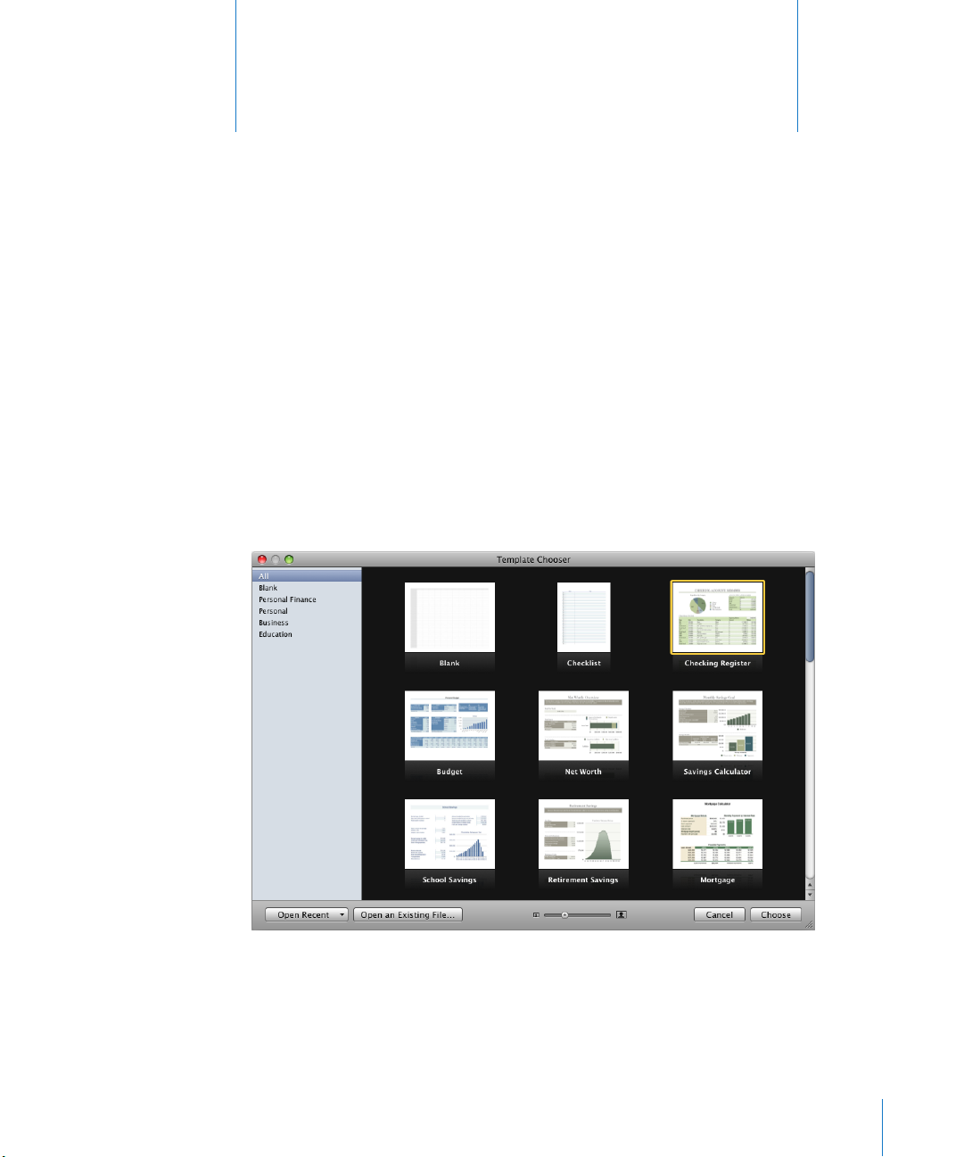
Spreadsheet Templates

When you rst open the Numbers application (by clicking its icon in the Dock or

double-clicking its icon in the Finder), the Template Chooser window presents a variety of spreadsheet templates from which to choose.

Templates contain predened sheets, tables, formulas, and other elements that help

you get started.

Here are ways to use the Template Chooser window:

To view thumbnails of all the templates, click All in the list of template categories on m the left side of the Template Chooser window.

To view templates by category, click Blank, Personal Finance, or another category.

To increase or decrease the size of the thumbnails, drag the slider at the bottom of the m window.

To create a spreadsheet using a specic template, click the template and then click m

Choose.

If you want to start from a plain spreadsheet, without preformatting, pick the Blank template.

See “Creating a New Spreadsheet” on page 28, “ Importing a Document from Another Application” on page 29, and “Using CSV or OFX Files in a Spreadsheet” on page 30 to learn how to create a Numbers spreadsheet.

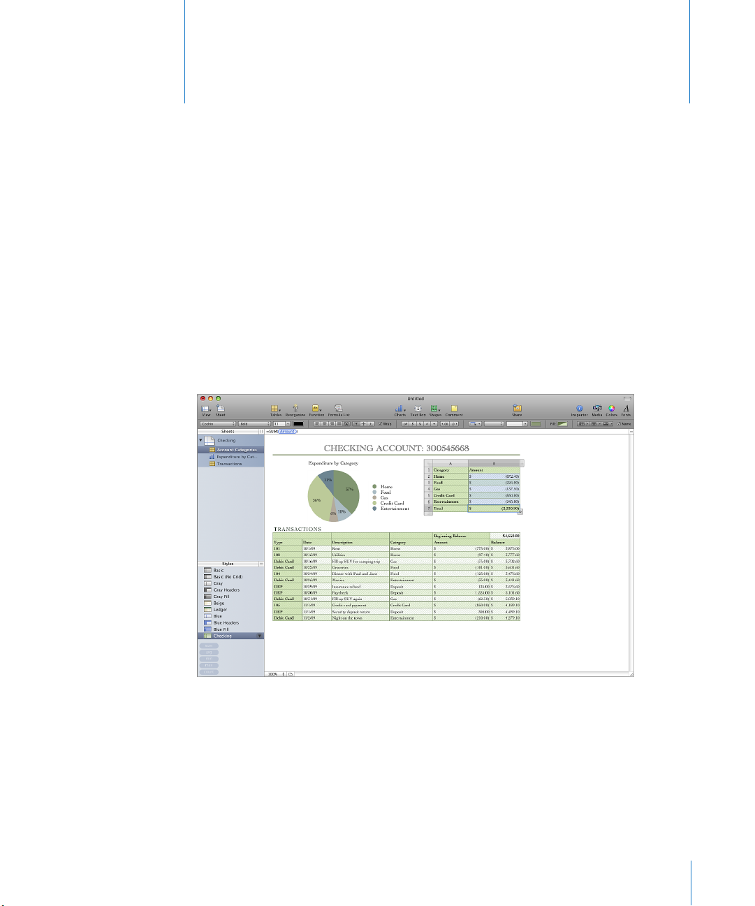
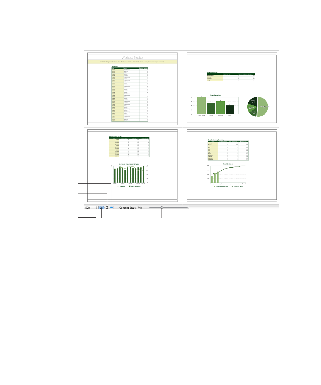
The Numbers Window

The Numbers window has elements that help you develop and organize your spreadsheet.

Sheets pane: This pane, in the upper left, lists the tables and charts on each sheet in the spreadsheet. Sheets organize your information into groups of related items (for example, data for 2008 and data for 2009). Drag the Sheets resize control, located at the top right of the Sheets pane, left or right to make the pane wider or narrower.

14 Chapter 1 Numbers Tools and Techniques

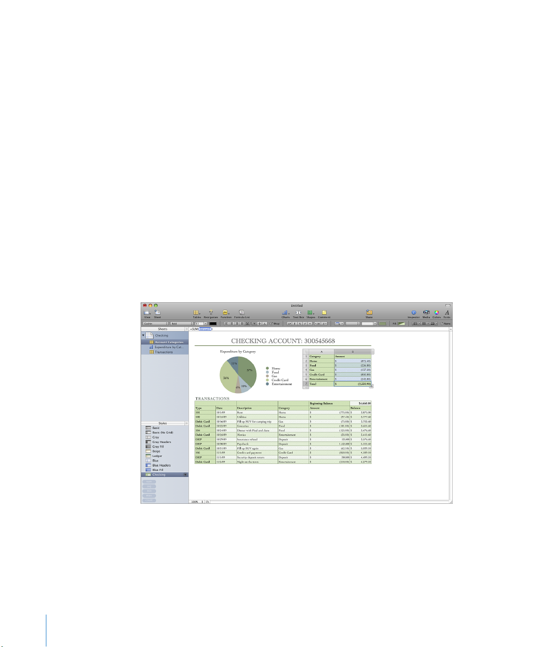
Toolbar: Located at the top of the window, the toolbar gives you one-click access

to commonly used tools. Use it to quickly add a sheet, table, text box, media le, and

other objects.

Format bar: Below the toolbar, the format bar provides convenient access to tools for editing a selected object.

Formula bar: Below the format bar, the formula bar lets you create and edit formulas or other content in a selected table cell.

Sheet canvas: The main part of the window, the sheet canvas shows objects on a selected sheet. You can drag tables, charts, and other objects on the sheet canvas to rearrange them.

Styles pane: Below the Sheets pane, the Styles pane lists table styles predesigned for the template you’re using. Select a table, and click a table style to instantly change the table’s appearance. Drag the Styles resize control, located at the top right of the Styles pane, up or down to enlarge or shrink the pane.

Instant calculation results: Below the Styles pane is an area that displays the results of calculations for values in selected table cells.

To learn about Go to

Viewing a spreadsheet “Zooming In or Out” on page 16

“The Sheets Pane” on page 16

“Print View” on page 17

“Freezing Table Header Rows and Header Columns” on page 60

Tools for managing spreadsheets “The Toolbar” on page 17

“The Format Bar” on page 18

“The Inspector Window” on page 19

“The Warnings Window” on page 26

Tools for working with formulas in table cells “Formula Tools” on page 20

Tools that enhance the appearance of a spreadsheet

Keyboard shortcuts “Keyboard Shortcuts and Shortcut Menus” on

“The Styles Pane” on page 21

“The Media Browser” on page 23

“The Colors Window” on page 24

“The Fonts Window” on page 25

page 27

Chapter 1 Numbers Tools and Techniques 15

Zooming In or Out

Click to show or hide a

sheet’s tables and charts

in the Sheets pane.

Drag left or right to resize the Sheets pane.

Click a table or chart in the list to select it and show it on the sheet canvas.

You can enlarge (zoom in) or reduce (zoom out) your view of a sheet.

Here are ways to zoom in or out on a sheet:

Choose View > Zoom > Zoom In or View > Zoom > Zoom Out. m

To return to 100%, choose View > Zoom > Actual Size.

Choose a magnication level from the pop-up menu at the bottom left of the canvas. m

When you view a sheet in Print View, decrease the zoom level to view more pages in the window at one time.

The Sheets Pane

The Sheets pane is located along the top left side of the Numbers window. It lets you quickly view and navigate to tables and charts in a sheet.

See “Using Sheets to Organize a Spreadsheet” on page 36 for more information.

16 Chapter 1 Numbers Tools and Techniques

Print View

Click to show or hide Print View.

Slide to shrink or enlarge all the sheet’s objects.

Footer area

Header area

Click to choose a page

zoom level that lets you

see more or fewer pages.

Click to view pages in

portrait (vertical)

orientation.

Click to view pages in

landscape (horizontal)

orientation.

When you want to print a sheet or make a PDF of it, you can use Print View to visualize the layout of a sheet’s objects on individual pages.

Chapter 1 Numbers Tools and Techniques 17

See “Dividing a Sheet into Pages” on page 39 to learn more about Print View.

The Toolbar

The Numbers toolbar gives you one-click access to many of the actions you perform as you work in Numbers. As you discover which actions you perform most often, you can add, remove, and rearrange toolbar buttons to suit your working style. You can also hide the toolbar by choosing View > Hide Toolbar; to show it again, choose View > Show Toolbar.

To see a description of what a button does, hold your pointer over it.

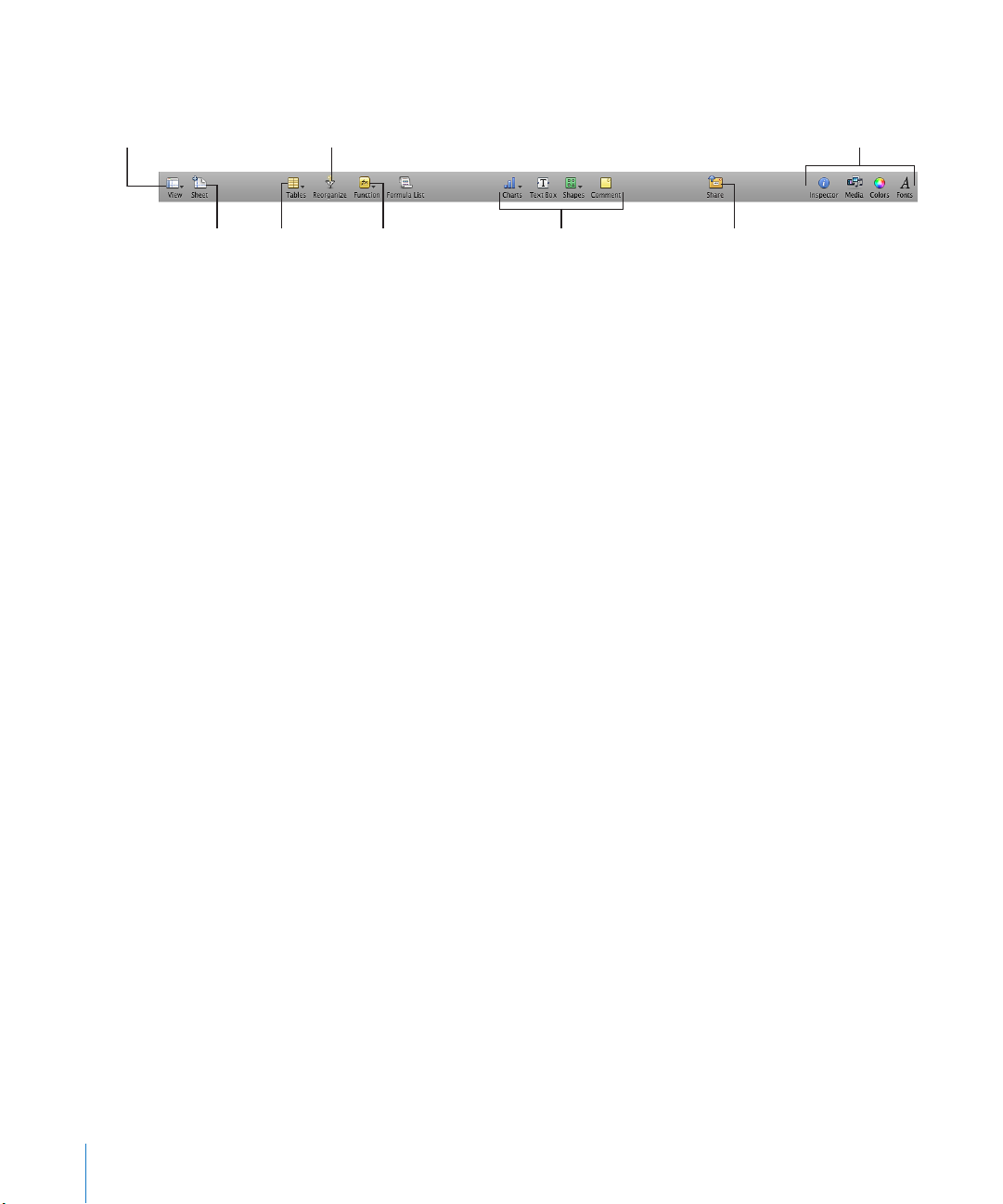
The default set of toolbar buttons is shown below.

Open the inspector window,

Media Browser, Colors

window, or Fonts window.

Publish the spreadsheet on the web.

Add a chart, text box, shape, or comment.

Add a table.

Add a formula or function.

Sort, filter, and categorize rows.

Add a sheet.

Show or hide Print View, comments, and more.

To customize the toolbar:

1 Choose View > Customize Toolbar. The Customize Toolbar sheet appears.

2 Make changes to the toolbar as desired.

To add an item to the toolbar, drag its icon to the toolbar. If you frequently Â

recongure the toolbar, you can add the Customize button to it.

To remove an item from the toolbar, drag it out of the toolbar. Â

To restore the default set of toolbar buttons, drag the default set to the toolbar. Â

To make the toolbar icons smaller, select Use Small Size. Â

To display only icons or only text, choose an option from the Show pop-up menu. Â

To rearrange items in the toolbar, drag them. Â

3 Click Done.

You can also customize the toolbar by using these shortcuts:

To remove an item from the toolbar, press the Command key while dragging the Â item out of the toolbar.

You can also press the Control key while you click the item, and then choose Remove Item from the shortcut menu.

To move an item, press the Command key while dragging the item around in the Â toolbar.

The Format Bar

Use the format bar, displayed below the toolbar, to quickly change the appearance of tables, charts, text, and other elements in your spreadsheet.

The controls in the format bar vary with the object selected. To see a description of what a format bar control does, hold the pointer over it.

18 Chapter 1 Numbers Tools and Techniques

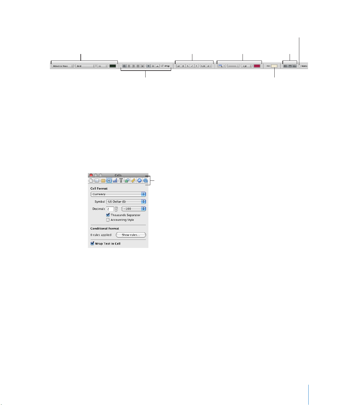
Here’s what the format bar looks like when a table or table cell is selected:

Arrange text in table cells.

Format cell borders.

Add background

color to a cell.

Format cell values.

Manage headers

and footers.

Show or hide a table’s name.

Format text in

table cells.

The buttons at the top of the inspector window open the ten inspectors: Document, Sheet, Table, Cells, Chart, Text, Graphic, Metrics, Hyperlink, and QuickTime.

To show and hide the format bar:

Choose View > Show Format Bar or View > Hide Format Bar. m

The Inspector Window

Most elements of your spreadsheet can be formatted using the Numbers inspectors.

Each inspector focuses on a dierent aspect of formatting. For example, the Cells

inspector lets you format cells and cell values. Hold your pointer over buttons and other controls in the inspector panes to see a description of what the controls do.

Opening multiple inspector windows can make it easier to work on your spreadsheet. For example, you can open both the Graphic inspector and the Cells inspector to have access to all the image- and cell-formatting options.

After an inspector window is open, click any of the buttons at the top to display a dierent inspector. Clicking the second button from the left, for example, displays the Sheet inspector.

Here are ways to open an inspector window:

Click Inspector in the toolbar. m

Chapter 1 Numbers Tools and Techniques 19

Choose View > Show Inspector. m

To open another Inspector window, choose View > New Inspector. m

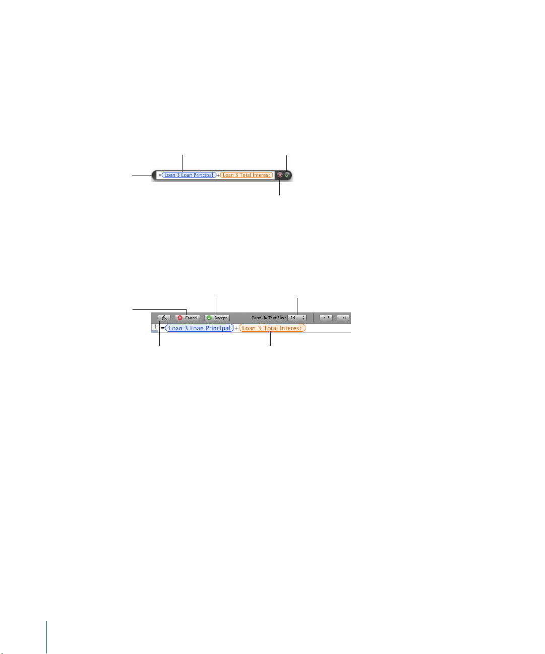
Formula Tools

Cancel button

Discard changes.

Accept button

Save changes.

Text field

View or edit a formula.

Formula Editor

Move by grabbing

here and dragging.

Open the Function Browser.

Cancel button

Discard changes.

Accept button

Save changes.

Change the formula viewing size.

Text field

View or edit a formula.

You add a formula to a table cell when you want to display a value in the cell that’s derived using a calculation. Numbers has several tools for working with formulas in table cells:

The Â Formula Editor lets you create and modify formulas. Open the Formula Editor by selecting a table cell and typing the equal sign (=). You can also open it by choosing Formula Editor from the Function pop-up menu in the toolbar.

Learn more about this editor in “Adding and Editing Formulas Using the Formula Editor” on page 11 9 .

The Â formula bar, always visible below the format bar, can also be used to create and modify a formula in a selected table cell.

Instructions for adding and editing formulas using this tool are in “Adding and Editing Formulas Using the Formula Bar” on page 12 0 .

20 Chapter 1 Numbers Tools and Techniques

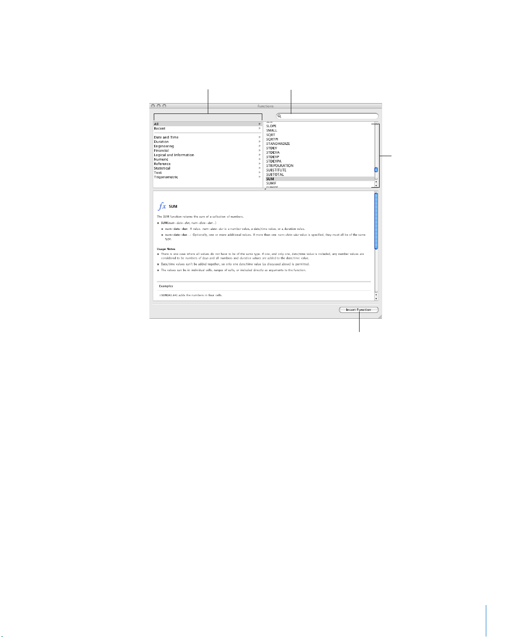
Using the Â Function Browser is the fastest way to add a function. A function is

Select a function to view information about it.

Search for a function.

Insert the selected function.

Select a category to view functions in that category.

a predened formula that has a name (such as SUM and AVERAGE).

To open the Function Browser, choose Show Function Browser from the Function pop-up menu in the toolbar.

“Adding Functions to Formulas” on page 121 explains how to use the Function Browser. To learn about all the iWork functions, and to review numerous examples that illustrate how to use them, choose Help > “iWork Formulas and Functions Help” or Help > “iWork Formulas and Functions User Guide.”

The Styles Pane

The Styles pane lets you quickly apply predened formatting to tables in a spreadsheet. Table styles dene such attributes as color, text size, and cell

border formatting of table cells.

Chapter 1 Numbers Tools and Techniques 21

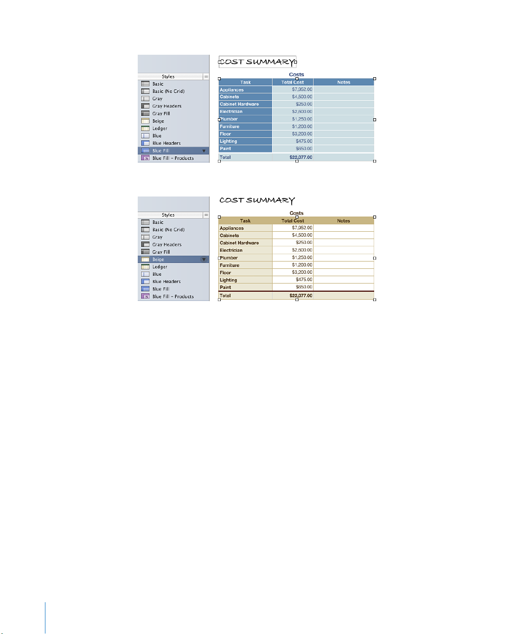
To apply a table style, simply select the table and click a style in the Styles pane.

Switching from one table style to another takes only one click.

See “Using Table Styles” on page 111 for details.

22 Chapter 1 Numbers Tools and Techniques

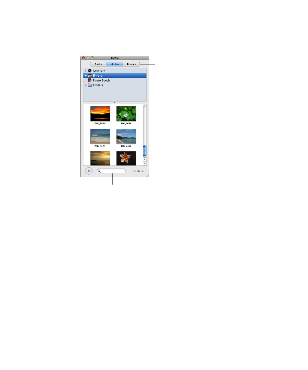
The Media Browser

Second, choose a source.

First, click a button to go to your media files.

Third, drag an item to the document or to an image well in one of the inspectors.

Search for a file by typing its name here.

The Media Browser provides access to all the media les in your iPhoto library, your

iTunes library, and your Movies folder. You can drag an item from the Media Browser to your spreadsheet or to an image well in an inspector.

If you don’t use iPhoto or Aperture to store your photos, or iTunes to store your music, or if you don’t keep your movies in the Movies folder, you can add other folders to the Media Browser so that you can access their multimedia contents in the same way.

Here are ways to open the Media Browser:

Click Media in the toolbar. m

Choose View > Show Media Browser. m

Here are ways to add other folders to the Media Browser:

To add a folder containing audio les, click Audio in the Media Browser, and then drag m

the folder you want from the Finder to the Media Browser.

To add a folder containing photos, click Photos in the Media Browser, and then drag m the folder you want from the Finder to the Media Browser.

To add a folder containing movies, click Movies in the Media Browser, and then drag m the folder you want from the Finder to the Media Browser.

Chapter 1 Numbers Tools and Techniques 23

To learn how to Go to

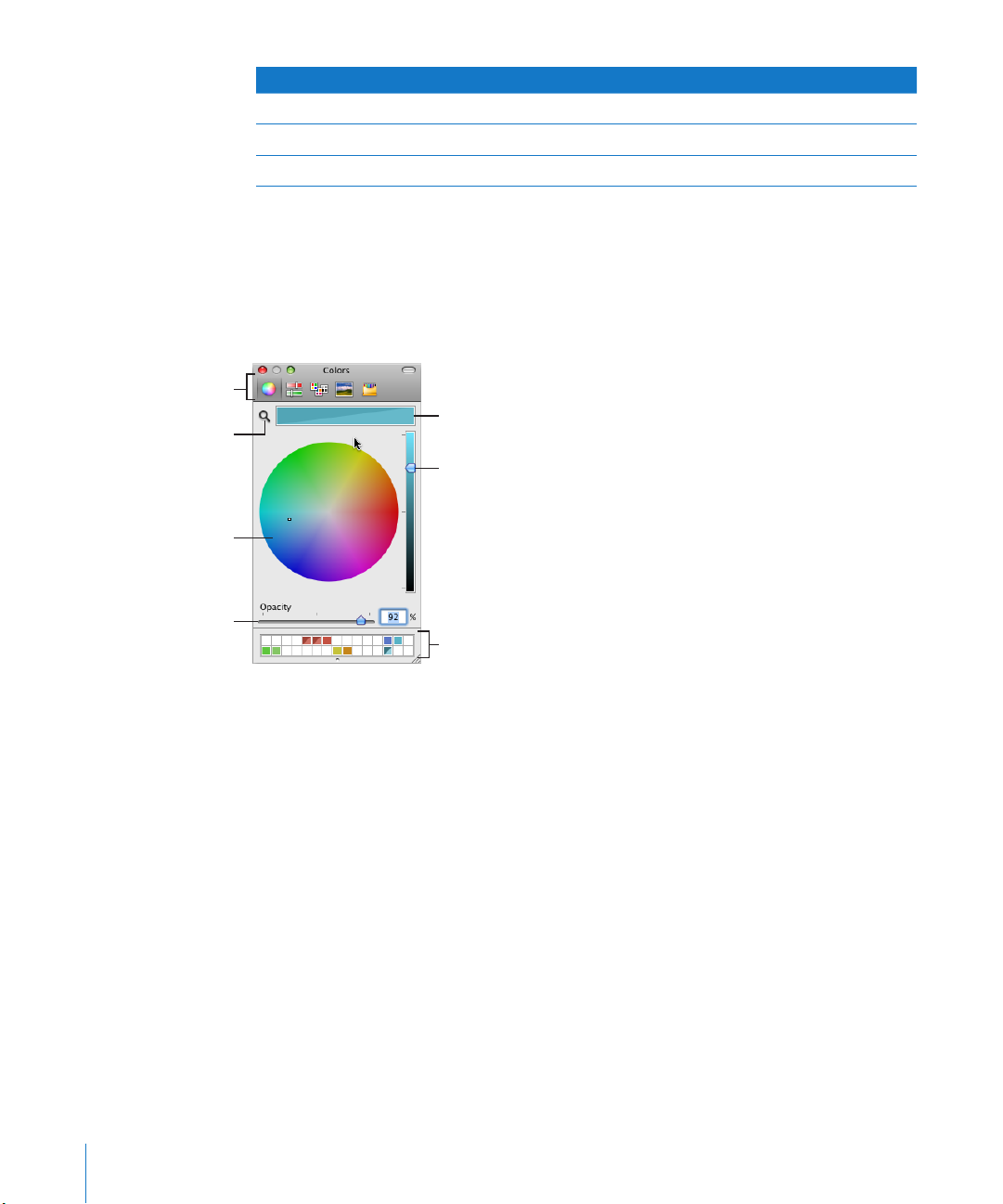
The color selected in the color wheel appears in this box. (The two colors in this box indicate the opacity is set to less than 100%.)

Use the slider to set lighter or darker hues in the color wheel.

Click to select a color in

the color wheel.

Drag colors from the color box to store them in the color palette.

Click the search icon,

and then click any

item on the screen to

match its color.

Click a button to view

different color models.

Drag the Opacity slider

to the left to make the

color more transparent.

Import an image “Working with Images” on page 191

Add a sound le “Adding a Sound File” on page 206

Add a movie le “Adding a Movie File” on page 207

The Colors Window

You use the Colors window to apply color to text, table cells, cell borders, and other objects. While you can also use the format bar to apply colors, the Colors window

oers advanced color management options.

You can use the color wheel in the Colors window to select colors. The color you select appears in the box at the top of the Colors window. You can save that color for future use by placing it in the color palette.

To apply the colors you select in the Colors window to an object, select the object and then place the color in the appropriate color well in an inspector. You can click a color well in one of the inspectors and then click a color in the color well. Or you can drag a color from the color palette or color box to a color well in an inspector.

Here are ways to open the Colors window:

Click Colors in the toolbar. m

1 Click anywhere in the color wheel.

24 Chapter 1 Numbers Tools and Techniques

Click a color well in one of the inspectors. m

To select a color after opening the Colors window:

The selected color is displayed in the color box at the top of the Colors window.

2 To make the color lighter or darker, drag the slider on the right side of the Colors

Create interesting

text effects using

these buttons.

The Action menu

Choose a typeface to apply to selected text.

Find fonts by typing a font

name in the search field.

Choose a font size to apply to selected text.

Apply a shadow to selected text. Modify the shadow using the opacity, blur, offset, and angle controls.

Preview the selected

typeface (you might need to

choose Show Preview from

the Action menu).

window.

3 To make the color more transparent, drag the Opacity slider to the left or enter

a percentage value in the Opacity eld.

4 To use the color palette, open it by dragging the handle at the bottom of the Colors

window.

Save a color in the palette by dragging a color from the color box to the color palette. To remove a color from the palette, drag a blank square to the color you want to remove.

5 To match the color of another item on the screen, click the search icon to the left of

the color box in the Colors window.

Click the item on the screen whose color you want to match. The color appears in the color box. Select the item you want to color in the spreadsheet, and then drag the color from the color box to the item.

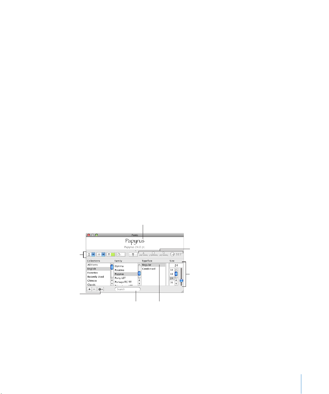
The Fonts Window

Use the Fonts window to select fonts, font sizes, and other font formatting features, including text shadows and strikethrough. You can also use the Fonts window to

organize your favorite and commonly used fonts so that they are easy to nd when

you need them.

To open the Fonts window:

Click Fonts in the toolbar. m

Here are ways to change the font of selected text:

In the Search eld, type the name of the font you want to use, and then select its m

name in the Family list.

Chapter 1 Numbers Tools and Techniques 25

Select a typeface (for example, Italic or Bold) from the Typeface list. m

In the Size column, type or select the font size you want. m

Here are ways to use the controls at the top of the Fonts window:

Rest your pointer over any control along the top of the window to view a help tag

describing what each control does. If you don’t see the controls, choose Show Eects

from the Action pop-up menu (looks like a gear) in the lower-left corner of the window.

To underline text, choose an underline style (such as single or double) from the Text m Underline pop-up menu.

To apply a strikethrough style (such as single or double), choose a style from the Text m Strikethrough pop-up menu.

To apply color to text, click the Text Color button to open the Colors window. See “ m The Colors Window” on page 24 for details.

To apply color behind a paragraph, click the Document Color button to open the m Colors window.

To apply a shadow, click the Text Shadow button. Use the Shadow Opacity, Shadow m

Blur, Shadow Oset, and Shadow Angle controls to format the shadow.

To organize fonts:

1 Click the Add Collection (+) button to create and name a new collection.

2 Select some text and format it with the font family, typeface, and size that you want.

3 Drag the font name from the Family list to the collection where you want to le it.

To set up the Fonts window for frequent use:

Leave the Fonts window open as you work. Resize the window using the control in the m

bottom-right corner of the window so that only the font families and typefaces in your selected font collection are visible.

The Warnings Window

When you import a document into Numbers, or export a Numbers spreadsheet to another format, some elements might not transfer as expected. The Document Warnings window lists any problems encountered.

If there are problems, you’ll see a message enabling you to review the warnings. If you choose not to review them, you can see the Warnings window at any time by choosing View > Show Document Warnings.

If you see a warning about a missing font, you can select the warning and click Replace Font to choose a replacement font.

26 Chapter 1 Numbers Tools and Techniques

You can copy one or more warnings by selecting them in the Document Warnings window and choosing Edit > Copy. You can then paste the copied text into an email

message, text le, or some other window.

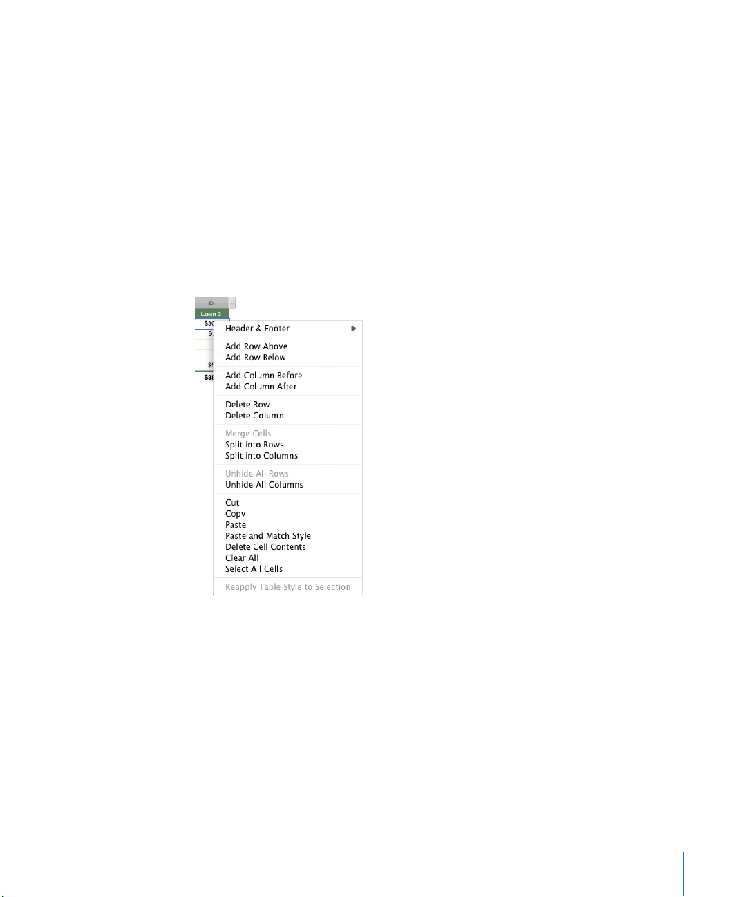
Keyboard Shortcuts and Shortcut Menus

You can use the keyboard to perform many Numbers tasks. To see a comprehensive list of keyboard shortcuts, open Numbers and choose Help > Keyboard Shortcuts.

Many objects also have shortcut menus with commands you can use on the object. Shortcut menus are especially useful for working with tables and charts.

To open a shortcut menu:

Press the Control key while you click an object. m

Chapter 1 Numbers Tools and Techniques 27

Creating, Saving, and Organizing a Numbers Spreadsheet

This chapter describes how to manage Numbers spreadsheets.

You can create a Numbers spreadsheet by opening Numbers and choosing a template. You can also import a document created in another application, such as Microsoft Excel or AppleWorks 6, or create a spreadsheet using a CSV

(comma-separated value) le.

This chapter explains how to create new Numbers spreadsheets, as well as how to open existing spreadsheets and save spreadsheets.

This chapter also provides instructions for organizing spreadsheets into sheets and for organizing them into pages when you print them or create PDFs.

Creating a New Spreadsheet

To create a new Numbers spreadsheet, you pick the template that provides appropriate formatting and content characteristics.

Start with the Blank template to build your spreadsheet from scratch. Or select one of the many other templates to get a head start creating a budget, planning a party, and

more using predened tables, charts, and sample data.

To create a new spreadsheet:

1 Open Numbers by clicking its icon in the Dock or by double-clicking its icon

in the Finder.

If Numbers is open, choose File > “New from Template Chooser.”

2 In the Template Chooser window, select a template category in the left column

to display related templates, and then select the template that best matches the spreadsheet you want to create. If you want to begin in a spreadsheet without any

predened content, select Blank.

You can skim the contents of a template by moving the pointer left and right over its icon. To change the size of the template icons, drag the slider at the bottom of the window.

3 After selecting a template, click Choose. A new spreadsheet opens on your screen.

You can set Numbers to automatically open a particular template every time you open Numbers or create a new spreadsheet. Choose Numbers > Preferences, click General, select “For New Documents: Use template:”, and then click Choose. Select a template name, and then click Choose.

Each time the Template Chooser opens, the previously selected template category and template are selected.

Importing a Document from Another Application

You can create a new Numbers spreadsheet by importing a document created in

Microsoft Excel or AppleWorks 6. Numbers can also import les in comma-separated

value (CSV) format, tab-delimited format, and Open Financial Exchange (OFX) format.

From AppleWorks, you can import spreadsheets only.

Chapter 2 Creating, Saving, and Organizing a Numbers Spreadsheet 29

Here are ways to import a document:

Drag the document to the Numbers application icon. A new Numbers spreadsheet m opens, and the contents of the imported document are displayed.

In Numbers, choose File > Open, select the document, and then click Open. m

You can import Address Book data to quickly create tables that contain names, phone m numbers, addresses, and other information for your contacts. See “Using Address Book Fields” on page 228 for instructions.

If you want to import CSV or OFX data, see “ m Using CSV or OFX Files in a Spreadsheet” on page 30.

If you can’t import a document, try opening the document in another application and saving it in a format Numbers can read, or copy and paste the contents into an existing Numbers spreadsheet.

You can also export Numbers spreadsheets to Microsoft Excel, PDF, and CSV les. See

“Exporting a Spreadsheet to Other Document Formats” on page 234 for details.

Using CSV or OFX Files in a Spreadsheet

To add CSV or OFX data to an open spreadsheet:

1 Select a sheet.

2 Do one of the following:

To create one or more new tables, drag a CSV or OFX le from the Finder onto the Â

sheet’s canvas.

To add CSV or OFX data to an empty table, drag the CSV or OFX le onto the table. Â

The data is added; additional columns are created if necessary.

To add CSV or OFX data to a table that contains data, drag the CSV or OFX le onto Â

the table.

If the columns don’t match, choose an option from the sheet that appears. You can cancel the import, add columns to the table, ignore extra columns, or create a new table from the CSV or OFX data.

Opening an Existing Spreadsheet

You can open an iWork ’08 or iWork ’09 spreadsheet. To take advantage of new features, save iWork ’08 spreadsheets in iWork ’09 format. To let iWork ’08 users access your spreadsheet, save it in iWork ’08 format.

When you open an iWork ’09 spreadsheet that’s password-protected, you need to type

the password in the Password eld before you can view the spreadsheet contents.

30 Chapter 2 Creating, Saving, and Organizing a Numbers Spreadsheet

Here are ways to open an existing spreadsheet:

To open a spreadsheet from the Template Chooser, click “Open an Existing File” in the m Template Chooser window, select the document, and then click Open.

To open a spreadsheet you’ve worked with recently, choose it from the Open Recent pop-up menu at the bottom left of the Template Chooser window.

To open a spreadsheet when you’re working in one, choose File > Open, select the m spreadsheet, and then click Open.

To open a spreadsheet you’ve worked with recently, choose File > Open Recent and choose the spreadsheet from the submenu.

To open a Numbers spreadsheet from the Finder, double-click the spreadsheet icon or m drag it to the Numbers application icon.

If you see a message that a font or le is missing when you open a spreadsheet, you

can still use the spreadsheet. Numbers lets you choose fonts to substitute for missing fonts. Or you can add missing fonts by quitting Numbers and adding the fonts to your Fonts folder (for more information, see Mac Help). To make missing movies or sound

les reappear, add them to the spreadsheet again.

Password-Protecting a Spreadsheet

When you want to restrict access to a Numbers document, you can assign it a password. Passwords can consist of almost any combination of numerals and capital or lowercase letters and several of the special keyboard characters. Passwords with combinations of letters, numbers, and other characters are generally considered more secure.

When you save a spreadsheet in iWork ’08 or Excel format, you can’t use password protection, but when you export a spreadsheet as a PDF you can assign a password to it.

Here are ways to manage password-protection in a Numbers spreadsheet:

To use a password-protected spreadsheet, open the spreadsheet, type the password m when prompted, optionally select “Remember this password in my keychain,” and then click OK.

If you incorrectly type the password twice, any hint dened when the password was

created is displayed.

To add a password to the spreadsheet, open the Document inspector and select m “Require password to open” in the Document pane. Type the password you want to use in the elds provided, and then click Set Password. A lock icon appears next to the document title to indicate that your document is password protected.

Chapter 2 Creating, Saving, and Organizing a Numbers Spreadsheet 31

If you want help to create an unusual or strong password, click the button with the

key-shaped icon next to the Password eld to open the Password Assistant and use it

to help you create a password. You can select a type of password in the pop-up menu, depending on which password characteristics are most important to you.

A password appears in the Suggestion eld; its strength (“stronger” passwords are more dicult to break) is indicated by the length and green color of the Quality bar. If you like the suggested password, copy it and paste it into the Password eld.

If you don’t like the suggested password, you can choose a dierent password from the Suggestion eld pop-up menu, increase the password length by dragging the

slider, or type your own.

To remove a password from a spreadsheet, open your password-protected document, m and then deselect “Require password to open” in the Document inspector’s Document pane. Type the document password to disable password protection and click OK.

To change a password, open the Document inspector, click Change Password, enter m your information, and then click Change Password.

To add a password for a PDF of your spreadsheet, follow the instructions in “ m Exporting a Spreadsheet in PDF Format” on page 234.

Saving Spreadsheets

It’s a good idea to save your spreadsheet often as you work. After you save it for the

rst time, you can press Command-S to resave it using the same settings.

When you save a Numbers spreadsheet, fonts are not included as part of the spreadsheet. If you transfer a Numbers spreadsheet to another computer, make sure the fonts used in the spreadsheet have been installed in the Fonts folder of that computer.

To save a spreadsheet for the rst time:

1 Choose File > Save, or press Command-S.

2 In the Save As eld, type a name for the spreadsheet.

3 Choose where you want to save the spreadsheet.

If the directory in which you want to save the spreadsheet isn’t visible in the Where

pop-up menu, click the disclosure triangle to the right of the Save As eld and navigate to a dierent location.

4 If you want the spreadsheet to display a Quick Look in the Finder in Mac OS X version

10.5 or later, select “Include preview in document.”

If you always want to include a preview in your spreadsheets, choose Numbers > Preferences, click General, and select “Include preview in document by default.”

32 Chapter 2 Creating, Saving, and Organizing a Numbers Spreadsheet

5 If you want to save the spreadsheet as an iWork ’08 or Excel spreadsheet, select “Save

copy as” and choose iWork ’08 or Excel Document from the pop-up menu.

6 If you or someone else will open the spreadsheet on another computer, click

Advanced Options and set up options that determine what’s copied into your spreadsheet.

Copy audio and movies into document: If you use movies or sound les in your spreadsheet, selecting this checkbox saves the movie or sound les with the spreadsheet so the les play if the spreadsheet is opened on another computer. You can deselect this checkbox so that the le size is smaller, but the media les won’t

play on other computers. See “Reducing Image File Sizes” on page 195 and “Reducing the Size of Media Files” on page 209 to learn other techniques for reducing le size.

Copy template images into document: If you don’t select this option and you open the spreadsheet on a computer that doesn’t have Numbers installed, the spreadsheet

might look dierent.

7 Click Save.

In general, you can save Numbers spreadsheets only to computers and servers that use Mac OS X. Numbers is not compatible with Mac OS 9 computers and Windows servers running Services for Macintosh. If you must save to a Windows computer, try using AFP server software available for Windows to do so.

To learn how to Go to

Share your spreadsheets with others “Printing a Spreadsheet” on page 233

“Sending Your Numbers Spreadsheet to iWork. com public beta” on page 236

“Exporting a Spreadsheet to Other Document Formats” on page 234

“Sending a Spreadsheet Using Email” on page 239

“Sending a Spreadsheet to iWeb” on page 239

Undo changes made since opening a spreadsheet or last saving it

Save dierent versions of a spreadsheet “Automatically Saving a Backup Version” on

Save terms that Spotlight can use to locate a spreadsheet

Close a spreadsheet without quitting “Closing a Spreadsheet Without Quitting

“Undoing Changes” on page 34

page 34

“Saving a Copy of a Spreadsheet” on page 35

“Saving a Spreadsheet as a Template” on page 34

“Saving Spotlight Search Terms for a Spreadsheet” on page 35

Numbers” on page 35

Chapter 2 Creating, Saving, and Organizing a Numbers Spreadsheet 33

Undoing Changes

If you don’t want to save changes you made to your spreadsheet since opening it or last saving it, you can undo them.

Here are ways to undo changes:

To undo your most recent change, choose Edit > Undo. m

To undo multiple changes, choose Edit > Undo multiple times. You can undo m any changes you made since opening the spreadsheet or reverting to the last saved version.

To restore changes you’ve undone using Edit > Undo, choose Edit > Redo one or m more times.

To undo all changes you made since the last time you saved your spreadsheet, choose m File > “Revert to Saved” and then click Revert.

Automatically Saving a Backup Version

Each time you save a spreadsheet, you can save a copy without the changes you made since last saving it. That way, if you change your mind about edits you’ve made, you can go back to (revert to) the backup version of the spreadsheet.

Here are ways to create and use a backup version:

To automatically save a backup version of a spreadsheet, choose Numbers > m Preferences, click General, and then select “Back up previous version when saving.”

The next time you save your spreadsheet, a backup version is created in the same

location, with “Backup of” preceding the lename. Only one version—the last saved version—is backed up. Every time you save the spreadsheet, the old backup le is replaced with the new backup le.

To revert to the last saved version after making unsaved changes, choose File > “Revert m to Saved.” The changes in your open spreadsheet are undone.

Saving a Spreadsheet as a Template

To use a spreadsheet you’ve created as a starting point for future documents, you can save the spreadsheet as a template. When you save a spreadsheet as a template, it appears in the Template Chooser.

To save a spreadsheet as a template:

Choose File > “Save as Template.” m

See “Designing a Template” on page 241 for additional details.

34 Chapter 2 Creating, Saving, and Organizing a Numbers Spreadsheet

Saving Spotlight Search Terms for a Spreadsheet

You can store such information as author name and keywords in Numbers spreadsheets, and then use Spotlight to locate spreadsheets containing that information.

To store Spotlight terms:

1 Click Inspector in the toolbar, and then click the Document inspector button.

2 In the Spotlight elds, enter or change information.

To search for spreadsheets containing Spotlight information, click the Spotlight icon at the top right of the menu bar, and then type what you want to search for.

Saving a Copy of a Spreadsheet

If you want to make a copy of your spreadsheet (for example, to create a backup copy

or multiple versions), you can save it using a dierent name or location. (You can also

automate saving a backup version, as “Automatically Saving a Backup Version” on page 34 describes.)

To save a copy of a spreadsheet:

Choose File > Save As and specify a name and location. m

The spreadsheet with the new name remains open. To work with the previous version, choose File > Open Recent and choose the previous version from the submenu.

Closing a Spreadsheet Without Quitting Numbers

When you have nished working with a spreadsheet, you can close it without quitting

Numbers.

Chapter 2 Creating, Saving, and Organizing a Numbers Spreadsheet 35

Here are ways to close the active spreadsheet and keep the application open:

Click to show or hide a

sheet’s tables and charts

in the Sheets pane.

Drag left or right to resize the Sheets pane.

Click a table or chart in the list to select it and show it on the sheet canvas.

To close the active spreadsheet, choose File > Close or click the close button in the m upper-left corner of the Numbers window.

To close all open spreadsheets, press the Option key and choose File > Close All or m click the active spreadsheet’s close button.

If you’ve made changes since you last saved the spreadsheet, Numbers prompts you to save.

Using Sheets to Organize a Spreadsheet

Like chapters in a book, sheets let you divide information into manageable groups. For

example, you might want to place charts in the same sheet as the tables whose data they display. Or you may want to place all the tables on one sheet and all the charts on another sheet. You might want to use one sheet for keeping track of business contacts and other sheets for friends and relatives.

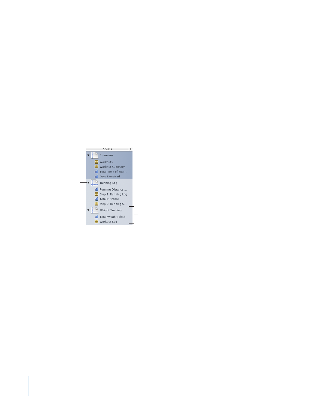
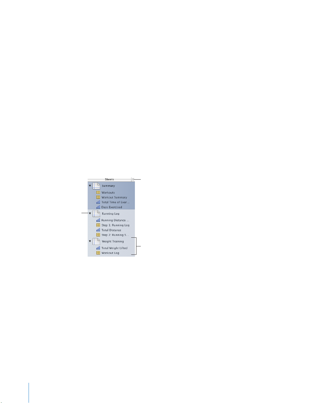
The sheets in a spreadsheet and the tables and charts on each sheet are represented in the Sheets pane, located along the left edge of the window.

Only tables and charts are listed for any sheet, even if you have text, images, and other objects in your spreadsheet.

The order of a sheet’s tables and charts in the Sheets pane may not match their order in the spreadsheet, as “Reorganizing Sheets and Their Contents” on page 37 describes.

Here are ways to see a sheet’s objects:

To show or hide all a sheet’s tables and charts in the Sheets pane, click the disclosure m triangle to the left of the sheet in the pane.

To display the contents of a sheet, click the sheet in the Sheets pane. m

When you’re working on a table or chart in a spreadsheet, the table or chart is

36 Chapter 2 Creating, Saving, and Organizing a Numbers Spreadsheet

highlighted in the Sheets pane.

To learn how to Go to

Create and remove sheets “Adding and Deleting Sheets” on page 37

Move sheets around, reorder their tables and charts, and move tables and charts among sheets

Name a sheet “Changing Sheet Names” on page 38

“Reorganizing Sheets and Their Contents” on page 37

Adding and Deleting Sheets

Here are ways to create and remove sheets:

To add a new sheet, click the Sheet button in the toolbar. You can also choose m Insert > Sheet.

A new sheet containing a predened table is added at the bottom of the Sheets pane.

You can move the sheet by dragging it to a new location in the Sheets pane.

When you add a sheet, Numbers assigns it a default name, but you can change the name, as “Changing Sheet Names” on page 38 describes.

To copy a sheet, do any of the following: m

Option-drag the sheet you want to copy to the desired location in the Sheets pane. Â

Make a copy using Edit > Duplicate, which inserts the copy immediately after the Â selected sheet.

In the Sheets pane, select a sheet to copy, choose Edit > Copy, select the sheet after Â which you want the copy located, and choose Edit > Paste.

To delete a sheet and its contents, select it in the Sheets pane and press the m Delete key.

Reorganizing Sheets and Their Contents

In the Sheets pane, you can move sheets around and reorder their tables and charts. You can also move tables and charts from one sheet to another.

Reordering tables and charts in the Sheets pane doesn’t aect their location on the

sheet canvas. In the Sheets pane, for example, you may want to place charts next to the tables they’re derived from, or list tables in the order in which you want to work

on them. But on the sheet canvas, you may want to present these objects in a dierent

order (for example, when you lay out your spreadsheet for printing).

Here are ways to reorganize sheets in the Sheets pane:

To move a sheet, select it and drag it to a new location in the pane. Sheets shift as m you drag.

You can also select multiple sheets and move them as a group.

Chapter 2 Creating, Saving, and Organizing a Numbers Spreadsheet 37

To copy (or cut) and paste sheets, select the sheets, choose Edit > Cut or Edit > Copy, m select the sheet after which you want to place the sheets you’re moving, and choose Edit > Paste.

To move one or more tables and charts associated with a sheet, select them and drag m

them to a new location in the same sheet or to a dierent sheet.

You can also use cut/paste or copy/paste actions to move tables and charts in the pane.

To move an object within a sheet in the spreadsheet, select it and drag it to a dierent location, or use cut/paste or copy/paste actions. To place objects on specic pages for

printing or creating a PDF, follow the instructions in “Dividing a Sheet into Pages” on page 39.

Changing Sheet Names

A name distinguishes each sheet in the Sheets pane. The sheet name is assigned by default when you add a sheet, but you can change it to a more descriptive name.

Here are ways to change a sheet’s name:

In the Sheets pane, double-click the name and edit it. m

Select the sheet in the Sheets pane or an object on the sheet, and in the Sheet m

inspector, edit the name in the Name eld.

You can also change the names of a sheet’s tables and charts. See “Naming Tables” on page 49 and “Placing and Formatting a Chart’s Title and Legend” on page 141 for instructions.

38 Chapter 2 Creating, Saving, and Organizing a Numbers Spreadsheet

Dividing a Sheet into Pages

Click to show or hide Print View.

Slide to shrink or enlarge all the sheet’s objects.

Footer area

Header area

Click to choose a page

zoom level that lets you

see more or fewer pages.

Click to view pages in

portrait (vertical)

orientation.

Click to view pages in

landscape (horizontal)

orientation.

Using Print View, you can view a sheet as individual pages, moving and resizing objects until you achieve the layout you want for a printed or PDF version of the sheet. You can also add headers, footers, page numbers, and more.

Chapter 2 Creating, Saving, and Organizing a Numbers Spreadsheet 39

Here are ways to show or hide Print View:

Click View in the toolbar, and then choose Show Print View or Hide Print View. m

Choose File > Show Print View or File > Hide Print View. m

Choose View > Show Print View or View > Hide Print View. m

Click the page icon next to the page zoom control in the lower left of the canvas. m

When you use Print View, the zoom level you choose from the pop-up menu in the lower left determines how many pages you can view in the window at one time.

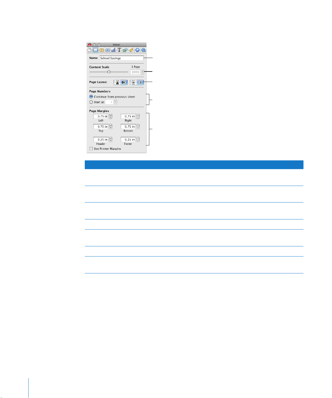
You set up page attributes, such as page orientation and margins, separately for each

Type a name for the sheet.

Shrink or enlarge all the sheet’s objects.

Set the page orientation and pagination order.

Set page margins.

Specify the sheet’s starting page number.

sheet, using the Sheet inspector.

To learn how to Go to

Set the page size to match the size of the paper you’ll be using

Have the header and footer text appear at the top and bottom of the table on each page

Adjust the size and location of objects on a sheet “Arranging Objects on a Page in Print View” on

Lay out pages horizontally or vertically “Setting Page Orientation” on page 42

Order pages from left to right or from top to bottom

Display page numbers in headers and footers “Numbering Pages” on page 42

Set up the blank space between the sheet’s edge and the edges of the paper

“Setting a Spreadsheet’s Page Size” on page 40

“Adding Headers and Footers to a Sheet” on page 41

page 41

“Setting Pagination Order” on page 42

“Setting Page Margins” on page 43

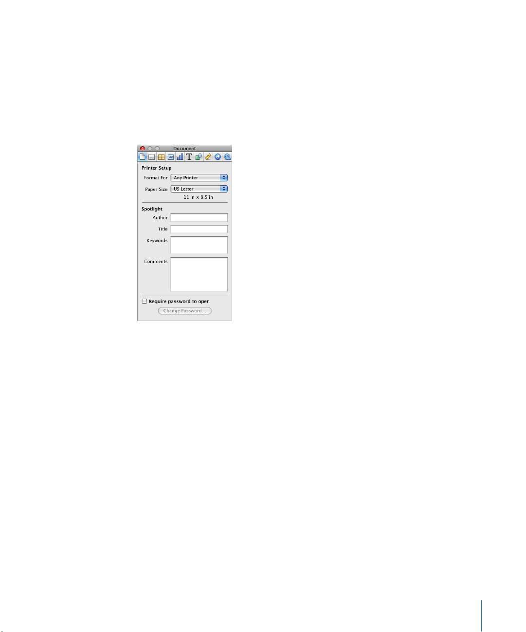
Setting a Spreadsheet’s Page Size

Before working with Print View, set the size of the pages to reect the size of the paper

1 Click inspector in the toolbar, and then click the Document inspector button.

2 Choose a page size from the Paper Size pop-up menu.

40 Chapter 2 Creating, Saving, and Organizing a Numbers Spreadsheet

you’ll be using.

To set the page size:

Adding Headers and Footers to a Sheet

You can have the same text appear on multiple pages in a sheet. Recurring information that appears at the top of the page is called a header; at the bottom it’s called a footer.

You can put your own text in a header or footer, and you can use formatted text

elds. Formatted text elds allow you to insert text that is automatically updated. For example, inserting the date eld shows the current date whenever you open the spreadsheet. Similarly, page number elds keep track of page numbers as you add or

delete pages.

To dene the contents of a header or footer:

1 Click View in the toolbar and choose Show Print View.

2 To see header and footer areas, hold the pointer near the top or bottom of a page.

You can also click View in the toolbar and choose Show Layout.

3 To add text to a header or footer, place the insertion point in the header or footer and

insert text.

4 To add page numbers or other changeable values, see the instructions in “Inserting

Page Numbers and Other Changeable Values” on page 186.

Arranging Objects on a Page in Print View

Resize objects, move them around on a page or between pages, and break up long tables across pages when you’re viewing a sheet in Print View.

To show Print View, click View in the toolbar and choose Show Print View.

Here are ways to lay out objects on a selected sheet’s pages:

To adjust the size of all the objects in the sheet in order to change the number of m pages they occupy, use the Content Scale controls in the Sheet inspector.

You can also drag the Content Scale slider at the bottom left of the canvas to resize everything on a sheet.

To resize individual objects, select them and drag their selection handles or change m

the Size eld values in the Metrics inspector.

To resize a table, see “Resizing a Table” on page 48. To resize a chart, see “Resizing or Rotating a Chart” on page 141. To resize other objects, see “Resizing Objects” on page 217.

In Print View, header rows and header columns appear on each page if a table spans m more than one page.

Chapter 2 Creating, Saving, and Organizing a Numbers Spreadsheet 41

To avoid showing header rows or columns when a table spans pages, on the Table menu deselect “Repeat Header Rows on Each Page” or “Repeat Header Columns on Each Page.”

Move objects from page to page by dragging them or by cutting and pasting them. m

Setting Page Orientation

You can lay out pages in a sheet in a vertical orientation (portrait) or a horizontal orientation (landscape).

To set a sheet’s page orientation:

1 Click View in the toolbar and choose Show Print View.

2 Click Inspector in the toolbar, click the Sheet inspector button, and click the

appropriate page orientation button in the Page Layout area of the pane.

You can also click a page orientation button at the bottom left of the canvas.

Setting Pagination Order

In Print View, pages can be ordered from left to right or from top to bottom. This order determines how the document prints and exports to PDF.

To set pagination order:

Click Inspector in the toolbar, click the Sheet inspector button, and then click the top- m

to-bottom or left-to-right button in the Page Layout area of the pane.

Numbering Pages

You can display page numbers in a page’s header or footer.

To number a sheet’s pages:

1 Select the sheet.

2 Click View in the toolbar and choose Show Print View.

3 Click View in the toolbar and choose Show Layout so you can see the headers

and footers.

You can also see the headers and footers by holding the pointer over the top or bottom of a page.

4 Click into the rst header or footer to add a page number, following the instructions in

“Inserting Page Numbers and Other Changeable Values” on page 186.

5 Click Inspector in the toolbar, click the Sheet inspector button, and then specify the

starting page number.

To continue page numbers from the previously selected sheet, select “Continue from previous sheet.”

To start the sheet’s page numbers at a particular number, use the Start At eld.

42 Chapter 2 Creating, Saving, and Organizing a Numbers Spreadsheet

Setting Page Margins

In Print View, every sheet’s page has margins (blank space between the sheet’s edge and the edges of the paper). These margins are indicated onscreen by light gray lines, visible when you use layout view.

To set the page margins for a sheet:

1 Select the sheet in the Sheets pane.

2 Click View in the toolbar and choose Show Print View, and then click View in the

toolbar and choose Show Layout.

3 Click Inspector in the toolbar, and then click the Sheet inspector button.

4 To set the distance between the layout margins and the left, right, top, and bottom

sides of a page, enter values in the Left, Right, Top, and Bottom elds.

5 To set the distance between a header or a footer and the top or bottom edge of the

page, enter values in the Header and Footer elds.

To print the spreadsheet using the largest printing area possible with any printer you

use, select Use Printer Margins. Any margin settings specied in the Sheet inspector

are ignored when you print.

Chapter 2 Creating, Saving, and Organizing a Numbers Spreadsheet 43

Using Tables

This chapter explains how to add and format tables and their rows and columns.

Several other chapters provide instructions that focus on particular aspects of tables.

To learn how to Go to

Manage table cells and content in them Chapter 4, “ Working with Table Cells,” on page 75

Use table styles to format tables Chapter 5, “ Working with Table Styles,” on

page 111

Use formulas in table cells Chapter 6, “Using Formulas in Tables,” on page 115

Display table cell values in charts Chapter 7, “Creating Charts from Data,” on

page 131

Working with Tables

Use a variety of techniques to create tables and manage their characteristics, size, and location.

To learn how to Go to

Insert tables “Adding a Table” on page 45

Use table tools “Using Table Tools” on page 45

Make tables larger or smaller “Resizing a Table” on page 48

Relocate tables “Moving Tables” on page 48

Assign names to tables “Naming Tables” on page 49

Apply color and other visual eects to tables “Enhancing the Appearance of Tables” on page 49

Dene tables you can use again and again “Dening Reusable Tables” on page 50

Share tables among iWork applications “Copying Tables Among iWork Applications” on

page 51

Adding a Table

Arrange text in table cells.

Format cell borders.

Add background

color to a cell.

Format cell values.

Manage headers

and footers.

Show or hide a table’s name.

Format text in

table cells.

While most templates contain one or more predened tables, you can add tables to

your Numbers spreadsheet.

Here are ways to add a table:

Click Tables in the toolbar and choose a predened table from the pop-up menu. m

You can add your own predened tables to the pop-up menu. See “Dening Reusable

Tables” on page 50 for instructions.

Choose Insert > Table > m type of table.

To create a new table based on one cell or several adjacent cells in an existing table, m select the cell or cells and then drag the selection to an empty location on the sheet. To retain values in the selected cells in the original table, hold down the Option key while dragging.

See “Selecting Tables and Their Components” on page 51 to learn about cell selection techniques.

To create a new table based on an entire row or column in an existing table, click the m reference tab associated with the row or column, press the reference tab, drag the row or column to an empty location on the sheet, and then release the tab. To retain values in the column or row in the original table, hold down the Option key while dragging.

Using Table Tools

You can format a table and its columns, rows, cells, and cell values using various Numbers tools.

Here are ways to manage table characteristics:

Select a table by clicking its name in the Sheets pane, and use the format bar to m quickly format the table. “Selecting a Table” on page 52 describes other ways to select a table.

Chapter 3 Using Tables 45

Use the Table inspector to access table-specic controls, such as elds for precisely m

Add a table name.

Merge or split

selected cells.

Adjust the size of rows and columns.

Set the style, width, and color of cell borders.

Add color or an image to a cell.

Change the behavior

of the Return and

Tab keys.

Add or remove 1-5 header rows, header columns, and footer rows.

The buttons at the top of the inspector window open the ten inspectors: Document, Sheet, Table, Cells, Chart, Text, Graphic, Metrics, Hyperlink, and QuickTime.

controlling column width and row height. To open the Table inspector, click Inspector in the toolbar, and then click the Table inspector button.

Use the Cells inspector to format cell values. For example, you can display a currency m symbol in cells containing monetary values. Cell formats determine how cell values are displayed, but they never change the underlying cell value used in calculations. For example, a cell with the actual value of 4.29 might be displayed as 4.3, but calculations use the value 4.29.

You can also set up conditional formatting. For example, you can make a cell red when its value exceeds a particular number.

To open the Cells inspector, click Inspector in the toolbar, and click the Cells inspector button.

46 Chapter 3 Using Tables

Use the Graphic inspector to create special visual eects, such as shadows. To open m

Drag the Table handle to move the table.

Reference tab letters can be used to refer to columns.

Click the Column handle to add one column. Drag it to add multiple columns.

Reference tab

numbers can

be used to

refer to rows.

Drag the Column and Row handle down to add rows. Drag it to the right to add columns. Drag it diagonally to add rows and columns at the same time.

Click the Row handle to add one row. Drag it to add more rows.

the Graphic inspector, click Inspector in the toolbar and then click the Graphic inspector button.

Use table styles to adjust the appearance of tables quickly and consistently. See m “Using Table Styles” on page 111 for more information.

Use the reference tabs and handles that appear when you select a table cell to quickly m reorganize a table, select all the cells in a row or column, add rows and columns, and more. “Selecting a Table Cell” on page 52 describes how to select a table cell.

You also use reference tabs when you work with formulas (“Referring to Cells in Formulas” on page 12 3 explains how).

Access a shortcut menu by selecting a table or one or more cells and then holding m down the Control key as you click again.

You can also use the pop-up menus on the column and row reference tabs.

Chapter 3 Using Tables 47

Use the Formula Editor and formula bar to add and edit formulas. See “ m Adding and Editing Formulas Using the Formula Editor” on page 119 and “Adding and Editing Formulas Using the Formula Bar” on page 12 0 for details.

Use the Function Browser to add and edit functions. See “ m Adding Functions to Formulas” on page 121 for details.

Resizing a Table

You can make a table larger or smaller by dragging one of its selection handles or by using the Metrics inspector. You can also change the size of a table by resizing its columns and rows.

Before resizing a table, select it by clicking its name in the Sheets pane or using one of the other techniques in “Selecting a Table” on page 52.

Here are ways to resize a selected table:

Drag one of the square selection handles that appear when a table is selected. m

To maintain a table’s proportions, hold down the Shift key as you drag.

To resize from the table’s center, hold down the Option key as you drag.

To resize a table in one direction, drag a side handle instead of a corner handle.

To resize by specifying exact dimensions, select a table or table cell, click Inspector in m the toolbar, and then click the Metrics inspector button. Using the Metrics inspector, you can specify a new width and height, and you can change the table’s distance from

the margins by using the Position elds.

To resize by adjusting the dimensions of rows and columns, see “ m Resizing Table Rows and Columns” on page 62.

Moving Tables

You can move a table by dragging it, or you can relocate a table using the Metrics inspector.

Here are ways to move a table:

If the table isn’t selected or if the entire table is selected, press the edge of the table m and drag it.

If a table cell is selected, drag the table using the Table handle in the upper left.

48 Chapter 3 Using Tables

To constrain the movement to horizontal, vertical, or 45 degrees, hold down the Shift m key as you drag.

To move a table more precisely, click any cell, click Inspector in the toolbar, click the m

Metrics inspector button, and then use the Position elds to relocate the table.

To copy a table and then move the copy, hold down the Option key, press at the edge m of an unselected table or an entire table that’s selected, and drag.

Naming Tables

Every Numbers table has a name that’s displayed in the Sheets pane and can optionally be displayed above the table. The default table name (Table 1, Table 2, and so forth) can be changed, hidden, and formatted.

Here are ways to work with table names:

To change the name, double-click it in the Sheets pane and type the new name. m

You can also click in the table and change its name using the Table inspector’s

Name eld.

On any sheet, two tables can’t have the same name.

To show a table’s name on the sheet canvas, click in the table and then select Name in m the format bar or the Table inspector.

To hide the table name on the sheet, deselect Name.

To format a name displayed on the sheet canvas, select the table, click the table name m on the sheet canvas to activate the name for formatting, and use the format bar, Fonts window, or Text pane of the Text inspector.

To increase the distance between the table name and the table body, select Name in m the Table inspector, click the name on the canvas, and then use the Text inspector to modify the After Paragraph spacing.

Enhancing the Appearance of Tables

You can apply color, use images, and use other formatting techniques to enhance the visual appeal of your tables.

Here are ways to enhance a table’s appearance:

You can ll the background of an entire table or individual cells with dierent kinds of m color eects or with an image. See “Filling Objects with Colors or Images” on page 223

for instructions.

You can change the thickness and color of borders around a table and its cells, as m “Formatting Table Cell Borders” on page 84 describes.

You can adjust the attributes of text in table cells, including header and footer cells. m See “Formatting Text Size and Appearance” on page 16 3 and “Setting Text Alignment, Spacing, and Color” on page 170 for details.

Chapter 3 Using Tables 49

When you’ve created a visual eect that you want to reuse, you can copy and paste it; select the table or cells whose eects you want to reuse, choose Format > Copy Style,

select the table or cells you want to format, and then choose Format > Paste Style. You can also use table styles to replicate formatting you’ve applied to a table, as “Using Table Styles” on page 111 describes.

Dening Reusable Tables

You can add your own tables to the menu of predened tables that appears when

you click Tables in the toolbar or choose Insert > Table. Reusable tables have the table style and structure of your choice and can contain content (header text, formulas, and so on).

To dene a reusable table:

1 Select a table.

2 Dene a table style for the table.

The table style determines the formatting of borders, background, and text in the table’s cells.

One way to dene the table style is by following the instructions in “Modifying Table Style Attributes” on page 11 2 and “Copying and Pasting Table Styles” on page 113 .

Alternatively, you can apply your customized table structure and content to the reusable table, but give it the table’s original default style instead of your own. Step 7 describes how to use this option.

3 Dene the table’s structure.

To resize the table, see “Resizing a Table” on page 48 and “Resizing Table Rows and Columns” on page 62.

To dene columns and rows, see “Working with Rows and Columns in Tables” on page 55.

To split or merge table cells, see “Splitting Table Cells” on page 84 or “Merging Table Cells” on page 83.

4 Add and format any content you want to reuse. See “Putting Content into Table

Cells” on page 75 for instructions. Any formulas you add should refer only to cells in

the table you’re dening.

5 Choose Format > Advanced > Capture Table.

6 Type a name for the table.

7 Select “Use the default style from the document” if you want the table to be styled

using the default table style in eect when the table is added to the spreadsheet. Otherwise the table style used is the one you dened in step 2.

8 Click OK.

50 Chapter 3 Using Tables

A copy of your reusable table can now be added to the current spreadsheet by choosing it from the menu of predened tables that appears when you click Tables in the toolbar or choose Insert > Table.

To rearrange, rename, or delete tables on the menu, choose Format > Advanced >

Manage Tables. Double-click a name to change the name of a predened table. Select

a table and click the up or down arrow button to move it up or down in the list of

tables. Click the Delete (–) button to remove a table. Click Done when you’ve nished.

The table and menu changes apply only to the current spreadsheet. If you want your reusable tables and menu changes to be available in other spreadsheets, save the spreadsheet as a template, using the instructions in “Saving a Custom Template” on page 246.

Copying Tables Among iWork Applications

You can copy a table from one iWork application to another.

The table retains its appearance, data, and other attributes, but some Numbers features aren’t supported in the other applications:

Rows or columns that are hidden in Numbers are removed. Â

Comments added to Numbers table cells aren’t copied. Â

To copy a table from one iWork application to another:

1 Select the table you want to copy, as “Selecting a Table” on page 52 describes.

2 Choose Edit > Copy.

3 In the other application, set an insertion point for the copied table, and then choose

Edit > Paste.

Selecting Tables and Their Components

You select tables, rows, columns, table cells, and table cell borders before you work with them.

To learn how to Go to

Select tables “Selecting a Table” on page 52

Select a table cell “Selecting a Table Cell” on page 52

Select a group of table cells “Selecting a Group of Table Cells” on page 53

Select a row or a column “Selecting a Row or Column in a Table” on

page 54

Select cell borders “Selecting Table Cell Borders” on page 54

Chapter 3 Using Tables 51

Selecting a Table

When you select a table, selection handles appear on the edges of the table.

Here are ways to select a table:

Click the table name in the Sheets pane. m

If a table cell isn’t selected, move your pointer to the edge of the table. When the m pointer changes to include a black cross, you can click to select the table.

If a table cell or border segment is selected, click the Table handle in the upper left to m select the table. You can also press Command-Return.

Selecting a Table Cell

When you select a cell, the border of the selected cell is highlighted.

Selecting a cell also displays reference tabs along the top and sides of the table.

To select a single table cell:

1 Move the pointer over the cell. The pointer changes into a white cross.

2 Click the cell.

When a cell is selected, use the Tab, Return, and arrow keys to move the selection to an adjacent cell. Deselecting “Return key moves to next cell” below Table Options in the

Table inspector changes the eect of the Return and Tab keys. Deselect the checkbox

if you want the Return key to act like a carriage return within the cell, which is most useful when you type paragraphs of text in a cell.

52 Chapter 3 Using Tables

To select If “Return key” option is

selected

The next cell to the right Press Tab.

If you press Tab when the last cell in a column is selected, a new column is added.

If you add or change data in the last column, press Tab twice to add a new column.

The previous cell Press Shift-Tab. Press Shift-Tab.

The next cell down Press Down Arrow or Return.

If you’ve been using the Tab key to navigate between cells, pressing Return selects the next cell down from the cell in which you started tabbing.

If you press Return when the last cell in a row is selected, a new row is added.

If you add or change data in the last cell, press Return twice to add a new row.

The next cell up Press Up Arrow or Shift-Return. Press Up Arrow or Shift-Return.

If “Return key” option isn’t selected

Press Tab.

If you press Tab in the last

column, the rst cell in the next

row is selected.

If you press Tab in the last cell of the table, a new row is added.

If you press Shift-Tab in the rst

cell, the last cell is selected.

Press Down Arrow.

Selecting a Group of Table Cells

You can select adjacent or nonadjacent cells.

Here are ways to select a group of cells:

To select adjacent table cells, select a single cell, and then hold down the Shift key as m you select adjacent cells.

You can also click a cell, press, and then drag through a range of cells.

To select nonadjacent table cells, hold down the Command key as you select cells. m Use Command-click to deselect a cell in the group.

Chapter 3 Using Tables 53

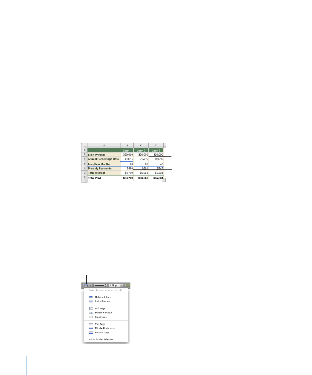
Selecting a Row or Column in a Table

A single (horizontal) border segment

A long (vertical) border segment

A long (horizontal) border segment

A single (vertical) border segment

Borders button

Select rows and columns using their reference tabs.

To select an entire row or column:

1 Select any table cell so that the reference tabs are showing.

2 Do one of the following:

Select a column by clicking its reference tab (above the column). Â

Select a row by clicking its reference tab (to the left of the row). Â

Selecting Table Cell Borders

Select cell border segments when you want to format them or drag them to resize rows and columns. A single border segment is one side of a cell. A long border segment includes all adjacent single border segments.

After selecting border segments, you can format their color and stroke, as “Formatting Table Cell Borders” on page 84 describes, or drag them to make rows and columns larger or smaller, as “Resizing Table Rows and Columns” on page 62 describes.

Here are ways to select border segments:

To quickly select border segments for formatting, select a table, row, column, or cell. m

Click the Borders button in the format bar, and choose an option from the pop-up menu.

54 Chapter 3 Using Tables

You can also use the Cell Borders buttons in the Table inspector to select

The pointer looks like this when it’s over a horizontal segment.

The pointer looks like this when it’s over a vertical segment.

a border segment.

To select border segments for either formatting or resizing rows and columns, use m border selection mode. Choose Allow Border Selection from the Borders pop-up menu in the format bar or choose Table > Allow Border Selection, and then select the table you want to work with.

The pointer changes shape when it’s over a horizontal or vertical segment. The pointer appears to straddle the segment.

To select a long segment, click a cell’s horizontal or vertical border. To change the selection to a single segment, click it again.

To add a single or long segment to the selection, hold down the Shift or Command key while clicking.

To deselect a selected single segment, click it while holding down the Shift or Command key.

To go back and forth between single-segment and long-segment selection, click a border.

To stop using border selection mode, choose Disallow Border Selection from the Borders

pop-up menu in the format bar or choose Table > Disallow Border Selection.

Working with Rows and Columns in Tables

You can quickly add or remove rows and columns, create header rows or columns or footer rows, and more.

When you insert, remove, resize, hide, or show rows or columns in a table, other objects on the sheet may be moved to avoid overlapping or to maintain relative object positions. To prevent automatic movement of objects, choose Numbers > Preferences and in the General pane deselect “Automatically move objects when tables resize.”

To learn how to Go to

Insert new rows into a table “Adding Rows to a Table” on page 56

Insert new columns into a table “Adding Columns to a Table” on page 57

Move or copy rows and columns to a dierent location in the same or a dierent table

Chapter 3 Using Tables 55

“Rearranging Rows and Columns” on page 58

To learn how to Go to

Delete rows and columns “Deleting Table Rows and Columns” on page 58

Use header rows and header columns “Adding Table Header Rows or Header

Columns” on page 59

Freeze header rows and columns so they remain in view as you scroll through a table’s body rows and body columns

Use footer rows “Adding Table Footer Rows” on page 61

Resize rows and columns “Resizing Table Rows and Columns” on page 62

Give every other row in a table a dierent

background color

Hide selected rows and columns “Hiding Table Rows and Columns” on page 63

Sort rows in ascending or descending order using the value of cells in one or more columns

Hide rows that don’t contain particular values “Filtering Rows in a Table” on page 65

Arrange rows into categories and subcategories to highlight characteristics they share

“Freezing Table Header Rows and Header Columns” on page 60

“Alternating Table Row Colors” on page 62

“Sorting Rows in a Table” on page 64

“Creating Table Categories” on page 66

“Dening Table Categories and Subcategories” on page 67

“Removing Table Categories and Subcategories” on page 72

“Managing Table Categories and Subcategories” on page 72

Adding Rows to a Table

You can add rows within a table or at the end of a table.

If the table contains a footer row, rows added at the bottom of the table are added

above the footer row. If the table has ltering criteria associated with it, you can’t add new rows until you stop ltering rows; see “Filtering Rows in a Table” on page 65 for

instructions.

If all the body cells in a column above the new row contain the same formula or cell control, the formula or cell control is repeated in the new row.

Here are ways to add rows:

To add a row above a selected cell, press Option-Up Arrow. m

To add a row below a selected cell, press Option-Down Arrow.

You can add a single row above or below a particular row by holding the pointer over m a row’s reference tab to see its menu arrow, clicking the arrow, and then choosing Add Row Above or Add Row Below from the pop-up menu.

56 Chapter 3 Using Tables

You can also click in a row and then choose Table > Add Row Above or Table > Add Row Below.

To add multiple rows, select the number of rows you want to add (select three rows if m you want to add three rows). To add rows after a particular row, make sure the bottom row selected is the one after which you want the new rows added; to add rows before a particular row, make sure the top row selected is the one before which you want the new rows added. Then choose Table > Add Rows Above or Table > Add Rows Below.

To add a row at the end of the table, press Return while the last cell is selected. m Press Return twice if you’ve just added or changed the cell value and you’re still editing the cell.

If “Return key moves to next cell” below Table Options in the Table inspector isn’t selected, press Tab instead from the last cell in the row.

To add one or more rows at the end of the table, you can use the Row handle in the m lower left, visible when a cell is selected.

To add a row at the end of the table, click the Row handle once.

To add multiple rows at the end of the table, drag the Row handle or the Column and

Row handle (in the lower right) down.

To add rows and columns at the same time, drag the Column and Row handle diagonally.

You can split cells into two equal rows. “ m Splitting Table Cells” on page 84 describes how.

Adding Columns to a Table

Here are ways to add columns:

To add a column after a selected cell, press Option-Right Arrow. m

To add a column before a selected cell, press Option-Left Arrow.

To add a single column, hold the pointer over a column’s reference tab to see its menu m arrow. Click the arrow and then choose Add Column Before or Add Column After from the pop-up menu. You can also select a column and then choose these commands from the Table menu.

To add multiple columns, select the number of columns you want to add (select three m columns to add three columns). To add columns after a particular column, make sure the rightmost column selected is the one after which you want the new columns added; to add columns before a particular column, make sure the leftmost column selected is the one before which you want the new columns added. Then choose one of the commands above.

You can use the Tab key to add a column to the right side of the table when “Return m key moves to next cell” below Table Options in the Table inspector is selected.

Chapter 3 Using Tables 57

Press Tab once when the last cell is selected. Press Tab twice if you’ve just added or changed the cell value and you’re still editing the cell.

To add one or more columns to the right side of a table, you can use the Column handle in the upper right, visible when a cell is selected.

To add a column to the right side of the table, click the Column handle once.

To add multiple columns to the right side of the table, drag the Column handle or the

Column and Row handle (in the lower right) to the right.

To add rows and columns at the same time, drag the Column and Row handle diagonally.

You can split cells into two equal columns. “ m Splitting Table Cells” on page 84 explains how.

Rearranging Rows and Columns

Using a row’s or column’s reference tab, you can move or copy the row or column to

a dierent location in the same table or another table.

Here are ways to rearrange rows and columns:

To move a column or row to a dierent location in the same table or a dierent table, m

click the column or row reference tab, press, and then drag the reference tab. Release the tab when the bold line highlights where you want to insert the column or row.

To insert a copy of a row or column elsewhere in the table or in another table, click m the reference tab, and then press and hold down the Option key and the reference tab while you drag the column or row to the desired location.

You can also copy or move a single cell or a group of adjacent cells within or between tables. See “Copying and Moving Cells” on page 85 for instructions.

Deleting Table Rows and Columns

There are several techniques available for deleting one or more rows or columns of a table.

Here are ways to delete rows or columns:

Select one or more rows or columns or a cell in a row or column, and then choose m Table > Delete Row or Table > Delete Column.

To delete a single row or column, hold the pointer over the row or column reference m tab to see the menu arrow, and then choose Delete Row or Delete Column from the pop-up menu.

To delete several adjacent rows or columns, select the rows or columns and then m choose Delete Selected Rows or Delete Selected Columns from the pop-up menu of a selected row’s or column’s reference tab.

58 Chapter 3 Using Tables

To delete empty rows, drag the lower-left Row handle up or drag the lower-right m Column handle up.

To remove rows with content, hold down the Option key while dragging.

To delete empty columns, drag the upper-right Column handle inward. m

To remove columns with content, hold down the Option key while dragging.

Adding Table Header Rows or Header Columns

Use header rows and columns when you want to label rows and columns. Header rows and columns are formatted so that they stand out from the other (body) rows and columns. Header rows are always directly above the topmost body row. Header columns are always directly to the left of the leftmost body column.

You can use as many as ve header rows and ve header columns. Multiple headers

are useful when you want to assign names to two or more header columns or header rows. To format a header to span rows or columns, merge the header cells, as “Merging Table Cells” on page 83 describes.

If a table contains both header rows and header columns, the top left cell or cells are considered to be part of the header row. Header columns appear below any header rows.

Header rows and header columns can be set to appear at the beginning of the table and on each page if the table spans more than one page. In Print View, click the appropriate header button in the format bar and choose “Repeat Header Rows on Each Page.” If a table spans multiple pages, editing the text or changing the look of a header row or column in one place changes it consistently throughout the table.

To learn about Print View, see “ Â Dividing a Sheet into Pages” on page 39.

To learn about keeping headers in view when not working in Print View, see Â “Freezing Table Header Rows and Header Columns” on page 60.

Here are ways to add or delete header rows or header columns:

If a table has no headers, select the table and click a Header button in the format bar m to add one.

Click it again to remove the header.

Chapter 3 Using Tables 59

Click the disclosure triangle next to a Header button in the toolbar, and then choose m

Add header column.

Add header rows.

the number of header rows or header columns to add from the pop-up menu. Choose 0 to remove all header rows or header columns.

To delete a header row or header column, hold the pointer over the reference tab m of a header row or header column to see its menu arrow. Click the arrow and then choose Delete Row or Delete column from the pop-up menu.

Select a table or an element in it. Click Inspector in the toolbar, click the Table m inspector button, and then click the appropriate Headers & Footer button. Choose the number of header rows or header columns from the pop-up menu.

Select a table or an element in it and then choose Table > Header Rows or Table > m Header Columns. Then choose the number of header rows or header columns from the submenu.

Convert the topmost body row or the leftmost body column to a header row or m header column. Hold the pointer over the reference tab of a body row or column to see its menu arrow. Click the arrow and then choose Convert to Header Row or Convert to Header Column from the pop-up menu. These commands are available only when there are four or fewer existing header rows or header columns.

Header cells play an important role in making formulas in table cells easier to read and create. See “Referring to Cells in Formulas” on page 12 3 to learn more.

Freezing Table Header Rows and Header Columns

When you’re not in Print View (which repeats header rows and columns on each page), you can keep headers visible as you scroll through the document by using the freeze option.

Here are ways to freeze and unfreeze header rows and columns for a table:

Select the table or an element in it, click the row header or column header button in m the format bar, and then select or deselect Freeze Header Columns or Freeze Header Rows in the pop-up menu.

You can also access these commands from the header buttons in the Table inspector.

60 Chapter 3 Using Tables

Select the table or an element in it, and choose Table > Header Columns or Table > m Header Rows. Then select or deselect Freeze Header Columns or Freeze Header Rows.

Adding Table Footer Rows

Add footer rows.

Use footer rows when you want to draw attention to the bottom rows of a table. Footer rows are formatted so that they stand out from the other (body) rows. A footer row consists of the bottommost cell in each column.

You can use as many as ve footer rows. To format a footer to span columns, merge

the footer cells, as “Merging Table Cells” on page 83 describes.

Here are ways to add or delete footer rows:

If a table has no footers, select the table and click the Footer button in the format bar m to add one.

Click it again to remove the footer.

Click the disclosure triangle next to the Footer button in the toolbar, and then choose m the number of footer rows to add from the pop-up menu. Choose 0 to remove all footer rows.

To delete a footer row, hold the pointer over the reference tab of a footer row to see its m menu arrow, and then click the arrow and choose Delete Row from the pop-up menu.

Select a table or an element in it. Click Inspector in the toolbar, click the Table m inspector button, and then click the Footer button. Choose the number of footer rows from the pop-up menu.

Select a table or an element in it and then choose Table > Footer Rows. Then choose m

Chapter 3 Using Tables 61

the number of footer rows from the submenu.

Resizing Table Rows and Columns

Resize all rows and columns so they’re equal in size, or resize only specic rows and

columns in a table.

Here are ways to resize rows and columns:

To make all rows the same size, select the table or one or more columns, and then m choose Table > Distribute Rows Evenly.

To make all columns the same size, select the table or one or more rows, and then m choose Table > Distribute Columns Evenly.

To resize a single row, drag the bottom border of the row’s reference tab up or down. m

You can also select the row and use the Row Height eld in the Table inspector.

To resize one column, drag the right border of the column’s reference tab right or left. m

You can also select a cell and use the Column Width eld in the Table inspector.

To make several rows the same size, select one or more cells in the rows and choose m Table > Distribute Rows Evenly. The rows don’t have to be adjacent.

You can also drag the bottom border of the reference tab of one of the rows up or

down or use the Row Height eld in the Table inspector.

To make several columns the same size, select one or more cells in the columns and m choose Table > Distribute Columns Evenly. The columns don’t have to be adjacent.

You can also drag the right border of the reference tab of one of the columns left or

right or use the Column Width eld in the Table inspector.

To shrink a row or column to remove unused space when cell values don’t ll their m

cells, select a cell and click one of the Fit buttons in the Table inspector. You can also double-click a column or row reference tab separator.

If cell content is clipped as a result of resizing, see “Displaying Content Too Large for Its Table Cell” on page 79 for options.

To resize columns or rows by dragging border segments, choose Allow Border m Selection from the Borders pop-up menu in the format bar or choose Table > Allow Border Selection.

Select the table, and then click and drag a horizontal or vertical border.

Alternating Table Row Colors

Use a dierent color background for alternate rows to give a table a banded eect.

To alternate row colors:

1 Select the table or an element in it.

2 Click Inspector in the toolbar and then click the Table inspector button.

3 Select Alternating Row Color.

62 Chapter 3 Using Tables

4 Click the adjacent color well to open the Colors window, and then choose a color for

the alternate rows. See “The Colors Window” on page 24 for instructions.

5 To change the ll attributes of the other rows, use the Cell Background controls in the

Table inspector. See “Filling Objects with Colors or Images” on page 223 for instructions.

Hiding Table Rows and Columns

Hide specic rows or columns when you want to avoid showing or using them but

don’t want to delete them. While a row or column is hidden, it can’t be reformatted, merged, split, or otherwise manipulated. However, any formula that uses a hidden cell

isn’t aected, and sorting takes hidden values into account.

When a row or column is hidden, you’ll see a gap in the row numbers or column letters in the reference tabs.

Here are ways to hide and show rows and columns:

To hide a single row or column, choose Hide Row or Hide Column from the row or m column reference tab’s pop-up menu.

To hide multiple rows or columns, select the rows or a cell in each of them and then choose Hide Selected Rows or Hide Selected Columns from a reference tab pop-up menu.

To show all hidden rows and columns in a table, select the table or an element in it m and then choose Table > Unhide All Rows or Table > Unhide All Columns.

You can also choose these commands from any reference tab’s pop-up menu.

Chapter 3 Using Tables 63

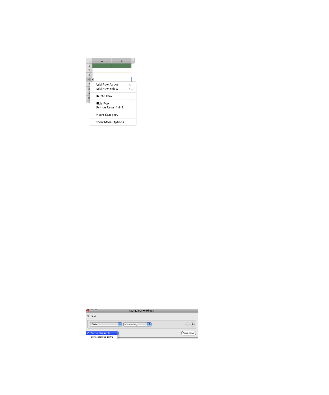
To show rows hidden immediately above a row or columns hidden immediately m to the left of a column, click the reference tab for the row or column and then choose “Unhide Rows row numbers“ or “Unhide Columns column letters” from the pop-up menu.

To show rows or columns hidden in a selected range of rows or columns, select the m range and then choose Unhide Selected Rows from the pop-up menu of any of the selected rows or columns.

Rows or columns that are hidden in Numbers tables are removed when the tables are copied into other iWork applications.

Rows and columns that contain merged cells can’t be hidden.

Sorting Rows in a Table

You can arrange values in some or all the cells in a column in ascending or descending order. Rows containing cells being sorted are reordered. Header cells aren’t sorted.

Sorting takes into account values in hidden rows and hidden columns.

Here are ways to sort:

To sort an entire table by reordering cells in a column, choose Sort Ascending or Sort m Descending from the pop-up menu for the column’s reference tab.

You can also click in a table and then click Reorganize in the toolbar or choose Show More Options from a reference tab’s pop-up menu to open the Reorganize window. Click the Sort disclosure triangle to reveal the sort controls. Choose “Sort entire table” from the pop-up menu, and then choose a column and sort order from the other pop-up menus.

64 Chapter 3 Using Tables

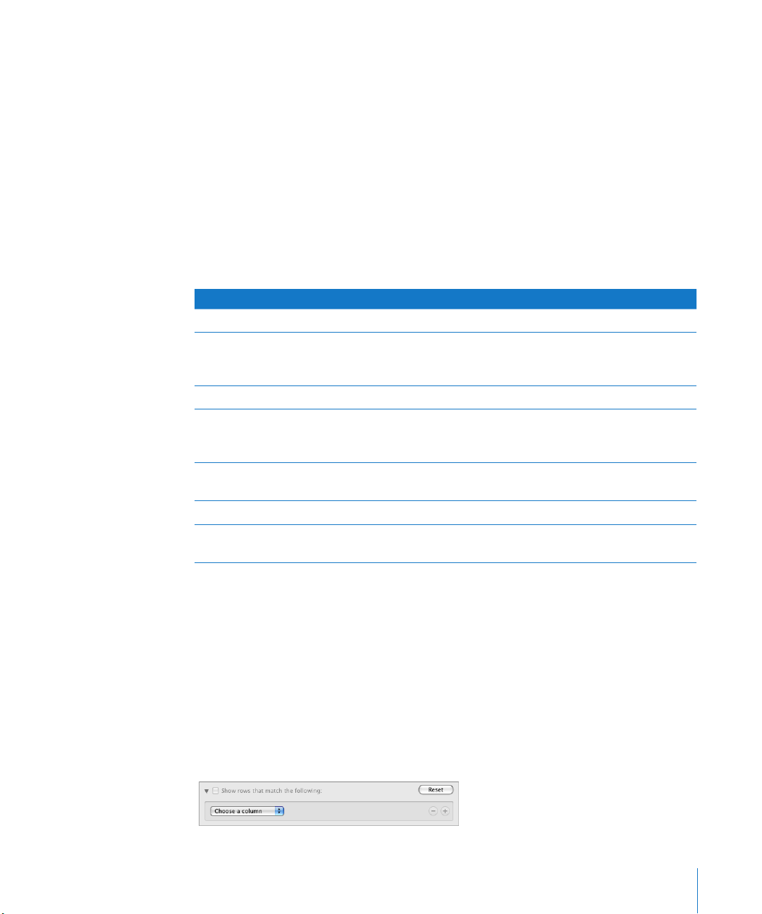
To sort only part of a table, select the rows you’d like to sort, open the Reorganize m window, and choose “Sort selected rows” from the pop-up menu. Then choose a column to sort by and a sort order from the other pop-up menus.

To re-sort values after changing them, open the Reorganize window and click m Sort Now.

To sort the table by one column and then by another column, open the Reorganize m window and choose an option from the three pop-up menus. Then click the Add button (+) and choose options for the second sort.

To apply additional sort criteria, click the Add button (+) again.

The following table describes how dierent types of data are sorted in ascending or

descending order.

Type of data Ascending order Descending order

Tex t aA–zZ Zz–Aa

Dates Year (earliest rst), then month

(January rst), then day (1–31)

Numbers –2, –1, 0, 1, and so on 1, 0, –1, –2, and so on

Cells containing only text, mixed with cells containing only numbers

Cells containing a mixture of text and numbers

Empty cells At the bottom At the bottom

Boolean (TRUE, FALSE) Below text and above an empty

–2, –1, 0, 1, and so on, then aA–zZ

Values starting with numbers

rst (1z, 1Z, a1, A1)

cell

Year (most current rst), then month (December rst), then

day (31–1)

Zz–Aa, then 1, 0, –1, –2, and so on

Values starting with text rst

(A1, a1, 1A, 1z)

Above text

Filtering Rows in a Table

You can hide rows in a table that don’t contain the values you specify.

When you sort table cells, values in hidden rows are taken into account.

To specify criteria for rows you want to show:

1 Click in the table.

2 Click Reorganize in the toolbar or choose Show More Options from a reference tab’s

pop-up menu to open the Reorganize window.

3 Click the Filter disclosure triangle to reveal the ltering controls.

Chapter 3 Using Tables 65

4 Choose the column whose values you want to use to create lter criteria.

Category row for office furniture

Category row for patio furniture

Category row for library furniture

Cell reference

pop-up menu for this

category row

5 Use the remaining controls to dene the column value for rows you want to show.

6 To use additional lter criteria, click the Add button (+) to dene each one you want

to add.

If you choose “is in the top n values” or “is in the bottom n values,” all values matching the top or bottom n will be shown, which may be more than n.

Note: You can’t add any new rows to the table until you stop ltering rows. To stop ltering rows in the table, deselect “Show rows that match the following” in the

Reorganize window.

Creating Table Categories

You can organize a table into categories. You can create categories by selecting particular rows for a category, or you can set Numbers to create categories and subcategories automatically using the value in one or more columns of the table (category value columns). When you use category value columns, changing values

in them may cause rows to move into dierent categories.

Each category or subcategory is displayed with a category row above it. You click the disclosure triangle near the left edge of the category row to view or hide (expand or collapse) the category.

Category rows have special characteristics that help you manage your categories.

You can add new categories, remove categories, and perform other operations by Â using the cell reference pop-up menu for a category row. Choosing Expand All or Collapse All expands or collapses all categories at the level of the row from which you chose the command.

66 Chapter 3 Using Tables

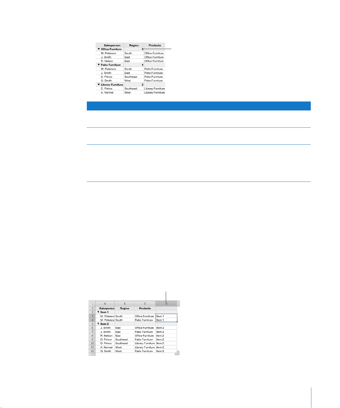
You can display automatically calculated values (such as subtotals and row count) in Â

Calculated row count

Category value column

category row cells.

To learn how to Go to

Create categories and subcategories “Dening Table Categories and Subcategories” on

page 67

Remove categories “Removing Table Categories and

Subcategories” on page 72

Add or remove rows from categories, display automatically computed values in cells of a category row, move a category, change the level of a category, collapse or expand category rows, and perform other category management tasks

“Managing Table Categories and Subcategories” on page 72

Dening Table Categories and Subcategories

You can have Numbers create categories or subcategories based on values in one or more columns in the table. Or you can assemble rows into categories by manually inserting category rows between table rows. You can create categories based on adjacent or nonadjacent selected table rows.

Creating categories manually

When you create categories by manually inserting a category row, a new column (the category value column) is added to the table to display unique placeholder values for each category. The placeholder value is used in the category row to identify the category.

Chapter 3 Using Tables 67

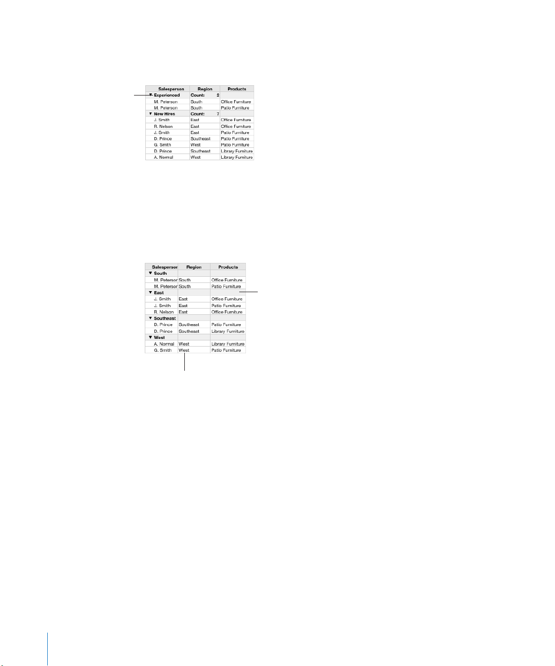
You may want to hide the column (click its reference tab’s pop-up menu and

Double-click to type

a new category name.

Category row

Category value column

choose Hide Column). To change the placeholder name in a category row to a more meaningful name, edit the name as you would text in any cell.

Creating categories using values in a column

When you categorize a table using the values in a column, Numbers creates a dierent

category for each unique value in the column. The column whose value you use to create categories is the category value column. All rows containing the same value in the category value column are placed together in a category. The shared value is used as the category name in the category row.

If you change a value in the category value column, the row moves into a dierent

category if the value exists elsewhere in the category value column; otherwise, a new category is created for the new value.

You can optionally hide a category value column, but you may want to leave the column visible in case you need to change values in it. Also, you may not want to edit the name in the category row. When you change a category row’s name, all the values in the category value column for the category are replaced with the new name, overwriting other values in the cells.

Here are ways to create categories and subcategories:

To divide a table’s rows at a particular place, choose Insert Category from the reference m tab pop-up menu for the bottommost row in the category you want to create. For

example, to divide a 9-row table into two categories with the rst 5 rows in the rst

category, choose Insert Category from the pop-up menu for row 5.

68 Chapter 3 Using Tables

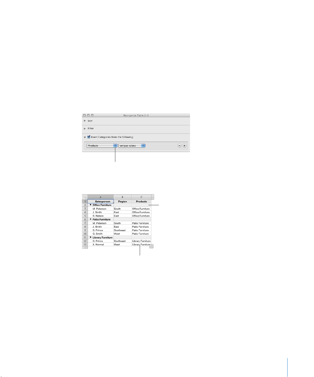
To place a range of adjacent or nonadjacent rows into a category, select the rows and m

Choose the name of the column you want to use as a category value column.

Category row

Category value column

then choose “Create Category from Selected Rows” from the reference tab’s pop-up menu for one of the selected rows.

To categorize rows with the same value in a particular column, choose “Categorize by m This Column” from the reference tab pop-up menu for the column. When a value in the

column changes, its row is placed in a dierent category based on its new cell value.

You can also use the Reorganize window. Click in the table and then click Reorganize in the toolbar or choose Show More Options from a reference tab’s pop-up menu to open the Reorganize window. Click the Categories disclosure triangle to reveal the

categorizing controls. From the rst pop-up menu, choose the name of the column

you want to use as a category value column.

Table categories are created based on unique values in the chosen column.

Chapter 3 Using Tables 69

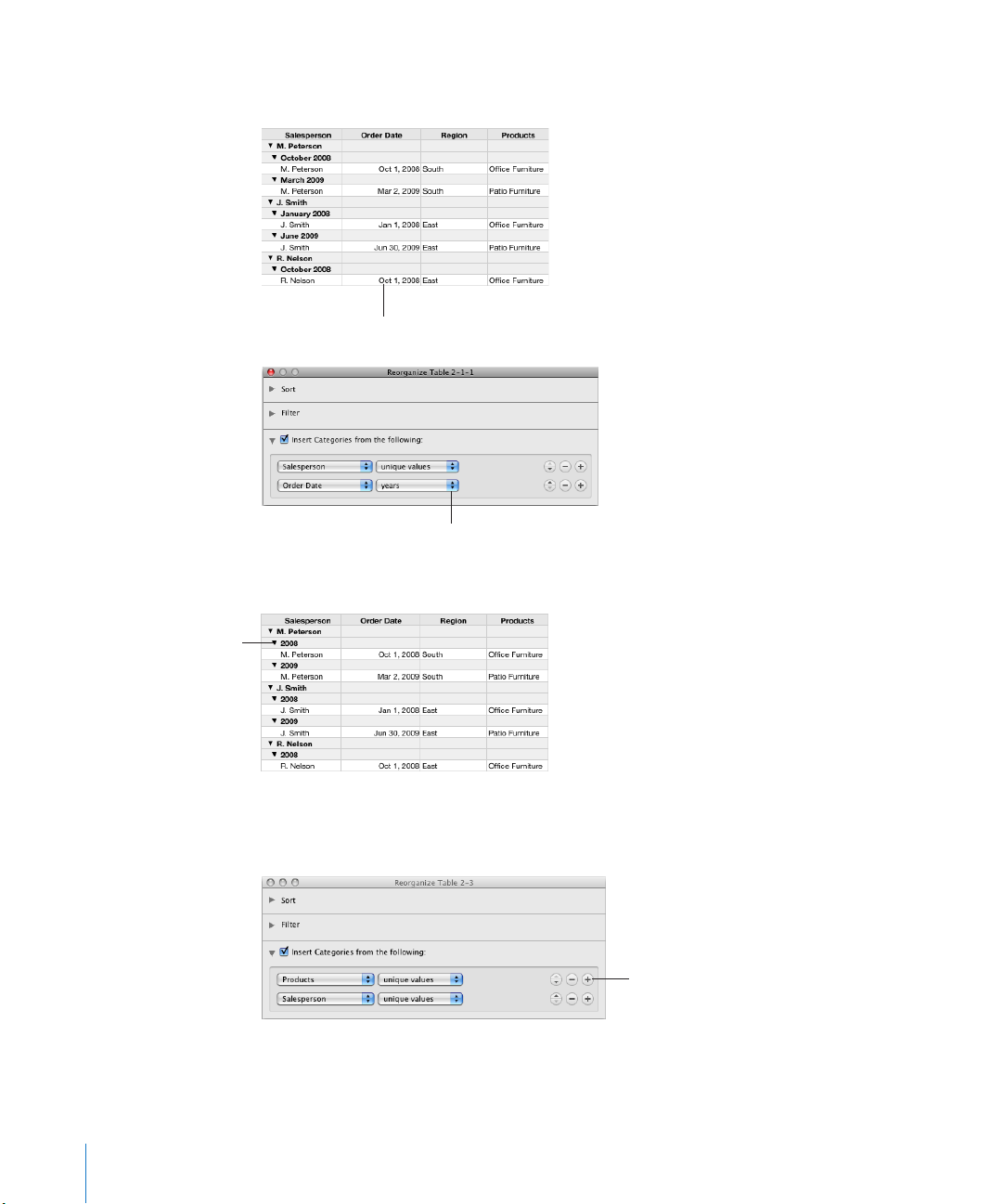
If the category value column contains dates, you can choose a date unit from the

Category column that contains dates

Choose a date unit.

Category rows

display years because

“years” was selected in the

Reorganize window.

Click to add subcategory.

second pop-up menu.

The date unit you select controls how the rows are categorized as well as how the

category is identied in the category row.

To create a subcategory, open the Reorganize window, and click the Add (+) button m adjacent to the category or subcategory below which you want the new subcategory. Then choose the column whose values you want to use for the subcategory.

70 Chapter 3 Using Tables

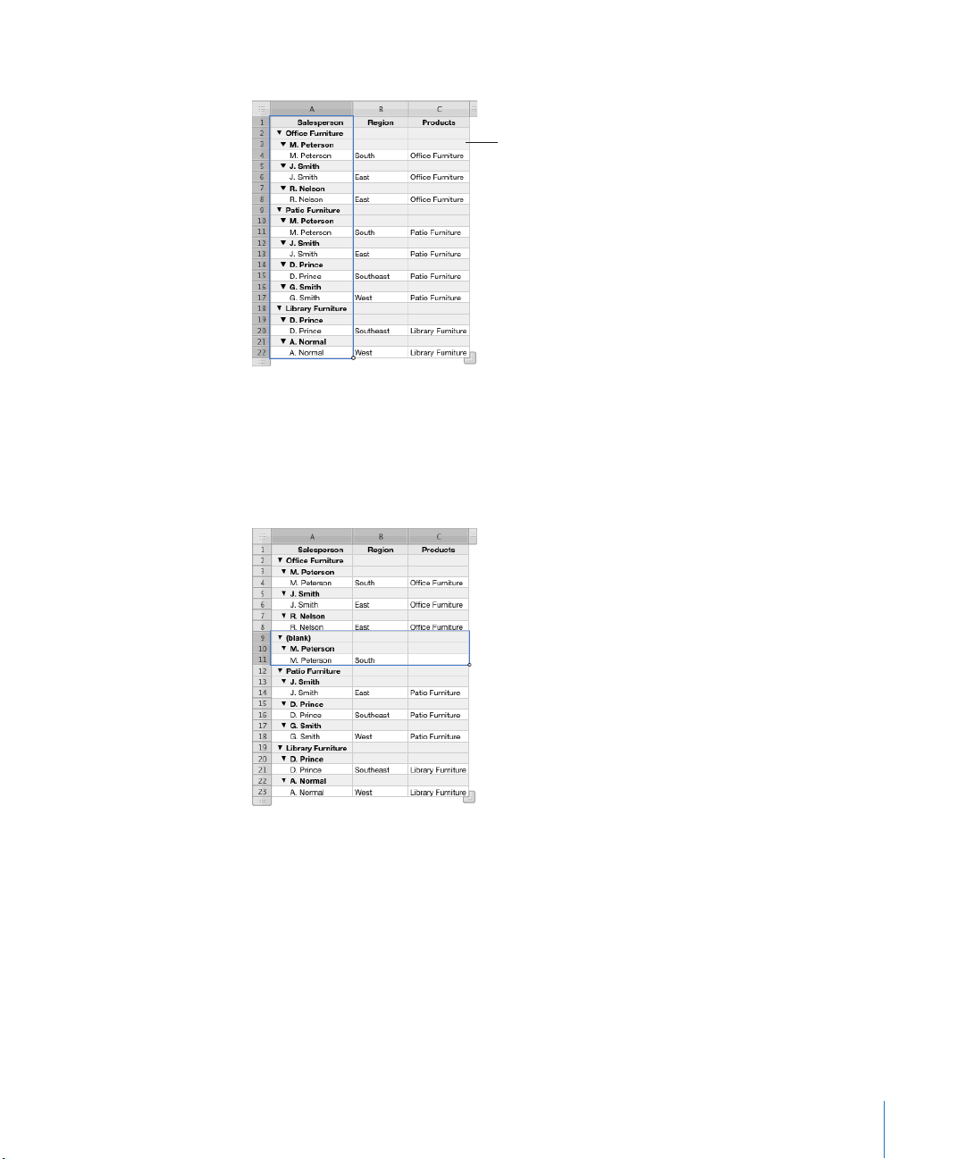
Each subcategory has its own category row in the table.

Subcategory row

To add a category or subcategory above or below an existing category or subcategory, m in the cell reference pop-up menu for the category or subcategory, choose Add Category Above or Add Category Below.

If you delete a value from a category value column, its row is placed into a category with blank values in the column.

If you delete all rows from a category, the category is removed from the table.

Chapter 3 Using Tables 71

Removing Table Categories and Subcategories

You can remove categories and subcategories temporarily, or you can discontinue using them altogether.

Here are ways to uncategorize rows:

To temporarily uncategorize all the rows in a table, click in the table and then click m Reorganize in the toolbar, or choose Show More Options from a reference tab’s pop-up menu to open the Reorganize window. Deselect “Insert Categories from the following.” To restore categorizing, select “Insert Categories from the following.”

You can also choose Table > Disable All Categories. To restore categories, choose Table > Enable All Categories.

To discontinue categorizing a table, in the Reorganize window click the Delete (–) m button adjacent to each category and subcategory.

You can also click the cell reference pop-up menu for a category row at the topmost level and choose Delete Categories.

To stop using a particular column as a category value column, in the Reorganize m window click the Delete (–) button adjacent to the column.

You can also choose Delete Categories from the column’s reference tab pop-up menu.

Managing Table Categories and Subcategories

Here are techniques for managing categories:

To move a row from one category to another, select the row and drag it into the m new category.

To move a category within a table, click the reference tab for its category row and drag the category to the new location.

To move a category up or down a level, click Reorganize in the toolbar, or choose m Show More Options from a reference tab’s pop-up menu to open the Reorganize window. Click the Move Up button or the Move Down button adjacent to a column.

You can also click the reference tab pop-up menu for a category row, and then choose Promote (to move a category to a higher level) or Demote (to move it to a lower level).

To format a category row, select one or more cells and then use the format bar or the m

Graphics inspector to modify background ll and text style. The changes are applied to

all cells in the current category row and all other category rows at the same level.

72 Chapter 3 Using Tables

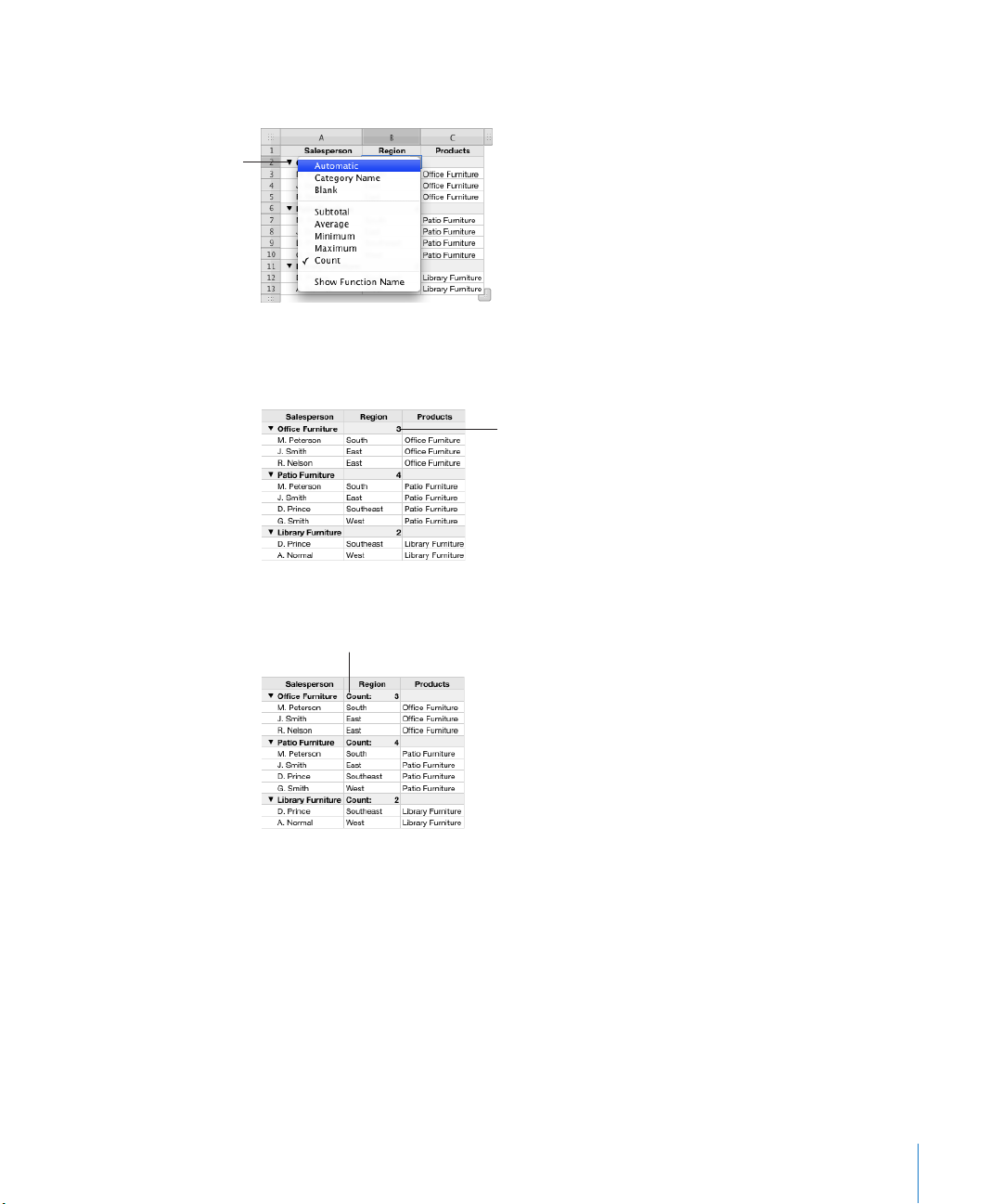
To display values automatically computed using cell values in a column of a category m

Click a disclosure

triangle to choose a

computation type.

Count of non-blank cells

Function name displayed

or subcategory, click a category row cell and then click the disclosure triangle.

Choose a numeric computation type (Subtotal, Average, and so on) to display the results of operations on numeric values (except date, time, or duration values); choose Count to display a count of nonblank cells.

To display the kind of calculation being shown, choose Show Function Name from the pop-up menu after choosing a computation type.

To remove the contents of a cell in a category row, choose Blank from the cell’s m pop-up menu.

To display the category name in the cell, choose Category Name instead.

To add a new row to a category or subcategory, choose Add Row Above or Add Row m Below from a row’s cell reference pop-up menu. When the new row is added, cells in the category value columns are assigned the values for the category or subcategory

Chapter 3 Using Tables 73

where the row was inserted.

To hide rows, select them and choose Hide Selected Rows from a row reference tab m pop-up menu.

Body rows in the selected range are hidden, but category rows reman visible.

To expand or collapse all category or subcategories of the same level, choose Expand m All or Collapse All from the cell reference pop-up menu of any row at the same level that you want to expand or collapse.

To expand or collapse all categories and subcategories of all levels, hold down the m Option key as you click the disclosure triangle near the left edge of any category row.

If one or more categories at the same level are collapsed, then Option-clicking will expand all categories.

If one of more categories at the same level are expanded, then Option-clicking will collapse all categories.

74 Chapter 3 Using Tables

Working with Table Cells

This chapter describes how to work with table cells and their content.

Putting Content into Table Cells

Use a variety of techniques to add content to table cells.

To learn how to Go to

Add, replace, copy, paste, and move table cell values

Format and align text in table cells and use nd-

and-replace and spell-checking features

Work with numeric table cell values “Working with Numbers in Table Cells” on

Use autolling to automatically repeat a cell value

in adjacent cells

“Adding and Editing Table Cell Values” on page 75

“Working with Text in Table Cells” on page 76

page 77

“Autolling Table Cells” on page 78

Adding and Editing Table Cell Values

You can add, change, and delete the content in cells.

Here are ways to add and edit values:

If the cell is empty, select it and then type a value. “ m Selecting a Table Cell” on page 52 describes how to select cells.

To replace specic content already in the cell, select the cell and then select what you m

want to replace by double-clicking; hold down the Shift key and select more content if you want to replace more. Type to replace the selected content.

To replace everything in the cell, select the cell and then begin typing. m

If “Return key moves to next cell” isn’t selected in the Table inspector, you can also select the cell and then press Return or Enter, which selects everything in the cell, and then start typing.

To insert content within existing content, select the cell, click to set the insertion point, m

Align text to the left, center, right; justify text; or align text to the left and numbers to the right.

Align text to the top, middle, or bottom of cells.

and begin typing.

To undo changes made to a table cell since selecting the cell, press Esc. m

To delete the content of table cells, rows, or columns, select the cells, rows, or columns m and then press the Delete key or choose Edit > Delete.

To delete the contents, background ll, and any style settings, choose Edit > Clear All.

The default style is applied to the selection.

To copy, paste, and move cell values, see the instructions in “ m Copying and Moving Cells” on page 85.

To add formulas and functions to cells, see the instructions in “ m Creating Your Own Formulas” on page 11 8 .

Working with Text in Table Cells

You can control the format and alignment of text in table cells, and you can use

nd-and-replace and spell-checking features.

When you type text into a cell, Numbers displays text that might be used to complete the cell content based on similar text elsewhere in the table. You can use the suggested text if it’s appropriate, or you can keep typing to override suggestions. To disable auto-suggestions, deselect “Show auto-completion list in table columns” in the General pane of Numbers preferences.

Here are techniques for working with text in table cells:

To insert a line break, press Option-Return. m

To insert a paragraph break, if “Return key moves to next cell” below Table Options in m the Table inspector isn’t selected, press Return. Otherwise, press Option-Return.

You can also click in the formula bar and click the line break button in the format bar.

To insert a tab in a table, press Option-Tab. m

You can also click in the formula bar and click the tab button in the format bar.

To adjust text alignment, use the alignment buttons in the format bar. m

The Text inspector gives you additional text formatting options (click Inspector in the toolbar and click the Text inspector button).

76 Chapter 4 Working with Table Cells

See “Setting Text Alignment, Spacing, and Color” on page 170 for more information.

To control font attributes, use the text formatting buttons in the format bar. m

Choose a font.

Choose a typeface.

Choose the font size.

Choose the text color.

You can also use the Fonts window (click Fonts in the toolbar).

See “Formatting Text Size and Appearance” on page 16 3 for additional information.

To check spelling, follow the instructions in “ m Checking for Misspelled Words” on page 187.

To nd and optionally replace text in cells, follow the instructions in “ m Searching for and

Replacing Text” on page 18 9.

To avoid having Numbers interpret what you type as a number, use the text format. m See “Using the Text Format in Table Cells” on page 96 for details.

Note: Text strings are ignored in functions that use values to perform calculations.

Working with Numbers in Table Cells

Some table operations, such as formulas and functions that perform mathematical operations, depend on cells containing numeric values.

Here are techniques for working with numbers in table cells:

In a numeric cell use only numbers (0 through 9) or one of the following characters: m plus sign (+), minus sign (–), left or right parenthesis ( ), forward slash (/), currency symbol (for example, $), percent sign (%), period (.), capital E, or lowercase e.

You can type some characters (such as %) into a cell, or you can use a cell format, as m “Formatting Table Cell Values for Display” on page 86 describes.

To specify a negative number, precede it with the minus sign (–). m

When you put a number in a table cell that’s too large to display, Numbers converts the number:

When a decimal number doesn’t t in a cell, the number is rounded. For example, Â

1.77777777777777777777 becomes 1.77777777777778.

When a whole number doesn’t t in a cell, the number is displayed using scientic Â

notation. For example, 77777777777777777777 becomes 7.777778E+19.

Scientic notation displays numbers using an exponent raised by the power of 10.

The exponent is displayed following the E.

If the converted number still doesn’t t, it’s clipped. See “Displaying Content Too Large

for Its Table Cell” on page 79 for suggestions.

Chapter 4 Working with Table Cells 77

Instructions for using formulas and functions in table cells are in “Creating Your Own Formulas” on page 11 8 .

Autolling Table Cells

With autolling you can use the content in one or more cells to automatically add

values to adjacent cells.

Here are ways to autoll table cells:

To paste the content and ll of a cell into adjacent cells, select the cell and then drag m

the Fill handle (a small circle in the cell’s lower-right corner) over the cells into which you want to paste.

Any data, cell format, formula, or ll associated with the selected cell is pasted, but comments aren’t pasted. If any target cell contains data, autolling overwrites that

data with the value you’re repeating.

To paste the content and ll of a cell into one or more cells in the same row or column, m

select two or more adjacent cells and choose one of the following:

Insert > Fill > Fill Right: Assigns selected cells the value in the leftmost selected cell.

Insert > Fill > Fill Left: Assigns selected cells the value in the rightmost selected cell.

Insert > Fill > Fill Up: Assigns selected cells the value in the bottommost selected cell.

Insert > Fill > Fill Down: Assigns selected cells the value in the topmost selected cell.

Any data, cell format, formula, or ll associated with the selected cell is pasted, but comments aren’t pasted. If any target cell contains data, autolling overwrites that

data with the value you’re repeating.

You can also add values to cells based on value patterns. For example, if a cell contains m a day of the week or a month, you can select the cell and then drag to the right or down to add the next day of the week or month to the adjacent cell.

To create new values based on numeric patterns, select two or more cells before dragging. For example, if two selected cells contain 1 and 2, the values 3 and 4 are added when you drag through the adjacent two cells. And if two selected cells contain 1 and 4, the values 7 and 10 are added when you drag through the adjacent two cells (values are incremented by 3).

Autolling doesn’t set up an ongoing relationship among cells in the group. After autolling, you can change the cells independently of each other.

78 Chapter 4 Working with Table Cells

Displaying Content Too Large for Its Table Cell

The clipping indicator

When a cell is too small to display all its content, here is what happens:

If the content is a number or date, a clipping indicator appears. Â

For other types of values, no clipping indicator appears. You can only see content Â that’s visible within the boundaries of its cell.

Here are ways to handle content too large for a cell:

To let a value in a cell spill into adjacent cells, deselect Wrap in the format bar or m deselect “Wrap Text in Cell” in the Cells inspector. Numbers and dates clip instead of spill, even with wrap deactivated.

If the adjacent cells are empty, they display spilled content. But if they contain data,

content that doesn’t t isn’t displayed, and the clipping indicator appears.

To make content wrap instead of spill, select Wrap in the format bar or “Wrap Text in Cell” in the Cells inspector.

If cell values aren’t visible because columns are too narrow, you can use the Fit button m next to the Column Width controls in the Table inspector to make values visible. Select a cell, one or more columns, or the table, and then click the Fit button.

You can also resize a column by dragging the right border of its reference tab to the right, or by using the Column Width controls in the Table inspector.

If cell values aren’t visible because rows are too narrow, you can use the Fit button m next to the Row Height controls in the Table inspector to make values visible. Select a cell, one or more rows, or the table, and then click the Fit button. As row content is added or removed, row height automatically changes to match content height.

You can also resize a row by clicking the bottom border of its reference tab and dragging down, or by using the Row Height controls in the Table inspector.

You can also resize columns and rows to accommodate content by using the m reference tabs.

To increase the height of a row to accommodate its largest content, double-click the lower border of the row’s reference tab. Column width does not adjust automatically when you make content changes.

To increase the width of a column to accommodate its largest content, double-click the right border of the column’s reference tab.

Chapter 4 Working with Table Cells 79

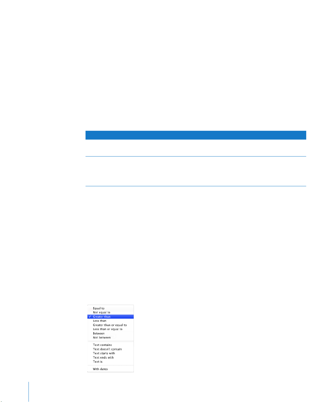
Using Conditional Formatting to Monitor Table Cell Values

Conditional formatting changes a cell’s appearance when the cell contains a particular value, referred to as a test value.

To apply conditional formatting, you select one or more cells and then dene one or more rules. The rules specify which visual eects to associate with cells when they

contain the test value.

For example, you can dene a rule that lls a cell with blue when it contains 0, a rule that displays the cell’s value as boldface black if it’s greater than 0, and a rule that lls

the cell with red if its value is less than 0.

Rules applied to multiple cells trigger conditional formatting in any of the cells that contain the test value.

To learn how to Go to

Create rules “Dening Conditional Formatting Rules” on

page 80

Remove all conditional formatting from cells,

change rules, nd cells that use the same

conditional formatting, copy/paste conditional formatting between tables

Dening Conditional Formatting Rules

A conditional formatting rule is used to detect when cells contain a test value, which

can be either a specic value that you supply or a value that matches a value currently in a specic table cell. The rule species the formatting to apply to the cells when they

contain the test value.

“Changing and Managing Your Conditional Formatting” on page 82

To dene rules:

1 Select one or more cells.

2 Click Inspector in the toolbar, click the Cells inspector button, and then click

“Show rules.”

You can also choose Format > Show Conditional Format Rules.

3 Choose an option from the “Choose a rule” pop-up menu.

80 Chapter 4 Working with Table Cells

The options in the top section of the menu apply tests to numeric values. Options in

Click to select a table cell.

the middle section are for text values. The “With dates” option is for dates.

4 To specify a specic test value, type it into the value eld, to the right of the

pop-up menu.

You can also use the value in a table cell as a test value. To do so, click the small blue

circle in the value eld.

The cell reference eld appears.

Specify a cell reference by clicking a table cell. You can also type a cell reference and press Return; see “Referring to Cells in Formulas” on page 12 3 for information about writing cell references.

The Between rule requires that you specify two test values. The formatting is applied if either of the numbers or any number in between them appears in the cell or cells.

For the “With dates” rule, before specifying a test value choose options from the

pop-up menus on both sides of the test value eld.

5 To specify formatting to apply when cells contain the test value, click Edit.

Text color well: Click it to select a color to apply to cell values.

Font style buttons: Click B to show cell values in boldface, click I to show them in

italics, click U to underline cell values, or click T to apply the strikethrough style.

Chapter 4 Working with Table Cells 81

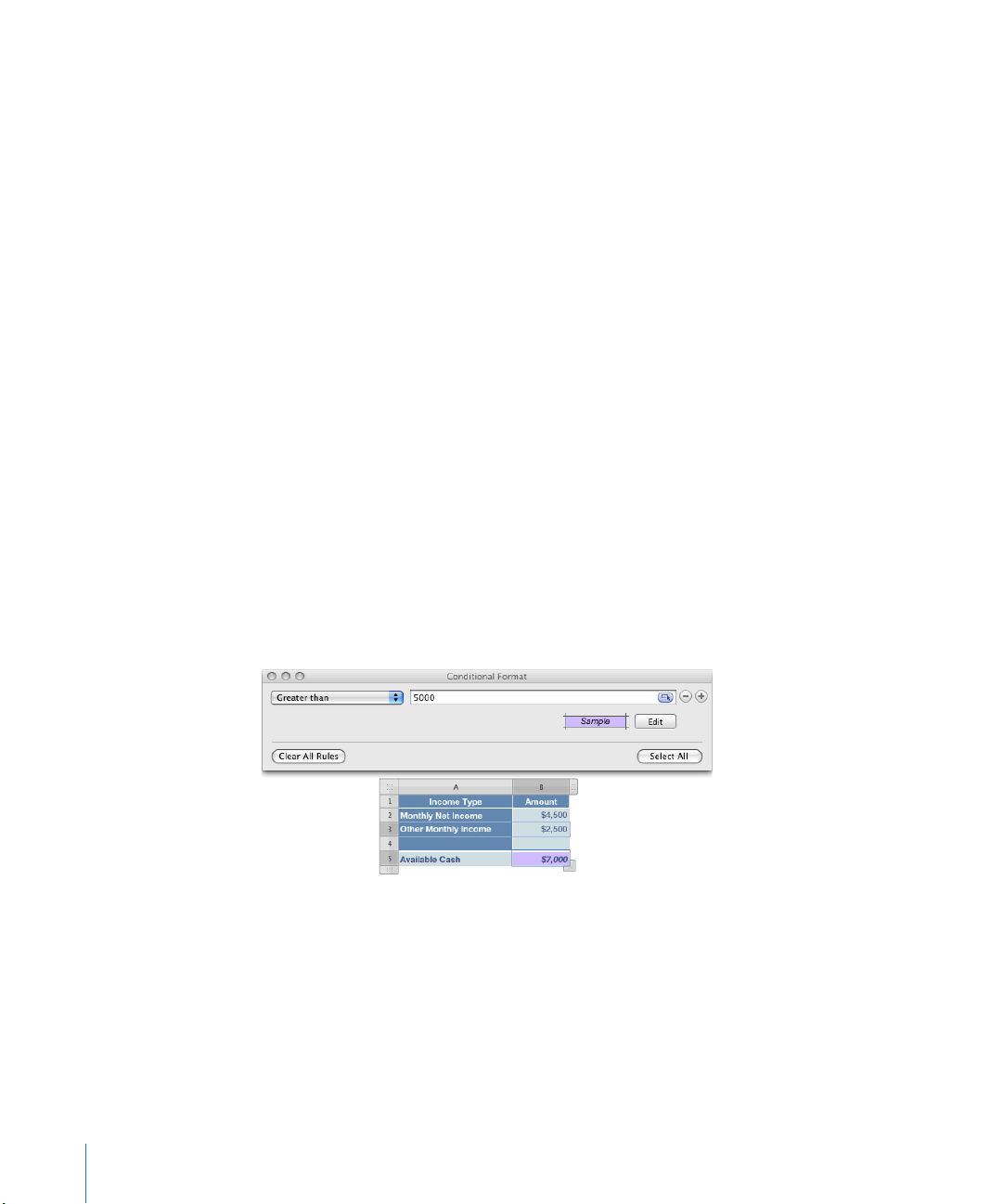
Fill color well: Click it to select a cell ll color.

As you click, the Sample box displays the eect of your selections. When you’re satised with the eect, click Done.

6 To add another rule, click the Add button (+) and repeat steps 3 through 5.

If more than one rule is dened for a cell, and the cell’s value satises the conditions of

multiple rules:

The text color applied is the color associated with the topmost rule with a text color Â

specied.

The font style applied is the font style associated with the topmost rule that has a Â

font style specied.

The ll color applied is the ll color associated with the topmost rule that has a ll Â color specied.

After the text color you specify has been applied to a cell value, if you type new text into the cell after placing an insertion point and changing the text color in the format bar or the Text inspector, the new text appears in the new text color, but the existing text retains the color you set in the rule.

Changing and Managing Your Conditional Formatting

Here are techniques you can use:

To nd all the cells in a table that have the same conditional formatting rules as m a particular cell, select the cell, click “Show rules” in the Cells inspector, and then click “Select All.” Cells with matching rules are selected in the table.

To remove all conditional formatting associated with cells in a table, select the cells, m click “Show rules” in the Cells inspector, and then click Clear All Rules.

To apply the same conditional formatting rules to cells in dierent tables, select m a cell whose rules you want to reuse, choose Edit > Copy, select one or more cells

in a dierent table, and then choose Edit > Paste.

To add or remove a conditional formatting rule, click the Add (+) or Delete (–) button m in the Conditional Format window.

82 Chapter 4 Working with Table Cells

To change a rule, redene its pop-up menu options, test values, or formatting. Here are m some techniques for working with test values that are specied as cell references:

To delete a test value that’s a cell reference, click in the test value eld and press Delete.

To replace a cell reference with a dierent one, click in the test value eld and click a dierent cell in the same table or a dierent table.

To replace a textual test value with a cell reference, click in the test value eld, click the

small blue circle, and then click a table cell.

Adding Images or Color to Table Cells

You can add graphics or color to individual table cells or to an entire table.

To add an image or color to a table cell:

1 Select the cell.

2 Click Inspector in the toolbar, and then click the Table inspector.

3 To add an image, choose Image Fill from the Cell Background pop-up menu. See

“Filling an Object with an Image” on page 225 for instructions.

4 To add background color, choose Color Fill or Gradient Fill from the Cell Background

pop-up menu. See “Filling an Object with a Solid Color” on page 223 and “Filling an Object with Blended Colors (Gradients)” for more information.

Merging Table Cells

Merging table cells combines adjacent cells into one, eliminating the borders so that they behave as a single cell.

To merge table cells:

1 Select a group of two or more adjacent table cells. The group of cells you choose must

form a rectangle, and they must be all body cells, all header cells, or all footer cells.

2 Choose Table > Merge Cells.

You can also click the Merge button in the Table inspector.

To unmerge cells, select a cell created by merging, and then deselect Merge Cells in the Table menu or click the Unmerge button in the Table inspector.

Here is what happens to cell content during a merger:

Merging horizontally contiguous cells containing only text or a mixture of text, Â numbers, formatted values, and formulas joins the content from all the original cells as text separated by tabs.

Merging vertically contiguous cells containing only text or a mixture of text, numbers, formatted values, and formulas joins the content from all the cells as text separated by carriage returns.

Chapter 4 Working with Table Cells 83

When you merge column cells, the cell background takes on the image or color that Â

Click to choose a stroke color.

Click to choose a stroke style.

Click to choose a line thickness.

was in the topmost cell.

When you merge row cells, the cell background takes on the image or color that was in the leftmost cell.

When a cell containing text, a number, a formula, or a cell format is merged with an Â empty cell, the new cell retains the content of the non-empty cell.

When a cell containing a number format is merged with an empty cell, the new cell Â retains the number format.

Rows and columns that contain merged cells can’t be hidden.

Splitting Table Cells

Splitting cells divides each selected cell into two equal parts, horizontally (rows) or vertically (columns). Both of the new cells have identical background colors or images. Any text that was in the original cell remains in the topmost or leftmost cell.

To split cells horizontally or vertically:

1 Select a table cell or cells. To split an entire row or column, select all the cells in the row

or column.

2 To split cells into rows, choose Table > “Split into Rows.” To split cells into columns,

choose Table > “Split into Columns.”

You can also click the Split button in the Table inspector.

3 To create smaller and smaller units, repeat steps 1 and 2 for the split cells.

To rejoin split cells, merge them, as “Merging Table Cells” on page 83 describes.

Formatting Table Cell Borders

You can change the line thickness and color of table cell borders. Or you can hide the border of any cell.

To format table cell borders:

1 Select the cell border segments you want to format. See “Selecting Table Cell

Borders” on page 54 for instructions.

2 Use the controls in the format bar or in the Table inspector.

Stroke pop-up menu: Lets you choose a stroke style. Choose None to hide borders.

Line thickness: Controls the thickness of the stroke.

84 Chapter 4 Working with Table Cells

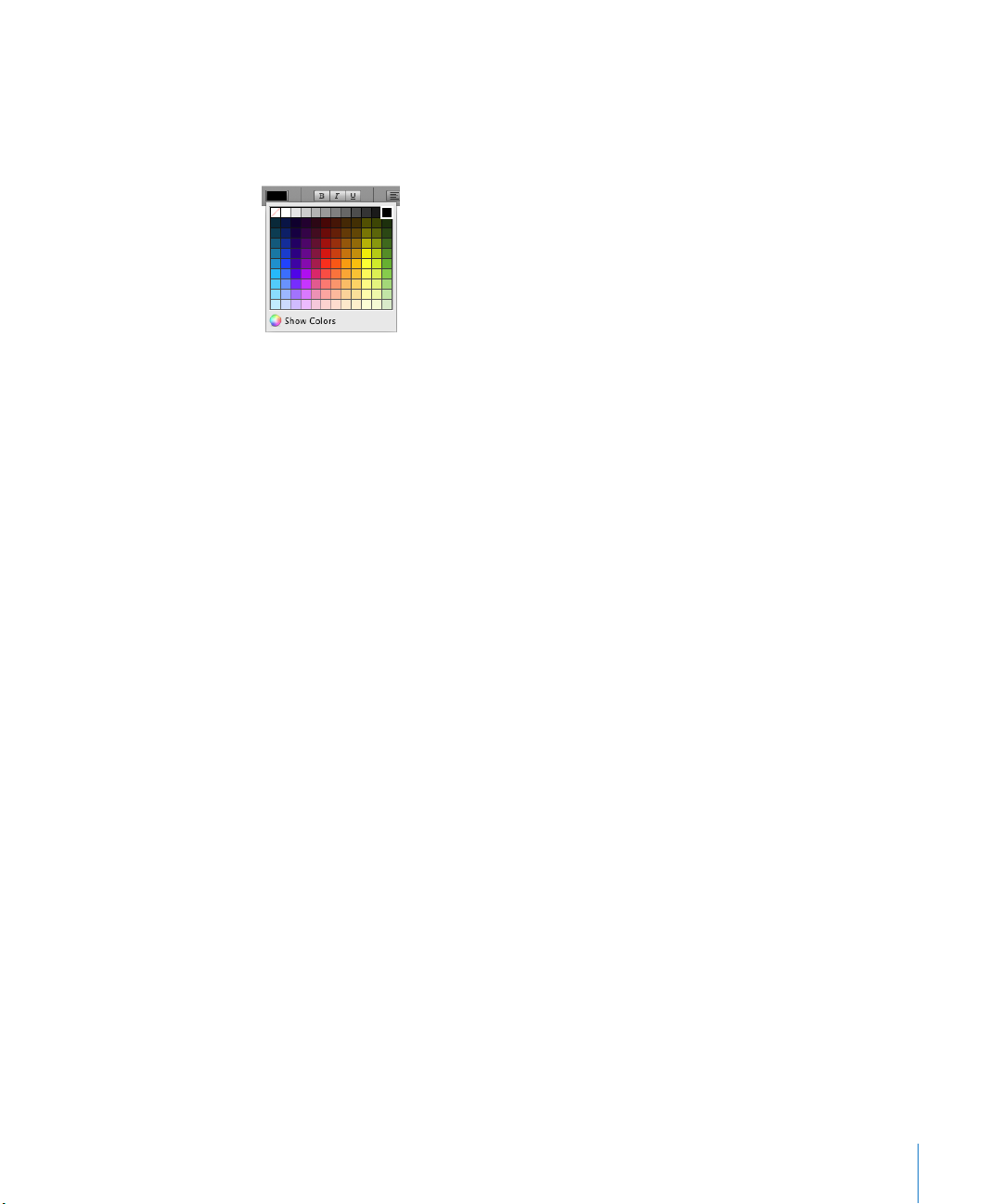
Color well: Lets you choose a stroke color.

When you click the color well in the format bar, a color matrix appears. Select a color by clicking it in the matrix, or click Show Colors to open the Colors window for additional color options.

When you click the color well in the Table inspector, the Colors window opens. “The Colors Window” on page 24 provides instructions for using this tool.

Copying and Moving Cells

Here are ways to copy and move cells:

To move cells within a table, to another table, or to the canvas, select a cell or several m adjacent cells, and then when the pointer changes to a white cross drag the selection until any destination cells are selected. Values in the destination cells are replaced, and the values in the original location are removed.

To copy cells within a table, to another table, or to the canvas, drag selected cells while m holding down the Option key. Any values in the destination cells are replaced, and the values in the original location are retained.

You can also copy cells by selecting them, choosing Edit > Copy, selecting destination cells, and then choosing Edit > Paste.

You can also paste a cell’s content into multiple cells, which don’t have to be adjacent to the copied cell or to each other. After copying a cell, select the destination cells and choose Edit > Paste. The cell’s contents are copied to all the destination cells, in the same or another table, replacing any existing content.

To insert copied cells without overwriting destination cells, choose Insert > Copied m Columns or choose Insert > Copied Rows after selecting destination cells.

Copied Columns: Adds new columns to accommodate copied cells.

Copied Rows: Adds new rows to accommodate copied cells.

When you paste a cell’s contents into a dierent cell, any comment associated with the

pasted content is also pasted.

If you delete the contents of a cell, any comment associated with the cell is removed.

Chapter 4 Working with Table Cells 85

See “Rearranging Rows and Columns” on page 58 to learn how to copy and move rows and columns using the reference tabs.

See “Copying or Moving Formulas and Their Computed Values” on page 12 8 to learn about techniques for duplicating or moving a cell that contains a formula.

Adding Comments to Table Cells

Use comments to record information about table cells.

Here are ways to work with comments:

To add a comment to a cell, select the cell and click Comment in the toolbar, or choose m Insert > Comment. Type in the comment box.

To move a comment, drag it. m

To hide all comments, choose View > Hide Comments. A yellow marker appears in any m table cell containing a comment.

To hide one comment, click the Minimize (–) button in the upper left of the comment box, or click the comment marker. A hidden comment can be temporarily displayed by placing the pointer over the marker.

To show all comments, choose View > Show Comments. m

To show a hidden comment, click its marker.

To delete a comment, click the X in the upper right of the comment box. m

To include comments when you print, show any comments you want to print, m and then choose File > Print.

Formatting Table Cell Values for Display

You can apply a format to a cell to display its value in a particular way. For example, you can apply the currency format to cells that hold monetary values so that a currency symbol (such as $, £, or ¥) appears in front of numbers in the cells.

When you use a cell format, you are setting only the display characteristics of a value. When the value is used in formulas, the actual value is used, not the formatted value. The only exception is when there are too many numbers following a decimal point, in which case the number is rounded.

Here are ways to work with cell formats:

You apply cell formats by selecting one or more cells and then using the format bar or m the Cell Format pop-up menu in the Cells inspector to select the format.

To add a value to an empty cell that has a format, select the cell and enter a value. m The format is applied when you leave the cell.

86 Chapter 4 Working with Table Cells

If you delete a value from a cell with a format, the cell’s format isn’t deleted. To m delete the format, apply the automatic format. To delete the value and format, choose Edit > Clear All.

After you dene a cell format, you can associate the format with multiple cells by using m autolling. See “Autolling Table Cells” on page 78 for instructions.

To see the unformatted content in a cell to which formatting has been applied, select m the cell and view the actual value in the formula bar.

Use this cell format When you want to Learn more here

automatic Automatically format content

based on the characters it contains

number Format the display of a

number’s decimal places, thousands separator, and negative values

currency Format the display of monetary

values

percentage Display numeric values followed

by the % symbol

date and time Format how date and time

values are displayed

duration Format the display of week,

day, hour, minute, second, and microsecond values

fraction Format the display of any part

of a value smaller than 1

numeral system Format the display of numbers

using the conventions of a particular numeral system (such as decimal or binary)

scientic Format the display of numbers

using an exponent raised by the power of 10

text Display cell content exactly as

you type it

cell controls (checkboxes, slider, stepper, or pop-up menu)

custom Dene your own cell format “Using Your Own Formats for

Control the specic values a cell

can contain

“Using the Automatic Format in Table Cells” on page 88

“Using the Number Format in Table Cells” on page 89

“Using the Currency Format in Table Cells” on page 90

“Using the Percentage Format in Table Cells” on page 91

“Using the Date and Time Format in Table Cells” on page 92

“Using the Duration Format in Table Cells” on page 93

“Using the Fraction Format in Table Cells” on page 93

“Using the Numeral System Format in Table Cells” on page 94

“Using the Scientic Format in Table Cells” on page 95

“Using the Text Format in Table Cells” on page 96

“Using a Checkbox, Slider, Stepper, or Pop-Up Menu in Table Cells” on page 96

Displaying Values in Table Cells” on page 98

Chapter 4 Working with Table Cells 87

Using the Automatic Format in Table Cells

When you add a new cell, its content is displayed using the automatic format.

This content in a cell assigned the automatic format

A number Decimal places and commas are preserved as

A currency value The displayed value shows 0 decimal places if it’s

A date value The value is formatted using the date format

A Boolean value The values “true” and “false” are converted to

A percentage value A number followed by the % sign is displayed as

A scientic value The display format rounds the value to 2 decimal

Is formatted like this for display

entered.

For example, 1,000,000.008 displays as 1,000,000.008.

an integer ($50); otherwise it shows 2 decimal places. If there are more than 2 decimal places, rounding is applied.

For example, $1,000.0075 displays as $1,000.01.

specied in System Preferences (search for “date

format” in System Preferences) and is treated as a date value in formulas. To view the date formats in Numbers, open the Cells inspector and choose “Date and Time” from the Cell Format pop-up menu. Then select the Date pop-up menu.

A 2-digit year value greater than 50 is displayed

using the prex 19; otherwise the prex 20 is

used.

For example, 1/1 displays as Jan 1, 2008, and Jan 05 displays as Jan 5, 2008.

“TRUE” and “FALSE.” These cells can be used in

Boolean operations in formulas.

entered, and in formulas the value is treated as a percentage value. A space before the % sign is not required.

For example, you can type 5% or 5 %.

places.

For example, 1.777E3 is displayed as 1.78+E3.

88 Chapter 4 Working with Table Cells

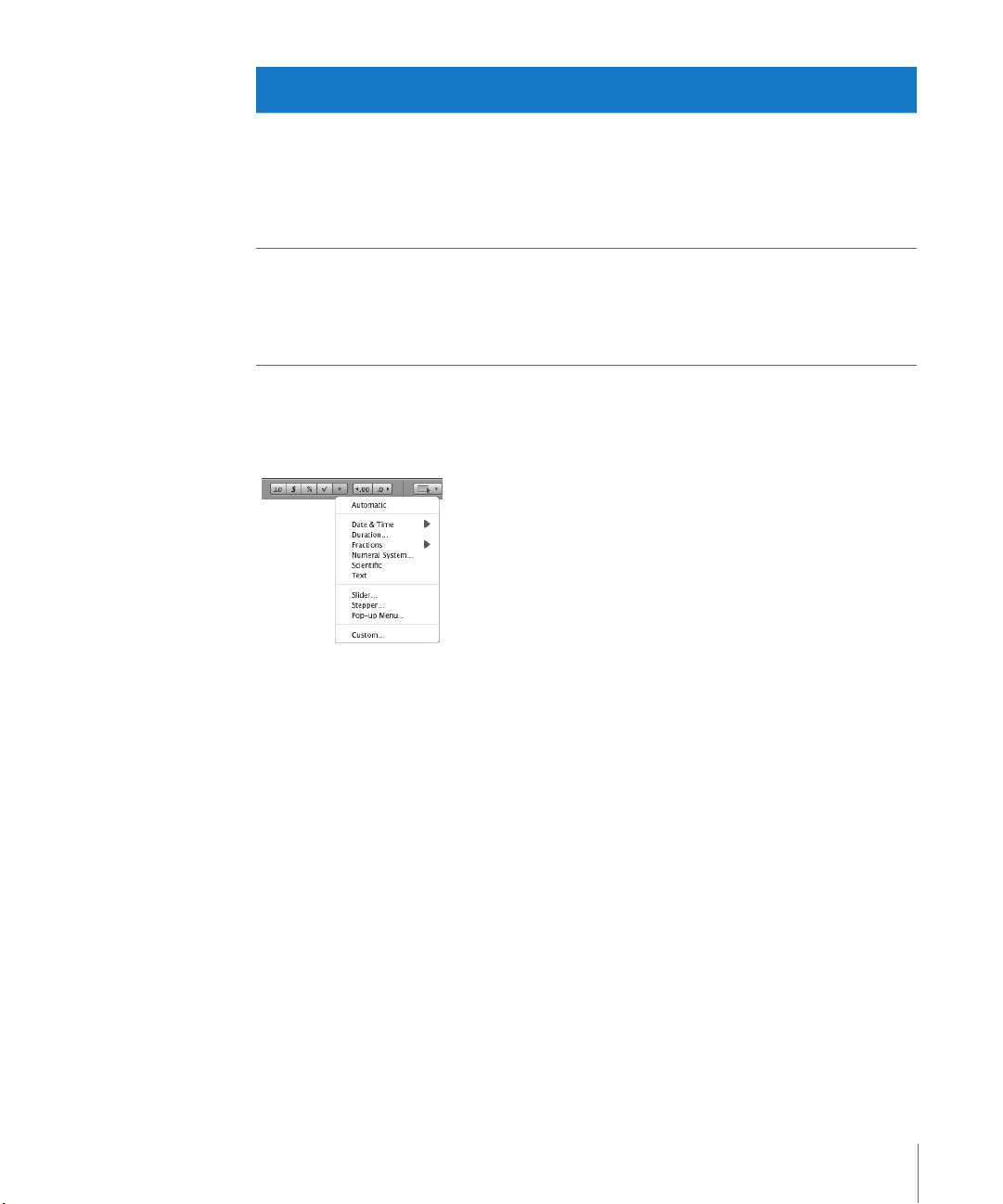
This content in a cell assigned the automatic format

A duration value A number accompanied by a duration sux

A fraction value The value is formatted like a date if it matches

Is formatted like this for display

(w or weeks, d or days, h or hours, m or minutes, s or seconds, ms or milliseconds) is treated as a

duration value in formulas. The sux is displayed

in its abbreviated form.

For example, 2 weeks is displayed as 2w.

one of the formats available for date values. Otherwise, the “Up to three digits” accuracy is used for display.

For example, 1/1 displays as Jan 1, 2008.

If a dierent format has been applied to a cell, you can change its format to automatic

by selecting the cell and choosing Automatic from the Cell Formats pop-up menu in the format bar.

You can also use the Cells inspector.

To apply the automatic format using the Cells inspector:

1 Select the cell or cells.

2 Click Inspector in the toolbar, and then click the Cells inspector button.

3 Choose Automatic from the Cell Format pop-up menu.

Using the Number Format in Table Cells

Use the number format to format the display of a number’s decimal places, thousands separator, and negative values.

Chapter 4 Working with Table Cells 89

To dene a number format that displays two decimal places, a thousands separator,

Number Format button

Increase Decimal

Places button

Decrease Decimal Places button

Currency Format button

and negative numbers with the negative symbol, select one or more cells and then click the Number Format button in the format bar. Use the Decrease Decimal Places and Increase Decimal Places buttons located nearby to change the number of decimal places.

For more control over the number format, use the Cells inspector.

To dene a number format using the Cells inspector:

1 Select the cell or cells.

2 Click Inspector in the toolbar, and then click the Cells inspector button.

3 Choose Number from the Cell Format pop-up menu.

4 To specify how many decimal places to display, use the Decimals eld.

If a value contains more decimal places than you specify, the decimal value displayed is rounded, not truncated. For example, if a cell is formatted to display two decimal places, the value 3.456 is displayed as 3.46, not 3.45.

5 To specify how to display negative values, choose an option from the pop-up menu

adjacent to the Decimals eld.

6 To specify whether to use a thousands separator, select or deselect Thousands

Separator.

Using the Currency Format in Table Cells

Use the currency format to format the display of monetary values.

To dene a currency format that displays two decimal places, a thousands separator,

and negative numbers with the negative symbol, select one or more cells and then click the Currency Format button in the format bar. Use the Decrease Decimal Places and Increase Decimal Places buttons located nearby to change the number of decimal places.

For more control over the currency format, use the Cells inspector.

90 Chapter 4 Working with Table Cells

To dene a currency format using the Cells inspector:

Increase Decimal

Places button

Decrease Decimal Places button

Percentage Format button

1 Select the cell or cells.

2 Click Inspector in the toolbar, and then click the Cells inspector button.

3 Choose Currency from the Cell Format pop-up menu.

4 To specify a currency symbol, choose an option from the Symbol pop-up menu.

You can maximize the number of options in the Symbol pop-up menu by choosing Numbers > Preferences and then selecting “Show complete list of currencies in Cell inspector” in the General pane.

5 To specify how many decimal places to display, use the Decimals eld. If a value

contains more decimal places than you specify, the decimal value displayed is rounded, not truncated. For example, if a cell is formatted to display two decimal places, the value 3.456 is displayed as 3.46, not 3.45.

6 To specify how to display negative values, choose an option from the pop-up menu

adjacent to the Decimals eld.

7 To specify whether to use a thousands separator, select or deselect Thousands

Separator.

8 To display the currency symbol at the edge of the cell, select Accounting Style.

Using the Percentage Format in Table Cells

Use the percentage format to display numeric values followed by the percent symbol (%).

If the value is used in a formula, its decimal number version is used. For example, a value that displays as 3.00% is used as 0.03 in a formula.

If you type 3% in a cell formatted using the automatic format and then apply the percentage format to the cell, the value displayed is 3%. However, if you type 3 in a cell formatted using the automatic format and then apply the percentage format to the cell, the value displayed is 300%.

To dene a percentage format that displays two decimal places, a thousands separator,

and negative numbers with the negative symbol, select one or more cells and then click the Percentage Format button in the format bar. Use the Decrease Decimal Places and Increase Decimal Places buttons located nearby to change the number of decimal places.

Chapter 4 Working with Table Cells 91

For more control over the percentage format, use the Cells inspector.

Cell formats button

Choose More to apply the template’s default date/time format and open the Cells inspector.

To dene a percentage format using the Cells inspector:

1 Select the cell or cells.

2 Click Inspector in the toolbar, and then click the Cells inspector button.

3 Choose Percentage from the Cell Format pop-up menu.

4 To specify how many decimal places to display, use the Decimals eld.

5 To specify how to display negative values, choose an entry from the pop-up menu

adjacent to the Decimals eld.

6 To specify whether to use a thousands separator, select or deselect Thousands

Separator.

If a cell you’re formatting already contains a value, the value is assumed to be a decimal value, and it’s converted into a percentage. For example, 3 becomes 300%.

Using the Date and Time Format in Table Cells

Use the date and time format to display date and/or time values.

To dene a date and time format, select one or more cells, click the Cell Formats

button in the format bar, choose Date & Time from the pop-up menu, and then choose an option from the submenu.

For more control over the date and time format, use the Cells inspector.

To dene a date and time format using the Cells inspector:

1 Select the cell or cells.

2 Click Inspector in the toolbar, and then click the Cells inspector button.

92 Chapter 4 Working with Table Cells

3 Choose “Date and Time” from the Cell Format pop-up menu.

4 To specify how you want a date formatted, choose a format from the Date

pop-up menu.

5 To specify how you want a time value formatted, choose a format from the Time

pop-up menu.

Using the Duration Format in Table Cells

Use the duration format for values that describe time increments, such as weeks, days, hours, minutes, seconds, or milliseconds.

To dene a duration format, select one or more cells, choose Duration from the Cell Formats pop-up menu in the format bar, and use the Cells inspector to specify the format.

To dene a duration format for selected cells using the Cells inspector:

1 Select the cell or cells.

2 If the Cells inspector isn’t already open, click Inspector in the toolbar and then click the

Cells inspector button.

3 Choose Duration from the Cell Format pop-up menu.

4 Use the Units control to select the units you want to display for a duration value.

By default, hours, minutes, and seconds (h, m, and s) are displayed.

To choose a single unit, drag the left or right end of the slider toward the center until it can get no shorter. Then click in the center of the slider and drag it over the unit you want to use.

To choose more than one unit, resize and drag the slider until it’s over the units you want to use.

5 From the Format pop-up menu, choose a display format.

Using the Fraction Format in Table Cells

Use the fraction format to control the display of any part of a value smaller than 1. For example, 27.5 displays as 27 1/2 when the format is Halves and as 27 4/8 when the format is Eighths.

Chapter 4 Working with Table Cells 93

To dene a fractions format, select one or more cells, choose Fractions from the Cell

Cell Formats button

Formats pop-up menu in the format bar, and then choose a format from the submenu.

You can also use the Cells inspector.

To dene a fraction format for selected cells using the Cells inspector:

1 Select the cell or cells.

2 Click Inspector in the toolbar, and then click the Cells inspector button.

3 Choose Fractions from the Cell Formats pop-up menu.

4 Choose a display format from the Accuracy pop-up menu.

Using the Numeral System Format in Table Cells

Use the numeral system format to represent numbers using the conventions of numeral systems from base 2 to base 36. When you use the Base 2, 8, or 16 format, you can display negative values by preceding them with a minus sign or in two’s complement notation; negative values in all other bases are displayed using the minus sign.

In this numeral system 100 displays like this –100 displays like this

Base 2 1100100 –1100100 10011100

Base 8 144 –144 634

Base 10 100 –100 –100

Base 16 64 –64 9C

94 Chapter 4 Working with Table Cells

if Minus Sign is used

–100 displays like this

if Two’s-Complement

is used

To dene a numeral system format, select one or more cells, choose Numeral System

from the Cell Formats pop-up menu in the format bar, and then use the Cells inspector to specify the format.

To dene a numeral system format for selected cells using the Cells inspector:

1 Select the cell or cells.

2 If the Cells inspector isn’t already open, click Inspector in the toolbar and then click the

Cells inspector button.

3 Choose Numeral System from the Cell Format pop-up menu.

4 Use the Base eld to specify the base value of the numerical system you want to use.

5 Use the Places eld to specify the total number of digits to display.

6 If you selected Base 2, 8, or 16, select an option for displaying negative values.

Minus Sign: Displays negative values with a leading minus sign.

Two’s-Complement: Displays negative values using two’s-complement notation.

Negative values in all the other numerical systems are always displayed using a leading minus sign.

Using the Scientic Format in Table Cells

Use the scientic format to display numbers using an exponent raised by the power of

10. The exponent is displayed following an “E.” For example, the value 5.00 in scientic

format displays as 5.00E+00. And the value 12345 displays as 1.23E+04.

To dene a scientic format that displays two decimal places, select one or more cells, click the Cell Formats button in the format bar, and then choose Scientic from the

pop-up menu.

Chapter 4 Working with Table Cells 95

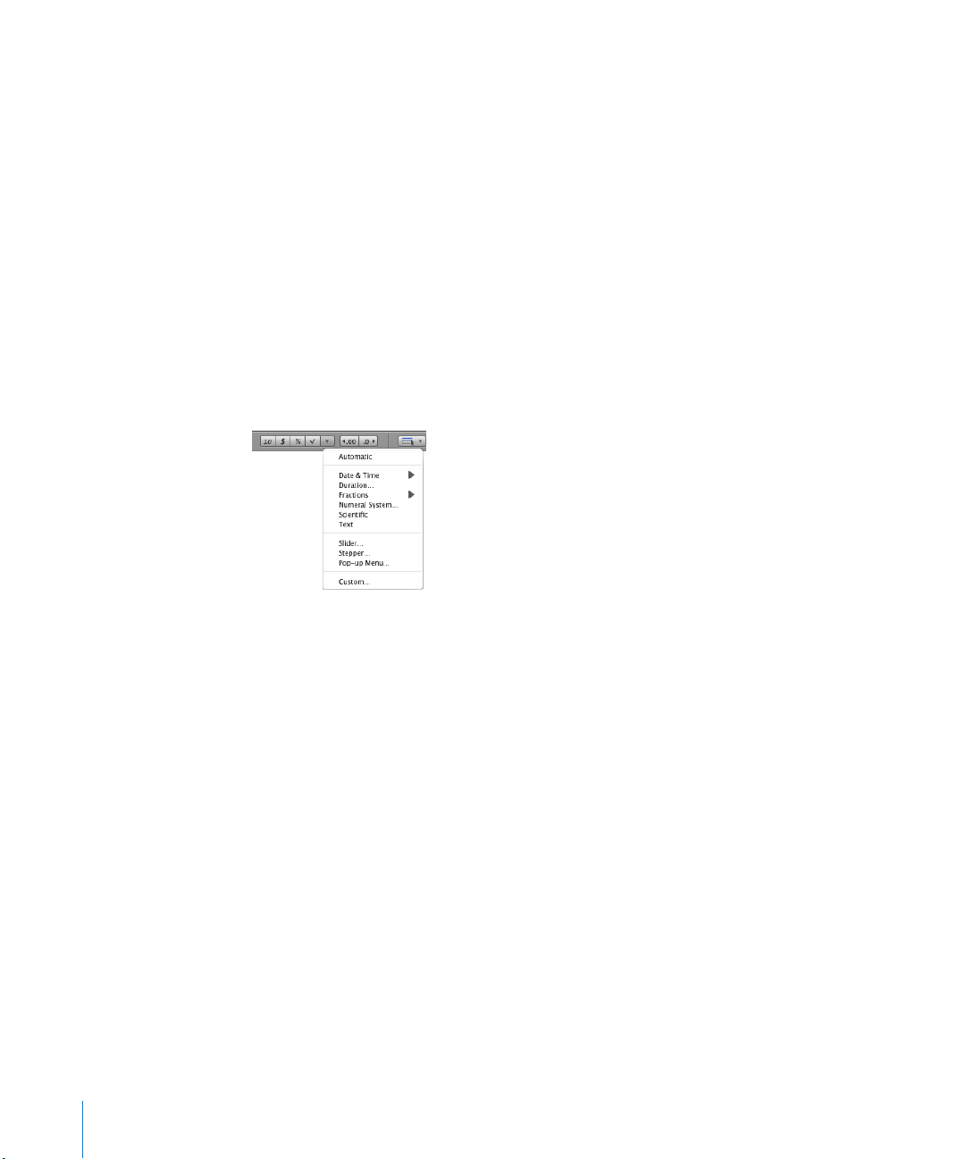
For more control over the number of decimal places, use the Cells inspector.

To dene a scientic format for one or more cells using the Cells inspector:

1 Select the cell or cells.

2 Click Inspector in the toolbar, and then click the Cells inspector button.

3 Choose Scientic from the Cell Format pop-up menu.

4 Use the Decimals eld to specify the number of decimal places to display.

Using the Text Format in Table Cells

Use the text format when you want all of a cell’s content to be treated as text, even when it’s a number. When a text format is applied to a cell, its value is displayed exactly as you type it.

Here are ways to dene a text format for one or more selected cells:

Click the Cell Formats button in the format bar and then choose Text. m

Click Inspector in the toolbar, click the Cells inspector button, and then choose Text m from the Cell Format pop-up menu.

Using a Checkbox, Slider, Stepper, or Pop-Up Menu in Table Cells

You can add a checkbox, slider, stepper, or pop-up menu to a cell:

Checkbox: Useful for cells whose value indicates one of two states, such as on or o, or yes or no.

Slider: Useful for quickly making large changes to numbers so you can see the eects

of the changes on other cells in the table or on a chart.

Stepper: Use to increase or decrease numbers in specic increments.

Pop-up menu: Use to predene the values a cell can contain.

When a cell is formatted to use a checkbox or pop-up menu, you can add or change a cell’s content only by using the control. Cells that use a slider or stepper let you type a value into the cell or use the control.

Here are ways to add controls to cells:

To add a checkbox, select the cell or cells. m

96 Chapter 4 Working with Table Cells

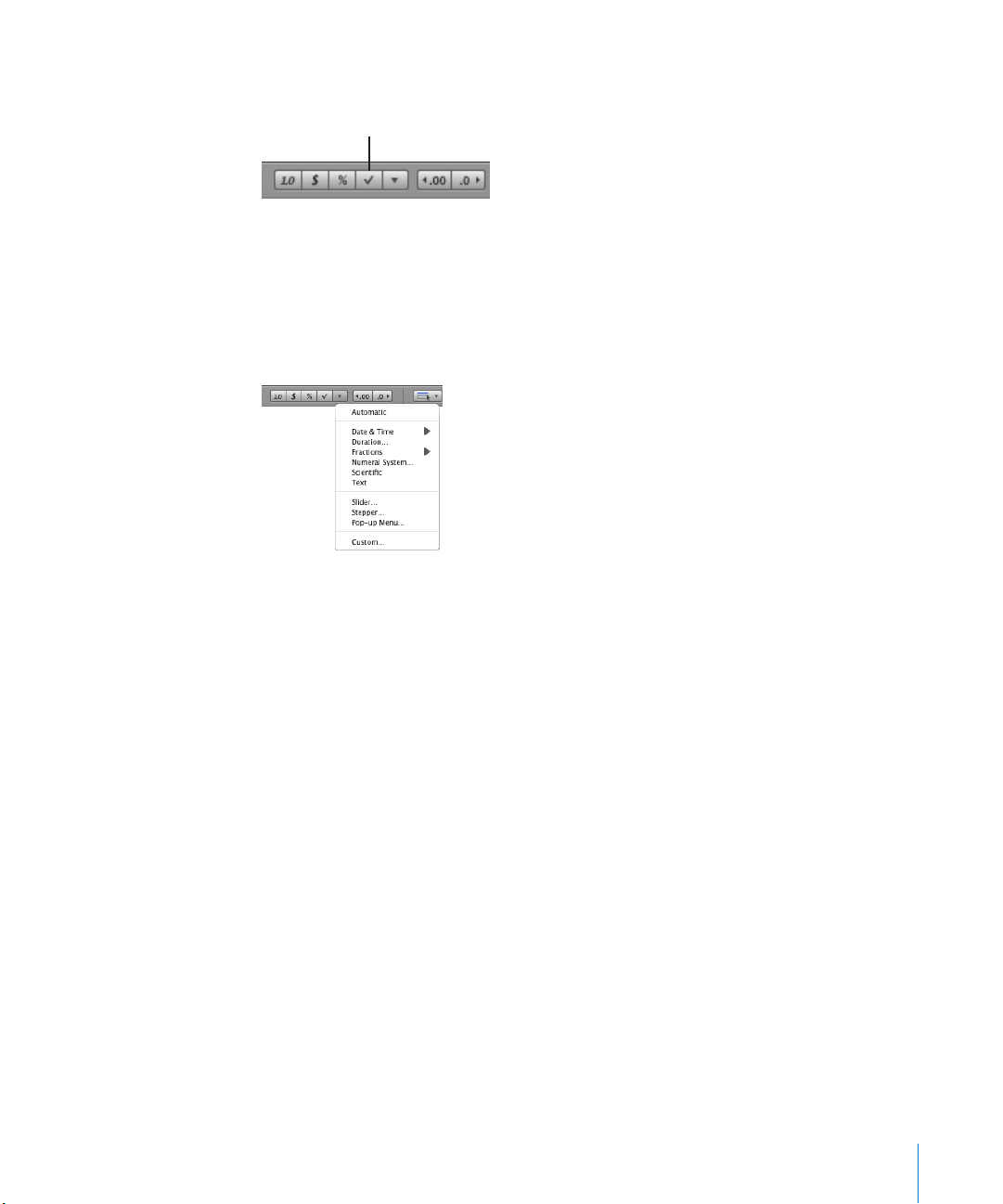
Click the Checkbox button in the format bar. Unchecked checkboxes are added to

Checkbox button

selected cells.

You can also click Inspector in the toolbar, and then click the Cells inspector button. Choose Checkbox from the Cell Format pop-up menu, and then select the initial state (Checked or Unchecked).

To add a slider, click the Cell Formats button in the format bar and then choose Slider m from the pop-up menu. A slider with default settings, visible in the Cells inspector, is created.

You can also open the Cells inspector and choose Slider from the Cell Format pop-up menu.

In the Cells inspector, change default settings if desired:

Minimum and Maximum: Indicates the lowest and highest cell values.

Increment: Indicates the amount by which the cell value increases or decreases when

you move the slider (or arrow keys) one increment.

Position: Lets you locate the slider to the right of the cell or at the bottom of the cell.

Display as: Applies a number, currency, percentage, fraction, scientic, or numeral

system format to the cell values.

Decimals: Indicates how many decimal places to display.

To add a pop-up menu, click the Cell Formats button in the format bar and then m choose Pop-up Menu to create a pop-up menu with default settings.

You can also open the Cells inspector and choose Pop-up Menu from the Cell Format pop-up menu.

In the Cells inspector, edit the placeholder entries in the list by selecting them and typing values of your choice.

To add an item to the list, click the Add button (+) and type the item. If you specify a number, it’s treated as a number, not as text.

Chapter 4 Working with Table Cells 97

To remove an item, select it and click the Delete button (–).

To add a stepper, click the Cell Formats button in the format bar and then choose m Stepper in the pop-up menu to create a stepper with default settings.

You can also open the Cells inspector and choose Stepper from the Cell Format popup menu.

In the Cells inspector, change the default settings if desired:

Minimum and Maximum: Indicates the lowest and highest cell values.

Increment: Indicates the amount by which the cell value increases or decreases when

you click the stepper control (or an arrow key) once.

Display as: Applies a number, currency, percentage, fraction, scientic, or numeral

system format to the cell values.

Decimals: Indicates how many decimal places to display.

Using Your Own Formats for Displaying Values in Table Cells

You can create your own cell formats for displaying numbers, text, and date and time values. Cell formats you create, called custom formats, are listed in the Cell Formats pop-up menu in the format bar.

Custom formats are also listed in the Cell Format pop-up menu in the Cells inspector.

To learn how to Go to

Dene a custom number format that applies

currency, decimal digit, and other display formatting to a number in a table cell

Dene custom number formatting that varies

with the value of a number in a table cell

Dene a custom date/time format, which species day, month, year, hour, minute, and other

aspects of a date/time value in a table cell

Dene text you want to appear next to a value

entered into a table cell

Manage the custom formats you create “Changing a Custom Cell Format” on page 109

“Creating a Custom Number Format” on page 99

“Dening the Integers Element of a Custom Number Format” on page 101

“Dening the Decimals Element of a Custom Number Format” on page 102

“Dening the Scale of a Custom Number Format” on page 103

“Associating Conditions with a Custom Number Format” on page 105

“Creating a Custom Date/Time Format” on page 107

“Creating a Custom Text Format” on page 108

“Reordering, Renaming, and Deleting Custom Cell Formats” on page 11 0

98 Chapter 4 Working with Table Cells

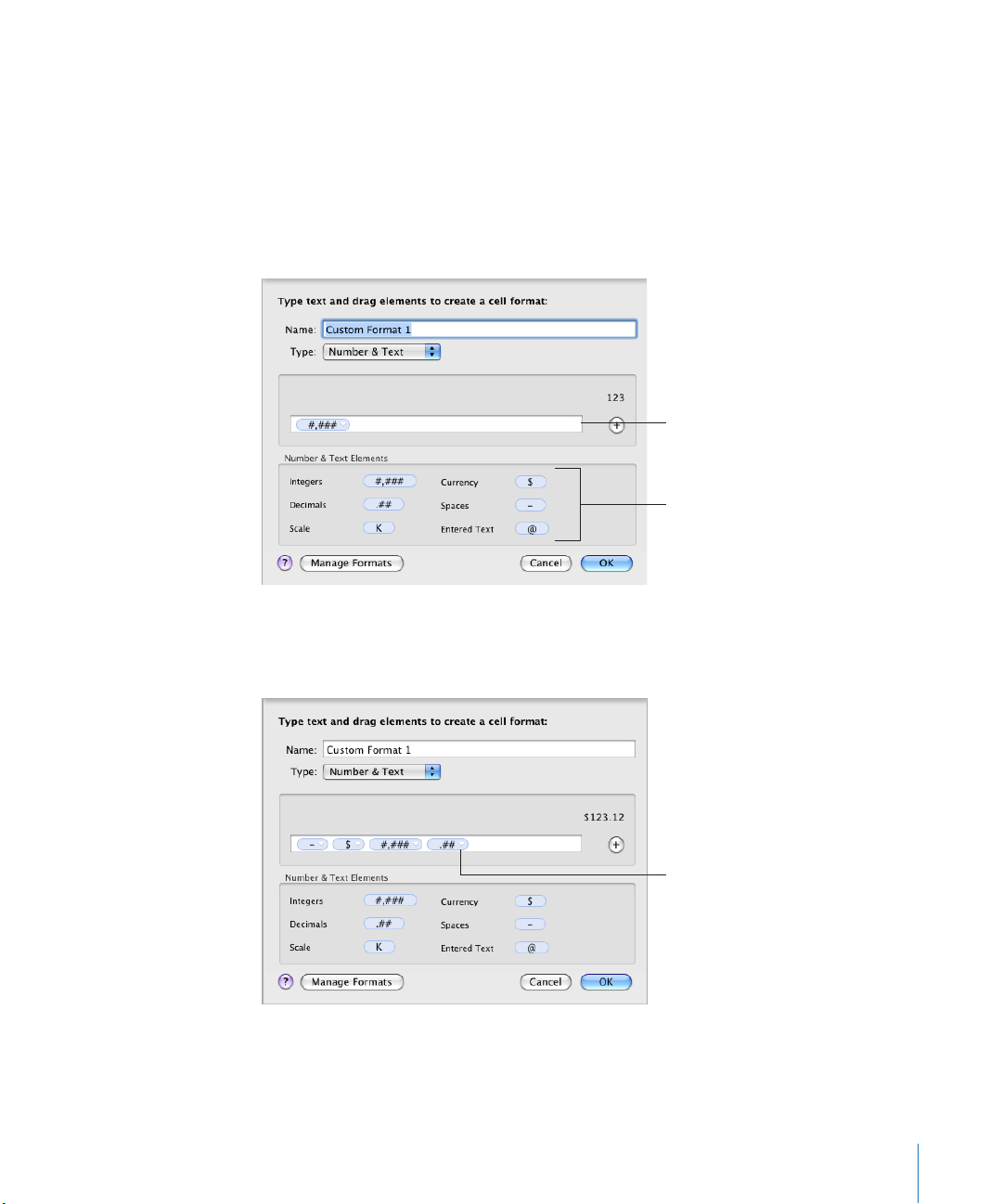
Creating a Custom Number Format

Format field

Drag the elements to the format field.

Click a disclosure triangle to choose a formatting option.

To dene your own display format for numbers in table cells:

1 Select one or more cells.

2 Do one of the following:

Choose Custom from the Cell Formats pop-up menu in the format bar. Â

Choose Custom from the Cell Format pop-up menu in the Cells inspector. Â

Choose Format > Create Custom Cell Format. Â

3 From the Type pop-up menu, choose Number & Text.

4 Dene your number format by dragging the (blue) elements from the Number & Text

Elements box into the format eld above the box.

Integers: Add this element when you want to format digits to the left of a decimal point. See “Dening the Integers Element of a Custom Number Format” on page 101 for more information.

Chapter 4 Working with Table Cells 99

Currency: Add this element to display a currency symbol. To identify the symbol you

want to use, click the disclosure triangle visible on the element when it’s in the format

eld and choose a symbol. You can maximize the choices in the pop-up menu by

selecting “Show complete list of currencies in Cells inspector” in Numbers preferences.

Decimals: Add this element to format how decimal digits are displayed. See “Dening the Decimals Element of a Custom Number Format” on page 102 for more information.

Spaces: Use this element to control the amount of space displayed between elements.

Click the disclosure triangle visible on the element when it’s in the format eld and

choose an option. Normal adds a standard space, Wide adds an em space, and Narrow adds a sixth of an em space. You can add more than one Spaces element to the format

eld with these options, but only one of the Spaces elements can be Flexible; this

option left-aligns the elements that precede it and right-aligns elements that follow it.

Scale: Use this element to size the display value of a number. For example, you can display values over 100 as number of hundreds (1000 displays as 10). See “Dening the Scale of a Custom Number Format” on page 103 for more information.

5 To display predened text before or after any element, place an insertion point in the

format eld and then type your text. You can click any element and use the Left Arrow

and Right Arrow keys to place the insertion point.

6 To delete an element in the eld, select it and then press Delete.

To move the element around in the eld, drag it.

7 In the Name eld, type a name for your number format.

Custom format names are listed in the Cell Formats pop-up menu in the format bar and in the Cell Format pop-up menu of the Cells inspector.

8 Click OK to save your number format and apply it to the selected cells.

Here’s an example of a number format:

Balance:-$ #,### .##

The hyphen is a Spaces element, set to display one Normal space between the Â currency symbol and the number.

The dollar sign is a Currency element. Â

#,### is an Integers element that displays numbers greater than 999 with a Â thousands separator.

.## is a Decimals element. Â

10 0 Chapter 4 Working with Table Cells

Apple NUMBERS User Manual 2009

Specifications and Main Features

Frequently Asked Questions

User Manual

Contents

Spreadsheet Templates

The Numbers Window

Zooming In or Out

The Sheets Pane

Print View

The Toolbar

The Format Bar

The Inspector Window

Formula Tools

The Styles Pane

The Media Browser

The Colors Window

The Fonts Window

The Warnings Window

Keyboard Shortcuts and Shortcut Menus

Creating a New Spreadsheet

Importing a Document from Another Application

Using CSV or OFX Files in a Spreadsheet

Opening an Existing Spreadsheet

Password-Protecting a Spreadsheet

Saving Spreadsheets

Undoing Changes

Automatically Saving a Backup Version

Saving a Spreadsheet as a Template

Saving Spotlight Search Terms for a Spreadsheet

Saving a Copy of a Spreadsheet

Closing a Spreadsheet Without Quitting Numbers

Using Sheets to Organize a Spreadsheet

Adding and Deleting Sheets

Reorganizing Sheets and Their Contents

Changing Sheet Names

Dividing a Sheet into Pages

Setting a Spreadsheet’s Page Size

Adding Headers and Footers to a Sheet

Arranging Objects on a Page in Print View

Setting Page Orientation

Setting Pagination Order

Numbering Pages

Setting Page Margins

Working with Tables

Adding a Table

Using Table Tools

Resizing a Table

Moving Tables

Naming Tables

Enhancing the Appearance of Tables

Copying Tables Among iWork Applications

Selecting Tables and Their Components

Selecting a Table

Selecting a Table Cell

Selecting a Group of Table Cells

Selecting a Row or Column in a Table

Selecting Table Cell Borders

Working with Rows and Columns in Tables

Adding Rows to a Table

Adding Columns to a Table

Rearranging Rows and Columns

Deleting Table Rows and Columns

Adding Table Header Rows or Header Columns

Freezing Table Header Rows and Header Columns

Adding Table Footer Rows

Resizing Table Rows and Columns

Alternating Table Row Colors

Hiding Table Rows and Columns

Sorting Rows in a Table

Filtering Rows in a Table

Creating Table Categories

Removing Table Categories and Subcategories

Managing Table Categories and Subcategories

Putting Content into Table Cells

Adding and Editing Table Cell Values

Working with Text in Table Cells

Working with Numbers in Table Cells

Displaying Content Too Large for Its Table Cell

Using Conditional Formatting to Monitor Table Cell Values