Texas instruments TI-86 Inferential Statistics and Distribution Functions

TI-86 Inferential Statistics and

Distribution Functions

Loading and Installing Inferential Statistics and

Distribution Features on Your TI-86...............................................................2

Loading the Inferential Statistics and Distribution Features into TI-86 Memory................................. 2

Installing the Inferential Statistics and Distribution Features for Use.................................................2

Displaying the STAT (Inferential Statistics and Distribution) Menu..................................................... 3

The STAT Menu................................................................................................................................... 3

Uninstalling the Inferential Statistics and Distribution Features.........................................................3

Deleting the Inferential Statistics and Distribution Program from TI-86 Memory...............................4

Example: Mean Height of a Population ......................................................... 4

Interpreting the Results......................................................................................................................5

Inferential Statistics Editors ........................................................................... 7

Displaying the Inferential Statistics Editors.........................................................................................7

Using an Inferential Statistics Editor...................................................................................................7

Bypassing the Inferential Statistics Editors.........................................................................................8

Inferential Statistics Editors for the STAT TESTS Instructions ....................9

STAT TESTS (Inferential Statistics Tests) Menu...................................................................................9

Inferential Statistics and Distribution Input Descriptions.........................24

Test and Interval Output Variables.............................................................. 26

Distribution (DISTR) Functions......................................................................28

STAT DISTR (Inferential Statistics Distribution) Menu.......................................................................28

DRAW (Distribution Shading) Functions ...................................................... 33

STAT DRAW (Inferential Statistics Draw) Menu................................................................................33

FUNC (Function) Parameters ......................................................................... 35

STAT FUNC (Inferential Statistics Functions) Menu.......................................................................... 35

Menu Map for Inferential Statistics and Distribution Functions .............. 39

MATH menu (where STAT is automatically placed)..........................................................................39

(MATH) STAT (Inferential Statistics and Distribution) Menu.............................................................39

STAT TESTS (Inferential Statistics Tests) Menu.................................................................................39

STAT DISTR (Inferential Statistics Distribution) Menu.......................................................................39

STAT DRAW (Inferential Statistics Draw) Menu................................................................................39

STAT FUNC (Inferential Statistics Functions) Menu.......................................................................... 39

Assembly Language Programming: Inferential Statistics and Distribution Functions

Loading and Installing Inferential Statistics and Distribution Features on Your TI-86

To load the inferential statistics and distribution features onto your TI-86, you need a computer and the TI-86 Graph Link software and cable. You also need to download the statistics program file from the Internet and save it on your computer.

Loading the Inferential Statistics and Distribution Features into TI-86 Memory

When sending a program from your computer to the TI-86, the calculator must no be in Receive mode. The Receive mode is used when sending programs or data from one calculator to another.

Start the TI-86 Graph Link on your computer.

Turn on your TI-86 and display the home screen.

Click on the Send button on the TI-86 Graph Link toolbar to display the Send dialog box.

WLink86.exe

- l

Other files associated with the assembly language program (

statedit

PRGM NAMES

need not do anything with them.

For assembly language programs that must be installed, up to three can be installed at a time (although the TI-86 can store as many as permitted by memory). To install a fourth, you must first uninstall (page 3) one of the others.

exstats, exstats2

) appear on the

menu, but you

Specify the statistics program file as the file you want to send.

Send the program to the TI-86. The program and its associated executable file become items on

PRGM NAMES

the

Exit Graph Link.

menu.

infstat1.86g

Installing the Inferential Statistics and Distribution Features for Use

Use the assembly language program

Infstats

to install the inferential statistics and distribution features directly into the TI-86’s built-in functions and menus. After installation, the inferential statistics and distribution features are available each time you turn on the calculator. You do not need to reinstall them each time. When you run assembly language programs that do not install themselves into the

- Œ / menu, their features are lost when you turn off the calculator.

All examples assume that on your TI-86. The position of

Infstats

STAT

is the only assembly language program installed

on the

MATH

menu may vary, depending on

how many other assembly language programs are installed.

Asm(

Select to paste it to a blank line on the home screen.

Select

NAMES

to the home screen as an argument.

from the

Infstat

from the

menu to paste

CATALOG

PRGM

Infstats

- w & #

(move 4 to

Asm(

)

8 &

Infstat

(select

Assembly Language Programming: Inferential Statistics and Distribution Functions

The variables that will be overwritten are listed on page 26.

If other assembly language programs are installed, may be in a menu cell other

- Œ / '

than

STAT

Run the installation program.

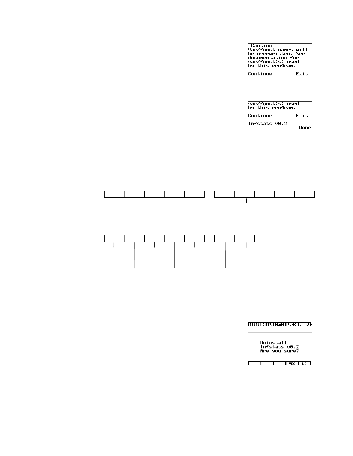
Caution:

If you have values

stored to variables used by the statistical features, they will be overwritten. To save your values, press * to exit, store them to different variables, and then repeat this installation.

Continue the installation. Your

version number may differ from the one shown in the example.

Display the home screen.

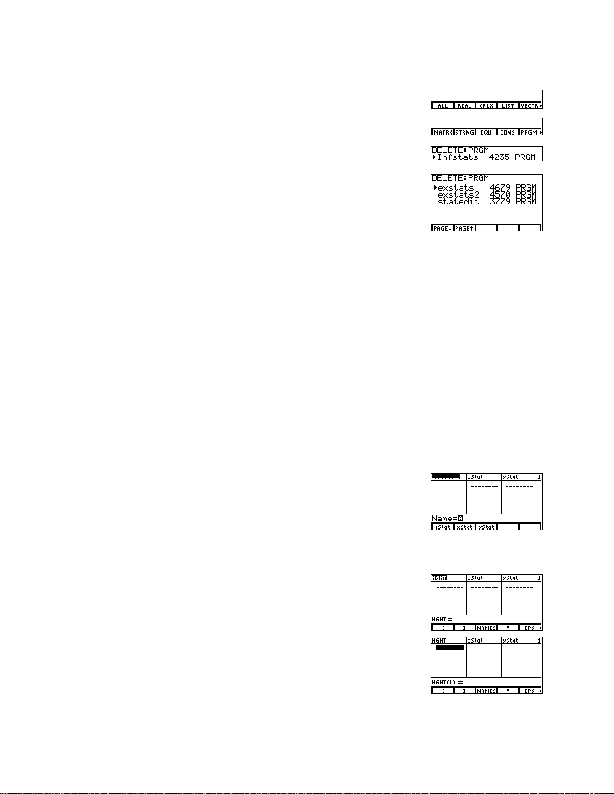
Displaying the STAT (Inferential Statistics and Distribution) Menu - Œ /

When you install the inferential statistics and distribution program on your TI-86 and activate it,

NUM PROB ANGLE HYP MISC 4 INTER STAT

STAT

becomes the last item on the

Inferential Statistics and Distribution Menu

MATH

menu.

When you uninstall the inferential statistics and distribution features, the statistics assembly language programs (

exstats2,

remain in memory, but the

STAT

the

Infstats, exstats,

statedit

and

option is removed from

MATH

menu.

)

The STAT Menu - Œ / '

TESTS DISTR DRAW FUNC Uninst 4 RsltOn RsltOf

Inferential Distribution Uninstall Results Off Statistics Shading Instruction (Default) Test Editors

Functions Statistics (Intermediate calculation

Distribution Inferential Results On

Test Functions results display)

Uninstalling the Inferential Statistics and Distribution Features

Display the then select

If you are sure you want to uninstall, select confirmation menu. The menu is removed and the home screen is displayed. Your version number may differ from the one shown in the example.

STAT

Uninst

menu, and

Yes

from the

- Œ / ' *

)

STAT

Assembly Language Programming: Inferential Statistics and Distribution Functions

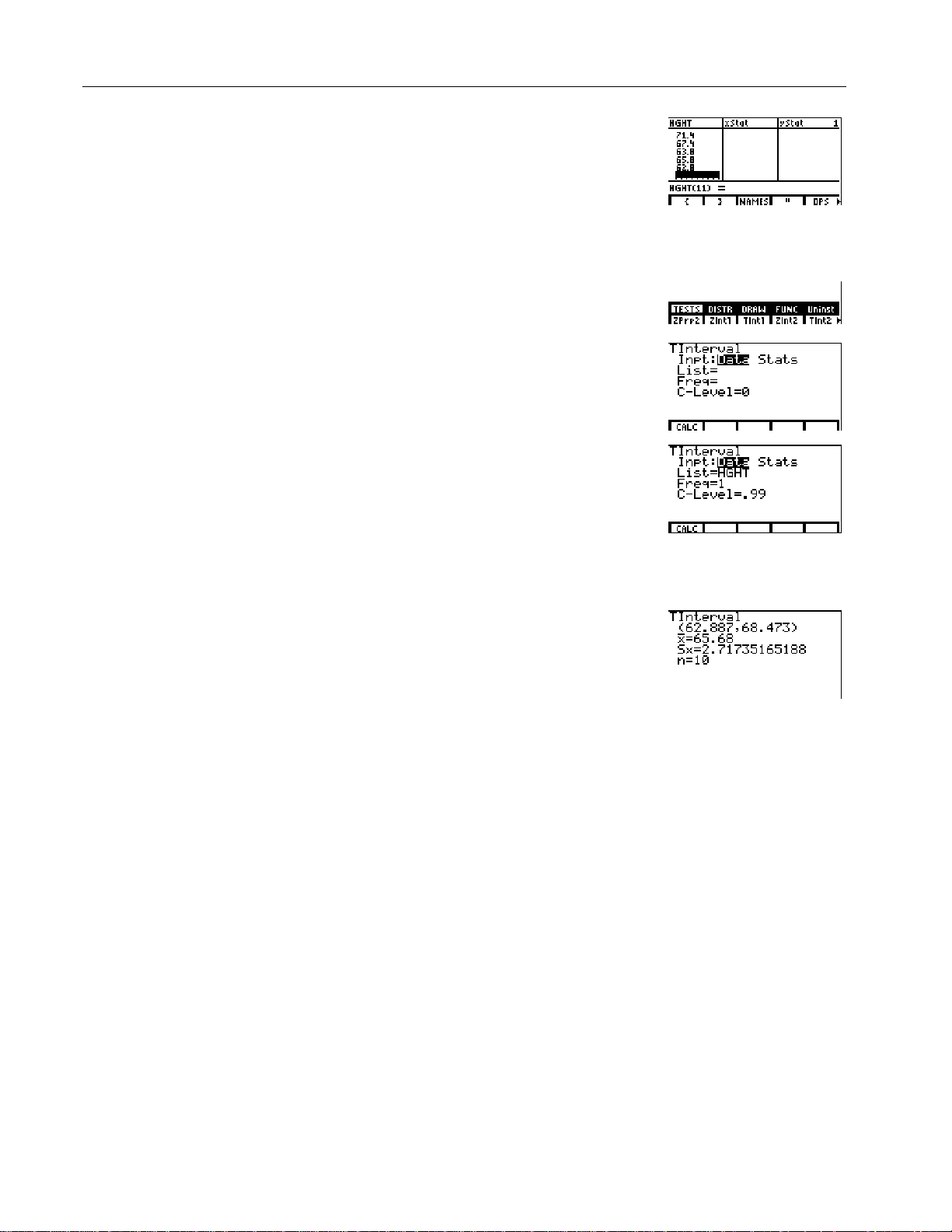
Deleting the Inferential Statistics and Distribution Program from TI-86 Memory

Deleting the program does not delete the variables associated with the program.

Select menu.

Select

DELET

PRGM

menu.

from the

MEM

- ™ '

/ *

Move the selection cursor to

Infstats

Move the selection cursor to

exstats

down and delete

statedit

Display the home screen.

, and then delete it.

and then delete it. Scroll

exstats2

and

(as needed)

Example: Mean Height of a Population

Estimate the mean height of a population of women, given the random sample below. Because heights among a biological population tend to be normally distributed, a t distribution confidence interval can be used when estimating the mean. The 10 height values below are the first 10 of 90 values, randomly generated from a normally distributed population with an assumed mean of 65 inches and a standard deviation of 2.5 inches.

This example uses an inferential statistics editor. An editor prompts you for test information. See page 7 for another example of using an inferential statistics editor. You can also enter test parameters without using an editor. See page 8 for an example of bypassing the inferential statistics editors.

Height (in Inches) of Each of 10 Women

66.7 66.3 62.8 66.9 62.9 71.4 67.4 63.8 65.8 62.8

Create a new list column. The cursor indicates that alpha-lock is on. The existing list name columns shift to the right.

Note:

Your statistics editor may not look like the one pictured here, depending on the lists you have already stored.

Enter the list name at the prompt. The list to which you will store the women’s height data is created.

Move the cursor onto the first row of the list. displayed on the bottom line.

HGHT(1)=

Name=

- š ' }

y p

[H] [G] [H] [T]

†

Assembly Language Programming: Inferential Statistics and Distribution Functions

Enter the first height value. As you enter it, it is displayed on the bottom line.

The value is displayed in the first row, and the rectangular cursor moves to the next row. Enter the other nine height values the same way.

Display the inferential statistics

TInterval

editor for the

Select

Enter the test requirements:

Calculate are displayed on the home screen.

Note:

the screen.

TIntl

(

STAT TESTS

Data

Set alpha-lock and enter the

List

name.

Enter 1 at the

Enter a 99 percent confidence level at the

C-Level=

Press .,

to clear the results from

menu.

Inpt

in the

Freq=

prompt.

the test. The results

. - Œ

) from

field. If

prompt.

, or

/ ' & / (

press |

† 1 1

[H] [G] [H] [T]

†

† Ë

Stats

is selected,

Interpreting the Results

The first line

(62.887,68.473)

shows that the 99 percent confidence interval for the population mean is between about 62.9 inches (5 feet 2.9 inches) and 68.5 inches (5 feet 8.5 inches). This is about a 5.6-inch spread.

The .99 confidence level indicates that in a very large number of samples, we expect 99 percent of the intervals calculated to contain the population mean. The actual mean of the population sampled is 65 inches, which is in the calculated interval.

The second line gives the mean height of the sample þ used to compute this interval. The third line gives the sample standard deviation gives the sample size

. The bottom line

To obtain a more precise bound on the population mean m of women’s heights, increase the sample size to 90. Use a sample mean þ of 64.5 and sample standard deviation

Stats

(summary statistics) input option.

of 2.8 calculated from the larger random sample. This time, use the

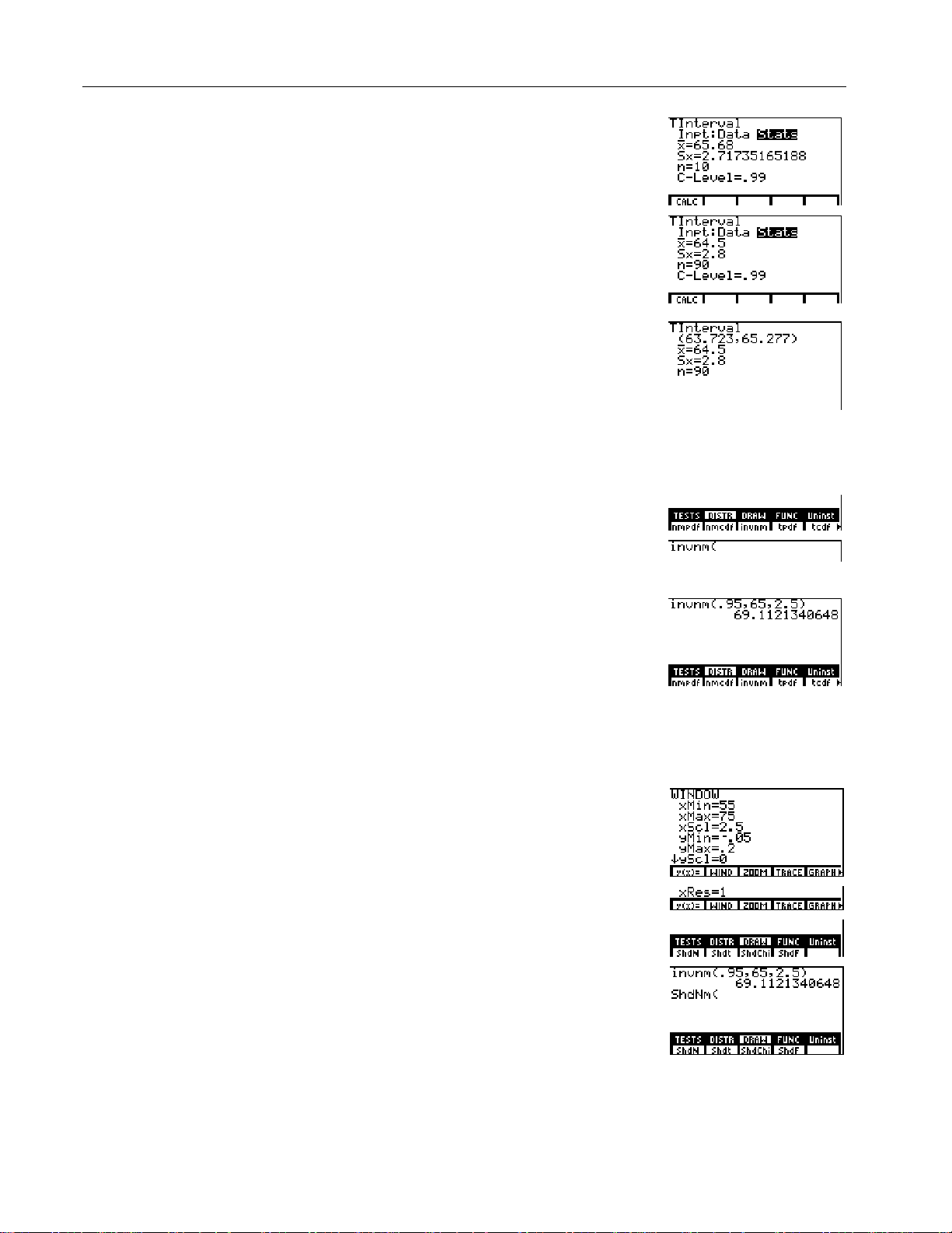
Assembly Language Programming: Inferential Statistics and Distribution Functions

The parameters are

invnm(

area[, m, s

]).

Display the inferential statistics and distribution editor for and select

Enter the test requirements:

Store 64.5 to

Store 2.8 to

Store 90 to

Calculate the test. The

Stats

in the

Inpt

results

TIntl

field.

: - Œ / ' & / ( ~ Í

Ë 5

†

Ë 8

are displayed on the home screen.

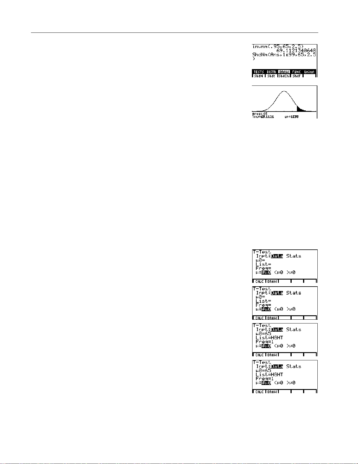
If the height distribution among a population of women is normally distributed with a mean

of 65 inches and a standard deviation σ of 2.5 inches, what height is

exceeded by only 5 percent of the women (the 95th percentile)?

invnm(

invnm

STAT DISTR

to the home

stands for

‘ y Œ

/ ' '

(

Display the (Distributions) menu.

Paste screen. ( Inverse Normal.)

Enter .95 as the area, 65 as µ, and 2.5 as σ.

The result is displayed on the home screen; it shows that five percent of the women are taller than 69.1 inches (5 feet 9.1 inches).

Now graph and shade the top five percent of the population.

Set the window variables to these values:

xMin=55 yMin=L.05 xRes=1 xMax=75 yMax=.2 xScl=2.5 yScl=0

Display the

Paste screen. (

STAT DRAW

ShdNm(

ShdNm

to the home

stands for Shade

Normal.)

menu.

6 '

. y Œ / ' (

Assembly Language Programming: Inferential Statistics and Distribution Functions

The parameters are

ShdNm(

upperbound

lowerbound,

, m, s

[

The answer (

)

]

from step 14 is the lower bound. 1å99 is the upper bound. The

Ans

69.1121340648)

y ¡ ¢

¢ 65 ¢ 2 Ë

normal curve is defined by a mean µ of 65 and a standard deviation σ of 2.5.

Plot and shade the normal curve.

Area=

is the area above the 95th percentile. bound.

low=

is the lower

up=

is the upper bound.

You can remove the menu from the bottom of the screen.

Inferential Statistics Editors

Displaying the Inferential Statistics Editors

When you select a hypothesis test or confidence interval instruction from the home screen, the appropriate inferential statistics editor is displayed. The editors vary according to each test or interval’s input requirements.

When you select the

ANOVA(

instruction, it is pasted to the home screen.

does not have an editor screen.

ANOVA(

Data

Select lists as input. Select enter summary statistics, such as v, Sx, and n as inputs.

Most of the inferential statistics editors for the hypothesis tests prompt you to select one of three alternative hypotheses.

to enter the data

Stats

Using an Inferential Statistics Editor

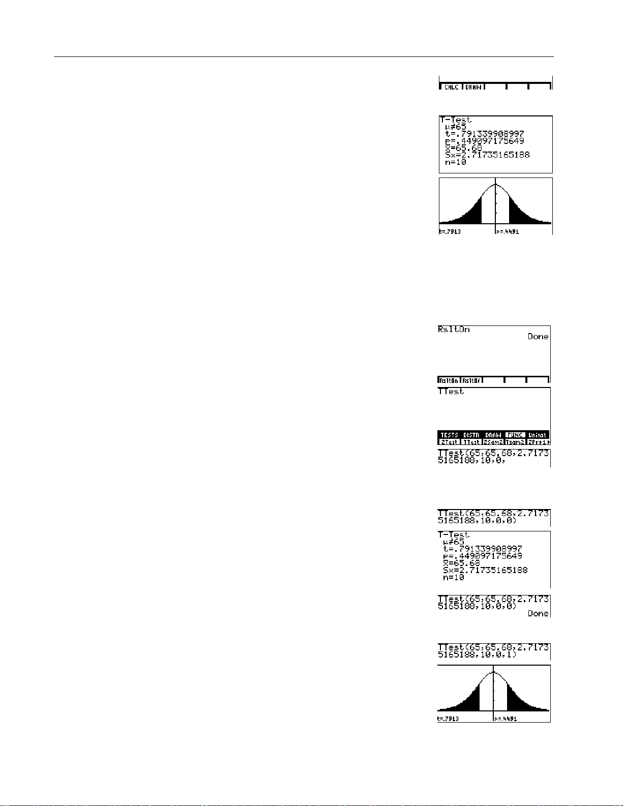
This example uses the inferential statistics editor for

Select a hypothesis test or confidence interval from the

STAT TESTS

menu. The

appropriate editor displays.

Select

Data

Stats

input, if the

selection is available.

Enter real numbers, list names, or expressions for each argument in the editor. See the input descriptions table on page 24.

Select the alternative hypothesis against which to test, if the selection is available.

- Œ / ' & '

(displays

TTest

the

[H] [G] [H] [T]

or !

editor)

TTest

Assembly Language Programming: Inferential Statistics and Distribution Functions

Select No or Pooled option, if the selection is available. The Pooled option is available for

TInt2

and

! b

¦ Select

want the variances pooled. Population variances can be unequal.

¦ Select

variances pooled. Population variances are assumed to be equal.

Yes

for the

only. Press " or

to select an option.

if you do not

Yes

if you want the

Tsam2

Select

Calc

Draw

(when Draw

is available) to execute the instruction.

When you select results are displayed on the

Calc

, the

home screen.

When you select

Draw

, the

results are displayed in a graph (not available for a confidence interval).

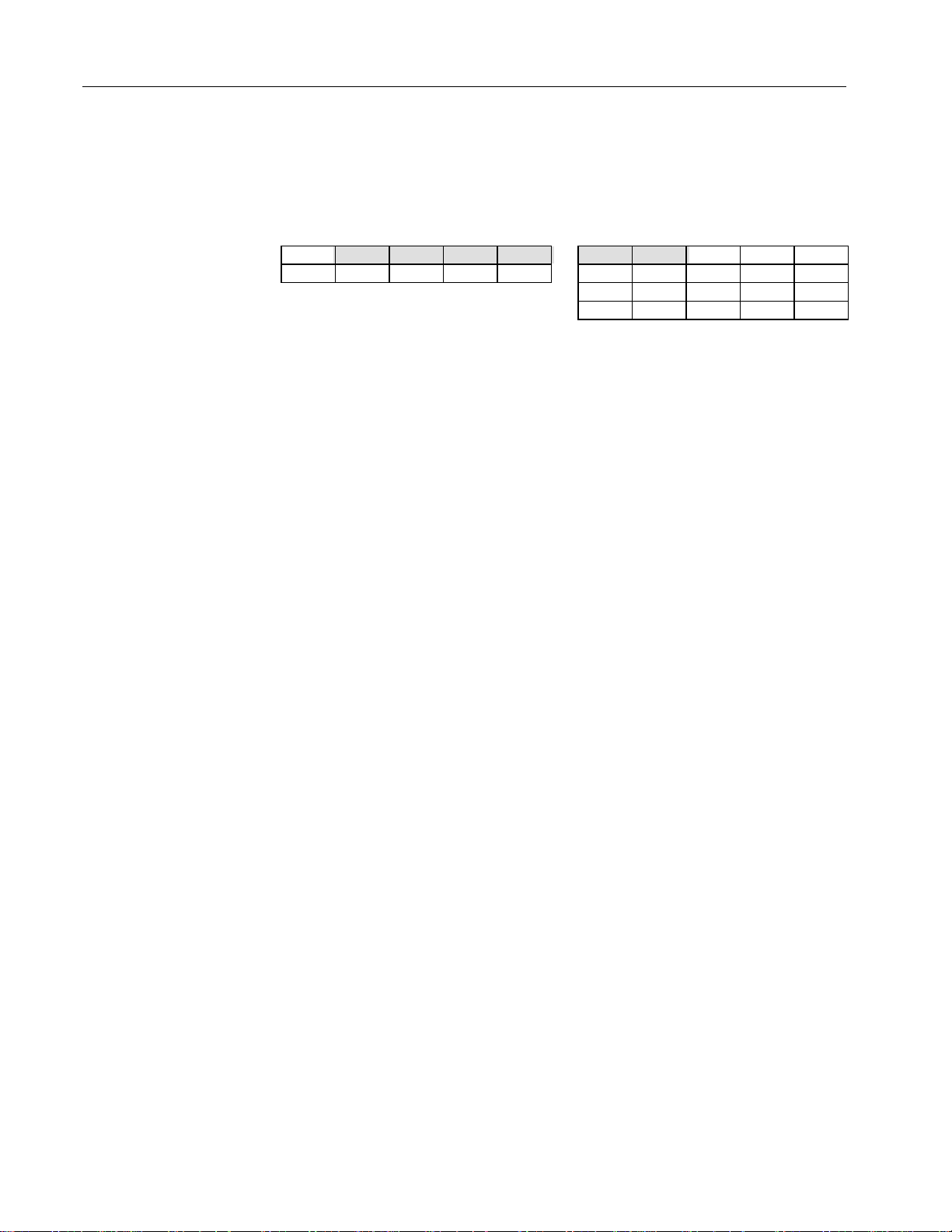
Bypassing the Inferential Statistics Editors

You can paste a hypothesis test or confidence interval instruction to the home screen without displaying the corresponding inferential statistics editor. You can also paste a hypothesis test or confidence interval instruction to a command line in a program.

RsltOn

Turn

Note:

The default is

(Results Off).

(Results On).

RsltOf

- Œ / ' / & b

This example uses summary statistics. See pages 35-38 for a list of menu parameters.

FUNC

(Function)

Select the instruction from the

STAT FUNC

Input the syntax for each

menu.

hypothesis test and confidence interval instruction. Complete the syntax by using one of the options below:

Enter 0 (zero) as the last parameter to display the results on the home screen.

Note:

The home screen does

not display the results if you

RsltOf

use

– or –

Enter 1 as the last parameter to display the results in a graph. The graph is drawn whether you use

RsltOf

RsltOn

: / ) '

(for the

TTest

instruction)

65 P 65.68

2.71735165188 0

E b

You can remove the menu from the bottom of the screen.

Assembly Language Programming: Inferential Statistics and Distribution Functions

Inferential Statistics Editors for the STAT TESTS Instructions

STAT TESTS (Inferential Statistics Tests) Menu - Œ / ' &

TESTS DISTR DRAW FUNC Uninst

ZTest TTest Zsam2 Tsam2 ZPrp1

RsltOn RsltOf

ZPrp2 ZIntl TIntl ZInt2 TInt2

ZPin1 ZPin2 Chitst FSam2 TLinR

ANOVA

Test Name Description Function

ZTest TTest Zsam2 Tsam2 ZPrp1 ZPrp2 ZIntl

TIntl

ZInt2

TInt2

ZPin1

ZPin2

Chitst FSam2 TLinR ANOVA

One-sample Z-test Test for one m , known

One-sample t-test Test for one m, unknown

Two-sample Z-test Test comparing two m’s, known s’s

Two-sample t-test Test comparing two m’s, unknown s’s

One-proportion Z-test Test for one proportion

Two- proportion Z-test Test comparing two proportions

One-sample Z confidence interval Confidence interval for one m,

known

One-sample t confidence interval Confidence interval for one m,

unknown

Two-sample Z confidence interval

Two-sample t confidence interval Confidence interval for difference of

One-proportion Z confidence interval

Two-proportion Z confidence interval

Chi-square test Chi-square test for two-way tables

Two-sample Û-test Test comparing two s’s

Linear regression t-test t-test for regression slope and

One-way analysis of variance One-way analysis of variance

Confidence interval for difference of two m’s, known s’s

two m’s, unknown s’s

Confidence interval for one proportion

Confidence interval for difference of two proportions

This section provides a description of each

STAT TESTS

instruction and shows the

unique inferential statistics editor for that instruction with example arguments.

Descriptions of instructions that offer the

Data/Stats

input choice show both

types of input screens. Descriptions of instructions that do not offer the

Data/Stats

input choice show

only one input screen.

The description then shows the unique output screen for that instruction with the example results.

Descriptions of instructions that offer the

Calculate/Draw

output choice show

both types of screens: calculated and drawn results. Descriptions of instructions that offer only the

Calculate

output choice show the

calculated results on the home screen.

Assembly Language Programming: Inferential Statistics and Distribution Functions

All examples on pages 10 through 23 assume a fixed-decimal mode setting of four. If you set the decimal mode to

Float

or a different fixed-decimal setting, your

output may differ from the output in the examples.

Be sure to turn off the y= functions before drawing results.

To remove the menu from a drawing, press :.

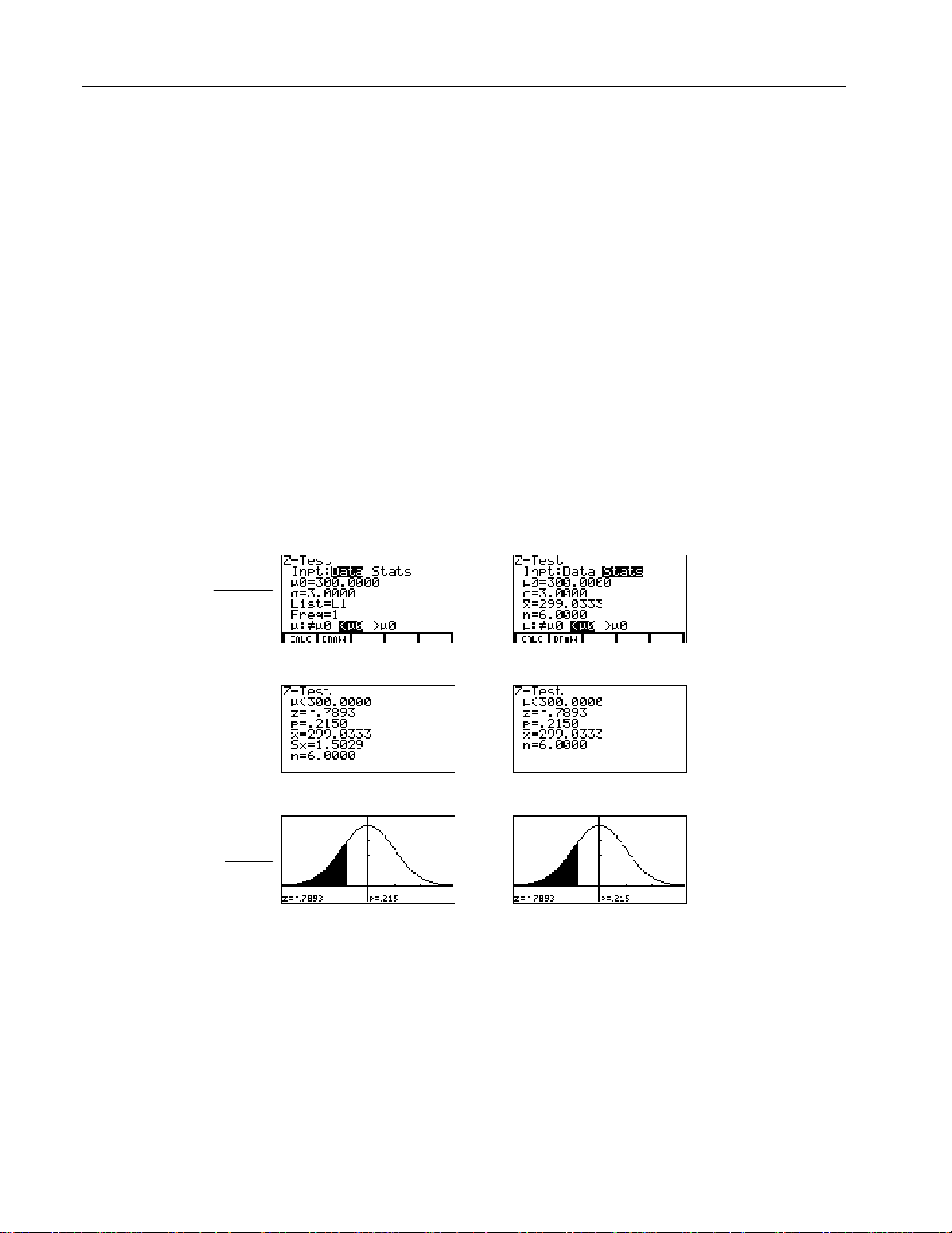
Ztest

Z-Test

This one-sample Z-test, shown as

in the editor, performs a hypothesis test for a single unknown population mean m when the population standard deviation

is known. It tests the null hypothesis H0: m=

alternatives below.

against one of the

Input

Calculate Results

mƒm

: m<

: m>

ƒm

(m:

)

(m:<

(m:>

)

In the example:

L1=

{299.4 297.7 301 298.9 300.2 297}

Data Stats

Drawn Results

Assembly Language Programming: Inferential Statistics and Distribution Functions

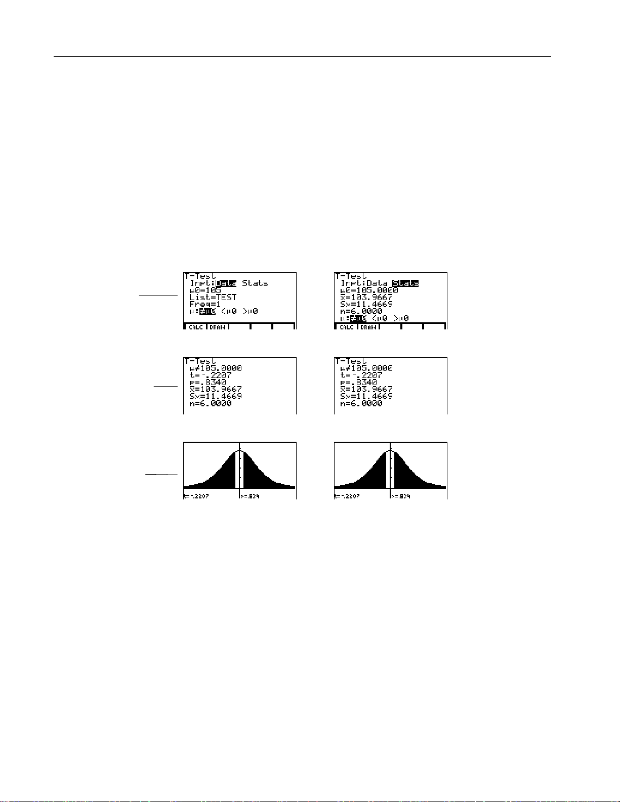
TTest

T-Test

This one-sample t-test, shown as

in the editor, performs a hypothesis test

for a single unknown population mean m when the population standard deviation

is unknown. It tests the null hypothesis H

below.

: m=

against one of the alternatives

Input

Calculate Results

mƒm

: m<

: m>

ƒm

(m:

)

(m:<

(m:>

)

In the example:

TEST=

{91.9 97.8 111.4 122.3 105.4 95}

Data Stats

Drawn Results

Assembly Language Programming: Inferential Statistics and Distribution Functions

Zsam2

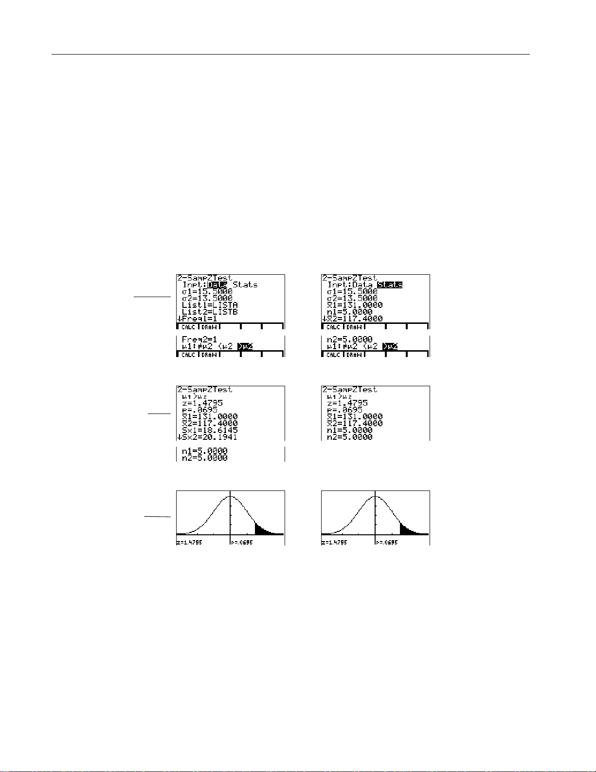
This two-sample Z-test, shown as the means of two populations ( both population standard deviations ( H

is tested against one of the alternatives below.

m m m

1ƒm2

(m1:ƒm2) (m1:<m2)

(m1:>m2)

2-SampZTest

and

) based on independent samples when

and

In the example:

in the editor, tests the equality of

) are known. The null hypothesis

Input

Calculate Results

LISTA= LISTB=

{154 109 137 115 140} {108 115 126 92 146}

Data Stats

Drawn Results

Assembly Language Programming: Inferential Statistics and Distribution Functions

Tsam2

and

2-SampTTest

) based on independent samples when

This two-sample t-test, shown as means of two populations ( neither population standard deviation ( H

is tested against one of the alternatives below.

m m m

1ƒm2

(m1:ƒm2) (m1:<m2)

(m1:>m2)

In the example:

in the editor, tests the equality of the

) is known. The null hypothesis

Input

Calculate Results

SAMP1= SAMP2=

{12.207 16.869 25.05 22.429 8.456 10.589} {11.074 9.686 12.064 9.351 8.182 6.642}

The pooled option is available for variances can be unequal.

Yes

means that population variances are assumed to be

equal.

Data Stats

Tsam2

and

TInt2

only. No means that population

Drawn Results

Assembly Language Programming: Inferential Statistics and Distribution Functions

ZPrp1

This one-proportion Z-test, shown as

1-PropZTest

an unknown proportion of successes (prop). It takes as input the count of successes in the sample x and the count of observations in the sample n. tests the null hypothesis H0: prop=p0 against one of the alternatives below.

: propƒp0

Input

: prop<p0

: prop>p0

(prop:ƒp0)

(prop:<p0)

(prop:>p0)

in the editor, computes a test for

ZPrp1

Calculate Results

Drawn Results

phat represents

Assembly Language Programming: Inferential Statistics and Distribution Functions

ZPrp2

This two-proportion Z-test, shown as

2-PropZTest

compare the proportion of successes (p1 and p2) from two populations. It takes as input the count of successes in each sample (x1 and x2) and the count of observations in each sample (n1 and n2).

ZPrp2

H0: p1=p2 (using the pooled sample proportion below.

in the editor, computes a test to

tests the null hypothesis

) against one of the alternatives

Input

Calculate Results

Drawn Results

Phat represents

: p

: p1<p2

: p1>p2

(p1:ƒp2)

(p1:<p2) (p1:>p2)

in the editor. Phat1 represents

phat1 represents phat2 represents phat represents

, and phat2 represents

Assembly Language Programming: Inferential Statistics and Distribution Functions

ZIntl

This one-sample Z confidence interval, shown as confidence interval for an unknown population mean m when the population standard deviation

is known. The computed confidence interval depends on the

user-specified confidence level.

In the example:

L1=

{299.4 297.7 301 298.9 300.2 297}

Data Stats

Input

Calculate Results

ZInterval

in the editor, computes a

Input

Calculate Results

TIntl

This one-sample t confidence interval, shown as

TInterval

in the editor, computes a confidence interval for an unknown population mean m when the population standard deviation s is unknown. The computed confidence interval depends on the user-specified confidence level.

In the example:

L6=

{1.6 1.7 1.8 1.9}

Data Stats

Assembly Language Programming: Inferential Statistics and Distribution Functions

ZInt2

This two-sample Z confidence interval, shown as computes a confidence interval for the difference between two population means (

) when both population standard deviations (

1Nm2

computed confidence interval depends on the user-specified confidence level.

In the example:

2-SampZInt

and

in the editor,

) are known. The

Input

Calculate Results

LISTC= LISTD=

{154 109 137 115 140} {108 115 126 92 146}

Data Stats

Assembly Language Programming: Inferential Statistics and Distribution Functions

TInt2

This two-sample t confidence interval, shown as computes a confidence interval for the difference between two population means (

) when both population standard deviations (

1Nm2

computed confidence interval depends on the user-specified confidence level.

In the example:

2-SampTInt

and

in the editor,

) are unknown. The

Input

Calculate Results

SAMP1= SAMP2=

{12.207 16.869 25.05 22.429 8.456 10.589} {11.074 9.686 12.064 9.351 8.182 6.642}

The pooled option is available for variances can be unequal.

means that population variances are assumed to be

Yes

equal.

Data Stats

TInt2

and

only. No means that population

Tsam2

Assembly Language Programming: Inferential Statistics and Distribution Functions

ZPin1

This one-proportion Z confidence interval, shown as computes a confidence interval for an unknown proportion of successes. It takes as input the count of successes in the sample x and the count of observations in the sample n. The computed confidence interval depends on the user-specified confidence level.

Input

Calculate Results

ZPin2

This two-proportion Z confidence interval, shown as computes a confidence interval for the difference between the proportion of successes in two populations (p each sample (x

and x2) and the count of observations in each sample (n1 and n2) .

The computed confidence interval depends on the user-specified confidence level.

). It takes as input the count of successes in

1-PropZInt

2-PropZInt

in the editor,

Input

Calculate Results

Assembly Language Programming: Inferential Statistics and Distribution Functions

Chitst

Chi

Test

This test, shown as

in the editor, computes a chi-square test for

association on the two-way table of counts in the matrix you specify at the

Observed

prompt. The null hypothesis H0 for a two-way table is: no association exists between row variables and column variables. The alternative hypothesis is: the variables are related.

Matrix Editor

Input

Calculate Results

Before computing a matrix variable name at the

Chitst

, enter the observed counts in a matrix. Enter that

Observed

prompt in the editor. At the

Expected

prompt, enter the matrix variable name to which you want the computed expected counts to be stored.

Note:

Press -

to select Matrix A from

the MATRX EDIT menu.

‰ '

[A]

Note:

Press -

to display Matrix B.

‰ '

[B]

Drawn Results

Assembly Language Programming: Inferential Statistics and Distribution Functions

ÜSam2 This two-sample Û-test, shown as

2-SampÜTest

compare two normal population standard deviations ( means and standard deviations are all unknown. sample variances Sx1

/Sx22, tests the null hypothesis H0:

alternatives below.

: : :

1ƒs2

(s1:ƒs2)

(s1:<s2)

(s1:>s2)

In the example:

in the editor, computes an Û-test to

and

Sam2

, which uses the ratio of

ÜÜ

). The population

against one of the

Input

Calculate Results

Drawn Results

SAMP4= SAMP5=

{7 L4 18 17 L3 L5 1 10 11 L2} {L1 12 L1 L3 3 L5 5 2 L11 L1 L3}

Data Stats

Assembly Language Programming: Inferential Statistics and Distribution Functions

TLinR

This linear regression t-test, shown as

LinRegTTest

regression on the given data and a t-test on the value of slope b and the correlation coefficient r for the equation y=a+bx. It tests the null hypothesis H

For the regression equation, you can use the fix-decimal mode setting to control the number of digits stored after the decimal point. However, limiting the number of digits to a small number could affect the accuracy of the fit.

(equivalently,

: bƒ0 and rƒ0

: b<0 and r<0

: b>0 and r>0

The regression equation is automatically stored to

/ '

). If you enter a y= variable name at the regression equation is automatically stored to the specified example below, the regression equation is stored to (turned on).

=0) against one of the alternatives below.

(b & r:ƒ0)

(

& r:<0)

(

& r:>0)

In the example:

L3=

{38 56 59 64 74}

L4=

{41 63 70 72 84}

Input

in the editor, computes a linear

: b=0

RegEQ

- š * /

(

prompt, the calculated

equation. In the

, which is then selected

Calculate Results

Assembly Language Programming: Inferential Statistics and Distribution Functions

ANOVA

This test computes a one-way analysis of variance for comparing the means of 2 to 20 populations. The ANOVA procedure for comparing these means involves analysis of the variation in the sample data. The null hypothesis H tested against the alternative H

ANOVA(

list1,list2

...,list20]

[

)

:. Not all

In the example:

L1=

7 4 6 6 5}

{

L2=

6 5 5 8 7}

{

L3=

{4 7 6 7 6}

Input

Intermediate calculation results display only when

Calculate Results

RsltOn is selected from the STAT menu.

...

are equal.

=...=

SS is sum of squares and MS is mean square.

Assembly Language Programming: Inferential Statistics and Distribution Functions

Inferential Statistics and Distribution Input Descriptions

This table describes the inferential statistics and distribution inputs. You enter values for these inputs in the inferential statistics editors. The table presents the inputs in the same order as they appear in the editor examples on pages 10-23.

Input Description

List Freq

Calculate/Draw

, Sx, n

List1, List2

Freq1, Freq2

1, Sx1, n1, v2,

Sx2, n2 Pooled

C-Level

Hypothesized value of the population mean that you are testing.

The known population standard deviation; must be a real number > 0.

The name of the list containing the data you are testing.

The name of the list containing the frequency values for the data in

List

. Default=1. All elements must be integers | 0.

Determines the type of output to generate for tests and intervals.

Calculate

displays the output on the home screen. In tests,

draws a graph of the results.

Summary statistics (mean, standard deviation, and sample size) for the one-sample tests and intervals.

The known population standard deviation from the first population for the two-sample tests and intervals. Must be a real number > 0.

The known population standard deviation from the second population for the two-sample tests and intervals. Must be a real number > 0.

The names of the lists containing the data you are testing for the two-sample tests and intervals.

The names of the lists containing the frequencies for the data in

List1

and

List2

for the two-sample tests and intervals. Defaults=1.

All elements must be integers | 0.

Summary statistics (mean, standard deviation, and sample size) for sample one and sample two in the two-sample tests and intervals.

Specifies whether variances are to be pooled for

does not pool the variances.

The expected sample proportion for such that 0 < p

< 1.

The count of successes in the sample for the be an integer ‚ 0.

The count of observations in the sample for the Must be an integer > 0.

The count of successes from sample one for the Must be an integer ‚ 0.

The count of successes from sample two for the Must be an integer ‚ 0.

The count of observations in sample one for the Must be an integer > 0.

The count of observations in sample two for the Must be an integer > 0.

The confidence level for the interval instructions. Must be ‚ 0 and <100. If it is ‚ 1, it is assumed to be given as a percent and is divided by 100. Default=0.95.

Yes

pools the variances.

ZPrp1

. Must be a real number

ZPrp1

Tsam2

and

ZPrp1

ZPrp2

and

ZPin1

and

Draw

TInt2

. Must

ZPin1

ZPin2

Assembly Language Programming: Inferential Statistics and Distribution Functions

Input Description

Observed (Matrix)

Expected (Matrix)

Xlist, Ylist

RegEQ

The matrix name that represents the columns and rows for the observed values of a two-way table of counts for the

Observed

must contain all integers ‚ 0. Matrix dimensions must be

at least 2×2.

The matrix name that specifies where the expected values should be stored.

Chitst

Expected

is created upon successful completion of the

The names of the lists containing the data for dimensions of

Xlist

and

Ylist

The prompt for the name of the y= variable where the calculated regression equation is to be stored. If a equation is automatically selected (turned on). The default is to store the regression equation to the

Always use lowercase characters for stored regression equations.

must be the same.

variable is specified, that

RegEQ

variable only.

TLinR

Chitst

. The

Assembly Language Programming: Inferential Statistics and Distribution Functions

Test and Interval Output Variables

The inferential statistics and distribution variables are calculated as indicated below. To access these variables for use in expressions, press - w and then select the menu listed in the below.

All inferential statistics variables begin with the letters other variables.

If you upload TI-86 variables that contain the sigma (s) or mu (m) symbols to your computer, the Graph Link program will prompt you to rename them. This is because computer file names cannot contain these symbols. When you download the renamed variables to your TI-86, Graph Link restores the symbols and the files are loaded in the calculator under their original names.

Variables and Catalog/Variables Menu

column

to separate them from

Important:

If you do not rename the sigma variables (sts.86n, sts1.86n, and sts2.86n), they are stored on the computer under the names st_.86n, st_1.86n, and st_2.86n. You cannot delete or rename these files on your computer, and you will not be able to download them to your calculator.

TI-86 Variables

Variables and Catalog / Variables Menu

p-value REAL

test statistics REAL

degrees of freedom REAL

sample mean of x values for sample 1 and sample 2 REAL

sample standard deviation of x for sample 1 and sample 2 REAL

number of data points for sample 1 and sample 2 REAL

pooled standard deviation REAL

estimated sample proportion REAL

estimated sample proportion for population 1 REAL

estimated sample proportion for population 2 REAL

confidence interval pair REAL

mean of x values REAL

sample standard deviation of x REAL

Tests Intervals

stp stp p

stz, stt, stchi, stF

stdf stdf stdf df

stmean1, stmean2

stSx1, stSx2

stn1, stn

stSxp stSxp stSxp Sx

stphat stphat

stphat1 stphat1

stphat2 stphat2

stxbar stxbar

stSx stSx Sx

stmean1, stmean2

stSx1, stSx2

stn1, stn

stLOWER, stUPPER

TLinR, ANOVA

stt, stF

Math Symbols

z, t,

Sx1, Sx

n1, n

ÇÇ

lower, upper

Assembly Language Programming: Inferential Statistics and Distribution Functions

TI-86 Variables

Variables and Catalog / Variables Menu

number of data points REAL

standard error about the line REAL

regression/fit coefficients STAT

correlation coefficient REAL

coefficient of determination REAL

regression equation STAT

factor DF, degrees of freedom REAL

factor SS, sum of square REAL

factor MS, mean square REAL

error DF, degrees of freedom REAL

error SS, sum of square REAL

error MS, mean square REAL

TLinR,

Tests Intervals

stn stn n

ANOVA

sts s

a, b a, b

str r

stlrsqr r

RegEQ RegEQ

stfDF DF

stfSS SS

stfMS MS

steDF DF

steSS SS

steMS MS

Math Symbols

Assembly Language Programming: Inferential Statistics and Distribution Functions

Distribution (DISTR) Functions

STAT DISTR (Inferential Statistics Distribution) Menu - Œ / ' '

TESTS DISTR DRAW FUNC Uninst 4RsltOn RsltOf

nmpdf nmcdf invnm tpdf tcdf 4 chipdf chicdf Fpdf Fcdf bipdf

bicdf pspdf pscdf gepdf gecdf

Instruction Function

nmpdf nmcdf invnm tpdf tcdf chipdf chicdf

pdf

cdf bipdf bicdf pspdf pscdf gepdf gecdf

Normal probability density

Normal distribution probability

Inverse cumulative normal distribution

Student-t probability density

Student-t distribution probability

Chi-square probability density

Chi-square distribution probability

probability density

distribution probability

Binomial probability

Binomial cumulative density

Poisson probability

Poisson cumulative density

Geometric probability

Geometric cumulative density

For plotting the normal distribution, you can set window variables

so that the mean m falls

xMax

between them, and then

6 ( / &

press fit the graph in the window.

xMin

and

L1å99 and 1å99 approximate infinity. If you want to view the area left of

Note:

upperbound, for example, specify lowerbound=

1å99.

nmpdf

) for the normal distribution at a

Computes the probability density function ( specified x value. The defaults are mean the normal distribution, paste

()

−

()

nmpdf(x[,m,

πσ

]

fx e

)

Note: xMin = 28 xMax = 42 xScl = 1 yMin = 0 yMax = .25 yScl = 1 xRes = 1

to the

nmpdf

For this example,

pdf

=0 and standard deviation s=1. To plot

= editor. The

pdf

is:

Assembly Language Programming: Inferential Statistics and Distribution Functions

nmcdf

Computes the normal distribution probability between lowerbound and upperbound for the specified mean

=0 and s=1.

lowerbound,upperbound[

nmcdf(

and standard deviation s. The defaults are

,m,

)

]

invnm

Computes the inverse cumulative normal distribution function for a given area under the normal distribution curve specified by mean It calculates the x value associated with an area to the left of the x value. 0  area

1 must be true. The defaults are



area[

invnm(

,m,

)

]

=0 and s=1.

tpdf

Computes the probability density function (pdf) for the Student-t distribution at a specified x value. df (degrees of freedom) must be > 0. To plot the Student-t

tpdf

distribution, paste

1221

[( ) ]

()

to the y= editor. The

xdf

()

−+

pdf

and standard deviation s.

is:

tpdf(x,df)

Note:

For this example,

xMin = L4.5 xMax = 4.5

xScl = 1 yMin = 0 yMax = .4 yScl = 1 xRes = 1

tcdf

Computes the Student-t distribution probability between lowerbound and upperbound for the specified df (degrees of freedom), which must be > 0.

lowerbound,upperbound,df

tcdf(

)

Assembly Language Programming: Inferential Statistics and Distribution Functions

chipdf

Computes the probability density function (pdf) for the distribution at a specified x value. df (degrees of freedom) must be an integer > 0. To plot the

distribution, paste

chipdf

to the y= editor. The pdf is:

(chi-square)

=≥

()

df df x

// /

(1/2)

221 2

xex

−−

chipdf(x,df)

Note:

For this example,

xMin = 0 xMax = 30 xScl = 1 yMin = L.02

yMax = .132 yScl = 1 xRes = 1

chicdf

Computes the

(chi-square) distribution probability between lowerbound and upperbound for the specified df (degrees of freedom), which must be an integer > 0.

lowerbound,upperbound,df

chicdf(

pdf

)

Computes the probability density function (pdf) for the Û distribution at a specified x value. numerator df (degrees of freedom) and denominator df must be integers > 0. To plot the Û distribution, paste Ü

()

[( ) ]

()()

ΓΓ





nnd

21 2

−−+

xnxd x

()









+≥

()

pdf

to the y= editor. The

pdf

is:

where n = numerator degrees of freedom

d = denominator degrees of freedom

numerator df,denominator df

pdf(x,

)

Note:

For this example,

xMin = 0 xMax = 5 xScl = 1 yMin = 0 yMax = 1 y Scl = 1 xRes = 1

Assembly Language Programming: Inferential Statistics and Distribution Functions

cdf

ÜÜ

Computes the Û distribution probability between lowerbound and upperbound for the specified numerator df (degrees of freedom) and denominator df. numerator df and denominator df must be integers > 0.

lowerbound,upperbound,numerator df,denominator df

cdf(

bipdf

Computes a probability at x for the discrete binomial distribution with the specified numtrials and probability of success (p) on each trial. x can be an integer or a list of integers. 0  p 1 must be true. numtrials must be an integer > 0. If you do not specify x, a list of probabilities from 0 to numtrials is returned. The

pdf

is:





pp x n









xnx

() ( )

−

−=

101,,,,

where n = numtrials

numtrials,p[,x]

bipdf(

)

bicdf

Computes a cumulative probability at x for the discrete binomial distribution with the specified numtrials and probability of success (p) on each trial. x can be a real number or a list of real numbers. 0  p 1 must be true. numtrials must be an integer > 0. If you do not specify x, a list of cumulative probabilities is returned.

numtrials,p[,x]

bicdf(

)

pspdf

Computes a probability at x for the discrete Poisson distribution with the specified mean m, which must be a real number > 0. x can be an integer or a list of integers. The

fx e x x

() !

pspdf(m,x)

pdf

−µ

/, ,,,

is:

012

Assembly Language Programming: Inferential Statistics and Distribution Functions

pscdf

Computes a cumulative probability at x for the discrete Poisson distribution with the specified mean m, which must be a real number > 0. x can be a real number or a list of real numbers.

pscdf(m,x)

gepdf

Computes a probability at x, the number of the trial on which the first success occurs, for the discrete geometric distribution with the specified probability of success p. 0  p 1 must be true. x can be an integer or a list of integers. The

() ( )

=− =

fx p p x

gepdf(p,x)

−

112

,,,

pdf

is:

gecdf

Computes a cumulative probability at x, the number of the trial on which the first success occurs, for the discrete geometric distribution with the specified probability of success p. 0  p 1 must be true. x can be a real number or a list of real numbers.

gecdf(p,x)

Assembly Language Programming: Inferential Statistics and Distribution Functions

DRAW (Distribution Shading) Functions

STAT DRAW (Inferential Statistics Draw) Menu - Œ / ' (

TESTS DISTR DRAW FUNC Uninst

ShdN Shdt ShdChi ShdF

RsltOn RsltOf

Instruction Function

ShdN Shdt ShdChi ShdF

DRAW

instructions draw various types of density functions, shade the area

Shades normal distribution

Shades Student-t distribution

Shades

Shades Û distribution

distribution

specified by lowerbound and upperbound, and display the computed area value.

DRAW

Before you execute a

Set the window variables so the desired distribution fits the screen.

Turn off the y= functions.

To clear the drawings, select

instruction:

CLDRW

from the

GRAPH DRAW

menu.

To remove the menu from a drawing, press :.

ShdN

Draws the normal density function specified by mean

and standard deviation

and shades the area between lowerbound and upperbound. The defaults are m=0 and

=1.

lowerbound,upperbound[

ShdN(

,m,

]

)

Note:

For this example,

xMin = 55 xMax = 72 xScl = 1 yMin = L.05

yMax = .2 yScl = 1 xRes = 1

Shdt

Draws the density function for the Student-t distribution specified by df (degrees of freedom) and shades the area between lowerbound and upperbound.

lowerbound,upperbound,df

Shdt(

)

Note:

For this example,

xMin = L3 xMax = 3

xScl = 1 yMin = L.15

yMax = .5 yScl = 1 xRes = 1

Assembly Language Programming: Inferential Statistics and Distribution Functions

ShdChi

Draws the density function for the

(chi-square) distribution specified by df (degrees

of freedom) and shades the area between lowerbound and upperbound.

ShdChi(

lowerbound,upperbound,df

Note: xMin = 0 xMax = 35 xScl = 1 yMin = L.025

yMax = .1 yScl = 1 xRes = 1

)

For this example,

ShdÜ

Draws the density function for the

distribution specified by numerator df

(degrees of freedom) and denominator df and shades the area between lowerbound and upperbound.

lowerbound,upperbound,numerator df,denominator df

ShdÜ(

Note:

For this example,

xMin = 0 xMax = 5 xScl = 1 yMin = L.25

yMax = .9 yScl = 1 xRes = 1

)

Assembly Language Programming: Inferential Statistics and Distribution Functions

FUNC (Function) Parameters

STAT FUNC (Inferential Statistics Functions) Menu - Œ / ' )

TESTS DISTR DRAW FUNC Uninst

Ztest TTest ZSam2 Tsam2 ZPrp1

Test Name Function

ZTest TTest ZSam2 Tsam2 ZPrp1 ZPrp2 ZIntl TIntl ZInt2 TInt2 ZPIn1 ZPIn2 Chitst FSam2 TLinR ANOVA

Test for 1 m , known

Test for 1 m, unknown

Test comparing 2 m’s, known s’s

Test comparing 2 m’s, unknown s’s

Test for 1 proportion

Test comparing 2 proportions

Confidence interval for 1 m, known

Confidence interval for 1 m, unknown

Confidence interval for difference of 2 m’s, known s’s

Confidence interval for difference of 2 m’s, unknown s’s

Confidence interval for 1 proportion

Confidence interval for difference of 2 proportions

Chi-square test for 2-way tables

Test comparing 2 s’s

t-test for regression slope and

One-way analysis of variance

RsltOn RsltOf

ZPrp2 ZIntl TIntl ZInt2 TInt2

ZPIn1 ZPIn2 Chitst FSam2 TLinR

ANOVA

You can bypass the inferential statistics editors and paste a hypothesis test or confidence interval instruction to the home screen. This section provides the parameters of each

Instructions that offer the

STAT FUNC

instruction.

Data/Stats

input choice show both sets of input

parameters. Instructions that do not offer the

Data/Stats

input choice show one set of input

parameters.

The following table lists the function arguments alphabetically.

Assembly Language Programming: Inferential Statistics and Distribution Functions

Function Argument and Result

ANOVA(

list1,list2

list3,...,list20]

[

)

Performs a one-way analysis of variance for comparing the means of 2 to 20 populations.

observedmatrix,expectedmatrix[,drawflag]

Chitst(

Performs a chi-square test. drawflag=1 draws results; drawflag= calculates results.

)

listname1,listname2

FSam2

where listname1

Performs a two-sample Û-test. alternative= alternative=

[freqlist1

listname2 refers to lists you have created in the list editor.

is >. drawflag=1 draws results; drawflag=0 calculates

freqlist2,alternative,drawflag]

is < ; alternative=0 is ƒ ;

results.

FSam2

Sx1

where Sx1

Sx2,n2[,alternative,drawflag]

,n1,

Sx2,n2 refers to summary statistics that you must enter.

,n1,

Performs a two-sample Û-test. alternative= alternative=

is >. drawflag=1 draws results; drawflag=0 calculates

is < ; alternative=0 is ƒ ;

results.

TInt2

listname1

where listname1

listname2[,freqlist1,freqlist2,confidence level,pooled]

listname2 refers to lists you have created in the list editor.

Computes a two-sample t confidence interval. pooled=1 pools

does not pool variances.

TInt2

where

variances; pooled=

1,Sx1,n1

2,Sx2,n2[,confidencelevel,pooled]

2,Sx2,n2 refers to summary statistics that you must enter.

Computes a two-sample t confidence interval. pooled=1 pools

does not pool variances.

confidence level]

TIntl

variances; pooled=

listname

[freqlist

where listname refers to a list you have created in the list editor.

Computes a t confidence interval.

TIntl

where

confidence level]

,Sx,n[,

n refers to summary statistics that you must enter.

,Sx,

Computes a t confidence interval.

Xlistname,Ylistname

TLinR

where Xlistname

Performs a linear regression and a t-test. alternative=

alternative=

listname1,listname2

Tsam2

where listname1

Computes a two-sample t-test. alternative= alternative= variances. drawflag=

[freqlist

Ylistname refers to lists you have created in the list editor.

is ƒ ; alternative=1 is >.

[freqlist1

listname2 refers to lists you have created in the list editor.

is >. pooled=1 pools variances; pooled=0 does not pool

alternative,regequ]

is < ;

freqlist2,alternative,pooled,drawflag]

is < ; alternative=0 is ƒ ;

draws results; drawflag=0 calculates results.

Assembly Language Programming: Inferential Statistics and Distribution Functions

Function Argument and Result

Tsam2

where

1,Sx1,n1

2,Sx2,n2[,alternative,pooled,drawflag]

2,Sx2,n2 refers to summary statistics that you must enter.

Computes a two-sample t-test. alternative= alternative= variances. drawflag=

is >. pooled=1 pools variances; pooled=0 does not pool

draws results; drawflag=0 calculates results.

is < ; alternative=0 is ƒ ;

TTest

where

0,listname[,freqlist,alternative,drawflag]

0,listname refers to the hypothesized value and to a list you have

created in the list editor.

is < ;

)

TTest

where

ZInt2(

where

Performs a t-test with frequency freqlist. alternative=

alternative= drawflag=

,Sx,n[,

,Sx,

is ƒ ; alternative=1 is >. drawflag=1 draws results;

calculates results.

alternative,drawflag]

n refers to summary statistics that you must enter.

Performs a t-test with frequency freqlist. alternative= alternative= drawflag=

listname1,listname2[,freqlist1,freqlist2,confidence level]

listname1,listname2 refers to the known population standard

is ƒ ; alternative=1 is >. drawflag=1 draws results;

calculates results.

deviations (from the first and second populations) and lists you have created in the list editor.

Computes a two-sample Z confidence interval.

1,n1

ZInt2(

where

2,n2[,confidence level]

1,n1

2,n2 refers to summary statistics that you must enter.

)

Computes a two-sample Z confidence interval.

listname[,freqlist,confidence level]

ZIntl

listname refers to the known population deviation and a list you have

where

created in the list editor.

Computes a Z confidence interval.

ZIntl

where

confidence level]

,n[,

s,v

n refers to summary statistics that you must enter.

s,v

Computes a Z confidence interval.

ZPIn1(x,n[,

confidence level]

Computes a one-proportion Z confidence interval.

ZPIn2(x1,n1,x2,

Computes a two-proportion Z confidence interval.

ZPrp1(p0,x,n[,

Computes a one-proportion Z-test. alternative=

; alternative=

results.

ZPrp2(x1,n1,x2,

Computes a two-proportion Z-test. alternative=

; alternative=

results.

)

n2[,confidence level]

alternative,drawflag]

is >. drawflag=1 draws results; drawflag=0 calculates

)

n2[,alternative,drawflag]

is >. drawflag=1 draws results; drawflag=0 calculates

)

is < ; alternative=0 is

)

is < ; alternative=0 is

Assembly Language Programming: Inferential Statistics and Distribution Functions

Function Argument and Result

ZSam2(

where

listname1,listname2[,freqlist1,freqlist2,alternative,drawflag]

listname1,listname2 refers to the known population standard

deviations (from the first and second populations) and lists you have created in the list editor.

Computes a two-sample Z-test. alternative= alternative=

is >. drawflag=1 draws results; drawflag=0 calculates

results.

ZSam2(

where

1,n1

2,n2[,alternative,drawflag]

2,n2 refers to summary statistics that you must enter.

Computes a two-sample Z-test. alternative= alternative=

is >. drawflag=1 draws results; drawflag=0 calculates

results.

ZTest(

where

listname[,freqlist,alternative,drawflag]

,s,

listname refers to the hypothesized value, the known population

,s,

deviation, and a list you have created in the list editor.

Performs a Z-test with frequency freqlist. alternative=

alternative= drawflag=

is ƒ ; alternative=1 is >. drawflag=1 draws results;

calculates results.

is < ; alternative=0 is ƒ ;

)

is < ; alternative=0 is ƒ ;

)

is < ;

)

ZTest(

where

alternative,drawflag]

,s,v,n[,

n refers to summary statistics that you must enter.

,s,v,

Performs a Z-test. alternative= alternative=

is >. drawflag=1 draws results; drawflag=0 calculates

results.

)

is < ; alternative=0 is ƒ ;

Assembly Language Programming: Inferential Statistics and Distribution Functions

Menu Map for Inferential Statistics and Distribution Functions

MATH menu (where STAT is automatically placed) - Œ

NUM PROB ANGLE HYP MISC

INTER STAT

(MATH) STAT (Inferential Statistics and Distribution) Menu - Œ / '

TESTS DISTR DRAW FUNC Uninst

RsltOn RsltOf

STAT TESTS (Inferential Statistics Tests) Menu - Œ / ' &

TESTS DISTR DRAW FUNC Uninst

ZTest Ttest Zsam2 Tsam2 ZPrp1

RsltOn RsltOf

ZPrp2 ZIntl TIntl ZInt2 TInt2

ZPin1 ZPin2 Chitst FSam2 TLinR

ANOVA

STAT DISTR (Inferential Statistics Distribution) Menu - Œ / ' '

TESTS DISTR DRAW FUNC Uninst

nmpdf nmcdf invnm tpdf tcdf

RsltOn RsltOf

chipdf chicdf Fpdf Fcdf bipdf

bicdf pspdf pscdf gepdf gecdf

STAT DRAW (Inferential Statistics Draw) Menu - Œ / ' (

TESTS DISTR DRAW FUNC Uninst

ShdN Shdt ShdChi ShdF

RsltOn RsltOf

STAT FUNC (Inferential Statistics Functions) Menu - Œ / ' )

TESTS DISTR DRAW FUNC Uninst

ZTest Ttest ZSam2 Tsam2 ZPrp1

RsltOn RsltOf

ZPrp2 ZIntl TIntl ZInt2 TInt2

ZPIn1 ZPIn2 Chitst FSam2 TLinR

ANOVA

Texas instruments TI-86 Inferential Statistics and Distribution Functions

Specifications and Main Features

Frequently Asked Questions

User Manual