

Page 1

Core Reference
Page 2

The information in this document is subject to change without notice and does not repre
sent a commitment on the part of Native Instruments GmbH. The software described by
this document is subject to a License Agreement and may not be copied to other media.
No part of this publication may be copied, reproduced or otherwise transmitted or record
ed, for any purpose, without prior written permission by Native Instruments GmbH, herein
after referred to as Native Instruments. All product and company names are ™ or ® trade
marks of their respective owners.
Document authored by: Native Instruments
Product Version: 5.5 (06/2010)
Document version: 1.1 (06/2010)
Special thanks to the Beta Test Team, who were invaluable not just in tracking down bugs,
but in making this a better product.
Disclaimer
Page 3

Germany
Native Instruments GmbH
Schlesische Str. 28
D-10997 Berlin
Germany
info@native-instruments.de
www.native-instruments.de
USA
Native Instruments North America, Inc.
5631 Hollywood Boulevard
Los Angeles, CA 90028
USA
sales@native-instruments.com
www.native-instruments.com
Contact
© Native Instruments GmbH, 2010. All rights reserved.
Page 4

Table of Contents
Table of Contents
1 First Steps in Reaktor Core
1.1 What is Reaktor Core 16
1.2 Using Core Cells 17
1.3 Using Core Cells in a Real Example 20
1.4 Basic Editing of Core Cells 23
2 Getting Into Reaktor Core
2.1 Event and Audio Core Cells 30
2.2 Creating Your First Core Cell 31
2.3 Audio and Control Signals 46
2.4 Building Your First Reaktor Core Macros 53
2.5 Using Audio as Control Signal 61
2.6 Event Signals 63
2.7 Logic Signals 68
3 Reaktor Core Fundamentals: The Core Signal Model
3.1 Values 71
3.2 Events 71
3.3 Simultaneous Events 74
3.4 Processing Order 76
3.5 Event Core Cells Reviewed 78
4 Structures with Internal State
16
30
71
85
4.1 Clock Signals 85
4.2 Object Bus Connections 86
4.3 Initialization 90
4.4 Building an Event Accumulator 92
4.5 Event Merging 94
4.6 Event Accumulator with Reset and Initialization 95
REAKTOR 5.5 - Core Reference - 4
Page 5

4.7 Fixing the Event Shaper 103
5 Audio Processing at Its Core
5.1 Audio signals 107
5.2 Sampling Rate Clock Bus 109
5.3 Connection Feedback 110
5.4 Feedback Around Macros 113
5.5 Denormal Values 118
5.6 Other Bad Numbers 122
5.7 Building a 1-pole Low Pass Filter 123
6 Conditional Processing
6.1 Event Routing 127
6.2 Building a Signal Clipper 129
6.3 Building a Simple Sawtooth Oscillator 131
7 More Signal Types
7.1 Float Signals 133
7.2 Integer Signals 135
7.3 Building an Event Counter 138
7.4 Building a Rising Edge Counter Macro 139
8 Arrays
Table of Contents
107
127
133
144
8.1 Introduction to Arrays 144
8.2 Building an Audio Signal Selector 147
8.3 Building a Delay 155
8.4 Tables 162
9 Building Optimal Structures
9.1 Latches and Modulation Macros 168
9.2 Routing and Merging 169
9.3 Numerical Operations 170
9.4 Conversions Between Floats and Integers 171
REAKTOR 5.5 - Core Reference - 5
168
Page 6

Table of Contents
10 Appendix A. Reaktor Core User Interface
10.1 A.1. Core Cells 173
10.2 A.2. Core Modules/Macros 173
10.3 A.3. Core Ports 174
10.4 A.4. Core Structure Editing 174
11 Appendix B. Reaktor Core Concept
11.1 B.1. Signals and Events 175
11.2 B.2. Initialization 176
11.3 B.3. OBC Connections 176
11.4 B.4. Routing 176
11.5 B.5. Latching 176
11.6 B.6. Clocking 177
12 Appendix C. Core Macro Ports
12.1 C.1. In 178
12.2 C.2. Out 178
12.3 C.3. Latch (input) 178
12.4 C.4. Latch (output) 178
12.5 C.5. Bool C (input) 179
12.6 C.6. Bool C (output) 179
13 Appendix D. Core Cell Ports
173
175
178
180
13.1 D.1. In (Audio Mode) 180
13.2 D.2. Out (Audio Mode) 180
13.3 D.3. In (Event Mode) 180
13.4 D.4. Out (Event Mode) 180
14 Appendix E. Built-in Busses
14.1 E.1. SR.C 182
14.2 E.2. SR.R 182
15 Appendix F. Built-in Modules
REAKTOR 5.5 - Core Reference - 6
182
183
Page 7

15.1 F.1. Const 183
15.2 F.2. Math > + 183
15.3 F.3. Math > - 183
15.4 F.4. Math > * 184
15.5 F.5. Math > / 184
15.6 F.6. Math > |x| 184
15.7 F.7. Math > –x 184
15.8 F.8. Math > DN Cancel 185
15.9 F.9. Math > ~log 185
15.10 F.10. Math > ~exp 185
15.11 F.11. Bit > Bit AND 186
15.12 F.12. Bit > Bit OR 186
15.13 F.13. Bit > Bit XOR 186
15.14 F.14. Bit > Bit NOT 186
15.15 F.15. Bit > Bit << 187
15.16 F.16. Bit > Bit >> 187
15.17 F.17. Flow > Router 187
15.18 F.18. Flow > Compare 188
15.19 F.19. Flow > Compare Sign 188
15.20 F.20. Flow > ES Ctl 189
15.21 F.21. Flow > ~BoolCtl 189
15.22 F.22. Flow > Merge 189
15.23 F.23. Flow > EvtMerge 190
15.24 F.24. Memory > Read 190
15.25 F.25. Memory > Write 190
15.26 F.26. Memory > R/W Order 191
15.27 F.27. Memory > Array 191
15.28 F.28. Memory > Size [ ] 192
Table of Contents
REAKTOR 5.5 - Core Reference - 7
Page 8

15.29 F.29. Memory > Index 192
15.30 F.30. Memory > Table 192
15.31 F.31. Macro 193
16 Appendix G. Expert Macros
16.1 G.1. Clipping > Clip Max / IClip Max 194
16.2 G.2. Clipping > Clip Min / IClip Min 194
16.3 G.3. Clipping > Clip MinMax / IClipMinMax 194
16.4 G.4. Math > 1 div x 194
16.5 G.5. Math > 1 wrap 195
16.6 G.6. Math > Imod 195
16.7 G.7. Math > Max / IMax 195
16.8 G.8. Math > Min / IMin 195
16.9 G.9. Math > round 196
16.10 G.10. Math > sign +- 196
16.11 G.11. Math > sqrt (>0) 196
16.12 G.12. Math > sqrt 196
16.13 G.13. Math > x(>0)^y 196
16.14 G.14. Math > x^2 / x^3 / x^4 197
16.15 G.15. Math > Chain Add / Chain Mult 197
16.16 G.16. Math > Trig-Hyp > 2 pi wrap 197
16.17 G.17. Math > Trig-Hyp > arcsin / arccos / arctan 197
16.18 G.18. Math > Trig-Hyp > sin / cos / tan 198
16.19 G.19. Math > Trig-Hyp > sin –pi..pi / cos –pi..pi / tan –pi..pi 198
16.20 G.20. Math > Trig-Hyp > tan –pi4..pi4 198
16.21 G.21. Math > Trig-Hyp > sinh / cosh / tanh 198
16.22 G.22. Memory > Latch / ILatch 198
16.23 G.23. Memory > z^-1 / z^-1 ndc 199
16.24 G.24. Memory > Read [] 199
Table of Contents
194
REAKTOR 5.5 - Core Reference - 8
Page 9

16.25 G.25. Memory > Write [] 199
16.26 G.26. Modulation > x + a / Integer > Ix + a 200
16.27 G.27. Modulation > x * a / Integer > Ix * a 200
16.28 G.28. Modulation > x – a / Integer > Ix – a 200
16.29 G.29. Modulation > a – x / Integer > Ia – x 201
16.30 G.30. Modulation > x / a 201
16.31 G.31. Modulation > a / x 201
16.32 G.32. Modulation > xa + y 201
17 Appendix H. Standard Macros
17.1 H.1. Audio Mix-Amp > Amount 203
17.2 H.2. Audio Mix-Amp > Amp Mod 203
17.3 H.3. Audio Mix-Amp > Audio Mix 203
17.4 H.4. Audio Mix-Amp > Audio Relay 204
17.5 H.5. Audio Mix-Amp > Chain (amount) 204
17.6 H.6. Audio Mix-Amp > Chain (dB) 204
17.7 H.7. Audio Mix-Amp > Gain (dB) 205
17.8 H.8. Audio Mix-Amp > Invert 205
17.9 H.9. Audio Mix-Amp > Mixer 2 … 4 205
17.10 H.10. Audio Mix-Amp > Pan 206
17.11 H.11. Audio Mix-Amp > Ring-Amp Mod 206
17.12 H.12. Audio Mix-Amp > Stereo Amp 206
17.13 H.13. Audio Mix-Amp > Stereo Mixer 2 … 4 207
17.14 H.14. Audio Mix-Amp > VCA 207
17.15 H.15. Audio Mix-Amp > XFade (lin) 208
17.16 H.16. Audio Mix-Amp > XFade (par) 208
17.17 H.17. Audio Shaper > 1+2+3 Shaper 209
17.18 H.18. Audio Shaper > 3-1-2 Shaper 209
17.19 H.19. Audio Shaper > Broken Par Sat 209
Table of Contents
203
REAKTOR 5.5 - Core Reference - 9
Page 10

17.20 H.20. Audio Shaper > Hyperbol Sat 210
17.21 H.21. Audio Shaper > Parabol Sat 210
17.22 H.22. Audio Shaper > Sine Shaper 4 / 8 210
17.23 H.23. Control > Ctl Amount 211
17.24 H.24. Control > Ctl Amp Mod 211
17.25 H.25. Control > Ctl Bi2Uni 211
17.26 H.26. Control > Ctl Chain 212
17.27 H.27. Control > Ctl Invert 212
17.28 H.28. Control > Ctl Mix 212
17.29 H.29. Control > Ctl Mixer 2 213
17.30 H.30. Control > Ctl Pan 213
17.31 H.31. Control > Ctl Relay 213
17.32 H.32. Control > Ctl XFade 214
17.33 H.33. Control > Par Ctl Shaper 214
17.34 H.34. Convert > dB2AF 214
17.35 H.35. Convert > dP2FF 215
17.36 H.36. Convert > logT2sec 215
17.37 H.37. Convert > ms2Hz 215
17.38 H.38. Convert > ms2sec 215
17.39 H.39. Convert > P2F 216
17.40 H.40. Convert > sec2Hz 216
17.41 H.41. Delay > 2 / 4 Tap Delay 4p 216
17.42 H.42. Delay > Delay 1p / 2p / 4p 217
17.43 H.43. Delay > Diff Delay 1p / 2p / 4p 217
17.44 H.44. Envelope > ADSR 218
17.45 H.45. Envelope > Env Follower 219
17.46 H.46. Envelope > Peak Detector 219
17.47 H.47. EQ > 6dB LP/HP EQ 219
Table of Contents
REAKTOR 5.5 - Core Reference - 10
Page 11

17.48 H.48. EQ > 6dB LowShelf EQ 220
17.49 H.49. EQ > 6dB HighShelf EQ 220
17.50 H.50. EQ > Peak EQ 220
17.51 H.51. EQ > Static Filter > 1-pole static HP 221
17.52 H.52. EQ > Static Filter > 1-pole static HS 221
17.53 H.53. EQ > Static Filter > 1-pole static LP 221
17.54 H.54. EQ > Static Filter > 1-pole static LS 221
17.55 H.55. EQ > Static Filter > 2-pole static AP 222
17.56 H.56. EQ > Static Filter > 2-pole static BP 222
17.57 H.57. EQ > Static Filter > 2-pole static BP1 222
17.58 H.58. EQ > Static Filter > 2-pole static HP 223
17.59 H.59. EQ > Static Filter > 2-pole static HS 223
17.60 H.60. EQ > Static Filter > 2-pole static LP 223
17.61 H.61. EQ > Static Filter > 2-pole static LS 224
17.62 H.62. EQ > Static Filter > 2-pole static N 224
17.63 H.63. EQ > Static Filter > 2-pole static Pk 224
17.64 H.64. EQ > Static Filter > Integrator 225
17.65 H.65. Event Processing > Accumulator 225
17.66 H.66. Event Processing > Clk Div 225
17.67 H.67. Event Processing > Clk Gen 225
17.68 H.68. Event Processing > Clk Rate 226
17.69 H.69. Event Processing > Counter 226
17.70 H.70. Event Processing > Ctl2Gate 226
17.71 H.71. Event Processing > Dup Flt / IDup Flt 227
17.72 H.72. Event Processing > Impulse 227
17.73 H.73. Event Processing > Random 227
17.74 H.74. Event Processing > Separator / ISeparator 227
17.75 H.75. Event Processing > Thld Crossing 228
Table of Contents
REAKTOR 5.5 - Core Reference - 11
Page 12

17.76 H.76. Event Processing > Value / IValue 228
17.77 H.77. LFO > MultiWave LFO 228
17.78 H.78. LFO > Par LFO 229
17.79 H.79. LFO > Random LFO 229
17.80 H.80. LFO > Rect LFO 229
17.81 H.81. LFO > Saw(down) LFO 230
17.82 H.82. LFO > Saw(up) LFO 230
17.83 H.83. LFO > Sine LFO 230
17.84 H.84. LFO > Tri LFO 231
17.85 H.85. Logic > AND 231
17.86 H.86. Logic > Flip Flop 231
17.87 H.87. Logic > Gate2L 231
17.88 H.88. Logic > GT / IGT 232
17.89 H.89. Logic > EQ 232
17.90 H.90. Logic > GE 232
17.91 H.91. Logic > L2Clock 232
17.92 H.92. Logic > L2Gate 233
17.93 H.93. Logic > NOT 233
17.94 H.94. Logic > OR 233
17.95 H.95. Logic > XOR 233
17.96 H.96. Logic > Schmitt Trigger 234
17.97 H.97. Oscillators > 4-Wave Mst 234
17.98 H.98. Oscillators > 4-Wave Slv 235
17.99 H.99. Oscillators > Binary Noise 235
17.100 H.100. Oscillators > Digital Noise 235
17.101 H.101. Oscillators > FM Op 236
17.102 H.102. Oscillators > Formant Osc 236
17.103 H.103. Oscillators > MultiWave Osc 236
Table of Contents
REAKTOR 5.5 - Core Reference - 12
Page 13

17.104 H.104. Oscillators > Par Osc 237
17.105 H.105. Oscillators > Quad Osc 237
17.106 H.106. Oscillators > Sin Osc 237
17.107 H.107. Oscillators > Sub Osc 4 238
17.108 H.108. VCF > 2 Pole SV 238
17.109 H.109. VCF > 2 Pole SV C 238
17.110 H.110. VCF > 2 Pole SV (x3) S 239
17.111 H.111. VCF > 2 Pole SV T (S) 239
17.112 H.112. VCF > Diode Ladder 240
17.113 H.113. VCF > D/T Ladder 240
17.114 H.114. VCF > Ladder x3 240
18 Appendix I. Core Cell Library
18.1 I.1. Audio Shaper > 3-1-2 Shaper 242
18.2 I.2. Audio Shaper > Broken Par Sat 242
18.3 I.3. Audio Shaper > Hyperbol Sat 243
18.4 I.4. Audio Shaper > Parabol Sat 243
18.5 I.5. Audio Shaper > Sine Shaper 4/8 243
18.6 I.6. Control > ADSR 244
18.7 I.7. Control > Env Follower 245
18.8 I.8. Control > Flip Flop 245
18.9 I.9. Control > MultiWave LFO 245
18.10 I.10. Control > Par Ctl Shaper 246
18.11 I.11. Control > Schmitt Trigger 246
18.12 I.12. Control > Sine LFO 247
18.13 I.13. Delay > 2/4 Tap Delay 4p 247
18.14 I.14. Delay > Delay 4p 247
18.15 I.15. Delay > Diff Delay 4p 248
18.16 I.16. EQ > 6dB LP/HP EQ 248
Table of Contents
242
REAKTOR 5.5 - Core Reference - 13
Page 14

18.17 I.17. EQ > HighShelf EQ 248
18.18 I.18. EQ > LowShelf EQ 249
18.19 I.19. EQ > Peak EQ 249
18.20 I.20. EQ > Static Filter > 1-pole static HP 249
18.21 I.21. EQ > Static Filter > 1-pole static HS 250
18.22 I.22. EQ > Static Filter > 1-pole static LP 250
18.23 I.23. EQ > Static Filter > 1-pole static LS 250
18.24 I.24. EQ > Static Filter > 2-pole static AP 251
18.25 I.25. EQ > Static Filter > 2-pole static BP 251
18.26 I.26. EQ > Static Filter > 2-pole static BP1 251
18.27 I.27. EQ > Static Filter > 2-pole static HP 252
18.28 I.28. EQ > Static Filter > 2-pole static HS 252
18.29 I.29. EQ > Static Filter > 2-pole static LP 252
18.30 I.30. EQ > Static Filter > 2-pole static LS 253
18.31 I.31. EQ > Static Filter > 2-pole static N 253
18.32 I.32. EQ > Static Filter > 2-pole static Pk 253
18.33 I.33. Oscillator > 4-Wave Mst 254
18.34 I.34. Oscillator > 4-Wave Slv 254
18.35 I.35. Oscillator > Digital Noise 255
18.36 I.36. Oscillator > FM Op 255
18.37 I.37. Oscillator > Formant Osc 256
18.38 I.38. Oscillator > Impulse 256
18.39 I.39. Oscillator > MultiWave Osc 256
18.40 I.40. Oscillator > Quad Osc 257
18.41 I.41. Oscillator > Sub Osc 257
18.42 I.42. VCF > 2 Pole SV C 258
18.43 I.43. VCF > 2 Pole SV T 258
18.44 I.44. VCF > 2 Pole SV x3 S 259
Table of Contents
REAKTOR 5.5 - Core Reference - 14
Page 15

18.45 I.45. VCF > Diode Ladder 259
18.46 I.46. VCF > D/T Ladder 260
18.47 I.47. VCF > Ladder x3 260
Table of Contents
REAKTOR 5.5 - Core Reference - 15
Page 16
First Steps in Reaktor Core
1 First Steps in Reaktor Core
1.1 What is Reaktor Core
Reaktor Core is a new level of functionality within Reaktor with a new and different set of
features. Because there is also an older level of functionality, we will hereinafter refer to
these two levels as the
“primary-level structure” we will mean the structure of an instrument or macro, but not
the structure of an ensemble.
The features of Reaktor Core are not directly compatible with those of the primary level, so
some interfacing is required between them, and that comes in the form of
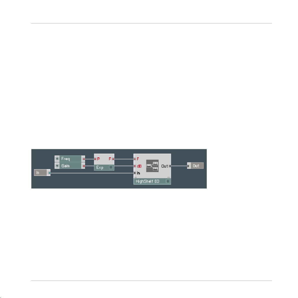
cells exist inside primary-level structures, and they look similar and behave similarly to pri
mary-level built-in modules. Here is an example structure, using a HighShelf EQ core cell,
which differs from the primary-level built-in module version in that it has frequency and
boost controls:
core level and the primary level, respectively. Also when we say
core cells. Core
Inside of core cells are Reaktor Core structures. Those provide an efficient way to imple
ment custom low-level DSP functionality as well as to build larger-scale signal-processing
structures using such functionality. We will take a detailed look at these structures later.
Although one of the main purposes of Reaktor Core is to build low level DSP structures, it
is not limited to that. For users with little DSP programming experience, we have provided
a library of pre-built modules, which you can connect inside core structures, just as you do
with ordinary modules and macros in primary-level structures. We have also provided you
with a library of pre-built core cells, which are immediately available for you to use in pri
mary-level structures.
REAKTOR 5.5 - Core Reference - 16
Page 17
First Steps in Reaktor Core
Using Core Cells
In the future, Native Instruments will put less emphasis on creating new primary-level mod
ules. Instead, we will use our new Reaktor Core technology and provide them in the form of
core cells. For example, you will already find a set of new filters, envelopes, effects, and so on
in the core cell library.
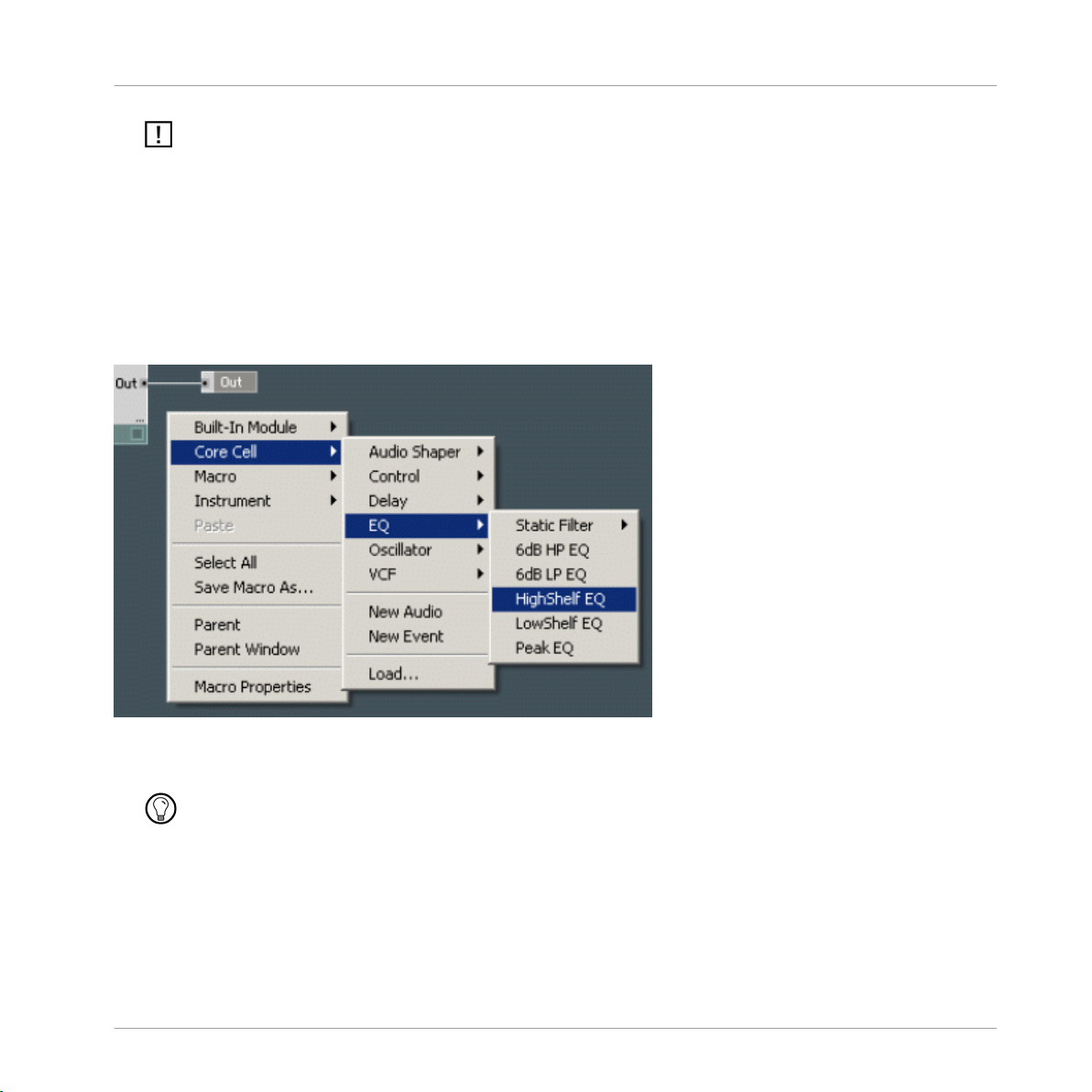
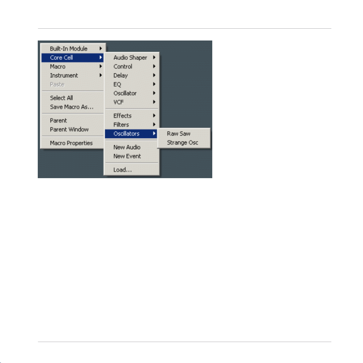
1.2 Using Core Cells
The core cell library can be accessed from primary-level structures by right-clicking on the
background and using the Core Cell submenu:
As you can see, there are all different kinds of core cells; they can be used in the same
way as primary-level built-in modules.
An important limitation of core cells is that you are not allowed to use them inside event
loops. Any event loop occurring through a core cell will be blocked by Reaktor.
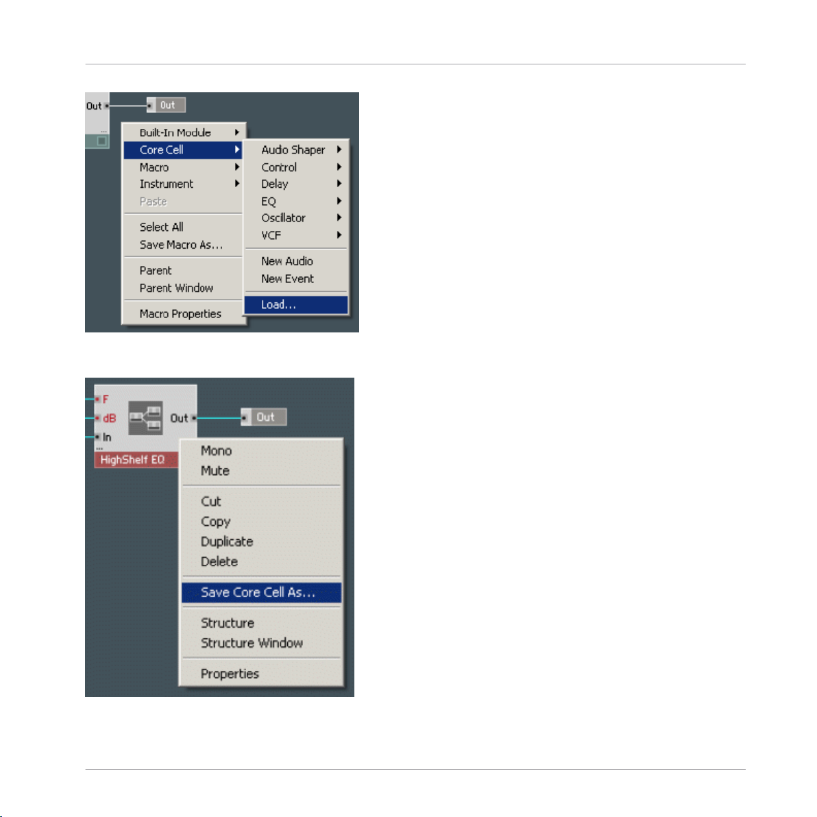
You can also insert core cells that are not in the library. To do that, use the Load… com
mand from the Core Cell menu:
REAKTOR 5.5 - Core Reference - 17
Page 18
First Steps in Reaktor Core
Using Core Cells
You may also want to save core cells you’ve created or modified, so that you can load them
into other structures. To save a core cell, right-click on it and select Save Core Cell As:
REAKTOR 5.5 - Core Reference - 18
Page 19
First Steps in Reaktor Core
Using Core Cells
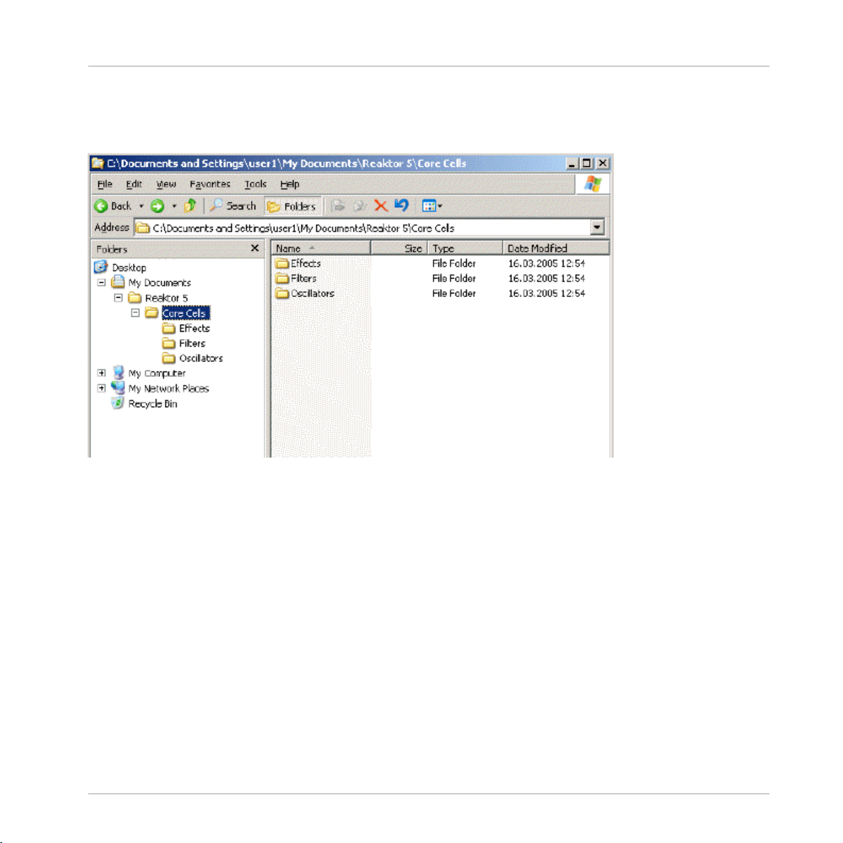
Rather than using the Load… command, you can have your core cells appear in the menu
by putting them into the Core Cells subdirectory of your user library folder. Better still, you
can further organize them into subgroups. Here’s an example:
“My Documents\Reaktor 5” is the user library folder in this example. On your computer
there may be a different path, depending on the choice you’ve made during installation
and any changes you’ve made in Reaktor’s preferences. Inside the user library folder
there’s a folder named “Core Cells”. (Create it manually if it doesn’t exist.)
Inside the Core Cells folder, notice the folder structure consisting of the Effects, Filters,
and Oscillators folders. Inside those folders are core cell files that will be displayed in the
user part of the Core Cell menu:
REAKTOR 5.5 - Core Reference - 19
Page 20
First Steps in Reaktor Core
Using Core Cells in a Real Example
The menu contents are scanned once during Reaktor startup, so after putting new files in
to these folders, you should restart Reaktor.
Empty folders are not displayed in the menu; a folder must contain some files to be dis
played.
Under no circumstances should you put your own files into the system library. The system
library may be changed or even completely replaced when installing updates, in which
case your files will be lost. The user library is the right place for any content that is not
included in the software itself.
1.3
Using Core Cells in a Real Example
Here we are going to take a Reaktor instrument built using only primary-level modules and
modify it by putting in a few core cells. In the Core Tutorial Examples folder in your Reak
tor installation, find the One Osc.ens ensemble and open it. This ensemble consists of on
ly one instrument, which has the internal structure shown:
REAKTOR 5.5 - Core Reference - 20
Page 21

First Steps in Reaktor Core
Using Core Cells in a Real Example
As you can see this is a very simple subtractive synthesizer consisting of one oscillator,
one filter and one envelope. We are going to replace the oscillator with a different, more
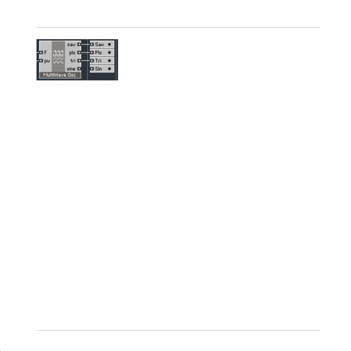
powerful one. Right-click on the background and select Core Cell > Oscillator > MultiWave
Osc:
The most important feature of this oscillator is that it simultaneously provides different an
alog waveforms that are locked in phase. We are going to replace the Sawtooth oscillator
with the MultiWave Osc and use a mix of its waveforms instead of a single sawtooth wave
form. Fortunately, there’s already a mixer macro available from Insert Macro > Classic
Modular > 02-Mixer Amp > Mixer– Simple–Mono:
REAKTOR 5.5 - Core Reference - 21
Page 22
First Steps in Reaktor Core
Using Core Cells in a Real Example
Connect the mixer and the oscillator together and use their combination to replace the
sawtooth oscillator:
Switch to the panel view. Now you can use the four faders of the mixer to vary the wave
form mix.
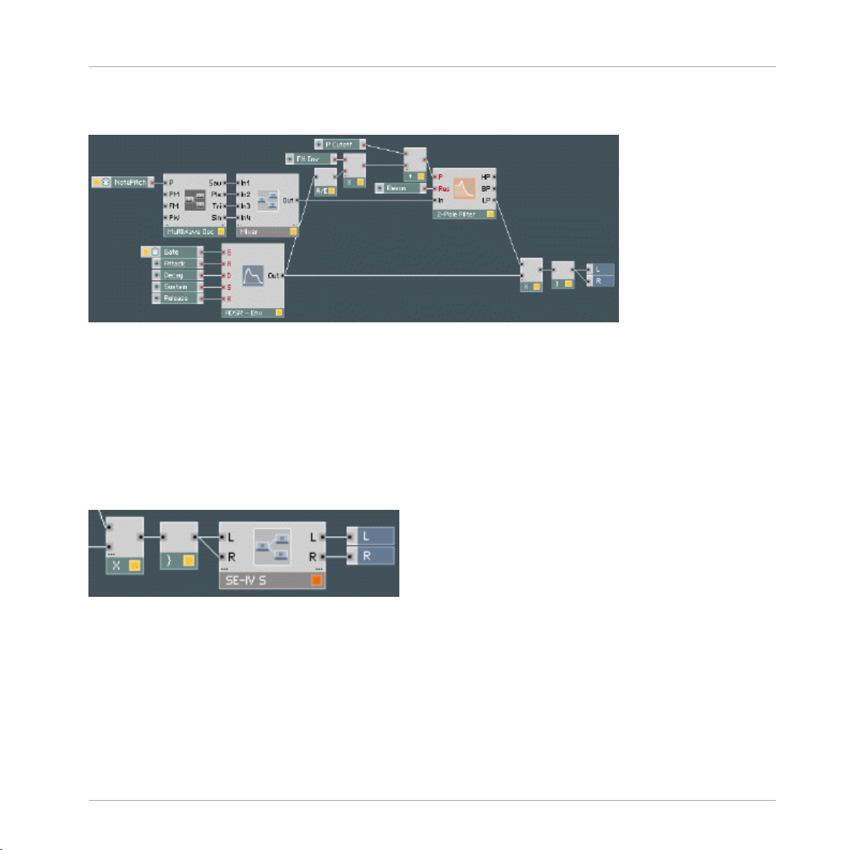
Let’s do one more modification to the instrument and add a Reaktor Core-based chorus ef
fect. We say Reaktor Core based, because although the chorus itself is built as a core cell,
the part containing panel controls for this chorus is still built using the primary-level fea
tures. That’s because at this time Reaktor Core structures cannot have their own control
panels – the panels have to be built on the primary level.
Select Insert Macro > Building Blocks > Effects > SE-IV Chorus and insert it after the
Voice Combiner module:
If you look inside the chorus you can see the chorus core cell and the panel controls:
REAKTOR 5.5 - Core Reference - 22
Page 23
First Steps in Reaktor Core
Basic Editing of Core Cells
1.4 Basic Editing of Core Cells
Now we are about to learn a few things about editing core cells. We are going to start with
something simple: modifying an existing core cell to your particular needs.
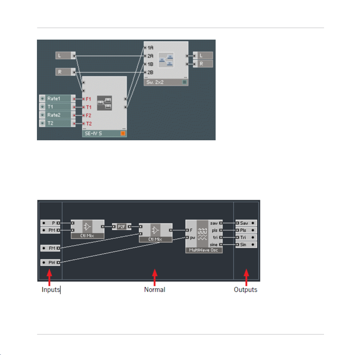
First, double-click the MultiWave Osc to go inside:
REAKTOR 5.5 - Core Reference - 23
Page 24
First Steps in Reaktor Core
Basic Editing of Core Cells
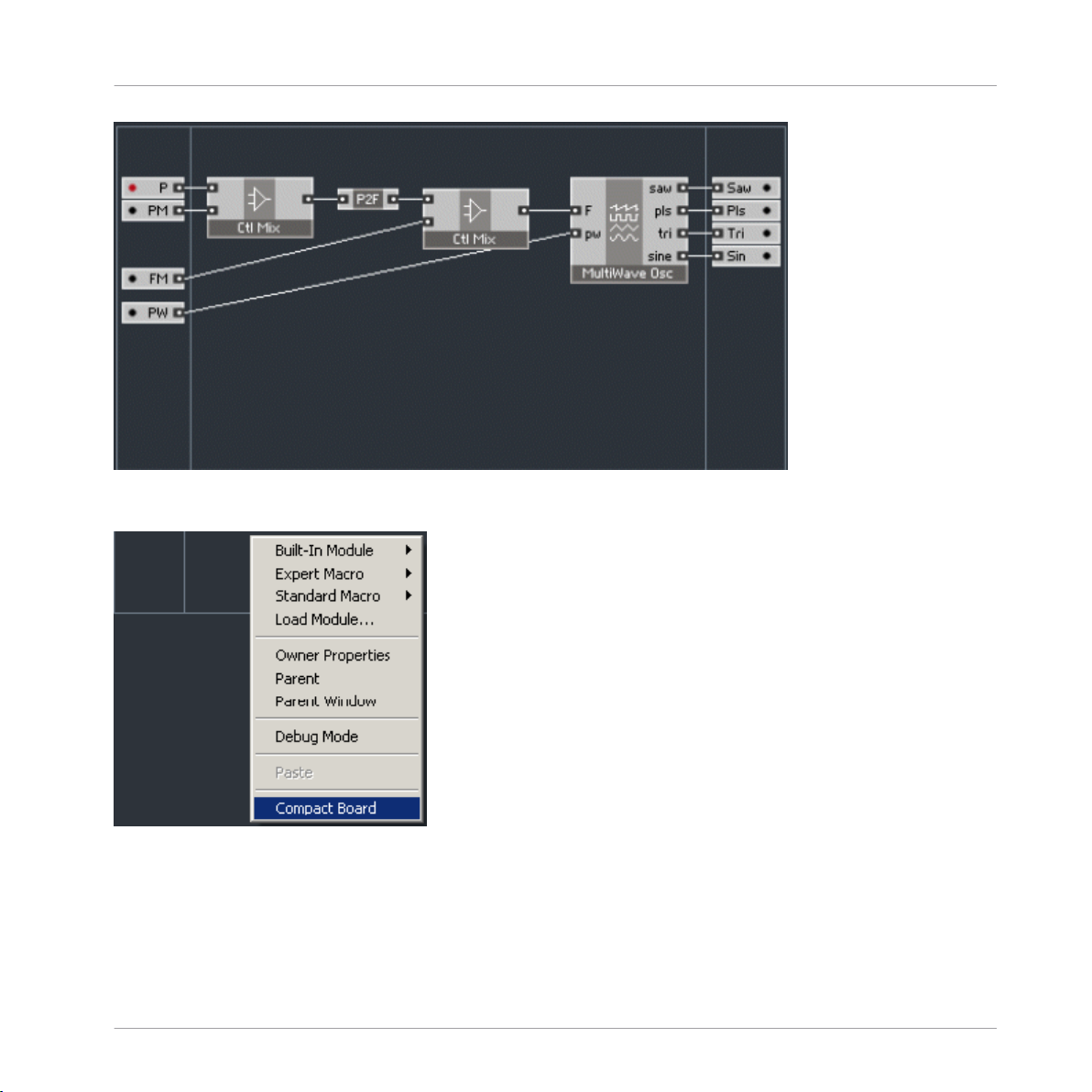
What you see now is a Reaktor Core structure. The three areas separated by vertical lines
are for three different kinds of modules: inputs (on the left), outputs (on the right), and
normal modules (center).
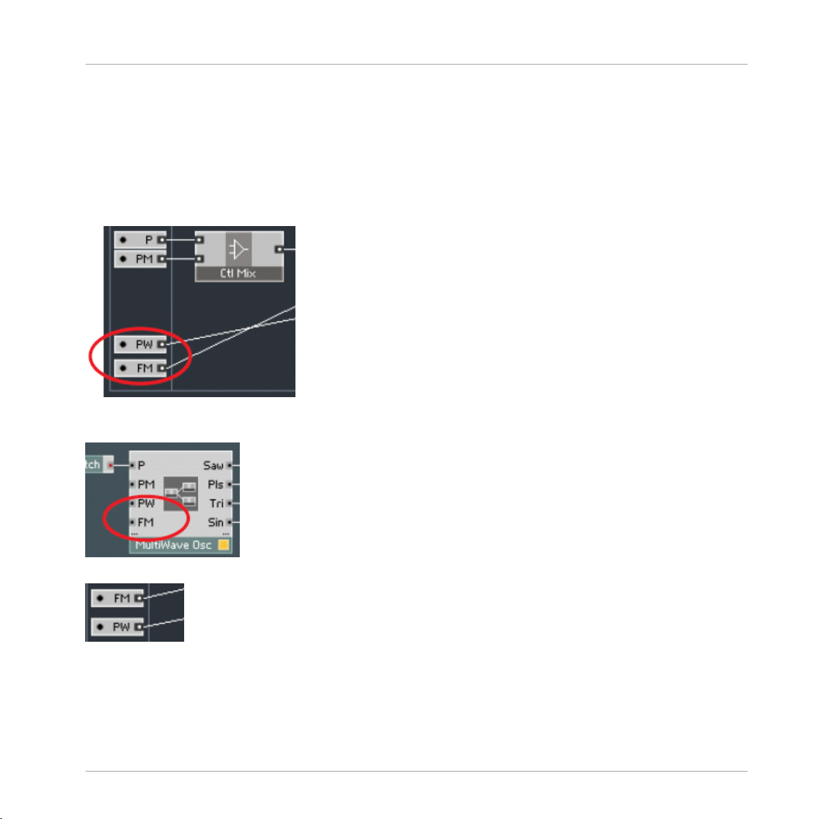
Whereas normal modules can move in all directions, the inputs and outputs can only be
moved vertically, and their relative order matches the order in which they appear outside.
So, you can easily rearrange their outside order by moving them around. Try moving the
FM input below the PW input:
You can double-click the background now to ascend to the outside, primary-level structure
and see the changed port order:
Now go back to the core level and restore the original port order:
As you have probably already noticed, if you move modules around, the three areas of the
core structure automatically grow to accommodate all modules inside them. However, they
do not automatically shrink, which can lead to these areas sometimes becoming unneces
sarily large:
REAKTOR 5.5 - Core Reference - 24
Page 25
First Steps in Reaktor Core
Basic Editing of Core Cells
You can shrink them back by right-clicking on the background and selecting Compact
Board command:
Now that we have learned to move the things around and rearrange the port order of a core
cell, let’s try a few more options.
For a core cell that has audio outputs it’s possible to switch the type of its inputs between
audio and event (a more detailed explanation can be found later in this manual). In the
above example, we used a MultiWave Osc module, all of whose inputs and outputs are au
REAKTOR 5.5 - Core Reference - 25
Page 26
First Steps in Reaktor Core
Basic Editing of Core Cells
dio. However, in this example we don’t really need them as audio, because the only thing
connected to the oscillator is a pitch knob. Wouldn’t it be more CPU efficient to have at
least some of the ports set to event type? The obvious answer is, “yes, it would.” Here’s
how to do that.
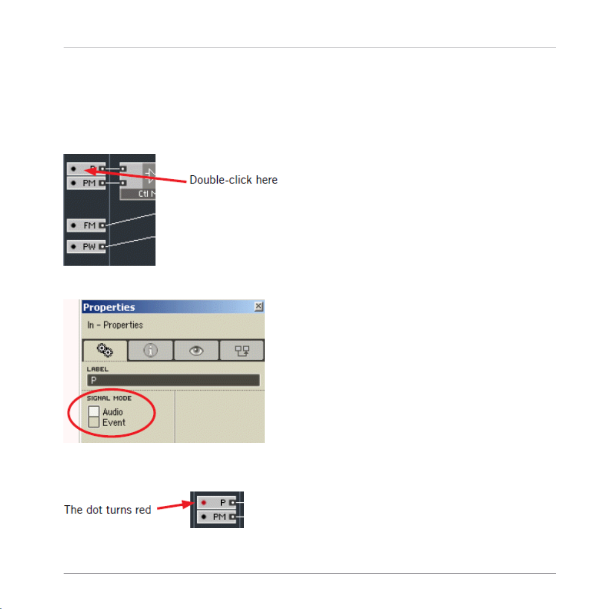
Changing both P and PM inputs to event mode should produce the largest CPU improve
ment. To do that double-click on the P port module to open its properties window:
Switch the properties window to the function page, if necessary, by clicking on the cog
wheel tab. You should now see the Signal Mode property:
Change it to event. Note how the large dot at the left of the input module changes from
black to red indicating that the input is now in event mode (it’s more easily visible after
you deselect the port – just click elsewhere):
REAKTOR 5.5 - Core Reference - 26
Page 27
First Steps in Reaktor Core
Basic Editing of Core Cells
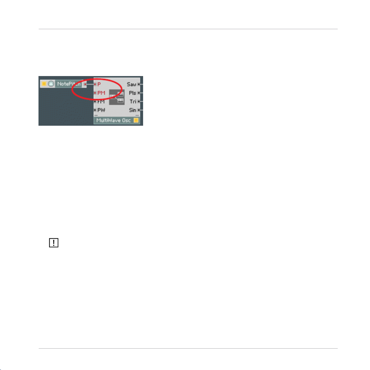
Now click on the PM input to select it, and change it to event mode, too. If you want, you
can change the two remaining inputs to event mode as well. Finally, double-click the
structure background to return to the primary level and observe that the port colors have
changed to red and the CPU usage has gone down.
Sometimes it doesn’t make sense to switch a port from one type to another. For example,
it doesn’t make sense to switch an input that receives a real audio signal (meaning real
audio, not just an audio-rate control signal like an envelope) to an event rate. In some cas
es such switching could even ruin the functionality of the module. Going in the other di
rection, it doesn’t make sense to change an event input that is really event sensitive, such
as an envelope’s event trigger input (for example, gate inputs of Reaktor primary-level en
velopes). If you change such an input to audio, it will no longer work correctly.
In addition to cases in which port-type switching obviously does not make sense there may
be cases in which it does make sense, but in which the modules will not work correctly if
you switch their port types. Such cases are quite special, although they can also result
from mistakes in the implementation or design of the module. Generally, port-type switch
ing should work; hence the following switching rule:
In a well designed core cell, an audio-rate control input can typically be switched to event
mode without any problem. An event input can be switched to audio only if it doesn’t have a
trigger (or other event-sensitive) function.
Another way to save CPU is to disconnect the outputs that you don’t need, thereby deacti
vating unused parts of the Reaktor Core structure. You have to do that from inside the
structure – outside connections do not have any effect on deactivating the core structure
elements.
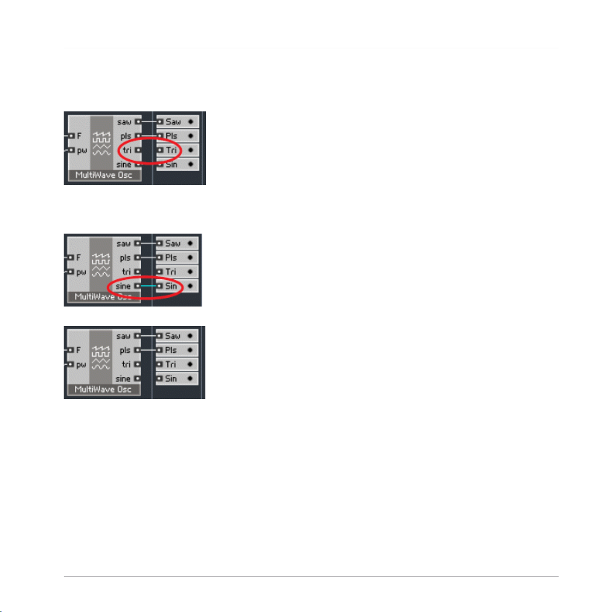
Suppose in our example we decide that we only need the sawtooth and pulse outputs. We
can lower the CPU usage by going inside the MultiWave Osc and disconnecting the unused
outputs. Disconnecting is simple in Reaktor Core, you click on the input port of the con
REAKTOR 5.5 - Core Reference - 27
Page 28
First Steps in Reaktor Core
Basic Editing of Core Cells
nection, drag the mouse to the any empty part of the background and release it. For exam
ple, click on the input port of the Tri output and drag the mouse into empty space on the
background.
There’s another way to delete a connection. Click on the wire between the sine output of
the MultiWave Osc and Sin output of the core cell, so that it gets selected (you can tell
that it’s selected by its blue color):
Now you can press the Delete key to delete the wire:
After you deleted both wires, the CPU meter should go down a little more.
If you change your mind, you can reactivate the outputs by clicking on either the input or
the output that you want to reconnect and dragging the mouse to the other port. For exam
ple, click on the Tri output of the MultiWave Osc and drag to the input of the Tri output
module. The connection is back:
REAKTOR 5.5 - Core Reference - 28
Page 29
First Steps in Reaktor Core
Basic Editing of Core Cells
Of course, numerous fine-tuning adjustments can be made to core cells. You will learn
about many more options as you proceed through this manual.
REAKTOR 5.5 - Core Reference - 29
Page 30
Getting Into Reaktor Core
2 Getting Into Reaktor Core
2.1 Event and Audio Core Cells
Core cells exist in two flavors: Event and Audio. Event core cells can receive only primarylevel event signals at their inputs and produce only primary-level event signals at their out
puts in response to such input events. Audio core cells can receive both event and audio
signals at their inputs but provide only audio outputs:
Flavor Înputs Outputs Clock Src
Event Event Event Disabled
Audio Event/Audio Audio Enabled
Therefore audio cells can implement oscillators, filters, envelopes, effects and other stuff,
while event cells are suitable only for event processing tasks.
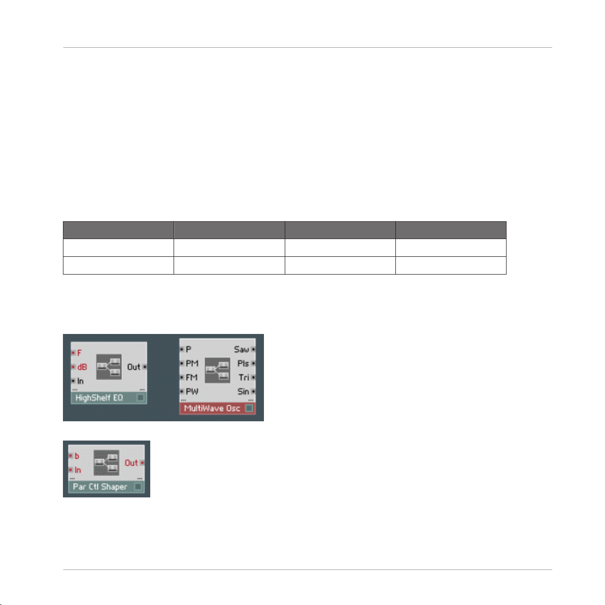
The HighShelf EQ and MultiWave Osc modules that you are already familiar with are ex
amples of audio core cells (you can tell that by the fact that they have audio outputs):
And here is an example of an event core cell:
This module is a parabolic shaper for control signals, which can be used to implement ve
locity curves or LFO signal shaping, for example.
REAKTOR 5.5 - Core Reference - 30
Page 31

Getting Into Reaktor Core
Creating Your First Core Cell
As previously mentioned, event core cells are restricted to event processing tasks. Because
clock sources are disabled inside them (see the table above), they cannot generate their
own events and, therefore, cannot implement modules such as event-rate LFOs and enve
lopes. When you need such modules, we suggest that you take an audio cell and convert
its output to event rate using one of the primary-level audio to event converters:
2.2 Creating Your First Core Cell
You create new core cells by right-clicking on the background in a primary-level structure
and selecting Core Cell > New Audio or, for event cells, Core Cell > New Event:
REAKTOR 5.5 - Core Reference - 31
Page 32

Getting Into Reaktor Core
Creating Your First Core Cell
We are going to build a new core cell from scratch inside the same One Osc.ens you al
ready played with. We will be using the modified version of that ensemble with the new
oscillator and chorus that we built in the last chapter, but if you didn’t save it don’t worry,
you can do the same steps using the original One Osc.ens.
As you can see, in this ensemble we are modulating the filter at the P input, which ac
cepts only event signals. We are not using the FM version of the same filter because it
does not perform as well at higher cutoff frequencies, and because the modulation scale is
linear at an FM input, which generally gives less musical results when modulated by an
envelope. (That phenomenon is typically but incorrectly referred to as “slow envelopes”.):
Because we need to apply the modulation at an event input, we also need to convert the
envelope’s output to an event signal, which we do with an A/E converter. As a result, our
control rate is pretty low. Of course we could have used a converter running at a signifi
cantly higher rate (and eating up significantly more CPU), but what we are going to do in
stead is replace this filter with one which we build as a core cell. Alternatively, we could
have taken an existing filter from the core-cell library, but then we would miss all the fun
of making our first Reaktor Core structure.
We’ll start by creating a new audio core cell. Select Core Cell > New Audio and an empty
audio core cell will appear:
REAKTOR 5.5 - Core Reference - 32
Page 33

Getting Into Reaktor Core
Creating Your First Core Cell
Double-click it to see its structure, which is obviously empty. As you surely remember, the
three areas are meant for input, output, and normal modules:
Attention: we are going to insert our first module into a core structure right now! Rightclick in the normal area to bring up the module creation menu:
REAKTOR 5.5 - Core Reference - 33
Page 34

Getting Into Reaktor Core
Creating Your First Core Cell
The first submenu is called Built-In Module and provides access to the built-in modules of
Reaktor Core, which are generally meant to do really low-level stuff and will be discussed
later.
The second submenu is called Expert Macro and contains macros meant to be used along
side built-in modules for low-level stuff.
The third submenu, called Standard Macro, is the one we want to use:
REAKTOR 5.5 - Core Reference - 34
Page 35

The VCF section could be promising, let’s look inside:
Getting Into Reaktor Core
Creating Your First Core Cell
REAKTOR 5.5 - Core Reference - 35
Page 36

Getting Into Reaktor Core
Creating Your First Core Cell
Let’s try Diode Ladder:
Well, maybe that was not the best idea, because a diode ladder might sound significantly
different from the primary-level filter module we are trying to replace. At minimum, Diode
Ladder is a 4-pole (24dB/octave) filter, and the one we are replacing is a 2-pole filter
(12dB/octave). To delete it there are two options. One is to right-click on the module and
select Delete Module:
The other option is to select the module by clicking on it and pressing the Delete key.
After deleting the Diode Ladder, insert a 2 Pole SV C filter from the same VCF section of
the Standard Macro submenu:
REAKTOR 5.5 - Core Reference - 36
Page 37

Getting Into Reaktor Core
Creating Your First Core Cell
This is a 2-pole, state-variable filter and is similar to the one we are replacing (there are
some differences, but they are quite subtle). What’s important is that we can modulate
this filter at audio rates.
Obviously, we need some inputs and some outputs for our core cell. To be exact we need
only one output – for the LP signal. To create it right-click in the outputs area:
There’s only one kind of module you can create there, so select it. This is what the struc
ture is going to look like:
REAKTOR 5.5 - Core Reference - 37
Page 38

Getting Into Reaktor Core
Creating Your First Core Cell
Double-click the output module to open the Properties window (if it’s not already open).
Type “LP” in the label field:
Now connect the LP output of the filter to the output module:
Now let’s start with the inputs. The first input will be an audio-signal input. Right-click in
the background of the inputs area and select New > In:
The input is automatically created with the right type – it’s an audio input, as you can tell
by the large black dot. Rename this input to “In” in the same way you renamed the output
to “LP”, then connect it to the first input of the filter module:
REAKTOR 5.5 - Core Reference - 38
Page 39

Getting Into Reaktor Core
Creating Your First Core Cell
The second input is a little bit more complicated. As you can see, the second input of the
filter Reaktor Core module is labeled “F”. That means frequency, and if you hold your
mouse over that input for a while (make sure the info button, the cursor with the “i,” is
active), you’ll see the info text, which says “Cutoff frequency (Hz)”:
As we know, the cutoff of our primary-level filter module is controlled by an input labeled
“P”, and as you can see from the info text, the signal uses a semitone scale.
We obviously need to convert from semitones to Hz. We can do that either on the primary
level (using the Expon. (F) module) or inside our Reaktor Core structure. Because we are
learning to build Reaktor Core structures, let’s go for the latter option. Right-click in the
background of the normal area and select Standard Macro > Convert > P2F:
REAKTOR 5.5 - Core Reference - 39
Page 40

Getting Into Reaktor Core
Creating Your First Core Cell
As the name implies (and the info text states), this module converts between P (pitch) and
F (frequency) scales – exactly what we need. So let’s create a second input labeled “P”
and connect it using the P2F module:
That should do it, but wait! In our instrument we have a “P Cutoff” knob defining the base
cutoff of the filter, and to that is added the modulation signal from the envelope, which we
have to convert to an event signal on the primary level in order to feed it into the P input
of the filter. Now that the conversion is no longer necessary, we can remove the A/E mod
ule and plug the audio signal directly into the audio P input of our new filter. Although
this approach is fine, let’s look at another way, just for fun.
We’ll start with our P input in event mode and add another modulation input in audio
mode. (If you remember our discussion about slow envelopes, you will understand why we
decided to call this input “PM”, not “FM”.) We also need to have the modulation input
use the semitones (pitch) scale. That’s exactly how it was done in our original instrument:
we added our envelope signal to the “P Cutoff” signal and plugged the sum into the P in
put.
So first change the P input to the event mode (as described previously) and add another
PM input, which should be in audio mode:
As a user of the Reaktor primary level, you probably expect us to add the two signals to
gether now. In fact, we could do that, but in Reaktor Core the Add is considered a lowlevel module, and using it generally requires some knowledge of fundamental Reaktor Core
low-level working principles. They are not that complex and will be described later in this
text. For now, you don’t need to know them; just use a control signal mixer instead, for
example, Standard Macro > Control > Ctl Mix:
REAKTOR 5.5 - Core Reference - 40
Page 41

Getting Into Reaktor Core
Creating Your First Core Cell
The last input that we need is a resonance input, it doesn’t need to be at audio rate, so
let’s use an event input:
One other thing we need to do is to give our core cell a name. If the Properties window is
already open, click on the background to display the core cell’s properties. If it’s not open,
right-click on the background and select the Owner Properties command:
REAKTOR 5.5 - Core Reference - 41
Page 42

Getting Into Reaktor Core
Creating Your First Core Cell
Now you can type some text into the label field:
Double-click the background to see your result:
REAKTOR 5.5 - Core Reference - 42
Page 43

Getting Into Reaktor Core
Creating Your First Core Cell
Wow, looks nice except that the audio-signal input is at the top of the core cell, while the
primary-level filter module input is on the bottom. We could leave it as is, but it’s easy to
fix, and you already know how. Let’s do it together, and we’ll show you a new feature on
the way.
The first thing to do is go back inside and drag the audio-signal input all the way to the
bottom:
That does the trick, but that diagonal wire over the whole structure doesn’t look particular
ly nice. That’s what we are going to fix now.
Right-click on the output of the In input module and select the Connect to New QuickBus
command:
REAKTOR 5.5 - Core Reference - 43
Page 44

Getting Into Reaktor Core
Creating Your First Core Cell
This is what you should see now:
Also, the Properties window should open to display the properties of the QuickBus you’ve
just created. The most useful QuickBus property is the ability to change its name (other
properties are quite advanced, so don’t touch them for now). You can open the Properties
window later by double-clicking on the QuickBus.
Although you can rename this QuickBus, we believe the current name is perfect, because
it matches the name of the input connected to the QuickBus. (QuickBusses are local to
the given structure, so you don’t need to worry about possible name conflicts when a
neighboring or nested structure is using a QuickBus with the same name.)
The next thing you should do is right-click on the top input of the 2 Pole SV C filter mod
ule and select Connect to QuickBus > In:
In the above menu “In” is the name of the QuickBus you are connecting to. You don’t
want to create a new QuickBus, you want to connect to one that already exists, and that’s
what you’re doing. This is how your structure should look now:
REAKTOR 5.5 - Core Reference - 44
Page 45

Getting Into Reaktor Core
Creating Your First Core Cell
Instead of a nasty looking diagonal wire, we get two nice references, stating that the input
and output are connected by a QuickBus whose name is “In”.
Now we can go back out to the primary level and modify our structure to use the new filter
we’ve just built. The Add and A/E modules can be thrown away. This is our final result:
Takes quite a bit more CPU, doesn’t it? Well, don’t forget that this filter is modulated at
audio rate in pitch scale. If you don’t like it, you can still revert to the old structure or use
the Multi 2-pole FM filter module from the primary level (slow envelopes, remember?), but
we hope that you do like it. Even if you don’t, there are quite a few other filters with new
features that you might like better. And, if you don’t like the new Reaktor Core filters,
there are a whole bunch of other Reaktor Core modules you can try.
REAKTOR 5.5 - Core Reference - 45
Page 46

Getting Into Reaktor Core
Audio and Control Signals
2.3 Audio and Control Signals
Before we proceed we need to take a look at one particular convention used in the Stand
ard Macros of the Reaktor Core library.
bed in terms of several different types of signals: audio, control, event, and logic. We will
explain event and logic signals a little bit later; for now we’ll concentrate on the first two
types.
Audio signals are obviously signals which carry audio information. These include signals
taken at the outputs of oscillators, filters, amplifiers, delays, and so on. Furthermore, mod
ules such as filters, amplifiers, saturators, delays and the like would normally receive an
incoming audio signal to process.
Control signals, on the other hand, do not carry audio, they are used to control other mod
ules. For example, outputs of envelopes and LFOs as well as keyboard pitch and velocity
signals do not carry any sound, but can be used to control a filter’s cutoff or resonance, or
a delay line’s delay time, and so on. Correspondingly, a filter’s cutoff or resonance input
port, or a delay’s time input port are intended to receive control signals.
Here is an example of a Reaktor Core filter module which you already know:
The modules you find in that area are best descri
The upper input of the filter is for the audio signal to be filtered and, therefore, expects an
audio-type signal. The F and Res inputs are obviously control type. The outputs of the fil
ter carry different kinds of filtered audio, so all those signals are also audio type.
A sine oscillator module, on the other hand, has only a single control input (for the fre
quency), and a single audio output:
REAKTOR 5.5 - Core Reference - 46
Page 47

Getting Into Reaktor Core
Audio and Control Signals
And if we take a look at the Rect LFO module, it has two control inputs – for controlling
the frequency and pulse width (the third input is of event type) – and one control output
(because it would be used to control things like filter cutoff or VCA levels, and so on):
Some types of processing, mixing for example, make sense for both audio and control types of
signals. In those cases, you will find versions of such macros dedicated to processing audio
and versions dedicated to processing control signals. For example, there are audio mixers and
control mixers, audio amplifiers and control amplifiers, and so on. Generally it’s not a very
good idea to misuse a module to process signals of types it was not intended for, unless you
really know what you’re doing.
Having said that, quite often it’s possible to use audio signals for control purposes. The most
common example would be to modulate an oscillator’s frequency or a filter’s cutoff by an au
dio signal. That is absolutely OK because you are intending to use an audio signal as a control
signal. We assume that the opposite case, in which you really mean to use a control signal as
an audio signal, would be pretty rare.
The separation between audio, control, event, and logic signals is not to be confused with
event/audio separation on the Reaktor primary level. The primary-level event/audio classifi
cation refers to speed of processing, audio signals being processed faster and requiring
more CPU. Also as you probably know, primary-level event signals have different propaga
tion rules than audio signals. The difference between audio, control, and event signals in
Reaktor Core terminology is purely semantic, defining the meaning of the signal rather
than the type of processing. There is not a one-to-one relationship between primary-level
event/audio and Reaktor Core audio/control/event/logic terms, but we can still try to ex
plain their relationship:
▪ A primary-level audio signal normally corresponds to either a Reaktor Core audio sig
nal (for example, an output of an oscillator or an audio filter) or a Reaktor Core con
trol signal (for example, an output of an envelope).
▪ A primary-level event signal is typically a control signal in terms of Reaktor Core. An
example of such signal would be an output of an LFO, a knob, or a MIDI pitch or ve
locity source.
REAKTOR 5.5 - Core Reference - 47
Page 48

Getting Into Reaktor Core
Audio and Control Signals
▪ Sometimes a primary-level event signal corresponds to a Reaktor Core event signal.
The most typical example of that is a MIDI gate (Reaktor Core event signals will be
described later, as we promised).
▪ Sometimes a primary event signal resembles a Reaktor Core logic signal; however,
they are not fully compatible, and there must be explicit conversion between them (a
topic that also will be covered later). Examples include signals processed by Logic
AND or similar primary-level modules.
It’s important to understand that when you select the type for a core-cell input port, you are
choosing between the primary-level event and audio signals, not between Reaktor Core event
and audio signals. The core-cell ports are the place where both worlds meet, and therefore,
they use a bit of the primary-level terminology.
We are going to learn a little bit more about this concept while trying to build a tape-echoeffect emulation. We will start by building a simple digital echo, then enhance it to emu
late some features of a tape echo.
Start by creating an empty audio core cell; then go inside and set its name to “Echo”.
The first module we are going to put into the structure is a delay module. We will pick a 4point interpolating delay, because it has better quality than a 2-point delay, and a noninterpolating delay would not be suitable for our tape emulation: Standard Macro > Delay
> Delay 4p:
We obviously need an audio input and an audio output for our delay core cell. We will use
a QuickBus connection for the input and a normal connection for the output:
REAKTOR 5.5 - Core Reference - 48
Page 49

Getting Into Reaktor Core
Audio and Control Signals
We also need an event input for controlling the delay time. One thing to be aware of here
is that, on the primary level, the delay time is usually expressed in milliseconds, while Re
aktor Core library delay macros expect it to be in seconds. No problem, there is a conver
sion module available for that. Standard Macro > Convert > ms2sec:
So far, we only have a single echo, and it would also be nice to hear the original signal,
not just the echo. To get the original signal at the output we need to mix it with the de
layed signal. Because we are mixing audio signals here, we need to use an audio mixer
(you may remember we used a control mixer to mix control signals when we were building
a filter core cell). Even better, we can use a particular audio mixer type that is specifically
designed to crossfade between two signals: Standard Macro > Audio Mix-Amp > XFade
(par):
Here “(par)” stands for parabolic, which produces a more natural sounding crossfade than
a linear crossfade. We will connect the control (x) input of the crossfade to a new event
input to control the mix between the dry (unprocessed) and wet (delayed) signals. When
the control signal is 0 we will hear only the original signal, and when it’s 1, we will hear
only the delayed signal:
REAKTOR 5.5 - Core Reference - 49
Page 50

Getting Into Reaktor Core
Audio and Control Signals
Now we can hear the original signal and the echo, but there’s still only one echo. To have
multiple echoes we need to feed a fraction of the delayed signal back to the delay input.
First we need to attenuate the delayed signal. Following the same guidelines, use an audio
amplifier to attenuate an audio signal by choosing Standard Macro > Audio Mix-Amp >
Amount.
We use the Amount amp because we want to control the amount of the signal that is fed
back. Also, this amplifier will allow us to invert the signal by using negative amount set
tings. In contrast, for example Amp (dB), which would be quite suitable to control the sig
nal volume, is not very good here because it doesn’t allow us to invert signals. We connect
the amplitude control input of the amplifier to an event input controlling the feedback
amount:
REAKTOR 5.5 - Core Reference - 50
Page 51

Getting Into Reaktor Core
Audio and Control Signals
The reasonable feedback amount range is something like [-0.9..0.9] here. When you try out
this delay, be careful with the feedback amount, because you can easily reach excessive sig
nal levels (there is no saturation in our circuitry yet). We could have embedded a safety feed
back amount clipper into our delay core cell, but because we are going to have saturation
there a little bit later, we didn’t think that was necessary. Without it, you will be able to ex
periment with high feedback levels and hear the delay saturating.
We need to mix the feedback signal with the input signal. An audio mixer (Standard Macro
> Audio Mix-Amp > Audio Mix) is a natural choice
You may wonder what happened to the upper input of the Amount module above, which
now shows a large orange “Z”:
Actually, depending on the version of the software and other conditions, the Z sign could
appear at some other input in the structure, but don’t worry you too much about it. The Z
sign indicates that a digital feedback has occurred in the structure, and it is meant for ad
vanced structure design, where such information can be an important hint for the struc
ture designer.
For simple structures like the one above, one normally needn’t worry about the Z sign; its
presence just shows that there will be a 1-sample delay (about 0.02ms at 44.1kHz, even
less at higher sampling rates) at that point in the structure. We assume you won’t notice if
your delay time is 0.02ms off the specified value.
REAKTOR 5.5 - Core Reference - 51
Page 52

Getting Into Reaktor Core
Audio and Control Signals
Let’s get back to our structure, which now can produce a series of decaying echoes. It is
already a decent digital echo, but we want to show you a feature of the library that you can
use as a trick to make your structure smaller.
Among the audio amplifiers are amplifiers called “Chain”. These amplifiers are capable of
amplifying a given signal and mixing it with another, chained signal. One of them is the
Audio Mix-Amp > Chain(amount) amplifier, which works similarly to the Amount amplifier
except that it also does chained mixing:
The signal at the second input of this module will be attenuated according to the amount
given at the A input and mixed with the signal at the chain (>>) input. The signal at the
chain input is not attenuated. Such amplifiers can be used to build mixing chains, where
the >> port connections constitute a mixing bus:
case we don’t need a mixing bus, but we can use this module to replace both our Audio
Mix and Amount modules. The fed back signal will be attenuated by the amount specified
by the Fbk input and mixed to the input signal exactly as it was before:
Congratulations, you have built a simple digital-echo effect. The next step is to add some
tape feel to it.
REAKTOR 5.5 - Core Reference - 52
Page 53

Getting Into Reaktor Core
Building Your First Reaktor Core Macros
2.4 Building Your First Reaktor Core Macros
In the echo effect we just built, we used a Delay 4p macro from the library, which gives us
a reasonably high-quality digital delay. But, high-quality or not, it still sounds too digital.
We will make it sound warmer by adding two features found in tape delays: saturation and
flutter.
Let’s start by deleting the delay macro from the structure and creating an empty macro in
stead. Right-click on the background as select Built-In Module > Macro:
Double-click it to dive inside. You will see an empty structure, similar to the one you are
diving from:
It also works similarly, but there are some important differences because the previous one
was a structure of a Reaktor Core cell, whereas this one is an internal structure of a Reak
tor Core macro.
These differences have to do with the available input and output modules,
which are different:
REAKTOR 5.5 - Core Reference - 53
Page 54

Getting Into Reaktor Core
Building Your First Reaktor Core Macros
The Latch and Bool C types of ports will be explained much later in this manual and are
used for advanced stuff. We are interested now only in the first type, which is called “Out”
(or “In” for inputs). It’s a general type of port that can accept audio-, control-, event-, and
logic-type signals. In fact, the port doesn’t care whether it’s audio, control, event, or logic;
the difference is important only for you as a user, because it describes how the signal is to
be used; for Reaktor Core they are all the same. There is also no difference between audio/
event inputs/outputs as on the previous structure level, because we don’t have Reaktor pri
mary-level signals on the outside any longer, it is pure Reaktor Core now. The first thing
we are going to do is
name the macro, which is done in the same way as for core cells, by
right-clicking on the background, selecting Owner Properties, and typing in the name:
REAKTOR 5.5 - Core Reference - 54
Page 55

Getting Into Reaktor Core
Building Your First Reaktor Core Macros
The remaining properties of the macro control various aspects of its appearance and its
signal processing.
While you are free to experiment with remaining properties as you see fit, we strongly advise
against turning the Solid parameter off. We also advise changing the FP Precision sparingly.
The meaning of these parameters will be described in the advanced topics of this manual.
The next thing is to create a set of inputs and outputs for our Tape Delay macro:
The upper input will receive the audio input, and the lower will receive the time parame
ter. You may have noticed extra ports on the left side of the input modules; we will explain
them a little bit later.
As the central part of our macro we will use the same Delay 4p module:
REAKTOR 5.5 - Core Reference - 55
Page 56

Getting Into Reaktor Core
Building Your First Reaktor Core Macros
A simple emulation of the saturation effect can be done easily by connecting a saturator
module before the delay. Saturator is a kind of signal shaper, so we will look for it among
the audio shapers (because it is an audio saturator). Standard Macro > Audio Shaper >
Parabol Sat:
The input signal will now
be saturated within the range of –1..+1. Actually, the range is controlled by the L input of
the saturator module, if it is disconnected it defaults to 1. That might be surprising to you
because you are probably used to disconnected inputs being treated as if they receive no
signal, or put differently, a zero signal. Well, this is not exactly the case in Reaktor Core
structures—modules can specify special treatment for disconnected inputs. The saturator,
for example, specifies the L input to have a default value of 1.
Now we are going to learn to do exactly the same, by specifying a new default value for our
T input. Let’s say that if our T input is disconnected we would like it to be treated as if the
input value was 0.25 sec. Very easy. Right-click on the port on the left of the T input mod
ule and select
Connect to New QuickConst. This is what you should see:
In addition, you should have the properties window displaying the properties of the con
stant (if it shows a different page, press the cog wheel tab):
REAKTOR 5.5 - Core Reference - 56
Page 57

In the value field type a new value of 0.25:
Getting Into Reaktor Core
Building Your First Reaktor Core Macros
This is how the QuickConst should look now in the structure:
Let’s explain what we have just done. The port on the left side of the input module speci
fies a so-called default signal. That means that if the input is not connected (on the out
side of the macro), the default signal will be taken as the input source. In our case, if the
T input of the Tape Delay macro is not connected on the outside, it will behave as if you
have connected a constant value of 0.25 to it.
Of course, a connection to the QuickConst is not the only possible connection for the de
fault signal input. You can connect it to any other module in the structure, including other
input modules.
REAKTOR 5.5 - Core Reference - 57
Page 58

Getting Into Reaktor Core
Building Your First Reaktor Core Macros
Now that we have saturation and a default value for the T input, let’s emulate a tape flut
ter effect. A simple way to do that is to modulate the delay time with an LFO. You could
experiment with different LFO shapes for better flutter effect, but for now, just take one
from the library: Standard Macro > LFO > Par LFO:
This is a parabolic LFO, which produces a signal similar in shape to a sine, but uses less
CPU. Its F input must receive a signal specifying the oscillation rate. We can use a Quick
Const again here. A rate of 4 Hz seems reasonable so we can try that:
The Rst input is used for restarting the LFO; we won’t need it for now.
Now we need to specify a modulation amount by scaling the output of the LFO. Currently
the LFO output signal varies in the range –1 .. 1 and that is way too much. Because we
are dealing with control signals here, we are going to use a control amount module, which
is similar to the Amount amplifier we used for audio. Standard Macro > Control > Ctl
Amount:
A modulation amplitude of 0.0002 should do fine, so we scale the signal to that amount:
Ultimately, we can mix the two control signals (one from the T input and one from the Ctl
Amount module) and feed them into the T input of the delay module. The already familiar
Ctl Mix module can be used for that:
REAKTOR 5.5 - Core Reference - 58
Page 59

Getting Into Reaktor Core
Building Your First Reaktor Core Macros
Actually, we have a Chain type of control mixer that is similar to the mixer we have for au
dio signals. We could use it to replace the Ctl Amount and the Ctl Mix modules in the
same way we did earlier in the audio path. Standard Macro > Control > Ctl Chain:
As one last touch for our macro, we are going to change the buffer size for our delay,
which defines the maximum possible delay time. If you hold your mouse cursor over the
Delay 4p macro (provided the cursor info button for info popus on rollover is active), you
can read in the hint text that the default buffer size corresponds to 1 sec of delay at
44.1kHz:
REAKTOR 5.5 - Core Reference - 59
Page 60

Getting Into Reaktor Core
Building Your First Reaktor Core Macros
Let’s increase the amount to 5 seconds (44,100*5 = 220,500 samples). Because each
sample requires 4 bytes, we need 220,500*4 = 882,000 bytes, which is almost 1MB).
Double-click on the Delay 4p macro:
The module on the left is the delay buffer module. Double-click it (or right-click and select
Show Properties) to edit its properties. Select the cog wheel tab and you should see the
Size property. Change it to 220,500 samples:
As we have seen, a delay buffer for 5 seconds of audio takes almost 1MB of memory, so be
careful when changing delay buffers. That’s most important when the delays are used in poly
phonic areas of the structure, because the size of the buffer will be multiplied by the number
of voices.
Now we can go outside the Delay 4p macro and then outside the Tape Delay macro we’ve
just created (double-click the background) and make the outside connections:
REAKTOR 5.5 - Core Reference - 60
Page 61

Getting Into Reaktor Core
Using Audio as Control Signal
If you haven’t done so yet, try out the echo module now. Here’s a Reaktor primary-level
test structure, as simple as possible (note that the Echo module is set to mono):
You might want to enhance it in various ways, for example, by providing knobs controlling
the echo parameters, by using a real synthesizer as a signal source, and so on.
2.5 Using Audio as Control Signal
We have mentioned above that it is possible to use an audio signal as a control signal. As
an example of that, we are going to create a Reaktor Core cell implementing a pair of os
cillators, in which one modulates the other. Start by creating two multiwave oscillators:
REAKTOR 5.5 - Core Reference - 61
Page 62

Getting Into Reaktor Core
Using Audio as Control Signal
We need pitch control for both of the oscillators, and we are going to listen to the output
of the second one, so let’s create the necessary inputs and outputs:
Now we want to take the output of the left oscillator and use it to modulate the frequency
of the right oscillator:
The Mod input controls the modulation amount.
Notice that we are mixing the modulation signal with the P1 input after a P2F converter so
the modulation will take place in frequency scale. (It’s also possible to modulate in pitch
scale.)
It’s also a good idea to scale the modulation amount according to the base oscillation fre
quency:
REAKTOR 5.5 - Core Reference - 62
Page 63

Getting Into Reaktor Core
If you analyze the above structure from the point of view of control and audio signals you
will notice that all of the signals in the structure except the outputs of the oscillators are
control signals. The outputs of both oscillators are obviously audio signals. Notice, howev
er, that we are misusing the output of the left oscillator as control signal at the point at
which we feed it into the Ctl Chain mixer.
2.6 Event Signals
As we said earlier, there are different meanings of the term event signal. You should al
ready be familiar with the idea of Reaktor primary-level event signals. There are several
ways of using a primary-level event signal. One is as a control signal (for example, LFO
output, knob output, and so on), because it uses less CPU than a primary-level audio sig
nal. In that case, you probably could achieve the same effect with an audio signal. But,
there are also cases in which an audio signal won’t work for control, for instance, when you
are interested in both the value of the signal and when the value is sent. A primary-level
envelope-gate signal is an example of that, because the envelope will be triggered when
the event arrives at the gate input.
When we were talking about audio, control, event, and logic signals in Reaktor Core we
were not really talking about different types of signals (technically they are all the same in
Reaktor Core). Rather we are talking about different ways of using a signal. As we now
know, a Reaktor primary-level event signal can be used as a control, event, or even logic
signal, and as we’ve seen from an earlier example, a Reaktor primary-level audio signal
can be used as audio or control.
We have already learned to feed primary-level event signals into Reaktor Core structures
and use them there as control signals. Event-mode inputs for an audio core cell imple
menting a filter that we built earlier is a good example of that. There are also cases in
which you would use an event core cell to process some primary-level event signals used
as control signals. Here’s an example in which an event core cell wraps a control shaper
core macro:
Event Signals
REAKTOR 5.5 - Core Reference - 63
Page 64

Getting Into Reaktor Core
The control shaper receives an event rate control signal from the primary level (for exam
ple, a MIDI velocity signal, or a primary-level LFO signal), bends it according to the Shp
parameter, and forwards the result to the output.
An important restriction of event core cells, which we mentioned earlier, is that all clock sour
ces are disabled inside them. That means that not only oscillators and filters, but also enve
lopes and LFOs do not work inside event core cells. Those modules are restricted to receiving
events from the primary level of Reaktor, processing them, and sending them back to the pri
mary level, as in the above example.
Event Signals
Alternatively, signals derived from primary-level events can be used as true event signals
inside Reaktor Core structures. Let’s take a look at a couple of simple cases of using
events inside Reaktor Core.
The first case is using an envelope in a core structure. As you can guess from the disa
bled-clock restriction on event core cells, this has to be an audio core cell. So, create a
new audio core cell and choose Standard Macro > Envelope > ADSR:
REAKTOR 5.5 - Core Reference - 64
Page 65

Getting Into Reaktor Core
The top input of the envelope is a gate input, which works similarly to the gate inputs of
primary-level envelopes—that is, it opens or closes the envelope in response to incoming
events. For that we create an event input for our core cell:
This input will translate the incoming primary-level gate events into the core events.
Now let’s take a look at the A, D, S, R inputs. The S (sustain level) input works similarly to
the primary level; it expects the incoming signal to be in the 0 to 1 range:
Event Signals
The A, D, R inputs are different, however. Unlike primary-level envelopes they expect time
to be specified in seconds:
That can be solved by using a Standard Macro > Convert > logT2sec, which converts the
primary-level envelope times to seconds:
REAKTOR 5.5 - Core Reference - 65
Page 66

Getting Into Reaktor Core
Although all inputs in the above structure are in event mode, the first input produces an
event signal, whereas the others produce control signals.
Our envelope still has two unconnected ports. The GS port sets the gate sensitivity
amount. At 0 the envelope completely ignores the gate level and is always at full ampli
tude. At 1 the gate level has maximum effect, as on the Reaktor primary level. We can
control this amount from the outside by adding another input:
Event Signals
The RM port specifies the retrigger mode for the envelope:
REAKTOR 5.5 - Core Reference - 66
Page 67

Getting Into Reaktor Core
The look of this port is different from the others because it expects integer values, but that
doesn’t mean we cannot connect non-integer signals to this port. We can simply use an
other event input, and the incoming values will be rounded to the nearest integer:
Event Signals
Now let’s take a look at another example using a true event signal:
REAKTOR 5.5 - Core Reference - 67
Page 68

Getting Into Reaktor Core
The above structure implements a kind of pitch modulation effect. The effect is produced
by a delay whose time varies in the range 250±100 ms. The rate of variation is deter
mined by the Rate input, which controls the rate of the modulating LFO (the value is in
Hz)—that is a pure control signal. The Rst input is a true event signal and can be used for
restarting the LFO. The incoming value specifies the restart phase, where 0 would restart
the LFO at the beginning of the cycle, 0.5 in the middle, and 1 in the end. You can try it
out by connecting a button to send a specific value to this input.
2.7 Logic Signals
Now that we have learned about control and event signals, it’s time to learn about another
way of using signals in Reaktor Core, that would be as logic signals. Here’s an example of
a module that processes logic signals:
Logic Signals
Notice that the ports of this module are integer type, just as was the RM input of the enve
lope. That is because, generally, logic signals carry only integer values; more precisely,
they carry only values of 0 and 1.
For logic signals, a value of 1 stands for true, and a value of 0 stands for false. The mean
ing of “true” and “false” is, of course, up to the user; for instance, it could mean (as in
the example here) whether a particular gate is open (true) or closed (false):
REAKTOR 5.5 - Core Reference - 68
Page 69

Getting Into Reaktor Core
Here a Gate2L macro checks the incoming gate signal and produces a true (1) output if
the gate is open and false (0) output if the gate is closed.
We can use logic signals to do logical processing. For example, here we’ve built a gate pro
cessor that applies a regular clocked gate over a MIDI gate:
The Gate2L, AND, and L2Gate modules are logic modules and can be found in Standard
Macro > Logic menu. The Gate LFO is a macro, which we’ve built for this processor; it
generates an opening and closing gate signal at regular intervals.
The input gate and the output of the LFO are connected to Gate2L converters, which con
vert the gate signals to logic signals, transforming open gates into true and closed gates
into false. The AND module outputs a true signal only if both gates are in the open state at
the same time. In other words the output of the AND module is true if and only if the user
holds a key and at the same time the LFO outputs an open gate. That means that, as long
as the user holds a key, there will be alternating true and false values at the output of the
AND module, the speed of the alternation defined by the LFO rate. The output of the AND
module is converted back to a gate signal, whose amplitude is taken from the gate input,
thereby leaving the gate level unchanged. Here is the structure for our Gate LFO macro:
Logic Signals
The F input defines the rate of the gate repetitions, and the W input defines the duration
of open gates (at 0 they are 50% of the gate period, at –1 it’s 0%, and at 1 it’s 100%).
The Rst input restarts the LFO in response to incoming events (hence the LFO is restarted
each time there’s a gate event at the main gate input).
REAKTOR 5.5 - Core Reference - 69
Page 70

Getting Into Reaktor Core
The module connected to the Rst input of the Rect LFO is called Value and can be found
in Standard Macro > Event Processing. It ensures the LFO is restarted at zero phase by
replacing the values of all incoming events by the value at its lower input, which is zero.
The LFO output is converted into a gate signal by using a Ctl2Gate converter, also found in
Standard Macro >Event Processing.
Remember, LFOs do not work inside event core cells. If you want to try out this structure,
you’ll need to use an audio core cell.
Logic Signals
REAKTOR 5.5 - Core Reference - 70
Page 71

Reaktor Core Fundamentals: The Core Signal Model
3 Reaktor Core Fundamentals: The Core Signal Model
3.1 Values
Most of the outputs of Reaktor Core modules produce values. (Producing a value means
that at any moment in time there is a value associated with the output.) The values are
available to all modules whose inputs are connected to those outputs.
In the following example an adder module gets values 2 and 3 from the two modules
whose outputs are connected to its inputs, and it produces a value of 5 at its output.
If you want to draw an analogy to the hardware world you can think of values as signal levels
(voltages), especially with relatively large-scale modules such as oscillators, filters, envelopes,
and so on. However, values are not limited to those kinds of processing—they are just values
and can be used to implement any processing algorithm, not just voltage-modeling algorithms.
3.2 Events
Time is not continuous in the digital world; it is discrete. Probably the most familiar exam
ple of this is that a digitally stored recording doesn’t store the full information about an
audio signal, which is continuously changing over time, but rather stores only information
about the signal level at regularly spaced points in time. The number of points per second
bears the famous name of sampling rate.
Here is a picture of a continuous signal:
REAKTOR 5.5 - Core Reference - 71
Page 72

and its digital representation:
Reaktor Core Fundamentals: The Core Signal Model
Events
Because we are in the digital world, the outputs of our modules cannot change values con
tinuously. On the other hand, we don’t have to limit ourselves to changing values at regu
larly spaced points in time. For one thing, we do not have to maintain a particular sam
pling rate all over our structures. For another thing, in certain areas of our structures we do
not even have to maintain any sampling rate at all; that is, our changes do not have to
happen at regular intervals.
For example, at time zero the output of our adder could have a value of 5. The first change
could occur at time 1 ms (one millisecond). The second change could occur at 4 ms. The
third at 6 ms:
REAKTOR 5.5 - Core Reference - 72
Page 73

Reaktor Core Fundamentals: The Core Signal Model
In the picture above we can see changes of the output of our adder occurring during the
time from 0 to 7 ms. At the moment in time that the output changes its value, it generates
an event. An event means that the output reports a change of its state, meaning that it has
got a new value.
In the following example, the upper left module has changed its output value from 2 to 4,
generating an event. In response, the adder module will change its output value and gen
erate an event at its output, too.
Events
Alternatively, the upper left module could have generated a new event with the same value
as the old one. The adder would have still responded by generating a new event, but this
time, without changing its output value.
REAKTOR 5.5 - Core Reference - 73
Page 74

Reaktor Core Fundamentals: The Core Signal Model
Simultaneous Events
The new value appearing at the output is not required to be different from the old one. Howev
er, the only way an output can change its value is by generating an event.
As you have seen from the previous examples, an event occurring at an output of some
module will be sensed by downstream modules, which would in turn produce further
events (remember the adder producing an output event in response to an incoming event).
Those new events would be sensed by the modules connected to the corresponding out
puts and propagated further downstream, until the propagation stops for one of the rea
sons discussed later in this text.
Events in Reaktor Core are not the same as events on the Reaktor primary level. They behave
according to different rules, which will be explained below.
3.3 Simultaneous Events
Consider the situation in which the two modules on the left side in the previous examples
simultaneously produce an event.
REAKTOR 5.5 - Core Reference - 74
Page 75

Reaktor Core Fundamentals: The Core Signal Model
Simultaneous Events
This is one of the key features of the Reaktor Core event model—events can occur simulta
neously at several places. In that situation, the events originating at both the left-side
modules will arrive at the inputs of the adder simultaneously, and most importantly, the
adder will produce exactly one output event in response.
That is not the same as on the Reaktor primary level, where events cannot happen simultane
ously, and the Add module (in event mode) would produce two output events in such a situa
tion.
Of course, in reality, the events are not produced simultaneously by the upper-left and the
lower-left modules, because both modules are being processed by the same CPU, and the
CPU can process only one module at a time. But, what is important for us, is that these
events are logically simultaneous, that is they are treated as simultaneous by the modules
receiving them.
Here is another example of simultaneous event propagation:
In the example above, the leftmost module is sending an event, changing its output value
from 2 to 3. The event is sent simultaneously to both the inverter (–x) and the multiplier
(*) modules. In response to the incoming event the inverter will produce a new output val
ue –3. It is important to notice that although the output event of the inverter was pro
duced in response to the event sent by the leftmost module, and as such should happen
later than the incoming event, both events are still logically simultaneous. That means
they simultaneously arrive at the inputs of the multiplier, and the multiplier again produ
ces only one output event, with a value of –9.
Again, on the primary level you would have had two events at the output of the Event Mult
module. It is also not defined whether the event at the output of the leftmost module would
have been sent first to the inverter or to the multiplier (although that is irrelevant for the given
structure).
REAKTOR 5.5 - Core Reference - 75
Page 76

Reaktor Core Fundamentals: The Core Signal Model
Processing Order
In general you can use the following rule to figure out whether two events are simultane
ous or not:
All events originating from (sent in response to) the same event are simultaneous. All events
originating from an arbitrary number of simultaneous events (occurring at different outputs,
but known to be simultaneous) are also simultaneous.
The last example shows the benefit of having simultaneous events. In that case, we elimi
nate the redundant processing of the second event by the multiplier, which would have
taken extra CPU time. In longer structures, in the absence of simultaneous events, the
number of events can grow uncontrollably unless the structure designer pays particular at
tention to keeping the number of duplicate events low.
In addition to saving CPU time, the concept of simultaneity leads to important differences
in one’s approach to structure construction, especially for the structures implementing
low-level DSP algorithms. You will become more familiar with these differences as you
start constructing your own structures.
3.4 Processing Order
As you have seen from the previous examples, when a module sends an event, the down
stream modules respond to that event. From that, one might conclude that, despite pro
ducing logically simultaneous events, the modules are definitely not processed simultane
ously. One might further conclude that, for a given connection, it would be reasonable to
process the upstream module of the connection before the downstream module of the con
nection. All those conclusions are, in fact, correct.
The general rule of processing order of the modules is:
If two connected modules are processing logically simultaneous events, then the upstream
module will be processed first. If the events are not simultaneous, then of course, the order of
processing for the modules is the order of the processed events.
From the above rule it follows that as long as there is a one-direction connection path (al
ways upstream or always downstream) between two modules, then there is a defined proc
essing order for these two modules: the upstream module is processed first.
REAKTOR 5.5 - Core Reference - 76
Page 77

Reaktor Core Fundamentals: The Core Signal Model
If there is no one-direction connection path between two modules, their processing order rela
tive to each other is undefined for logically simultaneous events. That means that the order is
arbitrary and can change as a result of various actions. The structure designer must take care
that such situations occur only for modules whose relative processing order is unimportant.
That is normally automatically the case as long as no OBC connections (see below) are in
volved.
Here is an example, the digits showing the order of module processing:
For the above structure, there is an alternative valid processing order:
Processing Order
There is no way to tell which one will be taken by the software. Fortunately, as long as you
do not use OBC connections, the relative order of modules in such cases is really unimpor
tant.
The above rules for processing order cannot be applied if there is feedback in the structures,
because in that case, for any pair of modules in the feedback loop we cannot tell which one is
upstream to the other. The problem of handling feedback loops, including the processing or
der, will be addressed later.
REAKTOR 5.5 - Core Reference - 77
Page 78

Reaktor Core Fundamentals: The Core Signal Model
Event Core Cells Reviewed
For the above structure, it is not possible to define whether, for example, module B is up
stream to module D or vice versa, because there is an upstream connection going from D
to B as well as an upstream connection going from B to D (via E).
3.5 Event Core Cells Reviewed
Let’s take a look at event core cells from the point of view of the just described event con
cept of Reaktor Core.
As you’ll remember, event core cells have event inputs and event outputs. These inputs
and outputs are the interface between Reaktor’s primary level and the Reaktor Core level;
they perform the conversion between primary-level events and core events, and vice versa.
The rules of the conversion are as follows:
▪ Event Inputs send core events to the inside of the structure in response to primary-level
events coming from outside. Because the outside primary-level events cannot arrive
simultaneously at the inputs, the internally produced events also do not occur simul
taneously.
▪ Event Outputs send primary-level events to the outside of the structure in response to
core events coming from the inside.
several outputs, primary-level events cannot be sent simultaneously. Therefore, for si
multaneous core events, the corresponding primary-level events will be sent one after
another, with upper outputs always sending before lower ones.
Although core events can occur simultaneously at
REAKTOR 5.5 - Core Reference - 78
Page 79

Reaktor Core Fundamentals: The Core Signal Model
Event Core Cells Reviewed
Let’s try that in practice by building an event processing module that performs signal
shaping according to the formula: y = 0.25*x*(4-|x|)
The graph of this function looks as follows:
Let’s start by creating a new event core cell with one input and one output, labeled “x”
and “y”, respectively.
Now let’s create the structure which computes the formula. We need to create |x| (absolute
value), - (subtract), and two * (multiply) modules in the normal area. These are not core
macros, but rather true Reaktor Core built-in modules. To insert built-in modules into core
structures, right-click in the background of the normal area and select the Built-In Module
submenu:
REAKTOR 5.5 - Core Reference - 79
Page 80

Reaktor Core Fundamentals: The Core Signal Model
You’ll find all the necessary modules in the Built-In Module > Math submenu:
Event Core Cells Reviewed
We’ll need two constant values: 0.25 and 4. We could use QuickConsts exactly like we did
earlier, but we can also insert real constant modules: Built-In Module > Const (as with the
QuickConst, their values can be specified in the Properties window):
REAKTOR 5.5 - Core Reference - 80
Page 81

Reaktor Core Fundamentals: The Core Signal Model
Event Core Cells Reviewed
Of course, in this particular case there is no benefit in using Const modules instead of
QuickConsts, but sometimes you might want to. For example, if the same constant has to
be connected to multiple inputs, it may be better to use a Const module, because then
you need only one of them and you also have a single place to edit the value.
The above structure now shapes the signal in the way described, but as we’ll see at the
end of this section, the implementation is not perfect. For now, let’s give our module a
name and go back to the primary level:
Now let’s test it. Set the number of voices for the Reaktor instrument to 1, so that it will
be easier to use a Meter module:
REAKTOR 5.5 - Core Reference - 81
Page 82

Reaktor Core Fundamentals: The Core Signal Model
Event Core Cells Reviewed
Create a Knob and a Meter and connect them to the input and output of your module:
Set up the properties for the knob and the meter. Don’t forget to set the meter to display
its value:
REAKTOR 5.5 - Core Reference - 82
Page 83

Reaktor Core Fundamentals: The Core Signal Model
Event Core Cells Reviewed
and to check the Always Active box:
REAKTOR 5.5 - Core Reference - 83
Page 84

Reaktor Core Fundamentals: The Core Signal Model
Event Core Cells Reviewed
Now move the knob and watch the output value change.
The event-shaper structure we’ve built should work perfectly for shaping control signals,
but it still has one minor flaw in its event-processing behavior. We will return to that prob
lem and fix it a little bit later.
REAKTOR 5.5 - Core Reference - 84
Page 85

Structures with Internal State
4 Structures with Internal State
4.1 Clock Signals
How a Reaktor Core module processes an incoming event is completely up to the module.
Normally a module would process the incoming value in some way, but it can also com
pletely ignore it. The most typical case of such processing is clock inputs.
One example of a module with a clock input is a Latch. The Latch is not a built-in module;
it’s a macro; nevertheless, it’s perfect for demonstrating the clock principle.
The Latch has two inputs – one for the value and one for the clock.
The value input (the upper one) will store the incoming value to the internal memory of the
latch in response to an incoming event; nothing will be sent to the output. The clock input
will send the last stored value to the output in response to an incoming event.
Clock inputs (unless otherwise specified) completely ignore the value of the incoming event
and respond only to the fact that the event is coming.
(Because now we are discussing clock signals, not latches, examples of using the Latch
module will come later.)
Because there are modules with clock inputs, it should be clear that some of the signals in
the structure do not carry any used (or, for that matter, useful) values. Some signals can
even be produced for the sole purpose of being used as a clock source. We will call them
clock signals.
A sampling-rate clock is one example of a clock signal. It produces an event for each new
audio sample to be generated, so at 44.1 kHz sampling rate it would tick 44,100 times
per second. The value of the signal has no meaning, is not intended to be used in any way,
and is (in the current implementation) always zero.
REAKTOR 5.5 - Core Reference - 85
Page 86

Structures with Internal State
Object Bus Connections
4.2 Object Bus Connections
Object Bus Connections (OBC) are a special type of connection between modules. An OBC
connection between two modules declares that they share some internal object. The most
typical case of modules using OBC connections are memory
which would share a common memory if connected by an OBC.
The functionality of the Write module is to write a value that is incoming at its input, to
the OBC-shared memory. The functionality of the Read module is to read a value from the
OBC-shared memory in response to an incoming clock signal (C input). The read value is
sent to the output of the Read module.
Read and Write modules,
The above structure implements the functionality of the Latch macro (in fact, it is the in
ternal structure of the Latch macro). The M and S pins of Read and Write modules are
pins of Latch OBC type. The M pin is the master connection input, the S pin is the slave
connection output. The master input of the Read module is connected to the slave output
of the Write module (the other two master and slave pins are unused). Therefore in this
structure the Write and Read modules share the common memory.
In the next structure, there are two pairs of Write and Read modules. Each pair has its own
memory. Notice that the connection in the middle (from the output of Read to the input of
Write) is not an OBC connection.
REAKTOR 5.5 - Core Reference - 86
Page 87

Structures with Internal State
Object Bus Connections
One could ask what the difference is between master and slave. From the point of view of
owning the shared object (in this case memory), there is no difference. However, as you
may remember from a previous section of this manual, there is a rule that upstream mod
ules are processed before downstream modules when processing simultaneous events.
Therefore, in the two last examples the Write modules will be processed before their slave
Read modules, which is obviously not the same as the reverse.
The relative order of processing
for other modules: upstream modules are processed first.
of OBC connected modules is defined using the same rules as
Indeed, let’s consider two different cases. In both cases, the original state of the memory
will be 2, and the same event of value 5 will be sent to both the Write and Read modules.
In one case, the Write module will be the master and in the other case the Read will be
the master.
Above we have the structure for the first case. The module on the left side sends an event
of value 5, which first arrives at the Write module, causing it to write the new value of 5
into the memory shared by the Write and Read modules. Next, the event arrives at the
Read module, working as a clock event and triggering the read operation, which in turn
reads the recently stored value of 5 and sends it to the output. That is the functionality
provided by the Latch macro in the Reaktor Core macro library.
REAKTOR 5.5 - Core Reference - 87
Page 88

Structures with Internal State
Object Bus Connections
Now consider the second structure:
Here we have the opposite situation. First, the clock event arrives at the Read module,
sending the stored value of 2 to the output. Only after that does the event arrive at the
input of the Write module, changing the stored value to 5. This structure implements the
functionality of a Z
-1
block (one sample delay), widely used in DSP theory. Indeed, the out
put value is always one step behind the input value here.
-1
As mentioned, the above structure implements the Z
really build or use such structures yourself, there are a few other important things you have to
know, so please read on.
functionality. However, before you can
When there are more than two modules connected by OBC wires, they all share the same
object. Then it becomes very important to know whether the order of specific read and
write operations is important, and if so, what that order should be.
For example, in the following structure the relative order of the two read operations is un
defined, but they both happen after the write operation, so it should be completely OK:
In the next structure, the relative order of the write operation and the second read opera
tion is undefined. That can be a potentially dangerous structure and generally has to be
avoided:
REAKTOR 5.5 - Core Reference - 88
Page 89

A better way to realize the above structure is possibly this one:
Or this one:
Structures with Internal State
Object Bus Connections
Even when it appears that the relative order of read and write operations is irrelevant, it
doesn’t hurt to impose a particular order, and it’s a little bit safer.
The relative order of write operations is important. The relative order of read operations does
not matter, as long as their order relative to the write operations remains defined.
OBC connections are not compatible with normal signal connections. Furthermore, OBC con
nections corresponding to different types of objects (for example, different floating point pre
cision of memory storage) are not compatible with each other. Pins of incompatible types can
not be connected; for example, you cannot connect a normal signal output to an OBC input.
REAKTOR 5.5 - Core Reference - 89
Page 90

Structures with Internal State
4.3 Initialization
As we are starting to work with objects that have an internal state (in case of Read and
Write, the shared memory of the objects is their internal state), it becomes important to
understand what the initial state of the structure you’ve built is. For example if we are go
ing to read a value from memory (using a Read module) before anything is written to it,
what value will be read? And, if we don’t like the default value, how can we change it?
Those questions are addressed by the initialization mechanism of Reaktor Core. The initi
alization of core structures is performed in the following way:
1. First, all state elements are initialized to some default values, usually zeroes. Particu
larly all shared memory and all output values of the modules will be set to zeroes, un
less explicitly specified otherwise in the documentation
2. Second, an initialization event is sent simultaneously from all initialization sources.
The initialization sources include most of the modules that do not have an input:
Const modules (including QuickConsts), core cell inputs (typically), and some others.
The sources would normally send their initial values during an initialization event; for
example, constants would send their values and core cell inputs would send the initial
values received from the primary level structure outside.
Initialization
Here’s a
If a module is an initialization event source, you will find information about initialization in
the module reference section for the module. If a module is not an initialization source, it
treats the initialization event exactly like any other incoming event. Mostly initialization sour
ces are those and only those modules that do not have inputs.
look at how initialization works:
REAKTOR 5.5 - Core Reference - 90
Page 91

Structures with Internal State
This is a part of the structure; the Read module on the left is connected to some clock
source, which also sends an initialization event (as clock sources typically do).
Initially, all signal outputs and the internal state of Read-Write-Read chain are set to zero.
Then an initialization event is sent simultaneously from the clock source and from the con
stant 5.
Initialization
The Read module on the left is processed before the Write module and therefore the clock
event arrives there before the new value is written into the memory, so the output of this
module is zero. Then the value is written into the memory by the Write module. Now the
second Read module is triggered, producing a value of 5 at the output. Lastly the adder
module is processed, producing a sum of 5.
As you remember, disconnected inputs are treated in Reaktor Core as zero values (unless oth
erwise specified by a particular module). More precisely, they are treated as zero constants.
That means that these inputs also receive the initialization event, exactly as if a real constant
module with zero value were connected there.
REAKTOR 5.5 - Core Reference - 91
Page 92

Structures with Internal State
Building an Event Accumulator
Above, an adder with one input disconnected and one connected to a constant module re
ceives two simultaneous initialization events, one from the default zero constant connec
tion and one from a real connection to a constant.
There can also be special meaning for disconnected inputs that are not signal inputs (obvious
ly they cannot be connected to a zero constant). For example a disconnected master input of a
Write module means that the shared memory chain starts there and continues to the modules
connected to the slave output.
4.4 Building an Event Accumulator
The event accumulator module that we want to build now is going to have two inputs: one
for the event values to be accumulated, and one for resetting the accumulator to zero.
There is also going to be one output, which outputs the sum of the accumulated events.
We are going to build this module in the form of a core macro, which would be easy to use
inside an event core cell:
This is what the inside of our macro looks like:
REAKTOR 5.5 - Core Reference - 92
Page 93

Structures with Internal State
Building an Event Accumulator
Obviously the accumulator module needs to have an internal state where it’s going to store
its current accumulated value. We are going to use Read and Write modules to build the
accumulator loop. They can be found in the Built-In Module > Memory submenu:
The module which you see on the left (with an arrow pointing outwards) is the Read mod
ule and the module on the right (arrow pointing inwards) in the Write module.
In response to an incoming event, the accumulator loop should take the current value and
add the new value to it. Therefore, we have to use a Read module to retrieve the current
state, use an adder to add the new value, and use a Write module to store the sum.
Note that the Read module is clocked by the incoming event and, of course, that its OBCconnected Write module is located downstream, because we want to write after we read.
The above structure works in the sense that it accumulates incoming values and outputs
their total at its output. What is missing is reset functionality and circuitry to ensure the
correct initial state.
Let’s build the resetting circuitry first. Because we are within the Reaktor Core world, the
In input and the Rst input can send events simultaneously, and if we want this to be a
generally usable core macro, we need to take that into account. Let’s assume that the In
and Rst inputs simultaneously produce an event. What do we want to happen? Is the reset
REAKTOR 5.5 - Core Reference - 93
Page 94

Structures with Internal State
Event Merging
logically supposed to happen before the accumulated event is processed or after? (This is
-1
very similar to the difference between the Latch and the Z
functionality, which differ only
in relative processing order for the signal and clock inputs).
We suggest taking the Latch approach, because that module is very widely used in Reaktor
Core structures, and therefore such behavior would be more intuitive. In a Latch, the clock
signal logically arrives later than the value signal. In our case, the reset signal should ar
rive logically after the accumulated signal (forcing the state and the output to zero). There
fore, we need to somehow override the accumulator output with an initial value. To ach
ieve that we will need to use a new concept, which we are about to discuss.
4.5 Event Merging
You have seen various ways of combining two different signals in Reaktor Core, including
arithmetic operations and other ways. What has been missing is a way to simply merge two
signals.
Merging is not adding. Merging means that the result of the operation is the last incoming
value, rather than the sum of all incoming values. To merge signals you need to use the
Merge module. Let’s take a look at how it works.
Imagine we have a Merge module with two inputs. The initial output value (before the ini
tialization event) is, as for most of the modules, zero:
Now an event with a value of 4 arrives at the second input of the module:
REAKTOR 5.5 - Core Reference - 94
Page 95

Structures with Internal State
Event Accumulator with Reset and Initialization
The event goes through the module and appears at the output. Now the output of the
merge has a value of 4.
Then another even with a value of 5 arrives at the first input:
The event goes through the module and appears at the output, which changes its value to
5.
Now two events with values of 2 and 8 arrive simultaneously at both inputs.
Here we have a special rule for the Merge module:
Events arriving simultaneously at the inputs of a Merge module are processed in the order of
the input numbering. Still there is only one output event generated, because a Reaktor Core
output cannot produce several simultaneous events.
In the above case this means that the event at the second input will be processed after the
first event, overriding the value of 2 by the value of 8, which then appears at the output.
4.6 Event Accumulator with Reset and Initialization
So, in order to achieve the desired reset functionality we need to override the adder output
by some initial value. To do this we can use a
> Flow submenu). The simplest way is to connect the second input of the merge module to
the Rst input.
Merge module (found in the Built-In Module
REAKTOR 5.5 - Core Reference - 95
Page 96

Structures with Internal State
Event Accumulator with Reset and Initialization
Now the reset event will be immediately sent to the Merge module, overriding the adder
output, should the accumulated event arrive at the same time. From there it goes to the
output and into the internal state of the accumulator.
In the above structure, the value occurring at the Rst input will be used as the new value
of the accumulator. Maybe it’s even not such a bad idea, but then it’s not exactly a reset
function, but rather a set function, as implemented in the standard Reaktor event accu
mulator module. If we want to have a true reset function we should write only zero values
into the state, regardless of the value appearing at the Rst input. So what we have to do is
to send a zero value to the Write module each time an event occurs at the Rst input.
Sending an event with a particular value in response to an incoming event is a quite com
mon operation in Reaktor Core, and we suggest using the Latch library macro for that. Ex
pert Macro > Memory > Latch:
As we have already described, the Latch module has a value input (top) and a clock input
(bottom). We need to connect the Rst input to the clock input of the latch to trigger the
sending of an event to the output of the latch, and we also need to connect a zero con
stant to the value input of the latch, because we want the output events to always be zero.
Or we can remember that disconnected inputs are considered to be zero constants (unless
otherwise specified), and we can leave the value input of the latch disconnected:
REAKTOR 5.5 - Core Reference - 96
Page 97

Structures with Internal State
Event Accumulator with Reset and Initialization
Now the reset works as specified.
The last thing we have to do is ensure the correct initialization, which of course requires
defining what is the correct initialization. Let’s take a look at how the above structure is
going to be initialized.
If the initialization event is sent simultaneously from the In and Rst inputs of the core cell
top-level structure, and also from the implicit zero constant at the value input of the
Latch, then the Latch triggered by the Rst input will send a value of zero to the second
input of the Merge, overriding whatever value arrives at the first input of the Merge. There
fore, zero will be written into the internal state and sent to the output – perfect!
There’s one little problem with that, however. It could be that the initialization event
doesn’t arrive at one or both of the ports. That could be because the initialization event
didn’t arrive at the corresponding input of the event core cell or because this macro is
used in a more complicated Reaktor Core structure that also doesn’t get the initialization
event on all its wires (we will learn how that can be arranged later). So we need to do a
last final modification to the structure to make it more universal.
Go to the properties of the Merge module and change the number of inputs to 3.
REAKTOR 5.5 - Core Reference - 97
Page 98

Structures with Internal State
Event Accumulator with Reset and Initialization
Now, even if there was no event arriving at the Rst input, the implicit zero constant at the
third input of the Merge would still send an initialization event, producing the correct out
put and initial state values.
Let’s try out our new event accumulator by building the following primary level structure
using the newly created Event Accum module.
The instrument number of voices should be set to 1, and the meter should be set to dis
play a value and to be always active, as in the previous example. The button should be set
to the trigger mode.
Now switch to the Panel and see the values incrementing in steps of 1 each second and
resetting in response to pressing the button.
REAKTOR 5.5 - Core Reference - 98
Page 99

Structures with Internal State
Event Accumulator with Reset and Initialization
We are going to use this opportunity to introduce Reaktor Core’s debug mode. As you’ve
probably already noticed, unlike on Reaktor’s primary level, where you can see the value at
the output of a module if you keep your mouse cursor over the output, output values don’t
appear under the cursor in Reaktor Core structures. That is an unfortunate side effect of
Reaktor Core’s internal optimization—values from Reaktor Core structures are typically un
available on the outside.
Ok, we already hear you complaining, and we’ve provided a compromise. You can disable
the optimization for a particular core structure in order to see the output values. Let’s try
that with the structure we’ve just built. Right-click on the background and select Debug
Mode:
REAKTOR 5.5 - Core Reference - 99
Page 100

Structures with Internal State
Event Accumulator with Reset and Initialization
(You can do the same thing using the button with the bug icon on the toolbar). Now if you
keep your cursor over a particular output, you will see its value (or range of values):
You can disable debug mode by selecting the same command (or pressing the button with
the bug icon) again:
REAKTOR 5.5 - Core Reference - 100
 Loading...