


Software version 4
(c) 2013 Bill Waslo
HELP MANUAL
Jan. 31, 2013
1 | P a g e

 Index
Index
Contents
Using OmniMic V2………………………………………………………………………………….…pg. 3
OmniMic Adjustments……………………………………………………………………………….pg. 5
Frequency Response………………………………………………………………………….…….pg. 7
Frequency Response: Advanced Functions………………………………………………….pg. 11
Frequency Response: Waterfalls………………………………………………………………..pg. 13
Determining Z-Offset (depth offset) between speaker drivers…………………….…pg. 18
Room Equalization with OmniMic……………………………………………………………….pg. 20
MiniDSP Equalizer Tuning………………………………………………………………………….pg. 25
Polar Displays…………………………………………………………………………………………..pg. 28
Polar Protractor……………………………………………………………………………………..…pg. 32
SPL/Spectrum………………………………………………………………………………………….pg. 33
Oscilloscope…………………………………………………………………………………………….pg. 35
Signal Generator……………………………………………………………………………………...pg. 36
Harmonic Distortion………………………………………………………………………………....pg. 37
Reverb/ETC……………………………………………………………………………………………..pg. 39
Bass Decay………………………………………………………………………………………………pg. 42
Scaling Graphs…………………………………………………………………………………………pg. 45
Adjusting Input Gain and Auto-Level………………………………………………………….pg. 46
Freezing the Graphs……………………………………………………………………………..….pg. 47
Reading Values on Graphs………………………………………………………………………..pg. 48
Printing Graphs………………………………………………………………………………….......pg. 49
Saving Graph Pictures to Disk (“Snapshot”)………………………………………………..pg. 50
Saving Data Files to Disk………………………………………………………………………....pg. 52
Playing OmniMic test tracks without a CD…………………………………………………..pg. 53
How to……………………………………………………………………………………………………pg. 54
Troubleshooting……………………………………………………………………………………….pg. 58
Test CD Track Listing…………………………………………………………………………….…pg. 61
2 | P a g e

Software version 4
(c) 2012 Bill Waslo
Using OmniMic V2
Index
OmniMic V2 is extremely simple to use. You can be up and making measurements in minutes.
Plug the OmniMic into the USB port of your Windows computer.
If you are using OmniMic for the first time on this computer, select "Mic ID" from the menu at the top, then enter the 6 character calibration code provided for your individual version 1 OmniMic; or load the calibration file for your Omnimic V2, after downloading it from the Dayton Audio website. (If your mic has a serial number without letters then it uses a file). If your computer is connected to the internet, the Omnimic V2 software can download the file itself.
Choose the desired measurement type by clicking on the labeled tabs of the OmniMic screen.
If the title bar at the top specifies certain CD tracks, insert the OmniMic Test Track CD into the disk player of your audio system and play the indicated track. The list of tracks can be found in the Test CD Track Listing
Position the OmniMic to pick up the sound. The graphs and meters will graph the measurement.
Adjust the display panel to the desired size and format the graphs to your requirements.
Operation is intuitive. But if you need more assistance, or want to look into the many more advanced features, select General Help and Information
3 | P a g e
4 | P a g e
OmniMic Adjustments
Index
The accuracy of each individual OmniMic is enhanced in software to account for frequency sensitivity variations as determined during the calibration process applied at manufacture. Calibration information for OmniMic may have been provided in one of two ways. Calibration data for Version 1 OmniMics (small USB connector on the back of microphone body) has been provided in coded form via a 6 character code printed a label on the microphone.
Calibration data for Version 2 OmniMics (normal sized USB connector on back of microphone body) can be downloaded from the Dayton Audio website, according to the serial number that is printed on the microphone. The file (which has an extension type ".omm") should be saved onto a folder on any computer that the microphone will be used with. Some Version 1 OmniMics will have calibration files, which can be downloaded from the site for mics having serial numbers (rather than 6 character codes).
Calibration Codes:
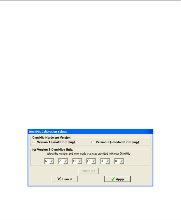
Each version 1 OmniMic is provided with a 6 character code (2 digits followed by 2 letters, then 2 more digits). The code characterizes the frequency response shape of the microphone as compared to a precision laboratory reference microphone, and is used by the OmniMic software program to correct during measurement.
To enter the code for your particular OmniMic into the program, select "Config > Mic ID" from the menu at the top of the screen, select "Version 1" microphone and select the 6 characters using the dropdown controls. Then click on "Apply".
Calibration Files:
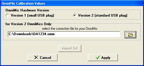
For Version 2 OmniMics and recalibrated Version 1 OmniMics, you can download the ".omm" calibration file as described above and then select "Config > Mic ID" from the menu at the top of the screen and then select "Version 2" microphone. Click the button showing the yellow folder and
5 | P a g e
browse to where you stored your ".omm" file. Then click "Apply".
Or if you are connected online with the computer you are using with OmniMic, click the "Web" button, enter the Version 2 code, and Omnimic will do the rest.
.
Sensitivity Readjustment
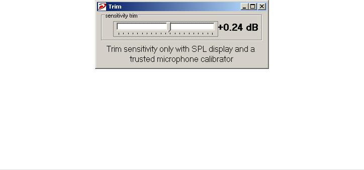
Over time, the sensitivity of microphones can drift to some degree. Provided reasonable care is taken to avoid exposure to high temperatures or humidity, their frequency response shapes typically remain stable, but if maximum level accuracy is required, you can trim the system senstivity relative to the value already included within the Calibration Code.
The sensitivity of the microphone can be checked with a trusted microphone calibrator and the OmniMic SPL/Spectrum display. If it is found to be in error, the senstivity can be adjusted by up to several decibels with the control that appears when you select "Config>Adjust" from the menu at the top of the screen.
6 | P a g e

Frequency Response
Index
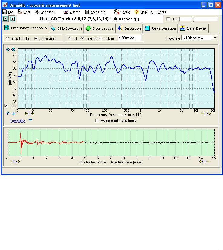
Use the Frequency Response analyzer to measure the frequency response or the impulse response.of a sound system.
Important! To use this properly you must be playing the specified audio track (from the OmniMic test track CD or DVD) as indicated at the top of the program window. The measurement
is matched to the test signals provided on the specified tracks. You can choose to use between two types of signal by selecting between the "pseudo noise" and "sine sweep" buttons above the graphs.
"Pseudo-noise" test signals, that sound like Pink Noise are easy on the ears for extended sessions. The accuracy using pseudo-noise at highest frequencies, however, can be degraded by sample clock variations
.
Sine Sweep signals provide the cleanest and most accurate measurements, as well as being able to drive speakers at specific SPL levels. This is the preferred choice for frequency response measurements and should be used for all high-frequency measurements
Frequency Response measurements will not operate correctly if you try to use normal Pink Noise test signals or any signal other than the one specified on the program window! The timing and spectral content of the files are critical for proper operation of OmniMic's synchronous frequency response measurement system.
Doing a Frequency Response measurement with OmniMic is easy -- essentially, you just play one of the proper Tracks, as indicated near the top of the form, set the microphone to pick up your system and the graph is shown on the screen. The OmniMic software also allows many adjustements which you can use to customize the graph or measurement. For
more Advanced functions, see the help section on that topic.
About Frequency Responses
Frequency Response is a curve that shows how strongly an audio system reproduces different parts of the frequency range. The curve will be higher on the graph at frequencies where the system plays louder, and lower (perhaps showing only varying background noise) at frequencies where the system plays weaker or not at all.
A perfect Frequency Response curve would look like a flat line over all frequencies. A typical one, though, will have variations of from 3 to 30 decibels ("dB") over most of the frequency range, and often dropping off at very low bass frequencies.
You can measure near individual speakers (about 1 meter away is best), or out in the room at various listening positions. The frequency response of a loudspeaker will be different at different places in the room. You can also use OmniMic to make an ongoing "average curve" over multiple positions (advanced) to give a typical frequency response curve.
A frequency response is related to its "impulse response" (the pressure signal that a speaker or sound system would make if it were fed by an extremely short pulse). OmniMic can
7 | P a g e

show impulse responses, and you can select how much of an impulse reponse you want to analyzer to look at when forming a frequency response. Click on the impulse response graph at the latest part of the impulse response you want OmniMic to include when it computes frequency response. The selected portion will appear as a red trace, the rest will remain black.
Reflections of sound in a room will appear as abrupt features in later parts of the impulse response (usually after about 3 to10 milliseconds from the main impulse response.). The response of the speaker without room reflections is smoother and less varied than when room reflections are included. Removal of room reflections is possible only at higher frequencies -- at lower frequencies, the reflections happen before even one full cycle of longer low frequency waves.
Because all audio frequencies are played at once in the pseudo noise signal, you cannot determine that the speaker is playing at any specific sound level at any individual frequency, so measurements with the psuedo noise show only relative response flatness. The curves are shown as values given in units of "dB". Also, minute variations in clock frequencies of different players can cause the response at higher frequencies can appear to vary when using pseudo noise. When high frequency accuracy is important, use the sine sweep signal.
To evaluate loudspeaker how frequency response changes at specific levels and for best accuracy at high frequencies, use the sine sweep to display curve values as "dBSPL" (sound pressure level).
In most cases, it is best to measure the frequency response of each speaker individually (i.e., have only one speaker at a time playing the Test Track signals). This will avoid interference effects from the two speakers complicating the graphs. However, in "all" (full room) responses, you may want to also measure with all speakers playing together.
Frequency Response Options:
"all": this setting shows a frequency response that includes all room echoes and reflections. In other words, the entire impulse response. In this view, impulse response itself is not shown.
"only to": for suppressing reflections. This is calculated only from the impulse response within the time selected. To select a different ending time, click the mouse at the desired time point within the impulse response graph. Impulse response information after the selected time will be excluded from the frequency response calculation. Select this time to exclude later reflections visible on the impulse response plot. Lower frequencies can't be measured using this option, limited by the length of the time selected. This mode works best when the OmniMic is relatively close to the loudspeakers.
"blended": blends from the "only to" calculation at higher frequencies, to the "all" calculation at lower frequencies. In other words, this mode removes echoes when it can, and doesn't when it can't.
smoothing: You can choose to smooth the frequency response graphs over 1 octave to 1/96th octave regions, to vary the amount of detail shown. An unsmoothed frequency response will be very ragged except when echoes are windowed or the measurement is taken very close to the loudspeakers.
Frequency Response measurement curves can be saved as "Added Curves" in FRD format using the "File, Save" menu. You can save either or both of the current "live" curve (currently produced by the microphone) or any displayed average curve. These can then be reloaded using the "Added Curves" menu so that multiple Added Curves can be shown on the same graph along with the "live" curve and the average curve. When Frequency Response files that contain these files are printed or saved in a "Snapshot", a list of legends
8 | P a g e
can be included. In snapshot files, a text note can also be added. FRD files or properly formatted ".txt" files can be loaded back into the Frequency Response plot.
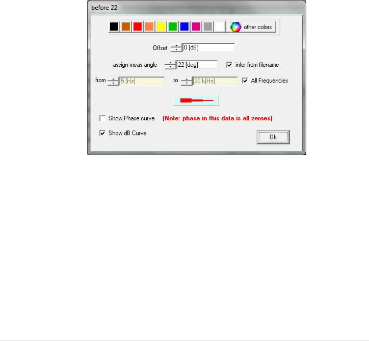
Up to 20 saved "Added" Frequency Response curves can be displayed on-screen, and can be individually offset in decibels from their saved levels. Their line thickness can be set narrrow or thin, and they can have another response from a saved file applied to further shape them ("Filter") or to unshape them ("Normalize"). Normalizing a curve by its own file will give a flat line.
Added Curves can also be associated with a "measurement angle" (and will try to infer this angle from the file name). This is to allow easy configuration of polar response plots.
You can also select the color of the curve, whether to show phase or dB (or both), and the frequency range over which to display each Added Curve.
The full set of curve filenames, along with their individual offset values (and any assigned measurement angles values) can be saved into a Curve List for easy retreival to the OmniMic screen. The first two curves specified can be used frequency response limit testing
(see Frequency Response: Advanced Mode).
You can alter the thickness of the displayed "live" Frequency Response curve by toggling (left-clicking) the small button that is just to the right of the "OmniMic" logo at bottom left of the graph. Right-clicking the button will change the thickness of the saved
or average curves.
The "Main Math" menu allows the llive Frequency Response curve to also have a Filter or a Normalizing response applied from a saved file. It can be evaluated for Pass/Fail testing (which checks whether the curve lies between the first two curves in the "added" curve list). Or it can be offset vertically or have its shape inverted. Curves saved with these applied will have the effects included in the saved file.
There are also a number of additional features for advanced users including phase responses, color polar displays, and watefall decay plots.
9 | P a g e
10 | P a g e
Frequency Response - Advanced Functions
Index
Additional Advanced features are built-in and available in the OmniMic Frequency Response analyzer for users who need to go into more depth in their measurements.
The advanced features are:
a set of Math functions so that you can measure responses
--as compared ("Normalized") to a saved file curve; This removes the effects of the curve used. If you normalized a curve by itself, you'd get a flat line.
--use file curves as a filter during measurement ("Filter"). If you Filtered a flat line with a curve, you'd get the Filter curve.
--sum (vector style, including phase) with a previously measured response from a FRD file
--offset, that is, moved up or down by a specified amound (in dB)
--with the response flipped (so that peaks are replaced with troughs and vice-versa)
--or have the OmniMic evaluate whether the displayed portion of a measurement falls entirely within the area between the first two specified file curves ("Evaluate within"). Offsets applied to the curve files during display are utilized for the evaluation (so you can use the same file for both limits, one offset upwards and the other offset downwards). You can also select whether to allow the program some vertical shifting to get the measured curve to fit (good for when you care about shape more than absolute sensitivity match).
Some of these functions utilize ".FRD" type text files as generated by OmniMic or other programs. These files can also be easily created using any text editor such as Windows' "Notepad", or a spreadsheet program.
measured responses can be arranged to be inverted in shape or offset vertically in dB.
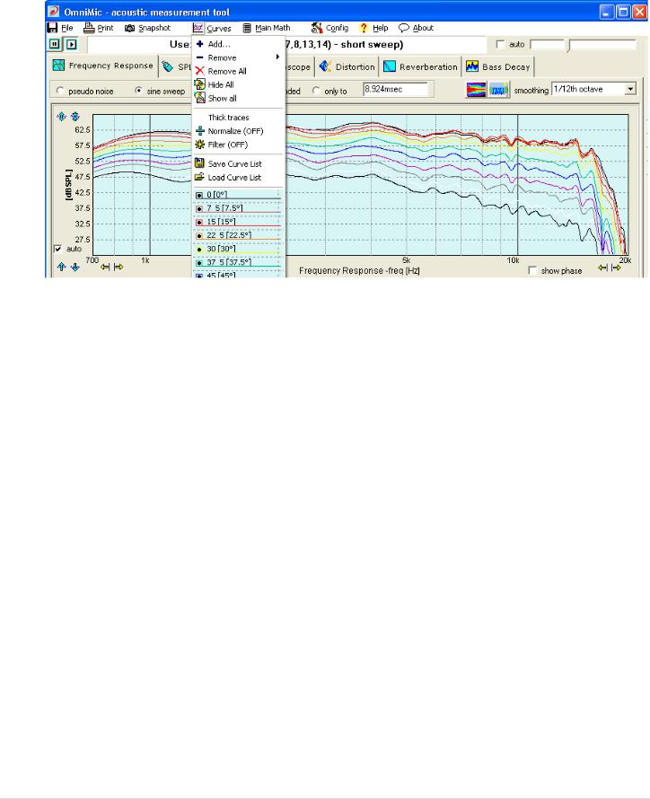
averaging: Left-click the "New Average" button to freeze the current frequency response curve on the graph (alternately, your keyboard's space bar can be used for this function). New live measured curves will be shown along with the frozen one. If you left-click it repeatedly, each current live curve will be averaged into the frozen curve (the button label will change to "more average" and indicate the number of averages included so far). This function is very useful for determining the average response curve over a range of listening positions in a room. Click "Clear Averages" to erase a frozen or averaged curve and show only the live curve. If you want to see only the frozen/ average curve, click on "Hide Main". You can save an average curve for later recall using the "File" menu, or recall a previous saved FRD file to replace the Average curve.
To average in a response curve that has been previously saved to a file via the file menu, first "Add" the curve to the display using the "Curves" menu. Then Right-click on the "New Average" or "more Averages" button to include the last Added file to the average curve.
An option to show the impulse response plot in "logarithmic" form rather than the usual "linear" form. Logarithmic form hides polarity but makes it easier to look at the decay shape of an impulse response curve. With logarithmic display it is often easier to identify discrete reflections in the impulse response, which can be particularly helpful with Waterfall Displays.
Two styles of color 3D Polar displays, for diplaying responses in sets of saved files in formats that show how the frequency response of a speaker varies as it radiates into different
11 | P a g e

directions. To use these, there must be at least three added curves in the main frequency response plot, each with different radiation angles assigned. See: Polar displays.
Three different styles of Waterfall graphs can be made from impulse responses. When the Waterfall button (just to the left of the smoothing control) is pressed, the OmniMic form shows the impulse response being measured at the bottom of the screen and a Waterfall plot above it. For more about making Waterfalls, see: Waterfalls.
You can also display the phase response of the loudspeaker by selecting the checkbox shown at bottom right below the frequency response graph. Phase display works with the "only to" or "blended" options. You can use the delay adjustment (lower right part of the screen) to specify an amount of delay you wish applied to the phase display. At zero delay, the time reference is the instant that the peak of the impulse response arrives at the microphone. (Note that averaging does not operate on phase responses).
Absolute time references: OmniMic always aligns "0 ms" to occur at the highest peak in the impulse response. Normally, the frequency response calculates from this point forward, and the peak of the response will be the time reference plane. In advanced mode, you can also select to have OmniMic start calculation from a different first point. If you wish to see only the response resulting from a later peak (and if the first "highest" impulse response has decayed sufficiently by then to not interfere), right-click the mouse on the impulse response at the starting point of the portion you wish to include.
With some computers, you can play the frequency response test signals (the pseudo noise or the short swept sine) out from a soundcard in the computer rather than playing the needed signals from a CD. To enable this, position the mouse over the "status bar" (the horizontal area at the bottom of the OmniMic window), hold down the "Shift" and the "Alt" keys, and click the mouse button.
See also "Playing OmniMic test tracks without a CD" for other ways to play the test signals.
12 | P a g e

Frequency Response: Waterfalls
Index
Waterfall plots are used by driver and loudspeaker designers for driver selection, to identify resonances or reflections, and to view driver and waveguide behavior.
The Waterfall feature becomes available when you click the Waterfall button (above the Frequency Response graph, next to the Smoothing control). Waterfalls are calculated from the impulse response.
What does a Waterfall mean?
A waterfall is an attempt to illustrate on a 3-D graph how the energy decays or is radiated over a range of frequencies. OmniMic includes three different styles of waterfall processes, selectable via the "Waterfall Type" menu.
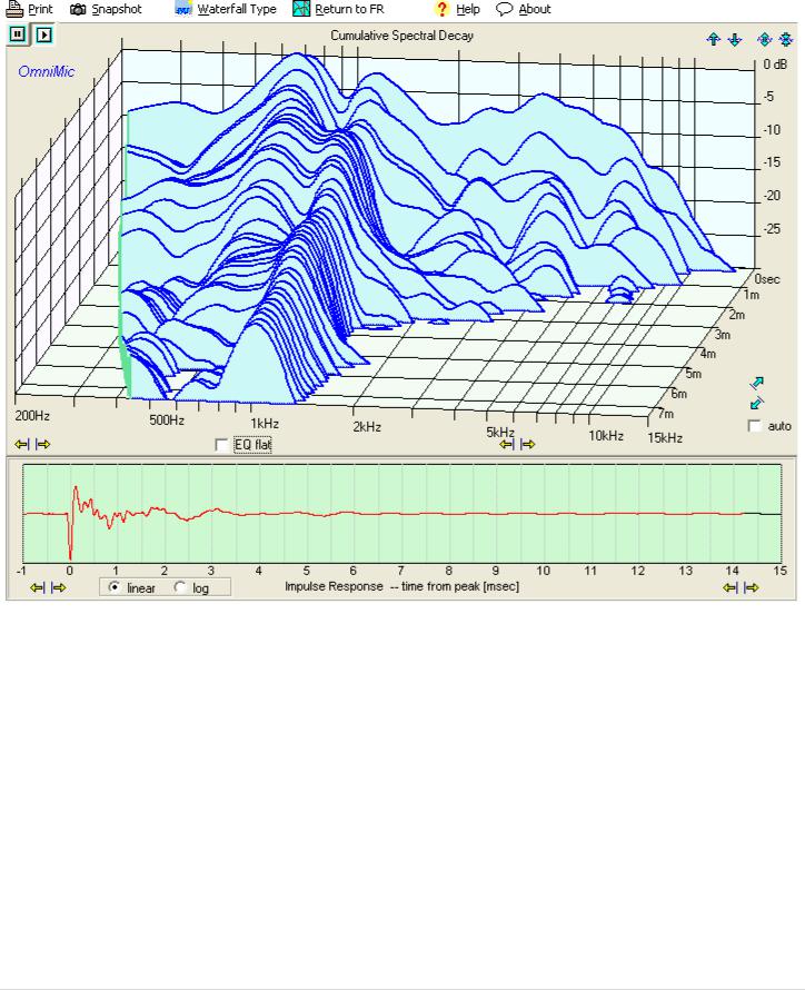
A "Cumulative Spectral Decay", or "CSD" waterfall shows a series of time slices approximately indicating the contribution to the total response that is made after the time instant shown in the axis going into the screen. When a loudspeaker is driven with an electrical impulse, the pressure it creates should ideally also represent a pressure impulse. But loudspeaker drivers aren't ideal so they also generate resonances -- pressure waves that decay more slowly at various frequencies. The effects of echoes can hide the resonances in a CSD waterfall, but at higher frequencies the echoes can be removed by "Windowing" the calculation to only include the part of the Impulse Response that occurs before the first reflection (from a surface such as a wall or furniture) reaches the OmniMic. Careful choice of positioning within the Impulse Response is critical, because the effects of any reflections included within the selected portion will contaminate all regions of the graph up to that point on the time axis. Below some frequency determined by where the Impulse Response is clicked and how far along on the time (depth) axis a trace exists, meaningful calculation cannot be done. The graph curve is chopped off at those points on the waterfall display.
The CSD waterfall calculation process introduces some spurious side effects, so the graph should be viewed in general terms. Exact values along the curves of waterfalls are not usually reliable, rather, the positions and sizes of decaying forward-approaching ridges on the graph indicate frequency and relative intensities of resonances.
CSD waterfall curves can now be shown with different degrees of smoothing, and can also be use with long time lengths (to 250 milliseconds) for viewing effects of room reflections.
13 | P a g e
"Toneburst Energy Storage" shows the effect that would occur if the loudspeaker were driven by short tonebursts of energy one at at time, concentrated near each test frequency. The speaker output would ideally end after the toneburst ended, but realworld devices will continue to ring as the energy stored within dies out. This is similar to a test devised by Linkwitz. The Toneburst Energy Storage data in OmniMic is calculated from a measured impulse response, and the number of applied toneburst cycles can be selected using a control at the bottom right. Like the CSD waterfall, the impulse response can be windowed to remove effects of reflections.
The grey area shows the energy that is expected if there were no storage or hangover. The light-blue area forward of that is the stored (delayed) energy at the indicated frequency.
The CSD and Toneburst Energy Storage waterfall plots are useful identifying moderate to high Q resonances in a drivers's frequency response. The audibility of the features easily identified in these waterfall plots is somewhat controversial, with some research (see Toole) indicating that the higher Q resonances seen in waterfall displays are significantly less audible than low-Q resonances that do not stand out in CSD or TES waterfall displays. In any event, it should be remembered that waterfall data (and also frequency response data) are simply alternate presentations of information contained within impulse responses.
14 | P a g e

"Wavelet Spectrogram" shows a combined time/frequency representation of the impulse response. The Wavelet Spectrogram in OmniMic uses a very fast algorithm that allows the display to occur in real time. In all time/frequency displays there is a mathematical "uncertainty principle" which limits the degree of time resolution that can be obtained for a given frequency resolution, and vice versa. In other words, the more detailed the time character of the display, the less detailed will be the frequency character. The Wavelet Spectrogram shows the optimized presentation, giving as much combined resolution as possible. The horizontal axis is time, the vertical axis is frequency, and color shows the relative intensity (in dB). You can select the octave resolution, in a control below the plot, to determine the desired resolution tradeoff. An ideal wavelet spectrogram (flat response, no resonances or reflections) will look like a vertical tapered horn, like this:
15 | P a g e
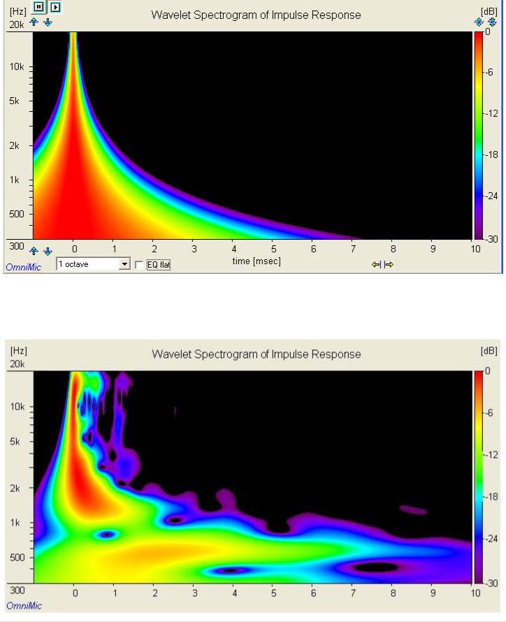
The time resolution is more detailed at higher frequencies than at lower frequencies (because there are more "Hz" in an octave at high frequencies than at lower frequencies).
A typical loudspeaker will show a less clear graph, with smearing at various frequencies and additional color features appearing at later times where reflection or diffraction occur.
16 | P a g e

If you spread the time axis out to full length, you can also use the Wavelet Spectrogram for viewing room reflections and the frequency ranges over which they predominate.
Features of the Waterfall Displays
For CSD and TES type waterfalls, the top of the screen reference line is set by the largest feature over the selected frequency range. Both types also allow selection of an "EQ flat" function that adjusts gain at each frequency, as if an ideal equalizer were applied. Time is shown on the "depth" axis. You can click at the end of a line trace on the labeled axes (time for CSD, frequency for Toneburst) to highlight the single line in a waterfall plot for easier reading.
For CSD and TES, the position where you click within the Impulse Response graph below determines the length of the waterfall calculation, starting from 0ms..
For the Wavelet Spectrograms, the red color indicates the highest decibel level in the frequency range. The "EQ flat" button can be used so that red instead indicates the highest level at each frequency (in effect, what would be obtained if the speaker could be equalized flat without affecting its phase). Impulse response windowing
will not have an effect on Wavelet Spectrogram displays.
The three dimensions (intensity, frequency, and time) of the graph can be adjusted as desired for display using scaling controls similar to those on the other OmniMIc graphs.
As with the rest of the OmniMic graphs, there are buttons provided for both taking Snapshots of graphs or for sending copies of the screen display to a printer (if installed on your computer).
Often selection of the Log format display of the Impulse Response graph below will allow for easier location of strong reflections.
To return to the normal Frequency Response page of OmniMic, click on the "Return to FR" menu button.
17 | P a g e
Determining Z-Offset (depth offset) between speaker drivers
Index
A major advantage of Omnimic over other audio measurement systems is that it doesn't require a signal connection between the computer and the audio system or speaker being measured. You can measure system response without needing access to electrical connections simply by playing a test CD or audio file. That's very handy.
But there is a complication that comes with this convenience, which is that without a hard connection Omnimic has no way of knowing the precise time at which a signal it is sensing left the loudspeaker. Omnimic determines timing by finding the largest peak in the measured impulse response and referencing that in its phase determinations. When generating files for loudspeaker design, it is important to know the relative delay between drivers in the loudspeaker system. If a midrange driver is recessed in a baffle this will typically require a different crossover circuit than if the midrange is flush mounted on a baffle. Different drivers have different amounts of depth, or "z position" of the originating point of the sound waves they generate. What is important to know is not the absolute location of the acoustic origin of each driver, but the relative "z offset" between two drivers for which a crossover section is being designed.
Omnimic now has a new feature to provide accurate determination of the z-offset between pairs of drivers. This feature is based on a method described by Jeff Bagby for use with his PCD software, in which separate measurements are made of each driver, and then those files are then combined mathematically and compared to a measurement that was made with both drivers playing simultaneously. Bringing this process into OmniMic limits the number of files that have to be exported from OmniMic to PCD and simplifies the steps for the user.
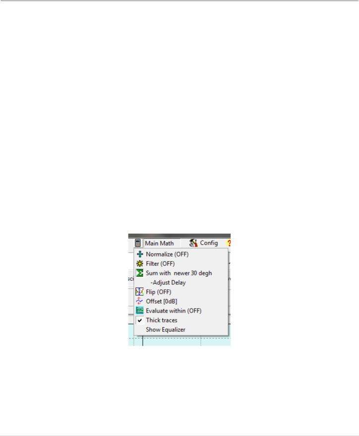
The feature uses a new math process for live ("Main") curve in Omnimic, which is a vector "Sum" function. This can be found in the "Main Math" menu of the Frequency Response screen. When this is chosen (and an appropriate FRD file is selected for summing with any new measured responses), the Main curve will be that of what is actually measured, summed with the specified FRD file. For this to be reasonable, the saved FRD file must have valid phase information, so make sure that the "show phase" checkbox is checked when saving FRD files to be summed with!
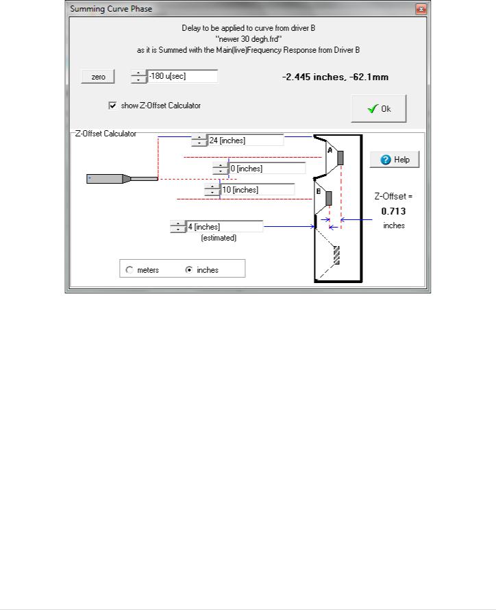
After a file has been chosen, a new menu option appears (see above), "Adjust Delay". Clicking this brings up a new form with a control that lets you select the delay to be applied to the chosen file before it is summed with new measured responses. If you check the box labeled "show Z-Offset Calculator", the form will expand to show a diagram and controls which can calculate the proper Z-offset values to use in PCD.
18 | P a g e
________________________________________
How to use the Z-Offset Calculator:
1). Position your microphone at the design center point (often on-axis with driver "A", usually the higher frequency driver, such as the tweeter if measuring a tweeter/midrange pair).
2). Make sure that "show phase" is checked on the Frequency Response screen. Measure the response of driver "B" playing at moderately low level alone with the microphone at this position. Save this file to disk.
3). Connect so that both drivers "A" and "B" play simultaneously (use a blocking capacitor to protect tweeters, of course, and be careful of levels -- these measurements need not be done at high level!) and save that to file also.
4). Use the "Added Curves">"Add" menu to add the newly saved file (of both drivers together) to the display.
5) Now go to the "Main Math">"Sum" menu and select the first curve (of driver "B" playing alone). Then click "Main Math">"Adjust Delay" to bering up the form shown above. Put a check in its "Show Z-Axis Calculator" checkbox.
6) Get out a tape measure and measure the distances shown in the figure (in either meters or inches), enter them in the boxes. Enter an estimate for the distance from the baffle to the voice coil of driver B (this need not be highly accurate, within several inches should be fine).
7) Uncheck the "show phase" box on the Frequency Response screen. Now, while measuring driver "A" alone (the display of which is now summed with driver "B''s curve), adjust the control (in seconds) at the top of the new form until the measured response curve best matches the magnitude (not necessarily phase!) of the Added Curve that shows the actual measurement of both drivers together. When this is correct, then the value of Z axis offset will be shown at the bottom right of the form. THIS (IN METERS) IS THE Z VALUE YOU WOULD ENTER FOR DRIVER B in PCD, if driver A uses a Z axis position of 0.
8) Turn off the "Sum" function for Main Math, and measure (and save) the data from driver A playing alone for use in PCD with driver B's curve taken initially.
19 | P a g e
 Loading...