

Page 1
3B SCIENTIFIC3B SCIENTIFIC
3B SCIENTIFIC®
3B SCIENTIFIC3B SCIENTIFIC
PHYSICSPHYSICS
PHYSICS
PHYSICSPHYSICS
U15040 Torsion pendulum according to Professor Pohl
Operating instructions
12/03 ALF
9
8
7
6
5
4
bl bm bn bo bp
bq br bs
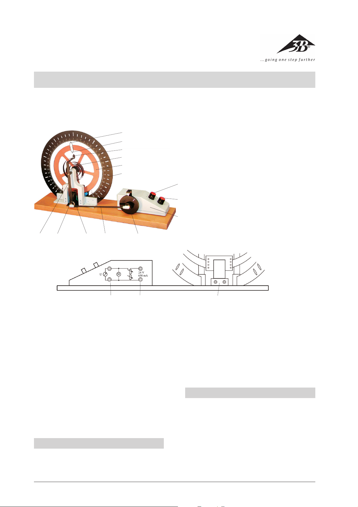
1 Exciter motor
2 Control knob for fine adjustment of the exciter voltage
3 Control knob for coarse adjustment of the exciter voltage
4 Scale ring
5 Pendulum body
6 Coil spring
7 Pointer for the exciter phase angle
8 Pointer for the pendulum’s phase angle
9 Pointer for the pendulum’s deflection
3
bl Exciter
bm Eddy current brake
bn Guide slot and screw to set the exciter amplitude
2
bo Connecting rod
bp Eccentric drive wheel
bq 4-mm safety socket for exciter voltage measurement
1
br 4-mm safety sockets for the exciter motor power supply
bs 4-mm safety sockets for the eddy current brake power
supply
The torsion pendulum may be used to investigate free,
forced and chaotic oscillations with various degrees of
damping.
Experiment topics:
• Free rotary oscillations at various degrees of damp-
ing (oscillations with light damping, aperiodic oscillation and aperiodic limit)
• Forced rotary oscillations and their resonance
curves at various degrees of damping
• Phase displacement between the exciter and reso-
nator during resonance
• Chaotic rotary oscillations
• Static determination of the direction variable D
• Dynamic determination of the moment of inertia J
1. Safety instructions
• When removing the torsional pendulum from the
packaging do not touch the scale ring. This could
lead to damage. Always remove using the handles
provided in the internal packaging.
• When carrying the torsional pendulum always hold
it by the base plate.
• Never exceed the maximum permissible supply
voltage for the exciter motor (24 V DC).
• Do not subject the torsional pendulum to any un-
necessary mechanical stress.
2. Description, technical data
The Professor Pohl torsional pendulum consists of a
wooden base plate with an oscillating system and an
electric motor mounted on top. The oscillating system
is a ball-bearing mounted copper wheel (5), which is
connected to the exciter rod via a coil spring (6) that
provides the restoring torque. A DC motor with coarse
and fine speed adjustment is used to excite the torsional pendulum. Excitement is brought about via an
eccentric wheel (14) with connecting rod (13) which
6
Page 2

unwinds the coil spring then compresses it again in a
periodic sequence and thereby initiates the oscillation
of the copper wheel. The electromagnetic eddy current brake (11) is used for damping. A scale ring (4)
with slots and a scale in 2-mm divisions extends over
the outside of the oscillating system; indicators are
located on the exciter and resonator.
The device can also be used in shadow projection demonstrations.
A DC power supply unit for the torsional pendulum
U11755 is required to power the equipment.
Natural frequency: 0.5 Hz approx.
Exciter frequency: 0 to 1.3 Hz (continuously adjustable)
Terminals:
Motor: max. 24 V DC, 0.7 A,
via 4-mm safety sockets
Eddy current brake: 0 to 24 V DC, max. 2 A,
via 4-mm safety sockets
Scale ring: 300 mm Ø
Dimensions: 400 mm x 140 mm x 270 mm
Ground: 4 kg
2.1 Scope of supply
1 Torsional pendulum
2 Additional 10 g weights
2 Additional 20 g weights
3. Theoretical Fundamentals
3.1 Symbols used in the equations
D = Angular directional variable
J = Mass moment of inertia
M = Restoring torque
T = Period
T0= Period of an undamped system
Td= Period of the damped system
= Amplitude of the exciter moment
M
E
b = Damping torque
n = Frequency
t = Time
Λ = Logarithmic decrement
δ = Damping constant
ϕ
= Angle of deflection
ϕ
= Amplitude at time t = 0 s
0
ϕ
= Amplitude after n periods
n
ϕ
= Exciter amplitude
E
ϕ
= System amplitude
S
ω0= Natural frequency of the oscillating system
ωd= Natural frequency of the damped system
ωE= Exciter angular frequency
ωE
= Exciter angular frequency for max. amplitude
res
Ψ0S= System zero phase angle
3.2 Harmonic rotary oscillation
A harmonic oscillation is produced when the restoring
torque is proportional to the deflection. In the case of
harmonic rotary oscillations the restoring torque is
proportional to the deflection angle ϕ:
M = D ·
ϕ
The coefficient of proportionality D (angular direction
variable) can be computed by measuring the deflection angle and the deflection moment.
If the period duration T is measured, the natural resonant frequency of the system ω0 is given by
ω
= 2 π/T
0
and the mass moment of inertia J is given by
D
2
ω
=
0
J
3.3 Free damped rotary oscillations
An oscillating system that suffers energy loss due to
friction, without the loss of energy being compensated
for by any additional external source, experiences a
constant drop in amplitude, i.e. the oscillation is
damped.
At the same time the damping torque b is proportional
to the deflectional angle
.
ϕ
.
The following motion equation is obtained for the
torque at equilibrium
.
..
JbD⋅+⋅+⋅=
ϕϕϕ
0
b = 0 for undamped oscillation.
If the oscillation begins with maximum amplitude
ϕ
at t = 0 s the resulting solution to the differential equation for light damping (δ² < ω0²) (oscillation) is as follows
–δ ·t
ϕ
ϕ
=
· e
· cos (
ω
0
d
· t)
δ = b/2 J is the damping constant and
2
ωωδ
=−
d
2
0
the natural frequency of the damped system.
Under heavy damping (δ² > ω0²) the system does not
oscillate but moves directly into a state of rest or equilibrium (non-oscillating case).
The period duration Td of the lightly damped oscillating system varies only slightly from T0 of the undamped
oscillating system if the damping is not excessive.
By inserting t = n · Td into the equation
–δ ·t
ϕ
ϕ =
and ϕ =
ϕ
tain the following with the relationship
ϕ
ϕ
· e
· cos (
ω
0
for the amplitude after n periods we ob-
n
n
0
δ
−⋅
n
=⋅
eT
d
d
· t)
ω
= 2 π/T
d
d
and thus from this the logarithmic decrement Λ:
Λ
=⋅ =⋅
δ
T
d
ϕ
1
In In
n
ϕ
n
0
ϕ
n
=
ϕ
n+1
0
7
Page 3

By inserting δ = Λ / Td ,
Ψ
ω
= 2 π / T0 and
0
ω
= 2π / T
d
into the equation
2
ωωδ
=−
d
2
0
we obtain:
2
TT
=⋅+1
d0
Λ
2
4
π
whereby the period Td can be calculated precisely provided that T0 is known.
3.4 Forced oscillations
In the case of forced oscillations a rotating motion with
sinusoidally varying torque is externally applied to the
system. This exciter torque can be incorporated into
the motion equation as follows:
.
..
JbD M t⋅+⋅+⋅= ⋅ ⋅
ϕϕϕ ω
sin
E
()
E
After a transient or settling period the torsion pendulum oscillates in a steady state with the same angular
frequency as the exciter, at the same time ωE can still
be phase displaced with respect to ω0. Ψ0S is the system’s zero-phase angle, the phase displacement between the oscillating system and the exciter.
ϕ
ϕ
=
· sin (
ω
· t –
Ψ
S
E
The following holds true for the system amplitude
M
ϕ
=
ωω δω
()
02E
J
2
2
−
)
0S
E
2
+⋅
4
ϕ
2
E
The following holds true for the ratio of system amplitude to the exciter amplitude
M
ϕ
S
=
ϕ
E
ω
E
−
14
ω
0
E
J
2
2
+
2
δ
ω
0
2
ω
E
⋅
ω
0
d
Stronger damping does not result in excessive amplitude.
For the system’s zero phase angle Ψ0S the following is
true:
arctan
ωω
=
0S
δω
2
22
−
ω
0
For ωE = ω0 (resonance case) the system’s zero-phase
angle is Ψ0S = 90°. This is also true for δ = 0 and the
oscillation passes its limit at this value.
In the case of damped oscillations (δ > 0) where
ωE < ω0, we find that 0° ≤ Ψ0S ≤ 90° and when ωE > ω
0
it is found that 90° ≤ Ψ0S ≤ 180°.
In the case of undamped oscillations (δ = 0), Ψ0S = 0°
for ωE < ω0 and Ψ0S = 180° for ωE > ω0.
4. Operation
4.1 Free damped rotary oscillations
• Connect the eddy current brake to the variable volt-
age output of the DC power supply for torsion pendulum.
• Connect the ammeter into the circuit.
• Determine the damping constant as a function of
the current.
4.2 Forced oscillations
S
• Connect the fixed voltage output of the DC power
supply for the torsion pendulum to the sockets (16)
of the exciter motor.
• Connect the voltmeter to the sockets (15) of the
exciter motor.
• Determine the oscillation amplitude as a function
of the exciter frequency and of the supply voltage.
• If needed connect the eddy current brake to the
variable voltage output of the DC power supply for
the torsion pendulum.
4.3 Chaotic oscillations
• To generate chaotic oscillations there are 4 supple-
mentary weights at your disposal which alter the
torsion pendulum’s linear restoring torque.
• To do this screw the supplementary weight to the
body of the pendulum (5).
In the case of undamped oscillations, theoretically
speaking the amplitude for resonance (ωE equal to ω0)
increases infinitely and can lead to “catastrophic resonance”.
In the case of damped oscillations with light damping
the system amplitude reaches a maximum where the
exciter’s angular frequency ω
is lower than the sys-
E res
tem’s natural frequency. This frequency is given by
2
δ
ωω
=⋅−1
Eres 0
2
2
ω
0
8
Page 4

5. Example experiments
5.1 Free damped rotary oscillations
• To determine the logarithmic decrement Λ, the
amplitudes are measured and averaged out over
several runs. To do this the left and right deflections of the torsional pendulum are read off the
scale in two sequences of measurements.
• The starting point of the pendulum body is located
at +15 or –15 on the scale. Take the readings for
five deflections.
• From the ratio of the amplitudes we obtain Λ us-
ing the following equation
ϕ
n
Λ
=
In
n
ϕ
n+1
ϕ
–
ϕ
+
0 –15 –15 –15 –15 15 15 15 15
1 –14.8 –14.8 –14.8 –14.8 14.8 14.8 14.8 14.8
2 –14.4 –14.6 –14.4 –14.6 14.4 14.4 14.6 14.4
3 –14.2 –14.4 –14.0 –14.2 14.0 14.2 14.2 14.0
4 –13.8 –14.0 –13.6 –14.0 13.8 13.8 14.0 13.8
5 –13.6 –13.8 –13.4 –13.6 13.4 13.4 13.6 13.6
nØ
ϕ
– Ø
ϕ
+
Λ
–
Λ
+
0 –15 15
1 –14.8 14.8 0.013 0.013
2 –14.5 14.5 0.02 0.02
3 –14.2 14.1 0.021 0.028
4 –13.8 13.8 0.028 0.022
5 –13.6 13.5 0.015 0.022
• The average value for Λ comes to Λ = 0.0202.
• For the pendulum oscillation period T the follow-
ing is true: t = n · T. To measure this, record the
time for 10 oscillations using a stop watch and calculate T.
T = 1.9 s
• From these values the damping constant δ can be
determined from δ = Λ / T.
δ
= 0.0106 s
–1
• For the natural frequency ω the following holds
true
2
π
2
ω
=
ω
= 3.307 Hz
T
2
δ
−
5.2 Free damped rotary oscillations
• To determine the damping constant δ as a function of the current Ι flowing through the electromagnets the same experiment is conducted with
an eddy current brake connected at currents of
Ι = 0.2 A, 0.4 A and 0.6 A.
ΙΙ
Ι = 0.2 A
ΙΙ
n
ϕ
– Ø
ϕ
– Λ –
0 –15 –15 –15 –15 –15
1 –13.6 –13.8 –13.8 –13.6 –13.7 0.0906
2 –12.6 –12.8 –12.6 –12.4 –12.6 0.13
3 –11.4 –11.8 –11.6 –11.4 –11.5 0.0913
4 –10.4 –10.6 –10.4 –10.4 –10.5 0.0909
5 9.2 –9.6 –9.6 –9.6 –9.5 0.1
• For T = 1.9 s and the average value of Λ = 0.1006
we obtain the damping constant: δ = 0.053 s
ΙΙ
Ι = 0.4 A
ΙΙ
n
ϕ
– Ø
ϕ
– Λ –
–1
0 –15 –15 –15 –15 –15
1 –11.8 –11.8 –11.6 –11.6 –11.7 0.248
2 –9.2 –9.0 –9.0 –9.2 –9.1 0.25
3 –7.2 –7.2 –7.0 –7.0 –7.1 0.248
4 –5.8 –5.6 –5.4 –5.2 –5.5 0.25
5 –4.2 –4.2 –4.0 –4.0 –4.1 0.29
• For T = 1.9 s and an average value of Λ = 0.257 we
ϕ
– Λ –
–1
obtain the damping constant: δ = 0.135 s
ΙΙ
Ι = 0.6 A
ΙΙ
n
ϕ
– Ø
0 –15 –15 –15 –15 –15
1 –9.2 –9.4 –9.2 –9.2 –9.3 0.478
2 –5.4 –5.2 –5.6 –5.8 –5.5 0.525
3 –3.2 –3.2 –3.2 –3.4 –3.3 0.51
4 –1.6 –1.8 –1.8 –1.8 –1.8 0.606
5 –0.8 –0.8 –0.8 –0.8 –0.8 0.81
• For T = 1.9 s and an average value of Λ = 0.5858
we obtain the damping constant: δ = 0.308 s
–1
5.3 Forced rotary oscillation
• Take a reading of the maximum deflection of the
pendulum body to determine the oscillation amplitude as a function of the exciter frequency or
the supply voltage.
T = 1.9 s
Motor voltage V
ϕ
3 0.8
4 1.1
5 1.2
6 1.6
7 3.3
7.6 20.0
8 16.8
9 1.6
10 1.1
9
Page 5

• After measuring the period T the natural frequency
of the system ω0 can be obtained from
ω
= 2 π/T = 3.3069 Hz
0
• The most extreme deflection arises at a motor voltage of 7.6 V, i.e. the resonance case occurs.
• Then the same experiment is performed with an
eddy current brake connected at currents of
Ι = 0.2 A, 0.4 A and 0.6 A.
ΙΙ
Ι = 0.2 A
ΙΙ
Motor voltage V
ϕ
3.0 0.9
4.0 1.1
5.0 1.2
6.0 1.7
7.0 2.9
7.6 15.2
8.0 4.3
9.0 1.8
10.0 1.1
ΙΙ
Ι = 0.6 A
ΙΙ
Motor voltage V
5.0 1.3
6.0 1.8
7.0 3.6
7.6 7.4
8.0 3.6
9.0 1.6
10.0 1.0
3.0 0.9
4.0 1.1
5.0 1.2
6.0 1.6
7.0 2.8
7.6.0 3.6
8.0 2.6
9.0 1.3
10.0 1.0
ϕ
ΙΙ
Ι = 0.4 A
ΙΙ
Motor voltage V
3.0 0.9
4.0 1.1
A
[skt]
20
15
10
• From these measurements the resonance curves can
be plotted in a graph depicting the amplitudes
ϕ
against the motor voltage.
• The resonant frequency can be determined by find-
ing the half-width value from the graph.
I=0,0A
I=0,2A
I=0,4A
5
1
012
Resonance curves
3
3B Scientific GmbH • Rudorffweg 8 • 21031 Hamburg • Germany • www.3bscientific.com • Technical amendments may occur
567 8910
4
10
I=0,6A
u[v]
 Loading...