

Page 1

YSI ADV6600
Environmental Monitoring System
Operations
Manual
Page 2

Page 3

Table of Contents
Table of Contents.....................................................................................................3
Section 1. Introduction to the ADV6600..........................................................1
1-1. About the ADV6600 ......................................................................................1
1-2. About YSI, Inc...............................................................................................1
1-3. How to Use This Manual...............................................................................2
1-4. Unpacking and Inspection............................................................................3
1-5. Safety Considerations....................................................................................3
Section 2. Preparing the System for Field Studies..........................................5
2-1. Preparing the Dissolved Oxygen Probe.......................................................5
2-1.1. Preparation of the DO Electrolyte Solution...................................................................... 5
2-1.2. Membrane Installation without the DO Probe Installed in the Sonde............................... 5
2-1.3. Membrane Installation with the DO Probe Installed in the Sonde.................................... 6
2-2. Installing Water Quality Probes..................................................................8
2-2.1. Removing the Port Plugs...................................................................................................8
2-2.2. Bulkhead Diagram............................................................................................................ 9
2-2.3. O-Ring Lubrication......................................................................................................... 10
2-2.4. Installing the Optical Probes........................................................................................... 10
2-2.5. Installing the Conductivity/Temperature, DO, and pH/ORP Probes .............................. 10
2-2.6. Installing the ISE Probes................................................................................................. 10
2-2.7. Installing the Probe Guard.............................................................................................. 11
2-3. Attaching Your Sonde to a Computer.......................................................11
2-3.1. Installing the Batteries .................................................................................................... 11
2-3.2. Preparing the Cable......................................................................................................... 12
2-3.3. Using the AC Power Supply........................................................................................... 12
2-3.4. Attaching the Cable......................................................................................................... 13
Section 3. Configuring Your ADV6600 – Installation of ADVantage 6600
Software and Sonde Firmware Set-up .................................................................15
3-1. ADVantage 6600 Software – System Requirements.................................15
3-2. Installing ADVantage 6600 Software ........................................................15
3-3. Launching the Software..............................................................................15
ADV6600 Y S I Environmental iii
Page 4

Table of Contents
3-4. Connecting to the System............................................................................16
Settings....................................................................................................................... ............... 16
Baud Rate.................................................................................................................................. 17
3-5. Understanding the Firmware of the ADV6600.........................................18
3-6. Setting up the Water Quality Sensor Firmware.......................................18
3-6.1. Setting Up the Water Quality Sensors ............................................................................ 18
3-6.2. Water Quality Menu Flowchart...................................................................................... 20
3-6.3. Setting Up Installed Sensors........................................................................................... 21
3-6.4. Setting Up Reports.......................................................................................................... 21
3-6.5. Advanced Menu Features................................................................................................24
3-7. Setting up the ADV Sensor Firmware.......................................................28
3-7.1. Setting the System Time................................................................................................. 28
3-7.2. Setting Up the ADV Parameter Output........................................................................... 28
3-8. Exiting the ADV6600 Firmware ................................................................30
3-9. ADV6600 Firmware Upgrades...................................................................30
Section 4. Calibration and Diagnostics..........................................................35
4-1. Beam Check Basics......................................................................................35
4-2. Running the ADV Beam Check .................................................................35
4-2.1. Laboratory Beam Check Procedure................................................................................ 36
4-2.2. Creating a Beam Check File........................................................................................... 38
4-2.3. Opening a Recorded Beam Check File........................................................................... 38
4-2.4. Viewing a Recorded Beam Check File........................................................................... 40
4-2.5. Interpreting Your Laboratory Beam Check Data............................................................ 40
4-2.6. Beam Check Feature Summary....................................................................................... 42
4-3. Calibrating the Compass ............................................................................43
Compass Calibration Procedure................................................................................................ 44
4-4. Changing the Pressure Sensor Offset........................................................45
4-5. Water Quality Sensors – Preparing for Calibration................................46
4-5.1. Health and Safety............................................................................................................ 47
4-5.2. Materials Required.......................................................................................................... 47
4-5.3. Calibration Tips .............................................................................................................. 47
4-5.4. Use of the Calibration Cup.............................................................................................. 48
4-5.5. Recommended Volumes of Calibration Reagents........................................................... 49
4-6. Water Quality Sensors - Calibration Procedures.....................................49
4-6.1. Temperature.................................................................................................................... 50
4-6.2. Conductivity.................................................................................................................... 50
4-6.3. Dissolved Oxygen for Unattended Monitoring Studies.................................................. 51
4-6.4. Dissolved Oxygen for Spot Sampling Studies................................................................ 52
4-6.5. pH ................................................................................................................................... 52
4-6.6. ORP................................................................................................................................. 53
ADV6600 Y S I Environmental Page iv
Page 5

Table of Contents
4-6.7. Ammonium..................................................................................................................... 54
4-6.8. Nitrate............................................................................................................................. 56
4-6.9. Chloride .......................................................................................................................... 57
4-6.10. Turbidity ....................................................................................................................... 59
4-6.11. Chlorophyll................................................................................................................... 61
4-6.12. Rhodamine WT............................................................................................................. 64
4-7. Establishing Default Calibration – “UNCAL” Command......................66
Section 5. Field Mounting and Installation...................................................67
5-1. Mounting Methods......................................................................................67
5-1.1. Deploying Using the YSI 6650 Clamps.......................................................................... 68
5-1.2. Deploying in a PVC Pipe................................................................................................ 70
5-1.3. Deploying on a Simple Tether........................................................................................ 72
5-2. Mounting Cautions......................................................................................73
5-2.1. Bottom Interference........................................................................................................ 73
5-2.2. Flow Interference............................................................................................................ 75
5-2.3. Interference from Magnetic Material.............................................................................. 75
Section 6. Using Your ADV6600 In The Field..............................................77
6-1. Checking Your Battery Voltage.................................................................77
6-2. Real-time Data Collection...........................................................................78
6-3. Unattended Data Collection........................................................................79
6-4. SDI-12 Data Collection................................................................................82
Section 7. Downloading ADV6600 Data........................................................87
7-1. Important Information on Downloading Data.........................................87
7-2. Data Location – Features of the Recorder ................................................87
7-3. Data Download Procedure..........................................................................89
Section 8. ADVantage 6600 Software – Post-Processing of Data................91
8-1. Opening a Saved File...................................................................................91
8-1.1. Workspaces..................................................................................................................... 91
8-2. Exporting Data to a Spreadsheet ...............................................................92
8-3. Using the Visual Data Display....................................................................93
8-4. Toolbars........................................................................................................95
8-4.1. Main Toolbar .................................................................................................................. 95
8-4.2. Data Toolbar................................................................................................................... 95
8-4.3. Display Toolbar .............................................................................................................. 95
8-4.4. Data Collection Toolbar..................................................................................................96
8-5. Menu Features.............................................................................................96
ADV6600 Y S I Environmental Page v
Page 6

Table of Contents
8-5.1. File.................................................................................................................................. 96
8-5.2. Edit.................................................................................................................................. 97
8-5.3. View................................................................................................................................ 97
8-5.4. System............................................................................................................................. 98
8-5.5. Tools............................................................................................................................... 99
8-5.6. Window......................................................................................................................... 100
8-5.7. Help............................................................................................................................... 100
Section 9. Principles of Operation................................................................101
9-1. Acoustic Doppler Velocimeter (ADV) .....................................................101
9-2. Velocity Data Coordinate System ............................................................102
9-2.1. ENU.............................................................................................................................. 102
9-2.2. XYZ.............................................................................................................................. 103
9-3. Effect of Salinity Variation on Velocity Accuracy..................................103
9-4. Pressure......................................................................................................103
9-4.1. Effect of Atmospheric Pressure Variations................................................................... 104
9-5. Temperature ..............................................................................................104
9-6. Conductivity...............................................................................................104
9-6.1. Effect of Temperature................................................................................................... 105
9-7. Salinity........................................................................................................105
9-8. TDS .............................................................................................................106
9-8.1. Calculation of the TDS Constant.................................................................................. 106
9-9. Dissolved Oxygen.......................................................................................106
9-9.1. Method of Operation..................................................................................................... 107
9-9.2. Effect of Temperature................................................................................................... 108
9-9.3. Flow Dependence.......................................................................................................... 108
9-10. pH..............................................................................................................109
9-10.1. Effect of Temperature................................................................................................. 1 09
9-11. ORP...........................................................................................................110
9-11.1. Effect of Temperature................................................................................................. 1 10
9-12. Nitrate.......................................................................................................110
9-13. Ammonium and Ammonia.....................................................................112
9-14. Chloride....................................................................................................114
9-15. Turbidity ..................................................................................................115
9-15.1. Effect of Fouling......................................................................................................... 116
9-15.2. Effect of Temperature................................................................................................. 1 16
9-15.3. Effect of Particle Size ................................................................................................. 116
9-16. Chlorophyll ..............................................................................................117
9-16.1. In Vivo Measurement.................................................................................................. 118
9-16.2. Effect of Fouling......................................................................................................... 119
9-16.3. Effect of Temperature................................................................................................. 1 19
ADV6600 Y S I Environmental Page vi
Page 7

Table of Contents
9-16.4. Effect of Particle Size ................................................................................................. 120
9-16.5. Effect of Turbidity...................................................................................................... 120
9-16.6. Limitations of In Vivo Measurement........................................................................... 120
9-17. Rhodamine WT........................................................................................122
9-17.1. Calibration and Effect of Temperature........................................................................ 124
9-17.2. Effect of Turbidity...................................................................................................... 124
9-17.3. Effect of Chlorophyll.................................................................................................. 124
Section 10. Care, Maintenance, and Storage.................................................125
10-1. Protection from Biological Fouling........................................................125
10-1.1. Sonde Housing............................................................................................................ 125
10-1.2. ADV............................................................................................................................ 125
10-1.3. Conductivity/Temperature Probe ................................................................................ 126
10-1.4. DO Probe.................................................................................................................... 127
10-1.5. pH and pH/ORP Probes.............................................................................................. 127
10-1.6. ISE Probes................................................................................................................... 127
10-1.7. Optical Probes............................................................................................................. 127
10-2. Sonde Care and Maintenance ................................................................128
10-2.1. O-Rings....................................................................................................................... 128
10-2.2. Probe Ports.................................................................................................................. 129
10-2.3. Cables and Connectors................................................................................................ 129
10-3. Probe Care and Maintenance.................................................................130
10-3.1. ADV............................................................................................................................ 130
10-3.2. Conductivity/Temperature Probe ................................................................................ 130
10-3.3. DO Probe.................................................................................................................... 130
10-3.4. pH and pH/ORP Probes.............................................................................................. 131
10-3.5. ISE Probes ................................................................................................................. 132
10-3.6. Optical Probes............................................................................................................. 132
10-4. Short-term Storage..................................................................................133
10-5. Long-term Storage...................................................................................133
10-5.1. ADV6600.................................................................................................................... 133
10-5.2. ADV............................................................................................................................ 133
10-5.3. Temperature Probe...................................................................................................... 134
10-5.4. Conductivity Probe..................................................................................................... 134
10-5.5. DO Probe.................................................................................................................... 134
10-5.6. pH and ORP Probes.................................................................................................... 134
10-5.7. ISE Probes................................................................................................................... 135
10-5.8. Optical Probes............................................................................................................. 135
Section 11. Troubleshooting ...........................................................................137
11-1. Calibration Errors...................................................................................137
11-1.1. High DO Charge......................................................................................................... 137
ADV6600 Y S I Environmental Page vii
Page 8

Table of Contents
11-1.2. Out of Range............................................................................................................... 137
11-1.3. Illegal Entry ................................................................................................................ 137
11-2. Communication Problems ......................................................................138
11-2.1. Cannot Communicate With ADV6600....................................................................... 138
11-2.2. Data Missing From Unattended Deployment..............................................................138
11-3. ADV Performance Problems..................................................................138
11-3.1. Beam Check Data Output ........................................................................................... 138
11-3.2. Noisy Velocity Data.................................................................................................... 141
11-3.3. Seeding for Scattering Environments..........................................................................142
11-4. Water Quality Sensor Problems.............................................................142
Section 12. Warranty and Service Information............................................145
12-1. Warranty..................................................................................................145
12-2. Limitation of Warranty ..........................................................................145
12-3. Authorized Service Center......................................................................146
12-4. Cleaning Instructions..............................................................................146
12-5. Packing Instructions and Product Return Form..................................147
Section 13. Additional Support ......................................................................151
Appendix A. Accessories and Calibration Standards .................................153
A-1. Probes and Probe Replacement Parts.................................................... 153
A-2. Optional Accessories and Replacement Parts........................................154
A-3. Optional Accessories and Replacement Parts........................................155
A-4. Reagents.....................................................................................................156
Appendix B. Specifications............................................................................157
Appendix C. Required Notice........................................................................159
Appendix D. Frequently Asked Questions...................................................161
D-1. System Description and General Questions...........................................161
D-2. What does the system measure?..............................................................164
D-3. Installing the System ................................................................................166
D-4. Applications...............................................................................................168
D-5. Collecting and Analyzing Data................................................................170
D-6. Software and Firmware...........................................................................171
D-7. Calibration and Maintenance..................................................................173
D-8. Technical Support ....................................................................................174
ADV6600 Y S I Environmental Page viii
Page 9

Table of Contents
Appendix E. Chlorophyll Measurements.....................................................177
Appendix F. Percent Air Saturation.............................................................185
F-1. “DOsat %” Convention............................................................................185
F-2. “DOsat % Local” Convention .................................................................186
F-3. Effects of DO mg/L Calibration...............................................................187
F-4. Activation of the “DOsat % Local” Parameter .....................................187
Appendix G. Quick Start Deployment Guide ..............................................189
ADV6600 Y S I Environmental Page ix
Page 10

Page 11

Section 1. Introduction to the ADV6600
1-1. About the ADV6600
The ADV6600 is a fully integrated system that measures both water velocity and water quality. The
instrument combines the Acoustic Doppler Velocimeter (ADV) technology of the established
Argonaut ADV instrument from SonTek with most of the water quality sensors of the 6600 sonde
from YSI.
The appearance of the ADV6600 is similar to other YSI 6-Series sondes and the 6600 and ADV
sensors function in an identical fashion to that of their “parent” instruments. The principal design
differences between the ADV6600 and its parent instruments are the interface capabilities. For
example, the ADV6600 uses new cable assemblies for interface to a PC or DCP, rather than the
standard YSI 6-series cables and, at this time, there is no capability to interface to a handheld field
display other than a laptop computer. In addition, interface with the ADV6600 occurs through a
specially designed software package called ADVantage 6600 rather than EcoWatch for Windows
which is used with 6-series sondes. The ADVantage 6600 software (provided with the ADV6600 as
part of the standard package) allows the user to set up the instrument, calibrate sensors, deploy the
instrument, download data, and perform data analysis.
A full range of parameters can be measured using the ADV6600. The system comes standard with
the ADV, compass/tilt, conductivity and temperature sensors. In addition, the instrument may be
outfitted with sensors for pressure, pH, ORP, dissolved oxygen, two optical parameters (chlorophyll,
turbidity, or rhodamine WT), and two ISE parameters (chloride, ammonium, or nitrate).
The ADV6600 instrument is suitable for a variety of different applications including the monitoring
of streams and estuaries. It is also ideal for low flow applications in wetlands and marshes. The
common theme among all of the ADV6600 applications is to correlate patterns of water movement
with data from traditional water quality sensors such as dissolved oxygen, conducti vit y, and pH.
1-2. About YSI, Inc.
From a three-man partnership at Antioch College in Yellow Springs, Ohio, in 1948, YSI Inc. has
grown into a commercial enterprise that designs and manufactures precision sensors and
instrumentation for users around the world. Through our broad range of products, YSI provides
innovative solutions to sustain the environment and enhance life. Our four major markets are water
testing and monitoring, health care, bioprocessing, and OEM temperature measurement.
In the 1950s, Hardy Trolander and David Case made the first practical electronic thermometer using
a thermistor. This equipment was developed for Dr. Leland Clark’s original heart-lung machine. In
the 1960s, YSI refined a Clark invention, the membrane-covered polarographic electrode, and
commercialized oxygen sensors and meters that revolutionized how dissolved oxygen is measured
in wastewater treatment plants and environmental water. Today, geologists, biologists,
ADV6600 Y S I Environmental Page 1
Page 12

Section 1. Introduction to the ADV6600
environmental enforcement personnel, officials of water utilities, and fish farmers, to name a few,
recognize YSI as the leader in dissolved oxygen measurement. In the 1970s, YSI commercialized
another Clark invention, the enzyme membrane, which resulted in the first practical use of a
biosensor to measure blood sugar accurately and rapidly. Over the years, this technology was
extended to applications in biotechnology, health care, and sports medicine.
In the 1990s, YSI launched a product line of multi-parameter water monitoring systems to address
the emerging need to measur e non-point source pollution. YSI has tho usands of instruments in the
field that operate with the push of a button, store data internally, and communicate with computers.
These instruments are ideal for profiling and monitoring water conditions in industrial and
municipal wastewater effluents, lakes, rivers, wetlands, estuaries, and coastal waters. With o n-board
battery power, the instruments may be left unattended for weeks with measurement parameters
sampled at the user’s choice of time interval and data securely saved in the unit’s internal memory.
The fast response of YSI’s sensors makes the systems ideal fo r vertical pr o filing and their s mall size
allows them to fit down 2-inch diameter monitoring wells. All YSI multi-parameter systems feature
the patented Rapid Pulse
YSI Incorporated is an international company with world headquarters in Yellow Springs, Ohio.
The employee-owned company manufactures and markets sensor technologies dedicated to
ecological sustainability. Its three strategic business units include YSI Environmental, YSI
Temperature, and YSI Life Sciences.
SonTek, founded in 1992 and acquired by YSI in 2001, is a world leader in the field of water
velocity measurement. SonTek manufactures affordable, reliable acoustic Doppler current profilers,
velocimeters, Doppler velocity logs, and integrated systems for use in oceans, rivers, lakes, harbors,
estuaries and laboratories.
YSI has established a worldwide network of selling partners in 54 countries that includes laboratory
supply dealers, manufacturers’ representatives, and YSI’s sales force. Subsidiaries are located in the
United Kingdom, Japan, Hong Kong, and China.
Employee-owned since 1983 and named ESOP Company of the Year in 1994 by the national ESOP
Association, every YSI employee is one of its owners. YSI is proud of its products and is committed
to serving its customers.
TM
Dissolved Oxygen sensor, which exhibits low stirring dependence.
1-3. How to Use This Manual
The manual is organized to let you quickly understand and operate the YSI ADV6600
Environmental Monitoring System. However, it cannot be stressed too strongly that informed and
safe operation is more than just knowing which buttons to push. An understanding of the principles
of operation, calibration techniques, and system setup is necessary to obtain accurate and
meaningful results.
ADV6600 Y S I Environmental Page 2
Page 13

Section 1. Introduction to the ADV6600
If you have any questions about this product or its application, please contact YSI’s Technical
Support department or authorized dealer for assistance.
1-4. Unpacking and Inspection
Inspect the outside of the shipping box for damage. If any damage is detected, contact your shipping
carrier immediately. Remove the equipment from the shipping box. Some parts or supplies may be
loose in the shipping box so check the packing material carefully. Check off all of the items on the
packing list and inspect all of the assemblies and components for damage.
If any parts are damaged or missing, contact your YSI r epresentative immediately. If you purc hased
the equipme nt directly fr om YSI, or if you do not know which YSI representative your equipment
was purchased from, please call 1-800-897-4151 for assistance.
1-5. Safety Considerations
The acoustic pulses transmitted from the ADV6600 sensor poses no safety concerns under all
normal operating conditions which are likely to be encountered by the user. However, YSI does
recommend that users avoid direct skin contact with the transmit transducer (the circular yellow disk
in the center of the Doppler arm) while the Doppler sensor is active.
Transmit Transducer
Please contact YSI Technical Support at 800-897-4151 if you have any questions about the use of
your ADV6600.
ADV6600 Y S I Environmental Page 3
Page 14

Page 15
Section 2. Preparing the System for Field Studies
Before using your ADV6600 in field studies to correlate water movement with water quality
parameters, you will need to prepare the dissolved oxygen sensor for use, install the water quality
probes into their proper ports, supply a power source, and attach a cable between the ADV6600 and
your PC. This section provides detailed instructions for this setup procedure.
2-1. Preparing the Dissolved Oxygen Probe
The DO probe is shipped with a dry, protective membrane secured by an o-ring. This membrane
requires replacement before initial use of the sonde. Subsequent membrane changes should be
performed before each deployment of the sonde and at least once every 30 days during sampling
applications, or more frequently as needed.
Initial DO membrane installation can be performed before the 6562 DO probe is installed in the
sonde. However, after installation of the probe, it is recommended that removal of the probe from
the body of the ADV6600 be limited and future membrane changes should be performed while the
probe is installed.
WARNING! Wash hands before installation and do not allow finger oils or O-ring lubricant to
touch the probe face or the membrane.
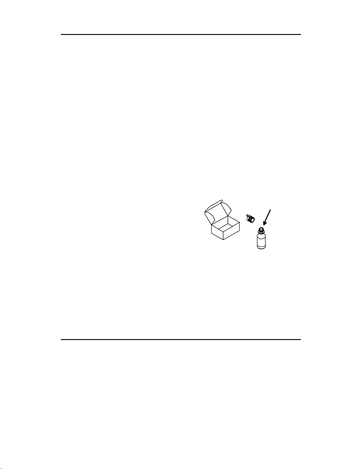
2-1.1. Preparation of the DO Electrolyte Solution
Unpack the 6562 DO Probe Kit. Locate the 5775 DO
Membrane Kit and prepare the electrolyte solution.
Dissolve the KCl (Potassium Chloride) in the dropper
bottle by filling it to the neck with deionized or distilled
water and shaking until the solids are fully dissolved.
After the KCl is dissolved, wait a few minutes until the
solution is free of bubbles before using.
2-1.2. Membrane Installation without the DO Probe Installed in the
Sonde
• Remove the protective cap and the dry membrane from the YSI 6562 DO Probe. Handle the
probe with care to prevent the sensor tip from becoming scratched or contaminated.
• Leave the protective cap in place over the connector end of the probe to prevent contamination
by the electrolyte.
A DD DI OR DIS T IL L E D
WATER
ADV6600 Y S I Environmental Page 5
Page 16
Section 2. Preparation of the Sonde
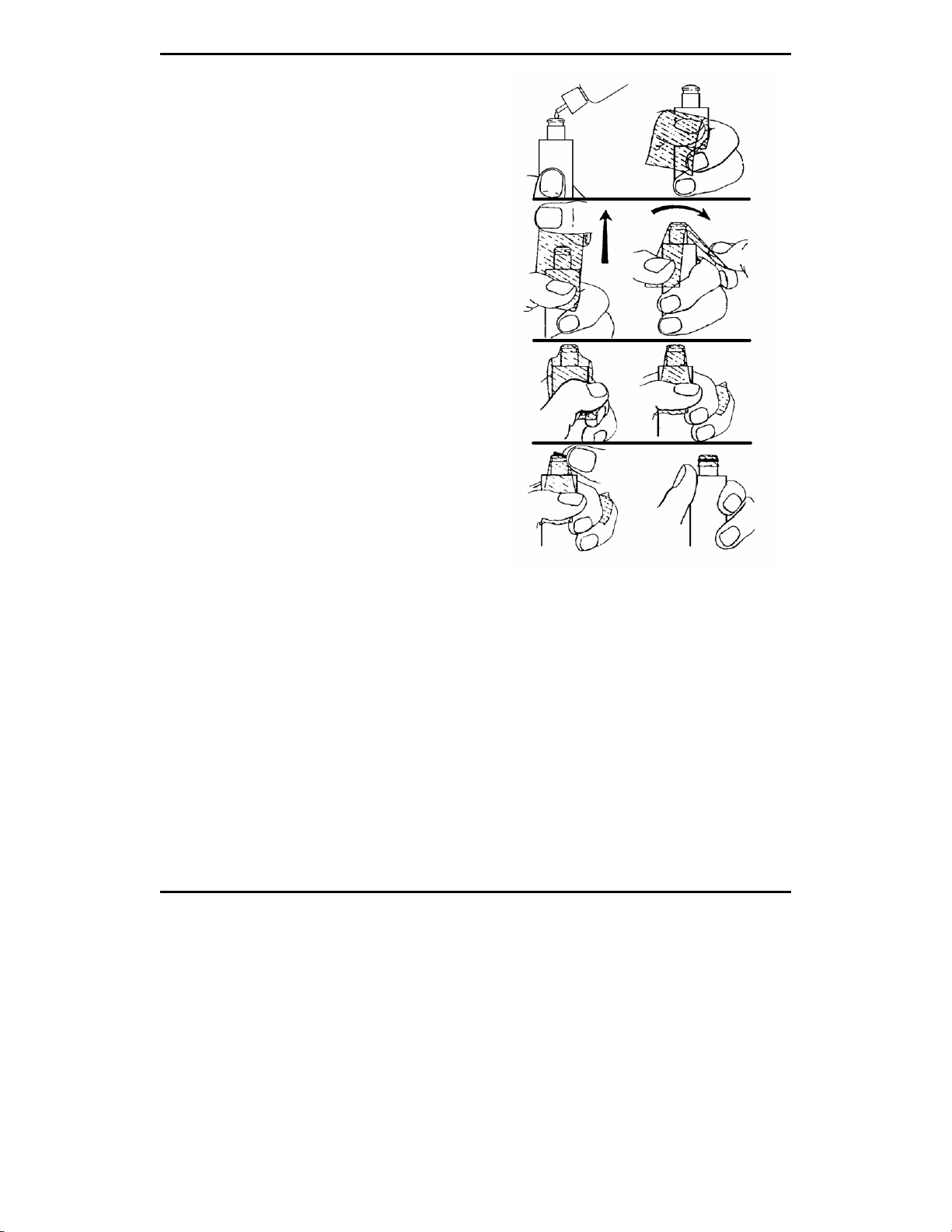
• Hold the probe in a vertical position and apply a
few drops of electrolyte solution to the tip. The
fluid should completely fill the small moat
around the electrodes and form a meniscus on
the tip of the sensor. Be sure no air bubbles are
visible. If necessary, shake off the electrolyte
and start over.
• Secure a membrane between your thumb and the
probe body. Always handle the membrane
with care, touching it only at the ends.
• With the thumb and forefinger of the opposite
hand, grasp the free end of the membrane. With
one continuous motion, gently stretch it up, over ,
and down the other side of the sensor. Do not
hesitate to stretch the membrane until it
conforms to the face of the sensor. Secure the
membrane with the forefinger of the hand
holding the probe body.
• Roll the o-ring over the end of the probe, being
careful not to touch the membrane surface with
your fingers. There should be no wrinkles or air
bubbles. If any are present, remove the
membrane and repeat the installation procedure
with a new membrane. Squeeze the o-ring every
90 degrees to equalize the tension. Do not use
grease or lubricant of any kind on the o-ring.
• Trim off any excess membrane with a sharp knife, a scalpel, or scissors. Make the cut about
1/8-inch below the o-ring. Rinse off any excess KCl solution, but be careful not to get any
water in the connector.
Note: You may find it more convenient to mount the probe vertically in a vise with rubber jaws
while applying the electrolyte and membranes to the sensor tip.
2-1.3. Membrane Installation with the DO Probe Installed in the
Sonde
• Secure the sonde in a vertical position using a vise, or a clamp with rubber jaws and ring stand.
Secure it tightly so that it will not move during membrane installation. Position the sonde with
the sensors upright. Remove the calibra tion cup or pr obe guard from t he sonde.
ADV6600 Y S I Environmental Page 6
Page 17

Section 2. Preparation of the Sonde
• Remove the old DO membrane and clean the probe tip with water and lens cleaning tissue.
Make sure to remove any debris or deposits from the O-ring groove. Handle the probe with
care to prevent the sensor tip from becoming scratched or contaminated.
• Apply a few drops of electrolyte solution to the tip of the probe. The fluid should completely
fill the small moat around the electrodes and form a meniscus on the tip of the sensor. Be sure
no air bubbles are visible. If necessary, shake off the electrolyte and start over.
• Hold the membrane so that all four corners are supported, but do not stretch the membrane
laterally. Always handle the membrane with care, touching it only at the ends.
• Position the membrane over the probe, keeping it parallel to the probe face.
• Using one continuous downward motion, stretch the membrane over the probe face. Do not
hesitate to stretch the membrane until it conforms to the face of the sensor.
ADV6600 Y S I Environmental Page 7
Page 18
Section 2. Preparation of the Sonde
• Roll the o-ring over the end of the probe, being careful not to touch the membrane surface with
your fingers. There should be no wrinkles or air bubbles. If any are present, remove the
membrane and repeat the installation procedure with a new membrane. Squeeze the o-ring
every 90 degrees to equalize the tension. Do not use grease or lubricant of any kind on the oring.
• Trim off any excess membrane with a sharp knife, a scalpel, or scissors. Make the cut about
1/8-inch below the o-ring. Rinse off any excess KCl solution.
• Use caution when replacing the prob e gua rd that you do not touch the membrane. If you
suspect that the membrane has been damaged, replace it immediately.
2-2. Installing Water Quality Probes
Remove the calibration/transport cup from your ADV6600 by hand to expose the bulkhead.
Note: The ADV probe is a non-removable sensor.
2-2.1. Removing the Port Plugs
Using the long extended end of the probe installation tool supplied in the YSI 6570 Maintenance
Kit, remove the port plugs by unscrewing them from the b ulkhead of the sonde. Save all the port
plugs for possible future use. If the provided tool is misplaced or lost, you may use 7/64” and 9/64”
hex keys as substitutes.
NOTE: You may need pliers to remove the ISE port plugs, but do not
probes. Hand-tighten only.
use pliers to tighten the ISE
ADV6600 Y S I Environmental Page 8
Page 19
Section 2. Preparation of the Sonde
V
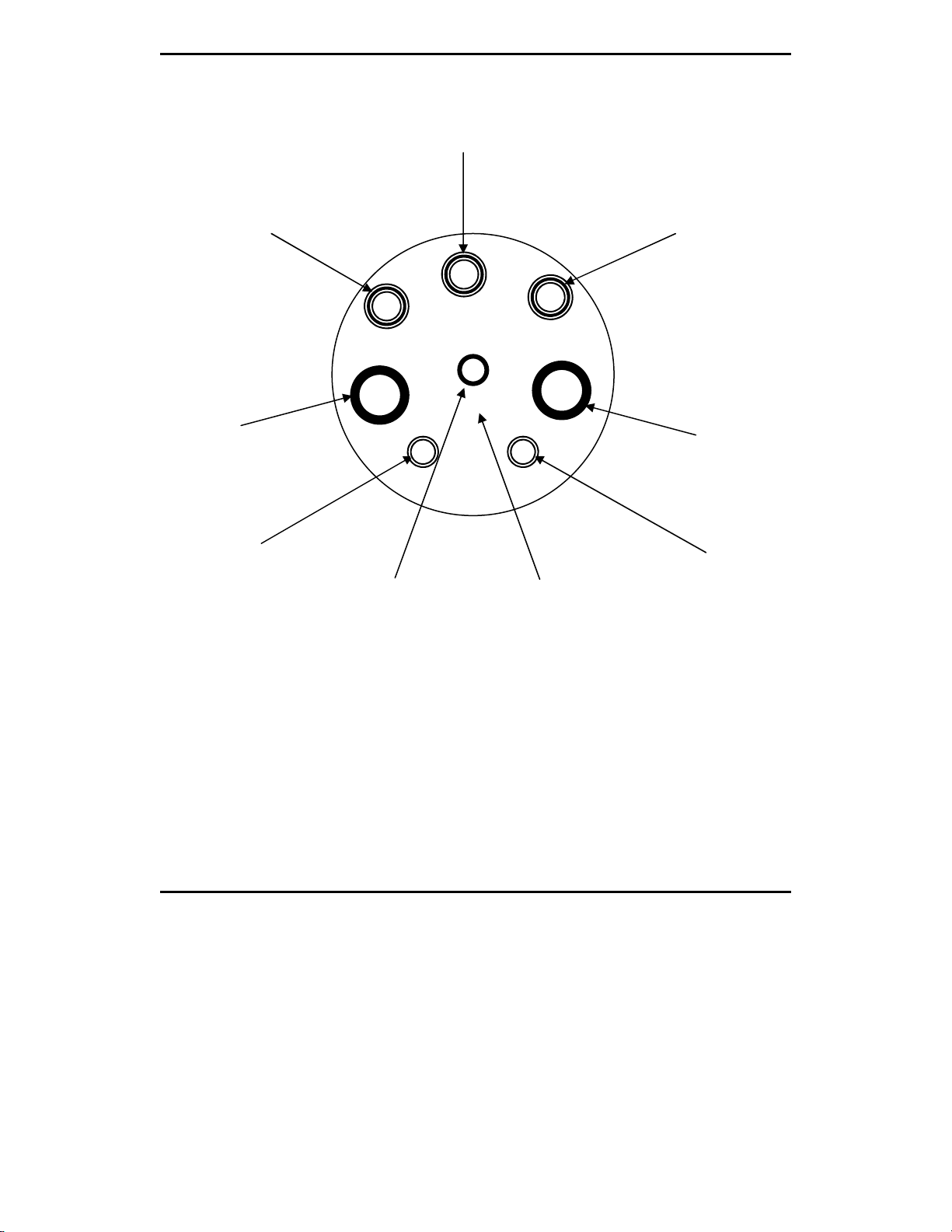
2-2.2. Bulkhead Diagram
Conductivity/Temperature
pH /ORP
º
Optical
ISE
AD
ADV Probe = Non-removable
Pressure Sensor = Non-removable
6562 Dissolved Oxygen (DO) probe = 3-pin connector
6560 Conductivity/Temperature = 6-pin connector
6561 pH probe = 4 pin connector
6565 Combination pH/ORP probe = 4 pin connector
6882 Chloride (ISE) Probe = leaf spring connector
6883 Ammonium (ISE) Probe = leaf spring connector
6884 Nitrate (ISE) Probe = leaf spring connector
6026 Turbidity (Optical) Probe, Wiping = 8 pin connector
6136 Turbidity (Optical) Probe, Wiping = 8 pin connector
6025 Chlorophyll (Optical) Probe, Wiping = 8 pin connector
6130 Rhodamine WT (Optical) Probe, Wiping = 8 pin connector
Pressure
DO
Optical
ISE
ADV6600 Y S I Environmental Page 9
Page 20

Section 2. Preparation of the Sonde
2-2.3. O-Ring Lubrication
Apply a very thin coat of o-ring lubricant, supplied in the YSI 6570 Maintenance Kit, to the o-rings
on the connector end of each probe to be installed. After application, the o-ring lubricant should not
be visible, but rather it will add a slight shine to the o-ring. If the lubricant can visibly be seen,
remove the excess very carefully with a piece of lens tissue (or equivalent non-shedding material,
i.e. fibreless q-tips), being careful not to get any on the probe connectors.
Caution! Make sure that there are no contaminants between the o-ring and the probe.
Contaminants that are present under the o-ring may cause the seal to leak when the sonde is
deployed.
2-2.4. Installing the Optical Probes
If you have a turbidity, chlorophyll, and/or rhodamine WT probe, it is recommended that the optical
sensors be installed first. If you are not installing one of these probes, do not remove the port plug,
and go on to the next probe installation.
Install the probe into the port, seating the pins of the two connectors before you begin to tighten.
Tighten the probe nut to the bulkhead using the short extended end of the tool supplied with the
probe. Do not over-tighten. Be careful not to cross-thread the probe nut.
The optical ports of the ADV6600 are labeled “T” and “C” on the sonde bulkhead. Each port can
accept any of the four optical sensors. Be sure to take note of which sensor is installed in which port
so that you will later be able to set up the sonde software correctly.
2-2.5. Installing the Conductivity/Temperature, DO, and pH/ORP
Probes
Insert the probe into the proper port using the diagram on the previous page as a guide and rotate the
probe until the pins engage. Seat the pins of the two connectors together as far as possible before
you begin to tighten.
The probes are held in place with slip nuts. With the connectors aligned and the two connector
halves engaged, hand-tighten the probe nut and then use the long extended end of the probe
installation tool to snug it. Do not over-tighten. Be careful not to cross-thread the probe nuts.
2-2.6. Installing the ISE Probes
The ammonium, nitrate, and chloride ISE probes do not
without tools. Use only your fingers to tighten. Make sure that the probe body of the ISE probes is
seated directly on the sonde bulkhead. This will ensure that connector seals will not allow leakage.
have slip nuts and should be installed
ADV6600 Y S I Environmental Page 10
Page 21

Section 2. Preparation of the Sonde
Any ISE probe can be installed in either of the two ports labeled “3” or “4” on the sonde bulkhead.
Be sure to take note of which sensor was installed in which po rt so that you will later be able to set
up the sonde software correctly.
2-2.7. Installing the Probe Guard
Included with your sonde is a probe guard. The probe guard protects the probes during calibration
and measurement procedures. Once the probes are installed, the guard can be installed by aligning it
with the threads on the bulkhead and turn the guard clockwise until secure. Be sure not to damage
the DO membrane during installation of the probe guard.
2-3. Attaching Your Sonde to a Computer
2-3.1. Installing the Batteries
The ADV6600 utilizes 8 C-size alkaline batteries which were supplied with the instrument. These
batteries are not rechargeable and should be properly disposed of when expended.
Install the batteries into the ADV6600 according to the following directions:
1. Loosen the battery lid screws. If necessary, a flathead screwdriver may be used. It can be
helpful to press the battery lid while unscrewing retaining thumb screws such that the lid or
thumb screws do not bind.
2. Remove the battery lid and install the batteries, as
shown. Observe the correct polarity noted on the
outside of the battery lid before inserting each
battery into the battery chamber.
3. Check the O-ring and sealing surfaces for any
contaminates which could interfere with the O-ring
seal of the bat t ery cham b e r . Remove any
contaminates present.
4. Return the b a tt ery lid an d ti g hten the sc r ews by
hand. It can be helpful to apply some pressure to
the battery lid while screwing the thumb screws to
prevent binding or non-uniform compression.
Note: Always power the system off when not in use to avoid draining the system batteries.
ADV6600 Y S I Environmental Page 11
Page 22

Section 2. Preparation of the Sonde
2-3.2. Preparing the Cable
The cable purchased with your ADV6600 has an Impulse
ADV6600 end and a military-style 8 pin connector (MS-8) on the interface end. Before
communicating with the ADV6600 through this cable, the YSI 6095B MS-8 to DB-9 adapter
(supplied with each sonde) must be connected to the MS-8 end of the cable. Place the MS-8 ends
of the cable and adapter together, and rotate until the alignment pins engage and the male and
female portions of the connector slide together. Once the bodies of the connectors are fully
engaged, twist the knurled ring on the cable until the two pieces lock together.
TM
MCIL-8-MP connector on the
2-3.3. Using the AC Power Supply
Although the ADV6600 has internal batteries, using the optional Model 6651 power supply for
laboratory studies and for sonde calibration and setup is often convenient and extends battery life.
The 6651 will automatically convert line voltages of 90 to 264 to 12 VDC and allows for the use of
line input cords from most countries world-wide. The 6651 is supplied with an American/Canadian
cord.
To use the 6651, attach the four-pin connector from the power supply to the mating connector on the
6095B adapter by twisting them together and then simply plug the power cord into the appropriate
AC outlet. Once the power and communications cable has been powered, be sure that the exposed
8-pin connector does not come in contact with water, metal, or other shorting material as this can
cause permanent and irreversible damage to the connector.
ADV6600 Y S I Environmental Page 12
Page 23
Section 2. Preparation of the Sonde
Y
Y
Y
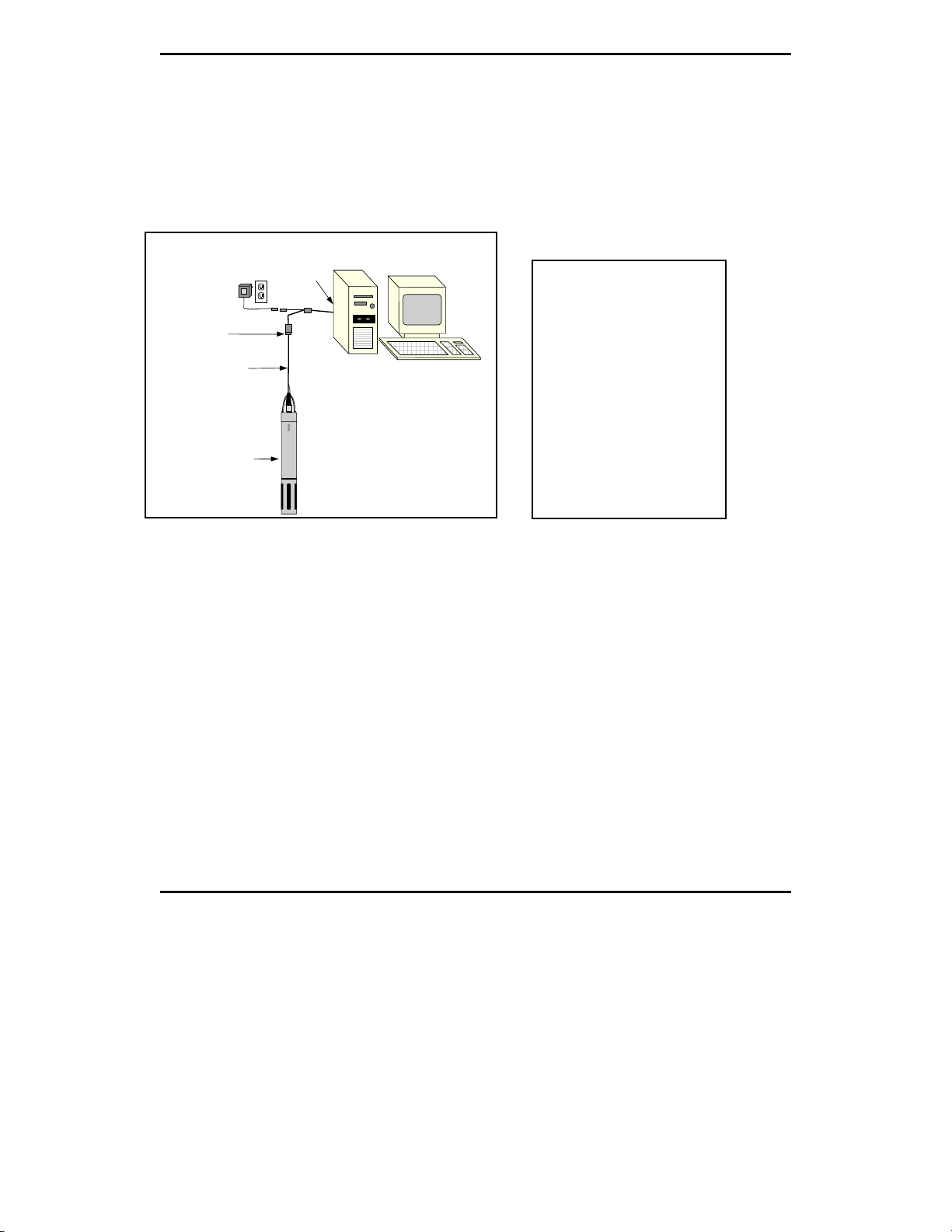
2-3.4. Attaching the Cable
Attach your ADV6600 to a computer for initial setup by connecting the proper end of the cable to
the sonde connector and attaching the strain relief connector to the sonde bail. Then connect the
other end of the cable assembly (DB-9) to a serial port on your computer. Use the diagram and
picture below to make sure that your connections are correct.
Power Supply*
MS-8
Sonde to Computer
DB-9
6095B
Adapter
Field Cable
ou will need...
❑
+
+
--
S
S
I
I
69
69
Sonde
Not required if you use
*
sonde battery
20
20
Now that the Water Quality sensors, power source, and cable have been installed on your
ADV6600, you are ready to proceed to installation of ADVantage 6600 PC software and the setup
of the firmware which resides within the sonde. These activities are detailed in Section 3.
Sonde
❑
Field Cable
❑
Computer with Com Port
❑
6095B MS-8/DB-9 Adapter
❑
605389 Power Supply *
ADV6600 Y S I Environmental Page 13
Page 24

Page 25

Section 3. Configuring Your ADV6600 –
Installation of ADVantage 6600 Software and
Sonde Firmware Set-up
In Section 2, you set up the physical components of your ADV6600 – sensors, power source, and
cable. In this section, you will learn how to install the PC software which allows interface to your
ADV6600 and how to use this interface to correctly configure the firmware packages in the sonde
which control the velocity and water quality sensors.
3-1. ADVantage 6600 Software – System Requirements
• IBM Compatible PC with Pentium processor or above
• Windows
• 32 MB memory
• 5 MB available disk space
• CD-ROM Drive
• RS-232 Serial Port
• Monitor capable of 800 x 600 resolution or better
3-2. Installing ADVantage 6600 Software
To install ADVantage 6600 software to your computer, perform the following steps:
• Place the ADVantage 6600 CD-ROM into the CD drive of your computer.
• Use Windows Explorer or My Computer to view files on the CD-ROM. Doub l e-click on
The display will indicate that ADVantage 6600 is proceeding with the setup routine. Follow the
instructions on the screen as the installation proceeds. For most applications, the default settings
should work without problems. After installation, there is no need to restart the computer.
3-3. Launching the Software
To run ADVantage 6600, click on the Windows Start button. Go to Programs>YSI
Software>ADVantage 6600; or click on the icon located on your desktop.
The program will display the following screen.
®
98, NT, 2000, ME, or XP
the ADVantage 6600_setup.exe file.
ADV6600 Y S I Environmental Page 15
Page 26
Section 3. Installation and Setup
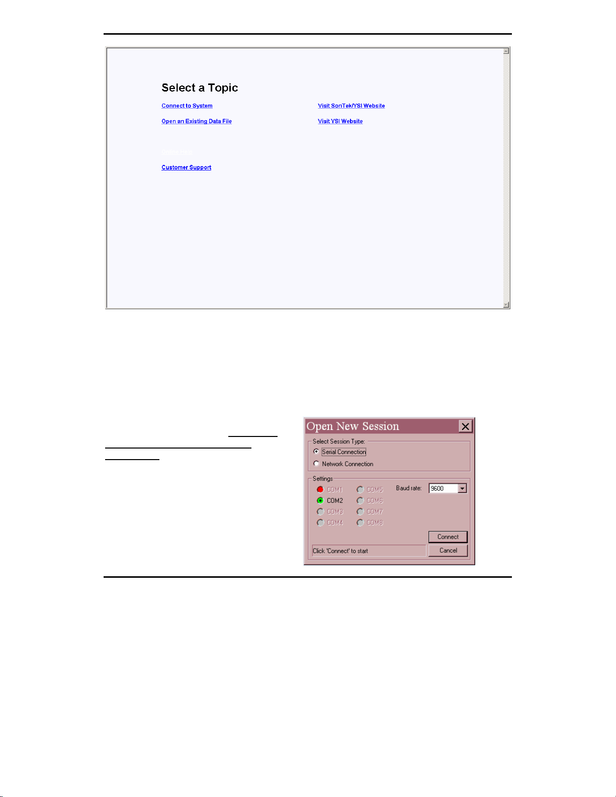
3-4. Connecting to the System
When choosing the “Connect to System” selection, the Open New Session dialog box will appear
as shown below. A Session is used to describe a mode in which the software will be utilized. The
type of session may be selected by clicking on the appropriate button.
The default settings in the dialog box establish a Serial Connection which allows direct connection
between the ADV6600 and your computer
through a serial (COM) port. This option
should be used for most ADV6600
applications. You will need to select the
COM port to which your ADV6600 is
attached and confirm that the baud rate is set
to 9600.
Settings
This area displays the available COM ports on
your computer and the COM port being used
ADV6600 Y S I Environmental Page 16
Page 27
Section 3. Installation and Setup
for the current session. There are a maximum of eight available COM ports.
The COM port radio buttons (labeled COM1 through COM8) will display in one of three colors –
green = available for use by an instrument; red = in use or not available for use by an instrument;
gray = not detected on the computer. Additionally, the “active” radio button (the one with a black
dot in the middle) shows which COM port is connected to th e instrument being used by the
currently selected session.
If no radio button is “active” for the selected session, you can click on the appropriate COM port
radio button to connect to the instrument via ADVantage 6600 software.
Baud Rate
This dropdown list lets you change the communications baud rate of your instrument for special
applications. The default baud rate is set to 9600 at the factory and this setting should be used for
all typical ADV6600 applications. The baud rate should NOT be changed from 9600 except on
advice from YSI Technical Support personnel.
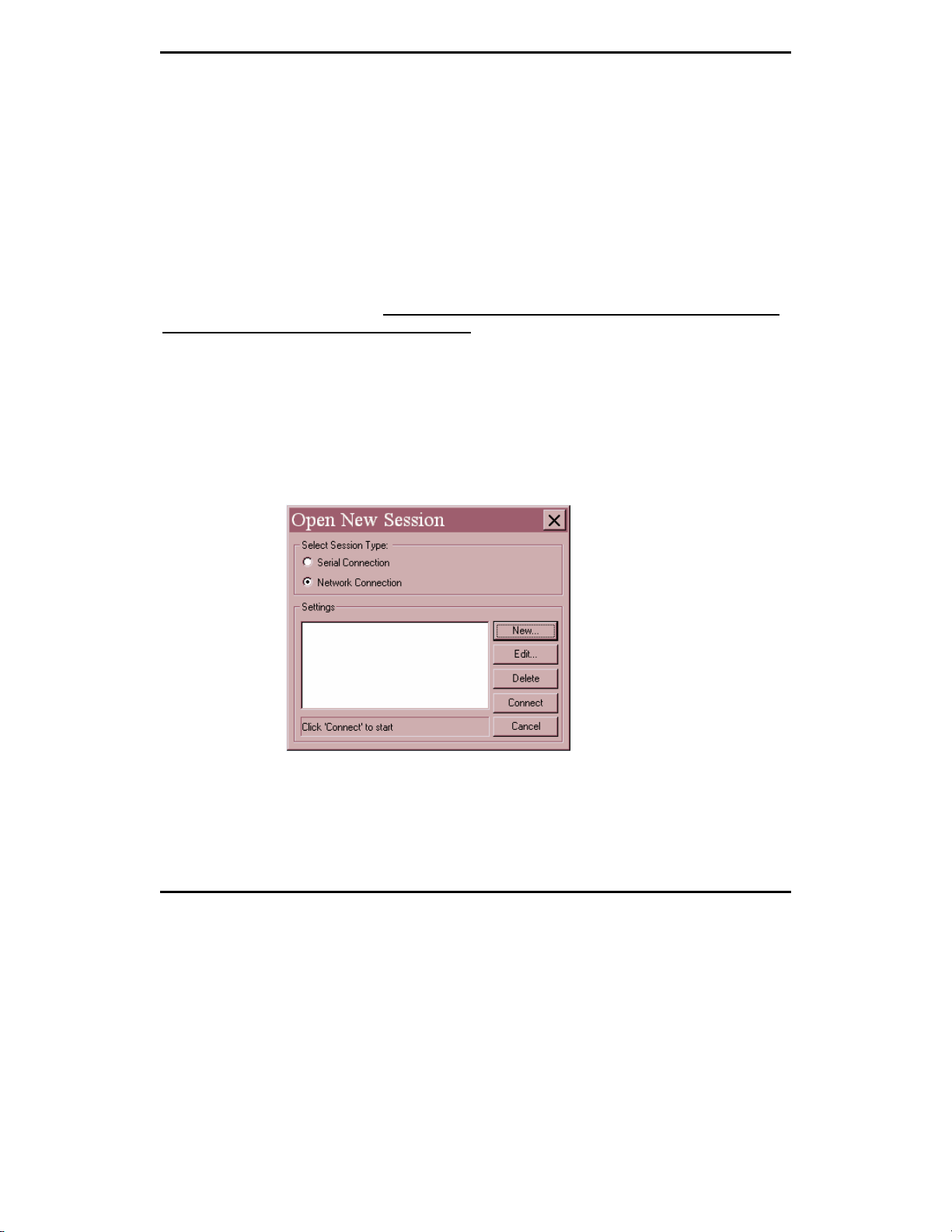
You may also select the Network Connection option by clicking the appropriate button and the
following dialog box will be shown. This option is for connections established through SonTek’s
SonGate software. A network (TCP/IP or LAN) must be in place and the host computer must be
running for this option to be used. When a network connection is chosen, the user will have the
option to select an existing network connection setup, create a new setup, or edit an existing setup
using the buttons on the right of the dialog box. When the setup information is entered and selected,
click on Connect to display the options for communicating with the instrument
.
REMEMBER: Unless advised o therwise by YSI Technical Support personnel, use the Serial
Connection option at a baud rate of 9600 to interface to your ADV6600.
ADV6600 Y S I Environmental Page 17
Page 28
Section 3. Installation and Setup
3-5. Understanding the Firmware of the ADV6600
There are three sets of software being utilized when working with the ADV6600. The ADVantage
6600 interface software which was just installed resides in your PC. The other two software
packages reside within the ADV6600 itself and are termed firmware
called “ADV Firmware” in this manual is designated as the “Master” of the two firmware
components and controls the ADV, compass/tilt, and pressure sensors as well as the lo gging and
data retrieval functions. The other firmware (called the “Water Quality Firmware” in this manual) is
designated as the “Slave” and controls only the water quality sensors
When communication is established with the ADV6600 from ADVantage 6600, the PC-based
software begins direct communication with the ADV firmware. If information is required from the
water quality sensors, the ADV firmware communicates in turn with the Water Quality firmware to
retrieve the data. Prior to using your ADV6600 in field studies it is necessary to set up both the
ADV and Water Quality firmware packages to provide the output appropriate to your studies and
this procedure is described in the following two sections.
. One firmware package is
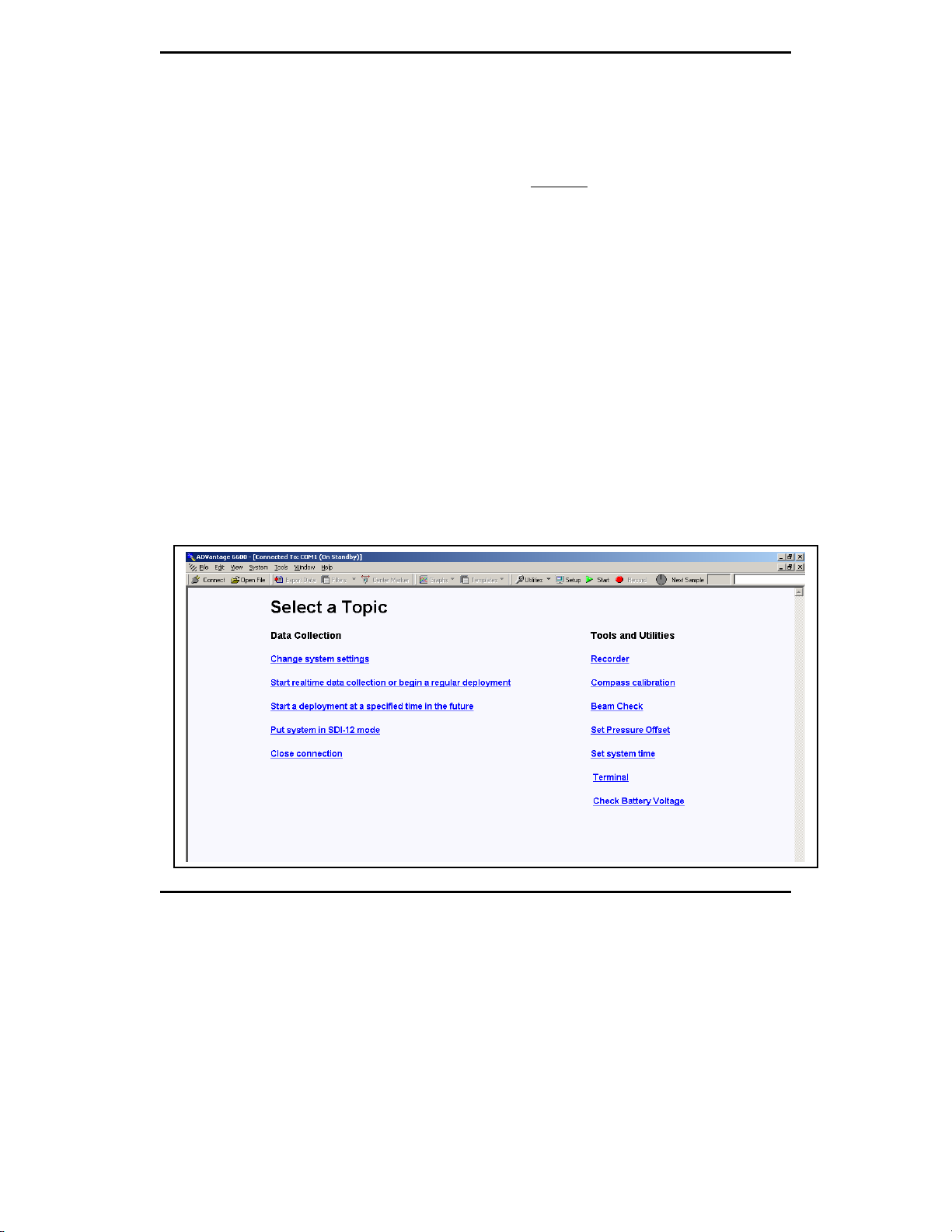
3-6. Setting up the Water Quality Sensor Firmware
3-6.1. Setting Up the Water Quality Sensors
After connecting to the system and opening a new session, the following screen will appear:
ADV6600 Y S I Environmental Page 18
Page 29
Section 3. Installation and Setup
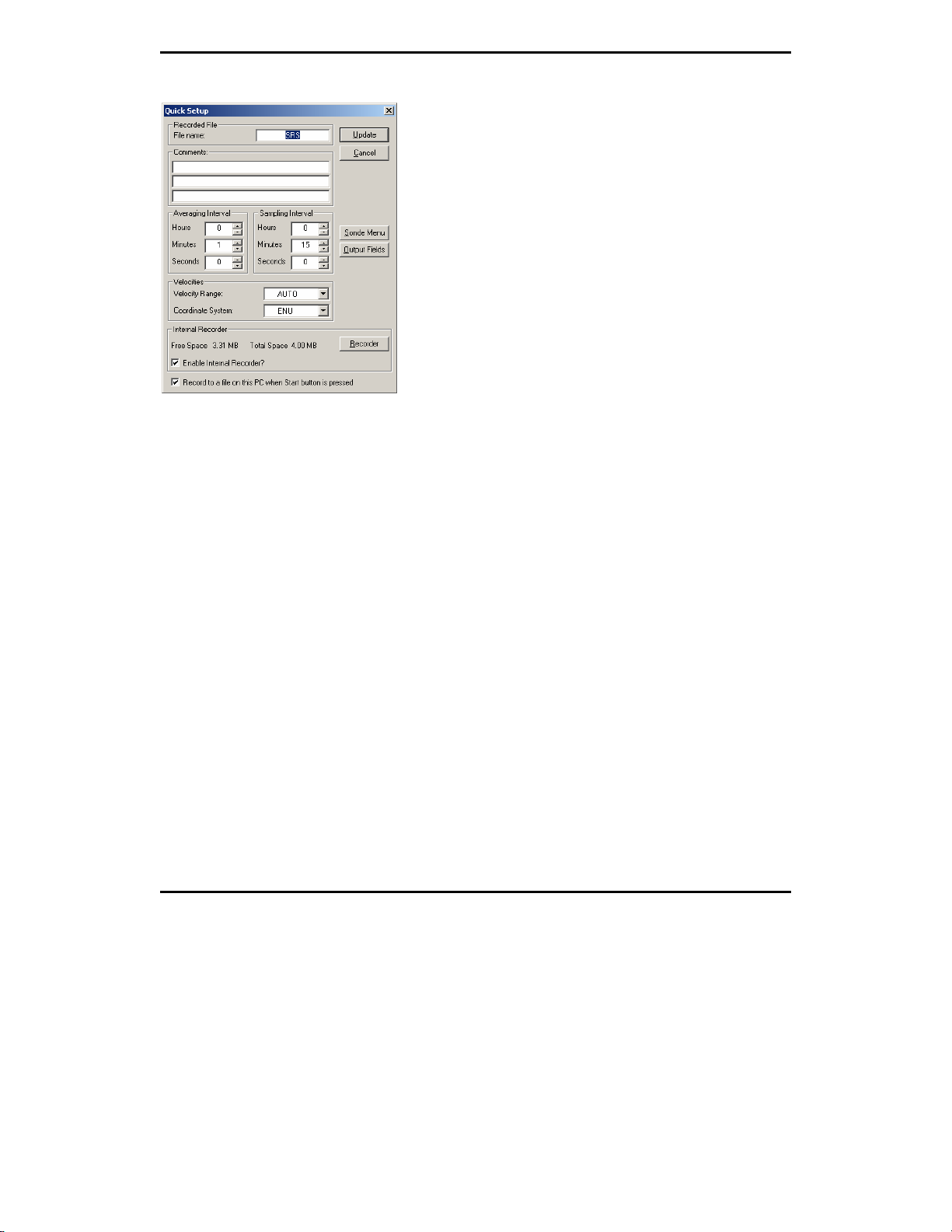
Select Change System Settings to display the Quick Setup dialog box as shown below.
Click on Sonde Menu to open a dialog window so that selections specific to the water quality
sensors can be viewed as shown below.
The water quality sensor items are selected by typing their corresponding number (e.g., 1 for
Calibrate). It is not necessary to press Enter to confirm a selection. When moving between menus
within the sonde software structure, use the 0 or Esc to back up to the previous menu. It is possible
to display the sonde command line (#) by pressing 0 or Esc until the question “Exit menu (Y/N)?”
ADV6600 Y S I Environmental Page 19
Page 30

Section 3. Installation and Setup
appears and then typing Y. To return to the Main menu of the sonde menu, type Menu after the “#”
and press Enter. The command line function may be useful during troubles hooting discussions
with YSI Technical Support personnel.
To save power, the Water Quality hardware will power down automatically if no interaction from
the keyboard occurs for approximately 60 seconds. When the firmware is in this “sleep” mode, the
first subsequent keystroke simply “wakes it up” and has no visible effect on the display. The next
keystroke after the unit is “awakened” will be input to the firmware in the intended manner. Thus,
if you press a key after the sonde has been inactive for some time and receive no response, press the
key again.
3-6.2. Water Quality Menu Flowchart
Several menu functions available on previous YSI sondes are no longer available on the ADV6600.
Due to the master-slave relationship between the ADV and the Water Quality hardware packages,
accessibility to these functions was removed, preventing interruption of communications bet ween
the firmware of each component.
SONDE MENU
ADV6600
1. Conductivity
1. Calibrate
2. Report
3. Sensor
4. Advanced
1. (
) Time
2. (
) Temperature
3. (
) Conductivity
▼ MORE ▼
2. Dissolved Oxy
3. ISE1 pH
▼ MORE ▼
1. (
) Date
2. (
) Time hh : mm : ss
3. (
) Temp C
▼ MORE ▼
1. Cal constants
2. Setup
3. Sensor
ADV6600 Y S I Environmental Page 20
Page 31

Section 3. Installation and Setup
3-6.3. Setting Up Installed Sensors
To activate the water
quality sensors that are
installed in the
ADV6600, select 3-
Sensor from the Sonde
Main menu. The
Sensor menu allows
you to Enable or
Disable (turn on or off)
any available sensor
and, in some cases, to
select the port in which
your sensor is installed.
Enter the corresponding number or letter to enable the sensors that are installed on your sonde. An
asterisk indicates that the sensor is enabled.
When selecting ISE3, ISE4, or any of the Optical ports, a submenu will appear. When this occurs,
make certain the sensor selected corresponds to the port in which the sensor is physically installed .
Note:
• Only ORP can be enabled as ISE2.
• ISE ports 3 and 4 can have one of three probes (nitrate, ammonium, or chloride) installed as
indicated by the submenus.
• Each optical port can have one of four probes (6026 turbidity, 6136 turbidity, chlorophyll, or
rhodamine WT) installed as indicated by the submenus.
• Only one probe of any type can be installed and activated in the ADV6600 sonde. For example,
it is not possible to use chlorophyll probes in both the Optic T and Optic C ports. However, it is
possible to use both the 6026 and the 6136 turbidity probes simultaneously
After all installed sensors have been enabled, press Esc or 0 to return to the Main Menu.
3-6.4. Setting Up Reports
The Report menu allows you to select the parameters and units of measure that will be output from
the Water Quality sensors and eventually be available for display in the ADVantage 6600 software.
Select 2-Report from the sonde Main menu. The menu below, or a similar menu
The parameters listed will depend on the sensors available and enabled on your sonde.
, will be displayed.
ADV6600 Y S I Environmental Page 21
Page 32

Section 3. Installation and Setup
The asterisks (*) that follow the numbers or letters indicate that the parameter will appear on all
outputs and reports. To turn a parameter on or off, type the number or letter that corresponds to the
parameter.
For parameters with multiple unit options such as temperature, conductivity, specific conductance,
resistivity and TDS, a submenu will appear as shown, allowing selection of desired units for this
parameter.
After configuring your instrument with the desired parameters, press Esc or 0 to return to the Main
menu.
Please note the following:
• Even if all of the Water Quality sensors available on the ADV6600 are enabled, the
measurements for those sensors will not appear on your display unless the parameter is
selected in Report setup.
• Only the exact Report parameters and their selected units as selected in Report will be
logged to internal memory during logging studies and you will NOT be able to obtain
ADV6600 Y S I Environmental Page 22
Page 33

Section 3. Installation and Setup
calculated parameters after the fact. For example, if you want to log specific conductance
during an unattended study, it MUST be active in the Report at the time the study is begun.
If only conductivity is active in the report, it will NOT be possible to automatically convert
the readings to specific conductance at a later time with ADVantage 6600 software.
The following table provides a complete listing of the abbreviations utilized for the various
parameters and units available in the Report setup menu.
Parameter Description
Date Day/Month/Year (format selectable)
Time Hour:Minute:Second (24-hour clock format)
Temp C Temperature in degrees Celsius
Temp F Temperature in degrees Fahrenheit
Temp K Temperature in degrees Kelvin
SpCond mS/cm Specific Conductance in milliSiemens per centimeter
SpCond uS/cm Specific Conductance in microSiemens per centimeter
Cond mS/cm Conductivity in milliSiemens per centimeter
Cond uS/cm Co nductivity i n microSiemens per centimeter
Resist MOhm*c m Resistivity in MegaOhms * centimete r
Resist Kohm*cm Resistivity in KiloOhms * centimeter
Resist Ohm*cm Resi stivity in Ohms * centi meter
TDS g/L Total dissolved solids in grams per liter
TDS kg/L Total dissolved solids in kilograms per liter
Sal ppt Salinit y in parts per thousand (set to local barometer at
calibration)
DO sat % Dissolved oxyge n in % air saturation
DO mg/L Dissolved oxygen in milligra ms per liter
DO chg Dissolved oxygen sensor charge
pH pH in standard units
pH mV millivolts associated with the pH reading
ORP mV Oxidation reduction potential value in millivolts
NH4+ N mg/L Ammonium Nitroge n i n milligrams/liter
NH4+ N mV Ammonium Nitrogen in millivolt reading
NH3 N mg/L Ammonia Nitrogen in milligrams/liter
NO3- N mg/L Nitrate Nitrogen in milligrams/liter
NO3- N mV Nitrate Nitrogen in millivolt reading
Cl- mg/L Chloride in milligrams/liter
Cl- mV Chloride in millivolt reading
Turbid NTU Turbidity in nephelometric turbidity units from 6026 sensor
Turbid+ NTU Turbidity in nephelometric turbidity units from 6136 sensor
Chl ug/L Chlorophyll in micrograms/liter
Fluor %FS Fluorescence in percent Full Scale
Rhod ug/L Rhodamine WT in micrograms/liter
ADV6600 Y S I Environmental Page 23
Page 34

Section 3. Installation and Setup
DOsat % Local Dissolved oxygen in % air saturation (set to 100 % at
calibration)
3-6.5. Advanced Menu Features
From the Sonde Main menu select 4-Advanced to display the sensor calibration constants,
additional setup options, and sensor coefficients/co nstants as shown below. The parameters listed
will depend on the sensors installed and enabled.
Select 1-Cal constants to display the calibration constants. Note that values only appear for the
enabled
relative to the calibration constants. Error messages will appear during calibration if values are
outside the indicated operating range unless the designation is “not checked”.
sensors. The following table provides the default value, operating range, and comments
Parameter Default Operating Range Comments
Cond 5 4 to 6 Traditional cell constant
DO Gain 1
ORP offset mV
pH offset 0.0 -400 to 400
pH gain -5.0583 -6.07 to -4.22
NH4 J 51.2 Not checked
NH4 S 0.195 0.15 to 0.217
NH4 A 1.092 Not checked
NO3 J 99.5 Not checked
NO3 S -0.195 -0.217 to -0.15
ADV6600 Y S I Environmental Page 24
0.0 -100 to 100
0.5 to 2.0
Page 35

Section 3. Installation and Setup
Parameter Default Operating Range Comments
NO3 A 2.543 Not checked
Cl J 99.5 Not checked
Cl S -0.195 -0.217 to -0.15
Cl A 2.543 Not checked
Turb Offset 0 -10 to 10
Turb A1 500
Turb M1 500
Turb A2 1000
Turb M2 1000
Chl Offset 0 -30 to 20
Chl A1 500
Chl M1 500
Chl A2 1000
Chl M2 1000
Rhod Offset 0 -10 to 10
Rhod A1 500
Rhod M1 500
Rhod A2 1000
Rhod M2 1000
0.6 to 1.5
0.6 to 1.5
0.6 to 1.5
0.6 to 1.5
0.6 to 1.5
0.6 to 1.5
Range is ratio of M1 to A1
Range is ratio of (M2-M1) to
(A2-A1)
Range is ratio of M1 to A1
Range is ratio of (M2-M1) to
(A2-A1)
Range is ratio of M1 to A1
Range is ratio of (M2-M1) to
(A2-A1)
From the Advanced menu, select 2-Setup to activate or deactivate Auto sleep RS-232. Activation
of this feature enables a power savings system within the sonde. When enabled, power is only
applied to the sensors during sampling or calibration. The most important aspect of this feature is
its effect on the dissolved oxygen protocol. For this reason, the feature should be activated for most
applications. The selection should only be deactivated if you are running spot sampling studies
where the Averaging Interval and Sample Interval are set to the same value (see later).
From the Advanced menu, select 3-Sensor to display and change user-configurable consta nts as
shown. Select the appropriate number to view these parameters.
ADV6600 Y S I Environmental Page 25
Page 36

Section 3. Installation and Setup
The number of items on this menu depends on the sensors that are available and enabled on your
sonde. Below we describe every possible item on this menu. Your sonde may not
have every item described.
NOTE: The user is cautioned to retain the default settings unless advised to change them by YSI
Technical Support. Changes should only be necessary for special applications.
TDS constant
Default: 0.65
Salinity
Default: 0
Pres psi
Default: 0
DO temp co %/C
Default: 1.1
DO warm up sec
Default: 60
Wipes
Default: 1
This selection allows you to set the constant used to calculate TDS. TDS
in g/L is calculated by multiplying this constant times the sp ecific
conductance in mS/cm. This item will only appear if the conductivity
sensor is enabled in the “Sensors enabled” menu.
This selection allows you to input a manually-acquired value of salinity
for calculating DO mg/L. This item is not used or displayed if the
conductivity sensor
This selection allows you to set a value of pressure for calculating other
parameters like salinity.
This selection allows a user to input the dissolved oxygen temperature
coefficient. Do not change this value unless you consult YSI Technical
Support. This item will only appear if the DO sensor is enabled in the
Sensors menu.
This selection allows a user to change the warm up period for the
dissolved oxygen sensor. This setting should always be equal to the
averaging interval established in the Quick Setup dialog box.
This selection will determine the number of cleaning cycles that will
occur when an optical probe wiper is activated manually or
is enabled in the Sensors menu.
ADV6600 Y S I Environmental Page 26
Page 37

Section 3. Installation and Setup
automatically. The wiper functions bi-directionally. A selection of “1”
results in three passes of the wiper over the optical face, twice in one
direction and once in the reverse direction. In most applications, a single
cleaning cycle is adequate to keep the optical surface free of bubbles and
fouling. However, in particularly harsh enviro nments addit ional cleaning
cycles may be needed. This item will only appear if a turbidity,
chlorophyll, or rhodamine WT sensor is enabled in the Sensor menu.
Wipe interval
Default: 1
SDI12-M/wipe
Default: 1
Turb temp co %/C
6026 Default: 0.3
6136 Default: 0.6
(* ) TurbSpike Filter W hen this ite m is activated, the output of the turbidity sensor is
In applications where the instrument is collecting data in SDI-12
communication mode, the wiper mechanism of the probe should be
activated automatically in a periodic manner to clean the optical surface
for fouling and bubbles. The value entered at this selection is the number
of minutes between each automatic cleaning cycle. Thus, if Wipe Int is
set to “5” and the instrument is in the Run mode, the wiper will activate
every 5 minutes with no manual input. This item will only appear if a
turbidity, chlorophyll, or rhodamine WT sensor is enabled in the Sensors
menu.
The value of Wipe Int is sometimes overridden when the instrument is
set up in the Unattended sampling mode. Under these conditions, the
wiper will be automatically activated at the interval assigned in the
Unattended setup rather than that assigned in Wipe Int. Thus, in an
Unattended study setup at a 15 minute sampling interval, the wiper will
be activated only once every 15 minutes rather than at the indicated Wipe
Int of 1 minute.
CAUTION: If Wipe Int is set to zero, then no wiping will occur either in
Discrete or Unattended Sampling. Make certain that Wipe Int is set to
some finite value prior to setting up an Unattended study or no automatic
cleaning will occur.
This is the number of wiping cycles when the sonde is in SDI12 mode.
The wiper will automatically wipe each time this many SDI12 “M”
commands have been issued. If this value is set to zero, then no
automatic wiping will occur. This item will only appear if a turbidity,
chlorophyll, or rhodamine WT sensor is enabled in the Sensors menu.
This entry sets the coefficient for the temperature compensation of
turbidity readings from the 6026 and 6136 sensors. The default values
should not be changed by the user without consulti ng YSI Technical
Support. This item will only appear if a turbidity sensor is enabled in the
Sensor menu.
ADV6600 Y S I Environmental Page 27
Page 38

Section 3. Installation and Setup
mathematically processed to minimize the effect of unusual (or “bad”)
readings on the overall data presentation. In most cases, these “spike”
events are the result of the chance passage of large suspended particles
across the probe optics just at the time a reading is taken. Activation of
this option generally results in a better display of the “average” turbidity
of the water under examination and its use is recommended for most
sampling and unattended applications. This item will only appear if a
turbidity sensor is enabled in the Sensors menu.
Chl temp co %/C
Default: 0.0
This entry sets the coefficient for the temperature compensation of
chlorophyll readings from the 6025 sensor. The default value of zero
should only be changed by the user after establishing the temperature
compensation factor for the phytoplankton sample in question. This item
will only appear if a chlorophyll sensor is enabled in the Sensors menu.
3-7. Setting up the ADV Sensor Firmware
The ADV firmware controls the velocity, pressure, and compass/tilt sensors. In addition, the real
time clock which controls the overall ADV6600 system and is recorded with each data string, is part
of the ADV firmware. Prior to using your ADV6600 in field studies, you must set the real time
clock and customize your ADV parameter output as described in the sections below.
3-7.1. Setting the System Time
When establishing a connection to the ADV6600 for the first time from a new PC or laptop, it is
advisable to set the time of the instrument. First, verify that the time shown on your computer is
correct. Next, connect to the ADV6600 and open a new session. Under the Tools and Utilities
screen options, select Set system time. The time in the ADV6600 will automatically be reset to
match the time of the computer it is connected to.
3-7.2. Setting Up the ADV Parameter Output
The ADV parameter output format can be configured from the Quick Setup dialog box which is
accessed by clicking the Change System Settings selection under the Data Collection screen menu.
A typical Quick Setup box is shown below. To show a list of ADV parameters, click on the Output
Fields selection as shown below.
ADV6600 Y S I Environmental Page 28
Page 39

Section 3. Installation and Setup
Under most circumstances, the user is advised to make sure that all of the items in the Fields listing
are active, i.e., a check mark appears in all boxes. Outputting all parameters to the PC during real
time studies and to the ADV6600 internal memory during unattended monitoring studies will allow
the full capability of the ADV6600 system to be realized. If the user does not want to view some of
the information in reports and plots, parameter outputs can easily be “masked” using the
ADVantage 6600 software package, but still retained in the data files for use in later data analysis.
Therefore, YSI strongly recommends that all fields be left active for studies where the data is stored
to a PC or internal memory. The selection is present primarily to limit the ADV6600 output for
SDI-12 studies as described in Section 6.3. However, there may be unusual circumstances in non
SDI-12 studies where the user will want to eliminate some of the ADV parameters and this can be
accomplished by clicking on the boxes to remove the check mark.
Note that many of the ADV parameters have subparameters bundled within the same item. For
example, the velocity parameter contains three separate outputs (V
, VN, and VU) which represent
E
the velocity in the “East”, “North”, and “Up” directions relative to the earth coordinate system (and
are derived using the velocity from the ADV and internal compass). Detailed descriptions of the
parameters listed in the Fields dialog box are provided in the table below.
Sample Number Sequential numbers (incremented by one unit) starting with “1” which
are incremented by one unit and are displayed and/or logged time a
sample is taken.
Time The date and time stamps which are displayed and/or logged with each
set of data points.
Speed and Direction The speed and direction of the water.
Vel The three components of water velocity (East, North, Up)
Vel Std Dev The Standard Deviation of the water velocity
ADV6600 Y S I Environmental Page 29
Page 40

Section 3. Installation and Setup
Amplitude The level of returned signal based on the concentration and/or particle
size found in the water.
Compass The heading, pitch, and roll data from the compass which is applied to
the raw velocity data to convert it to East, North, Up components.
Temperature The output of the temperature sensor associated with the ADV sensor.
The output is reported as “ADV Temperature”. Note that there is also a
temperature parameter associated with the Water Quality sensors which
will be similar, but probably not identical, to the “ADV Temperature”
due to differences in location and time constants.
Pressure The reading of the ADV6600 pressure sensor which can be translated
into depth of water value.
Battery Voltage The voltage associated with the internal C-cells of the ADV6600 or
external power source (whichever is greater).
Boundary Range The range from the tip of the ADV (transmitter) to the closest boundar y
(i.e. the bottom of a stream) if within detectable range (varies depending
on angle and material type). The value is reported as a -1 if not detected
or is out of range.
Water Quality Data The water quality parameters which are active in the Report setup.
3-8. Exiting the ADV6600 Firmware
When you have finished setting up the ADV6600 firmware, be sure to close ADVantage 6600
completely by clicking the “x” in the upper right hand corner of the window. You will see the
following message:
Under virtually all circumstances, you will want to click the “Yes” selection so that the ADV6600
will power down to its idle mode in order to save power.
3-9. ADV6600 Firmware Upgrades
ADV6600 Y S I Environmental Page 30
Page 41

Section 3. Installation and Setup
Periodically, YSI will make improvements and modifications to the firmware residing in an
instrument. It is recommended that you periodically check for updated firmware for the ADV6600
on the YSI website at www.ysi.com/edownloads
and if an upgrade is necessary, perform the following procedures for the ADV and Water Quality
firmware packages.
ADV Firmware:
1. Connect the ADV6600 to a computer.
2. Launch the ADVantage 6600 Software for Windows.
3. Choose Connect to System. Verify the COM setting and Baud Rate. Click on Connect.
4. From the menu at the top of the screen select System>Hardware Configuration. A
window will appear showing the various specifications of the ADV6600, including the
firmware version.
5. If the firmware on the instrument matches the current version listed on the YSI website, no
upgrade is required. If it does not, continue with Step 6.
6. Close the hardware configuration window in ADVantage 6600.
7. Access the YSI Website (www.ysi.com/edownloads
8. Locate the ADV6600 firmware update file (.sfh extension) and download it to a known
directory on your computer.
9. From the menu at the top of the screen, choose System>Advanced>Update Firmware. A
dialog box similar to the one shown below should appear.
10. Browse for the update file that was just saved. Choose Open. An Update Firmware
window should appear as shown below.
. To verify which versio n you are currently runnin g
) and fill out the Login information.
ADV6600 Y S I Environmental Page 31
Page 42

Section 3. Installation and Setup
11. Choose a Binary update.
12. If you wish to have t he firmware
updated and then re-verified, be
sure the Verify new firmware
box is checked.
13. For a quicker update, check the
Use fast connection box. Note,
however, that this option should
only be utilized for hard-wired
connections between P C and sonde (i .e. not through radios).
14. Click on Start to begin the firmware update. When it is complete, the Update Firmware
window will close.
Water Quality Firmware:
1. Connect the ADV6600 to a computer.
2. Launch the ADVantage 6600 Software for Windows.
3. Choose Connect to System. Verify the COM setting and Baud Rate. Click on Connect.
4. Select Change System Settings. The Quick Setup dialog box will appear.
5. Click on Sonde Menu. A window will appear displaying the Main Menu of the 6600 firmware.
6. Press Escape, then Y. A “#” prompt will appear.
7. Type ver and press Enter. The unit will respond with the current version of 6600 firmware
installed on the board.
8. If the firmware on the board matches the current version listed on the YSI website, no upgrade
is required. If it does not, continue with Step 9.
9. Close the sonde menu and exit from ADVantage 6600.
10. Access the YSI Website (www.ysi.com/downloads
11. Locate the YSI Code Updater install file and save it to a known directory on your computer.
12. Locate the file and double click on it to install the YSI Code Updater program to your
computer.
13. Follow the onscreen instructions to complete the installation of the program files.
14. When installation is complete, click on the Start button at the bottom left of your screen.
15. Select Progra ms>YSI Code Updater>YSI Code Updater. The screen shown below will
appear.
) and fill out the Login information.
ADV6600 Y S I Environmental Page 32
Page 43

Section 3. Installation and Setup
16. Verify the Comm port and Baud settings and make certain that the “This is an ADV6600”
selection is checked. Then click on “Start” to upgrade your 6600 firmware.
17. The YSI Code Updater program will notify you when the update is co mplete.
The general setup of your ADV6600 is now complete and you should proceed to Section 5 for
detailed instructions on the calibration and performance evaluation of the ADV and Water Quality
sensors prior to field use of your instrument.
ADV6600 Y S I Environmental Page 33
Page 44

Page 45

Section 4. Calibration and Diagnostics
All of the sonde sensors, with the exception of temperature, require calibration before the ADV6600
can be used. In addition, periodic calibration and/or diagnostics are necessary to assure accurate
performance.
4-1. Beam Check Basics
It is critical to assure proper performance of the ADV sensor prior
and the “Beam Check” capability of the ADV6600 allows the user to easily evaluate the basic
performance of the Doppler sensor. Using this program on a regular basis, or, at a minimum, prior
to each deployment, is the best way to ensure consistently good ADV data.
Beam Check operates by sending a pulse of sound into the water, and then plotting the signal
strength of the return signal versus range (or time) for each of the instrument’s receivers. Features
in the returned signal strength profile (or amplitude) are then used to verify different aspects of
system performance. For most applications, the user can simply look at the plot to confirm proper
ADV functionality as evidenced by three factors:(a) all three receiver channel outputs are aligned
(plotting on top of one another – not offset horizontally), (b) the amplitude of each receiver at the
sampling volume is more then 10 counts above the baseline, and (c) the system has been placed
such that the sampling volume of the ADV is sufficiently spaced.
4-2. Running the ADV Beam Check
Initially, a Beam Check should be run in the laboratory using the procedure outlined below to
confirm that the ADV sensor is functioning properly under ideal conditions. It is particularly
important, however, to also perform the Beam Check at the site where the data will be collected
(i.e., the system should be deployed as it will be under study condition). In addition, it is strongly
recommended that a Beam Check be performed and recorded before and after
(before cleaning or changing the location of the ADV6600). The Beam Check procedure is quick,
and the results can be either printed or stored to a computer file for use in QC/QA programs. It is
particularly important to note that the ability of YSI Technical Support personnel to aid in data
analysis and troubleshooting will be significantly compromised if a beam check file from the site is
not available.
The Beam Check test at the site
• Are there sufficient scatterers in the water to collect data.?
• Is the system operating correctly?
• Is the distance to the boundary (if present) sufficient?
will answer the following questions::
to any field or laboratory study
each deployment
ADV6600 Y S I Environmental Page 35
Page 46

Section 4. Calibration and Diagnostics
4-2.1. Laboratory Beam Check Procedure
1. Connect the ADV6600 to a computer.
2. Launch the ADVantage 6600 software.
3. Choose Connect to System. Verify the COM setting and Baud Rate.
4. Click on Connect and then select Beam Check from the Tools and Utilities list.
5. Remove the ADV6600 from its calibration cup and hold it within 0.0.5 inches of the
bottom of a plastic bucket which has been filled with tap water as shown in the picture
below left.
6. Start the Beam Check procedure by clicking on the green Start icon at the top of the screen.
7. The screen will update a display of data from the transducers every few seconds and the
display will appear very similar to that shown belo w if the ADV sensor is fu nctioning
properly.
ADV6600 Y S I Environmental Page 36
Page 47

Section 4. Calibration and Diagnostics
8. Click on the “Record” button so that the data acquired during the study will be saved to a
file for later analysis. Give the file a name which is associated with your application so
that you will be able to associate the beam check and the study at a later date.
9. Now manually raise the ADV6600 up into the bucket so that the so that the head of the
sensor is just immersed (i.e. transmitter and receivers are covered in water) as shown in the
picture below left. Continue recording data and the display should change one which is
similar to that shown below right.
10. Acquire Beam Check data for approximately 60 seconds and then click on the red Stop
icon at the top of the screen halt data acquisition. The final display will remain in place on
the screen for analysis as well as having been stored for later use.
ADV6600 Y S I Environmental Page 37
Page 48

Section 4. Calibration and Diagnostics
4-2.2. Creating a Beam Check File
As noted above, the Beam Check function includes the ability to record the displayed data to a file
for later use. To do this, click on the Record icon at the top of the screen while Beam Check is
running. The program will prompt you for a file name and location. To stop recording, click on the
Record icon again, or Stop the data collection.
It is recommended that you record beam check data on a regular basis to provide a record of system
performance and for permanent QC (Quality Control) record. These files may also be requested by
YSI Technical Support in order to evaluate system performance and as an aid in troubleshooting
system issues.
4-2.3. Opening a Recorded Beam Check File
To open a recorded Beam Check file, the Beam Check window as shown below must be present on
the computer screen while running ADVantage 6600 software.
If an ADV6600 sonde is connected to the computer running ADVantage 6600 software, then the
window can readily be opened by simply choosing Beam Check from the Tools and Utilities list.
Then choose the File|Open selection, browse for the desired Beam Check file (.bmc extension), and
click Open.
If no ADV6600 sonde is connected, however, then the Beam Check window cannot be opened in
this manner. To open the Beam Check window with no sonde attached, choose the Open an
Existing Data File selection from the screen below and open any saved ADV6600 file.
ADV6600 Y S I Environmental Page 38
Page 49

Section 4. Calibration and Diagnostics
A display similar to that shown will be presented. Details of data display and analysis using
ADVantage 6600 software can be found in Section 8 below
Choose the System selection from the upper toolbar and then choose the Beam Check selection to
generate the Beam Check window as shown above. Then use the File|Open selection to view the
desired Beam Check file as described above.
ADV6600 Y S I Environmental Page 39
Page 50

Section 4. Calibration and Diagnostics
4-2.4. Viewing a Recorded Beam Check File
At the top of the Beam Check screen are buttons used during program operation to view a recorded
file:
Pause Temporarily halts the display of data.
Start Starts regular updating of the data screen.
Stop Ends the display of a recorded Beam Check data file.
Playback Speed Adjusts the speed at which data is updated on the screen. Update interval
is user-selectable. Click on the arrow and move it up or down to adjust
the playback speed.
Averaging Averages pings together from the ADV to produce smoother data.
4-2.5. Interpreting Your Laboratory Beam Check Data
While it is not necessary to be an expert in Doppler technology to acquire good velocity data with
the ADV6600, it is important for all users to understand the output of a Beam Check test at a very
basic level. The key is to remember that the “amplitude” parameter shown on the y-axis of the
Beam Check plots represents the signal strength of returned signal for each of the receivers and the
“samples” on the x-axis represents the time it takes for the acoustic pulse to get from the scatterers
in the water back to the receiver. This time between scatterer and receiver can also be translated
into the distance between the scatterer and the receiver since the speed of sound in water is well
known.
To understand the Beam Check data it is also important to be acquainted with the concept of the
“sampling volume” of the Doppler sensor. As shown in the diagram below, because of the
geometry of the receiver arms, return Acoustic pulses are only detected from suspended scatterers in
a relatively small volume which is in the middle of the receiver arms and about 10 cm away from
the transmitter. Acoustic pulses will also be reflected so strongly from solid surfaces, for example
the bottom of the bucket in the tests above, that some signal will be detected even though the solid
surface is not in the sampling volume itself.
ADV6600 Y S I Environmental Page 40
Page 51

Section 4. Calibration and Diagnostics
eceiver arms
With these basic facts in mind, it becomes easier to understand what was observed in the two
laboratory bucket Beam Checks and why the results of the two experiments indicated that the
Doppler sensor was functioning properly.
For the first experiment, the sensor was on the bottom of the bucket and the following display was
observed.
Reflection fr om bucket
bottom. Low x-axis
value because bottom
is very close to
r
The key to understanding this display is to remember that with the sensor on the bottom of the
bucket, the sampling volume of the sensor was not allowed to function at all. Instead, the acoustic
pulses simply bounced off the plastic surface and returned very quickly to the receivers. It is
possible to note that amplitudes (intensities) of the three signals are approximately equal and this
Sampling Volume
ADV6600 Y S I Environmental Page 41
Page 52

Section 4. Calibration and Diagnostics
indicates that (a) Doppler pulses are being sent out properly from the transmitter and (b) all three
receivers appear to be working properly.
For the second experiment, the sensor was manually raised in the bucket such that the transmitter
and receivers were about 25 cm (10 inches) from the bottom of the container and the following
display was observed:
The key to understanding this display is to remember that the sensor is now in a position such that
the sampling volume is well above the bottom of the bucket. Therefore, reflection of the acoustic
pulses scatterers in the sampling volume are observed at a larger x-axis value than in the previous
experiment. Note that reflections from the bucket bottom are still observed, but at a much larger xaxis value (farther from the receiver arms). Thus, the Beam Check pattern can be readily explained
using a basic knowledge of the sensor technology. As for the other experiment, it is important to
note that the amplitudes (intensities) of the three signals are approximately equal and this indicates
that (a) Doppler pulses are being sent out properly from the transmitter and (b) all three receivers
appear to be working properly.
Reflection from scatterers in
samplin g vol ume
Reflection fr om bucket
bottom with sensor 25 cm
above surface
4-2.6. Beam Check Feature Summary
To view real-time, ADV6600 beam check data, first select Beam Check from the Tools and
Utilities List. Then use the following commands to fine tu ne the presentation.
• Click Start. This action will establish communication with the selected instrument and start
the display of data.
• Use the menu and control items to alter the display of data as desired.
• Click Stop to end the display of data.
• Use File|Exit to close the Beam Check window and return to ADVantage 6000.
ADV6600 Y S I Environmental Page 42
Page 53

Section 4. Calibration and Diagnostics
To record real-time beam check data for later playback:
• Start the display of real-time data as described above.
• Click Record. You will be prompted for a file name and storage location.
• Use the menu and control items to alter the display of data as desired (i.e., recorded data is not
affected).
• Click Pause or Stop to interrupt or end data collection.
To playback previously recorded beam check data:
• Click Open to select a previously recorded beam check file.
• Click Replay (or Pause) to start the playback of data.
• Use the menu and control items to alter the display of data as desired.
The Beam Check window also shows a tabular output of diagnostic parameters for each of the three
acoustic receivers.
Noise This gives the electronics noise level for each receiver, determined by the signal
strength when the ADV6600 is not receiving any return reflection from the water.
This should match the signal strengt h for the flat portion of the graph beyond the
boundary. Normal noise levels are 60-70 counts.
Peak Position This is the location of the center of the peak for the sampling volume for each of
the three receivers. The position should be approximately the same for each
receiver; variations of 5 to 10 counts are typical
Peak Level This is the height of the peak for the sampling volume for each of three receivers.
Peak level varies depending on the amount of scattering material in the water.
The peak level should be approximately the same for each receiver; variations of 5
to 10 counts are typical
4-3. Calibrating the Compass
The compass which is standard in each ADV6600 is used to compensate for the effect of sonde
movement on velocity readings during deployment. Before you use your ADV6600 in field studies,
you must calibrate the compass to make sure it is functioning properly. The compass calibration is
designed to minimize the effects of ambient magnetic fields on compass data and its subsequent
effect on velocity readings. It is recommended that a compass calibration be performed at the site
before each deployment and after moving the ADV6600 to a different environment or mounting
apparatus. If possible, perform the compass calibration with the ADV6600 installed in the
mounting frame that will be used for deployment. However, to become familiar with the
calibration procedure, YSI recommends that you first carry out a compass calibration under more
controlled conditions in the laboratory. Use the following steps to perform the calibration routine.
ADV6600 Y S I Environmental Page 43
Page 54

Section 4. Calibration and Diagnostics
Compass Calibration Procedure
1. Connect the ADV6600 to a
computer.
2. Launch ADVantage 6600 Software
for Windows.
3. Choose Connect to System.
Verify the COM setting and Baud
Rate. Click on Connect.
4. Select Compass Calibration in
the Tools and Utilities on-screen
list (or choose it from the System
menu). The window to the right
should appear.
5. Prior to beginning the cal ibration
in the laboratory, note the
following tips:
• Avoid performing the calibration near (i.e., within ca. 3 feet) large metallic objects such as
metal walls, cabinets, or water pipes
• Avoid jerky movements when performing the calibration
6. Click the Start button to begin the calibration procedure.
7. While standing, hold the ADV6600 at chest level with the Doppler sensor in the down
position. Cock the top of the sonde at an angle of about 30 degrees away from your body
as shown in the picture below left. Now rotate the instrument slowly through a complete
(360 degrees) turn around its longitudinal axis first in the clockwise and then in the
counterclockwise direction
Longitudinal Axis
ADV6600 Y S I Environmental Page 44
Page 55

Section 4. Calibration and Diagnostics
8. Now cock the sonde at an angle of about 30 degrees toward your body
picture above center. Again rotate the instrument slowly through at least two complete
(and opposite) turns around its longitudinal axis
9. Now cock the sonde at an angle of about 30 degrees to the left (above right) and repeat the
rotation of the sonde around its longitudinal axis. Finally, rep eat the step with the sonde
cocked at an angle of about 30 degrees to the right.
10. When you are finished, click on Stop. The calibration process will report a calibration
score
11. Calibration scores will be calculated and displayed as shown in the dialog box below.
These are an indication of the quality of calibration. Horizontal and Vertical numbers
should be high (scale of 0 to 9). The Magnetic Field Strength number should be low (scale
of 0 to 100). Repeat the calibration if Horizontal or Vertical is below 6, or if Magnetic
Field Strength is greater than 30. If results do not improve, change the location of the
sonde or modify the mounting structure.
as shown in the
Remember that it is important to calibrate also calibrate your compass at the deployment si te and in
the mounting apparatus if at all possible.
4-4. Changing the Pressure Sensor Offset
The ADV6600 can be equipped with an optional pressure sensor which can be used to calculate the
depth (level) of the water over the bottom of the ADV6600 bulkhead. The sensor is available in
three configurations to provide maximum accuracy for shallow (10 m), medium (30 m), and deep
(50 m) applications.
ADV6600 Y S I Environmental Page 45
Page 56

Section 4. Calibration and Diagnostics
NOTE CAREFULLY: Immersion of the pressure sensor to depths of greater than 150 % of its
specification will result in irreparable damage. Thus, the 10 m sensor must not be immersed below
15 m to avoid this damage.
The output of the sensor is in pressure units only, such as psi or dbar, and the system is not designed
for long-term deployments that require a high level of depth or level accuracy. Further, the pressure
sensor cannot be vented to automatically remove the effects of barometric pressure changes on the
overall rea ding. However, the pressure sensor can mea sure even sli ght changes i n water level, b ut
the data is not automatically corrected for offsets due to barometric, temperature, or conductivity.
Users may choose to export the pressure data to an Excel spreadsheet and manually compensate for
temperature, conductivity, and atmospheric pressure changes to allow for a precise reading of the
water level (given that the necessary information is available).
The factory calibration of the pressure sensors is set to give a pressure output of zero at atmospheric
pressure at the time / place of calibration. When deploying the instrument, it may be desired to reset
the pressure offset to show zero pressure at the time / place of deployment. This may be done using
the following steps.
1. Connect the ADV6600 to a computer.
2. Launch ADVantage 6600 Software.
3. Choose Connect to System. Verify the
COM setting and Baud Rate. Click on
Connect.
4. Be sure that the instrument is positioned
properly (i.e., standing up in the vertical
position with sensors down) and is not
immersed in water.
5. Click on Set Pressure Offset in the Tools
and Utilities on-screen list (or choose it
from the System menu). The window to
the right should appear.
6. Follow the instructions outlined in the window to collect Pressure data.
7. Click on Set Pressure Offset to “zero” your pressure sensor at the current atmospheric
pressure.
8. Any pressure the instrument is being exposed to will be automatically removed (i.e., tared).
After completing the Beam Check procedure, calibrating the compass, and setting the pressure
offset, the preparation of the ADV sensors is complete. Proceed to Section 4.5 below for
calibration of the Water Quality sensors.
4-5. Water Quality Sensors – Preparing for Calibration
ADV6600 Y S I Environmental Page 46
Page 57

Section 4. Calibration and Diagnostics
4-5.1. Health and Safety
Reagents that are used to calibrate and check this instrument may be hazardous to your health and
require special handling. Exercise caution and avoid inhalation, skin contact, eye contact, and
ingestion. Take a moment to review health, safety, and disposal information about YSI reagents
from the YSI website. MSDS documents may be viewed and downloaded at
www.ysi.com/environmental
.
4-5.2. Materials Required
• calibration/storage cup, provided with the sonde
• calibration reagents
• clean, absorbent paper towels, lens cleaning tissue, or cotton cloths
• ring stand and clamp (clamp provided with the sonde)
• to ol kit
4-5.3. Calibration Tips
• Prior to beginning calibration, attach the provided chain clamp to the sonde. Users may
find it easiest to make this attachment by laying the sonde on its side on a flat surface,
placing the clamp on the top of the sonde and extending the chain beneath the sonde prior
to attaching it to the tightening peg. The chain and clamp should be in the groove on the
sonde body which is near the sensor compartment. Before making the attachment, make
certain that the tightening nut is backed off as far as possible to facilitate the snugging up
of the clamp to the sonde. Rotate the tightening nut clockwise by hand
attach the clamp-sonde assembly to a sturdy ring stand as shown below.
until snug. Then
ADV6600 Y S I Environmental Page 47
Page 58

Section 4. Calibration and Diagnostics
• Be very cautious that the apparatus does not tip over.
• Perform calibrations for all sensors, except the optical sensors, in an inverted
position with the bottom plug removed from the calibration cup (shown at right) to
reduce the volume of calibration reagents required for calibration.
• Use recommended volumes when performing calibrations to ensure that all sensors
are immersed in calibration standards. Many of the calibrations utilize readings
from other probes (e.g., temperature probe). See Section 4-4.5 below for
information on proper calibration volumes.
• Rin se the sonde with deionized or distilled water when changing calibration
standard. Shake excess rinse water off and dry the outside of the sonde to reduce
carry-over contamination of calibrator solutions and increase accuracy of the
calibration. Note that when rinsing the sensors, it is usually more convenient to
leave the clamp attached to the sonde and simply remove the assembly from the
clamp holder.
• For maximum accuracy, old calibration standards may be saved and a small amount
used to pre-rinse the calibration container and the sonde prior to insertion in a new
standard.
• Make certain that por t plugs are installed in all ports where probes are not installed.
It is extremely important to keep these electrical connectors dry during calibration
and deployment.
• If an ERROR message appears during a calibration, begin the procedure again. Be
certain that the value you enter for the calibration standard is correct. Also see Section
8, Troubleshooting for more information on error messages.
4-5.4. Use of the Calibration Cup
Follow these instructions to use the calibration cup for calibration procedures.
With the sonde in an inverted
1. Inspect the installed gasket on the sonde for obvious defects and if necessary replace it by
contacting YSI Technical Support.
2. Screw the cup assembly into place on the threaded end of the sonde and securely tighten by
hand. Do not over-tighten as this could cause damage to the threaded portions of the bottom
cap and tube.
3. Remove the calibration cup bottom cap.
position:
ADV6600 Y S I Environmental Page 48
Page 59

Section 4. Calibration and Diagnostics
With the ADV6600 in an upright
1. Ensure that a gasket is installed in the gasket groove of the calibration cup bottom cap and that
the bottom cap is securely tightened. Do not over-tighten as this could cause damage to the
threaded portions of the bottom cap and tube.
position:
4-5.5. Recommended Volumes of Calibration Reagents
The approximate volumes of the reagents are specified below for both inverted and upright
orientations.
Probe to Calibrate Inverted Upright
Conductivity 425ml N/A
Temperature 425ml N/A
pH/ORP 425ml N/A
ISE 450ml N/A
Turbidity, Chlorophyll, Rhodamine WT N/A 675ml
4-6. Water Quality Sensors - Calibration Procedures
1. Connect the ADV6600 to
a computer.
2. Launch the ADVantage
6600 Software for
Windows.
3. Choose Connect to
System. Verify the COM
setting and Baud Rate.
Click on Connect.
4. Select Change System
Settings under the Data
Collection screen menu.
A Quick Setup dialog box will appear.
5. Click on Sonde Menu. A windo w will appear displaying the Main Menu of the Water Quality
firmware.
ADV6600 Y S I Environmental Page 49
Page 60

Section 4. Calibration and Diagnostics
6. Select option 1-Calibrate to access calibrations for the water quality sensors. The exact
appearance of the Calibrate Menu (as shown) will vary depending upon the sensors that are
enabled on your sonde.
7. Follow the instructions listed below for the calibration of each individual water quality sensor.
4-6.1. Temperature
There is no calibration required for the temperature sensor.
4-6.2. Conductivity
This procedure calibrates conductivity, specific conductance, salinity, and total dissolved solids.
Perform sensor calibration at a temperature as close to 25
temperature compensation error.
Calibration:
1. Attach the sonde to a ring stand in an inverted position with the clean, dry calibration cup
attached.
2. Add enough conductivity standard to the calibration cup to ensure both openings of the
conductivity cell are completely covered. Rotate and/or move the sonde up and down to
remove any bubbles from the conductivity cell.
3. Allow at least one minute for temperature equilibration before proceeding.
4. Select Conductivity to calibrate the conductivity probe.
5. A second menu will offer the options of calibrating in specific conductance, conductivity, or
salinity. Calibration of any one option automatically calibrates the other three. Calibration in
specific conductance with a 10mS/cm standard is recommended.
6. Enter the value of the standard being used. Be certain that the units are correct and press Enter.
The current values of all enabled sensors will appear on the screen and will change as they
stabilize.
7. Observe the readings and when they show no significant change for approximately 30 seconds,
press Enter. The screen will indicate if the calibration has been accepted.
8. Press Enter again to return to the Calibrate menu. Rinse the sonde with purified water and dry
the sonde.
NOTE: The YSI conductivity system is very linear over its entire 0-100 mS/cm range. Therefore, it
is usually not necessary to use calibration solutions other than the 10 mS/cm reagent recommended
above for all environmental applicatio ns from low conductivity (freshwater) to high co nductivity
(seawater). For users who want to assure maximum accuracy at the high and low ends of the
sensor range, YSI does offer the 3161 (1 mS/cm) and 3165 (100 mS/cm) conductivity standards.
Users of the 1 mS/cm standard should be particularly careful to avoid contamination of the reagent.
Because of contamination issues, YSI does not recommend using standards less than 1 mS/cm.
o
C as possible. This will minimize any
ADV6600 Y S I Environmental Page 50
Page 61

Section 4. Calibration and Diagnostics
4-6.3. Dissolved Oxygen for Unattended Monitoring Studies
NOTE CAREFULLY: Before beginning the calibration of dissolved oxygen for una ttended
monitoring studies, first assure that the Autosleep RS232 selection in the Advanced|Setup menu is
ACTIVE.
The dissolved oxygen calibration may be carried out in either % Saturation, or mg/L. The %
saturation method is the simplest to perform and recommended by YSI. Calibrating either of the
choices will automatically calibrate the other.
If % Saturation is chosen, the calibration will be performed in a water-saturated air environment. If
a mg/L calibration is chosen, the user will be calibrating in a solution with a known DO
concentration, usually determined by a Winkler Titration.
NOTE: If you have resurfaced your DO sensor, we recommend running the probe continuously
with a one minute averaging interval and one minute sampling interval for 15-30 minutes or until
good stability is realized before attempting to calibrate. After only a membrane change, no
resurfacing, run the probe continuously for 3-4 minutes or until good stability is realized.
Air Calibration in % Saturation
1. With the sonde/calibration cup in the upright position, place approximately 3 mm (1/8 inch) of
water in the bottom of the calibration cup.
2. Carefully insert the probe end of the sonde into the cup, making certain that the DO and
temperature probes are not
3. Engage only 1 or 2 threads of the calibration cup to ensure the DO probe is vented to the
atmosphere.
4. Wait approximately 10-15 minutes for the air in the calibration cup to become water saturated
and for the temperature to equilibrate.
5. Select Dissolved Oxy.
6. Select 1-DO %.
7. The screen will prompt you to enter the local barometric pressure in mmHg.
8. Press Enter, and the calibration will automatically occur after a preset warm-up period of 60
seconds, followed by a message indicating that the DO calibration is co mplete.
9. Press Enter again to return to the Calibrate menu.
Note: At calibration, the DOsat % (percent air satura tion) value will reflect the barometer value
that was entered. For example, if a barometric pressure of 720 mm is entered, the DOsat % value
will change to 94.7 % (720/760 x 100). The parameter “DOsat %Local” is also available for users
who prefer to set their percent air saturation value to 100%, no matter what barometer value is
entered. The method of activating this parameter, its use, and its limitations are described in
Appendix F of this manual. The key factor to remember, however, is that no matter which
convention (DOsat % or DOsat %Local) is selected, the barometric pressure must still be entered
during calibration and the mg/L value will no t be affected.
:
immersed in water.
ADV6600 Y S I Environmental Page 51
Page 62

Section 4. Calibration and Diagnostics
mg/L Calibration in a Known Solution
1. Determine a known DO concentration of a water sample by performing a Winkler Titration.
2. Place the correct amount of the known sample into the calibration cup with the assembly in the
upright position. Allow at least 1 minute for temperature equilibration before proceeding.
3. Select Dissolved Oxy.
4. Select 2-DO mg/L.
5. The screen will prompt you to enter the value of the known sample.
6. Press Enter, and the calibration will automatically occur after a preset warm-up period of 60
seconds, followed by a message indicating that the DO calibration is co mplete.
7. Press Enter again to return to the Calibrate menu.
:
4-6.4. Dissolved Oxygen for Spot Sampling Studies
NOTE CAREFULLY: Before beginning the calibration of dissolved o xygen for spot sampling
studies, first assure that the Sample Interval and the Averaging Interval are set to the same value
(usually 1 minute) in the Quick Setup box of ADVantage6000 and that the Autosleep RS232
selection in the Advanced|Setup menu associated with the Water Quality firmware is INACTIVE.
To calibrate the dissolved oxygen sensor for spot sampling studies, follow the exact procedures
outlined above in Section 4-5.3 for % Saturation and mg/L modes. However, with Autosleep
RS232 deactivated as directed above, the calibration will NOT occur automatically as outlined
above for monitoring studies. Instead, the user should observe the DO readings in real time when
they show no change for approximately 30 seconds, press Enter to confirm the calibration manually
as is done for all other sensors.
4-6.5. pH
NOTE: When calibrating pH, remove ISE modules (ammonium, nitrate, and chloride) from
the sonde bulkhead. After pH calibration is complete, replace the ISE sensors and proceed
with their calibration. Exposure to the high ionic content of pH buffers can cause a
temporary, but significant, perturbation of these ISE probes.
When selecting to calibrate pH, you will be given the choice of a 1-point, 2-point, or 3-point
calibration.
ADV6600 Y S I Environmental Page 52
Page 63

Section 4. Calibration and Diagnostics
A 1-point calibration is used to adjust a previous calibration, generally using a pH 7 buffer. This
calibration procedure adjusts only the pH offset and leaves the previously determined slope
unaltered.
A 2-point calibration is used if the pH of the media to be monitored is known to be either acidic or
basic. For example, if the pH of a pond is known to vary between 5.5 and 7, a two-point calibration
with pH 7 and pH 4 buffers is appropriate. A 3-point calibration with an additional pH 10 buffer
will not increase the accuracy of this measurement since the pH is not within this higher range.
A 3-point calibration assures maximum accuracy when the pH of the media to be monitored cannot
be anticipated. In this procedure, the pH sensor is calibrated with a pH 7 buffer and two additional
buffers.
Calibration:
1. Attach the sonde to a ring stand in an inverted position with the clean, dry calibration cup
attached.
2. Add enough pH 7 buffer standard to the calibration cup to ensure that the pH and
temperature sensors are completely covered. Allow at least 1 minute for temperature
equilibration before proceeding.
3. From the Calibrate menu, select ISE1 pH to access the pH calibration choices and select
either a 1-point, 2-point, or 3-point calibration.
4. Input the value of the first buffer at the prompt. No matter how many calibration points
you are using, the first buffer should always be pH 7
5. Press Enter and the current values of all enabled sensors will appear on the screen and
change with time as they stabilize in the solution. Observe the readings under pH and
when they show no significant change for approximately 30 seconds, press Enter. The
display will indicate if the calibration is accepted.
6. After the pH 7 calibration is complete, press Enter again, as instructed on the screen. If a
2- or 3-point calibration was chosen, rinse the sonde in deionized or distilled water and dry
the sonde before proceeding with the next pH buffer, following the same steps as outlined
above.
.
4-6.6. ORP
1. Attach the ADV6600 to a ring stand in an inverted position with the clean, dry calibration
cup attached.
2. Add enough solution with a known oxidation reduction potential value (we recommend
Zobell solution) to the calibration cup to ensure that the ORP sensor is completely covered.
Allow at least 1 minute for temperature equilibration before proceeding.
3. From the Calibrate menu, select ISE2 Orp.
4. Input the correct value of the ORP solution for the sample temperature. Press Enter.
5. Monitor the stabilization of the ORP and temperature readings. After no changes occur for
approximately 30 seconds, press Enter to confirm the calibration.
ADV6600 Y S I Environmental Page 53
Page 64

Section 4. Calibration and Diagnostics
6. Press Enter again to return to the Calibrate menu.
ORP readings for the same solution can vary up to 100 mV depending on the temperature.
However, no standard compensation algorithms exist for this parameter. Be sure to take this factor
into account when reporting ORP values and checking sensor calibration. When entering
calibration values for Zobell solution, consult the following chart:
Temperature, C Zobell Solution Value, mV
-5 270.0
0 263.5
5 257.0
10 250.5
15 244.0
20 237.5
25 231.0
30 224.5
35 218.0
40 211.5
45 205.0
50 198.5
Note: Instructions for preparation of ORP calibrator solutions (including Zobell reagent) can be
found in Section 2580 A. of Standard Methods for the Examination of Water and Wastewater.
Alternatively, the Zobell solution is available from YSI.
4-6.7. Ammonium
When selecting to calibrate Ammonium, you will be given the choice of a 1-point, 2-point, or 3point calibration. The temperature response of ion selective electrodes is not as predictable as that
of pH sensors. Therefore, be sure to carry out a 3-point calibration the first time you use the probe.
This will provide a default setting for the effect of temperature on your particular sensor. After this
initial calibration, you can use the less time-consuming 2-point and 1-point routines to update the 3point calibration. However, it is strongly recommended to perform a new 3-point calibration after
each deployment of 30 days or longer.
A 1-point calibration is used to adjust a previous calibration, using any solution of known
ammonium concentration.
ADV6600 Y S I Environmental Page 54
Page 65

Section 4. Calibration and Diagnostics
A 2-point calibration is performed using two calibration standards that are both at approximately the
temperature of your environmental sample. In this procedure, the NH
using solutions that contain 1 and 100 mg/L of ammonium-nitrogen (NH
+
sensor is usually calibrated
4
-N).
4
A 3-point calibration assures maximum accuracy when the temperature of the media to be
monitored cannot be anticipated. This procedure utilizes three calibration solutions, two at ambient
temperature and one at a temperature significantly different from ambient. The recommended order
of calibration standards is:
1. 100 mg/L ammonium-nitrogen (NH
2. 1 mg/L ammonium-nitrogen (NH
3. 1 mg/L ammonium-nitrogen (NH
-N) standard at ambient temperature
4
-N) standard at ambient temperature
4
-N) standard at a different temperature (usually
4
lower) than ambient. For best results, ensure a temperature difference of at least 10 C°
between the second and third standards.
Calibration:
1. Attach the ADV6600 to a ring stand in an inverted position with the clean, dry calibration cup
attached.
2. Add enough ammonium standard to the calibration cup to ensure that the ammonium, pH, and
temperature sensors are completely covered. Allow at least 1 minute for temperature
equilibration before proceeding. (Allow at least five minutes for the third, chilled standard in a
3-point calibration.)
3. From the Calibrate menu, select ISE NH
+ to access the ammonium calibration choices and
4
select either a 1-point, 2-point, or 3-point calibration.
4. Input the value of the first standard at the prompt.
5. Press Enter and the current values of all enabled sensors will appear on the screen and change
with time as they stabilize in the solution. Observe the readings under NH4
+
and when they
show no significant change for approximately 30 seconds, press Enter. The display will
indicate if the calibration is accepted.
6. Press Enter again, as instructed on the screen. If a 2- or 3-point calibration was chosen, rinse
the sonde in deionized or distilled water and dry the sonde before proceeding with the next
ammonium standard, following the same steps as outlined above.
Ammonium sensors generally drift more than pH sensors. To check for this drift, place the probe in
one of your standards at the end of each deployment.
Ammonium standards are good growth media for a variety of organisms. This growth can
significantly reduce the nitrogen content of your standards, an effect that is particularly important
for the 1 mg/L solution. It is best to use new standards for each deployment, but if you decide to
save your solutions for reuse, we recommend refrigerated storage to minimize the growth of these
organisms.
ADV6600 Y S I Environmental Page 55
Page 66

Section 4. Calibration and Diagnostics
The ammonium sensor should not be exposed to pH calibration buffers. If accidentally exposed, the
ammonium readings will be erratic and take longer to stabilize. To restore function of the
ammonium sensor, soak the probe in 100 mg/L standard for a few minutes to several hours (or
overnight). Perform a new calibration and pay careful attention that ammonium readings are stable.
CAUTION: The ammonium membrane module is for use only at depths less than 50 feet (15.2
meters). Use of the probe at greater depths is likely to permanently damage the sensor.
4-6.8. Nitrate
When selecting to calibrate Nitrate, you will be given the choice of a 1-point, 2-point, or 3-point
calibration. The temperature response of ion selective electrodes is not as predictable as that of pH
sensors. Therefore, be sure to carry out a 3-point calibration the first time you use the probe. This
will provide a default setting for the effect of temperature on your particular sensor. After this
initial calibration, you can use the less time-consuming 2-point and 1-point routines to update the 3point calibration. However, it is strongly recommended to perform a new 3-point calibration after
each deployment of 30 days or longer.
A 1-point calibration is used to adjust a previous calibration, using any solution of known
ammonium concentration.
A 2-point calibration is performed using two calibration standards that are both at approximately the
temperature of your environmental sample. In this procedure, the NO
using solutions that contain 1 and 100 mg/L of nitrate-nitrogen (NO
A 3-point calibration assures maximum accuracy when the temperature of the media to be
monitored cannot be anticipated. This procedure utilizes three calibration solutions, two at ambient
temperature and one at a temperature significantly different from ambient. The recommended order
of calibration standards is:
1. 100 mg/L nitrate-nitrogen (NO
2. 1 mg/L nitrate-nitrogen (NO
3. 1 mg/L nitrate-nitrogen (NO
-N) standard at ambient temperature
3
-N) standard at ambient temperature
3
-N) standard at a different temperature (usually lower)
3
than ambient. For best results, ensure a temperature difference of at least 10 C°
between the second and third standards.
Calibration:
1. Attach the ADV6600 to a ring stand in an inverted position with the clean, dry calibration
cup attached.
2. Add enough nitrate standard to the calibration cup to ensure that the nitrate, pH, and
temperature sensors are completely covered. Allow at least 1 minute for temperature
-
sensor is usually calibrated
3
-N).
3
ADV6600 Y S I Environmental Page 56
Page 67

Section 4. Calibration and Diagnostics
equilibration before proceeding. (Allow at least five minutes for the third, chilled standard
in a 3-point calibration.)
3. From the Calibrate menu, select ISE NO
- to access the nitrate calibration choices and
3
select either a 1-point, 2-point, or 3-point calibration.
4. Input the value of the first standard at the prompt.
5. Press Enter and the current values of all enabled sensors will appear on the screen and
change with time as they stabilize in the solution. Observe the readings under NO
-
and
3
when they show no significant change for approximately 30 seconds, press Enter. The
display will indicate if the calibration is accepted.
6. Press Enter again, as instructed on the screen. If a 2- or 3-point calibration was chosen,
rinse the sonde in water and dry the sonde before proceeding with the next nitrate standard,
following the same steps as outlined above.
Nitrate sensors generally drift more than pH sensors. To check for this drift, place the probe in one
of your standards at the end of each deployment.
Nitrate standards are good growth media for a variety of organisms. This growth can significantly
reduce the nitrogen content of your standards, an effect that is particularly important for the 1 mg/L
solution. It is best to use new standards for each deployment, but if you decide to save your
solutions for reuse, we recommend refrigerated storage to minimize the growth of these organisms.
The nitrate sensor should not be exposed to pH calibration buffers. If accidentally exposed, the
nitrate readings will be erratic and take longer to stabilize. To restore function of the nitrate sensor,
soak the probe in 100 mg/L standard for a few minutes to several hours (or overnight). Perform a
new calibration and pay careful attention that nitrate readings are stable.
CAUTION: The nitrate membrane module is for use only at depths less than 50 feet (15.2 meters).
Use of the probe at greater depths is likely to permanently damage the sensor.
4-6.9. Chloride
When selecting to calibrate Chloride, you will be given the choice of a 1-point, 2-point, or 3-point
calibration. The temperature response of ion selective electrodes is not as predictable as that of pH
sensors. Therefore, be sure to carry out a 3-point calibration the first time you use the probe. This
will provide a default setting for the effect of temperature on your particular sensor. After this
initial calibration, you can use the less time-consuming 2-point and 1-point routines to update the 3point calibration. However, it is strongly recommended to perform a new 3-point calibration after
each deployment of 30 days or longer.
A 1-point calibration is used to adjust a previous calibration, using any solution of known chloride
concentration.
ADV6600 Y S I Environmental Page 57
Page 68

Section 4. Calibration and Diagnostics
A 2-point calibration is performed using two calibration standards that are both at approximately the
temperature of your environmental sample. In this procedure, the Cl
using solutions that contain 1 and 100 mg/L of chloride (Cl
-
).
-
sensor is us ually calibr ated
A 3-point calibration assures maximum accuracy when the temperature of the media to be
monitored cannot be anticipated. This procedure utilizes three calibration solutions, two at ambient
temperature and one at a temperature significantly different from ambient. The recommended order
of calibration standards is:
1. 1000 mg/L chloride (Cl
2. 10 mg/L chloride (Cl
3. 10 mg/L chloride (Cl
-
) standard at ambient temperature
-
) standard at ambient temperature
-
) standard at a different temperature (usually lower) than
ambient. For best results, ensure a temperature difference of at least 10 C° between
the second and third standards.
Calibration:
1. Attach the ADV6600 to a ring stand in an inverted position with the clean, dry calibration cup
attached.
2. Add enough chloride standard to the calibration cup to ensure that the chloride, pH, and
temperature sensors are completely covered. Allow at least 1 minute for temperature
equilibration before proceeding. (Allow at least five minutes for the third, chilled standard in a
3-point calibration.)
3. From the Calibrate menu, select ISE Cl
-
to access the chloride calibration choices and select
either a 1-point, 2-point, or 3-point calibration.
4. Input the value of the first standard at the prompt.
5. Press Enter and the current values of all enabled sensors will appear on the screen and change
with time as they stabilize in the solution. Observe the readings under Cl
-
and when they show
no significant change for approximately 30 seconds, press Enter. The display will indicate if
the calibration is accepted.
6. Press Enter again, as instructed on the screen. If a 2- or 3-point calibration was chosen, rinse
the sonde in water and dry the sonde before proceeding with the next nitrate standard, following
the same steps as outlined above.
Chloride sensors generally drift more than pH sensors. Be sure to check for this drift by placing the
probe in a standard at the end of each deployment.
The chloride sensor should not be exposed to pH calibration buffers. If accidentally exposed, the
chloride readings will be erratic and take longer to stabilize. To restore function of the chloride
sensor, soak the probe in 1000 mg/L standard for a few minutes to several hours (or overnight).
Perform a new calibration and pay careful attention that nitrate readings are stable.
ADV6600 Y S I Environmental Page 58
Page 69

Section 4. Calibration and Diagnostics
4-6.10. Turbidity
Before calibrating your 6026 or 6136 turbidity sensor, pay particular attention to the following
cautions:
• To properly calibrate YSI turbidity sensors, you MUST use standards that have been prepared
according to the procedures and guidelines listed in Standard Methods for the Treatment of
Water and Wastewater (Section 2130 B). Acceptable standards include:
• Formazin prepared according to Standard Methods guidelines.
• Dilutions of 4000 NTU Formazin concentrate purchased from Hach.
• Hach brand StablCal™ standards in various NTU denominations.
• AMCO-AEPA standards prepared specifically
purchased only
Warning! Standards purchased from other vendors, including AMCO-AEPA standards
from suppliers other than YSI, are not approved for use with the YSI turbidity probe and
their use will likely result in both calibration errors and incorrect field readings.
• For AMCO-AEPA standards, the value entered by the user during the calibration protocol is
DIFFERENT
empirically determined fact that 6026 and 6136 sensors that have been calibrated to the same
value in the primary standard formazin will have different responses in suspensions of the
AEPA-AMCO beads. This effect is likely due to the larger optical cell volume of the 6136.
For example, the label of the YSI 6073 turbidity standard bottle indicates that the value of the
standard is 100 NTU when used for calibration of the 6026 sensor, but 123 NTU when used
to calibrate the 6136. Note that the phenomenon of a sensor-specific formazin/AEPA-AMCO
ratio is well known for sensors other than the 6026 and 6136.
• For best results, use only freshly prepared or purchased turbidity standards. Degradation of
standards can occur on standing, particularly formazin prepared from dilution of concentrated
suspensions such as Hach 4000 NTU standard.
• For most applications, purified water of any kind (distilled, deionized or filtered) will be
acceptable for the 0 NTU standard. This water can be obtained from a laboratory or can be
purchased at a local supermarket. It is not recommend that you use tap water as the 0 NTU
standard. For maximum accuracy at very low NTU values (below the specification of the
instrument), you may want to purchase turbidity-free water from YSI or another vendor
• B e certain that the probe compartment of the sonde has been cleaned and is free of debris.
Solid particles from this source, particularly those carried over from past deployments, will
depending on which sensor (6026 or 6136) is being calibrated. This refl ects the
from YSI.
for the YSI turbidity probe and
ADV6600 Y S I Environmental Page 59
Page 70

Section 4. Calibration and Diagnostics
contaminate the standards during your calibration protocol and cause either calibration errors
and/or inaccurate field data.
When selecting to calibrate Turbidity, you will be given the choice of a 1-point, 2-point, or 3-point
calibration. For the first usage, a 2- or 3-point calibration should be performed. Once the initial
multi-point calibration has been carried out, the accuracy of the sensor at low NTU may be checked
(or reset) by performing a 1-point calibration before each usage.
A 1-point calibration is normally used to zero the turbidity probe in 0 NTU standard.
A 2-point calibration is performed using two calibration standards. One of the standards must
NTU and the other should be in the range of known turbidity for the water to be monitored. For
example, if the water to be evaluated is known to be low in turbidity, an appropriate choice of
standards might be 0 and 10 NTU. Or, for general purpose measurements an appropriate choice of
standards is usually 0 and 100 NTU.
A 3-point calibration assures maximum accuracy over the entire range of 0 to 1000 NTU. One of
the standards must
recommended that the other two standards have turbidity values of 100 and 1000 NTU. However,
the user can select any values that are deemed appropriate.
Calibration:
1. With the ADV6600 in the upright position, place the correct amount of turbidity standard in a
clean, dry or pre-rinsed calibration cup. Immerse the probe end of the ADV6600 into the
solution, making sure that the temperature sensor is immersed. Allow at least one minute for
temperature equilibration before proceeding.
2. From the Calibrate menu, select Optic Turbidity to access the turbidity calibration choices and
choose either a 1-point, 2-point, or 3-point calibration.
3. Input the value of the first standard at the prompt. No matter how many calibration points you
are using, the first standard should always be 0 NTU
4. Press Enter and the current values of all enables sensors will appear on the screen and change
with time as they stabilize in the solution.
5. Activate the wiper 1-2 times by pressing 3-Clean Optics as shown on the screen, to remove any
bubbles. Be sure to observe the wiper during these cycles to assure that it is rotating and
parking correctly (180 degrees from optics).
6. Observe the readings. After stabilization is complete, press Enter to confirm the calibration.
The display will indicate if the calibration is accepted.
7. Press Enter again, as instructed on the screen. If a 2- or 3-point calibration was chosen, rinse
the sonde in water and dry the sonde before proceeding with the next turbidity standard,
following the same steps as outlined above.
be 0 NTU. Because of the linearity characteristics of the sensors, it is
.
be 0
ADV6600 Y S I Environmental Page 60
Page 71

Section 4. Calibration and Diagnostics
4-6.11. Chlorophyll
To properly calibrate the YSI 6025 Chlorophyll sensor, calibration standards of known fluorescence
are required. Two general types of standards can be used:
• Phytoplankton suspensions of known chlorophyll content
• Dye solutions whose fluorescence can be correlated to that of chlorophyll.
The user is responsible for determining the chlorophyll content of phytoplankton suspensions, either
by employing the extractive analysis procedure described in Standard Methods for the Examination
of Water and Wastewater, or by analyzi ng the suspension in situ using a la boratory fluorometer.
YSI does not recommend the use of molecular chlorophyll standards. The standards are usually
only soluble in organic solvents such as acetone that would cause serious damage to the materials
used in the YSI 6025 probe. Damage caused by exposure to solvents or other solutions is not
covered under warranty. Even if molecular chlorophyll standards soluble in aqueous media were
available, their fluorescence is not likely to emulate in vivo chlorophyll fluorescence any better than
a dye solution.
CAUTION: For assured accuracy of field measurements made with the chlorophyll sensor, it must
either be initially calibrated using a phytoplankton suspension of known chlorophyll content, or
post-calibrated in a spreadsheet comparing the fluorescence values obtained in field studies with
laboratory analysis of grab samples collected during the field study. The use of a chemical dye
standard for “calibration” of the sensor is only an approximation and may not result in accurate
correlation between fluorescence and actual chlorophyll readings. Chemical dyes are designed
primarily to evaluate the sensor for drift. YSI does not provide an accuracy specification for
chlorophyll due to these limitations.
Preparation of Rhodamine WT Standard Solution
CAUTION: Be certain to read and follow all the safety instructions and MSDS documentation
which is supplied with the dye before proceeding. Remember that only trained personnel should
handle chemicals.
Rhodamine WT dye is usually purchase d in solutio n form and can vary somewha t in nominal
concentration. YSI uses Rhodamine WT from the supplier noted below and recommends that the user
purchase this exact item if possible. The solution is approximately 2.0 % in Rhodamin e WT.
Fluorescent FWT Red Dye (Item# 106023; 16 Fl. Oz.)
Kingscote Chemicals
3334 South Tech Blvd.
Miamisburg, OH 45342
Ph. 1-800-394-0678
ADV6600 Y S I Environmental Page 61
Page 72

Section 4. Calibration and Diagnostics
Fax 937-886-9300
www.brightdyes.com
1. Accurately transfer 5.0 g of the Rhodamine WT solution into a 1000 mL volumetric flask.
2. Fill the flask to the volumetric mark with deionized or distilled water and mix well to produce a
solution that is approximately 100 mg/L of Rhodam ine WT. Transfer this stan dard to a gl ass
bottle and retain it for future use.
3. Accurately transfer 5.0 mL of the solution prepared in the above step to a 1000 mL volumetric
flask.
4. Fill the flask to the volumetric mark with deionized or distilled water. Mix well to obtain a
solution, which is 0.5 mg/L in water (a 200:1dilution of th e concent rated solu tion ).
5. Store the concentrated standard solution produced above in a glass bottle in a refrigerator to retard
decomposition. The dilute standard prepared in the previous step should be used within 24 hours
of its preparation.
When rhodamine standards are required in the future, perform another dilution of the concentrated
rhodamine solution after warming it to ambient temperature. Our experience has indicated that the
concentrated solution that has been kept at cold temperatures is much more stable than the dilute
solution stored at room temperature.
It is well known that the intensity of the fluorescence of many dyes shows an inverse relationship
with temperature. This effect must also be accounted for when “calibrating” the YSI chlorophyll
sensor with rhodamine WT. Enter the calibration value from the table below corresponding to the
temperature of the standard. The table shows the approximate algal chlorophyll equivalent of 0.5
mg/L Rhodamine WT as a function of temperature.
°C µg/L Chl to Enter °C µg/L Chl to Enter
30 100 18 122
28 103 16 126
26 106 14 131
24 110 12 136
22 113 10 140
20 118 8 144
Calibration
When selecting to calibrate Chlorophyll, there will be a choice of zeroing the full-scale range of the
fluorescence sensor (Fluor Zero), or calibrating with actual chlorophyll standards (µg/L 1-point, 2point, or 3-point). A zero calibration should always be performed before each use of the YSI 6025
sensor. Multi-point calibrations will be required infrequently. In general, it is best to perform
ADV6600 Y S I Environmental Page 62
Page 73

Section 4. Calibration and Diagnostics
periodic 2-point calibrations using a dye sample more frequently during initial studies with the YSI
6025 to empirically determine its drift rate and use these results to set up the calibration frequency.
If post-calibration of the sensor with phytoplankton suspensions is being done to obtain accurate
readings relative to chlorophyll as determined by laboratory extractive analysis, then effectively a 2point calibration is being performed for every sampling or moni t oring stud y.
The Fluor zero option is used to zero the fluorescence probe in a medium that is chlorophyll-free. If
Fluor %FS is selected as a parameter in Report Setup, the sonde will repor t only relative values of
fluorescence in the sample being measured. These values could then be converted into actual
chlorophyll concentrations in µg/L by using a post-calibration procedure, after the chlorophyll
content of grab-samples taken during a sampling or monitoring study has been analyzed in a
laboratory. This determination can involve conducting the extractive analysis procedure described
for chlorophyll in Standard Methods for the Examination of Water and Wastewater or by carrying
out an in situ measurement of chlorophyll using a commercial benchtop fluorometer.
A 1-point calibration is normally used to zero the fluorescence probe in a medium that is
chlorophyll-free. If you use this method, you will either choose to utilize the default sensitivity for
chlorophyll in the sonde software or to update a previous multi-point. This procedure will use the
default sensitivity for calculation of chlorophyll concentration in µg/L, allowing fluorescence
measurements that are only semi-quantitative with regard to chlorophyll. However the readings will
reflect changes in chlorophyll from site to site, or over time at a single site.
A 2-point calibration is performed using two calibration standards of known fluorescence. One of
the standards must
chlorophyll content for the water to be monitored. For example, if the water to be evaluated is
known to be low in chlorophyll, an appropriate choice of standards might be 0 and 10 µg/L. Or, for
general-purpose measurements an appropriate choice of standards is usually 0 and 100 ug/L.
A 3-point calibration assures maximum accuracy over the entire range of 0 to 400 µg/L. One of the
standards must
deemed appropriate.
Warning: The Chl temp co %/C must be set to zero before calibration with Rhodamine WT.
Fluor zero Calibration:
1. With the ADV6600 in the upright position, place the correct amount of chlorophyll-free water
into a clean, dry or pre-rinsed calibration cup. Immerse the probe end of the ADV6600 into the
solution. Allow at least one minute for temperature equilibration before proceeding.
2. From the Calibrate menu, select Optic Chlorophyll to access the chlorophyll calibration
choices and select a Fluor zero calibration.
3. Input 0 at the screen prompt for Fluor %FS.
be chlorophyll-free water (0 µg/L) and the other should be in the range of known
be 0 µg/L. The user can select any values for the other two standards that are
ADV6600 Y S I Environmental Page 63
Page 74

Section 4. Calibration and Diagnostics
4. Press Enter and the screen will display real-time readings that will allow you to determine
when the fluorescence readings have stabilized.
5. Activate the wiper 1-2 times by pressing 3-Clean Optics as shown on the screen to remove any
air bubbles. Be sure to observe the wiper during these cycles to assure that it is rotating and
parking correctly (180 degrees from the optics).
6. Observe the readings. Press Enter after the readings have stabilized to confirm the calibration
and zero the sensor. The display will indicate if the calibration is accepted.
7. Press Enter again to return to the Calibrate menu.
Chl µg/L Calibration:
1. With the ADV6600 in the upright position, place the correct amount of chlorophyll-free water
into a clean, dry or pre-rinsed calibration cup. Immerse the probe end of the ADV6600 into the
solution. Allow at least one minute for temperature equilibration before proceeding.
2. Place the correct amount of chlorophyll standard into a clean, dry or pre-rinsed calibration cup.
Immerse the probe end of the ADV6600 into the solution. Allow at least one minute for
temperature equilibration before proceeding.
3. From the Calibrate menu, select Optic Chlorophyll to access the chlorophyll calibration
choices and select either a 1-point, 2-point, or 3-point calibration.
4. Input the value of the first standard at the prompt. No matter how many calibration points you
are using, the first standard should always be 0 µg/L.
5. Press Enter and the screen will display real-time readings that will allow you to determine
when the fluorescence readings have stabilized.
6. Activate the wiper 1-2 times by pressing 3-Clean Optics as shown on the screen to remove any
air bubbles. Be sure to observe the wiper during these cycles to assure that it is rotating and
parking correctly (180 degrees from the optics).
7. Observe the readings. Press Enter after the readings have stabilized to confirm the calibration.
The display will indicate if the calibration is accepted.
8. Press Enter again, as instructed on the screen. If a 2- or 3-point calibration was chosen, rinse
the ADV6600 in water and dry the sonde before proceeding with the next chlorophyll standard,
following the same steps as outlined above.
4-6.12. Rhodamine WT
Preparation of Rhodamine WT Standard Solution
CAUTION: Be certain to read and follow all the safety instructions and MSDS documentation
which is supplied with the dye before proceeding. Remember that only trained personnel should
handle chemicals.
We recommend that rhodamine WT concentrate be purchased from Keystone Aniline Corporation,
2501 W. Fulton Street, Chicago, IL 60612 (Telephon e: 312-666-2015) un der the nam e KEYACID
ADV6600 Y S I Environmental Page 64
Page 75

Section 4. Calibration and Diagnostics
RHODAMINE WT LIQUID (Part # 70301027). As purchased, the solution is approximately 20 %
rhodamine WT by weight, i.e., 200 g/L.
1. Accurately weigh 0.500 g of the 20 % rhodamine concentrate. Quantitatively transfer the viscous
liquid to a 1000-mL volumetric flask.
2. Fill the flask to the top graduation with purified water. This solution contains 100 mg of
rhodamine WT per 1000 mL of water.
3. Accurately transfer 1.0 mL of the solution prepared in the above step to a 1000 mL volumetric
flask.
4. Fill the flask to the top graduation with purified water. Mix well to obtain a solution that is 100
ug/L (0.10 mg/L) in water (a 1000:1 dilution of the concentrated solution).
5. Store the concentrated standard solution in a darkened glass bottle in a refrigerator to retard
decomposition. The dilute standard prepared in the previous step should be used within 5 days of
its preparation.
When rhodamine WT standards are required in the future, perform another dilution of the concentrated
dye solution after warming it to ambient temperature. Our experience has indicated that the
concentrated solution that has been kept at cold temperatures is much more stable than the dilute
solution stored at room temperature.
Calibration
When selecting to calibrate Rhodamine, there will be a choice of a 1-point, 2-point, or 3-point
calibration.
A 1-point calibration is used to zero the rhodamine sensor in 0 ug/L standard.
A 2-point calibration is used if the range of the rhodamine concentration for the study can be
predicted. One of the standards must
standards is usually 0 and 100 ug/L.
A 3-point calibration assures maximum accuracy over the entire range of 0 to 200 ug/L. One of the
standards must
Calibration:
1. With the ADV6600 in an upright position, place the correct amount of rhodamine WT standard
in a clean, dry or pre-rinsed calibration cup. Immersed the probe end of the ADV6600 into the
solution. Allow at least one minute for temperature equilibration before proceeding.
2. From the Calibrate menu, select Optic Rhodamine to access the rhodamine WT calibration
choices and select either a 1-point, 2-point, or 3-point calibration.
be 0 ug/L. Two additional standards of the user’s choice are also used.
be 0 ug/L. For most measurements, an appropriate choice of
ADV6600 Y S I Environmental Page 65
Page 76

Section 4. Calibration and Diagnostics
3. Input the value of the first standard at the prompt. No matter how many calibration points you
are using, the first standard should always be 0 ug/L.
4. Press Enter and the current values of all enables sensors will appear on the screen and change
with time as they stabilize in the solution.
5. Activate the wiper 1-2 times by pressing 3-Clean Optics as shown on the screen, to remove any
bubbles. Be sure to observe the wiper during these cycles to assure that it is rotating and
parking (180 degrees from optics) correctly.
6. Observe the readings. After stabilization is complete, press Enter to confirm the calibration.
The display will indicate if the calibration is accepted.
7. Press Enter again, as instructed on the screen. If a 2- or 3-point calibration was chosen, rinse
the ADV6600 in water and dry the sonde before proceeding with the next turbidity standard,
following the same steps as outlined above.
4-7. Establishing Default Calibration – “UNCAL”
Command
If it is required to return a Water Quality sensor to the factory default settings for calibration (slope
and offset), follow the instructions below:
1. Activate a calibration for the parameter you wish to return to its factory default setting. Any
calibration (1-point, 2-point, or 3-point) for the parameter may be selected.
2. When a numerical entry is requested, either the value of the first standard or mmHg for
dissolved oxygen, instead of entering a numeric value, type the word uncal and press Enter.
Both slope and offset for the parameter will be returned to the factory default settings
ADV6600 Y S I Environmental Page 66
Page 77

Section 5. Field Mounting and Installation
Before deploying your ADV6600 in actual field applications, you should be aware of considerations
which are likely to affect your site selection. In the sections below, several methods of field
mounting your ADV6600 are described, along with some cautions which may eliminate certain
sites. Be sure to read this section carefully before deciding where and how to deploy your
ADV6600.
NOTE CAREFULLY: Regardless of the mounting method, the ADV6600 must be mounted in
a vertical orientation with its sensors facing DOWN. Mounting with the sensors up or in a
horizontal orientation will result in erroneous direction and v elocity data.
5-1. Mounting Methods
The ADV6600 can be mounted in several ways depending on the field application. These range
from temporary mounts for short-term data collection projects (a few minutes to a few hours) to
permanent installations for long-term monitoring stations. In general, an ADV6600 can collect
valid velocity data when deployed using the following methods.
• Mounted directly to a vertical pole, bridge abutment, or similar structure. Ideally, the sonde
should be separated from the mounting pole by approximately 5 times the diameter of the pole
in order to avoid any flow interference from the structure.
• Mounted vertically in a hollow PVC pipe that is attached to a pole, bridge abutment, or similar
structure so long as the Doppler sensor extends completely below the pipe bottom
• Deployed vertically using a rope or chain as a tether
• Suspended beneath a tethered floating buoy
There are, however, several factors of which you need to be aware that will affect the quality and
accuracy of the ADV data.
• High frequency rotations of the system can create temporary inaccuracies in the compass
readings (described in the following section) that will compromise the accuracy of velocity
measurements.
• There must be sufficient scatterers in the water so that accurate velocity measurements can be
made. A Beam Check should be performed (if possible) at all sites before a deployment, and is
a must at sites where the water is very clear.
• There must be minimal magnetic interference to avoid influencing compass readings (see
compass section). Any magnetic interference (ferrous material) needs to be stationary in
relation to the ADV6600, i.e., the interfering material and the ADV6600 should be attached to
one another. A compass calibration should be performed before each deployment, as it can
ADV6600 Y S I Environmental Page 67
Page 78

Section 5. Mounting and Ins t allation
compensate for limited magnetic disturbances, and, if possible, the calibration should be
performed with the ADV6600 in the mounting frame.
• B o th the ADV sensor and the Water Quality sensors need to be submerged to make accurate
velocity mea sur e men t s.
• Flow interference (caused by the mount, pilings, rocks, weeds, etc.) will affect velocity
measurements. For this reason, deployment location must be considered carefully to be sure that
the sampling area of the ADV is free from these disturbances for the entire deployment.
• The system can be deployed on the inside of a pipe but the Doppler sensor must be located
below the bottom of the pipe at least as far as it extends below the probe guard for proper
performance and to reduce flow interference.
• It is important to select a deployment site that is representative of the flow that you are trying to
measure. Environmental stability (i.e., not subject to massive changes in conditions) is
preferable but not required.
• If data will be collected in the internal memory of the ADV6600during an autonomous
deployment, the recorder must be enabled.
A few examples of good deployment conditions are:
1. Mounting the ADV6600 to a rigid aluminum post or pole that has been sunk into the bottom of
the water body with no ferrous objects nearby. The sonde must be deployed such that the entire
array of sensors will be submerged at all times.
2. Placing the ADV6600 in a piece of 6-inch PVC pipe that is suspended in the water with a
weight on the bottom of the pipe to minimize movement. Remember that the Doppler sensor
extend below the bottom of the pipe.
must
3. Placing the ADV6600 in a piece of 6-inch PVC pipe that is securely mounted to a rigid post as
in the example (1) above. Again, remember that the Doppler sensor must
bottom of the pipe.
For any of the above common deployment methods, the ADV6600 can either be logging to internal
memory using on-board battery power or be logging to an on-site data collection platform (DCP)
that is also supplying power to the ADV6600.
extend below the
5-1.1. Deploying Using the YSI 6650 Clamps
The ADV6600 is ideally supported by two YSI 6650 circular clamps attached at two locations along
the probe housing as shown in the picture below. Note that when ideally installed, the clamps fit
within the recessed grooves on the instrument.
ADV6600 Y S I Environmental Page 68
Page 79

Section 5. Mounting and Ins t allation
Cable Retainer
However, if the deployment requires a special mounting configuration, the clamps can be placed
outside the grooves with minimal chance of slippage as long as they are securely tightened with the
proper hex wrench.
The “cable retainer” portion of the clamp is designed to be used on steel cables which are suspended
from a buoy and are ideal for this application. However, with a little custom user engineering, a
tubular offset from a pole or abutment can be designed which will be compatible with the cable
retainer opening (0.375 inches) of the clamp as shown below. Using this customer engineering two
of the 6650 clamps can be used for virtually any type of deployment as shown in the pictures below.
3/8” Rod
5’ Pipe w/ Clamps
Attached
Deployed ADV6600
Safety Rope
ADV6600 Y S I Environmental Page 69
Page 80

Section 5. Mounting and Ins t allation
5-1.2. Deploying in a PVC Pipe
A piece of commonly available 6 inch PVC pipe can also be used to deploy the sonde, again with a
small amount of user engineering required. In this case, the engineering requires the mounting of a
“bottom stop” at the end of the pipe on which the probe guard of the sonde will rest and allow the
ADV sensor to extend beneath the deployment system as shown in the picture below. Note that the
pipe also has to be perforated by the user to allow water to circulate to the water quality sensors.
Water Quality Sensors
in Perforated Pipe
ADV Sensor Below
Bottom of Pipe
Once modified, the PVC pipe can either be mounted to a post which has been driven into the bottom
of the water body or suspended on a rope or chain as shown in the pictures below.
ADV6600 Y S I Environmental Page 70
Page 81

Section 5. Mounting and Ins t allation
ADV6600 Deployed
in Pipe
ADV6600 Deployed
in Pipe
ADV6600 Y S I Environmental Page 71
Page 82

Section 5. Mounting and Ins t allation
5-1.3. Deploying on a Simple Tether
The ADV6600 can also be deployed simply by tethering it to a bridge or support using a simple
chain or rope as shown in the picture below.
ADV6600 on
Simple Tether
Clearly, the ADV6600 will probably twist on its vertical axis during a “suspension” deployment
such as shown above. To counter this problem, the ADV6600 is equipped with an internal compass
that automatically compensates for most of the rotation of the sonde during deployments. However,
as noted above, significant and sharp changes in rotation can cause temporary inaccuracies in the
measurement of the water velocity. For fast water tethered deployments, the twisting of the sonde
can be minimized by using a rudder which is easily attached to the 6650 clamps as shown below.
ADV6600 Y S I Environmental Page 72
Page 83

Section 5. Mounting and Ins t allation
Some points to keep in mind regarding non-fixed (tethered) deployments either free or in a PVC
pipe:
• The compass is sampled once per second, so rapid or abrupt movement of the system can yield
inaccurate compass measurements, and therefore inaccurate velocity measurements.
• Some slight and regular movements of the system are acceptable and will be averaged out
during the collection time period (averaging interval). How much of this environmental “white
noise” that will be average out is a function of the amount of movement the system is
experiencing and the length of time the ADV6600 is averaging. In all cases the longer the
average the more of the regular movements will be removed (averaged out)
• The variation in the three rotations (heading, pitch, and roll) is recorded to the system as
Heading Stand ard Deviatio n, Pitch Standa rd Deviation, and Roll Standard Deviation,
respectively and can be used to determine how “active” the movement of the ADV6600 was
during the deployment.
5-2. Mounting Cautions
In order to assure a successful deployment of your ADV6600, users should be aware of several
situations to avoid when selecting a site or deployment method. Critical considerations are detailed
below.
5-2.1. Bottom Interference
When deploying the ADV6600, it is critical to be certain that the sampling volume of the Doppler
sensor extends approximately 7 cm (2.8 inches) from the bottom of the sensor transducer which is
shown in the diagram below. This sampling volume MUST be well above the bottom of the body of
water being monitored. Therefore, when considering a deployment site, assure that there is
sufficient water depth present to allow the transducer to be at least 6 inches above the bottom (or
other boundary) and still cover all of the water quality sensors. In practice, this means that the
water at the deployment site must be at least 15 inches deep. By running a Beam Check at the site,
you will be able to determine if the ADV sensor is too close to the bottom. For example, the beam
check below shows a strong signal for all three receivers at a lower x-axis value than the sampling
bottom indicating that the Doppler sensor is closer to the boundary (bottom of the body of water)
than the sampling volume of the sensor which resides about 7 cm below the transmit transducer.
Clearly, the ADV6600 would have to be raised until the boundary peak shifted to greater x-axis
values than the sampling volume in order to be able to acquire useful velocity data.
ADV6600 Y S I Environmental Page 73
Page 84

Section 5. Mounting and Ins t allation
Boundary Peak
Sampling Volume
This example clearly shows the importance of performing a beam check at the site
deployment. A proper field beam check file is shown below for comparison.
Sampling Volume
Beam Check
Display for
Improper
Deployment
prior to each
ADV6600 Y S I Environmental Page 74
Page 85

Section 5. Mounting and Ins t allation
A
5-2.2. Flow Interference
As noted above, the ADV6600 measures velocity in a small sampling volume, ~25 cc, located about
7 cm (2.8 inches) from the tip of the probe. The placement of the sampling volume relative to other
structures in the water must be considered so that the ADV6600 measures velocity free from flow
interference.
The ADV6600 probe should be installed well clear of any
underwater st ructures, particularly those upstream.
Consider the size and location of nearby structures, and
the probable magnitude and direction of flow when
choosing an installation site.
Although the system’s internal compass will compensate
the head orientation as it relates to the Earths magnetic
field, it sometimes makes data analysis easier to check
when the ADV6600 is oriented such that the marked
receiver arm (there is a permanent dimple and a semipermanent red-band indicating Beam 1) is roughly
perpendicular to the expected direction of flow, as shown
to the right. The arm is marked with an indentation on
the bubble above the receiver arms as shown at the right.
Marker
Major Flow Direction
Preferred Flow Direction to
void Flow Interference
Transducer
5-2.3. Interference from Magnetic Material
The ADV6600 uses a compass sensor to report velocity data in Earth coordinates and to compensate
automatically for rotation of the sonde during deployment. Ferrous metal in the mounting structure
near the instrument can affect the accuracy of compass measurements and hence the accuracy of
velocity dat a. Ideally, a ll mounting fixtures sho uld be designe d using non-ferrous metals or plast i cs.
However, if a magnetic (ferrous) material such as iron or steel pipe must be used, the ADV should
be offset from the pole as much as possible to minimize magnetic interference from the support.
Additionally, a compass calibration should be performed by rotating the entire ADV6600 and its
mount so that the best possible compensation for the ferrous material can be accomplished.
ADV6600 Y S I Environmental Page 75
Page 86

Page 87

Section 6. Using Your ADV6600 In The Field
After setting up your ADV6600, calibrating the sensors, and determining how the instrument will be
mounted at the site of interest as described in the previous sections, the sonde is ready for use in the
field. Detailed instructions for three types of field use (real-time, deployment with logging to
internal memory, and deployment with logging to a data collection platform) are found below.
Before moving to the field, you are al so advised to consult Appendix D which answers questi ons
frequently asked by first-time users of the ADV6600 and Appendix G which provides setup
instructions in a quick-start format.
6-1. Checking Your Battery Voltage
No matter which mode of operation is relevant to your application, prior to taking the instrument to
the field you should assure that the batteries in your sonde are either new (recommended) or have
sufficient remaining capacity to handle a specific short term application (based on your empirical
experience with correlating battery capacity with voltage). To make sure that your batteries have
the power to suit your field needs, make sure that you check the voltage prior to any deployment
using the Check Battery Voltage selection in the Tools and Utilities list as shown below
The battery life is a function of two major factors – the sample interval and the averaging interval.
The instrument specification for battery life is approximately 30 days at a 15 minute sampling
interval and a 1 minute averaging interval. An increase in the sample interval will improve the
battery life; for example, you will get approximately 50 days at a sample interval of 30 minutes
while maintaining an averaging interval of 1 minute. Conversely, an increase in averaging interval
(perhaps to increase data smoothing) will result in a lower battery life – approximately 15 days with
a 2 minute averaging interval while maintaining a 15 minute sa mpl e interval. Us ing these rough
examples, users could estimate, for example, that the battery life with a 30 minute sample interval
and 2 minute averaging interval would be about 25 days
Note, however, that the estimation of battery life is somewhat inaccurate and may vary slightly from
instrument to instrument. Therefore, as stated above, it is always best to use new batteries for each
deployment if possible.
Voltage Check
ADV6600 Y S I Environmental Page 77
Page 88

Section 6. Data Collection
6-2. Real-time Data Collection
Real-time data collection is an application where data is recorded directly to an external computer.
This method of data collection may also be referred to as a spot sampling application. The user is
usually present and may observe readings as they are recorded. Before beginning a deployment,
make sure you have read and completed the procedures outlined in previous chapters of this manual,
including membrane installation, probe installation, firmware setup, calibration and diagnostics. Be
particularly careful that you have performed your dissolved oxygen calibration with Autosleep
RS232 deactivated in the Advanced|Setup menu associated with the water quality sensors as
described i n Section 4.5.4 above.
1. Connect the ADV6600 to a computer.
2. Launch the ADVantage 6600 software.
3. Choose Connect to System. Verify the
COM setting and Baud Rate. Click on
Connect.
4. Click Change System Settings. The
Quick Setup dialog box, as shown at
the right, will appear.
5. Enter up to 5 characters for a file name.
Note that ONLY alpha-numeric
characters are allowed. The software
will automatically add the date
(YYMMDD) and time (HHMM) to
these 5 characters for a complete file
name that appears as such:
5char_YYMMDD_HHMM.a66
6. Add comments regarding the
deployment or data file, or leave blank.
7. Set the Averaging Interval and Sample
Interval in minutes – usually a value of
1 min is appropriate for spot sampling.
8. For most spot sampling studies, make
certain that the Velocity Range is set to
AUTO and that the coordinate system is set to ENU.
9. Set up the Enable Internal Recorder and Record to a file on this PC boxes according to
your needs. If both boxes are checked, data will be saved BOTH to internal sonde memory
and to the PC as describe above. Generally, the only reason NOT to save data to both
locations is that in very long real-time studies (days), the memory of the ADV6600 could
become filled. The main reason to check both boxes is to provide a backup of your realtime data.
10. Click on Update. The settings will be saved and the Quick Setup window will disappear.
11. Choose the Start real-time data collection or beg in regular deployment selection from
the Data Collection list. The data display screen shown below will appear and after a 60
ADV6600 Y S I Environmental Page 78
Page 89

Section 6. Data Collection
second warm-up, readings will be logged to the file on the computer hard drive and to
internal ADV6600 memory (if selected)..
12. When you are ready to stop data collection, click on the blue Stop icon at the top of the
screen.
NOTE: During data collection, the plots and data tables can be custom configured using ADVantage
6600 without stopping the study. See Section 8. Postprocessing of Data for a description of
ADVantage 6600 commands and capabilities
6-3. Unattended Data Collection
An unattended data collection application is one in which the sonde records all data to its internal
recorder. Using this type of data collection, the user is not present when readings are collected.
Rather, the instrument is programmed to record data readings at preset intervals and the completed
data files are downloaded to a PC after several days or weeks in the field.
ADV6600 Y S I Environmental Page 79
Page 90

Section 6. Data Collection
Before beginning a dep loyment, make sure you have read and completed the procedures outlined in
previous chapters of this manual, including membrane installation, probe installation, firmware
setup, calibration and diagnostics. Be particularly careful that you have performed your dissolved
oxygen calibration with Autosleep RS232 activated in the Advanced|Setup menu associated with the
water quality sensors as described in Section 4.5.3 above.
1. Connect the ADV6600 to a computer.
2. Launch the ADVantage 6600 software.
3. Choose Connect to System. Verify the
COM setting and Baud Rate. Click on
Connect.
4. Click Change System Settings. The
Quick Setup dialog box, as shown at
the right, will appear.
5. Enter up to 5 characters for a file name.
Note that ONLY alpha-numeric
characters are allowed. The sonde
firmware will automatically add a 3digit site number to these 5 characters
for a complete file name that appears as
such: 5char001.a66
6. Add comments regarding the
deployment or data file, or leave blank.
7. Set your Averaging Interval in minutes.
For most unattended studies, an
averaging interval of 1 minute provides
sufficient data smoothing. Larger
values may provide somewhat
smoother data, but also will result in
reduced battery life.
8. Select your Sample Interval in minutes. Typical values for most long term studies are 15,
30, or 60 minutes with the larger values providing longer battery life at the expense of time
resolution. You may wish to select 15 minutes for your initial deployment to check for the
rate at which velocity and water quality parameters typically change at a particular site and
then later increase the sample interval if appropriate.
9. For most deployments, make certain that the Velocity Range is set to AUTO and that the
coordinate system is set to ENU.
10. Make sure the Enable Internal Recorder box is checked.
11. Click on Update. The settings will be saved and the Quick Setup window will disappear.
12. From the Data Collection list choose either:
a.) Start real-time data collection or begin regular deplo yment to begin a
deployment immediately.
b.) Start a deployment at specified time in the future to schedule a future start
time
ADV6600 Y S I Environmental Page 80
Page 91

Section 6. Data Collection
13. If you chose a.): The data display screen shown in previous section will appear and after a
60-second warm-up, readings will begin logging to a file on the computer hard drive and to
the ADV6600’s internal Recorder. Once you are satisfied the unit is functioning properly,
choose File>Close Session. A window will appear asking if you wish to stop data
collection and power system off. Choose No. The session will close, but the ADV6600
will continue to log data to the sonde Recorder at the Sample Interval which was
previously set up.
14. If you chose b.): A window will appear asking if you wish to set the system time to match
the computer’s clock. Choose OK. Another window wi ll appear asking for the start date
and time to begin the deployment. Enter the information and click on OK. The instrument
will confirm the deployment file information and verify the start date and time. Close the
current session and the system will begin logging data to your internal Recorder at the
preset start time and Sample Interval.
15. Disconnect the field cable from the sonde and replace it with a pressure cap/dummy plug.
This will protect the connector from water damage during deployment
16. When you are ready to stop data collection, connect the ADV6600 to a computer, launch
ADVantage 6600 and Make a Connection. Logging will be terminated when either the
Recorder is accessed from the Tools and Utilities list or when the Quic k Setup Box is
displayed via the Change System Settings selection in the Data Collection list.
ADV6600 Y S I Environmental Page 81
Page 92

Section 6. Data Collection
6-4. SDI-12 Data Collection
An SDI-12 data collection application is one in which the ADV6600 relays data to an external data
collection platform (DCP). In this application, the external DCP requests data from the sonde at
preset intervals. The DCP then logs the data in its own internal memory for later download or
remote transmission. Using this type of data collection, the user is not present when readings are
collected.
Before beginning a deployment, make sure you
have read and completed the procedures outlined
in previous chapters of this manual, including
membrane installation, probe installation, firmware
setup, calibration and diagnostics.
1. Connect the ADV6600 to a computer.
2. Launch the ADVantage 6600 software.
3. Choose Connect to System. Verify the
COM setting and Baud Rate. Click on
Connect.
4. Click Change System Settings. The
Quick Setup dialog box, as shown at the
right, will appear.
5. If you wish to log a “backup” data file to
the internal memory of the ADV6600
while also collecting data in the DCP,
enter a name for the file and make sure
that the Internal Recorder is enabled. Under these conditions, data will automatically be
logged to the ADV6600 at exactly the same time as it is logged to the DCP. The
ADV6600 file will be in ADVantage 6600 format and can be analyzed later using the
postprocessing power of this software.
6. Make certain that the Velocity Range is set to AUTO and the Coordinate System is set to
ENU.
7. Click on the Output Fields button to display the list of possible parameters which can be
output to your data collection platform or other SDI-12 device. Select the parameters to be
output by checking or unchecking the appropri ate box. The spe cifications o f your data
collection platform or its software may limit the number of parameters which can be
collected by the device. For example, for a YSI 6200 data collection platform running
EcoWatch DCP software, a maximum of 31 parameters can be handled. Consult your
DCP manual to determine if the number of parameters will be limited. After choosing
your parameters, click OK to return to the Quick Setup window.
ADV6600 Y S I Environmental Page 82
Page 93

Section 6. Data Collection
8. Click on Update. The settings will be saved and the Quick Setup window will disappear.
9. Choose Put system in SDI-12 mode from the Data Collection list... The window below
will appear.
ADV6600 Y S I Environmental Page 83
Page 94

Section 6. Data Collection
10. Select a unit preference (metric or English) and enter the SDI-12 address that you wish to
have associated with your particular ADV6600. The address must be a single digit
between 0-9, between A-Z (capital letters), or between a-z (lower case letters). After
selecting the address, click on OK.
11. The instrument will confirm the deplo yment i nformation and switch to SDI-12 mode.
Close the window and then Choose “Yes” when asked to Close the current session”. The
ADV6600 is now in SDI-12 mode.
12. Disconnect the field cable from the PC and remove the 6095B PC adapter cable.
13. Using the picture below as an aid, locate the threaded cover on the MS-8 end of the field
cable. Unscrew this cover to reveal the SDI-12/RS-232 toggle switch. Adjust this switch
to SDI-12 mode. Reattach the protective cover, being very careful
connection.
14. Attach the required adapter or flying lead to the field cable and connect to the SDI-12
device.
15. Verify on the SDI-12 device that communication has been established with the ADV6600.
16. When direct communication with the ADV6600 is required through the use of ADVantage
6600, make sure the switch on the field cable is toggled back to RS232. Then select
Connect to System >Change System Settings and click “Yes” when asked if you want to
exit the SDI-12 mode as shown in the window below.
not to cross-thread the
SDI-12/RS232
Switch
Switch Cover
ADV6600 Y S I Environmental Page 84
Page 95

Section 6. Data Collection
NOTE: If you have stored your data to the internal recorder during an SDI-12 study, it is likely that
extraneous files were generated and will appear in the directory of the recorder. This effect is
caused by attempts to “”wake up” the instrument when it is not attached to the SDI-12 device pr ior
to the beginning of the study and at the end of the study. The generation of these extraneous files
will have no effect on the quality of the data in the data-containing file which can be identified by its
size. The extraneous files contain no data and so cannot be opened using ADVantage 6600.
ADV6600 Y S I Environmental Page 85
Page 96

Page 97

Section 7. Downloading ADV6600 Data
7-1. Important Information on Downloading Data
Data stored in the memory of the ADV6600 during unattended studies will need to be recovered –
either periodically during a deployment and/or at the end of the deployment. These files can either
be downloaded to a laptop PC in the field or to a laboratory computer on recovery of the ADV6600.
The computer used in the download process must be running ADVantage 6600 software.
While the download process is straightforward, users need be aware of the following two features of
the ADV6600:
• When th e user interfaces with an ADV6600 which is loggin g data to internal memory, the
study is automatically terminated and logging ceases. In order for logging to continue, the
user must RESTART the study following the connection. It is particularly important to
remember this feature when downloading data in the field without recovery of the
instrument. If you forget to restart the logging, no additional data will be saved to
ADV6600 memory.
• Fo llowing the restart, the data for the new study will NOT b e in the same file as the
original data. Instead, the extension associated with the file name will be incremented by
one unit when the new study is restarted (if the deployment name has not been changed).
Thus, if the data for the original study is logged to YSI001, a new file designated YSI002
will automatically be created to contain the data after a download of data and a restart of
logging.
7-2. Data Location
– Features of
the Recorder
Data stored during ADV6600 logging studies is
located in the Recorder which can be accessed
from the Tools and Utilities screen menu list in
ADVantage 6600 software. Clicking on the
Recorder selection will display the following
dialog box with the features outlined below.
ADV6600 Y S I Environmental Page 87
Page 98

Section 7. Downloading ADV6600 Data
• At the top of the window is a listing of the files which are currently resident in the
ADV6600 memory along with the date/time they were initiated and their size.
• In the block immediately below the directory is information on how much memory has
been filled and how much is available. You will want to consider this information
carefully before starting a study to assure that there is enough memory available for your
planned length of deployment. When the recorder is empty, with no saved files, free space
should appear as 4 MB.
• The Format button is used to erase the memory of the ADV6600. It is important to note
that it is not possible to delete individual files – only the eli mi nation of all data is possible.
After you have assured that files have been transferred to your PC as described below, it
may be prudent to format the memory to clear space for future deployments. However, it is
recommended that backup of this data that has been downloaded is performed prior to
formatting the ADV6600 internal memory (once the Recorder is formatted, the data can
NOT be recovered).
• The Baud rate for d ata download can be varied to suit special user applications, but should
normally be left at the default value of 57600.
• The Select All button is used as a time saver to activate all files in the directory for
download to a PC as described below.
ADV6600 Y S I Environmental Page 88
Page 99

Section 7. Downloading ADV6600 Data
• The De stination folder is the location on your computer hard drive or server to which your
data will be transferred when the download process is initiated. The location can be
changed using the Browse button.
• The Download button is used to initiate the download to the Destination folder of the files
which have been selected in the directory.
7-3. Data Download Procedure
To download recorded data files from the ADV6600 to a computer:
12. Connect the ADV6600 to a computer.
13. Launch the ADVantage 6600 Software for Windows.
14. Choose Connect to System. Verify the COM setting and Baud Rate. Click on Connect.
15. Select Recorder from the Tools and Utilities list (or choose it from the System menu).
The Recorder window as shown above will appear.
16. Select the file(s) you wish to download by highlighting one file or hold Control or Shift
and click a series of files to select more than one file, or Select All to download all files on
the ADV6600 recorder.
17. Set the download Baud rate. The Recorder portion of the ADVantage 6600 software uses
a higher rate to download files (compared to the rate used for standard system
communication). The default download baud rate is 57600. High baud rates should only be
used with high-quality, relatively short cables (e.g., less than 50 m) such as the cables
normally supplied with ADV6600. If you have trouble downloading data, try using a
slower download baud rate.
18. Select the Destination Folder on the computer where the data files are to be stored.
19. Click on Download.
20. Watch the status area at the bottom of the dialog box to view the download progress.
21. When the file(s) have completed upload ing, you may wish to Format your recorder, or
select Close to exit the recorder window without deleting the files from the recorder.
ADV6600 Y S I Environmental Page 89
Page 100

 Loading...