


SB-INTERPRETER
-- SELF TRAINING GUIDE ––
By:
Tony M. Ramirez
April 2010

Triton Imaging Inc.
Engineering Office
2121 41st Avenue, Suite 211
Capitola, CA 95010
USA 831-722-7373 831-475-8446 sales@tritonimaginginc.com support@tritonimaginginc.com
© 2010 TRITON
This training guide is provided as a means to become familiar with TRITON’s software through a series of steps typical for processing data from most sub-bottom surveys, and is not intended as a complete user manual. The user interface presented in this guide is subject to change to accommodate software upgrades and revisions. While every precaution has been taken to eliminate errors in this guide, TRITON assumes no responsibility for errors in this document.
Users of this document are required to have a valid license and dongle for SB-Interpreter in order to activate the software. TRITON hereby grants licensees of TRITON’s software the right to reproduce this document for internal use only.
Page i

TABLE OF CONTENTS |
|
Chapter 1 – Training Overview |
1 |
Chapter 2 – Map Window |
2 |
MAP WINDOW REVIEW .......................................... |
3 |
IMPORTING SUB-BOTTOM DATA ................... |
4-5 |
IMPORTING BACKGROUND IMAGES.............. |
6-8 |
BACKGROUND IMAGE ADJUSTMENTS ....... |
9-11 |
PROCESS NAVIGATION .................................. |
12-14 |
MAP VIEW PAN/ZOOM OPTIONS ............... |
15-16 |
VIEW/OPEN PROFILES.......................................... |
17 |
Chapter 3 – Profile Window |
18 |
PROFILE WINDOW REVIEW.......................... |
18-19 |
PROFILE TOOLBAR REVIEW ............................... |
20 |
REVERSE PROFILE IMAGE .................................... |
21 |
PROFILE SETTINGS/CHANNEL OPTIONS.... 22 |
|
TIME/DEPTH RANGE ....................................... |
23-24 |
ANNOTATION ......................................................... |
25 |
LUT COLOR/GAIN OPTIONS ........................ |
26-28 |
SIGNAL OPTIONS.................................................. |
29 |
FILTER OPTIONS ................................................... |
30 |
BOTTOM TRACK OPTIONS............................ |
31-33 |
SWELL FILTERING................................................. |
34 |
DIGITIZE REFLECTORS ................................. |
35-41 |
PROFILE MEASUREMENT TOOL........................ |
42 |
PROFILE FOLDING TOOL............................... |
43-44 |
Chapter 4 – Exporting and Printing |
45 |
OUTPUT OPTIONS ................................................. |
45 |
EXPORT REFLECTORS...................................... |
46-47 |
EXPORT THICKNESS ............................................. |
48 |
EXPORT PROCESSED NAVIGATION ................ |
49 |
EXPORT IMAGE CURTAIN ............................. |
50-53 |
EXPORT IVS SD FILE ............................................ |
54 |
PRINTING MAPS AND PROFILES................ |
55-57 |
TUTORIAL |
|
|
|
STEP 1: |
Open Program ...................... |
|
2 |
STEP 2: |
Import Data Files ................. |
|
5 |
STEP 3A: |
Import Images: .................. |
|
7,8 |
STEP 3B: |
Image Adjustments........... |
|
10,11 |
STEP 4: |
Navigation Processing......... |
|
12,14 |
STEP 5: |
Map View Measurements ..... |
|
15,16 |
STEP 6: |
Open Sub-bottom Profiles |
....... |
17 |
STEP 7: |
Reverse Direction of |
|
|
|
Select Profiles .................... |
|
21 |
STEP 8: |
Channel Settings .................. |
|
22 |
STEP 9: |
Time/Depth Range Adjustments . 23 |
||
STEP 10: |
Annotation Settings .............. |
|
25 |
STEP 11: |
LUT Adjustments ......... |
26,27,28 |
|
STEP 12: |
Signal Settings.................... |
|
29 |
STEP 13: |
Filters ............................. |
|
30 |
STEP 14: |
Bottom Tracking .............. |
|
32,33 |
STEP 15: |
Swell Corrections ................. |
|
34 |
STEP 16A: |
Digitize Water Bottom ... |
36,37,38 |
|
STEP 16B: |
Digitize Basement............. |
|
39,40 |
STEP 16C: |
Digitize Horizon1 ................. |
|
41 |
STEP 17: |
Profile Measurements ............ |
|
42 |
STEP 18: |
Profile Folding................. |
|
43,44 |
STEP 19A: |
Export All Reflectors......... |
|
46,47 |
STEP 19B: |
Export Thickness between |
|
|
|
‘Water Bottom’ and |
|
|
|
‘Basement’ ......................... |
|
48 |
STEP 19C: |
Export Processed |
|
|
|
Navigation for all Survey |
|
|
|
Lines ............................... |
|
49 |
STEP 19D: |
Export Image Curtain .... |
51,52,53 |
|
STEP 19E: |
Export Folded Profile to IVS.... |
54 |
|
STEP 20A: |
Print Map Window ................ |
|
55 |
STEP 20b: |
Print Profiles...................... |
|
56 |
Page ii
Chapter 1 – Training Overview
This document serves as a self-training guide for SB-Interpreter. Sample data for this tutorial is available on the included DVD located at the back of this booklet.
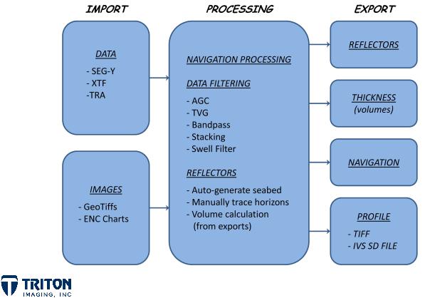
Following along the instructions in this booklet will introduce you to most of the options available within SB-Interpreter. A brief overview of the training program is presented below:
Data Import
•Sub-bottom data (SEG-Y, XTF, TRA files)
•GeoTiffs (Chart, Aerial/Sat. Imagery, Bathy/Sidescan)
Processing and Interpretation
•Navigation Smoothing and Line Intersection Check
•Data Filtering (AGC, TVG, Bandpass, etc.)
•Auto-generate Seabed, Draw Reflectors/Horizons
•Volume Calculations
Export to Other Programs
•Saving Profile and Processed Navigation to SEG-Y
•Export Individual or Folded Profile to IVS 3D object
Page 1
Chapter 2 – Map Window
MAP WINDOW REVIEW
SB-Interpreter has two primary interfaces. These are a GIS-based map window of the project data and a profile window to display vertical sections. In this chapter we will review the map window and most of the options available. The remaining options, profile folding, exporting and printing, will be reviewed later in the training guide.
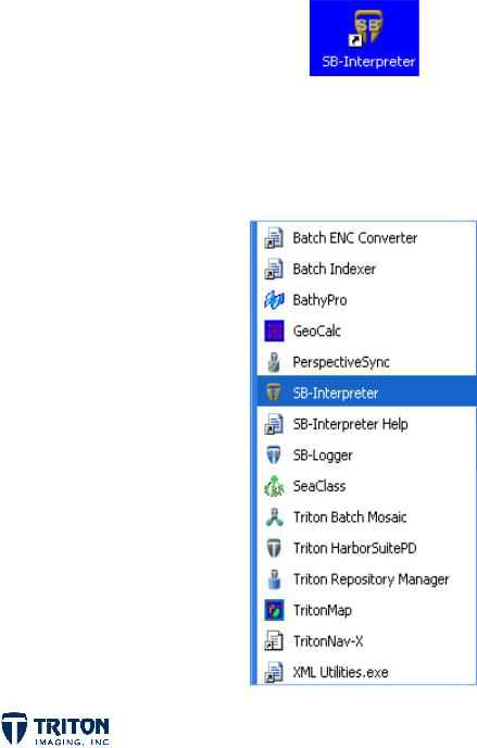
STEP 1: Open Program
Launch from Desktop Icon
OR
Launch from Start Menu
Page 2

MAP WINDOW REVIEW
Upon launching SB-Interpreter, the map window will open as shown above. Important things to note are:
•Map View – This is a GIS based view of the project data. Survey tracklines are displayed using the embedded navigation in the seismic files. Geo-referenced imagery can be used as a backdrop for spatial referencing.
•File Tree – This is where the imported files will be listed. For background images, files higher in the tree list will display in the map view over images lower in the tree list.
•Cursor Tab – Shows the position of the cursor in the map view. If the data is projected, the Northing and Easting will be displayed in addition to the Latitude and Longitude.
•Measure Tab – Shows the results of measurements made in the map view. In addition to the distance, the component distances in the X and Y directions are also displayed.
•Toolbar – Common tools used for importing data and navigating the map view are available in the toolbar. Many of these tools are located in the menu options as well.
Page 3

IMPORTING SUB-BOTTOM DATA
There are currently 3 file types compatible with SB-Interpreter:
a.SEG-Y (*.seg, *.sgy, *.segy)
b.Triton XTF (*.xtf)
c.Delph SEG-Y (*.tra)
Sub-bottom files can be imported into the project from the ‘File’ menu, toolbar buttons, and by right-clicking in the ‘Seismic Files’ section of the file tree via two methods. These options are:
a.Import File – can select a single file or multiple files in a folder
b.Import Folder – brings in all files in a selected folder
By default SB-Interpreter assumes that the navigation data are in Lat/Lon related to the WGS84 datum. If so, SB-Interpreter will read the navigation, automatically selecting the correct UTM Grid Zone. If the navigation is projected, a projection dialog box will pop up.
It is possible to set the projection prior to importing data in the ‘Projections’ tab in ‘Application Settings’ in the ‘View’ menu. This is important if the navigation coordinates in the data file are in Lat/Lon coordinates, but they are related to another datum than WGS84.
Page 4

IMPORTING SUB-BOTTOM DATA
For this training guide our demo data is in Lat/Lon so SB-Interpreter will automatically set the display projection.
STEP 2: Import Data Files
a.Select ‘Import Folder’ from the ‘File’ menu
b.Select the folder where the demo data was copied to on your hard drive …/DemoFiles/SB-I_DemoFiles/SEGY
Once complete, the map view now shows the location of the imported profile lines and the file tree contains line names and reference numbers for each line (P0 to P5).
Another thing that occurs upon import is the creation of cache files in the SEGY folder. The creation of these cache files is an integral part of the processing and only occurs once, the next time you access these files they will load more quickly.
Page 5

IMPORTING BACKGROUND IMAGES
•There are 3 background file types compatible with SB-Interpreter:
a.GeoTiff (*.tif, *.tiff)
with embedded spatial data or *.tfw file
b.Geo-referenced JPEG (*.jpg, *.jpeg)
must have *.jgw file
c.ENC Chart (*.enc)
must have ENC license to activate this option
•SB-Interpreter currently only supports geo-referenced background images with coordinates in meters.
•In the current release of SB-Interpreter there is a limit to the size of any single image, the maximum number of pixels is around 12,000 x 12,000. If this size is exceeded an ‘Out of Memory’ error will result.
Page 6
IMPORTING BACKGROUND IMAGES
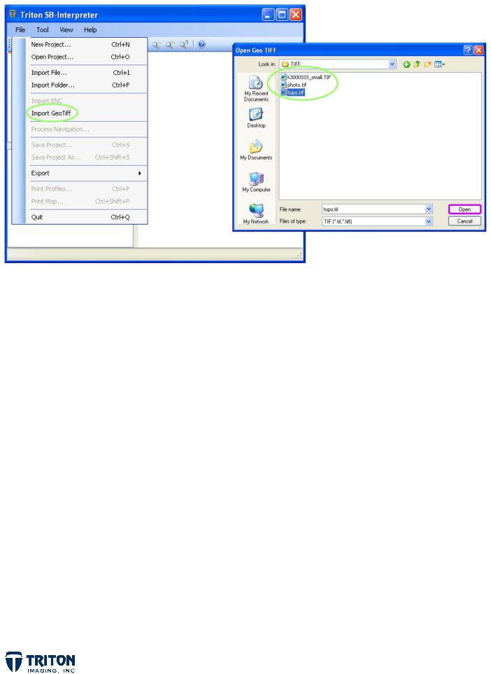
Background imagery can be imported into the project by selecting the ‘Import GeoTiff’ option from the ‘File’ menu, or by right-clicking in the ‘GeoTiff Cells’ section of the file tree and selecting ‘Add Layer’.
STEP 3A: Import Images:
a.Select ‘Import GeoTiff’ from the ‘File’ menu
b.Select the folder where the demo data was copied to on your hard drive
…/DemoFiles/SB-I_DemoFiles/TIFF
c. Select the file ‘Topo.tif’
For background imagery, the import projection must be manually set. This can be accomplished prior to importing via the ‘Projections’ tab in ‘Application Settings’ (as mentioned previously) or at the time of import.
Page 7
IMPORTING BACKGROUND IMAGES
The projection only needs to be set once. The same projection will then be used for all subsequent background imports.
STEP 3A: Import Images (cont.)
d.Select ‘Universal Transverse Mercator’
e.Select ‘Zone 18 North’
f.Select ‘WGS Datum (1984)’
g.Repeat import process for remaining image files (photo.tif & k3000SSS_small.tif)
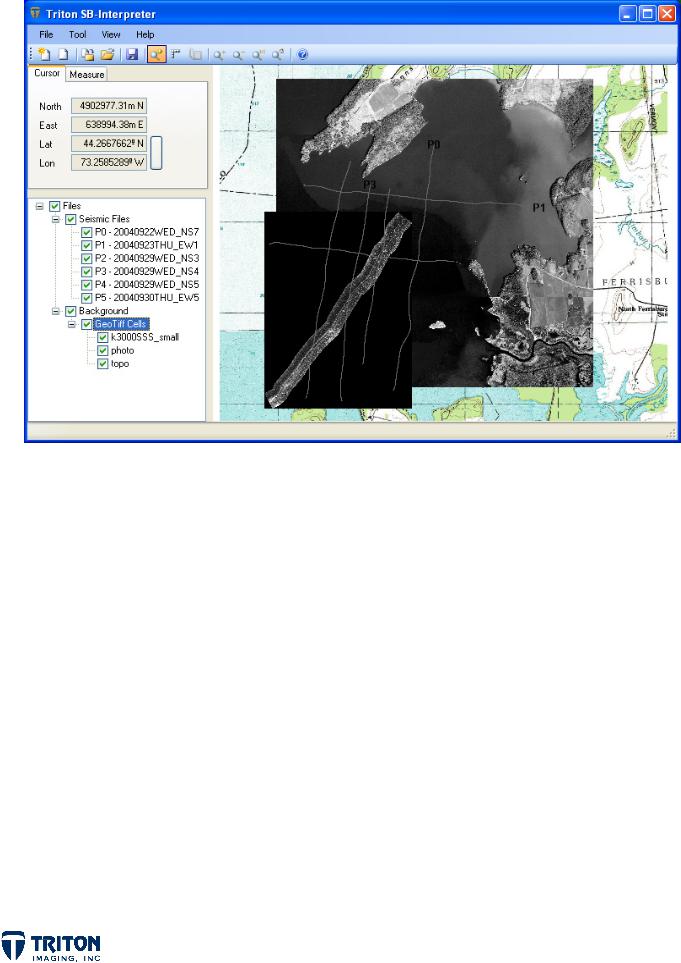
This will bring in the three background images layered on top of one another as shown on the following page.
Page 8
BACKGROUND IMAGE ADJUSTMENTS
As mentioned previously, the file tree order controls the order of files displayed in the map view. The tiffs located higher in the file tree structure are shown on top of those lower in the file tree. In this example the sidescan tiff is on top of the aerial photo, which is displayed over the background topo.
There are a few options in SB-Interpreter that can make these images more useful for spatial referencing. By right-clicking on the individual tiffs, the file tree order and transparency settings can be changed.
One of the more obvious changes needed is to remove the ‘no data’ region of the sidescan tiff. If we decide we want the chart (topo) to overlay the aerial photo, we can either move the photo down in the list or move the chart up the list and also change its transparency so we can still view the aerial photo now located beneath it.
Page 9
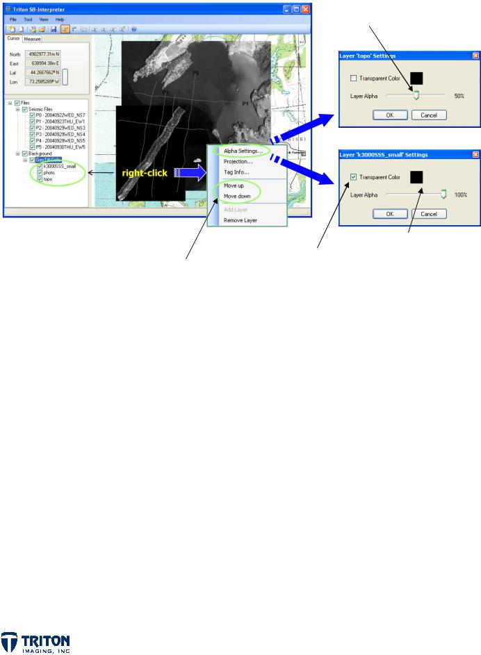
Use the sliding bar to control the amount of transparency
|
|
Image color chosen to be |
|
|
Check box for making |
transparent, to change |
|
To change the order, |
click on color and select |
||
selected color |
|||
right click on the GeoTiff |
transparent |
alternate color |
|
and select ‘Move up’ or |
|
|
|
‘Move down’ |
|
|
BACKGROUND IMAGE ADJUSTMENTS
Image adjustments are made by right-clicking on the individual tiffs. Options for adjusting the background images include changing the view order and adjusting transparency in ‘Alpha Settings’.
STEP 3B: Image Adjustments
a.Right-click on ‘photo’ in the file tree and select ‘Move down’
b.Right-click on ‘topo’ in the file tree and select ‘Alpha Settings’
Change the ‘Layer Alpha’ value to 50% using the slider bar
c.Right-click on ‘k3000SSS_small’ in the file tree and select ‘Alpha Settings’
Check ‘Transparent Color’ box for making selected color transparent
Select ‘Black’ as image color to be transparent
These quick adjustments allow the user to see the topo chart draped over the aerial photo with the sidescan image shown crossing the sub-bottom survey lines.
Page 10

BACKGROUND IMAGE ADJUSTMENTS
With the aerial photo showing through the chart, the default color for the sub-bottom profile navigation lines is too dark. Color options for survey navigation are located in the ‘Application Settings’.
STEP 3B: Image Adjustments (cont.)
d.Select the ‘Colors’ tab in ‘Application Settings’ in the ‘View’ menu
e.Click on the current color for ‘Navigation’
f.Select ‘Yellow’ as the new color
Adjusting the background imagery and default color settings in the map view assists with interpretation by allowing cross-referencing between data types (multibeam, sidescan, and sub-bottom) and regional features shown in topo maps, navigation charts and aerial photographs.
Page 11

PROCESS NAVIGATION
An important step to take once the sub-bottom data is imported is to process the navigation in the data files. This process will smooth navigation and place markers in each sub-bottom line at locations where lines intersect.
Navigation processing can be launched from the ‘File’ menu or by right-clicking on individual data files to process just that lines navigation or on the root ‘Seismic Files’ folder to process the navigation for all files.
STEP 4: Navigation Processing
a.Select ‘Process Navigation’ in the ‘File’ menu
b.Select ‘Filter Setup’
This will open a new window called ‘Boxcar Settings’ with options for filtering the raw navigation data. It is important to note that navigation smoothing does not affect the original data. The results are stored in cache files which are placed in the same folder as the data files but have a *.sgc file extension for SEG-Y files and *.xtc for XTF files.
Page 12
PROCESS NAVIGATION
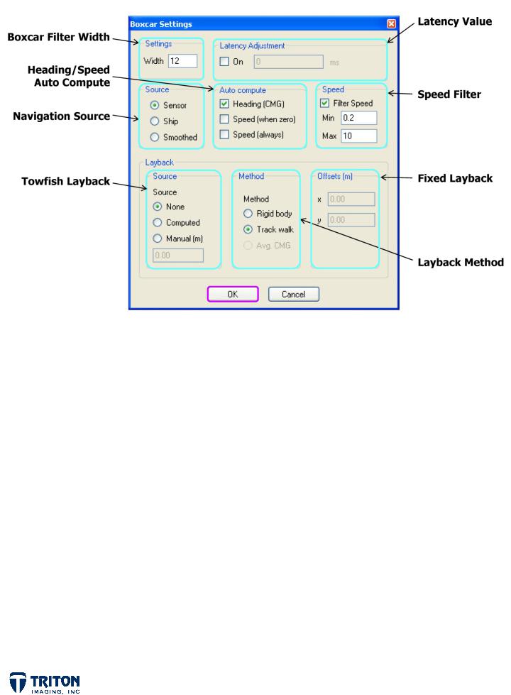
Boxcar Settings is a collection of common navigation processing steps for removing errors in navigation data. A brief description of the processing parameters and their options is presented below.
Boxcar Filter Width
•A larger number smoothes over a longer time period
Latency Value
•If known, latency values for the acquisition system can be entered here
Towfish Layback Source
•Use ‘None’ if hull mounted or if navigation is from the sensor
•‘Computed’ calculates layback from x-y values entered in ‘Offsets’ field or from values stored in XTF file
•‘Manual’ is for a fixed cable out value
Navigation Source
•‘Smoothed’ is for the previously smoothed navigation stored in cache file
Auto Compute
•Use this if heading or speed is not available in original file
Speed Filter
•Removes large jumps in navigation by removing values outside known speed range
Layback Method
•‘Rigid body’ will use the heading computed or stored in the cache file
•Track walk - project the entered layback value back along the vessel track to compute the position
Offsets (Fixed Layback)
•Location to manually enter static layback value or fixed offsets
Page 13
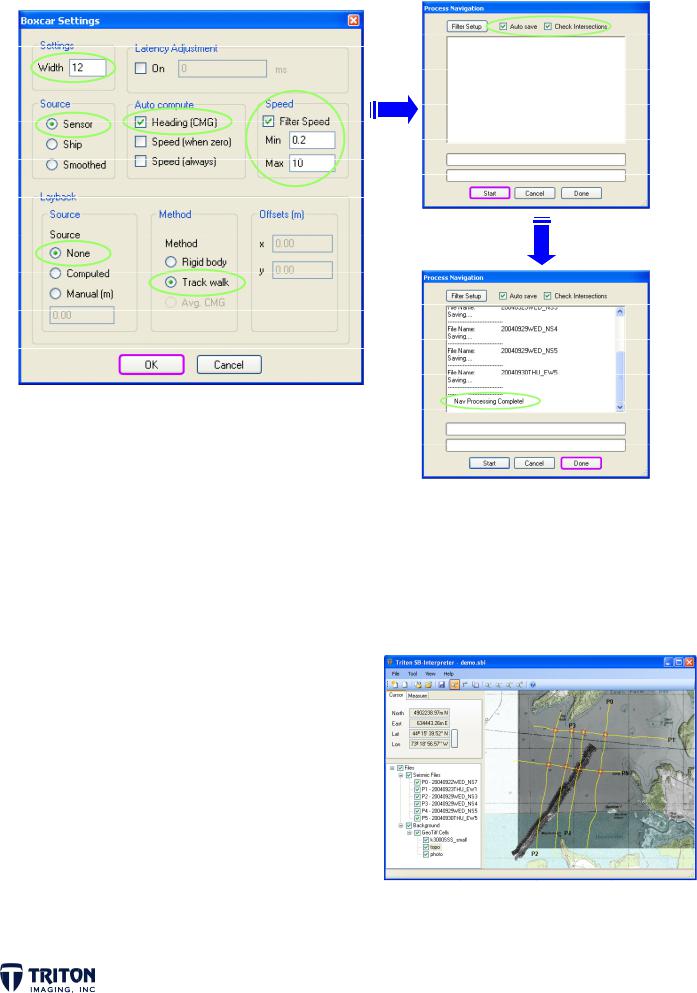
PROCESS NAVIGATION
STEP 4: Navigation Processing (cont.)
c. Select the options shown above in the ‘Boxcar Settings’ window a nd select ‘OK’ ( closes ‘Box car Setting s’ and retu rns you to ‘Process N avigation’)
d.In the ‘Process Navigation’ window, verify the ‘Auto s ave’ and ‘C heck Inter sections’ boxes are checked and then click ‘Start’
e.W hen finished, scroll down in the
‘P rocess Na vigation’ window to verify navigation processing is complete, then click ‘Done’ to close the window
Navigation lines hav e been smoothed per options chosen in the filter setup. Pla ces where li nes cross are identified as intersections and s hown in the map view as r ed circles. The intersections are important when viewing seismic sections and correlating reflecto rs/horizons across lines and for profile folding.
Page 1 5
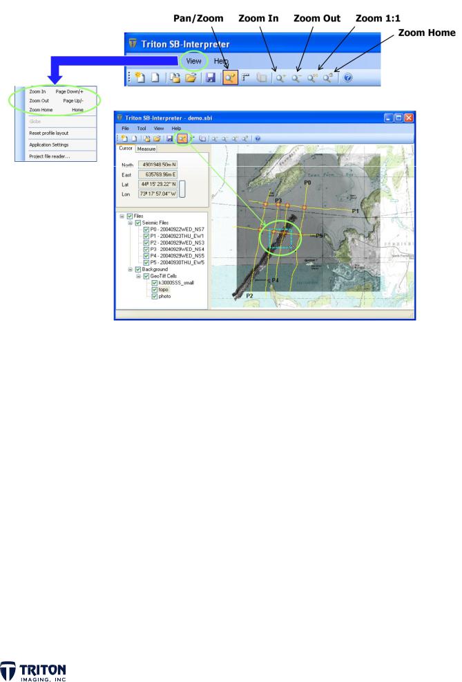
MAP VI EW PAN/Z OOM OPTIONS
Now that we have all of our files of intere st in the map view, th ere are a se veral options for moving around the map. As sh own earlier, there are 5 zoom but ton options with some of these also available under the ‘View’ menu.
Pan/Zoom |
pan across scr een (left click) and drag a specifie d zoom ext ent (right-click) |
Zoom In |
zoom in one level |
Zoom Ou t |
zoom out one l evel |
Zoom 1:1 |
zoom to 1 pixel by 1 pixel |
Zoom Ho me |
zoom to full extent of project data and background imager y |
In addition to zooming options, we may want to meas ure line spa cing or the swath coverage of an inser ted sidescan tiff.
STEP 5: Map Vie w Measure ments
a. Select the ‘Pan/Zoom’ toolbar button and z oom to are a shown on map above
Page 1 6
 Loading...