Rockwell Automation 1771-QB User Manual

Linear Positioning Module

Cat. No. 1771-QB

User Manual

Important User Information

Because of the variety of uses for the products described in this publication, those responsible for the application and use of this control equipment must satisfy themselves that all necessary steps have been taken to assure that each application and use meets all performance and safety requirements, including any applicable laws, regulations, codes and standards.

The illustrations, charts, sample programs and layout examples shown in this guide are intended solely for purposes of example. Since there are many variables and requirements associated with any particular installation, the Allen-Bradley Company, Inc. does not assume responsibility or liability (to include intellectual property liability) for actual use based upon the examples shown in this publication.

Allen-Bradley Publication SGI-1.1, “Safety Guidelines for the Application, Installation and Maintenance of Solid State Control” (available from your local Allen-Bradley office) describes some important differences between solid-state equipment and electromechanical devices which should be taken into consideration when applying products such as those described in this publication.

Reproduction of the contents of this copyrighted manual, in whole or in part, without written permission of the Allen-Bradley Company Inc. is prohibited.

Throughout this manual we use notes to make you aware of safety considerations:

ATTENTION: Identifies information about practices or circumstances that can lead to personal injury or death, property damage or economic loss.

Attentions help you:

identify a hazard avoid the hazard recognize the consequences

Important: Identifies information that is especially important for successful application and understanding of the product.

PLC is a registered trademark of Allen-Bradley Company, Inc.

Word Assignment 62 Module Configuration Word (word 1) 62 Status Word 1 (words 2 and 6) 63 Status Word 2 (words 3 and 7) 67 Position/Error/Diagnostic Words 69 Active Motion Segment/Setpoint (words 10 and 11) 613 Measured Velocity (words 20 and 21) 614 Desired Velocity (words 22 and 23) 614 Desired Acceleration (words 24 and 25) 615 Desired Deceleration (words 26 and 27) 615 Percent Analog Output (words 28 and 29) 616 Maximum Velocity (words 30, 31 and 32, 33) 617

. . . . . . . . . . . . . . . . . . . . . . . . . . . . . . . . . . . . . . .

. . . . . . . . . . . . . . . . . . . . . . . . . . . . . . . . . .

. . . . . . . . . . . . . . . . . . . .

. . . . . . . . . . . . . . . . . . . . . . . .

. . . . . . . . . . . . . . . . . . . . . . .

. . . . . . . . . .

. . . . . . . . . . . . . . . . . . .

. . . . . . . . . . . . . . . . . . . . .

. . . . . . . . . . . . . . . . . .

. . . . . . . . . . . . . . . .

. . . . . . . . . . . . . .

Formatting Module Data (WRITES) 71. . . . . . . . . . . . . . . . . . .

Data Blocks Used in Write Operations 71. . . . . . . . . . . . . . . . . . . . .

Parameter Block (Required) 71 Setpoint Block (Optional) 71 Command Block (Required) 71

Parameter Block 71

Parameter Control Word (word 1) 73 Analog Range (words 2 and 31) 75 Analog Calibration Constants (words 3, 4 and 32, 33) 76 Transducer Calibration Constant (words 5, 6 and 34, 35) 77 ZeroPosition Software Travel Limits (words 9, 10 and 38, 39) 79 ZeroPosition and Software T InPosition Band (words 11 and 40) 713 PID Band (words 12 and 41) 714 Deadband (words 13 and 42) 715 Excess Following Error (words 14 and 43) 716 Maximum PID Error (words 15 and 44) 716 Integral Term Limit (words 16 and 45) 717 Proportional Gain (words 17 and 46) 718 Gain Break Speed (words 18 and 47) 719

. . . . . . . . . . . . . . . . . . . . . . . . . . . . . . . . . . . .

Of

fset (words 7, 8 and 36, 37) 78. . . . . . . . . . . . . . .

. . . . . . . . . . . . . . . . . . . . . . . . . .

. . . . . . . . . . . . . . . . . . . . . . . . . . . .

. . . . . . . . . . . . . . . . . . . . . . . . . .

. . . . . . . . . . . . . . . . . . . . . .

. . . . . . . . . . . . . . . . . . . . . . .

. . . . . . . .

. . . . . .

. . . . . . . . . . . .

ravel Limit Examples

. . . . . . . . . . . . . . . . . . . . .

. . . . . . . . . . . . . . . . . . . . . . . . . .

. . . . . . . . . . . . . . . . . . . . . . . . .

. . . . . . . . . . . . . . . .

. . . . . . . . . . . . . . . . . .

. . . . . . . . . . . . . . . . . . .

. . . . . . . . . . . . . . . . . . . .

. . . . . . . . . . . . . . . . . . .

710. . . . . . . . . .

Table of Contentsiv

Gain Factor (words 19 and 48) 720. . . . . . . . . . . . . . . . . . . . . . . .

Integral Gain (words 20 and 49) 721 Derivative Gain (words 21 and 50) 722 Feedforward Gain (words 22 and 51) 722 Global Velocity (words 23 and 52) 723 Global Acceleration/Deceleration (words 24, 25 and 53, 54) 724 Velocity Smoothing (Jerk) Constant (words 26 and 55) 724 Jog Rate (Low and High) (words 27, 28 and 56, 57) 726 Reserved (words 29, 30 and 58, 59) 727

Setpoint Block 727

Setpoint Block Control Word (word 1) 729 Incremental/Absolute Word (word 2) 729 Setpoint Local Velocity 731 Local Acceleration/Deceleration 732

Command Block 732

Axis Control Word 1 (words 1 and 8) 733 Axis Control Word 2 (words 2 and 9) 738 Setpoint 13 Words (words 3 to 7 and 10 to 14) 739

. . . . . . . . . . . . . . . . . . . . . . . . . . . . . . . . . . . . . .

Position

. . . . . . . . . . . . . . . . . . . . . . . . . . . . . . . . . . . .

. . . . . . . . . . . . . . . . . . . . . . .

. . . . . . . . . . . . . . . . . . . . . .

. . . . . . . . . . . . . . . . . . . .

. . . . . . . . . . . . . . . . . . . . . .

. . . .

. . . . . . .

. . . . . . . . .

. . . . . . . . . . . . . . . . . . . .

730. . . . . . . . . . . . . . . . . . . . . . . . . . . . . . . . . .

. . . . . . . . . . . . . . . . . . . . . . .

. . . . . . . . . . . . . . . . . . . .

. . . . . . . . . . . . .

Initializing and Tuning the Axes 81. . . . . . . . . . . . . . . . . . . . .

Before You Begin 81. . . . . . . . . . . . . . . . . . . . . . . . . . . . . . . . . . . .

Adjusting the Servo V Initializing the Parameter Block 82 Verifying Verifying Transducer Calibration Constants 87 Axis Tuning 810

Analog Output Polarity

. . . . . . . . . . . . . . . . . . . . . . . . . . . . . . . . . . . . . . . .

Analog Calibration Constants 810 Feedforward PID Loop Gains 812 Update the Application Program 813

alve Nulls

. . . . . . . . . . . . . . . . . . . . . . . . . .

. . . . . . . . . . . . . . . . .

. . . . . . . . . . . . . . . . . . . . . . . . .

Gain

. . . . . . . . . . . . . . . . . . . . . . . . . . . . . . . . . . .

. . . . . . . . . . . . . . . . . . . . . . .

82. . . . . . . . . . . . . . . . . . . . . . . . . .

87. . . . . . . . . . . . . . . . . . . . . . . . .

811. . . . . . . . . . . . . . . . . . . . . . . . . . . . . . . . .

Advanced Features 91. . . . . . . . . . . . . . . . . . . . . . . . . . . . . .

Motion Block 91. . . . . . . . . . . . . . . . . . . . . . . . . . . . . . . . . . . . . . .

Motion Block Control Word 94

Programmable

Programmable Default

Motion Segments 98

Motion Segment Control Words 98 Desired

and Local Deceleration Words 911

Trigger V

The Command Block and the Motion Block 911 The Status Block and the Motion Block 911

Input and Output

I/O Control W

I/O Configuration

. . . . . . . . . . . . . . . . . . . . . . . . . . . . . . . . . . . .

Position, Local V

elocity/Position W

. . . . . . . . . . . . . . . . . . . . . . . . . . .

95. . . . . . . . . . . . . . . . . . . . . . . . .

ord 95. . . . . . . . . . . . . . . . . . . . . . .

98. . . . . . . . . . . . . . . . . . . . . . . . . . . . .

. . . . . . . . . . . . . . . . . . . . . . . .

elocity, Local Acceleration

. . . . . . . . . . . . . . . . . . . . . .

ords 911. . . . . . . . . . . . . . . . . . . . . . . .

. . . . . . . . . . . . . . . . . .

. . . . . . . . . . . . . . . . . . . .

Table of Contents v

Using

the Motion Block

Sample Application Programs 101. . . . . . . . . . . . . . . . . . . . . .

912. . . . . . . . . . . . . . . . . . . . . . . . . . . . . . . .

Programming Block Transfer Sequencing 102 PLC5 Block Transfer Instructions 103 Application Program #1 103

Planning the Data Blocks for Application Program #1 105 Program Rungs for Application Program #1 108

Application Program #2 1011

Planning the Data Blocks for Application Program #2 1012 Program Rungs for Application Program #2 1016

Objectives

101. . . . . . . . . . . . . . . . . . . . . . . . . . . . . . .

. . . . . . . . . . . . . . . . . . . . . . . . . . . . .

. . . . . . . . . . . . . . . . . . . . . . . .

. . . . . . . . . . . . . . . . . . . . . . . . . . . . . . .

. . . . . . . . .

. . . . . . . . . . . . . . .

. . . . . . . . . . . . . . . . . . . . . . . . . . . . . . .

. . . . . . . . .

. . . . . . . . . . . . . . .

Troubleshooting 111. . . . . . . . . . . . . . . . . . . . . . . . . . . . . . . .

Fault Indicators 111. . . . . . . . . . . . . . . . . . . . . . . . . . . . . . . . . . . . .

Module Loop Active Indicators 112

Indicator Troubleshooting Guide 112 Troubleshooting Feedback Faults 113 Troubleshooting Flowchart 114

Flowchart Notes 117

Fault Indicator

. . . . . . . . . . . . . . . . . . . . . . . . . . . . . . . . . . .

112. . . . . . . . . . . . . . . . . . . . . . . . . . . . . .

. . . . . . . . . . . . . . . . . . . . . . . . . . . . . .

. . . . . . . . . . . . . . . . . . . . . . .

. . . . . . . . . . . . . . . . . . . . . . . .

. . . . . . . . . . . . . . . . . . . . . . . . . . . . .

Glossary of Terms & Abbreviations A1. . . . . . . . . . . . . . . . . .

Status Block B1. . . . . . . . . . . . . . . . . . . . . . . . . . . . . . . . . . .

Parameter Block C1. . . . . . . . . . . . . . . . . . . . . . . . . . . . . . . .

Setpoint Block D1. . . . . . . . . . . . . . . . . . . . . . . . . . . . . . . . . .

Command Block E1. . . . . . . . . . . . . . . . . . . . . . . . . . . . . . . .

Motion Block F1. . . . . . . . . . . . . . . . . . . . . . . . . . . . . . . . . . .

Hexadecimal Data Table Forms G1. . . . . . . . . . . . . . . . . . . . .

Table of Contentsvi

Data Formats H1. . . . . . . . . . . . . . . . . . . . . . . . . . . . . . . . . . .

BCD H1. . . . . . . . . . . . . . . . . . . . . . . . . . . . . . . . . . . . . . . . . . . . .

2's Complement Binary H1

Bit Inversion Method H2 Subtraction Method H2

Decimal

Implied Position Format H3 Double Word Position Format H4

. . . . . . . . . . . . . . . . . . . . . . . . . . . . . . . .

H2. . . . . . . . . . . . . . . . . . . . . . . . . . . . . . . . . . . . .

. . . . . . . . . . . . . . . . . . . . . . . . . . . . . . . . . . . . .

. . . . . . . . . . . . . . . . . . . . . . . . . . .

Product Specifications I1. . . . . . . . . . . . . . . . . . . . . . . . . . .

Preface

This manual explains how to install and configure the Linear Positioning Module. It includes sample application programs to illustrate how to program a PLC to work with the Linear Positioning Module.

Organization of the Manual

This manual contains eleven chapters and nine appendices that address the following topics:

Chapter Title Describes:

1 Introducing the Linear Positioning

Module

2 Positioning Concepts concepts and principles of closedloop servo

3 Positioning with the Linear

Positioning Module

4 Hardware Description module hardware, module interfaces, and other

5 Installing the Linear Positioning

Module

6 Interpreting ModuletoPLC Data

(READS)

7 Formatting Module Data

(WRITES)

the functions and features of the Linear Positioning Module

positioning

using the Linear Positioning Module in a positioning system

hardware items you need for a positioning system

configuring the module's analog outputs and installing the module in your system

monitoring module operation from a logic controller by reading and interpreting data that the module transfers to the logic controller's data tables

formatting parameter, move description, and control data for block transfers to the Linear Positioning Module

8 Initializing and Tuning the Axes bringing the module online

9 Advanced Features using the motion block to perform blended moves;

using programmable input and output operations

10 Sample Application Programs two application programs, one using basic concepts

and the other using advanced features, to control and monitor the module

11 Troubleshooting using the module's indicators and the status block

to diagnose and remedy module faults and errors

Appendix A Glossary common terms and abbreviations

Appendix B Status Block status block word assignments

Appendix C Parameter Block parameter block word assignments

Appendix D Setpoint Block setpoint block word assignments

P1

Preface

Chapter Describes:Title

Appendix E Command Block command block word assignments

Appendix F Motion Block motion block word assignments

Appendix G Hexadecimal Data Table Form hexadecimal data worksheets

Appendix H Data Formats valid data formats

Audience

Related Publications

Related Software

Appendix I

Product Specifications

1771QB product specifications

Read this manual if you intend to install or use the Linear Positioning Module (Cat. No. 1771-QB).

To use the module, you must be able to program and operate an Allen-Bradley PLC. In particular you must be able to program block transfer instructions.

In this manual, we assume that you know how to do this. If you don’t, refer to the User Manual for the PLC you’ll be programming.

Consult the Allen-Bradley Industrial Computer Division Publication Index (SD 499) if you would like more information about your modules or PLCs. This index lists all available publications for Allen-Bradley programmable controller products.

The Hydraulics Configuration and Operation Option (Cat. No. 6190-HCO) operates within the ControlView Core (Cat. No. 6190-CVC) environment to provide full configuration and realtime monitoring for the Linear Positioning Module. Both software packages are available from:

P2

Allen-Bradley Company, Inc. 1201 South Second Street Milwaukee, WI 53204 (414) 382-2000

Servo Analyzer is a software package that aids in tuning the axes by letting you display an axis profile as you tune it. The resulting graphics may be plotted, printed or saved to a file. The software is available from:

Computer Software Design P.O. Box 962 Roseburg, OR 97470 (503) 673-8583

Preface

Frequently Used Terms

Appendix A contains a complete glossary of terms and abbreviations used in this manual.

To make this manual easier for you to read and understand, product names are avoided where possible. The Linear Positioning Module is also referred to as the “module”.

P3

Chapter

1

Introducing the Linear Positioning Module

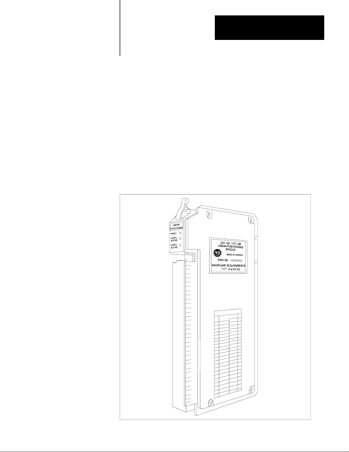
What is the Linear Positioning Module?

The Linear Positioning Module (Cat. No. 1771-QB) is a dual-loop position controller occupying a single slot in the Allen-Bradley 1771 Universal I/O chassis. It can control servo or proportional hydraulic valves, or some electric servos. Position is measured with a linear displacement transducer. You use the module to control and monitor the linear position of a tool or workpiece along one or two axes.

Figure 1.1

Positioning Module

Linear

50110

11

Chapter 1

Introducing the Linear Positioning Module

Product Compatibility

PLCs

You can use the module with any Allen-Bradley PLC that uses block transfer programming in local 1771 I/O systems including:

PLC-2 family

PLC-3 family

PLC-5 family

- PLC-5/10 (Cat. No. 1785-LT4)

- PLC-5/11 (Cat. No. 1785-LT11)

- PLC-5/12 (Cat. No. 1785-LT3)

- PLC-5/15 (Cat. No. 1785-LT)

- PLC-5/20 (Cat. No. 1785-L20)

- PLC-5/25 (Cat. No. 1785-LT2)

- PLC-5/30 (Cat. No. 1785-L30)

- PLC-5/40 (Cat. No. 1785-L40)

- PLC-5/60 (Cat. No. 1785-L60)

Transducers

The Linear Positioning (QB) Module is compatible with linear displacement transducers manufactured by:

MTS Systems Corporation Sensors Divisions Box 13218, Research Triangle Park North Carolina 27709 (919) 677–0100

Balluff Inc. P.O. Box 937 8125 Holton Drive Florence, KY 41042 (606) 727–2200

12

Chapter 1

Introducing the Linear Positioning Module

Santest Co. Ltd. c/o Ellis Power Systems 123 Drisler Avenue White Plains, NY 10607 (914) 592-5577

Lucas Schaevitz Inc. 7905 N. Route 130 Pennsauken, NJ 08110-1489 (609) 662-8000

All four manufacturers provide versions of the transducer that connect directly to the module’s wiring arm, without an external digital interface box. The module may also be compatible with other linear displacement transducers.

Servo and Proportional Valves

The module provides current ranges of up to +100 mA for direct interface to most servo valves, most proportional valves, and a + compatibility with other devices, such as electric servo interfaces. The module is compatible with valves supplied by the following manufacturers:

Moog, East Aurora NY servo/proportional

Parker Hannifin Corporation, Elyria OH servo/proportional

Robert Bosch Corporation proportional

Rexroth Corporation, Lehigh Valley PA servo/proportional

ATOS proportional

Atchley, Canaga Park CA servo

Pegasus servo

Vickers Inc., Grand Blanc, MI servo/proportional

The module may also be compatible with other valves. Important: Some proportional valves with LVDT loop controllers may limit

the module’s output and thus prevent the module from providing optimal control.

10 volt option for

13

Chapter 1

Introducing the Linear Positioning Module

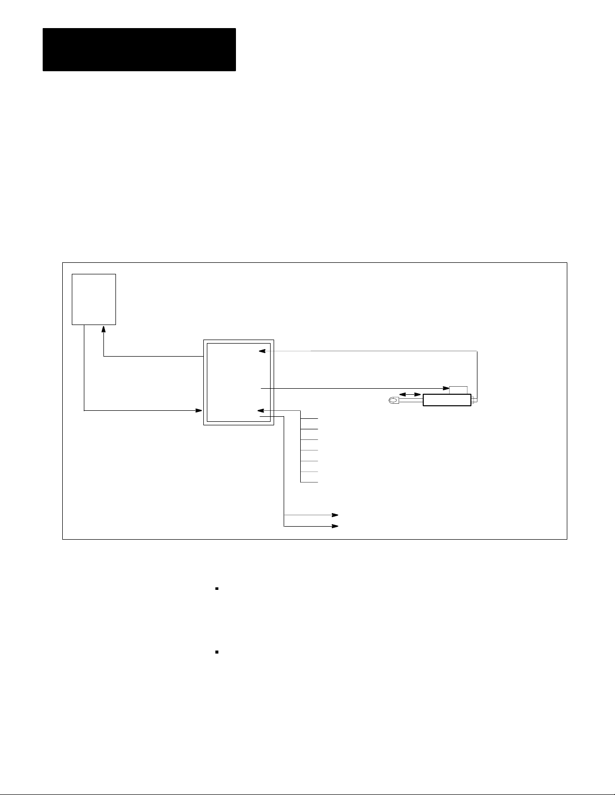
System Overview

PLC

Processor

D Status Block

D Parameter Block D Setpoint Block D Motion Block D Command Block

Figure 1.2 shows one of the module’s two control loops within a linear positioning system for closed-loop axis control. The module communicates with a programmable controller through the 1771 backplane.

The programmable logic controller sends commands and user-programmed data from the data table to the module as directed by a block-transfer write instruction.

Figure 1.2

Overview

System

Transducer

Interface

Linear

Positioning

Module

Discrete Inputs

D Jog Forward D Jog Reverse D Hardware Start D Auto/Manual D Hardware Stop D Input 1 D Input 2

Discrete Outputs

D

Analog Output

D Output 1 D Output 2

Servo Valve

Linear Displacement

Transducer

PistonType

Cylinder

NOTE: All inputs and outputs are duplicated for the second axis.

50033

14

Using PLC programming, you can:

send configuration and control parameters to the module via parameter,

setpoint, motion, and command blocks. With this data the module determines axis parameters, calculates velocity curves, and commands axis end-positions. (See Chapters 7 and 9.)

read status blocks to monitor axis position and status indicators in your

process control system. (See Chapter 6.)

The module’s analog outputs (one for each control loop) connect to servo or proportional valves via wiring arm terminals. The module controls speed and position by adjusting the voltage or current levels of the analog outputs 500 times each second.

Chapter 1

Introducing the Linear Positioning Module

The module also connects to linear displacement transducers (one for each of the two axes) via wiring arm terminals. The transducer senses the axis position and feeds it back to the module, thereby closing the control loop.

The module’s built-in processor samples the linear displacement transducer interfaces and determines positions along each of the two axes every two milliseconds. The module then updates the analog outputs based on a proprietary algorithm designed specifically to handle hydraulic actuators. This rapid update rate provides repeatable positioning and superior control of velocity without jerky movement.

Motion blocks provide for complex motions by allowing motion segments to be blended or chained together. These motion segments may also be synchronized using the hardware input triggers and outputs.

Cam emulation permits motion segments in one axis to start motion segments in another axis. Articulated motions and axis sequencing may be easily accomplished.

15

Chapter

2

Positioning Concepts

This chapter explains concepts and principles of axis positioning. If you are thoroughly familiar with the concepts of closed-loop servo positioning, you can go on to Chapter 3.

Axis Motion

Electric

Control

Hydraulic Fluid

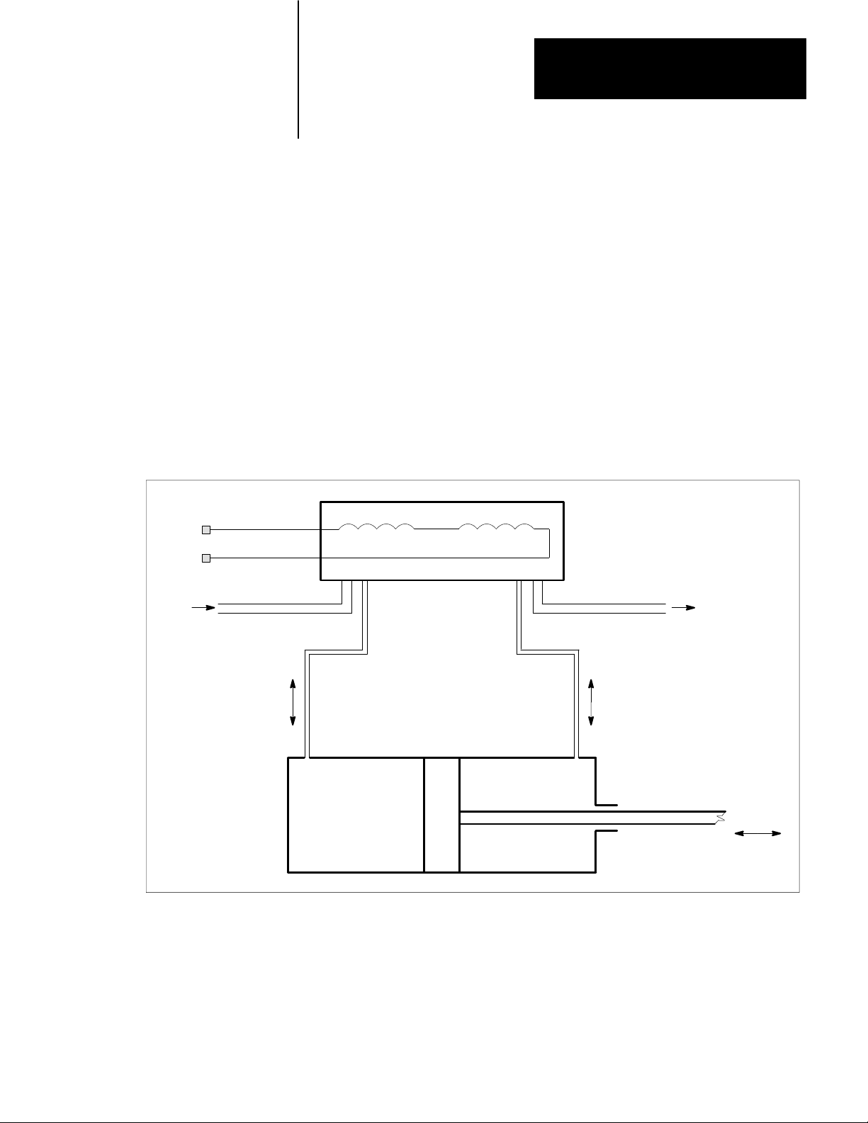
Figure 2.1 illustrates a typical method of converting the flow of fluid into a linear displacement.

Figure 2.1 PistonType

Hydraulic Cylinder

SERVO VALVE

Hydraulic Fluid

Axis Motion

Hydraulic fluid Hydraulic fluid

50032

The servo valve controls the flow of hydraulic fluid into or out of the hydraulic cylinder. Adding fluid to the left side of the cylinder extends the rod; adding fluid to the right side retracts it.

21

Chapter 2

Positioning Concepts

ClosedLoop Positioning

Closed-loop positioning is a precise means of moving an object from one position to another. In a typical application, a positioning device activates a servo valve controlling the movement of fluid in a hydraulic system. The movement of fluid translates into the linear motion of a hydraulic cylinder. A transducer monitors this motion and feeds it back to the positioning device. The positioning device, in turn, calculates a positioning correction and feeds it back to the servo valve.

Important: Throughout this manual we refer to servo valves, but you can also use the analog outputs to control proportional valves or an electric servo.

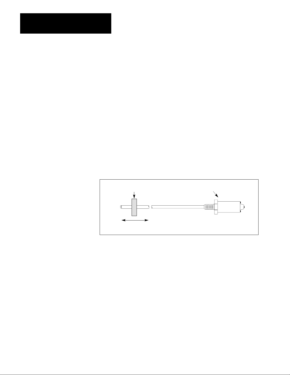
Linear Displacement Transducer

A linear displacement transducer (see Figure 2.2) is a device that senses the position of an external magnet to measure displacements.

Figure 2.2

Displacement T

Linear

Magnet

ransducer

Transducer Head

22

Magnet mounted to the piston of actuator

50034

The transducer sends a signal through the transducer wave guide where a permanent magnet generates the return pulse. You can use the time interval between the transducer’s signal and the return pulse to measure axis displacement.

Circulations

Some linear displacement transducers provide circulations or recirculation to improve resolution. (See Figure 2.3.) This technique stretches the pulse by a factor of two or more and results in finer resolution in the circuitry monitoring the pulse width.

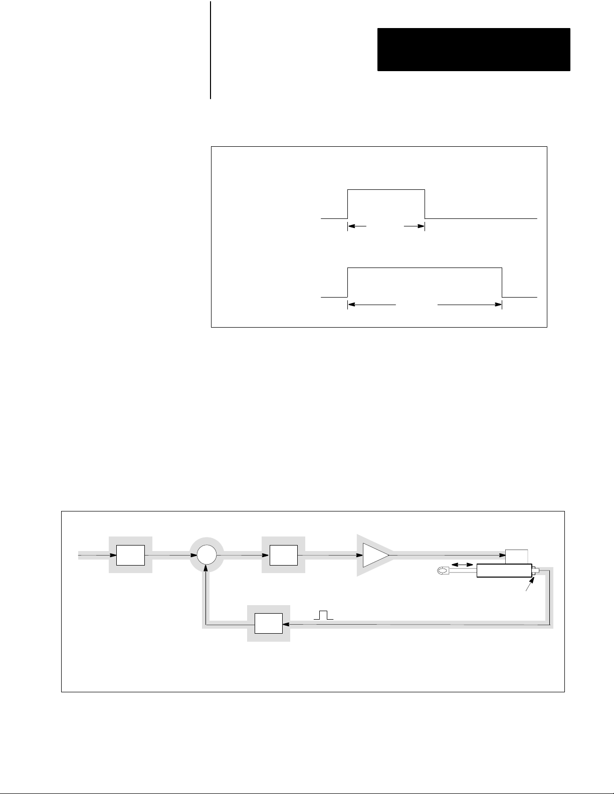
Figure 2.3 Circulations

Gate (received from transducer)

Chapter 2

Positioning Concepts

resolution = 0.002

Duration

(1 circulation)

resolution = 0.001

Duration

(2 circulations)

50035

Desired Velocity

dt

s

Integrator

Position Command

A Simple Positioning Loop

To move a specified distance along an axis, you can command the hydraulic device to move at a specific velocity for a specific length of time. However, this method can be imprecise. To control the position of the hydraulic device accurately you need a loop to monitor actual position. Figure 2.4 shows a simple positioning loop.

Figure 2.4 Positioning

Following Error

+

Actual

Position

Loop

dt

s

Kp

D/A

Velocity Command

Axis

Servo Valve

Linear Displacement Transducer

50036

23

Chapter 2

Positioning Concepts

In Figure 2.4:

desired velocity is the desired speed of axis motion from one position to

another

position command equals the integration of velocity over time actual position value (transducer feedback) is the actual position of the

axis as measured by the LDT

following error equals position command minus actual position velocity command is generated by amplifying the following error and

converting the result into an analog output

D/A (Digital to Analog convertor) generates the analog output controlling the

servo valve

KP (proportional gain) is the component that causes an output signal to

change as a direct ratio of the error signal variation

Proportional Gain

The following error is a function of the velocity command divided by the proportional gain (K following error by the proportional gain. Proportional gain can be expressed in ips/mil (where 1 mil = 0.001 inches) or mmps/mil (where 1 mil = 0.001 mm).

For example, with a velocity of 12 ips and a gain of 1 ips/mil, the following error is:

Following Error = Velocity/Gain

When you increase the gain, you decrease the following error and decrease the cycle time of the system. However, the capabilities of the system limit the gain. Too large a gain causes instability.

). To generate the velocity command, multiply the

P

= 12 ips/(1 ips/mil) = 12 mil

24

Chapter 2

Positioning Concepts

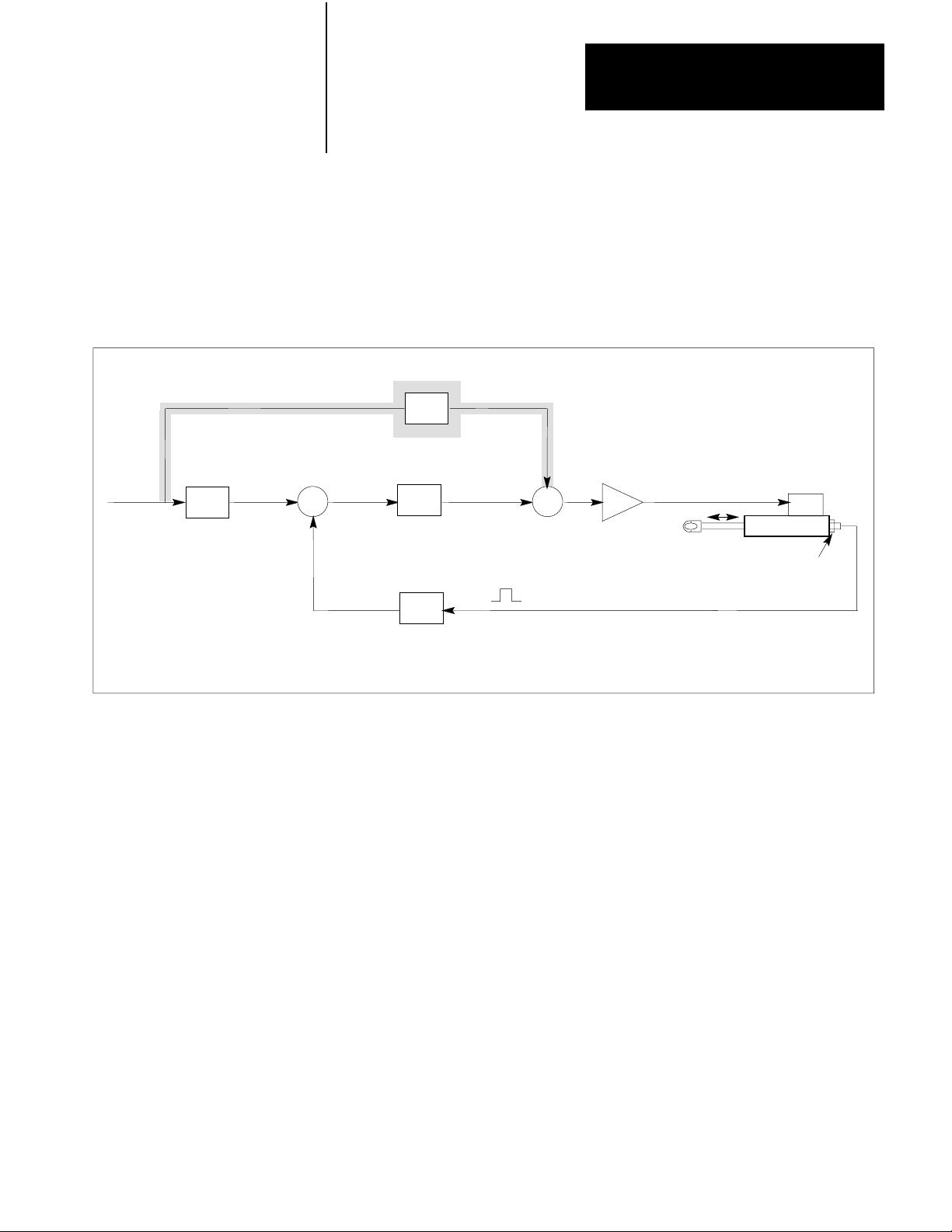
Feedforwarding

To decrease the following error without increasing the gain, you can add a feedforward component. (See Figure 2.5.)

Desired Velocity

dt

s

Integrator

Position Command

Figure 2.5

Loop with Feedforwarding

Feed Forward

+

Kp

s

K

F

dt

Velocity Command

D/A

Axis

+

-

Positioning

Following Error

Actual Position

Feedforwarding requires an additional summing point and an amplifier. Multiply the desired velocity by the feedforward gain K

to produce a

F

feedforward value. The feedforward value, added to a multiplication of the following error by the proportional gain (K

), generates the velocity command.

P

Servo Valve

Linear Displacement Transducer

50037

Without feedforwarding, axis motion does not begin until the following error is large enough to overcome friction and inertia. The feedforward component generates a velocity command to move the cylinder almost immediately. This immediate response keeps the actual position closer to the desired position and thereby reduces the following error.

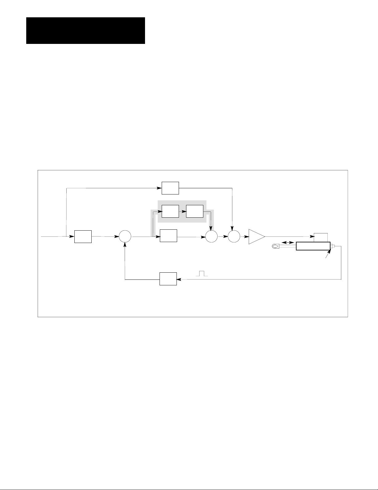
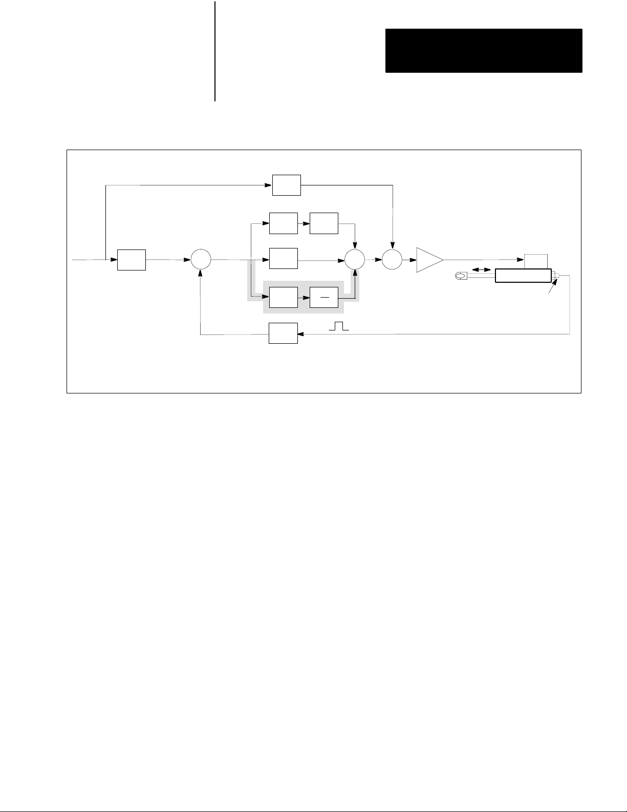
Integral Control (Reset Control)

You can increase the positioning accuracy of the control loop by adding an integral component. (See Figure 2.6.)

To achieve the integral component of the positioning loop, integrate the following error over time and amplify it to produce an integral value. Then add this integral value to the proportional component and the feedforward value to generate the velocity command.

25

Chapter 2

Positioning Concepts

Without integral control, the axis responds only to the size of the positioning error, not its duration. Integral control responds to both the size and duration of the positioning error. Thus, the integral term continues to adjust the velocity command until it achieves an exact correction.

Desired Velocity

dt

s

Integrator

Position Command

When you increase the integral gain (K

), you increase the rate at which the

I

positioning loop responds to a following error. However, the capabilities of the system limit gain K

Figure 2.6 Integral

Following Error

+

-

Actual Position

Control

s

K

Kp

dt

Too large a gain causes instability.

I.

Feed

F

I

Forward

Integrator

dt

s

+

Velocity Command

D/A

Axis

Servo Valve

Linear Displacement Transducer

26

50038

Derivative Control (Rate Control)

Proportional and integral gains can cause instability in a positioning loop. The cylinder can overshoot its programmed endpoints and oscillate or hunt around them. You can increase the stability of the positioning loop by adding a derivative component. (See Figure 2.7.)

Derivative control operates on the rate of change of positioning error. It helps to stabilize the system by opposing changes in positioning error. However, a derivative gain that is too large can cause instability. Derivative control is also very susceptible to electrical noise.

Chapter 2

Positioning Concepts

Desired Velocity

dt

s

Integrator

Position Command

Figure 2.7 Derivative

Following Error

+

-

Actual Position

Control

K

Kp

K

s

I

D

dt

F

Feed Forward

Integrator

dt

s

Derivative

d dt

D/A

Velocity Command

Servo Valve

Axis

Linear Displacement Transducer

50039

+

Deadband

Most systems have friction and play in their mechanical linkages. These characteristics can cause a cylinder to oscillate around a programmed endpoint–especially if you use an integral term. You can use a deadband to reduce these oscillations.

A deadband is an area surrounding the programmed endpoint where the error is ignored. Outside the deadband, error is reduced by one half the width of the deadband.

If you apply a deadband to an integral term, the integral output remains constant while the axis is within the deadband. This reduces oscillations around the endpoint. However, if the deadband is too large, it can also reduce the positioning accuracy of the system.

PID Band

Integral and derivative control can cause undesirable results when the axis moves from one position to another. The integral term can cause the axis to overshoot the programmed endpoint. The derivative term opposes changes in error, and thereby changes in position.

27

Chapter 2

Positioning Concepts

You can control the integral and derivative components by defining a PID (proportional, integral and derivative) band. The PID band is a region surrounding the programmed endpoint where the system enables integral or derivative terms. As a result, the integral and derivative components affect only the final positioning of the axis.

28

Chapter

3

Positioning with the Linear Positioning Module

This chapter explains how the Linear Positioning Module interacts with a programmable controller to control axis movement within a linear positioning system.

How the Module Fits in a Positioning System

1771-QB MODULE

Desired Velocity

Integrator

s

Position Command

dt

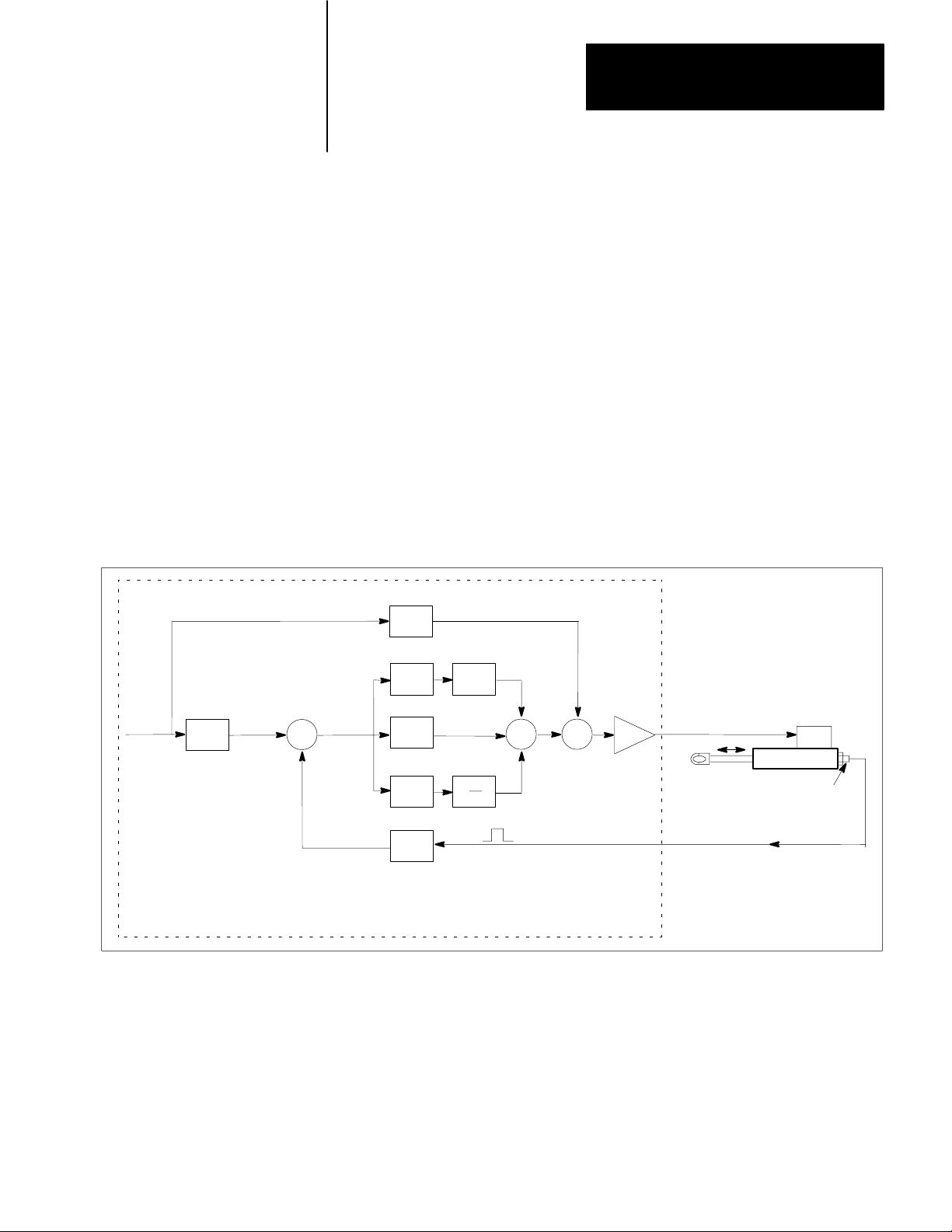
Figure 3.1 shows how the module functions in a typical positioning system. Note that the positioning loop closes in the module and functions independently of the programmable controller’s I/O scan rate. The fast loop update time of 2 ms is possible, because the module has a built-in microprocessor.

Figure 3.1

Module in a Positioning System

The

Feed

K

F

K

s

I

Kp

K

D

dt

Following Error

+

-

Actual Position

Forward

Integrator

dt

s

Derivative

d dt

+

D/A

Velocity Command

Axis

Servo Valve

Linear Displacement Transducer

50040

31

Chapter 3

Positioning with the Linear Positioning Module

How the Module Interacts with a PLC

The module is a dual-loop position controller, occupying a single slot in the Allen-Bradley 1771 universal I/O chassis. The module communicates with the PLC through the 1771 backplane. There are two kinds of transfers–read operations and write operations. By programming the PLC you can transfer parameter, setpoint, motion and command blocks to the module to control the two axes. You can also use the PLC to monitor the status of the module’s two loops through block read operations. For more details on block transfers, see Chapters 6 and 7.

Read Operations

Read operations enable the programmable logic controller to monitor the status of both axes through the status block. The status block includes detailed information on the two axes: fault conditions, current axis position, positioning error, and diagnostic information.

Write Operations

The following four types of write operations enable the programmable controller to control axis movement:

Axis Movement

Parameter Block - defines the module’s operating parameters for each axis.

These parameters include calibration constants, software travel limits, zero-position offset, in-position and PID bands, PID gains, maximum velocities, jog rates, maximum accelerations and decelerations and more.

Setpoint Block - defines up to 12 setpoints for each axis with optional

acceleration, deceleration and velocity parameters for each setpoint move. The programmable controller selects from among the 12 setpoints using the command block.

Motion Block - permits complex profiles to be executed by the module. This

advanced feature can be used to blend or chain multiple motion segments in a single, continuous motion.

Command Block - you use the command block to select the next setpoint or

motion segment to which the axis will move; to set a delayed start, software stop or reset; to set jog bits; to select jog rate (low or high); to set auto/manual, to enable/disable integral control and to define a 13th setpoint.

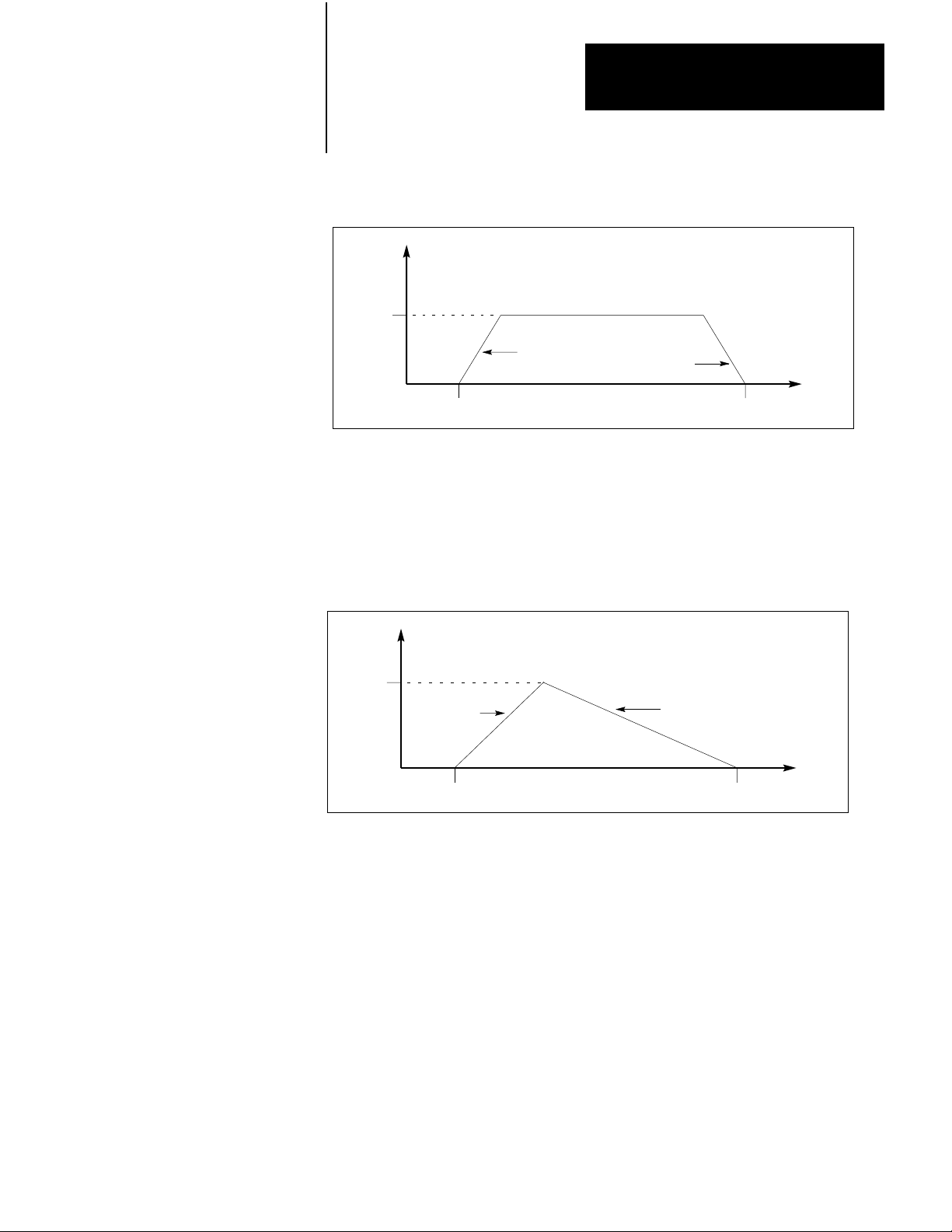
When the module receives a setpoint command, motion segment command, jog command, or a discrete jog input, it automatically calculates the velocity curve for the requested axis movement using parameters that you define for the move. (See Figure 3.2.)

32

Chapter 3

Positioning with the Linear Positioning Module

Figure 3.2 Trapezoidal

Velocity

Final Velocity

Axis Movement

Constant

Velocity

Acceleration

Start

0 Finish

Deceleration

Time

50002

The actuator may not reach the final velocity during a short move which may only consist of acceleration and deceleration phases without a constant velocity phase. This produces a ramp movement. (See Figure 3.3.)

Figure 3.3

Movement

Ramp

Velocity

Peak Velocity

Acceleration

Start

0 Finish

Deceleration

Time

50003

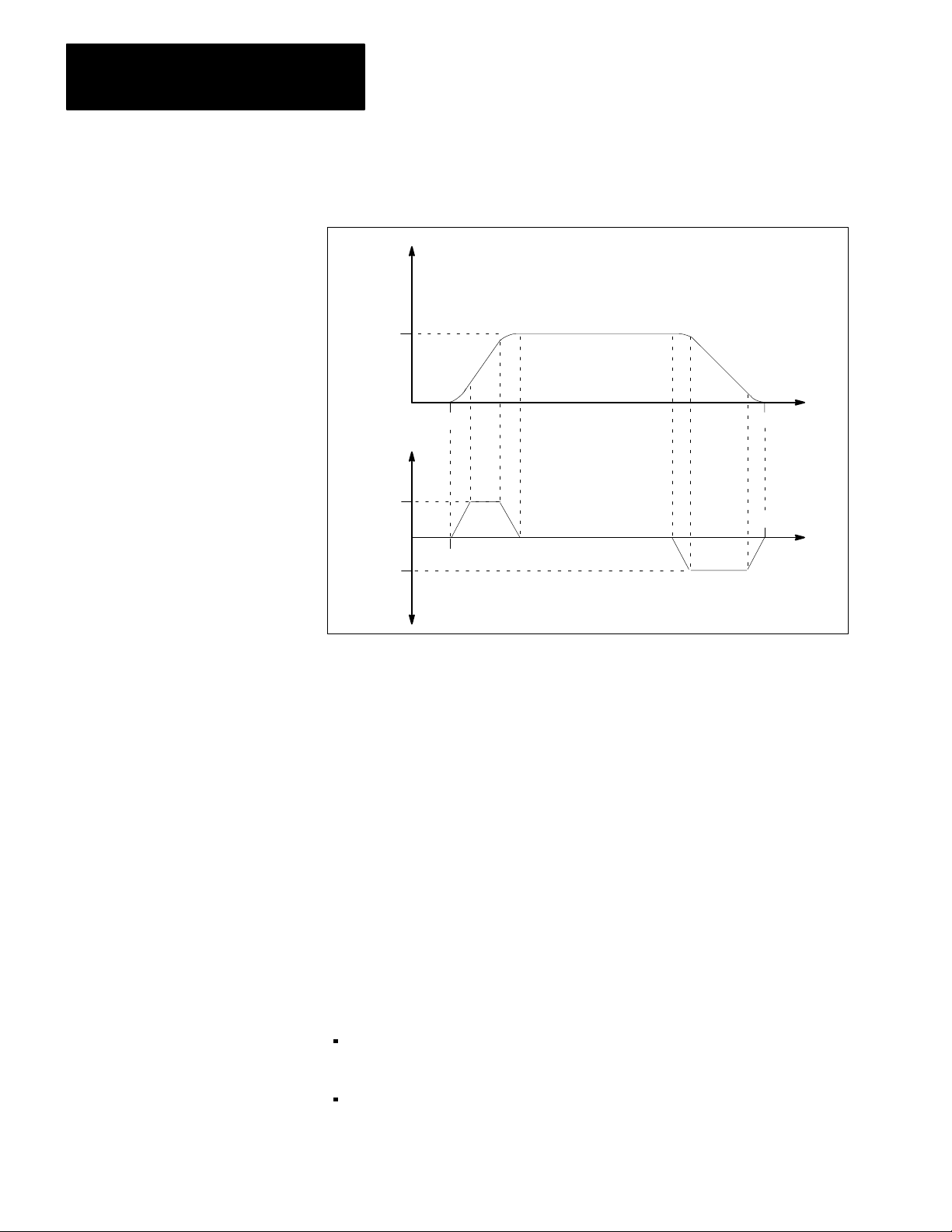
The module employs a technique called velocity curve smoothing to shape the velocity curve into an “S curve”. To achieve this smoothing, acceleration and deceleration rates are changed to provide more gradual application and removal of force, thus reducing mechanical wear. The velocity smoothing constant that you set in the parameter block determines how quickly acceleration and deceleration change. The lower the value of the velocity smoothing constant, the more slowly acceleration and deceleration change, producing a smoother transition. Figure 3.4 shows the effect of velocity curve smoothing on the axis movement.

33

Chapter 3

Positioning with the Linear Positioning Module

Figure 3.4

Movement with Velocity Curve Smoothing

Axis

Velocity

Final Velocity

Acceleration

Final Accel

Final Decel

Acceleration Deceleration

Start0 Finish

0

Start

Constant

Velocity

Time

Finish

Time

Commanding Motion

Deceleration

50004

There are three ways to specify module axis motion: by setpoints, by jogging or by motion blocks. All motion must be started using the command block and/or hardware inputs.

Setpoints

The module must have the axis controller in auto mode if you are using setpoint moves. You can switch between modes using the auto/manual bit in the command block or the auto/manual discrete input.

Important: The auto/manual bit and the auto/manual input must both be high to enter auto mode.

In the auto mode, you position the actuator by commanding desired setpoints using the command block. You can:

define up to 12 setpoints through the setpoint block. You can define the 13th

setpoint within the command block.

34

specify acceleration, deceleration, and velocity for each setpoint move.

Chapter 3

Positioning with the Linear Positioning Module

turn on a hardware start enable bit (using the command block), which causes

the module to delay movement to the commanded setpoint. The delay ends and movement starts when you activate the hardware start input or send a software start command in the command block.

command a setpoint while the axis is moving towards another setpoint. If the

new setpoint is in the opposite direction of travel, the axis decelerates to zero speed (at the current deceleration rate) and then moves in the opposite direction. If the new setpoint is in the same direction of travel, the old setpoint is abandoned and the axis movement accelerates or decelerates to the specified velocity and continues toward the new setpoint.

Jogging

In the manual mode, you position the actuator by jogging, i.e., directly commanding movement in one direction or the other. You make these movement commands by turning on forward or reverse jog bits (via the command block) or activating forward or reverse hardware jog inputs (typically via momentary action switches).

If you command a jog, the axis movement continues until the actuator reaches the software travel limit or until you turn off the jog bit or jog input, whichever occurs first.

Jog Rates

You define two jog rates (high and low) through the parameter block. You select between low and high jog rates through the jog rate select bit in the command block.

If you change jog rates (from high to low or from low to high) during a jog movement, the axis decelerates/accelerates to the new rate.

Important: Jog commands are ignored in auto mode.

Motion Blocks

A motion block contains information similar to that which the setpoint block uses to define axis movement. In addition, a motion block also contains trigger conditions that will initiate a subsequent axis movement, thus changing the motion of the axis without the intervention of the programmable controller. See Chapter 9 for a full explanation of motion blocks.

35

Chapter

4

Hardware Description

This chapter describes the Linear Positioning Module hardware, as well as other hardware required for a positioning system.

Indicators

Figure 4.1 shows the three indicators on the module.

Figure 4.1 Indicators

LINEAR

POSITIONING

FAULT

LOOP1 ACTIVE

LOOP2 ACTIVE

50009

When you first power up the module, all three indicators turn on for about one second. Next, the LOOP 1 ACTIVE and LOOP 2 ACTIVE indicators turn off while the module performs diagnostics. If the diagnostics discover a module fault, the red FAULT indicator stays on and the module remains inactive. When the programmable controller is in run mode, the indicators behave as follows:

FAULT - a red indicator that is normally off. The indicator turns on if there

is a module fault in one loop or both loops. See Chapter 11 for more information on module faults.

LOOP 1 ACTIVE - a green indicator that is on when loop 1 is active. The

indicator blinks if a fault occurs on loop 1 and turns off if loop 1 is inactive.

LOOP 2 ACTIVE - a green indicator that is on when loop 2 is active. The

indicator blinks if a fault occurs on loop 2 and turns off if loop 2 is inactive.

41

Chapter 4

Hardware Description

Wiring Arm Terminals

Transducer Interface

Discrete Inputs

Analog Outputs

Discrete Outputs

The module draws power for its internal circuitry and communicates with the programmable controller through the 1771 universal I/O chassis. You make all other connections through the wiring arm terminals. Cable length can be up to 200 feet for these connections, depending on the gauge used. See Chapter 5 for wiring guidelines. Figure 4.2 shows the wiring arm terminals for both control loops.

Figure 4.2

Arm T

+ GATE

- GATE

START

STOP

erminals

LINEAR

POSITIONING

FAULT

LOOP1 ACTIVE

LOOP2 ACTIVE

LOOP 1 + GATE

- GATE

+ INTERR

- INTERR +5 VDC

UNUSED

AUTO/MAN

START

STOP

JOG FWD

JOG REV

INPUT 1 INPUT 2

I/P SUPPLY

+ ANALOG

- ANALOG + 15 VDC

- 15 VDC

OUTPUT 1 OUTPUT 2

NO.

11 13 15 17 19 21 23 25 27 29 31 33 35 37 39

1 3 5 7 9

Transducer Interface

Discrete Inputs

Analog Outputs

Discrete Outputs

Wiring

NO.

2 4 6 8

+5 COMMON

10 12 14 16 18 20 22 24 26

I/P COMMON

28 30 32 34

± 15 COMMON

36 38 40

O/P SUPPLY

LOOP 2

+ INTERR

- INTERR

UNUSED

AUTO/MAN

JOG FWD

JOG REV

INPUT 1 INPUT 2

+ ANALOG

- ANALOG

OUTPUT 1 OUTPUT 2

42

50010

The input and output terminals of each of the module’s control loops are in four groups. Each group is electrically isolated from the 1771 backplane and from the three other groups:

transducer interface terminals

discrete input terminals

Chapter 4

Hardware Description

analog output interface terminals

discrete output terminals

The terminals for these four groups are divided between loop 1 and loop 2. Odd number terminals are for loop 1; even numbered terminals apply to loop 2.

Transducer Interface

Determining the Optimum Number of Circulations

Terminals 1 through 8 on the module’s wiring arm provide connection points for the transducer interface. The module is designed to work with the linear displacement transducers (LDT) listed in Chapter 1.

The transducer interface circuit is electrically isolated from the 1771 I/O chassis. This protects the 1771 backplane from noise and current surges in the transducer circuits. The transient isolation exceeds 1,500 volts RMS. The transducer interface is also isolated from the other module interfaces and external power supplies.

The module supports a transducer length of up to 15 feet (4572 mm), and can resolve the signal from the transducer to within two thousandths of an inch with one circulation. You can achieve a higher accuracy by configuring the transducer for more circulations. For example, the resolution for 60 inches (1524 mm) is better than one thousandth of an inch if two recirculations are used.

Every two milliseconds, the module sends an interrogate signal to the transducer. The transducer returns a pulse width that is proportional to the axis position. The maximum pulse width that can be measured without overflowing the counter is about 1680 microseconds (1.680 milliseconds).

The pulse width returned to the module depends on the transducer stroke length and the number of circulations. Each doubling of the number of circulations doubles the width of the gate pulse and the resolution of the position reading. Doubling the gate pulse length, however, effectively halves the maximum transducer length supported by the module, because the maximum pulse width is still determined by the size of the module’s counter. Overflowing the counter causes a feedback fault. Is is recommended that you configure the digital interface box for the highest number of circulations that still allows a long enough stroke length for your application. Increasing the number of circulations reduces the effect of noise and improves resolution.

43

Chapter 4

Hardware Description

Use these equations to determine the maximum length and positioning resolution for the transducer:

maximum length = 1680/(T x N) resolution = 1/(58.5 x T x N)

where:

T = transducer constant stamped on transducer head (typically

9.0500 microseconds per inch)

N = number of circulations

The following table gives several maximum transducer lengths assuming a transducer constant of 9.0500 microseconds per inch. Resolutions may be limited by the physical capabilities of the transducer. See Chapter 8 for a description of a procedure for verifying the transducer constant.

Number of

Circulations

1

2

3

4

5

6 0.0003 30.9

7 0.0003 26.5

8 0.0002 23.2

9 0.0002 20.6

10 0.0002 18.6

Resolution

(Inches)

0.002

0.001

0.0006

0.0005

0.0004

Maximum Transducer Length

(Inches)

185.6

92.8

61.9

46.4

37.1

Important: Apply a 10% to 20% margin when determining the maximum transducer length. The available stroke length will be less than indicated above due to the null space (typically 2 inches) near the transducer head.

44

Chapter 4

Hardware Description

Discrete Inputs

Terminals 13 through 26 on the module’s wiring arm provide connection points for discrete input signals. Seven terminals (for each loop) connect to seven discrete inputs.

The use of these inputs is optional. If you do not want to use them, you can disable them through the parameter block. (See Chapter 7.) If you disable the inputs:

the hardware stop input is deactivated (you do not have to tie it high)

the auto/manual input defaults to auto

the programmable controller programs can still read the status of the discrete

inputs in the status block

Because the programmable controller programs can still read the status of the discrete inputs, by disabling them you can redefine them for your own purposes.

Here are the requirements of the discrete inputs:

low signal 0 to 4 VDC

high signal 10.0 to 30.0 VDC

peak input current 8 mA at 12 VDC

16 mA at 24 VDC

The discrete inputs are configured as current sinks. To reduce heat dissipation, the module turns the discrete input currents off between samples at a 20% duty cycle every 2 ms.

Each discrete input has an internal pull-down resistor. If the device that you have connected to an input provides a high signal, the device must source current through the pull-down resistor. Figure 4.3 is a simplified schematic of a discrete input circuit.

45

Chapter 4

Hardware Description

Figure 4.3 Simplified

Schematic of a Discrete Input

1771 - QB MODULE

+ 5V

10K

3.3K

27

INPUT SUPPLY

DISCRETE INPUT (e.g. JOG FWD)

28

INPUT COMMON

50041

Auto/Manual Input

The module accepts the signal at the AUTO/MAN terminal (13/14) as the auto/manual input. Use this input in conjunction with block transfers to set the operation mode for the axis. A high input means auto mode and a low input means manual mode. The auto/manual input defaults to auto mode if the inputs are disabled via the parameter block.

Important: To set the mode of the axis to auto, you must set both the auto/manual input and the auto/manual bit in the command block high. If either the bit or the input is low, the mode is manual.

Hardware Start Input

In the auto mode, the module accepts a transition from low to high at the START terminal (15/16) as a high-true hardware start input signal.

If the axis is in auto mode, and if the hardware start has been enabled via the command block, the module waits for a transition from low to high at the START terminal before it will start axis movement to a previously commanded setpoint. If you don’t want to use this feature, disable the hardware start via the command block.

Important: Because of the module’s built-in switch debouncing, the low-to-high transition must follow a minimum 16 ms low signal.

46

Chapter 4

Hardware Description

Hardware Stop Input

The module accepts the signal at the STOP terminal (17/18) as a low-true hardware stop input. A low signal at the hardware stop input disables the analog output and stops axis movement. Unless the discrete inputs are disabled via the parameter block, this input must be high for normal operation. If the connection breaks, axis movement stops.

Example: If the loop fault output of one axis is connected to the hardware stop input of another axis, the movement of both axes will stop if a fault occurs.

Jog Forward Input

In manual mode, the module accepts a high signal at the JOG FWD terminal (19/20) as a high-true jog forward signal. When the module receives this signal, it moves the tool or workpiece forward until it reaches the software limit or until the input goes low. Forward is the direction of positive movement relative to the zero-position offset. Chapter 7 explains how to define the zero-position offset in the parameter block.

Analog Output Interface

Jog Reverse Input

In manual mode, the module accepts a high signal at the JOG REV terminal (21/22) as a high-true jog reverse signal. When the module receives this signal, it moves the tool or workpiece in the reverse direction until it reaches the software limit or until the input goes low. Reverse is the direction of negative movement relative to the zero-position offset.

Important: If the module detects a feedback fault, the jog inputs will perform open-loop jogs only. This means that the module can send velocity commands to the servo valve (at the low jog rate), but can’t monitor axis position. Therefore, software travel limits are ignored.

General Purpose Inputs

There are two general purpose inputs for each control loop of the module at terminals INPUT 1 (23/24) and INPUT 2 (25/26). You can monitor the state of the signal at these terminals through the status block. These inputs can also be configured as programmable as described in Chapter 9.

The module’s analog outputs, terminals 29 through 32, connect to a hydraulic valve for each axis that the module controls. These outputs supply up to + mA for direct servo valve control or up to + amplifiers or other voltage controlled devices.

10 V for proportional valve

100

47

Chapter 4

Hardware Description

The analog output interface circuit is electrically isolated from the 1771 I/O chassis. This feature protects other devices on the 1771 backplane from noise and current surges in the analog output circuit. An internal relay automatically shuts off these outputs in the event of a module fault. For details on connecting the servo valve interface, see Chapter 5.

Important: Throughout this manual we refer to servo valves, but you can also use the analog outputs to control proportional valves. All references to servo valves also apply to proportional valves.

Discrete Outputs

Terminals 36 through 39 on the module’s wiring arm provide connection points for discrete output signals. Each axis has two discrete outputs: Output 1 which can be configured to be either an in-position or programmable output, and Output 2 which can be configured to be either a loop fault or programmable output. (See Chapter 9.) The default configuration is in-position and loop fault. The discrete outputs are current sources. Figure 4.4 gives a simplified schematic of a discrete output circuit.

Figure 4.4 Simplified

Schematic of a Discrete Output

1771  QB MODULE

3.9

40

OUTPUT SUPPLY

37

OUTPUT 1

48

Here are the characteristics of the discrete outputs:

Low no voltage applied to the output

High output supply voltage applied to output

Maximum Current 100 mA

Voltage Drop 1.6 VDC maximum (at 100 mA) between the

discrete output power supply (terminal 40) and the discrete outputs

5 0 0 4 2

50042

Chapter 4

Hardware Description

Important: If you want to connect a discrete output of one axis to the discrete input of another axis, the minimum discrete output supply voltage is 11.6 VDC. This accounts for the voltage drop of 1.6 VDC shown above and provides the minimum voltage required to drive a module discrete input (10 VDC).

ATTENTION: The discrete outputs can withstand a short circuit for a few seconds. However, a continuous short circuit will damage the module’s discrete output transistor.

OUTPUT 1

When OUTPUT 1 (terminals 36/37) is configured as an in-position output, it turns off when axis movement toward a commanded endpoint begins and turns on when the axis enters the in-position band (defined in the parameter block). You can connect an in-position output to a hardware start input to provide a simple form of axis coordination.

Power Supplies

When this output is configured as a programmable output, its state is determined by the configuration information provided in the motion blocks. (See Chapter 9.)

OUTPUT 2

When OUTPUT 2 (terminal 38/39) is configured as a loop fault output, it is high under normal axis operation. When the module detects a fault in the axis, the loop fault output goes low.

You can connect the loop fault output to the hardware stop input of other control loops so all axis movement will stop if a fault occurs. The loop fault output then provides the low signal required by the hardware stop input of the other axis.

As with OUTPUT 1, OUTPUT 2 can be configured as a programmable output and its state determined by information in the motion blocks.

You must provide external DC power for the input and output circuits. You could use a single supply, but you’ll maintain maximum separation and keep noise to a minimum by using four separate power supplies. In less critical applications, you could power two or three circuits from the same supply.

49

Chapter 4

Hardware Description

to power the: supply:

Transducer interface +5 VDC 9, 10

Discrete inputs +24 VDC (max) 27, 28

Servo valve interface +15 VDC 33, 34, 35

Discrete outputs +30 VDC (max) 40

to these terminals:

All power connections must be made for the transducer, servo valve, and discrete outputs. The power supply for discrete inputs may be left unconnected if the discrete input disable bit has been set in the parameter block.

410

Chapter

5

Installing the Linear Positioning Module

Before You Begin

This chapter tells you how to install the module in the I/O chassis and how to configure the module’s analog outputs by setting DIP switches. Before you install the module:

make sure your power supply is adequate

plan your module’s location in the I/O chassis

take steps to avoid electrostatic discharge

Avoiding Backplane Power Supply Overload

Make sure your power supply can handle the extra load before installing the module in your I/O chassis. Add the module’s current requirement, listed on the module’s label, to the currents required by other modules inserted in the I/O chassis. If the backplane power supply rating is less than the total current required, you’ll need a larger power supply.

Here are the current ratings for the various Allen-Bradley power supply modules.

This Power Supply Module:

Is Rated at:

1771P1

1771P2

1771P4 8A

1771P5

1771P7

6.5A

8A

16A

Planning Module Location

The module requires one I/O chassis slot. You can install it in any slot in the I/O chassis. The module uses both the output image table byte and the input image table byte that corresponds to its location address.

51

Chapter 5

Installing the Linear Positioning Module

Electrostatic Discharge

Under some conditions, electrostatic discharge can degrade performance or damage the module. Observe the following precautions to guard against electrostatic damage:

use a static-free workstation if one is available

touch a grounded object to discharge yourself before handling the module

don’t touch the backplane connector or connector pins

when you set the analog output switches, don’t touch other circuit

components inside the module

keep the module in a static-shielded bag when it’s not in use

Setting Analog Output Switches

You set the analog output DIP switches to define the range of output voltage or output current for the analog output of each control loop.

There are two switch assemblies for each control loop: a single switch assembly that selects voltage or current output and a dual switch assembly that sets the current range. The current range switch has no effect if you choose a voltage output. You must limit the voltage range through the analog range word in the parameter block if you require a voltage range of less than + Chapter 7.)

If the analog output will be controlling a current controlled device, such as a servo valve, set the single switch for current and set the current range to match the device. If your device requires a range that falls between those provided, select the next higher range and reduce the range using the analog range word in the parameter block.

Important: Although you can set the current range with the analog range word in the parameter block, you’ll improve analog output resolution by first limiting the range with the current range DIP switch.

To set the switches:

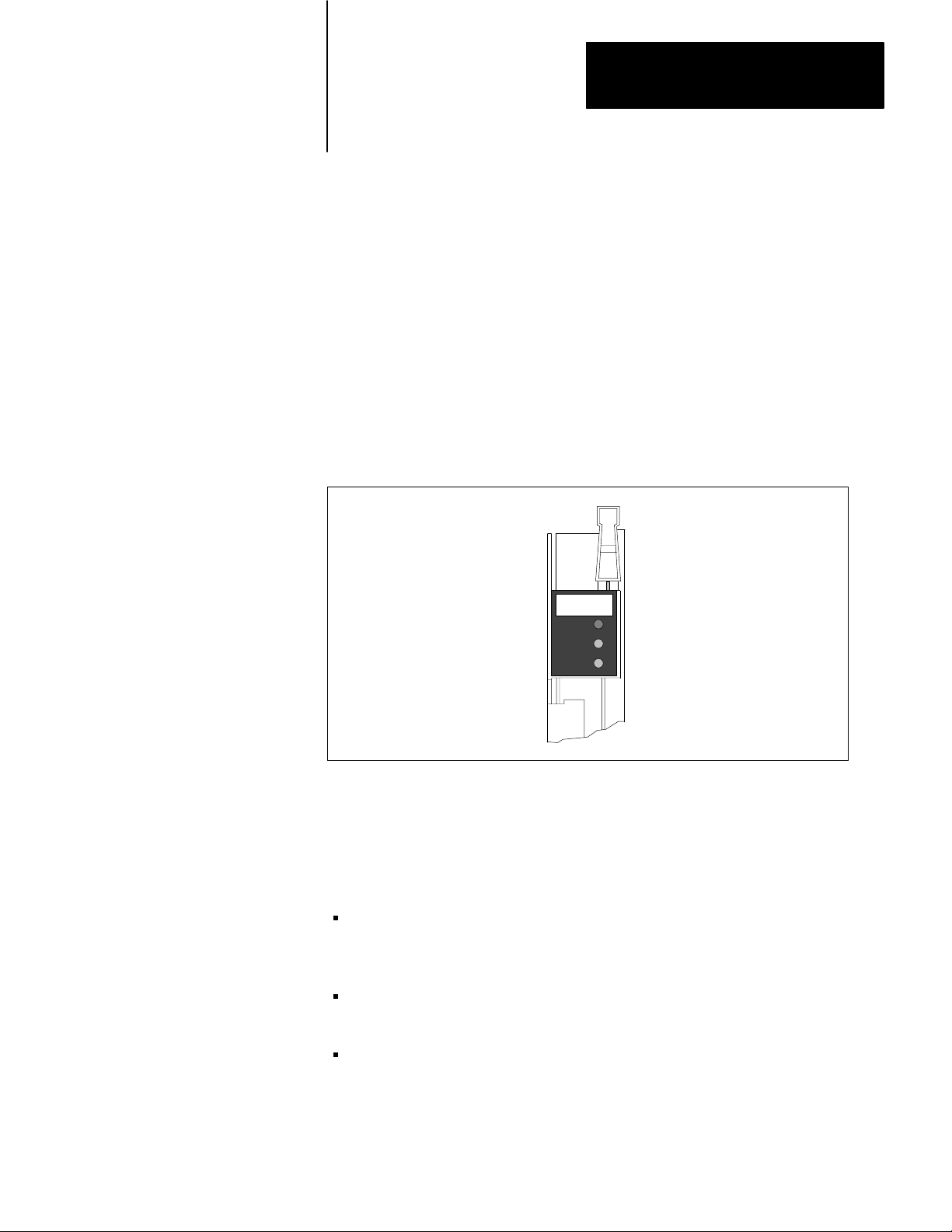
1. Lay the module on its side and locate the switches using Figure 5.1. All

switches are accessible from the right edge of the module without removing the module cover.

10 VDC. (See

52

Chapter 5

Installing the Linear Positioning Module

Figure 5.1 Locating

the Analog Configuration Switches

LOOP 2

LOOP 1

CURRENT RANGE VOLTAGE/CURRENT

2. Use a blunt pointed instrument (such as a ballpoint pen) to set the

switches.

ATTENTION: Don’t use a pencil to set switches. Lead can jam the switch.

50043

53

Chapter 5

Installing the Linear Positioning Module

3. Set the current/voltage switch for each control loop as shown in

Figure 5.2.

Figure 5.2 Configuring

SLIDEONROCKERONTOGGLE

the Analog Outputs

TYPES OF SWITCHES

ON

C1

12

C2

±100mA

± 50mA

± 20mA

LOOP 1

1 2

OPEN

12

C2

12

C2

12

C2

C1

LOOP 2

C1

12

C2

1 2

OPEN

2

1

OPEN

2

1

OPEN

1 2

1771QB Chassis

54

2

C1

1

2

C2

1

OPEN

± 10V

The range selection switches have no

effect when ±10V is selected.

50044

4. If you have selected a current output, set the current range switch to +100

mA, +

50 mA, or +20 mA as shown in Figure 5.2. If your device requires a range that falls between those provided, select the next higher range and reduce the range using the analog range word in the parameter block.

ATTENTION: If your switch setting does not provide enough current, the servo valve may not operate to its full capability. On the other hand, excessive currents may damage the servo valve.

Chapter 5

Installing the Linear Positioning Module

Keying

A package of plastic keys (Cat. No. 1771-RK) is provided with every I/O chassis. When properly installed, these keys prevent the seating of anything but the module in the keyed I/O chassis slot. Keys also help to align the module with the backplane connector.

Each module is slotted at its rear edge. Position the keys on the chassis backplane connector, corresponding to the slots on the module’s rear edge.

Insert the keys into the upper backplane connectors. Position the keys between the numbers at the right of the connectors, as shown in Figure 5.3.

Figure 5.3

Keying

Module

2 4 6 8 10 12

Keying Positions

Between

D pins 16 and 18 D pins 30 and 32

14 16 18 20 22 24 26 28 30 32 34 36

Inserting the Module

50045

After setting analog output switches and setting the keying positions, you’re ready to insert the module into a slot in the I/O chassis.

To insert the module, follow this procedure:

1. Remove all power from the I/O chassis and from the module’s wiring arm

before inserting or removing a module.

55

Chapter 5

Installing the Linear Positioning Module

2. Open the module locking latch on the I/O chassis and insert the module

into the slot keyed for it.

3. Press firmly to seat the module into the backplane connector.

4. Secure the module with the module locking latch.

ATTENTION: Don’t force a module into the backplane connector.

If you can’t seat a module with firm pressure, check the alignment and keying. Forcing a module can damage the backplane connector and the module.

Wiring Guidelines

Through the module’s terminals, you connect the module to external devices. The exact wire gauge and maximum allowable length depends upon the devices being connected. Here are some general rules to follow when you connect the terminals:

don’t use wire with too large a gauge. The maximum practical wire gauge is

14 AWG.

keep low level conductors separate from high level conductors. Follow the

practices outlined in Publication 1770-980 P2LC Grounding and Wiring Guidelines.

keep your power supply cables as short as possible–less than 50 feet is

preferable.

Using Shielded Cables

For many connections, you are instructed to use shielded cables. Using shielded cables and properly connecting their shields to ground protects against electromagnetic noise interfering with the signals transmitted through the cables. Connect each shield to ground at one and only one end. At the other end, cut the shield foil and drain wire short and cover them with tape. This will protect them against accidentally touching ground. Keep the length of leads extending beyond the shield as short as possible.

56

Figure 5.4 shows shielded cable connections for one control loop. Mount a ground bus directly below the I/O chassis to provide a connection point for the cable shield drain wires and the common connections for the input and output circuits. Connect the I/O chassis ground bus through 8 AWG wire to the central ground bus to provide a continuous path to ground.

Chapter 5

Installing the Linear Positioning Module

Transducer Supply

Figure 5.4 Shielded

4

Cable Grounding Connections

5

LINEAR

POSITIONING

FAULT

LOOP1 ACTIVE

LOOP2 ACTIVE

Transducer

1

2

Discrete

2

Input

Supply

3

Analog Supply

Discrete

Output

Supply

2

5

2

Shielded cables are not required for these discrete inputs and outputs. However, they can improve noise immunity.

I/O Chassis Ground Bus

8 AWG wire to central ground bus

1

Belden 8723 or equivalent (50 ft. max.), Belden 8227, Belden 9207, Belden 1162A, or equivalent (200 ft. max.)

2

Belden 8761 or equivalent (50 ft. max.)

3

Belden 8761 or equivalent (200 ft. max.)

4

Belden 8761 or equivalent (25 ft. max.), Belden 9318 or equivalent (50 ft. max.)

5

Belden 8723 or equivalent (50 ft. max.)

Servo Valve

50026

57

Chapter 5

Installing the Linear Positioning Module

Using Twisted Wire Pairs

It is recommended you use twisted wire pairs for a signal and its return path to reduce noise levels further. Figure 5.5 shows a twisted pair and shielded twisted pair.

Figure 5.5 Shielded

T

wisted Pair Diagram

Twisted Pair

Shielded Twisted Pair

50046

ATTENTION: Failure to follow correct shielding procedures can cause unpredictable movement resulting in possible injury to personnel and damage to equipment.

Connecting AC Power

Figure 5.6 shows AC power and ground connections. Incoming AC connects to the primary of an isolation transformer. The secondary of the isolation transformer connects to:

58

the power supply for the discrete inputs

the power supply for the discrete outputs

the power supply for the I/O chassis

the power supply for the analog outputs

the power supply for the transducer circuits

Disconnect

Figure 5.6

Power and Ground Connections

AC

L3

Chapter 5

Installing the Linear Positioning Module

Incoming

AC

L1 N

Power

Supply for

Discrete

Inputs

L2

L1

Fuses

H

1

H

3

Fuse

G

120 VAC

L1 N

Power

Supply for

Discrete Outputs

G

X

1

Ground Bus

Supply for

I/O Chassis

Backplane

H

2

X

2

Central

L1 N

Power

4

Isolation/ StepDown Transformer

L1 N

Power

G

Supply for

Analog

Outputs

G

L1 N

Power

Supply for

Transducer

Circuits

G

I/O Chassis Ground Bus

50047

In the grounded AC system shown above, the low side of the isolation transformer is connected to the central ground bus. Figure 5.6 also shows connections from the central ground bus to each power supply and to the I/O chassis ground bus shown in Figure 5.4.

59

Chapter 5

Installing the Linear Positioning Module

Power Supplies

The 1771 backplane provides the power for most of the module circuits. You’ll need external power supplies for the analog outputs, transducer interfaces, discrete inputs and discrete outputs.

All four power supplies and their associated module circuits are electrically isolated from the I/O chassis and from each other. To provide maximum isolation of the four sets of circuits, the four supplies should be from separate sources. However, you can use the same power supply to power two or more circuits if you don’t need the isolation that separate supplies provide.

Information on how to connect the power supply for each circuit is under the heading for that circuit.

Connecting the Transducer Interface

Figure 5.7 shows the transducer interface connections. You should refer to the wiring diagrams supplied with your transducer to determine pinouts on the transducer head.

Important: The transducer must be configured for external interrogation.

510

Chapter 5

Installing the Linear Positioning Module

LOOP 2

TRANSDUCER

Figure 5.7 Transducer

Connections

Connect to

Transducer Head

55

- + +5 Com

Transducer

Supply

(Customer Supplied)

LOOP 1

TRANSDUCER

4

Ground the shield at

the I/O chassis end.

Wiring Arm

Terminals

1

Ground the shield

at the I/O chassis end.

1

Belden 8723 or equivalent (50 ft. max.); Belden 8227, Belden 9207, Belden 1162A or equivalent (200 ft. max.)

4

Belden 8761 or equivalent (25 ft. max.), Belden 9318 or equivalent (50 ft. max.)

5

Belden 8723 or equivalent (50 ft. max.)

2 4 6 8

+5 COMMON

10

LOOP 2

+GATE

-GATE

+INTERR

-INTERR

LOOP 1

+GATE

-GATE

+INTERR

-INTERR +5 VDC

1 3 5 7 9

Ground the shield

at the I/O chassis end.

Power Supply

To connect the transducer power supply, follow these steps:

1. Connect +5 VDC from your power supply to the +5 VDC terminal (9) on

the module.

1

50030

2. Connect + VDC from your power supply to the transducer.

511

Chapter 5

Installing the Linear Positioning Module

3. Connect - VDC from your power supply to the transducer.

4. Connect the common terminal on your power supply to the +5 COMMON

terminal (10) on the module, to ground at the I/O chassis, and to the transducer.

5. Connect the cable shields to ground at the I/O chassis end.

6. Connect the power supply chassis to ground.

Transducer Interface

After connecting the transducer power supply to the module, make the Gate and Interrogate connections. Use a single, continuous, shielded cable segment for these connections. Don’t break the cable for connection in a junction box, but connect it directly from the digital interface box to the module.

To connect the transducer interface terminals:

1. Configure the transducer for external interrogation.

2. If you haven’t already configured the transducer for the optimum number

of circulations, do so now. Refer to Chapter 4 for a procedure to determine the optimum number of circulations for your system.

3. Connect the module’s +GATE terminal (1/2) to the transducer’s +GATE

terminal.

4. Connect the module’s -GATE terminal (3/4) to the transducer’s –GATE

terminal.

5. Connect the module’s +INTERR terminal (5/6) to the transducer’s

+INTERROGATE terminal.

6. Connect the module’s -INTERR terminal (7/8) to the transducer’s

–INTERROGATE terminal.

7. Connect the cable shields to ground at the I/O chassis end.

Connecting the Discrete Inputs

512

The seven discrete inputs (for each control loop) make connections via eight wiring arm terminals (one terminal is discrete input common). The voltage and current requirements for the discrete inputs are:

Low 0 to 4 VDC

High 10 to 30 VDC

Input Current 8 mA @ 12 VDC

16 mA @ 24 VDC

Chapter 5

Installing the Linear Positioning Module

Make sure that the voltage driving each input is at the appropriate level. Figure 5.8 shows the discrete input connections.

Auto/Manual

Start

Use any number of

Estop switches in series

Jog Forward

Jog Reverse

Input 1

Input 2

Figure 5.8 Discrete

2

14

AUTO/MAN

16 18 20 22 24 26 28

I/P COMMON

Input Connections

LOOP 2

START

STOP JOG FWD JOG REV

INPUT 1 INPUT 2

Wiring Arm

Terminals

LOOP 1

AUTO/MAN

START

STOP JOG FWD JOG REV

INPUT 1 INPUT 2

I/P SUPPLY

13 15 17 19 21 23 25 27

Auto/Manual

Start

Use any number of

2

Estop switches in series

Jog Forward

Jog Reverse

Input 1

Input 2

15 to 24 VDC

Discrete Input

Supply

(Customer

Supplied)

- +

2

Belden 8761 or equivalent (50 ft. max.)

50049

If you are driving a discrete input from a discrete output of another module, keep in mind that you must measure the output voltage at the discrete output itself and not at the discrete output power supply. There is a 1.6 VDC drop between the power supply and the discrete output at maximum current. To yield the minimum 10 VDC at the discrete output, the discrete output supply must be greater than 11.6 VDC.

513

Chapter 5

Installing the Linear Positioning Module

Power Supply

To connect the discrete input power supply, follow these steps:

1. Connect the (+) side of the discrete input power supply to the I/P SUPPLY

terminal (27) of the module.

2. Connect the common of the discrete input power supply to the I/P

COMMON terminal (28) of the module.

3. Connect the cable shield to ground at the I/O chassis end.

4. Connect the power supply chassis to ground.

Auto/Manual Input

The auto/manual input, in conjunction with the auto/manual bit in the command block, determines the module’s mode of operation. Both the auto/manual input and the auto/manual bit must be on to achieve auto mode. Otherwise, the mode is manual. Connect the auto/manual and common terminals to an external source.

Hardware Start Input

The hardware start input performs the same function as the software start. (See Chapter 8.) When you command a setpoint, no axis movement occurs on that control loop until the module receives a start command or a transition from low to high (after at least 20 msec of low) at the control loop START terminal (15/16).

Example: To start movement to a setpoint when Output 1 (configured as the in-position output) of another control loop goes high, connect the hardware start input to the Output 1 of that control loop.

You don’t need to connect the hardware start terminals if you won’t be using this feature.

514

Hardware Stop Input

A low input at the STOP terminal (17/18) will stop axis movement for the corresponding control loop. This allows you to connect any number of normally closed emergency stop switches in series between a high source and the hardware stop terminal. Opening any of these switches will immediately zero the analog output for that loop.

Chapter 5

Installing the Linear Positioning Module

ATTENTION: In servo valve control systems, axis drift may occur due to imprecise valve nulling even with zero analog output. It is recommended that emergency stop switches, such as overtravel limit switches, also turn off axis power and close a blocking valve installed between the servo valve and the prime mover.

Important: If you have enabled the discrete inputs via the parameter block, don’t leave the hardware stop terminals disconnected–you must connect them to a source which is normally high. If the connection breaks, the input goes low and axis movement automatically stops.

ATTENTION: Use the hardware stop to disable the servo valve drive or stop axis motion only in an emergency. Abruptly stopping axis motion places mechanical stress on the positioning assembly. Use the slide stop bits in the command block to stop axis motion in non-emergencies. The slide stop decelerates before stopping and is less abrupt than the hardware stop.

Jog Forward Input

Before the module responds to the jog forward input, the control loop must be in manual mode.

If you apply high input (more than 10 VDC) to the jog forward input, the axis moves in the forward direction (the direction of positive movement relative to the zero-position offset). It continues to move until the jog forward input is low or until the axis reaches the software travel limit, whichever occurs first.

Chapter 8 explains how to define the zero-position offset in the parameter block.

To set up the jog forward input:

1. Connect a normally open push-button switch between the JOG FWD input

terminal (19/20) and the discrete input power supply’s positive terminal (27).

2. Mount the jog forward switch so an operator can see the axis motion.

Leave the jog forward input terminal disconnected if you’re not using it.

515

Chapter 5

Installing the Linear Positioning Module

Jog Reverse Input

The jog reverse input is valid only in the manual mode. The jog reverse input is similar to the jog forward input, except the axis movement is in the reverse direction (the direction of negative movement relative to the zero-position offset). Connect the JOG REV terminal (21/22) in the same way as the jog forward input. Leave the terminal disconnected if you are not using it.

General Purpose Inputs

There are two general purpose inputs for each control loop of the module at terminals INPUT 1 (23/24) and INPUT 2 (25/26). You can monitor the state of the signal at these terminals through the status block (see Chapter 6) or use these terminals as programmable inputs (see Chapter 9).

Connecting Multiple Modules

To connect the discrete inputs of two or more modules to a single control line, you must pull the signal to ground with either a double-throw switch or a pull-down resistor.

Figure 5.9

a DoubleThrow Switch to Control Multiple QB'

Using

10 to 30 VDC

Doublethrow

Switch

14 16 18 20 22 24 26

28

14 16 18 20 22 24 26

28

s

LOOP2

AUTO/MAN

START

STOP

JOG FWD

JOG REV

INPUT 1 INPUT 2

I/P COMMON

LOOP2

AUTO/MAN

START

STOP

JOG FWD

JOG REV

INPUT 1 INPUT 2

I/P COMMON

Module A

Wiring Arm

Module B

Wiring Arm

516

50025

Chapter 5

Installing the Linear Positioning Module

Pull-down resistors or double-throw switches are only required if you wish to connect two or more QB’s. They are not required to control multiple discrete inputs on a single module.

Figure 5.10 Using

PullDown Resistors to Control Multiple QB'

10 to 30 VDC

Jog Reverse

Jog Forward

PullDown Resistors 1000 W 2W

s

14 16 18 20 22 24 26

28

LOOP2

AUTO/MAN

START

STOP

JOG FWD

JOG REV

INPUT 1 INPUT 2

I/P COMMON

Module A

Wiring Arm

PullDown Resistors 1000 W 2W

14 16 18 20 22 24 26

28

14 16 18 20 22 24 26

28

LOOP2

AUTO/MAN

START

STOP

JOG FWD

JOG REV

INPUT1 INPUT 2

I/P COMMON

LOOP2

AUTO/MAN

START

STOP

JOG FWD

JOG REV

INPUT 1 INPUT 2

I/P COMMON

Module B

Wiring Arm

Module C

Wiring Arm

50024

ATTENTION: Failure to follow these procedures can result in sporadic operation of the discrete inputs.

517

Chapter 5

Installing the Linear Positioning Module

Connecting the Analog Outputs

A B

C D

3

The analog outputs provide the current (or voltage) by which the module controls the servo valve. By controlling the servo valve, the module controls axis motion.

Figure 5.11 Analog

LOOP 2

SERVO VALVE

ATTENTION: Applying output to an axis with polarity reversed can cause sudden high-speed motion. For maximum safety, leave the analog outputs disconnected and the axis power off until you perform the axis tuning procedures in Chapter 8.

Output Connections

LOOP 1

SERVO VALVE

A B

C D

3

Ground the shield at the I/O chassis end.

Ground the common at the I/O chassis end.

LOOP 2

+ANALOG

30

-ANALOG

32 34

±15 COMMON

Ground the shield at the I/O chassis end.

3

Belden 8761 or equivalent (200 ft. max.)

5

Belden 8723 or equivalent (50 ft. max.)

Wiring Arm

Terminals

± 15 VDC

Analog Power

Supply

(Customer Supplied)

+ Comm -

+15 -15

5

LOOP 1

+ANALOG

-ANALOG +15 VDC

-15 VDC

29 31 33 35

Ground the shield at the I/O chassis end.

50031

518

Chapter 5

Installing the Linear Positioning Module

ATTENTION: The polarity of the analog outputs is affected by the setting of the most significant bit of the analog range words in the parameter block. (See Chapter 7.) Incorrect wiring of the analog outputs or an incorrect setting of this most significant bit can cause the axis to accelerate out of position when the loop is closed.

Power Supply

To connect the analog output supply:

1. Connect the (+) side of the power supply to the +15 VDC module terminal

(33).

2. Connect the (-) side to the -15 VDC module terminal (35).

3. Connect the common to +

ground at the I/O chassis.

4. Connect the shield to ground at the I/O chassis end.

5. Connect the analog power supply chassis to ground.

15 COMMON module terminal (34) and to

Analog Output

To connect the analog output of the control loop to the servo valve interface:

1. Be sure that you set the control loop’s voltage/current selection switches to

match your servo valve’s requirements.

2. Check that the analog output power supply is connected.

3. Connect the +ANALOG module terminal (29/30) and the -ANALOG

module terminal (31/32) to the servo valve coil terminals.

Important: If you select voltage output for a loop, the module internally connects that loop’s -ANALOG terminal to the +

15 COMMON terminal (34).

4. Connect the cable shields to ground at the I/O chassis end. Important: Wire servo valve coils in series. Refer to the instructions for your

device.

519

Chapter 5

Installing the Linear Positioning Module

Connecting the Discrete Outputs

2

The two discrete outputs for each loop are powered by the discrete output power supply. The characteristics of the discrete outputs are:

Low no voltage applied to the output

High output supply voltage applied to output

Maximum Current 100 mA

Voltage Drop 1.6 VDC maximum (at 100 mA) between the dis

crete output power supply (terminal 40) and the discrete outputs

Power for the OUTOUT 1 and OUTPUT 2 discrete outputs comes from the discrete output power supply through terminal 40 on the module wiring arm. The return for the load driven by OUTOUT 1 or OUTPUT 2 connects to the common of the discrete output power supply.

Figure 5.12 shows a typical discrete output connection.

Figure 5.12 Discrete

36 38 40

Output Connections

LOOP 2

OUTPUT 1 OUTPUT 2

O/P SUPPLY

Wiring Arm

Terminals

LOOP 1

OUTPUT 1 OUTPUT 2

37 39

2

520

LOADS*

Ground the shield at the I/O chassis end.

2

Belden 8761 or equivalent (50 ft. max.)

LOADS*

5 to 30 VDC

Discrete Output

Supply

(Customer Supplied)

+ -

2

*The discrete outputs can be connected to inputs of other modules provided that the current does not exceed 100mA.

50050

Chapter 5

Installing the Linear Positioning Module

Power Supply

To connect the discrete output power supply, follow these steps:

1. Connect the (+) side of the discrete output power supply to the O/P

SUPPLY terminal (40) on the module.

2. Connect the common of the discrete output power supply to ground at the

I/O chassis and to the returns (-) of all output devices.

3. Connect the discrete output power supply chassis to ground.

4. Connect the shield to ground at the I/O chassis end.

OUTPUT 1

If configured as an in-position output, this output goes low in auto mode when the axis begins to move towards a commanded setpoint or after a jog. It goes high when the axis enters the in-position band surrounding an endpoint.

You can use this output to drive another control loop to coordinate the axis movement of various control loops. In this case, you connect the OUTPUT 1 terminal to the discrete hardware start input of another control loop. Otherwise, you may connect this output to a light emitting diode or other indicator.

Important: When you are connecting the module’s discrete inputs and outputs to external devices, keep in mind that the discrete inputs sink current and the discrete outputs source current.

OUTPUT 2

If configured as a loop fault output, this output is normally high. It goes low when the module detects a fault in the control loop. You can use the loop fault output to drive another module’s hardware stop input. You can connect the loop fault output terminal to the hardware stop input of another control loop or to a visual/audible fault indicator.

Both OUTPUT 1 and OUTPUT 2 can be configured to be programmable outputs. (See Chapter 9.)

521

Chapter 5

Installing the Linear Positioning Module

36 38 40

LOOP 2

OUTPUT 1 OUTPUT 2

O/P SUPPLY

Wiring Arm

Terminals

Figure 5.13 Connecting

LOOP 1

OUTPUT 1 OUTPUT 2

a Discrete Output to a Discrete Input

LOOP 2

14

AUTO/MAN

16 18 20 22 24 26 28

I/P COMMON

START

STOP

JOG FWD

JOG REV

INPUT 1 INPUT 2

37 39

15 to 24 VDC

Supply

(Customer

Supplied)

+ -

Wiring Arm

Terminals

LOOP 1

AUTO/MAN

START

STOP

JOG FWD

JOG REV

INPUT 1 INPUT 2

I/P SUPPLY

13 15 17 19 21 23 25 27

Ground the shield at the I/O chassis end.

Important: Ground the power supply common at one point only. This will help

eliminate ground loops which are very susceptible to electrical noise.

50051

522

Chapter

6

Interpreting ModuletoPLC Data (READS)

This chapter explains how to monitor module operation from a programmable controller by reading and interpreting status block data that the module transfers to the programmable controller’s data tables.

PLC Communication Overview

You must program the programmable controller to communicate with the Linear Positioning Module through block read and block write instructions. The data blocks are:

status block

parameter block

setpoint block

motion block

command block

The block read instruction transfers the status block data from the module to the programmable controller data table. The block write instruction transfers the parameter block, the setpoint block, the motion block and the command block data from the programmable controller data table to the module. This chapter tells you how to interpret the status block data. Chapter 7 tells you how to format the parameter block, the setpoint block, and the command block data. Chapter 9 explains the motion block.

Status Block

The status block contains information on the status of each axis. Until the module receives a parameter block, the status block consists of five words (i.e. the default assumption of one axis). The size of subsequent status blocks depends on the configuration you program through the parameter block.

Number of Axes Status Block Length

1 5 words - default

2 9 words - default

1 or 2 up to 33 words depending on

block transfer length requested

You can set the block transfer read instruction to include extended status information by specifying a block transfer length of 33. If you specify a length of 0 (or 64), the module returns the default: 5 words for one axis and 9 for two.

61

Chapter 6

Interpreting ModuletoPLC Data (READS)

Word Assignment

The assignment of the words within the status block is as follows:

Figure 6.1

Block W

Status

AXIS 1 AXIS 2

ord Assignments

WORD DESCRIPTION

1 2 3 4 5

10 12 13 16 17 20 22 24 26 28 30 32

(6) (7) (8) (9)

(11) (14) (15) (18) (19) (21) (23) (25) (27) (29) (31) (33)

Module Configuration Word Status word 1 Status word 2 (MS) Position/Error/Diagnostic word (LS) Position/Error/Diagnostic word

Active motion segment/setpoint (MS) Position (LS) Position (MS) Following Error (LS) Following Error Measured Velocity Desired Velocity Desired Acceleration Desired Deceleration % Analog Output Maximum Positive Velocity Maximum Negative Velocity

Default Status

Extended Status

50000

Module Configuration Word (word 1)

Bits 0 to 8 are controlled by the parameter control word in the parameter block. Module configuration information includes number of axes, units of measurement, number format, binary position format (single or double word), and the state (enabled or disabled) of the start/stop enhancement, discrete input, analog output and transducer interface bits. Detailed descriptions of these are in Chapter 7.

62

Chapter 6

Interpreting ModuletoPLC Data (READS)

Figure 6.2

Configuration W

Module

15 14 13 12 11 10 09 08 07 06 05 04 03 02 01 00

.

. . . . .

0

. .. .

.

0

0000 0

.

..

.

Stop/Start Enhancement: 0 = Disabled 1 = Enabled

Binary Position Format: 0 = Double Word 1 = Single Word

ord

.

. . . . . . .. .

Transducer Interface: 0 = Enabled 1 = Disabled

.

..

.

Analog Outputs: 0 = Enabled 1 = Disabled

.

. . . . . . .. .

.

..

.

. . . . . . .. .

Format: 0 = Binary 1 = BCD

Discrete Inputs: 0 = Enabled 1 = Disabled

.

..

.

Axes used: 01 = Axis 1 10 = Axis 2 11 = Both axes

Units: 0 = Inch 1 = Metric

50001

Status Word 1 (words 2 and 6)

Each bit in status word 1 corresponds to a particular axis condition.

Bit 0 – Ready

The module turns off the ready bit after powerup or after a reset command. (See Chapter 7.) The module turns this bit on when it receives a valid parameter block for this loop. Unless it detects a fault, the module enables the analog output for the axis when the ready bit turns on.

The module does not accept setpoint, motion or command blocks until the ready bit is on.

63

Chapter 6

Interpreting ModuletoPLC Data (READS)

15 14 13 12 11 10 09 08 07 06 05 04 03 02 01 00

. . . . . . .. .

Figure 6.3 Status

.

..

.

W

ord 1

. . . . . . .. .

.

..

.

. . . . . . .. .

.

..

.

. . . . . . .. .

.

..

.

Input 2

Input 1

Jog reverse

Jog forward

Ready

Setpoints received

Done

InPosition

Stop

Start

Auto/manual

Inputs enabled

PID active

Block transfer write toggle

Auto Mode

Programming error

50052

Bit 1 – Setpoints Received

The setpoints received bit is off after powerup or after a reset command. It turns on after the module receives a valid setpoint block for the loop.

Bit 2 – Done

The module turns the done bit on when the module has finished traversing the axis velocity profile. At this point, the desired velocity is zero and the position command is stabilized at the target endpoint. The module turns this bit off when you command a new setpoint move or jog.

64

Important: If this bit turns on, it does not mean that the axis is in position yet.

Bit 3 – In-Position

The in-position bit turns on when the done bit is on and the following error has closed to within the in-position band defined in the parameter block. When the in-position bit is on, the axis has moved to within a specified distance of the programmed endpoint.

If configured as the in-position output, then the OUTPUT 1 hardware output reflects the status of this bit. The in-position bit turns off when the axis receives a jog command or begins a move to a new setpoint.

Important: When OUTPUT 1 turns off, it remains off for at least 16 milliseconds. This provides compatibility with the hardware start input.

Chapter 6

Interpreting ModuletoPLC Data (READS)

Bit 4 – Auto Mode

The auto mode bit turns on when the loop is in auto mode, i.e., when the auto/manual bit in the command block is on and the auto/manual hardware input is true. The auto/manual hardware input is true if the module is receiving a high input at the AUTO/MAN discrete input terminal (13/14) or if the discrete inputs are disabled in the parameter block.

Don’t confuse the auto mode bit with the auto/manual bit (bit 9). The auto/manual bit simply reflects the state of the signal at the AUTO/MAN discrete input terminal (13/14), regardless of whether or not the discrete inputs are disabled.

Bit 5 – Programming Error

If the module detects an illegal bit combination, such as a non-BCD value where it expects a BCD value, it turns on the programming error bit. You can get additional information from words 4, 5 and 8, 9 if they are configured to display diagnostics. The programming error bit clears when the error condition ends.

Bit 6 – PID Active

The PID bit is on when the integral and derivative terms are enabled. It turns off during axis movement in response to a setpoint or jog command.

Bit 7 – Block Transfer Write Toggle

When the module receives and successfully decodes a block transfer whose block contents or size differ from the previous valid block transfer received, the block transfer write bit is toggled. As long as no programming error occurs, any valid block transfer received by the module will toggle this bit. This lets you synchronize block transfers and ensure that every block transfer sent to the module has been received.

Bit 8 – Inputs Enabled

The inputs enabled bit is off after powerup or after a reset command. It turns on if you enable the discrete inputs by the parameter block. If the discrete inputs are disabled, their status is still displayed in bits 9 through 15 of this status word, but their functions are disabled.

Bit 9 – Auto/Manual

The auto/manual bit reflects the state of the auto/manual hardware input (0 = manual mode, 1 = auto mode).

65

Chapter 6

Interpreting ModuletoPLC Data (READS)

Bit 10 – Start

The start bit reflects the state of the hardware start input (0 = no start, 1 = start).

Bit 11 – Stop

The stop bit reflects the state of the hardware stop input (0 = stop, 1 = no stop).

Important: The hardware stop is a low-true signal.

Bit 12 – Jog Forward

The jog forward bit reflects the state of the jog forward hardware input (0 = no jog, 1 = jog).

Bit 13 – Jog Reverse

The jog reverse bit reflects the state of the jog reverse hardware input (0 = no jog, 1 = jog).

Bit 14 – Input 1

This bit reflects the state of hardware input 1 (0 = off, 1 = on).

Bit 15 – Input 2

This bit reflects the state of hardware input 2 (0 = off, 1 = on).

66

Internal fault

Analog fault

Feedback fault

Chapter 6

Interpreting ModuletoPLC Data (READS)

Status Word 2 (words 3 and 7)

Status word 2 gives the active setpoint and provides additional status information.

Figure 6.4

W

Status

15 14 13 12 11 10 09 08 07 06 05 04 03 02 01 00

.

..

.

Discrete fault

Immediate stop

PID error

ord 2

. . . . . . .. .

.

. . . . . . .. .

.

..

.

. . . . . . .. .

.

..

.

0

.

..

.

Setpoint Number,

binary format (013),

(15  a motion segment

Reserved

Error valid

Position valid

Diagnostic valid

Integral limit reached

Excess following error

. . . . . . .. .

is active)

50053

Bits 0 to 3 – Setpoint Number

Bits 0 to 3 give the currently active setpoint (1 to 13 in binary format), or indicate that a motion segment is active (15 binary). This parameter defaults to zero on powerup or after a jog command. It then remains zero until a setpoint or motion start is received and accepted.

The currently active setpoint is the target point of the latest initiated axis move. If hardware started is enabled, the module won’t update the setpoint number to a commanded setpoint until after it receives a hardware start.

Bit 4 – Reserved

Bit 4 is reserved for future use.

Bit 5 – Error Valid

The error valid bit is on if the next two status block words (i.e., words 4 and 5 for axis 1 and words 8 and 9 for axis 2) for this axis contain a valid following error value.

67

Chapter 6

Interpreting ModuletoPLC Data (READS)

Bit 6 – Position Valid

The position valid bit is on if the next two status block words (i.e., words 4 and 5 for axis 1 and words 8 and 9 for axis 2) contain a valid axis position.

Bit 7 – Diagnostic Valid

This bit is on if the next two status block words (i.e., words 4 and 5 for axis 1 and words 8 and 9 for axis 2) for this axis contain diagnostic information.

Bit 8 – Integral Limit Reached

The integral limit reached bit turns on if the integral term of the PID algorithm reaches the maximum specified in the parameter block. (See Chapter 7.) It turns off when the integral term returns to within the permitted limits. Reaching the integral limit doesn’t result in a loop fault.

Bit 9 – Excess Following Error

If the following error equals or exceeds the maximum following error programmed into the parameter block, the module turns this bit on and activates OUTPUT 2 if configured as the loop fault output.

Bit 10 – PID Error

If the positioning error equals or exceeds the maximum PID error programmed into the parameter block (if the PID bit is on), the module turns this bit on and activates OUTPUT 2 if configured as the loop fault output.

Bit 11 – Immediate Stop

The stop bit turns on when the module recognizes a hardware stop input or immediate stop command. The module also activates OUTPUT 2, if configured as the loop fault output, when it performs an immediate stop.

Bit 12 – Discrete Input Fault

The discrete input fault bit turns on when the module detects a fault in the discrete input circuitry. In this event, the module also activates OUTPUT 2 if configured as the loop fault output. The following conditions will cause a discrete input fault:

68

loss of discrete input power

discrete input circuitry fault

Chapter 6

Interpreting ModuletoPLC Data (READS)

Bit 13 – Feedback Fault

The feedback fault bit turns on when the module detects a fault in the transducer interface circuitry. In this event, the module also activates OUTPUT 2 if configured as the loop fault output. The following conditions will cause a feedback fault:

loss of transducer power

internal loop-back fault

excessive change in velocity

loss of feedback

position exceeds maximum transducer length

Bit 14 – Analog Fault

The analog fault bit turns on when the module detects a fault in the analog circuitry. In this event, the module also activates OUTPUT 2 if configured as the loop fault output. The following conditions will cause an analog fault:

loss of analog power

analog power supply voltage out of tolerance

analog circuitry fault

Bit 15 – Internal Fault

The internal fault bit turns on if the module detects a fault in the circuitry powered by the backplane. In this event, the module also activates OUTPUT 2 if configured as the loop fault output. If this fault occurs, return the module to your Allen-Bradley representative.

Position/Error/Diagnostic Words

You can use these words to display diagnostic information, current axis position, or the following error. You select the information to be displayed through bits in the command block. You can also view all three parameters simultaneously by specifying diagnostics for words 4, 5 and 8, 9; position information for words 12, 13 and 14, 15; and following error for words 16, 17 and 18, 19. These selections use the extended status information. See Chapter 7 for details on the command block.

69

Chapter 6

Interpreting ModuletoPLC Data (READS)

Diagnostic Information (words 4, 5 and 8, 9)

After a reset command or powerup, the module displays diagnostic information so you can detect parameter block errors. (The module doesn’t accept command blocks until after it receives a valid parameter block.)

Use the diagnostic words to determine the cause of a block transfer error. The block ID identifies the last block received by the module. It is updated with each block transfer. The word pointer identifies the location of the problem and the error code determines the nature of the problem.

The diagnostic information is displayed in BCD format. See Appendix H for an explanation of numbering formats.

Figure 6.5 Diagnostic

Format

1514 13 12 1110 09 08 07 06 05 0403 02 01 00

.

. . . . .

0

. .. .

.

000000

.

..

.

. . . . . . .. .

.

..

.

. . . . . . .. .

.

..

.

. . . . . . .. .

.

..

.

Block ID: 0=Not applicable 1=Parameter 2=Setpoint 3=Command 4=Motion

1514 13 12 1110 09 08 07 06 05 0403 02 01 00

.

. . . . . . .. .

.

..

.

Word pointer  This BCD number indicates which word

.

. . . . . . .. .

.

..

.

. . . . . . .. .

.

..

.

. . . . . . .. .

.

..

.

Error Code  This BCD number indicates the error that occurred.

within the block is in error.

50054

The second of the two diagnostic words gives the error code and points to the word where the error occurred. Table 6.A shows the error codes.

610

Chapter 6

Interpreting ModuletoPLC Data (READS)

Table 6.A

Codes

Error

Code Definition

00 No errors detected

01 Invalid block identifier

02 NonBCD number entered

03 Invalid bit setting, unused bits must be set to zero

04 Data is out of range

05 Invalid number of axes programmed

06 Setpoint is not defined

07 Setpoint commanded while in manual mode

08 Position exceeds a software travel limit

09 Attempted to switch to auto mode with axis in motion

10 Attempted to switch to manual mode with axis in motion

11 Velocity exceeds maximum

12 High jog rate > maximum velocity

13 Low jog rate > high jog rate

14 Maximum PID error must be outside the PID band

15 Incorrect block length

16 First block after powerup must be a parameter block

17 Negative travel limit  positive travel limit

18 Jog commanded while in auto mode

19 Forward and reverse jogs commanded simultaneously

20 Block transfer write attempted before module confirmed all power on wiring arm

21 Specified velocity exceeds maximum velocity for direction of motion

22 Motion segment ID not defined

23 Motion segment commanded while in manual mode

24 A motion segment is attempting to use an output which is not configured as a

programmable output

25 Motion segment ID previously defined in same motion block

Position Information (words 4, 5; 8, 9; 12, 13; and 14, 15)

The position words give the present position measured at the transducer. The position information is in either BCD or binary format. You choose the format you want through the parameter block. Binary format is compatible with integer data (16-bit 2’s complement) used by PLC-5 family programmable controllers. See Appendix H for an explanation of numbering formats.

The maximum position displayed is ±799.900 inches or ±7999.00 millimeters. If the status words 4, 5 and 8, 9 are specified in the command block to display position, when the axis exceeds the maximum, the maximum is displayed and the position valid bit in the second status word turns off.

611

Chapter 6

Interpreting ModuletoPLC Data (READS)

Figure 6.6 Position

Format

15 14 13 12 11 10 09 08 07 06 05 04 03 02 01 00

.

. . . . . . .. .

.

..

.

Sign: 0 = + 1 = -

15 14 13 12 11 10 09 08 07 06 05 04

.

. . . . . . .. .

.

..

.

Sign: 0 = + 1 = -

.

. . . . . . .. .

.

..

.

..

.

Position value, BCD or binary format

799.900 inches or 7999.00 mm max

.

. . . . . . .. .

.

..

.

..

.

. . . . . . .. .

.

..

.

Most significant 3 digits

03 02 01 00

. . . . . . .. .

.

..

.

Least significant 3 digits*

. . . . . . .. .

50055

* As long as the parameter control word (see Chapter 7) is configured for binary (bit

3=0) and single word (bit 7=1) formats, values between -32.768 inches and 32.767 inches (-327.68 mm and 327.67 mm) may be displayed entirely in the second word. The first word will be zero.

612

Following Error Information (words 4, 5; 8, 9; 16, 17; and 18, 19)

Following error is determined by subtracting the actual position of the axis measured at the transducer from the desired position calculated by the module. The desired position is calculated every two milliseconds based on the acceleration, deceleration and velocity of the move. The error information is in either BCD or binary format. You choose the format you want through the parameter block. Binary format is compatible with integer data (16-bit 2’s complement) used by PLC-5 family programmable controllers. See Appendix H for an explanation of numbering formats.

The maximum following error displayed in the status block is ±180.000 inches or ±4572.00 millimeters. If the status words 4, 5 and 8, 9 are specified in the command block to display errors, when the axis exceeds the maximum, the maximum is displayed and the error valid bit in the second status word turns off.

Chapter 6

Interpreting ModuletoPLC Data (READS)

Figure 6.7 Following

Error Format

15 14 13 12 11 10 09 08 07 06 05 04 03 02 01 00

.

. . . . . . .. .

.

..

.

Sign: 0 = + 1 = -

15 14 13 12 11 10 09 08 07 06 05 04

.

. . . . . . .. .

.

..

.

Sign: 0 = + 1 = -

.

. . . . . . .. .

.

..

.

..

.

Following error value, BCD or binary format

180.000 inches or 4572.00 mm max

.

. . . . . . .. .

.

..

.

..

.

. . . . . . .. .

.

..

.

Most significant 3 digits

03 02 01 00

. . . . . . .. .

.

..

.

Least significant 3 digits*

. . . . . . .. .

50056

* As long as the parameter control word (see Chapter 7) is configured for binary (bit

3=0) and single word (bit 7=1) formats, values between -32.768 inches and 32.767 inches (-327.68 mm and 327.67 mm) may be displayed entirely in the second word. The first word will be zero.

Active Motion Segment/Setpoint (words 10 and 11)

Words 10 and 11 of the extended status block contain the active motion segment or setpoint number.

Figure 6.8

Motion Segment/Setpoint

Active

15 14 13 12 11 10 09 08 07 06 05 04 03 02 01 00

.

. . . . .

0

. .. .

.

0000 0

.

..

.

. . . . . . .. .

.

..

.

. . . . .

000

. .. .

.

..

.

. . . . . . .. .

.

..

.

Active motion segment/setpoint, binary format  0 slide stop, 1 to 13 setpoint, 14 to 127 motion segment

50094

613

Chapter 6

Interpreting ModuletoPLC Data (READS)

Measured Velocity (words 20 and 21)

Measured velocity is the instantaneous speed of the axis measured at the transducer. This velocity is calculated using a moving average over the previous 20, 50 or 100 milliseconds (depending on the velocity commanded for the move). For slow moves, a 100 millisecond averaging interval is used to improve resolution. For fast moves, a 50 or 20 millisecond averaging interval is used to improve responsiveness.

Measured velocity is always positive, regardless of the direction of travel.

Table 6.B Averaging

Interval for V

arious Commanded V

elocities

Commanded Velocity Averaging Interval

ips mmps

0.00  10.00 0  254.0

100 ms

10.01  20.00 254.1  508.0 50 ms

> 20.00 > 508.0

20 ms

Figure 6.9

V

Measured

elocity Format

15 14 13 12 11 10 09 08 07 06 05 04 03 02 01 00

.

. . . . . . .. .

.

..

.

. . . . . . .. .

.

..

.

. . . . . . .. .

.

..

.

..

.

. . . . . . .. .

Measured velocity. BCD 99.99 ips or 999.9 mmps max Binary 327.67 ips or 3276.7 mmps max

50005

Desired Velocity (words 22 and 23)

The module calculates the desired velocity once every two milliseconds based on the acceleration, deceleration and velocity specified for the move. The desired velocity is a theoretical number representing the speed that the module wishes to achieve, and not necessarily the actual velocity of the axis. The desired velocity is always positive, regardless of the direction of travel.

614

Chapter 6

Interpreting ModuletoPLC Data (READS)

Figure 6.10

V

Desired

elocity Format

15 14 13 12 11 10 09 08 07 06 05 04 03 02 01 00

.

. . . . . . .. .

.

..

.

. . . . . . .. .

.

..

.

. . . . . . .. .

.

..

.

..

.

. . . . . . .. .

Desired velocity, BCD 99.99 ips or 999.9 mmps max Binary 327.67 ips or 3276.7 mmps max

50006

Desired Acceleration (words 24 and 25)

The module calculates the desired acceleration once every two milliseconds, based on the velocity smoothing constant and maximum acceleration specified for the move. The desired acceleration is a theoretical number representing the rate of velocity increase that the module wishes to achieve, and not necessarily the actual rate of acceleration achieved.

Figure 6.11 Desired

Acceleration Format

15 14 13 12 11 10 09 08 07 06 05 04 03 02 01 00

.

. . . . . . .. .

.

..

.

. . . . . . .. .

.

..

.

. . . . . . .. .

.

..

.

Desired acceleration, BCD 999.9 ips/s or 9999 mmps/s max Binary 3276.7 ips/s or 32767 mmps/s max

.

..

.

. . . . . . .. .

50007

Desired Deceleration (words 26 and 27)

The module calculates the desired deceleration once every two milliseconds based on the velocity smoothing constant and maximum deceleration specified for the move. The desired deceleration is a theoretical number representing the rate of velocity decrease that the module wishes to achieve, and not necessarily the actual deceleration achieved.

615

Chapter 6

Interpreting ModuletoPLC Data (READS)

Figure 6.12 Desired

Deceleration Format

15 14 13 12 11 10 09 08 07 06 05 04 03 02 01 00

.

. . . . . . .. .

.

..

.

. . . . . . .. .

.

..

.

. . . . . . .. .

.

..

.

Desired deceleration, BCD 999.9 ips/s or 9999 mmps/s max Binary 3276.7 ips/s or 32767 mmps/s max

.

..

.

. . . . . . .. .

50087

Percent Analog Output (words 28 and 29)

Analog output is controlled by the module’s PID and feedforward control algorithms. It represents the percentage of the full scale analog output used to control the servo valve. The maximum full-scale output is determined by the hardware switches (see Chapter 5) and the analog range word (see Chapter 7).

Example: If the analog output switches are configured for ±100 mA, and an analog range of 50% is specified in the parameter block, an analog output of +100.0% represents +50 mA and –100.0% represents –50mA with respect to the +ANALOG output. If the most significant bit of the analog range word is set to reverse the analog output polarity, +100% will still represent +50 mA with respect to the +ANALOG output

616

The percent analog output is updated even when the analog outputs are disabled by a fault or by the parameter control word.

The percent analog output can be used to monitor the output required to keep the axis stationary. If a large value is detected (above 15%), the servo valve may be out-of-null, or the integral term of the PID algorithm may have driven the analog output towards the minimum or maximum (i.e., integral windup). You can limit integral windup by setting the integral term limit (see Chapter 7) to 10 or 15%.

Figure 6.13 Percent

Analog Output

15 14 13 12 11 10 09 08 07 06 05 04 03 02 01 00

.

Sign: 0 = + 1 = -

. . . . . .. .

.

..

.

. . . . . . .. .

.

..

.

Percent analog output, BCD or binary format

0.00 to

 100.0%

.

. . . . . . .. .

.

..

.

..

.

. . . . . . .. .

50058

Chapter 6

Interpreting ModuletoPLC Data (READS)

Maximum Velocity (words 30, 31 and 32, 33)

The maximum velocity words represent the maximum speed that the system is capable of moving in each direction, and not necessarily the maximum velocity of a particular move.

The module calculates the theoretical maximum positive and negative velocities by monitoring jogs or setpoint or motion block moves and extrapolating the maximum speeds possible with the servo valve fully open.

The maximum velocity values returned by the module can greatly simplify the tuning procedures for your axes. You can enter the maximum positive velocity as the optimal positive analog calibration constant, and the maximum negative velocity as the optimal negative analog calibration constant. The module will use these values to adjust the PID and feedforward gains for directional differences in system performance.

The maximum velocity words can also be used to monitor the performance of the hydraulics. If the maximum velocity changes dramatically, the hydraulics may require servicing.

Figure 6.14 Maximum

Velocity W

15 14 13 12 11 10 09 08 07 06 05 04 03 02 01 00

. . . . . . .. .

ords

.

..

.

. . . . . . .. .

.

..

.

. . . . . . .. .

.

..

.

..

.

Maximum positive velocity, BCD 99.99 ips or 999.9 mmps max Binary 327.67 ips or 3276.7 mmps max

15 14 13 12 11 10 09 08 07 06 05 04 03 02 01 00

.

. . . . . . .. .

.

..

.

. . . . . . .. .

.

..

.

. . . . . . .. .

.

..

.

..

.

Maximum negative velocity, BCD 99.99 ips or 999.9 mmps max Binary 327.67 ips or 3276.7 mmps max

. . . . . . .. .

50028

While every effort has been made to ensure that the maximum velocity calculations are foolproof, the following limitations do exist:

the module will ignore moves where a constant velocity is not achieved. The

maximum velocity calculations are only accurate when the axis stabilizes at a constant velocity.

617

Chapter 6

Interpreting ModuletoPLC Data (READS)

the accuracy is degraded if the axis is unstable or if the velocity is extremely

low. Velocities at or above 10% of the maximum velocity work best.

the maximum velocities calculated by the module will not be accurate if

motion is impeded by physical obstructions.

the maximum velocity predictions will vary slightly for moves at different

velocities due to non-linearities in the hydraulic system. If it is critical that the module perform best at a particular velocity, then that velocity should be used to determine the optimal analog calibration constants. Otherwise, it is best to use a moderately low velocity (10% of the maximum velocity) to optimize the performance near the setpoint.

618

Chapter

7

Formatting Module Data (WRITES)

Data Blocks Used in Write Operations

Data blocks that you set up in the PLC data table enable you to control the module from your PLC programs. There are four types of data blocks used in write operations. The three discussed in this chapter are parameter, setpoint and command blocks. The motion block is discussed in Chapter 9.

Parameter Block (Required)

The parameter block contains loop configuration information. The module must receive and acknowledge the parameter block before it can receive setpoint, motion and command blocks. You will normally only send a parameter block to the module after reset or powerup. If you do send one during module operation, the module will not activate the new parameters until axis motion stops.

Setpoint Block (Optional)

By sending a setpoint block, you can specify up to 12 setpoints for each axis. You can move to a selected setpoint by sending a command block.

Command Block (Required)

Parameter Block

By sending a command block, you begin the movement of one axis or both axes simultaneously. This requires a jog command in manual mode or either a setpoint or motion segment move command in auto mode.

The parameter block contains parameters to configure the two axes controlled by the module. Figure 7.1 shows parameter block word assignments.

71

Chapter 7

Formatting Module Data (WRITES)

Figure 7.1 Parameter

Block W

WORD

1

2

3

4

5

6

7

8

9

10

11

12

13

14

15

16

17

18

19

20

21

22

23

24

25

26

27

28

29

30

ord Assignments

Parameter control word

Analog range

+ Analog calibration constant

- Analog calibration constant

(MS) Transducer calibration constant

(LS) Transducer calibration constant

(MS) Zeroposition offset

(LS) Zeroposition offset

+ Software travel limit

- Software travel limit

Inposition band

PID band

Deadband

Excess following error

Maximum PID error

Integral term limit

Proportional gain

Gain break speed

Gain factor

Integral gain

Derivative gain

Feedforward gain

Global velocity

Global acceleration

Global deceleration

Velocity smoothing constant

Low jog rate

High jog rate

Reserved

Parameters for axis 1

72

Words 31 to 59 specify same parameters as words 2 to 30, but for axis 2. (Values may differ)

Parameters for axis 2

50057

Chapter 7

Formatting Module Data (WRITES)

Parameter Control Word (word 1)

The parameter control word identifies the block as a parameter block and provides configuration information common to both loops. You can also disable the transducer interface, analog outputs, and discrete inputs by setting the appropriate bits. If all three sections are disabled, you can test the programmable controller program without connecting the wiring arm to the module. Unused sections do not have to be powered.

Figure 7.2 Parameter

Block Control W

15 14 13 12 11 10 09 08 07 06 05 04 03 02 01 00

.

. . . . .

0

. .. .

.

100000

.

..

.

Identifies this as a Parameter Block

Stop/Start Enhancement: 0 = Disabled 1 = Enabled

Binary Position Format: 0 = Double Word 1 = Single Word

ord

.

. . . . . . .. .

Transducer Interface: 0 = Enabled 1 = Disabled

.

..

.

Analog Outputs: 0 = Enabled 1 = Disabled

.

. . . . . . .. .

.

..

.

. . . . . . .. .

Format: 0 = Binary 1 = BCD

Discrete Inputs: 0 = Enabled 1 = Disabled

.

..

.

Axes used: 01 = Axis 1 10 = Axis 2 11 = Both axes

Units: 0 = Inch 1 = Metric

50001

Bits 0 and 1 – Axes Used

Bits 0 and 1 determine which axes are controlled by the module. You can use either one separately, or both. The module performs error processing independently for each axis. If it detects a format error for one axis, it discards all new parameters for that axis.

Bit 2 – Inch/metric

Bit 2 selects between metric and imperial units.

73

Chapter 7

Formatting Module Data (WRITES)

Bit 3 – Binary/BCD

Bit 3 determines the format of the data contained in block transfer reads and writes. BCD format provides compatibility with older programmable controllers. Binary format provides compatibility with the PLC-5, which uses integer (16-bit 2’s complement) data.

Bit 4 – Discrete Inputs

Setting this bit to 1 disables the discrete inputs. The state of the inputs can still be monitored by the status block, but the function of each input is disabled. Discrete faults are reported in the status block, but OUTPUT 2, if configured as the loop fault output, is not activated when a discrete input fault occurs. The discrete input section does not have to be powered when the inputs are disabled. If disabled, the function of each input is as follows:

Discrete Input: Function:

stop input disabled

auto/manual input auto

jog inputs disabled

start input disabled

Bit 5 – Analog Outputs

Setting this bit to 1 disables the analog outputs by opening internal relays. Analog faults are still reported in the status block, but OUTPUT 2, if configured as the loop fault output, is not activated when an analog fault occurs. The analog section does not need to be powered when the analog outputs are disabled.

The percent analog output is displayed in the status block even if the analog outputs are disabled. This allows you to test the programmable controller program.

Bit 6 – Transducer Interface

Setting this bit to 1 disables the transducer interface. The interrogate pulse is still sent and feedback faults are reported, but the transducer reading is ignored. The transducer section does not need to be powered when the transducer interface is disabled.

74

When the transducer interface is disabled the module will simulate transducer feedback to help you test the programmable controller program. The position changes at the programmed acceleration, velocity and deceleration when a setpoint, motion segment or jog command is issued. The following error will remain zero.

Chapter 7

Formatting Module Data (WRITES)

Bit 7 – Binary Position Format

When bit 7 is set to 1, and binary format is specified in the parameter control word (bit 3 = 0), the module can display position and error values between

-32.768 and 32.767 inches (-327.68 and 327.67 mm) in the second word of the position or following error in the status block. This feature allows applications with a stroke of less than 32 inches to monitor position and error with a single integer. If the position or error exceeds the maximum, the module automatically reverts to double word format.

Setting this bit to 0, or selecting BCD format in the parameter control word bit (bit 3 = 1), configures the module to display position and error in double word format. The first word displays inches or centimeters and the second word displays fractions of an inch or centimeter. See Table 7.A.

Table 7.A Single

and Double W

ord Format Representations

Position/Error Double Word Format Single Word Format

First Word Second Word First Word Second Word

+6.000 inches 6 0 0 6000

-32.768 inches -32 -768 0 -32768

327.67 mm 32 767 0 32767

-10.00 mm -1 0 0 -1000

Bit 8 - Stop/Start Enhancement

When this bit is set, it causes a positive rising edge hardware start input to be accepted during axis motion, similar to the software start bit in the command block. Also, as long as the software slide stop bit in the command block is high, the axis remains stationary since no setpoint (or motion segment if a motion block is being used), can be initiated. While most new applications can set this bit, existing applications may clear it to ensure backwards compatibility.

Analog Range (words 2 and 31)

The analog range parameter specifies the maximum analog output available for commanding motion. It may be positive or negative. Analog range is a percentage of the range selected through the analog output DIP switches. (See Chapter 5.) For example, if the analog range is specified as +100%, the direct action analog output ranges from -10 V to 10 V, -20 mA to 20 mA, -50 mA to 50 mA, or -100 mA to 100 mA, depending on the setting of the analog output switches. If the analog range is specified as -100%, the reverse action output ranges from 10 V to -10 V, 20 mA to -20 mA, 50 mA to -50 mA or 100 mA to

-100 mA. Use this parameter to make sure that the module does not exceed the maximum rating of the external device.

75

Chapter 7

Formatting Module Data (WRITES)

Important: If the maximum analog range is negative, the +ANALOG and –ANALOG outputs behave as if they were physically reversed.

ATTENTION: An incorrect sign for the analog range can cause the axis to accelerate out of position when you close the loop.

Figure 7.3

Range W

Analog

15 14 13 12 11 10 09 08 07 06 05 04 03 02 01 00

ord

.

. . . . . . .. .

.

..

.

. . . . . . .. .

.

..

.

. . . . . . .. .

.

..

.

. . . . . . .. .

.

..

.

Sign: 0 = + Direct action 1 = - Reverse action

Maximum analog range, BCD or binary 1 - 100%

50058

ATTENTION: Make sure that the analog output doesn’t exceed the maximum for your device.

Example: To set an analog output range of +

70 mA:

configure the analog output DIP switches for +100 mA

specify an analog range of 70% in the analog range word

Analog Calibration Constants (words 3, 4 and 32, 33)

The analog calibration constants specify the highest velocity that the axis can attain in each direction. These rates, associated with the maximum positive and negative analog outputs, are 327.67 ips (inches per second) or 3276.7 mmps (millimeters per second) for binary format. For BCD the maximum is 99.99 ips or 999.9 mmps.

76

The module uses these parameters to determine the relationship between the analog output and the speed of the axis. A separate parameter for each direction compensates for directional differences of the device (the zero-position offset defines the positive and negative directions). The module performs this compensation by adjusting the loop gains (proportional, integral, derivative, and feedforward).

Chapter 7

Formatting Module Data (WRITES)

Figure 7.4

Calibration Constant W

Analog

15 14 13 12 11 10 09 08 07 06 05 04 03 02 01 00

.

. . . . . . .. .

15 14 13 12 11 10 09 08 07 06 05 04 03 02 01 00

. . . . . . .. .

.

..

.

..

.

ords

.

. . . . . . .. .

.

..

.

Analog calibration constant for positive motion, BCD 99.99 ips or 999.9 mmps max Binary 327.67 ips or 3276.7 mmps max

.

. . . . . . .. .

.

..

.

Analog calibration constant for negative motion, BCD 99.99 ips or 999.9 mmps max Binary 327.67 ips or 3276.7 mmps max

.

. . . . . . .. .

.

..

.

..

.

. . . . . . .. .

.

..

.

..

.

Note: ips = inches per second mmps = millimeters per second

50027

For servo valves, the analog calibration constants can be roughly calculated from the diameter of the cylinder and the maximum flow rate of the valve. You will fine-tune these parameters when you perform the tuning procedure given in Chapter 8.

Transducer Calibration Constant (words 5, 6 and 34, 35)

The module uses the transducer calibration constant to convert the transducer generated pulse width into an axis position reading.

Calculate the transducer calibration constant by multiplying the figure stamped on the side of the transducer head by the number of circulations that you are using. This figure varies slightly from one transducer to another. It is typically

9.0500 microseconds per inch or 0.35600 microseconds per millimeter. Example: If your transducer is stamped with 9.0500 microseconds per inch

and you’ve programmed your digital interface box for four circulations, your transducer calibration constant would be:

4 x 9.0500 = 36.2000

See Chapter 4 to determine the optimum number of circulations for your system and Chapter 8 for a procedure for verifying the transducer calibration constant.

77

Chapter 7

Formatting Module Data (WRITES)

Figure 7.5 Transducer

Calibration Constant W

15 14 13 12 11 10 09 08 07 06 05 04 03 02 01 00

.

. . . . . . .. .

.

..

.

. . . . . . .. .

Transducer calibration constant, BCD or binary

99.9999 microsec/inch or

9.99999 microsec/mm max

15 14 13 12 11 10 09 08 07 06 05 04 03 02 01 00

.

. . . . . . .. .

.

..

.

. . . . . . .. .

ords

.

..

.

..

.

. . . . .

00000000

. .. .

.

..

.

. . . . . . .. .

Most significant digits

.

. . . . . . .. .

.

..

.

. . . . . . .. .

Least significant 4 digits

.

..

.

..

.

50028

ZeroPosition Offset (words 7, 8 and 36, 37)

The zero position offset words define the origin of the coordinate system. Zero-position can be located within or outside the transducer’s active range. This allows positions to be measured relative to locations outside the range of axis motion. The software travel limits and setpoint positions must reside within the transducer’s active range.

Important: The active range of the transducer is halved by each increase in the number of circulations of the digital interface box.

Figure 7.6 ZeroPosition

Offset

Transducer

Head

Transducer Rod

Zeroposition offset

±

Zero position

50060

78

Chapter 7

Formatting Module Data (WRITES)

Important: If you change the axis polarity, exchange the forward and reverse analog calibration constants. The zero-position offset defines the direction of forward and reverse motion.

Calculate the zero-position offset by measuring the distance between the zero-position and the transducer’s head, as shown above. The module accepts a maximum of + the transducer head is on the positive or negative end of the axis. If the zero-position offset is zero, then the positive direction is away from the transducer head, in the extend direction.

799.900 inches (+7999.00 millimeters). The sign defines whether

Figure 7.7

. . . . . . .. .

Offset W

. . . . . . .. .

ZeroPosition

15 14 13 12 11 10 09 08 07 06 05 04 03 02 01 00

Sign: 0 = + 1 = -

15 14 13 12 11 10 09 08 07 06 05 04

.

..

.

Sign: 0 = + 1 = -

ords

. . . . . . .. .

.

. . . . . . .. .

.

..

.

Zeroposition offset, BCD or binary

799.900 inches or 7999.00 mm max

.

. . . . . . .. .

.

..

.

. . . . . . .. .

.

..

.

Most significant digits

.

. . . . . . .. .

.

..

.

Least significant 3 digits

.

. . . . . . .. .

03 02 01 00

. . . . . . .. .

.

..

.

..

.

50029

Important: If you select binary format, both words are represented as 2’s-complement integers compatible with the PLC-5. See Appendix H for examples of these words.

Software Travel Limits (words 9, 10 and 38, 39)

When a setpoint command calls for the axis to move beyond a software travel limit, the module aborts the move and reports a programming fault. When a jog command calls for the axis to move beyond a software travel limit, axis movement will decelerate and stop at the limit.

The software travel limits must be within the active range of the transducer. The active range of your transducer is halved by each increase in the number of circulations of your digital interface box.

79

Chapter 7

Formatting Module Data (WRITES)

If you program both software travel limits to zero, the module defaults to a negative software travel limit of 0 and a maximum positive software travel limit that is 180.0 inches or 4572 mm for one recirculation. If you select binary format, the software travel limits are represented as 2’s-complement integers.

ATTENTION: To guard against equipment damage, we recommend that you set software travel limits to match your axis length.

Figure 7.8

T

Software

ravel Limit W

15 14 13 12 11 10 09 08 07 06 05 04 03 02 01 00

.

..

.

Sign: 0 = + 1 = -

15 14 13 12 11 10 09 08 07 06 05

.

..

.

Sign: 0 = + 1 = -

ords

. . . . . . .. .

.

. . . . . . .. .

.

..

.

..

.

Positive software travel limit, BCD or binary

± 799.9 inches or ± 7999 mm max

.

. . . . . . .. .

.

..

.

..

.

Negative software travel limit, BCD or binary

± 799.9 inches or ± 7999 mm max

. . . . . . .. .

ZeroPosition and Software Travel Limit Examples

.

. . . . . . .. .

03 02 01 0004

. . . . . . .. .

.

..

.

..

.

50061

710

The zero position offset and software travel limits can be difficult to understand so the following examples have been provided. Note that the examples show zero position and software travel limits relative to the movement of the magnet along the transducer. The actual movement of a workpiece depends on how the transducer is mounted in a given system.

Zeroposition = 0.000 Positive Limit = 0.0 Negative Limit = 0.0

Chapter 7

Formatting Module Data (WRITES)

Example: Default Configuration

If the zero-position and software travel limits are 0, all measurements are relative to the transducer head and the positive direction is towards the end of the transducer. If you program both software travel limits to 0, the module defaults to the maximum and minimum that it can measure. In this example, the negative limit is at the origin and the positive limit is at the maximum distance that the module can measure: 180 inches for one circulation.

Figure 7.9 Default

Configuration

Neg. Limit

0 Origin

Pos. Limit

+180

Positive Direction

50012

Zeroposition = -15.000 Positive Limit = +15.0 Negative Limit = -10.0

Example: Extending in the Positive Direction

In this example, the transducer head is -15 inches from the origin. Notice that all measurements are relative to the origin. The value of the zero position offset determines the distance between the origin and the transducer head. The sign of the zero position offset indicates that the transducer head is in the negative direction.

Figure 7.10 Extending

in the Positive Direction

Neg. Limit

-10

-15

Origin

Pos. Limit

+15

Positive Direction

50013

711

Chapter 7

Formatting Module Data (WRITES)

Example: Retracting in the Positive Direction

In this example, the polarity of the axis has been reversed. The positive direction is now towards the transducer head as indicated by the sign of the zero position offset. Notice that the software travel limit in the positive direction can have a negative sign.

Zeroposition = +5.000 Positive Limit = -5.0 Negative Limit = -20.0

Figure 7.11 Retracting

in the Positive Direction

Pos. Limit

-5

+5

Origin

0

Neg. Limit

-20

Negative Direction

50014

Examples: ZeroPosition Left of the Transducer Head

The next two examples demonstrate configurations with the origin past the fully retracted position.

Figure 7.12 ZeroPosition

Left of the T

ransducer Head

712

Zeroposition = +10.000 Positive Limit = +45.0 Negative Limit = +15.0

Zeroposition = -10.000 Positive Limit = -15.0 Negative Limit = -45.0

Origin

0

Origin

0

+10

-10

Neg. Limit

+15

Pos. Limit

-15

Pos. Limit

+45

Neg. Limit

-45

Positive Direction

50015

Negative Direction

50016

Chapter 7

Formatting Module Data (WRITES)

Examples: ZeroPosition Past the End of the Transducer

The next two examples show the origin past the fully extended position.

Zeroposition = +250.000 Positive Limit = +200.0 Negative Limit = +100.0

Zeroposition = -250.000 Positive Limit = -100.0 Negative Limit = -200.0

Figure 7.13 ZeroPosition

Past the End of the T

Pos. Limit

+250

-250

+200

Neg. Limit

-200

ransducer Head

InPosition Band (words 11 and 40)

Neg. Limit

+100

Pos. Limit

-100

Origin

0

Origin

0

Negative Direction

50017

Positive Direction

50018

The in-position band is the area around an endpoint where the in-position bit turns on. An endpoint can be the result of a setpoint or motion segment move or a jog. The axis is in-position if:

the axis feed is complete (i.e., desired velocity is zero)

the following error has closed to within the in-position band

Figure 7.14 InPosition

Band

InPosition band

Endpoint

Position

50062

713

Chapter 7

Formatting Module Data (WRITES)

If you leave the in-position band undefined (at zero), the module automatically defaults to twice the value of the position resolution. For one circulation, this would be 0.004 inches.

Figure 7.15 InPosition

Band W

15 14 13 12 11 10 09 08 07 06 05 04 03 02 01 00

. . . . . . .. .

ord

.

..

.

. . . . . . .. .

.

..

.

. . . . . . .. .

.

..

.

..

.

This value times two is the inposition band, BCD or binary

9.999 inch or 99.99 mm max

. . . . . . .. .

50006

PID Band (words 12 and 41)

If the axis is within the PID band and the desired velocity is zero, the module enables the integral and derivative components for final positioning of the axis. (See Chapter 2.) If the PID band is programmed to zero, the integral and derivative terms remain disabled.

Figure 7.16

Band

PID

PID band

Position

Endpoint

The maximum value of the PID band word is 9.999 inches or 99.99 mm.

50063

714

Chapter 7

Formatting Module Data (WRITES)

Figure 7.17 PID

Band W

ord

15 14 13 12 11 10 09 08 07 06 05 04 03 02 01 00

.

. . . . . . .. .

.

..

.

. . . . . . .. .

.

..

.

. . . . . . .. .

.

..

.

This value times two is the PID band, BCD or binary

9.999 inch or 99.99 mm max

.

..

.

. . . . . . .. .

50065

Deadband (words 13 and 42)

The deadband parameter lets you select an error range on either side of a commanded endpoint where the integral term of the PID algorithm doesn’t change.

Figure 7.18 Deadband

Deadband

Position

Endpoint

50064

The module uses the deadband only after the axis crosses the endpoint. The deadband helps reduce oscillations around the endpoint.

Figure 7.19 Deadband

W

ord

15 14 13 12 11 10 09 08 07 06 05 04 03 02 01 00

.

. . . . . . .. .

.

..

.

. . . . . . .. .

.

..

.

. . . . . . .. .

.

..

.

..

.

This value times two is the deadband, BCD or binary

9.999 inch or 99.99 mm max

. . . . . . .. .

50066

715

Chapter 7

Formatting Module Data (WRITES)

Excess Following Error (words 14 and 43)

The excess following error is the maximum allowable axis error above the expected following error at the programmed velocity for the current move. The expected following error for a given velocity equals the velocity divided by the proportional gain.

When the following error reaches the maximum value permitted, as specified by the excess following error parameter, the module initiates an immediate stop (loop fault). To disable excess following error checking, specify an excess following error of zero.

Figure 7.20

Following Error W

Excess

15 14 13 12 11 10 09 08 07 06 05 04 03 02 01 00

.

..

.

ord

. . . . . . .. .

.

. . . . . . .. .

.

..

.

. . . . . . .. .

.

..

.

. . . . . . .. .

.

..

.

Excess following error, BCD or binary

9.999 inch or 99.99 mm max

50022

Example: If axis movement is 5 ips and proportional gain (KP) at that speed is

0.05 ips/mil (where 1 mil = .001 inch), then

Expected Following Error = (5)/(0.05) = 100 mil

If you specify an excess following error of 50 mil, then an immediate stop will occur if the following error reaches 150 mil (the expected following error plus 50 mil).

Maximum PID Error (words 15 and 44)

The maximum PID error is the maximum position error when the integral and derivative components are enabled for final axis positioning (i.e., when the desired velocity is zero and the axis is within the PID band).

When the maximum PID error is exceeded, the module initiates an immediate stop (loop fault).

716

Chapter 7

Formatting Module Data (WRITES)

Figure 7.21 Maximum

PID Error W

15 14 13 12 11 10 09 08 07 06 05 04 03 02 01 00

. . . . . . .. .

ord

.

..

.

. . . . . . .. .

.

..

.

. . . . . . .. .

.

..

.

Maximum PID error, BCD or binary

9.999 inch or 99.99 mm max If nonzero it must not be within the PID band.

.

. . . . . . .. .

.

..

.

50005

The maximum value of this word is 9.999 inches or 99.99 mm. The maximum PID error must not be within the PID band unless the PID error checking is disabled. To disable PID error checking, specify zero.

ATTENTION: To guard against equipment damage, we recommend that you exercise extreme care when operating an axis with PID error checking disabled.

Integral Term Limit (words 16 and 45)

The integral term limit parameter determines the maximum value that the integral term of the PID algorithm can obtain. You use this parameter for alarms and/or limiting.

The integral term limit prevents the integral term from causing maximum analog output if there is an undetected analog or hydraulic fault (e.g., if the hydraulic pump is off).

Figure 7.22

T

Integral

erm Limit W

15 14 13 12 11 10 09 08 07 06 05 04 03 02 01 00

.

..

.

ord

. . . . . . .. .

.

. . . . . . .. .

.

0000000

.

..

.

. . . . . . .. .

.

..

.

. . . . . . .. .

.

..

.

Integral Term Limit, BCD or binary 0100% of analog output range

50067

717

Chapter 7

Formatting Module Data (WRITES)

Proportional Gain (words 17 and 46)

The module uses the proportional gain factor KP at axis speeds below the gain break speed.

Figure 7.23 Proportional

Gain W

15 14 13 12 11 10 09 08 07 06 05 04 03 02 01 00

. . . . . . .. .

ord

.

..

.

. . . . . . .. .

.

..

.

..

.

Proportional gain, BCD or binary

0.9999 ips/mil or 0.9999 mmps/mil max (1 mil = 0.001 inch or 0.001 millimeter.)

. . . . . . .. .

.

. . . . . . .. .

.

..

.

50023

The proportional gain is defined as the ratio of the axis speed divided by the positioning error (or following error):

proportional gain = axis speed/positioning error

Proportional gain effects axis response to positioning commands. Figure 7.24 shows how different gain values affect system responsiveness.

Figure 7.24 Following

Error vs Speed for Various Gains

718

Analog Output (Axis Speed)

High Gain

High Gain, Low Following Error

Low Gain

Following Error

Low Gain, High Following Error

50068

Chapter 7

Formatting Module Data (WRITES)

If gain is relatively high, following error will be relatively small, because the system will be more sensitive to changes in following error. If gain is low, following error becomes relatively larger, because the system is not as responsive to changes in following error. Choose a gain value to match the capabilities of your equipment and provide an adequate system response.

The proportional gain that you choose must provide a stable system and maintain desired positioning accuracy. If the gain is too high, the axis may overshoot programmed endpoints and oscillate around them. If the gain is too low, the axis may stop before it is within the desired in-position or PID bands.

Gain Break Speed (words 18 and 47)

At speeds equal to and above the gain break speed, the proportional gain is increased or reduced by the gain factor parameter (words 19 and 48). Below the gain break speed, the proportional gain is unchanged.

Figure 7.25

Break Speed W

Gain

1514 13 12 1110 09 08 07 06 05 0403 02 01 00

. . . . . . .. .

ord

.

..

.

. . . . . . .. .

.

..

.

. . . . . . .. .

.

..

.

Gain break speed, BCD 99.99 ips or 999.9 mmps max Binary 327.67 ips or 3276.7 mmps max

.

. . . . . . .. .

.

..

.

The gain break plot in Figure 7.26 illustrates the concept of gain break.

50011

719

Chapter 7

Formatting Module Data (WRITES)

Figure 7.26

Break Plot

Gain

Commanded Axis speed

Maximum Velocity

Gain Break speed

Immediate Stop

Desired

slope (IPS/mil) = Proportional Gain

Gain Break

Point

=x

Gain

Proportional

Gain

Factor

Max Following Error

Excess Error (Determined by Excess Following Error Parameter)

Following Error

Typically, at axis speeds below the gain break velocity, you would use a relatively high gain to allow precise axis positioning. By reducing the gain at axis speeds above the gain break speed, we can achieve better stability in some applications.

50069

720

The gain break speed must not exceed the maximum velocities specified in the analog calibration constants.

If you don’t want a gain break speed, set the gain break speed and gain factor parameters to zero. (If you set a non-zero gain factor and a zero gain break speed, the reduced or increased gain applies to all axis speeds.)

Gain Factor (words 19 and 48)

The gain factor parameter determines how much the proportional gain is reduced or increased at speeds above the gain break speed. It is expressed as a ratio of the new desired gain over the proportional gain.

Chapter 7

Formatting Module Data (WRITES)

Figure 7.27

Factor W

Gain

15 14 13 12 11 10 09 08 07 06 05 04 03 02 01 00

The gain factor must be less than 10.0. If you set it to zero, the proportional gain won’t be reduced or increased at any axis speed.

Example: To increase a proportional gain to 0.5 from 0.1 at speeds above the gain break speed:

ord

.

. . . . . . .. .

.

..

.

. . . . .

0000

. .. .

.

..

.

. . . . . . .. .

.

..

.

. . . . . . .. .

.

..

.

Gain factor, BCD or binary

0.00 to 9.99

50070

gain factor = desired gain/proportional gain

= 0.5/0.1 = 5.00

Integral Gain (words 20 and 49)

The integral gain factor KI is used by the integral component during final axis positioning, i.e., when the desired velocity is zero and the axis is in the PID band.

Figure 7.28

Gain W

Integral

15 14 13 12 11 10 09 08 07 06 05 04 03 02 01 00

ord

.

. . . . . . .. .

.

..

.

. . . . . . .. .

.

..

.

. . . . . . .. .

.

..

.

Integral gain, BCD or binary

0.9999 (ips/s) /mil or 0.9999 (mmps/s) /mil (1 mil = 0.001 inch or 0.001 millimeter.)

.

. . . . . . .. .

.

..

.

50071

The module uses integral control to improve final positioning accuracy by making the system sensitive to the duration of positioning errors. If a positioning error exists, the integral term continues to alter the analog output until the axis overcomes inertia and reaches an accurate position.

721

Rockwell Automation 1771-QB User Manual

Specifications and Main Features

Frequently Asked Questions

User Manual

Table of Contents

Preface

What is the Linear Positioning Module?

Product Compatibility

System Overview

Axis Motion

How the Module Fits in a Positioning System

How the Module Interacts with a PLC

Axis Movement

Commanding Motion

Indicators

Wiring Arm Terminals

Transducer Interface

Determining the Optimum Number of Circulations

Discrete Inputs

Analog Output Interface

Discrete Outputs

Power Supplies

Before You Begin

Setting Analog Output Switches

Keying

Inserting the Module

Wiring Guidelines

Connecting the Transducer Interface

Connecting the Discrete Inputs

Connecting the Analog Outputs

Connecting the Discrete Outputs

PLC Communication Overview

status block

Data Blocks Used in Write Operations

Parameter Block