

Page 1

CHEF Mapper®XA
Pulsed Field
Electrophoresis System
Instruction Manual and
Application Guide
Catalog Numbers
170-3670 to 170-3673
For Technical Service Call Your Local Bio-Rad Office or in the U.S. Call 1-800-4BIORAD (1-800-424-6723)
Page 2

Warranty
Bio-Rad Laboratories warrants the CHEF Mapper system power module, chamber, variable speed
pump, and accessories against defects in materials and workmanship for 1 year. If any defects occur in
the instrument or accessories during this warranty period, Bio-Rad Laboratories will repair or replace
the defective parts free. The following defects, however, are specifically excluded:
1. Defects caused by improper operation
2. Repair or modification done by anyone other than Bio-Rad Laboratories or an authorized
agent
3. Damaged caused by substituting an alternative chamber, bar code reader, pump, or
temperature probe
4. Use of fittings or spare parts supplied by anyone other than Bio-Rad Laboratories
5. Damage caused by accident or misuse
6. Damaged caused by disaster
7. Corrosion caused by improper solvent* or sample
This warranty does not apply to parts listed below:
1. Fuses
2. Tubing
3. Electrodes
For any inquiry or request for repair service, contact Bio-Rad Laboratories Instrument Service at
1-(800) 424-6723. Inform Bio-Rad of the model and serial number of your instrument.
* The CHEF Mapper chamber is not compatible with chlorinated hydrocarbons (e.g., chloroform), aromatic hydrocarbons
(e.g., toluene, benzene), or acetone. Use of organic solvents voids all warranties.
Model
Catalog No.
Date of Delivery
Warranty Period
Serial No.
Invoice No.
Purchase Order No.
Page 3

Table of Contents
Page
Section 1 Introduction..................................................................................................1
1.1 Overview ....................................................................................................................1
1.2 CHEF Mapper System Specifications .......................................................................1
1.3 Description of Major Components ............................................................................3
1.4 Safety ..........................................................................................................................5
Section 2 Operation ......................................................................................................5
2.1 Set-up..........................................................................................................................5
2.2 Operation ....................................................................................................................7
Section 3 Tutorial on the CHEF Mapper System .....................................................7
3.1 Auto Algorithm ..........................................................................................................8
3.2 180° FIGE...................................................................................................................8
3.3 Two State....................................................................................................................9
3.4 Multi State ..................................................................................................................9
3.5 Storing and Recalling a Program in Memory..........................................................10
Section 4 The CHEF Mapper User Interface Display............................................10
4.1 Definitions ................................................................................................................10
4.2 Front Panel................................................................................................................11
4.3 The FIGE Mode .......................................................................................................14
4.4 The Two State Mode................................................................................................17
4.5 The Multi State Mode ..............................................................................................19
4.6 Clock Read and Delay Start .....................................................................................27
4.7 Storage and Recall of Programs...............................................................................28
4.8 Editing Parameters ...................................................................................................29
Section 5 The Auto Algorithm Mode.......................................................................31
5.1 Operation ..................................................................................................................31
5.2 Applications..............................................................................................................32
Section 6 The Interactive Algorithm .......................................................................33
6.1 Introduction ..............................................................................................................33
6.2 Hardware and Software Requirements ....................................................................34
6.3 Operation ..................................................................................................................34
Section 7 Sample Preparation ...................................................................................38
7.1 Agarose Blocks and Liquid Samples.......................................................................38
7.2 Procedure for S. cerevisiae.......................................................................................38
7.3 Procedure for Mammalian DNA .............................................................................39
Section 8 Gel Electrophoresis....................................................................................44
8.1 Casting the Gel .........................................................................................................44
8.2 Buffer Circulation and Temperature........................................................................45
8.3 Sample Loading........................................................................................................46
8.4 DNA Size Standards ................................................................................................46
8.5 Electrophoresis .........................................................................................................46
8.6 Separations at Room Temperature...........................................................................47
8.7 Removing and Staining the Gel ...............................................................................47
Page 4
Section 9 Applications ................................................................................................47
9.1 Strategies for Electrophoretic Separations...............................................................47
9.2 Ramping Factor ........................................................................................................49
9.3 Multi State Interrupts ...............................................................................................52
9.4 Pulsed Field Conditions by DNA Size ....................................................................52
9.5 Pulsed Field Conditions by Organism .....................................................................53
9.6 Blotting Megabase DNAs ........................................................................................53
Section 10 Maintenance of Equipment.......................................................................56
10.1 Replacing Electrodes................................................................................................56
10.2 Fuses .........................................................................................................................56
Section 11 Troubleshooting Guide ..............................................................................57
Section 12 References ...................................................................................................59
12.1 Applications in Pulsed Field Electrophoresis..........................................................59
12.2 Reference List for Pulsed Field Electrophoresis .....................................................60
Section 13 Product Information..................................................................................68
Copyright, Bio-Rad Laboratories
All Rights Reserved
CHEF technology is licensed to Bio-Rad Laboratories
Safety
The CHEF Mapper system uses high voltage and current and should be operated with
care at all times. The safety interlocks are for your protection and should not be circumvented. To avoid shock, set up the CHEF Mapper components in a dry area. Immediately wipe up
any spilled buffers or salt solutions.
When pausing or aborting a run, always check that the current display goes to zero or
displays OFF. This can take 2–5 seconds while the power supply discharges. It is then safe to
remove the lid from the chamber.
Warning: There are high voltages and currents within the chamber, which can be harm-
ful. Do not attempt to circumvent these safety interlocks. Always turn off the power to the
chamber before working within the gel box.
The Cooling Module is ground isolated. Although there is virtually no current flowing
through the Tygon®tubing into the chiller, you should avoid assembling or disassembling
the tubing while the CHEF Mapper system is operating during a run.
This instrument intended for laboratory use only.
The CHEF Mapper system conforms to the “Class A” standards for electromagnetic
emissions, intended for laboratory equipment applications. It is possible that emissions from
this product may interfere with some sensitive appliances when placed nearby or on the same
circuit as those appliances. The user should be aware of this potential and take appropriate
measures to avoid interference.
Page 5

Section 1
Introduction
1.1 Overview
Pulsed field electrophoresis is a powerful technique for resolving chromosomal sized
DNAs.
153
Alternating the electric field between spatially distinct pairs of electrodes causes
megabase (mb) size DNAs to re-orient and move at different speeds through the pores in an
agarose gel. The CHEF Mapper system separates large and small DNA fragments with better resolution, speed, and accuracy than traditional pulsed field methods. DNAs ranging from
100 bases to over 10 megabases may be effectively resolved. For example, the chromosomal
DNA of Schizosaccharomyces pombe can be resolved in 1 day using a 106° pulse angle, compared to 2 days at 120°. Everything from Yeast Artificial Chromosomes (YACs) to M13
inserts can be separated with a single instrument. Applications include top down and bottom
up mapping (Not I and cosmid cloning, respectively), electrophoretic karyotyping, analysis of
tumor cell DNA rearrangements, DNA damage and repair, mammalian DNA analysis, separation of linear and circular DNAs, separation of large proteins, and analysis of bacterial,
yeast, and parasite strain homogeneity.
The CHEF Mapper system is based on two leading technologies, CHEF (clamped homogeneous
electric fields)31and PACE (programmed autonomously controlled electrodes).32The system provides highly uniform, or homogeneous, electric fields within the gel, using an array of 24 electrodes,
some of which are clamped, or held to intermediate potentials to eliminate lane distortion. Thus, lanes
are straight. The system maintains uniform fields using patented Dynamic Regulation (US patent number 4,878,008). The electrodes sense changes in buffer conductivity due to buffer breakdown, buffer
type, gel thickness, pH fluctuations, and temperature, and potentials are readjusted immediately to
maintain uniform fields, thus insuring high resolution. In PACE, each electrode’s voltage is controlled
independently by firmware. Whereas other CHEF systems are limited to two vectors and a 120° pulse
angle, the CHEF Mapper system allows up to 15 vectors per block with a total of 8 blocks, each vector with its own voltage, angle, and duration. Thus, the CHEF Mapper system may simulate virtually
any pulsed field technique using homogeneous fields, including FIGE, CHEF, and RFGE. Advanced
programmers may simulate OFAGE and other non-homogeneous field methods using a computer.
The CHEF Mapper system offers innovations beyond original PACE. For example,
nonlinear switch time ramping allows linear separations for many sizes of DNA. Secondary
pulses, or interrupts, unhinge DNAs from obstructions and permit faster separations. The
CHEF Mapper system contains 5 years of protocols embedded on a microchip, eliminating
trial and error in setting parameters. Given the size range you expect to separate, the embedded auto algorithm interrelates the sizes with 10 other variables, and provides the preferred
operating conditions. Common gel and buffer conditions, and run temperature of 14 °C, are
assumed. An Interactive Program Disc provides an extended version of the algorithm. This PC
program allows you to vary gel, buffer, and temperature parameters and print out optimal
conditions. The CHEF Mapper system includes a number of other advanced features, as outlined in the next sections. Overview articles and specific applications are listed in Section 12.
1.2 CHEF Mapper System Specifications
Algorithm
Embedded algorithm for automated optimization of common electrophoresis conditions:
Enter smallest and largest size DNA expected in the sample (range 1 kb to 6 mb). Smallest
fragment is placed approximately 9 cm from the well. Algorithm assumes 1% PFC agarose,
0.5x TBE buffer, 14 °C for DNAs less than 2.5 mb. For DNAs over 2.5 mb, 0.8% PFC
agarose, 1.0x TAE, and 14 °C are assumed.
1
Page 6

Interactive computer algorithm for full optimization of electrophoresis conditions requires
PC 80386 or compatible, with Microsoft Windows®3.1. Buffer type, buffer concentration,
agarose concentration and type, and buffer temperature, can be varied as inputs.
Power Module
Dimensions 34.5 (depth) x 55.9 (width) x 30.5 (height) cm
Construction Aluminum chassis
Weight 16 kg
Power supply 350 V maximum, to allow maximum gradient of 9 V/cm,
continuously adjustable; built in
Maximum current 0.5 amperes
Allowable voltage gradients 0, and 0.6–9 V/cm, in 0.1 V/cm increments
Battery back up All parameters in memory, up to 3 hr of interruption
Delayed start Up to 72 hr
Electrode potentials Dynamically regulated (feedback adjustment) +/- 0.5% F.S.
Program storage 20 average protocols
Display Fluorescent, 2 lines x 40 characters per line, alpha-numeric
Environmental
Operating 50 °F (10 °C) to 90 °F (32 °C) temperature 30-80%
humidity
Storage 32 °F (0 °C) to 140 °F (60 °C) temperature 10-90%
humidity
Switching Functions
Switching range 50 msec to 18 hr
Switch angle variable 0–360 degrees (all electronic switching) in 0.5° increments
Multistate vector switching Up to 15 vectors per pulse cycle, each definable by angle,
voltage, and duration
Switch time ramps Linear, concave, or convex using hyperbolic function
Secondary pulses Defined by voltage, frequency, angle, and duration
Field inversion (FIGE) Available with asymmetric forward, reverse voltages
Maximum program blocks 8, with automatic execution
Maximum run time 999 hours per block
Fuses 3 Amp Slo-Blo; two each for AC line input
0.5 Amp Fast Blo for high voltage output
Electrophoresis Cell
Dimensions 11.4 (h) x 44.2 (w) x 50.3 (d) cm, horizontal format
Construction Cover Vacuum formed polycarbonate
Base Injection molded polycarbonate
Lid Safety interlocked
Weight 10.2 kg
Electrodes 24, platinum (0.02 inch diameter)
Temperature monitoring via precision temperature probe mounted in base of cell
2
Page 7

Accessories Included
Variable speed oscillating pump 120 V, ground isolated. Flow rate 1 liter/min, typical
Casting stand 14 cm x 13 cm
Comb 15 well comb and comb holder
Tygon tubing 365 cm
Disposable Sample plug mold 50 slot
Yeast DNA standard
Saccharomyces cerevisiae
YNN295
Chromosomal grade agarose 5 g
Pulsed field certified agarose 5 g
Leveling bubble
Manual
Cooling Module
Weight 14 kg
Construction Aluminum
Dimensions 42 cm long x 23 cm wide x 24 cm high
Cooling capacity 75 watts of input power at 14 °C
Operating range 5–25 °C
Fuse 100/120 V: 6.3 amp, 250 Slo-blo
220/240 V: 3.1 amp, 250 Slo-blo
Total system weight 41.7 kg
1.3 Description of Major Components
Power Module
The power module contains the electronics for pulsed field electrophoresis, including a
350 V power supply, the switching functions, and drivers for the 24 electrodes. The front
panel contains a two line fluorescent display, buttons, switches, jacks, and a fuse as described
in Section 4. The fused power supply operates with a maximum of 9 V/cm, or 350 V. The
lowest gradient is 0.6 V/cm, or 20 V. The drivers provide clamped homogeneous electric
fields in the chamber and maintain them regardless of the pulse angle selected. This feature,
dynamic regulation, regulates the potentials so that the proper voltages are maintained
regardless of gel size or fluctuations in buffer conductivity or temperature.
Figure 1.1A shows the relative potentials of each electrode pair when the + 60° vector
(indicated by the arrow) is activated. Net field vector is from NW to SE. The highest potentials are along the SE segment of the hexagon. The potentials gradually decline along the
adjacent segments. The NW segment, directly opposite the SE, has 0 potential, represented in
the diagram as negative terminals. When the - 60° angle is activated, the pattern of electric
charges is as shown in Figure 1.1B. Together, the two pulses result in a 120° included pulse
angle. Other angles will result in similar relative electrode potentials. One such example is field
inversion, shown in Figure 1.2A and 1.2B. In this case, the charges are primarily at N and S.
The pulse angles are 180° and 0°. Appropriately scaled voltages are along the sides of the
hexagon to achieve clamping.
3
Page 8

Fig. 1.1. Voltage clamping by the CHEF Mapper system. A. Relative electrode potentials when the
+ 60° field vector is activated. B. Relative electrode potentials when the - 60° field vector is activated.
Fig. 1.2. Voltage clamping by the CHEF Mapper system In the FIGE mode. A. Relative electrode
potentials when the 0° field vector is activated. B. Relative electrode potentials when the 180° field
vector is activated.
Electrophoresis Chamber
The CHEF Mapper electrophoresis chamber consists of a 44.2 x 50.3 cm (17.4” x 19.8”)
polycarbonate box with 24 horizontal electrodes arranged in a hexagon. (See Figure 1.3.)
Gels are electrophoresed horizontally, submerged under recirculated buffer. A 14 x 13 cm
(5.5” x 5.1”) gel is cast in a separate casting stand, removed, and placed in the center of the
hexagon. It is held in place by a frame, with pegs which are inserted into holes on the chamber floor. A longer and wider format is available as an accessory. DNA migration and buffer
flow are in the direction of the arrow on the lid.
The heavy duty, 0.02” diameter platinum wire electrodes, replaceable for easy maintenance (see Section 10), are individually connected to the 24 pin computer cable, which in
turn connects to the power module. They are each sealed with an O-ring and silicone sealant
to provide double protection against leakage. The electrodes will wear out more rapidly when
switch times below 1 sec. are used and/or when 9 V/cm gradients are employed.
The two small chambers below the main chamber floor at the front and rear of the
main chamber are used for buffer circulation and priming the pump. Buffer enters the
main chamber through six holes in the floor near the rear. A flow baffle just in front of these
holes prevents gel movement. Buffer exits the chamber at the front through the left port.
The right front port is for draining. The base of the chamber has four leveling screws for
even gel submersion in buffer.
A. + 60° B. - 60°
4
+ + + +
–
–
–
–
+
+
+
+
+ + + +
+
+
+
+
+
+
➤
+
+
+
+
+
+
+
+
+
+
+ + + +
➤
+ + + +
–
–
–
–
+
+
+
+
A. 0° B. 180°
– – – –
+
+
+
+
+
+
+
+
➤
+ + + +
+
+
+
+
+
+
+
+
+
+
+
+
+
+
+
+
+ + + +
➤
– – – –
+
+
+
+
+
+
+
+
Page 9

The lid contains a safety interlock. Low voltage current from the power module passes
through a short path in the lid interlock. If the lid is opened, the current flow is broken, and
circuitry in the power module shuts off the high voltage. The temperature probe is embedded
in the bottom of the chamber.
Warning: There are high voltages and currents within the chamber which can be
harmful. Do not circumvent the safety interlocks. Always turn off the power to the
chamber before working in the gel box.
Fig. 1.3. A. The complete CHEF Mapper XA chiller system, with chamber and power module, and
B. variable speed pump and Cooling Module.
1.4 Safety
The CHEF Mapper system uses high voltage and current and should be operated with
care at all times. The safety interlocks are for your protection and should not be circumvented. To avoid shock, set up the CHEF Mapper components in a dry area. Immediately wipe up
any spilled buffers or salt solutions.
When pausing or aborting a run, always check that the high voltage warning light on the
CHEF Mapper system has turned off. In some cases this can take 20 seconds, while the power
supply discharges. It is then safe to remove the lid from the chamber.
The Cooling Module is ground isolated. Although there is virtually no current flowing
through the Tygon tubing into the cooler, avoid assembling or disassembling the tubing while
the CHEF Mapper system is operating with a voltage load.
Section 2
Operation
2.1 Setup
Place the CHEF Mapper electrophoresis chamber on a level surface, with the power module to the right or on a shelf above. Position the electrophoresis chamber with the two quick
releases facing you and the safety interlock to the front. Place the cooling module to the left
of the chamber. Place the variable speed pump at the rear of the chamber, and connect the plug
from the pump to the port labeled PUMP CONNECTOR in the front of the power module.
Level the chamber with the leveling feet at each corner using the leveling bubble provided.
5
AB
Page 10

Fig. 2.1. Interconnections between components of the CHEF Mapper system.
After making sure the power module is off, attach the power cords for the power module
and Cooling Module to the back of each instrument. Connect the 25-pin cable from the
electrophoresis chamber to the port labeled OUTPUT TO ELECTROPHORESIS CELL on
the front panel of the power module. Connect the coiled interlock cable from the
electrophoresis chamber to the jacks labeled TO INTERLOCK on the power module.
To connect the cell to the Cooling Module, attach approximately 1–2 feet of 1¼4 inch
internal diameter Tygon tubing to both the Flow In and Flow Out ports on the Cooling Module,
and secure the tubing with plastic clamps (provided). Connect a quick release connector (provided) to 2 feet of 3¼8 inch internal diameter Tygon tubing. Attach the quick release connector
to the left front port of the cell. Attach the other end of the 3¼8 inch tubing to the 1¼4 inch
tubing from the Flow In of the Cooling Module using a 3¼8 to 1¼4 inch reducer (provided).
The pump should be positioned between the outlet of the Cooling Module and the inlet (rear)
of the electrophoresis cell. Connect the 1¼4 inch tubing from the Flow Out of the Cooling
Module to the inlet of the pump using a 3¼8 to 1¼4 inch reducer. Connect approximately
two feet of 3¼8 inch Tygon tubing to the outlet of the pump using a 3¼8 to 3¼8 straight connector (provided). Connect a quick release connector to the other end of the 3¼8 inch tubing.
Connect the quick release connector to the inlet of the cell.
Connect a quick release connector to a six inch piece of 3¼8 inch Tygon tubing, and
connect it to the right front port of the cell. This tube will be used to drain the buffer in the
electrophoresis cell.
Connect the 9 pin gray temperature probe cable (included) from the back of the
electrophoresis cell to the Remote Sensor port on the back of the Cooling Module.
Establish the correct buffer flow before attempting any electrophoresis runs. After establishing the flow rate, use that setting on the pump for electrophoresis runs. Fill the chamber
with 2.2 liters of buffer. The optimal buffer flow rate through the electrophoresis chamber is
approximately 1 liter per minute (70–100 setting). Turn on the pump, and measure the flow
of buffer at the right front port. Adjust the buffer flow with the pump.
Fine-tune the Cooling Module before attempting electrophoresis runs. Turn on the cooler
and pump approximately 0.5 hour before adjusting the temperature. Initially, it will be
necessary to fine-tune the temperature setting to achieve a consistent running temperature.
6
Page 11

2.2 Operation
This section describes general operation. See Section 7 and 8 for sample preparation, gel
casting, gel running, and staining.
1. Pour 2.2 liters of buffer into the electrophoresis chamber.
2. Insert the casting frame into the positioning holes in the electrophoresis chamber. There
are two sets of three positioning holes, depending on the gel size. Do not insert gel stops
in the positioning holes at the top of the gel; they will interfere with the electric field and
cause distortions.
3. Place the gel on the frame. The buffer level inside the frame should be approximately
1–2 mm above the surface of the gel.
4. Turn on the variable speed pump. Maintain a flow rate that is strong enough to keep the
gel inside the frame, but not so strong that it causes the gel to float.
5. Close the lid of the electrophoresis chamber.
6. Check the buffer temperature in the electrophoresis chamber by pressing ACTUAL TEMP
on the Cooling Module panel. Make temperature adjustments at the cooler if necessary.
7. Set the run parameters for the electrophoresis run, following the instructions in Section 4.
If using the auto algorithm, see Section 5.
8. Press START RUN to begin electrophoresis. Gas bubbles should begin to form at the
electrodes. At low field strengths, gas bubble formation is very difficult to see. Check
the current display on the running screen. There should be a finite current reading. If the
current is 0, see Section 11, Troubleshooting.
Section 3
CHEF Mapper System Tutorial
The tutorial demonstrates the five methods in which run parameters can be entered into
the CHEF Mapper system. The entire tutorial will take about 20 minutes, and will familiarize
you with how the run parameters are entered for each method. You should have the unit
completely set up, including the gel chamber with the lid secured (see Section 2).
Turn the instrument on with the power switch at the lower left. The AC power lamp will
light. You will see the current ROM version, followed by the message Welcome to the CHEF
Mapper system. Please enter a command. The tutorial will concentrate on the top panel of
keys (Figure 3.1). For more detailed explanations of the methods described here, refer to
Sections 4–6. Words in bold are as they appear on the CHEF Mapper display, and capitalized
words refer to keys on the control panel.
Fig 3.1. Top panel of keys on the CHEF Mapper system.
7
Page 12

3.1 Auto Algorithm
This example outlines the steps for separating a DNA sample with a size range of
220 kb–2,200 kb (the size range of S. cerevisiae).
1. Press AUTO ALGORITHM.
2. After Molecular Weight: Low, key in 220, press K-BASES, then ENTER.
3. After Molecular Weight: High, key in 2200, press K-BASES, then ENTER.
4. The lower line will display Calibration Factor [ ], enter for NC (= no change). This
factor alters the run time by the factor entered between 0.1 and 9.9. Press ENTER for
default of 1.0. The lower line displays the physical parameters for the run: 0.5x TBE,
14 °C, 1% PFC agarose. Press ENTER.
5. The screen display shows the calculated electrical parameters: 6 V/cm, Run time= 28:59 (hr),
Included angle 120°. Press ENTER or the down cursor key three times to reach the end
of the screen.
6. The electrical parameters continue on the next screen: Int. Sw. Tm = 26.31s, Fin. Sw.
Tm = 3m48.48s, Ramping factor: a = [ Linear]. The first two entries are the calculat-
ed initial and final switch times. Since the times are different, the CHEF Mapper system
has selected a switch-time ramp. Press ENTER or the down cursor key to move the prompt
past the variables.
7. The final display is A program is in memory. Start the run by pressing START RUN.
3.2 180° FIGE
1. Press 180° FIGE. The message You will destroy last program - Go on? is displayed.
Enter 1 for yes. This removes the last program in working memory. It does not erase any
stored programs.
2. After Forward Voltage Gradient = [ ] V/cm, press 9 and ENTER.
3. After Int. Sw. Time =, press 90, then SECONDS, then ENTER.
4. After Fin. Sw. Time =, press ENTER.
5. After Rev. Voltage Gradient = [ ] V/cm, press 6 and ENTER.
6. After Rev. Int. Sw. Time =, press 30, then SECONDS, then ENTER.
7. After Rev. Fin. Sw. Time =, press ENTER. This has set up a ratio of 3:1, forward to
reverse switch times and also differences between forward and reverse voltage gradients
(field strengths).
8. For Total Run Time=, type 24, then press HOURS and ENTER.
9. The final display is A program is in memory. Press START RUN. The unit will begin
switching, which is verified by bubbles emanating from the electrodes.
10. The display shows the status of the parameters during the run, including the run time,
time remaining, current, switch time, forward or reverse field, voltage gradient, ratio,
actual volts, and ramping factor. Press the up or down cursor keys to switch between dis-
plays during the run.
11. To stop the run, press START RUN and PAUSE/CONT simultaneously. Answer the
prompts by pressing 1, then ENTER.
8
Page 13

3.3 Two State
1. Press TWO STATE. The message You will destroy the last program - Go on? is
displayed. Enter 1 for yes. This removes the last program in working memory. It does
not erase any stored programs.
2. For Gradient [ ] V/cm, press 6 and ENTER. For Run time=[ ], press 24, then HOURS
and ENTER. After Included angle=, press 120, then ENTER.
3. On the next screen, for Int. Sw. Tm =, press 60, then SECONDS and ENTER. For
Fin Sw Tm =, press 110, then SECONDS and ENTER.
4. Ramping factor a = is displayed next. This refers to the ramping constant that allows non-
linear ramps. The default is a linear ramp, so default by pressing ENTER.
5. The display is A program is in memory.
3.4 Multi State
In this example, we will set up two blocks, each with a different voltage and angle, and
store the program for future use.
1. Press MULTI STATE.
2. The message You will destroy the last program - Go on? is displayed. Press 1 and ENTER.
This removes the last program in working memory. It does not erase any stored programs.
3. The next display shows Blk 1, Run time =, Interrupt [0=no, 1=yes]. The cursor will
be on Interrupt (secondary pulses) first. Enter 0 for no. For Run time, press 12, then
HOURS and ENTER.
4. Set the first block of parameters. For the first state, or vector, the screen will show Blk1St01,
for Block 1, State 1. For V/cm enter 6, for Angle enter 53. Note that this angle is mea-
sured from the vertical; positive angles are measured counterclockwise, and negative angles
clockwise. The reference point for angles is measured from the bottom of a vertical line.
5. Continue with initial and final switch times. After In Tm press 30, then SECONDS. After
Fn Tm press ENTER.
6. After (Ramping constant) a=, press ENTER for the default of a linear ramp.
7. The next display is Continue with another state? 0= No, 1 = Yes. Press 1 and ENTER.
8. The next display is Blk1 St02. For V/cm enter 6, for Angle type -53, for a= press ENTER. The direc-
tions of the two state vectors for this block are paired at 53° and -53° for an included angle of 106°.
9. Repeat step 5.
10. At Continue with another state?, enter 0 for no. At Continue with another block?,
enter 1 for yes.
11. The next display is Blk 2, Run time =, Interrupt [0=no, l=yes]. The cursor will be on
Interrupt (secondary pulses) first. Enter 0 for no. For the Run time press 10, then
HOURS and ENTER.
12. You will now provide the second set of vectors. The screen will show Blk2St1. For
V/cm enter 6, for Angle enter 60.
13. Continue with switch times. For In Tm and Fn Tm press 1, then MINUTES and ENTER.
For a= press ENTER for the default of the linear ramp.
14. At Continue with another state?, enter 1 for yes. Fill in the variables as in steps 12 and
13, except, for the Angle of Blk2St2, enter -60.
9
Page 14

15. At Continue with another state?, enter 0 for no. Then Continue with another block?,
enter 0 for no. The display is now A program is in memory.
3.5 Storing and Recalling a Program in Memory
In this exercise, you will store the previous program in memory. This operation must be
performed before pressing START RUN or beginning any other operations.
1. Press STORE PROGRAM on the panel.
2. The message Enter stored User Program number: is displayed. Press 1, then ENTER
to continue. The program will be stored under program number 1.
3. To recall the program into working memory, press USER PROGRAM on the panel. The
display shows You will destroy last program - go on? Enter 1 for yes. This removes the
last program in working memory. It does not erase any stored programs.
4. After Enter stored program number or Enter to abort, enter the number assigned in step 2.
5. Begin electrophoresis with START RUN. To view the program, press BLOCK before
pressing START RUN. It will respond with Enter Block Number:. Press 1. The first
line of the program will appear. You may go through the program and edit it. Press
ENTER or the cursor keys as many times as needed to get to the end of the program.
Section 4
The CHEF Mapper User Interface Display
4.1 Definitions
Terminology is derived from Clark et. al
.32
State or Field State: Electric field vector, defined by voltage, angle, and duration. The
direction of the vector defines the path taken by DNA within the gel at any moment in response
to the field.
Block: A sequence of repeatable vectors (field states) which is repeated for a specified time.
From 1 to 15 states comprise a block.
Program: A sequence of 1–8 blocks making up a run.
FIGE Mode: Field Inversion gel electrophoresis, in which the two electric field vectors are 180° apart.
Two State Mode: Operating mode consisting of two field vectors, with each vector having
the same voltage and duration, but separated in direction by a definable included angle.
Multi State Mode: Operating mode consisting of up to 8 blocks, each consisting of 1–15
field vectors of definable angle, voltage, and duration.
Included Angle: The angle between the two vectors in the two state mode; measured relative
to the top of the gel.
Multi State Angle: The angle between a vector and the vertical, relative to the bottom of the gel.
Linear Switch Time Ramp: A linear increase or decrease in the duration of a field state
from the beginning to the end of a block. The steepness or slope of this ramp is dependent on
the difference between the initial and final switching times and total run time.
Nonlinear Switch Time Ramp: A switch time ramp that changes in a nonlinear fashion.
Voltage Gradient: Voltage across electrodes on opposite sides of the hexagon, a distance of
33.5 cm.
10
Page 15

4.2 Front Panel
Indicator Lights
A. C. Power: Illuminates when power to the CHEF Mapper system is turned on.
Run On: Illuminates when START RUN is activated, and goes out when the run is over or
when the program is in pause mode.
High Voltage: Illuminates during a run, and goes out when the run is over or when the program is in pause mode.
IMPORTANT: Never turn the CHEF Mapper power switch off when the high voltage
light is on. Use STOP RUN to clear the run program, then turn the power off.
Run Pause: Illuminates when PAUSE/CONT is pressed to pause a run. When this light is on,
the run on and high voltage lights will go out. (Note: The high voltage light will take 5–25 seconds to go off, to allow the power supply time to power down.)
Key Descriptions
Auto Algorithm sets the system to run in auto algorithm mode (see Section 5).
180° FIGE sets the system to run in field inversion mode (see Section 4.3).
Two State sets the system to accept two state parameters entered from the
control panel (see Section 4.4).
Multi State sets the system to accept multi state parameters entered from the
control panel (see Section 4.5).
11
Page 16

Clock Read displays the time and date (see Section 4.7).
Delay Start is used for entering delayed starts (see Section 4.7).
Clock Set. Simultaneously press CLOCK READ and DELAY START to
change the time or date (see Section 4.7).
User Program retrieves stored user programs (see Section 4.8).
The following six keys may not be used in the run mode. These are
editing keys and can be used only after a program is entered into
memory (see Section 4.9).
Block displays the parameters of any of the eight possible blocks.
Run Time displays the run time parameters of any of the eight possible
blocks.
State displays the parameters of any of the 15 possible states in any of the
8 possible blocks.
Switch Interval - initial displays the initial switch time for any selected
state.
Switch Interval - Final displays the final switch time for any selected
state.
Voltage Gradient displays the voltage gradient in any selected state.
Angle displays the angle in selected state.
12
USERı
PROGRAM
BLOCK
INITIAL
FINAL
SWITCH INTERVAL
STATE
RUNı
TIME
ANGLE
VOLTAGE
GRADIENT
Page 17

Cursor Arrow Keys are used to scroll through display screens in the auto
algorithm and editing mode.
Number Key Pad is used to enter numeric values. The +/- key is used to
enter positive or negative angles in the multi state mode.
Lower is used only to decrease numeric values currently displayed in the
editing mode.
Raise is used only to increase numeric values currently displayed in the editing mode.
Kilobases (K-BASES) is used to enter size values in the auto algorithm
mode.
Megabases (M-BASES) is used to enter size values in the auto algorithm
mode.
Hours is used to enter run times, interrupt frequencies, interrupt lengths, initial switch times, and final switch times.
Minutes is used to enter run times, interrupt frequencies, interrupt lengths,
initial switch times, and final switch times.
Seconds is used to enter interrupt frequencies, interrupt lengths, initial switch
times, and final switch times.
Enter is used to enter values into memory, to scroll through the display
screens in the edit mode, and to exit from an active delay start mode.
Clear Entry (CLR ENTRY) clears the current entry when entering or editing numeric values, prior to pressing ENTER.
Clear Memory (CLR MEM) clears stored user programs (see Section 4.8).
13
CURSOR
0
1
2
3
456
789
+/-
.
LOWER
RAISE
K-BASES
M-BASES
HOURS
MINUTES
SECONDS
ENTER
CLR ENTRY
CLR MEM
Page 18

Store Program (STORE PGM) stores approximately 20 user programs
(see Section 4.8).
Stop Run, activated by pressing START RUN and PAUSE/CONT
simultaneously, stops the run and displays the message “You will halt
the program and clear it”. Enter 0 (for No) to put the run into the pause
mode. Enter 1 (for Yes) to clear the program. (Note: The high voltage
light will take 5–25 seconds to go off, to allow the power supply time to
power down.) Enter 2 to go to the editing mode (see Section 4.9).
Start Run is used to begin the electrophoresis run. When START RUN
is pressed, the high voltage, AC power, and run on indicator lights will
come on. IMPORTANT: Never turn the CHEF Mapper power switch
off when the high voltage light is on. Use STOP RUN first to clear the
program, then turn the power off after the high voltage light goes off.
Pause/Cont may be pressed during a run to pause the run. The run pause
indicator light comes on and the run on light goes off. The high voltage
light takes 5–25 seconds to go off, to allow the power supply time to
power down. To start the run, press PAUSE/CONT again.
Comma is used to escape any program. Pressing COMMA for 6 seconds (six beeps) will display the message “Total Initialization - All
memory will be erased - Go on?” Enter 0 (for No) to put the run into
the pause mode. Enter 1 (for Yes) to clear the program. Entering 1 will
erase every stored user program. Be sure you really want to erase everything before answering yes. (Note: The high voltage light will take 5–25
seconds to go off to allow the power supply time to power down.) Enter
2 (for Edit) to enter the editing mode (see Section 4.9).
4.3 FIGE Mode
Entering Run Parameters into FIGE
In field inversion gel electrophoresis (FIGE), the two electric fields are 180° apart. FIGE
is useful in resolving small DNA fragments, less than 100 kb. The FIGE key sets the CHEF
Mapper system to perform field inversion electrophoresis. The FIGE mode can be programmed in a variety of ways, including conventional FIGE, or with forward and reverse
fields of different voltages and different switch times. It is also possible to program linear or
nonlinear switch time ramps in the FIGE mode (see Section 9.2 for ramping).
To run gels in the FIGE mode, enter voltage gradient, switch time (ramp or no ramp),
and run time at the appropriate prompts. The prompt moves sequentially from one parameter to the next after ENTER is pressed. The parameters must be entered separately for the
forward and reverse directions. When FIGE is pushed, the following screen is displayed:
]
m
14
STORE PGM
START RUN
PAUSE/CONT
STOP RUN
START RUN
PAUSE/CONT
,
Forward Voltage Gradient = [
V/c
Page 19

Forward Voltage Gradient: Enter the forward voltage gradient with the number key pad.
Press ENTER. The total voltage applied across the electrodes is obtained by multiplying the
gradient by 33.5 (33.5 cm is the distance across the hexagonal electrode array). The allowable
voltage gradient range is 0.6–9.0 V/cm in 0.1 V/cm increments.
Int. Sw. Tm: To enter the initial switch time for the forward direction, enter the numeric
value, press HOURS, MINUTES, or SECONDS, then ENTER. The acceptable switch time
range is 0.05 seconds–18 hours. Enter the switch time as one time unit, e. g., enter 3 minutes
and 30 seconds as 3.5 minutes or 210 seconds.
Note: If a mistake is made while keying in a value, press CLR ENTRY and start again.
If the value has been entered before the mistake is found, use the editing mode to make
a correction (see Section 4.9).
Fin. Sw. Tm: To enter the final switch time for the forward direction, enter the numeric value,
press HOURS, MINUTES, or SECONDS, then ENTER. The acceptable switch time range is
0.05 seconds–18 hours. Enter the values in the same way as the forward initial switch time. If
the final switch time is the same as the initial switch time, press ENTER without re-entering
the time.
After the data for the forward gradient are entered, the following screen will appear for
the reverse gradient:
Reverse Voltage Gradient: Enter the reverse voltage gradient value, and press ENTER. The
reverse voltage gradient has an allowable range of 0.6–9.0 V/cm in 0.1 V/cm increments.
Int. Sw. Tm: To enter the initial switch time for the reverse direction, enter the numeric value,
press HOURS, MINUTES, or SECONDS, and ENTER. The acceptable switch time range is
0.05 seconds–18 hours.
Fin. Sw. Tm: To enter the final switch time for the reverse direction, enter the numeric value,
press HOURS, MINUTES, or SECONDS, and ENTER. The acceptable switch time range is
0.05 seconds–18 hours. If the final switch time is the same as the initial switch time, press
ENTER without reentering the time.
After the data for the reverse gradient are entered, the following screen will appear:
Total Run Time: Enter the total run time for the FIGE run, and press ENTER. The allowable
run time range is 1 minute–999 hours. Enter the run time as one time unit, either hours or
minutes. When entering the run time, first put in the numeric value, press HOURS or MINUTES, then ENTER.
[
]
[
]
[
m
[
]
15
Reverse Voltage Gradient =
Int.Sw.Tm =
Total Run Time =
F.Ramp: a =
]V/c
Page 20

F. Ramp: a =: The forward ramp display will appear only if there is a difference between initial and final switch times. The value “a” is the ramping factor and determines the
mathematical shape of the ramp. For more information on the ramping factor, see Section
9.2. To run a linear ramp, press ENTER at the a= prompt.
R. Ramp: a =: The reverse ramp display will appear only if there is a difference between the
initial and final switch times. Enter a value for “a”, and press ENTER.
After the values are entered for this screen, the CHEF Mapper system will display the message: A Program is in memory. Please enter another command. The program that was
just entered is now in short term memory (RAM). If the CHEF Mapper system is turned off,
the program will be lost. The following options are available:
Start Run: Press START RUN to begin the run. If power goes off during a run, the pro-
gram is saved and resumes when power is restored. When the run is completed, only the
AC power light will be on, and the screen displays the message Run is Completed. Press
1 to save, or 0 to clear it. If you do not want the program saved, enter 0. If you want the
program saved, enter 1. The program can be rerun until power is turned off. To store the
program, press STORE PGM (see Section 4.8).
Edit the Program: To check the program just entered for errors or to make corrections,
see Section 4.9.
Store Program: To store the program just entered so that it is available for future use, see
Section 4.8.
Delay Start: To enter a time delay before the run is started, see Section 4.7.
Remove Program and Set Up a New Program: To remove the program just entered,
press either AUTO ALGORITHM, FIGE, TWO STATE, or MULTI STATE. The mes-
sage You will destroy last Program - Go On? will appear. Choose 0 for No, 1 for Yes,
or 2 for edit the program. Press 1 then ENTER to delete the program. Entering 0 saves the
program.
Running FIGE
While a FIGE program is being run, the following screens are displayed:
Screen 1:
Run time: The total run time, in hours and minutes.
Remaining: The time remaining to the end of the run (i.e., a countdown clock).
ma: The current in milliamperes.
Sw. time: The present switch time. This will change during a ramp.
Forward or reverse: Present field direction.
V/cm: The value of the voltage gradient.
16
Run Time = hh:mm
Page 21
Screen 2:
Ratio: The ratio between the forward and reverse switch times.
Volts: The actual voltage of the run.
Ramp a: The ramping factor.
To move between the two screens during a run, use the ⇑ or ⇓ cursor keys.
4.4 The Two State Mode
Entering Run Parameters Into Two State
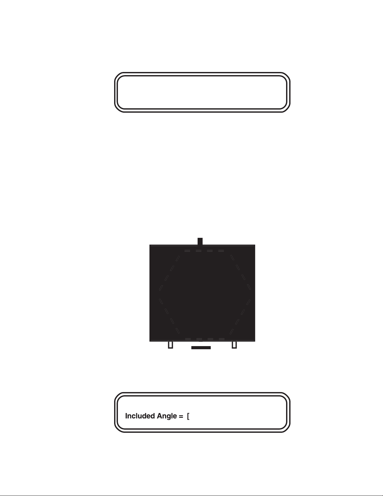
The two state mode allows the separation and resolution of almost all DNA size ranges.
The term two state refers to two field vectors. The directions of these two vectors are determined by the included angle. This angle is determined relative to the gel, as shown in Figure
4.1. In the two state mode the angle can be continuously varied between 0 and 180°. Linear
or nonlinear switch time ramps are also possible in this mode.
Flg. 4.1. Orientation of the included angle in the two state mode.
TWO STATE prompts the entry of voltage gradient, run time, included angle, and switch
time (ramp or no ramp). When TWO STATE is pushed, the following screen is displayed:
V/cm: Enter the voltage gradient using the number key pad, and press ENTER. The total
voltage applied across the electrodes is obtained by multiplying the gradient by 33.5
[
[
]
_
17
Ratio: # : # ______Volts Ramp a = _______
State 1State 2
➤
➤
Included
angle
Gradient =
]V/cm Run Time =
Page 22

(33.5 cm is the distance across the hexagonal electrode array). The allowable voltage gradient range is 0.6–9.0 V/cm in 0.1 V/cm increments.
Run Time: Enter the total run time for the two state run, and press ENTER. The allowable run
time range is 1 minute–999 hours. Enter the run time as one time unit, either hours or minutes.
When entering the run time, put in the numeric value, then press HOURS or MINUTES.
Note: If a mistake is made while keying in a value, press CLR ENTRY, and start again.
If the value has been entered before the mistake is found, make the correction using the
editing mode (see Section 4.9).
Included angle: Enter the included angle, and press ENTER. The angle entered must be in
degrees, between 0 and 180. Caution: the efficacy of included angles < 90° has not been
proven.
After the data for the first screen are entered, the following screen will appear:
Int. Sw. Tm: To enter the initial switch time, enter the numeric value, press HOURS,
MINUTES, or SECONDS, then ENTER. The allowable switch time range is 0.05 seconds–18
hours. Enter the switch time as one time unit, e. g., enter 3 minutes and 30 seconds as 3.5
minutes or 210 seconds.
Fin. Sw. Tm: To enter the final switch time, enter the numeric value, press HOURS,
MINUTES, or SECONDS, then ENTER. The allowable switch time range is 0.05 seconds–18
hours. The values are entered as in the initial switch time. If the final switch time is the same
as the initial switch time, press ENTER.
Ramping factor: a =: The ramping factor display will appear only if there is a difference
between initial and final switch times. The value “a” is the ramping factor and determines
the mathematical shape of the ramp. For more information on the ramping factor, see Section
9.2. To run a linear ramp, press ENTER.
After all the values are entered for this screen, the CHEF Mapper system will display:
A Program is in memory. Please enter another command. The program that was just
entered is now in a short term memory (RAM). If the CHEF Mapper system is turned off, the
program will be lost. The following options are available:
Start Run: Press START RUN, and the run will begin. If power goes off during a run,
the program is saved and resumes when power is restored. When the run is completed,
only the AC power light will be on, and the screen will display: Run is Completed.
Press 1 to save, or 0 to clear it. To delete the program, enter 0. To save the program, enter
1. The program can be rerun until the power is turned off. To store the program, press
STORE PGM (see Section 4.8).
Edit the Program: To check the program just entered for errors or to make corrections,
see Section 4.9.
Store Program: To store the program just entered so that it is available for future use, see
Section 4.8.
Delay Start: To enter a time delay before the run is started, see Section 4.7.
[
[
]
]
18
Int.Sw.Tm =
] FinSw.Tm =
Page 23

Remove Program and set up a new Program: To delete the program just entered, press
either AUTO ALGORITHM, FIGE, TWO STATE, or MULTI STATE. The message
You will destroy last Program - Go On? will appear. Press 1 then ENTER to delete
the program. Enter 0 to save the program.
Running Two State
While a two state program is being run, the following screens are displayed:
Screen 1:
Run time: The total run time is shown in hours or minutes.
Remaining: The time remaining to the end of the run (i.e.: a countdown clock).
ma: The total electrode current in milliamperes.
Sw. tm: The present switch time. This will change during a ramp.
Angle: Present angle (half the included angle).
V/cm: The value of the voltage gradient.
Screen 2:
Included angle: This displays the included angle.
Volts: The actual voltage of the run (33.5 x gradient).
Ramp factor a: The ramping factor.
To move between the two screens during a run, use the ⇑ or ⇓ cursor keys.
4.5 The Multi State Mode
Entering Run Parameters into Multi State
The multi state mode allows flexibility in designing pulsed field regimens. Unlike the
two state mode, where the included angle between the two states determines the direction of
the field vector, multi state allows up to 15 independent vectors to be run in any combination.
Each vector (or state) has its own angle, voltage, and time of application (switch time). The
direction of each state is determined by its angle relative to a vertical line from the top to the
bottom of the gel, with the top being 180° and the bottom 0° (see Figure 4.2). Angles measured
counterclockwise from 0° are positive, and angles measured clockwise from 0° are negative.
s
r
__ma
19
Run Time = hh:mm Remaining = hh:mm
Included Angle = ____ ____volt
Ramping Facto
Page 24

Flg 4.2. Multi state angle example.
For example, to mimic a two state run, combine two vectors oriented at half the included angle on either side of the vertical (combinations of states are called blocks). This is
equivalent to a two state run with a 96° included angle.
A combination of states designed as a unit is called a block. There can be a total of eight blocks
per run, with each of these blocks composed of 1–15 states. Section 9.7 gives examples of
multi state runs.
When MULTI STATE is pushed, the following screen is displayed:
Intrp =: This prompt is asking if the program is to have interrupts (secondary pulses). Enter
0 if no interrupts are to be used and 1 if interrupts will be used. Interrupts are explained in
Section 9.3.
]
180°
20
0°0°+48°
-48°
96°
180°
180°
State 1
State 2
State 1 + State 2
-
+
➤
0°
Program with Interrupts? [
Page 25

Note: If no interrupts are chosen, interrupts cannot be used for any of the blocks 1–8. If
you don’t want interrupts for Block 1, but want interrupts for some later block, enter 1
(yes) for interrupts.
The first example shows how to enter run parameters in the multi state mode with no
interrupts. Next, an example for entering run parameters in multi state with interrupts is shown.
Blk1 Runtim: Enter the total run time for Block 1, and press ENTER. The acceptable run time
range is 1 minute–999 hours. Enter the run time as one time unit, either hours or minutes.
When entering the run time, put in the numeric value, then press HOURS or MINUTES.
Note: If a mistake is made while keying in a value, press CLR ENTRY, and start again.
If the value has been entered and then the mistake is found, make the correction using
the editing mode (see Section 4.9).
After the data for the first screen are entered, the following screen will appear:
V/cm: Enter the voltage gradient for Block 1, State 1 using the number key pad, and press
ENTER. The total voltage applied across the electrodes is obtained by multiplying the gradient
by 33.5 (33.5 cm is the distance across the hexagonal electrode array). The allowable voltage
gradient range is 0.6–9.0 V/cm in 0.1 V/cm increments.
Ang: Enter the angle, then press ENTER. The angle entered must be in degrees and in the
range from 0 to + or - 180°.
In Tm: Enter the numeric value for initial switch time for State 1, press HOURS, MINUTES,
or SECONDS, then ENTER. The allowable switch time range is 0.05 seconds–18 hours.
Enter the switch time as one time unit, e. g., enter 3 minutes and 30 seconds as 3.5 minutes
or 210 seconds.
Fn Tm: Enter the numeric value for the final switch time for State 1, press HOURS, MINUTES,
or SECONDS, then ENTER. The allowable switch time range is 0.05 seconds–18 hours. Enter
the values in the same way as the initial switch time. If the final switch time is the same as the
initial switch time, press ENTER.
a =: The value “a” is the ramping factor and determines the mathematical shape of the ramp.
The ramping factor is active only if there is a difference between initial and final switch times.
For information on the ramping factor, see Section 9.2. To run a linear ramp, press ENTER.
[
[
]
[
]
]
21
Blk1 Runtim - [ ] Intrp = [
Blk1 St01
Ang =
]V/cm a =
Page 26

After State 1 parameters are entered, the screen will ask if another State is needed.
Continue with another State?: To program another state, press 1, then ENTER. If another
state is not desired, press 0, then ENTER. To program a second state in the same block, enter
the appropriate values at the prompts.
Blk1 St02: You are now in Block 1, State 2. Continue with up to 15 states (vectors) for each
block. To program a different block, press 0 and ENTER when asked to Continue with
another State? The screen will appear as:
Continue with another Block?: To enter another block, press 1, then ENTER. Up to eight
blocks can be programmed. If another block is not desired, press 0, then ENTER. The system
will display the message: A Program is in memory. Please enter another command. At this
point the program can be initiated by pressing START RUN.
For example, second block prompts would appear:
Blk2 Runtim: Enter the total run time for Block 2, then ENTER. The allowable run time
range is 1 minute–999 hours. Enter the run time as one time unit, either hours or minutes.
When entering the run time, put in the numeric value, then press HOURS or MINUTES.
Note: The prompt for interrupts (Intrp) in Blocks 2–8 is active only if interrupts were
chosen for Block 1 (1= yes at Intrp prompt in Block 1).
[
[
]
[
]
[
] ]
[
[
[
]
22
Continue with another State (Vector) ?
Blk2 St02
Ang =
Continue with another Block?
Blk2 RunTim =
] Intrp =
Page 27

After the data for Block 2 run time are entered, the screen will appear for Block 2, State 1:
Blk2 St01: Enter values for voltage gradient (V/cm), angle (Ang), initial switch time (In Tm), final
switch time (Fn Tm), and ramping factor (a) in the same manner as Block 1, States 1 and 2.
After Block 2, State 1 parameters are entered, the screen will ask if another State is desired.
Continue with another State?: If another state is desired, press 1, then ENTER. If another
state is not desired, press 0, then ENTER.
For example, a second vector in Block 2 would be programmed from the following screen:
Blk2 St02: Enter values for voltage gradient (V/cm), angle (Ang), initial switch time (InTm),
final switch time (FnTm), and ramping factor (a) in the same manner as for Block 1, States
1 and 2.
After State 2 parameters are entered, the screen will ask if another state is desired. You
can enter up to 15 states per block.
Continue with another State?: If another state is needed, press 1, then ENTER. If another
state is not needed, press 0, then ENTER.
[
]
[ ]
[
]
[
[= [ ]
]
[ ]
[
]
[
[= [ ]
23
Blk2 St01
Ang =
Continue with another State (Vector) ?
Blk2 St02
Ang =
Vc/m a =
=
Vc/m a =
=
Continue with another State (Vector) ?
Page 28

If 0 is entered, the screen will request another block.
Continue with another Block?: For another block, press 1, then ENTER. If another block
is not desired, press 0, then ENTER. The system will display: A Program is in memory.
Please enter another command. The program that was just entered is in short term memory (RAM). If the CHEF Mapper system is turned off, the program will be lost. The following
program options are available:
Start Run: Press START RUN to begin. If power goes off during a run, the program is
saved and resumes when power is restored. When the run is completed, only the AC
power light will be on, and the screen will display the message Run is Completed. Press
1 to save, or 0 to clear it. To delete the program, press 0. To save the program, enter 1.
To store the program, press STORE PGM (Section 4.8).
Edit the Program: To check the program just entered for errors or to make corrections,
see Section 4.9.
Store Program: To store the program just entered so that it is available for future use, see
Section 4.8.
Delay Start: To enter a time delay before the run is started, see Section 4.7.
Remove Program and Set Up a New Program: To delete the program just entered,
press either AUTO ALGORITHM, FIGE, TWO STATE, or MULTI STATE. The mes-
sage You will destroy last Program - Go On? will appear. Choose 0 for no, 1 for yes,
or 2 to edit the program. Press 1, then ENTER, to delete the program. Entering 0 saves the
program.
When interrupts are desired, enter 1 at the opening screen.
The display will ask if the interrupts will be 180° from the vector (i.e., go in the opposite
direction the DNA is moving). If yes, enter 1. If you want to assign the angle of the interrupts, press 0 for no.
Blk1 Runtim: Enter the total run time for Block 1, and press ENTER. The acceptable run time
range is 1 minute–999 hours. Enter the run time as one time unit, either hours or minutes.
When entering the run time, put in the numeric value, then press HOURS or MINUTES.
]
]
24
ontinue with another Block ?
Program with Interrupts ?
Page 29

When interrupts have been requested, the Block 1 interrupt is programmed from the
following screen:
Blk1 Interrupt Parameters: These interrupt parameters can be used with any state in Block 1.
Note: If you don’t want interrupts for Block 1 but want to use them for other blocks, you
must enter values at this prompt. Put in 1 for each entry. When you enter the run param-
eters for each state in this block, enter 0 (no) when the prompt asks for interrupts.
V/cm: Enter the voltage gradient for the interrupt using the number key pad, and press
ENTER. The voltage gradient can be from 0.6 V/cm to the same values as the voltage gradient for the states used in the block. A value greater than that of the states can be entered, but
the actual value will not exceed that of the states.
Ang: Enter the angle for the interrupt vector, and press ENTER. The angle entered must be
in degrees, between 0 and + or - 180°. The display back will appear in the prompt if the interrupt angle of 180° from the vector was selected in the first screen.
Length: To enter the interrupt duration, enter the numeric value, push HOURS, MINUTES,
or SECONDS, then ENTER. The allowable switch time range is 0.05 seconds–59 minutes,
59 seconds.
Freq: This is the frequency of interrupts for a particular period. Enter the frequency by entering the numeric value, then ENTER. The next prompt is for the time unit. Press SECONDS,
MINUTES, or HOURS. The allowable ranges are 1–99 seconds, 1–99 minutes, 1–99 hours.
The time unit of the frequency cannot exceed that of the length. If such a value is chosen, the
system will not accept the value.
After the interrupt values are entered for a block, the screen will ask for the first vector
(State 1) of the block.
Blk1 St01: This indicates that you are in Block 1, State 1.
Intrp: If interrupts are to be run in this state, enter 1. If interrupts are not to be run in this
state, enter 0. Proceed as prompted to program all of the states and blocks.
[
[
]
m
/
]
25
]V/c
Angl
Length
Blk1 St01
]V/cm a =
Ang =
Page 30

Running Multi State
While a multi state program is being run, the following screens are displayed:
Screen 1
Blk: Block number.
St: State number.
V/cm: Voltage gradient of the present state.
Angle: Angle of the present vector.
I: Indicates the interrupt is on.
Blk time remaining: The time remaining to the end of the run (i.e.: a countdown clock).
ma: The current in milliamperes.
Screen 2
Blk: Block number.
St: State number.
Sw.tm: The present switch time. This will change during a ramp.
volts: The actual voltage of the run.
Run time: The total run time, shown in hours or minutes.
Screen 3
Blk: Block number.
St: State number.
Intrp: Indicates an interrupt for that state (0 = no, 1 = yes).
Ang.: The angle of the interrupt vector.
V/cm: The voltage gradient of the interrupt vector.
m
____
___St__ ___
s
_
____ma
26
Blk___St__ ___V/cm Angle = ____
Blk
w.Tm = hh:mm:s
Blk___St__ Intrp = __ Ang. = ___ ____V/c
Duration =
Page 31

Duration: The duration of the interrupt in seconds, minutes, or hours.
Freq: The frequency of the interrupt.
a =: The ramping factor.
To move between the three screens during a run, use the ⇑ or ⇓ cursor keys.
4.6 Clock Read and Delay Start
Clock Read
CLOCK READ can be used any time the CHEF Mapper system is on, even during a run.
Pressing CLOCK READ displays the current time as hours:minutes:seconds and the current
date as month/day/year. The hours are in 24-hour time, for example, 3:00 pm is shown as
15:00:00. The time and date will appear for 5 seconds each time the key is pressed.
To set the clock or date, press CLOCK READ and DELAY START simultaneously.
The display will be: Current time: hh:mm:ss
Enter new hours [ ]
After you enter the hour, the cursor will move to minutes, then seconds. Pressing ENTER
at any of these prompts without entering a new value retains the original value. Next, the cursor moves to month, day, and year.
Delay Start
DELAY START allows the system to be started at a preset time. To use delay start, enter
the run parameters of your program, then press DELAY START, which will prompt you to
enter the start time date. Enter the day, and press ENTER. For the same day, just press Enter.
After the date has been entered, the prompt will be for the hour in 24 hour time and then minutes. Enter the hour and minutes.
Note: Delay Start can be activated for up to 2 days, 23 hours, and 59 minutes from the cur-
rent time. If you enter a date that is more than 3 days in the future, the message Start
time more than 3 days away, Abort? will appear. Enter 0 for no to exit the Delay Start
mode. Enter 1 for yes to re-enter the delay parameters.
To activate Delay Start, press START RUN. The screen will display the message
A program is in memory. Please enter another command. At this point the delay start
instruction is in memory along with the run parameters of your program.
After delay start has been activated, the screen will indicate the current time and the
start time. Current Time: hh:mm:ss month/day/year
Start Time: hh:mm day
To exit the delay start mode after it has been activated, press ENTER. The message
Continue in the Delay until Start? will appear. Enter 0 (for no) to exit the delay start mode.
Enter 1 (for yes) to reactivate the delay start mode.
27
Page 32

4.7 Storage and Recall of Programs
Storage of Programs
Programs can be stored in a battery backed-up RAM, and will remain when the power to
the CHEF Mapper system is turned off. They can be removed only by using CLR MEM (clear
memory) or by reinitializing the CHEF Mapper system using the comma key. When
programs are stored, they can be recalled at any time. In practice, about 20 programs can be
stored. The total number of programs stored depends on the complexity of the programs
(i.e., how many blocks, states, or interrupts are used). If the programs are very simple, it is
possible to store up to 99 programs.
To store a program, first enter the run parameters, then press STORE PGM. The screen
display will be: Enter stored User Program Number: or Enter to abort. Enter the number
that the program will be stored under. If the program number is available, the screen will
display, The Program Number assigned is : ##. Make note of it for future use. Press
ENTER to continue. If the program number is not available, the screen will display Duplicate
User Program Number - Check and reenter, or enter new Program. Press Enter and the
next screen will list available program numbers. Press Enter again to return to the screen to
enter the stored program number.
Note: Program number 00 is reserved for temporary storage of the current program after
completion of the run.
If the CHEF Mapper system runs out of memory while trying to store a program, the
message Not enough memory to store program - Delete another program, and try again
is displayed. You can decide not to store the program, or go back and delete one or more programs in memory, then store the new program.
Recall a Program
To recall a program, press USER PROGRAM. The display will be: Enter stored User
Program number: [ ] or Enter to abort. Press ENTER to cancel the command or enter the
number of a stored program, then press ENTER. If you enter a number that does not correspond to a stored program, the display: User Program number not found - Check and
reenter, or enter a new Program will appear. A screen will appear listing the available
program numbers. Press ENTER to go back to the previous screen, then enter a new user
program number.
Clear User Program Memory
To clear a user program from memory, press CLR MEM. The display will be: Enter
stored User Program number: [ ] or Enter to abort. Press ENTER to cancel the command
or enter the number of a program, then press ENTER. After you enter a program number the
display This will delete User Program: ##. Delete? will appear. Enter 1 for yes or 0 for no.
CLR MEM deletes only one program at a time, not the entire memory. To clear the entire
program memory, hold down the comma key for six beeps. The display: Total Initialization
- All memory will be erased - Go on? will appear. Enter 1 for yes or 0 for no. Initialization
resets the CHEF Mapper system by erasing all memory, including the stored programs.
28
Page 33

4.8 Editing Parameters
The editing mode of the CHEF Mapper system lets you review or change any of the run
parameters before or during a run. To use the editing mode, first enter the run parameters into
the CHEF Mapper system using AUTO ALGORITHM, FIGE, TWO STATE, or MULTI
STATE. The screen will display A program is in memory. Please enter another command.
There are two methods for entering the edit mode before the run is started. Press FIGE, TWO
STATE, or MULTI STATE, depending on which of these modes was chosen for the run.
The screen will display You will destroy last program - Go on? Press 2 to edit, then press
ENTER. This will take you to the first prompt in the run program. The second way to edit a
program is to press BLOCK, RUN TIME, STATE, INITIAL and FINAL SWITCH INTERVAL, VOLTAGE GRADIENT, or ANGLE (see Figure 4.3). Pressing any of these keys will
call up the corresponding section of the run program.
Fig. 4.3. Editing keys on the CHEF Mapper system panel.
This section describes the editing keys and their functions. The keys cannot be pressed
while a program is in run mode.
FIGE Mode
Block: Pressing BLOCK positions the prompt at the forward voltage gradient. Since there is
only one block in FIGE, this key places the cursor at the first parameter in the block.
Run Time: Pressing RUN TIME positions the prompt at the run time.
State: Pressing STATE displays the message Do you want Forward or Reverse? Enter 0 for
forward, or 1 for reverse. The prompt is placed at the forward voltage gradient, the first parameter in the state.
Initial Switch Interval: Pressing INITIAL SWITCH INTERVAL positions the prompt at
either the forward initial switch interval or the reverse initial switch interval, depending on the
state being edited.
Note: If initial switch time is changed after the run is started, the new value will not be
displayed immediately. The current state must be completed before the new value becomes
active.
Final Switch Interval: Pressing FINAL SWITCH INTERVAL positions the prompt at either
the forward final switch interval or the reverse final switch interval, depending on the state
being edited.
Voltage Gradient: Pressing VOLTAGE GRADIENT positions the prompt at either the
forward voltage gradient or the reverse voltage gradient, depending on the state being edited.
Angle: Pressing ANGLE displays Do you want Forward or Reverse? Enter 0 for forward,
or 1 for reverse. The prompt is placed at the forward voltage gradient, the first parameter in
the state.
29
SWITCH INTERVAL
BLOCK
RUN
TIME
STATE
INITIAL FINAL
VOLTAGE
GRADIENT ANGLE
Page 34

Two State Mode
Block: Pressing BLOCK positions the prompt at the voltage gradient. Since there is only one
block in two state, this key places the cursor at the first parameter in the block.
Run Time: Pressing RUN TIME positions the prompt at the run time.
State: Pressing STATE positions the prompt at the voltage gradient, the first parameter in
the block.
Initial Switch Interval: Pressing INITIAL SWITCH INTERVAL positions the prompt at
the initial switch interval.
Note: If initial switch time is changed after the run is started, the new value will not be
displayed immediately. The current state must be completed before the new value becomes
active.
Final Switch Interval: Pressing FINAL SWITCH INTERVAL positions the prompt at the
final switch interval.
Voltage Gradient: Pressing VOLTAGE GRADIENT positions the prompt at the voltage
gradient.
Angle: Pressing ANGLE positions the prompt at the included angle.
Multi State Mode
Block: Pressing BLOCK displays the message Enter Block Number. Enter block number
1–8. The prompt will be placed at the run time parameter in the block number chosen.
Run Time: Pressing RUN TIME positions the prompt at the run time in the block being edited.
Entering the editing mode by pressing RUN TIME will place the prompt at the run time for
Block 1.
State: Pressing STATE will display the message Enter State Number. Enter state number
0–15 (State 0 is for interrupt information). The prompt is placed at the first parameter in the
state number chosen, which is the voltage gradient if there are no interrupts and the interrupt
prompt if there are interrupts.
Initial Switch Interval: Pressing INITIAL SWITCH INTERVAL positions the prompt at
the initial switch interval in the state being edited. If an interrupt screen is being edited, this
key places the prompt at the length of the interrupt parameter.
Note: If initial switch time is changed after the run is started, the new value will not be displayed
immediately. The current state must be completed before the new value becomes active.
Final Switch Interval: Pressing FINAL SWITCH INTERVAL positions the prompt at the
final switch interval in the state being edited. If an interrupt screen is being edited, this key
places the prompt at the length of the interrupt parameter.
Voltage Gradient: Pressing VOLTAGE GRADIENT positions the prompt at the voltage
gradient in the state being edited. If an interrupt screen is being edited, this key places the
prompt at the voltage gradient for the interrupt.
Angle: Pressing ANGLE positions the prompt at the angle in the state being edited. If an
interrupt screen is being edited, this key positions the prompt at the angle for the interrupt.
To edit an existing value, enter in the new value at the prompt, and press ENTER.
Note: If you enter a value that is not allowed, the original value will be kept. For exam-
ple, if you want to change the run time from 20 hours to 18 hours and you enter 18 without
entering hours, the previous entry, 20 hours, will be saved.
30
Page 35

It is not necessary to press CLR ENTRY before entering a new value. If you make a mistake while entering a new value, press CLR ENTRY, and make the correction. To move the
prompt from one parameter to another while in the edit mode, use ENTER or any of the four
cursor arrow keys. If you make mistakes entering values while in the edit mode, use the cursor arrow keys to go back to the mistake and correct it. When editing run times, interrupt
frequencies, interrupt length, initial switch times, and final switch times, enter the numeric
value first, then HOURS, MINUTES, or SECONDS. To leave the edit mode, use ENTER, the
down cursor arrow key, or the right cursor arrow key to move the prompt to the end of the program.
There are three methods for entering the edit mode during a run. Stop the run with STOP
RUN, press the comma key for 6 seconds during a run, or pause the run, then press the comma
key for 6 seconds. All of these methods will display the message You will destroy last
program - Go on?. Enter 2 for edit, then press ENTER. This will take you to the first prompt
in the program.
Note: Run time cannot be edited during a run. Run time can be edited only before the
run is started.
Section 5
The Auto Algorithm Mode
5.1 Operation
The auto algorithm is embedded in the microprocessor in the CHEF Mapper XA power
module. The auto algorithm calculates the optimal switch times, switch time ramp, field angle,
voltage gradient, and run time for the DNA molecules in your sample. The run conditions set
by the auto algorithm place the smallest DNA fragment specified approximately 9 cm from the
origin of an agarose gel. The fragments specified may be in your sample or a size standard.
To access the auto algorithm mode, press AUTO ALGORITHM . The following screen
will appear:
This screen is used to establish the size range of DNA to be separated.
Low: Enter the size of the smallest DNA fragment, press K-BASES or M-BASES, and
ENTER.
High: Enter the size of the largest DNA fragment, press K-BASES or M-BASES, and ENTER.
Note: The limits of the auto algorithm are from 1 kb to 6 mb. Any entries outside these
limits will not be accepted. If the number entered in high is greater than 6 mb, the screen
will display Auto Algorithm Error - Large DNA too big - Press ENTER. Press
ENTER to return to the screen displaying Please enter another command, and press
AUTO ALGORITHM to re-enter values within the limits of the algorithm. If the high
size is less than the low, the CHEF Mapper system will automatically reverse them.
When you press ENTER after entering the high DNA fragment, the screen will display
the following:
[
]
31
Molecular weight Low
] High
Page 36

Calibration Factor: Adjusts calculated run time by the fraction entered. Press ENTER for
default of 1.0 (NC = no change).
When you press ENTER after entering the calibration factor, the screen displays:
The auto algorithm will indicate the buffer type and concentration, buffer temperature, and
agarose type and concentration for the run. The auto algorithm requires that for DNA < 2.5
mb, 0.5x TBE at 14 °C, in a 1.0% PFC agarose gel be used. For DNA > 2.5 mb the buffer must
be 1.0x TAE at 14 °C, with a gel of 0.8% PFC agarose. Press ENTER. The screen display
indicates one of the following run conditions:
• For DNA between 1 kb and 50 kb, FIGE will be implemented. See Section 4.3.
• For DNA smaller than 2.5 mb, the two state operating mode will be implemented.
See Section 4.4.
• For DNA larger than 2.5 mb, the multi state operating mode will be implemented.
See Section 4.5.
You can change any of the auto algorithm parameters from the original screen or the edit
modes. To change any entry, move the cursor to the parameter you want to change using the
cursor arrows. Press CLR ENTRY, enter the value and dimension, and press ENTER. To
edit the run parameter screens during or after electrophoresis, see Section 4.9.
Pressing ENTER moves the cursor through the display screens to the final screen:
A program is in memory - Please enter another command. The CHEF Mapper system is
programmed and ready to start. After positioning the gel in the electrophoresis chamber and
closing the lid, press START RUN to begin electrophoresis.
5.2 Applications
The auto algorithm simplifies pulsed field electrophoresis. Optimized running conditions
are derived from extensive data stored in the CHEF Mapper system’s microprocessor and
implemented with a few key strokes. Sometimes, however, one or more fine-tuning modifications of the run parameters must be made to achieve a separation. For example:
• For DNA larger than 2 mb, run times can be hundreds of hours, because the auto algorithm
sets run conditions so that the smallest DNA to be separated will migrate approximately
9 cm from the origin. It is not always necessary to have the smallest DNA fragment,
particularly fragments over 2 mb, migrate the full 9 cm. Adequate resolution can often be
obtained when the smallest DNA moves only part of the way through the gel. Decreasing
the run time parameter will shorten the migration distances of the DNAs in the gel while
maintaining all other relevant parameter settings.
____
Molecular weight Low
]
[
]
32
Calibration Factor
Molecular Weight:
Low
Page 37

Note: Always edit the run time before pressing START RUN. After the run has started,
it is not possible to enter a new run time.
• Enter the low and high DNA size just outside the DNA size range to be optimized. For
example, to optimize the separation of DNA in the size range of 200 kb and 500 kb, enter
150 kb as the low DNA size and 550 kb as the high DNA size.
Important! When you are entering extremely wide size ranges in the auto algorithm (or its
counterpart in the interactive program disc), there is likely to be a band inversion in the mid
range of the gel. For example, a low size of 1 kb and a high of 6 mb results in a mobility
reversal somewhere in the 200–500 kb range.
Section 6
The Interactive Algorithm
6.1 Introduction
The PC based interactive algorithm allows greater flexibility in setting run conditions
than the auto algorithm in the CHEF Mapper system. It has two operating modes, fully
automated and semi-automated. The former exactly duplicates the auto algorithm embedded
in the CHEF Mapper system. It assumes standard 0.5x TBE, 1% PFC (low EEO) agarose,
and 14 °C. The interactive algorithm (semi-automated) allows you to vary the buffer type
and concentration, agarose type and concentration, and buffer temperature. As with the auto
algorithm, the lowest and highest fragment sizes are entered. The software then computes the
optimized operating parameters. Both of these algorithms are under the algorithm menu, with
a toggle to get from one mode to the other.
Both forms of the algorithm permit you to edit or change the calculated parameters before
electrophoresis, and to employ nonlinear switch-time ramps, although these are not used in the
calculations. The semi-automated mode also permits the use of interrupt pulses (see Section 9.3).
You may bypass either of these primary operating modes, and manually set up parameters in FIGE, two state, and multi state program menus. Nonlinear switch-time ramping is
permitted in all three modes, but interrupt pulses are allowed only in the multi state mode.
The results calculated by the fully automated and semi-automated programs will specify
FIGE, two state, or multi state, depending on the fragment range. The software automatically
selects the appropriate mode according to the following rules:
• If the largest fragment is < 50 kb, a FIGE routine will result. The smallest fragment will
be placed 9 cm from the well, or about 1 cm from the bottom of a standard gel.
• If the largest fragment is < 2,500 kb, a two state mode is selected. If the largest fragment
is < 2,500 kb and the smallest fragment is > 2,000 kb, either two state or multi state mode
is used.
• If the smallest fragment is < to 2,000 kb, and the largest fragment is > 2,500, multi state
(2 block) is used.
All routines are subject to an upper limit of 6,000 kb. When the smallest fragment is
> 2,000 kb, the separation time is such that high resolution occurs within 3 days, but the
fragment is not necessarily placed 9 cm from the well. The algorithms also have an effective
lower limit of 1 kb.
All data files may be saved on hard disk or floppy disk, or printed out.
All of the functions are easily accessed from the pull down menus across the top of the screen.
33
Page 38

6.2 Hardware and Software Requirements
The interactive program disc operates with Microsoft Windows 3.1 on IBM or compatible
computers of the AT class (80386) or faster. Generally, if a computer will operate with
Windows software, this program will run, but you should contact Bio-Rad before making a
specific computer purchase. The minimum RAM required is 512 K. A color monitor and
EGA or VGA graphics card are recommended. Monochrome systems operating with
Windows will generally give satisfactory displays.
6.3 Operation
This section assumes you are familiar with Microsoft Windows software. Consult the
Microsoft Windows manual for the basic techniques of using the mouse and dialog boxes.
Set-up
1. Insert the Algorithm start-up disc.
2. Open the Algorithm by double-clicking on the application or selecting it and choosing the
Open command from the file menu. The window displays the Menu Bar and control
points for programming, printing, and transmitting.
3. Choose Set-up from the File menu. The Default Program Mode window will appear.
Select Fully Automated or Semi-Automated Mode. The algorithm will default to whichever
mode is selected. It is not necessary to open this window except to change the default mode.
Algorithm
1. Choose Algorithm from the file menu. The CHEF Mapper Interactive Algorithm
dialog box will appear.
2. Select the Mode command. Toggle between Fully Automated and Semi Automated
Mode by clicking the Mode button. Fully Automated Mode allows entries of the
Minimum DNA Size and m Maximum DNA Size only, with other options inactive. The
Semi-Automated Mode allows choices of all options.
3. Select Semi-Automated Mode or Fully Automated Mode.
4. Enter the smallest size of DNA in kb in Minimum DNA Size either directly into the edit
field or with the slide bar.
5. Enter the largest size of DNA in kb in Maximum DNA Size either directly into the edit
field or with the slide bar. For Fully Automated Mode, continue with step 10.
6. Select the type of agarose by clicking the button next to the agarose type in Agarose Type.
34
Page 39

7. Select the concentration of the agarose by clicking the button next to the concentration in
Agarose Concentration.
8. Choose the buffer type and buffer concentration by clicking the button next to the buffer
type and concentration in Buffer Type.
9. Choose the temperature of the buffer by clicking the button next to the temperature in
Temperature.
10. Enter the ramping factor in the Ramping edit field. The allowable ramping factors are
shown in Figure 9.3. The factors for linear ramps are 0.00 or 100.00. The default ramp is
linear.
11. Enter a run time calibration factor in the Run Time Calibration field.
Note: You can adjust migration distances of the DNA bands by modifying the run time.
For example, agarose types other than those listed in the algorithm may affect the mobil-
ities of the DNAs. Run Time Calibration lets you compensate for conditions not
specified in the algorithm. Run Time Calibration factors are easily determined from
calibration gel runs. Prepare a gel with experimental reagents. Load samples of S. cere-
visiae standards. Use the Fully Automated Mode to determine the run conditions for
the size range of S. cerevisiae bands, 220 kb to 2,200 kb. Run the calibration gel and stain
it. Measure the distance from the well to the 220 kb band in cm. Divide this number into
9. The quotient is the Run Time Calibration factor. The default value of the run time
calibration factor is 1.0.
The algorithm run parameters have been entered. Click Calculate to calculate the
electrophoresis run parameters.
• For DNA between 1 kb and 50 kb, FIGE will be implemented, and the FIGE dialog box
will appear (See Program).
• For DNA smaller than 2,500 kb, the Two State operating mode will be implemented (See
Program).
• For DNA greater than 2,500 kb, the Multi State operating mode will be implemented
(See Program).
To save the program, click Save and enter a file name in the dialog box. To save only the
run parameter outputs, click Program Outputs. To save both the run parameter outputs and
the input parameters, click both the Program Outputs and Algorithm Inputs box. Click
OK to save. Click Cancel to return to the Program Outputs screen.
The program outputs may be edited by pressing Enter until the parameter to be edited is
highlighted. Enter the new value. Continue until all desired changes have been made. After
editing the Program Outputs, save and press OK.
Note: Always click OK after saving, editing, or viewing a Program Output or
Algorithm Input dialog box. Click Cancel only to return to the previous dialog box or
to enter new values.
Note: See Section 4.9 for editing programs in the CHEF Mapper system.
35
Page 40

Program
The CHEF Mapper algorithm allows run parameter entries into FIGE, two state, and multi
state modes. This section of the manual describes programming the CHEF Mapper system.
1. Choose Program from the file menu. Select FIGE from the Program menu. The
following screen will appear.
Enter the values for run time, forward and reverse switch times, voltage gradients, and
ramping factors in the appropriate edit fields.
Note: See Section 4.3 for the run parameter limits. Always enter values within the limits.
2. Select Two State from the Program file menu. The following screen will appear.
Enter the values for run time, initial and final switch time, voltage gradient, included
angle, and ramping factor.
Note: See Section 4.4 for the run parameter limits.
36
Page 41

3. Select Multi State from the Program menu. The following screen will appear.
The Multi State data screen allows entry of the number of blocks and states within blocks.
Enter the number of blocks in the Number of Blocks edit field. Enter the number of states per
block in the States For edit fields. Press OK to continue. Press Cancel to return to the file
menu screen.
Enter the values for the run time, initial and final switch time, voltage gradient, angle,
and ramping factor.
Note: See Section 4.5 for the run parameter limits.
Multi state mode allows an interrupt to be entered in each block of the program. To enter
an interrupt, click Enable Interrupt, and enter the duration, time between interrupts, voltage
gradient, and angle. To implement the interrupts in a state, press Activate Interrupt in each
state the interrupt is to be used. See Section 9.3 for interrupt parameters and strategies.
Print
To print the Algorithm Input and Program Output screens, use the Report file in the
Print menu.
37
Page 42

Section 7
Sample Preparation
7.1 Agarose Blocks and Liquid Samples
Standard procedures for DNA preparation do not yield intact, high molecular weight
DNA molecules. Large DNA molecules are so fragile that they are broken by mechanical
forces during their isolation. To prevent breakage of large DNA molecules, intact cells embedded
in agarose are lysed and deproteinized in situ. The agarose matrix protects the embedded
DNA from shear forces and provides an easy way to manipulate samples. Processed agaroseplug DNA inserts are loaded directly into sample wells of agarose electrophoresis gels.
Sample inserts are cast in Bio-Rad’s disposable sample mold, catalog number 170-3713.
Each sample mold produces fifty 10 x 5 x 1.5 mm agarose blocks. The block thickness allows
efficient diffusion of enzymes during sample preparation and permits samples to be loaded into
wells formed with Bio-Rad’s standard well-forming combs.
To prepare samples, mix intact cells at a predetermined concentration with molten Low
Melt Preparative Grade Agarose (catalog number 162-0017). Aliquot samples into the chambers of the mold and allow them to cool, then remove them from the mold and incubate with
detergents and enzymes to remove all of the cellular components from the DNA. After thorough washing, cut agarose plugs to appropriate size and place in the wells of the agarose gel.
A detailed procedure for preparation of Saccharomyces cerevisiae chromosomes is given in
Section 7.2.
High molecular weight DNA can be prepared by standard procedures. DNA fragments of
up to several hundred kilobases do not require preparation in agarose blocks, but can be added
to the wells in liquid form. When working with DNA in the range of 50–200 kb, it may be necessary to use pipet tips with large openings. When running only liquid samples, the best
resolution and sharpness of bands can be achieved by using a thin well comb (0.75 mm).
7.2 Procedure for
Saccharomyces cerevisiae
Chromosomal DNA
This procedure is modified from Schwartz and Cantor, 1986.
153
With some modification,
this procedure will work with most yeasts.
1. Grow yeast cells at 30 °C to stationary phase in YPD media (1% yeast extract, 2% dex-
trose, 2% bactopeptone) for 24–48 hours.
2. Pellet yeast cells by centrifugation for 10 minutes at 3,000 rpm.
3. Melt 1.6% low melt agarose in sterile water. Keep warm by placing in a 50 °C water
bath.
4. Wash the cell pellet twice with cold 50 mM EDTA, pH 8.0. Centrifuge for about 5 min-
utes at 1,600 rpm.
5. Discard supernatant and resuspend the cells with the equal volume of overnight culture
used.
6. Determine the concentration of yeast by counting a diluted sample on a hemocytometer
or by plating an aliquot on a YPD plate overnight at 30 °C. A final cell concentration of
7 x 10⁸cell/ml yields enough DNA for a run. Determine the volume of cells needed along
with the number plugs to make.
7. Pipet the volume of cells into another tube, add Lyticase [Sigma] (2 mg/ml in 0.01 M
sodium phosphate containing 50% glycerol) to a final concentration of 1 mg/ml.
38
Page 43

8. Add equal volume of 1.6% low melt agarose to the cell/enzyme suspension to give a final
agarose concentration of 0.8%.
9. Mix by inverting the tube several times. Keep the tube at 50 °C.
10. Using a disposable transfer pipet, pipet the sample into the plug molds. Allow the agarose
plugs to solidify at room temperature for about 30–45 minutes or plate at 4 °C for 20
minutes. Each well in Bio-Rad’s disposable plug mold holds approximately 100 µl of
sample.
11. Push the plugs out into a 50 ml Falcon tube containing ESP buffer (0.5 M EDTA, pH
9.0, 1 M Tris, pH 9.0, 10% N-Laurylsarcosine, 80 mg/ml Proteinase K. Take up desired
volume with 0.5 M EDTA, pH 9.0), using the provided snap-off tool on the plug mold.
12. Incubate the samples at 50 °C overnight (16–24 hours).
13. Aspirate off the ESP buffer and add enough volume to immerse the plugs with TE buffer,
pH 9.0. Let sit at room temperature for about 1 hour.
14. Decant the TE, pH 9.0 buffer and add fresh TE, pH 9.0 buffer. Let sit at room tempera-
ture for about 1 hour. Repeat wash two more times.
15. Store plugs in TE, pH 9.0 buffer at 4 °C for up to 1 year.
7.3 Procedure for Mammalian DNA*
An important application of pulsed field electrophoresis is the analysis of human and other
mammalian DNA. With this technique, fragments which are hundreds or thousands of kilobases
in length can be separated. Such fragments may contain entire gene families. Since mammalian
chromosomes are too large to enter gels with current technology, they must be digested with
restriction enzymes and visualized by probe hybridization. This section describes procedures
for preparing samples, restriction digestion, setting switch time parameters, and using appropriate controls. The DNA employed is from human white cells. Additional information on
sample preparation and pulsed field electrophoresis conditions is given in the references.
Sample Preparation
The following procedure will give a final concentration of 107cells/ml in the agarose.
Typical agarose slices contain 50–100 µl, giving 5–10 µg DNA per lane.
1. Harvest cells in phosphate-buffered saline:
A. Collect tissue culture cells by scraping or trypsination, followed by centrifugation.
Centrifuge suspension cultures directly, although brief trypsin digestion (0.25% in
saline) can improve lysis.
B. Prepare white blood cells from whole blood by either isotonic lysis or centrifugation
through Ficoll (e.g., Sigma Histopaque®). Starting volume is 5–50 ml blood.
C. Mince tissue with scissors or a razor blade and disperse to single cells with a loose
fitting Dounce homogenizer. Let large clumps of tissue settle, transfer supernatant,
and centrifuge.
2. Wash cells twice with PBS at 4 °C.
3. Count cells, and resuspend in PBS at a concentration of 2 x 10⁷cells/ml. Cells may be
counted in a hemocytometer (e.g., Reichert Inc.).
4. Gently pipet up and down to break up clumps, and warm to 37 °C.
39
Page 44

5. Mix with an equal volume of 1% low melting agarose prepared in PBS and cooled to
45 °C. Note: the agarose should be qualified for restriction digestion.
6. Transfer with a Pipetman® or disposable pipet to plug mold former, avoiding bubbles.
7. Allow samples to harden at 4 °C or on ice for 10 minutes.
8. Transfer sample blocks to 3–5 volumes of 0.5 M EDTA, pH 9, 1% Sarcosyl, 0.5 mg/ml
Proteinase K (Boehringer-Mannheim).
9. Digest for 1–2 days at 50 °C with constant, gentle shaking. Samples may be stored in
this solution at 4 °C.
*Contributed by Dr. Bruce Birren, California Institute of Technology
Restriction Digestion of DNA In Agarose
1. Rinse samples twice in distilled water. Wash with 50x volume of TE either twice for
3 hours at room temperature or overnight at 4 °C by gently shaking or rotating in 15 or
50 ml conical bottom polypropylene tubes.
2. Optional: Residual Proteinase K may be inactivated by washing sample in TE with 1
mM PMSF (phenyl methyl sulfonyl fluoride) twice for 2 hours at room temperature prior
to final washes in TE. Step 1 is usually sufficient.
3. Digest samples with a restriction enzyme in 100 µl to 200 µl final volume, depending on
the thickness of the plug. To the sample, add 10–20 µl 10x digestion buffer as recom-
mended by the supplier of enzyme, nuclease free BSA to 0.1 mg/ml, distilled water, and
enzyme.
4. Digest agarose blocks with 2–10 U enzyme per µg DNA. Incubate 4 hours to overnight
at the appropriate temperature. Enzymes may be added twice, once at the beginning and
again partway through the incubation. This is recommended for enzymes that have short
lifetimes. (Refer to the manufacturer’s specifications.)
5. Stop the reaction by adding 1 ml 0.5 M EDTA. Incubate 5 minutes at room temperature.
6. Remove EDTA from sample. Place agarose slices into the wells of an agarose gel. It is
important that the blocks are flat against the front wall of the well; remove any trapped
bubbles. Fill the void space with 0.8% low melting agarose. Alternatively, place blocks
on each tooth of the gel forming comb, and cast gel around the comb.
7. Place gel in chamber, and equilibrate at the running temperature for 0.5 hour prior to
starting the run.
Electrophoresis and Results
The use of pulsed field electrophoresis to identify large fragments of human DNA homologous to a cDNA probe is illustrated in Figure 7.1. Human DNA was digested with two
different rare cutting enzymes and separated for 36 hours before blotting and hybridization.
With Mlu I, three bands are visible between about 450 and 600 kb. Nru I yields two bands in
this size range, one at 450 and one at 670 kb. In addition, with Nru I there is a faint hybridization signal from the region near the top of the gel that contains unresolved large DNA. The
yeast markers indicate that the upper range of resolution of this gel is 900 kb. Thus, a hybridization signal in this upper region could indicate partial digestion products or the presence of
fragments above 2 mb. In the stained gel, Figure. 7.2A, only the largest S. cerevisiae
chromosomes are resolved, though the S. pombe chromosomes are well separated. When the
Nru I digest is run under the same conditions, the two bands which had been well resolved in
Figure. 7.1 are visible only as a smear. However, the two larger bands are distinguishable,
one at about 2 mb and the other at 2.5 mb. Not I yields a single large band at about 2.2 mb.
40
Page 45

The importance of using the appropriate switch interval when analyzing pulsed field data
is apparent from Figure 7.3. An Mlu I digest of human DNA was run using three different
pulsed field conditions prior to blotting and hybridization. Each of the gels resolved a different size range of DNAs, as indicated by the marker sizes in the figure. Under conditions where
only fragments from 200 to 600 kb were resolved, four bands were visible on the autoradiogram. When longer switch intervals were employed, so that fragments up to 1,600 kb are
separated, three bands are visible. In this experiment the central band appears darker than the
other two. Often, however, they are of uniform intensity and provide no clue to the doublet
lurking there. Using conditions which resolve bands above 2 mb, only a smear is seen on the
autoradiogram, in a position corresponding to the massed S. cerevisiae chromosomes. Thus, to
obtain accuracy in both sizing and in establishing the number of bands in Southern blots, gel
conditions that maximize resolution in the area containing the bands of interest must be used.
Numerous other factors can influence the ability to detect and accurately size bands of
interest in pulsed field gels. The most common reasons for failure include:
• The DNA samples are degraded by nuclease either during the sample preparation or dur-
ing the restriction digestion. Degradation during preparation produces plugs which yield
small DNA when run directly after preparation. Test each new batch of samples for con-
taminating nuclease by performing a mock digestion and running the products on a pulsed
field gel. The mock digestion consists of incubation at the same temperature and time in
a restriction digestion reaction minus the restriction enzyme (i.e., DNA+buffer+BSA).
Samples which are free of nuclease will have almost all the DNA remaining in the plug
or moving with the limiting mobility region of large unresolved DNA.
• Incorrect gel conditions are used. Size markers should indicate that the conditions used
(especially voltage and switch time) were appropriate for resolving the size region of
interest. Each new digest must be analyzed under a variety of gel conditions. Generally,
it is best to start with the conditions which give as broad a range of sizes as possible for
a rough estimate of the number and sizes of bands (this is often facilitated by using a
switch time ramp). Then gels which focus on a narrower size range can be used to more
precisely determine the sizes of the fragments.
• Incomplete restriction digestion can result from protein remaining in the samples or from
incomplete removal of the agents used to prepare the DNA (EDTA, protease, detergent).
In addition, because many of the enzymes used to generate large fragments are sensitive
to methylation, it can be extremely difficult to cut particular methylated sites. Using DNA
prepared from different sources (e.g., fibroblasts instead of blood) can often give differ-
ent length fragments due to tissue-specific methylation patterns.
• Sample overloading. The apparent size of fragments in pulsed field gels is strongly depen-
dent on the amount of DNA loaded in the gel. With increasing amounts of DNA, bands
are retarded in their migration, and indicated larger than true sizes. Figure 7.4 shows
hybridization to two different amounts of the same restriction digest run side by side.
Two distinct bands are visible in lane 1. As expected, an increased amount of DNA leads
to broadening of both bands. Furthermore, the midpoint of each of the broad bands is
shifted higher in the gel. This is particularly clear for the band near the bottom of the
autoradiogram. A lighter exposure of the pattern in lane 2 indicates a larger size for each
of the two bands than is seen in lane 1.
41
Page 46

Conclusion
In these experiments a cDNA probe was used to localize those large restriction fragments
bearing homology to the sequence of interest. Multiple bands were detected with each of the
enzymes used. Numerous situations can give rise to multiple bands on blots with large DNA.
These include the presence of multiple regions homologous to the probe (both genes and
pseudogenes), partial digestion due to restriction enzyme inhibitors in the samples or interference with cutting by methylation, or allelic differences between chromosomes that make
up the sample. Distinguishing between each of these cases requires knowledge of the factors
which influence pulsed field mobility and application of standard molecular biological methods to explain the nature of each of the bands.
Fig. 7.1. Separation and identification of fragments smaller than 1 megabase. A. Gel stained with
ethidium bromide. Human DNA in agarose blocks (5 µg/lane) was digested for 6 hr with 40 U of
enzyme in a reaction volume of 150 µl. Following digestion, samples were run in a 1% agarose gel, 6
V/cm for 36 hr in 0.5x TBE at 14 °C. Switch time was a ramp from 55 sec to 75 sec. Samples were:
Lane 1, Yeast size standard (YNN295). Lane 2, Mlu I digest. Lane 3, Nru I digest. Sizes (in kb) are indicated to the left of the yeast standards. B. Autoradiogram showing the position of bands identified by
the probe. After staining, the gel was exposed for 1 minute on a short wave UV light box (254 nm, 2
mW/cm). DNA was denatured in NaOH/NaCI, neutralized with Tris/NaCI and transferred overnight with
10x SSC to Zeta-Probe®membrane according to the manufacturer’s protocol. The hybridization probe
was a cDNA clone for a human G protein b subunit labeled by random priming.
42
AB
1 2 3 1 2 3
830-
690-
450-
215-
Page 47

Fig. 7.2. Separation and identification of fragments larger than 1 megabase. The samples in
Figure 7.1 were separated in 0.8% agarose for 108 hr in 1x TAE at 14 °C, 2 V/cm. Switch time was 35
min. A. Ethidium bromide stained gel.
S. cerevisiae
chromosomes are on the far left,
S. pombe
on the
right, with sizes indicated in megabases. Lane 1, Nru l; Lane 2, Not 1. B. Autoradiogram after
hybridization. Hybridization was as described in Figure 7.1.
Fig. 7.3. Importance of switch interval for resolving fragments. Human DNA was digested with Mlu
I for 6 hr and separated with different switch times or other pulsed field parameters. After membrane
separation, DNA was transferred to Zeta-Probe membrane as described in Figure 7.1. A. 1% gel electrophoresed for 36 hr at 6 V/cm with a switch ramp from 30 sec to 60 sec. B. 1% gel electrophoresed
36 hr at 6 V/cm with a ramp from 95 sec to 115 sec. C. 0.8% gel electrophoresed 108 hr at 2 V/cm
with a switch time of 35 min. Sizes indicate the position of the yeast markers included in each gel.
43
AB
1 2 1 2
2.2-
1.6-
1.1
-
-5.7
-4.7
-3.5
AB C
600-
550-
440-
215-
1125-
960-
836-
550460-
215-
5700-
4700-
3500-
22001125-
215-
Page 48

Fig. 7.4. Effects of sample overloading on hybridization signals. Human DNA was prepared in
agarose simultaneously using two different cell concentrations. A sample block of identical thickness
from each was digested with Not I and separated as described in Figure 7.3 The amounts of DNA
loaded per lane were: Lane 1, 3 µg. Lane 2, 15 µg. A. Ethidium bromide stained gel. B. Autoradio-
gram after hybridization. Blotting and hybridization were as described in Figure 7.1.
Section 8
Gel Electrophoresis
8.1 Casting the Gel
To cast the gel use a casting stand with removable end plates, platform, a comb, and a comb
holder. The casting stand which comes with the CHEF Mapper system is 14 cm (5.5”) wide x
13 cm (5”) long. Casting stands 21 cm (8.5”) wide x 14 cm (5.5”) long, or 14 cm (5.5”) wide x
21 cm (8.5”) long are available.
Cast the gel on a level surface. Bio-Rad’s Leveling Table (catalog number 170-4046) is
recommended for this purpose. For more detailed instructions, refer to the manual provided
with the casting stand.
1. Slide the platform into the casting stand. There is no sidedness to the platform. Position
one end gate over the screws protruding from the casting stand, insuring that the hori-
zontal slot is facing the platform. Slide the edge of the platform into the slot. Press down
on the end gate, and gently tighten the screws.
2. Position the other end gate over the screws, and slide it toward the platform until the edge
of the platform is inserted into the slot. Press down on the end gate, and gently tighten the
screws. The slots force the platform against the bottom of the casting stand.
3. To attach the comb to the comb holder, place the comb over the two metal pins, and turn
the screw clockwise. This causes one pin to move toward the screw, holding the comb in
place. Adjust the height of the comb to 2 mm above the surface of the platform by loos-
ening the screw (counterclockwise), then tightening when the comb is properly positioned.
A thin plastic ruler makes a good height gauge.
4. Place the comb holder (with attached comb) into one of the two positioning slots on each
side of the casting stand. Check that the bottom of the comb is at least 2 mm above the
surface of the platform. Prepare the desired concentration of Bio-Rad’s agarose in buffer.
Melt the agarose in a microwave oven or on a hot plate.
44
AB
1 2 1 2
Page 49

5. Carefully remove the comb holder and comb. It is sometimes helpful to rock the holder
back and forth slightly during removal. Sample plugs can be added to the wells while the
gel remains in the casting stand.
Compositions of Buffer Stock Concentrates
10x TBE Buffer: 108 g Tris base
(161-0733) 55 g boric acid
40 ml 0.5 M EDTA, pH 8.0
50x TAE Buffer: 242 g Tris base
(161 -0743) 57.1 ml glacial acetic acid
100 ml 0.5 M EDTA, pH 8.0
Fig. 8.1. The CHEF Mapper casting stand, comb holder, and disposable plug molds.
8.2 Buffer Circulation and Temperature
Level the CHEF Mapper electrophoresis chamber by adjusting the leveling screws. Place
the leveling bubble at the center of the chamber. Place the casting frame in the chamber. Pour
2.2 liters of buffer into the chamber. Switch on the CHEF Mapper power, then switch on the
variable speed pump. Circulate at ~1 L/min (a setting of ~70 on the pump regulator). Maintain
the flow rate at the maximum setting that does not disturb the gel. Allow the buffer to equilibrate to the desired temperature. We recommend 14 °C buffer temperature in chamber. The
temperature can be read by pressing ACTUAL TEMP on the Cooling Module panel. The
buffer can be chilled by the following methods:
• Attach the Cooling Module (see Cooling Module manual).
• Coil pump tubing into a temperature-controlled water bath with the temperature set so
that the buffer temperature in the gel chamber is 14 °C.
• Coil pump tubing into a bucket containing ice water, and measure the temperature in the gel
chamber. Continue to add ice or warm water to maintain the desired temperature during
the run.
45
Page 50

8.3 Sample Loading
Use one of the following methods to load the sample.
• Place DNA in a sample plug on a smooth clean surface and cut to size using a razor blade
or spatula. Samples should be less than 90% of the height of the wells. Place agarose plugs
onto the front walls of the sample wells using a spatula, and gently press them to the bottoms
of the wells. Press the plugs firmly against the front walls of the wells. Fill each sample
well with Low Melt Preparative Grade Agarose at an agarose concentration equal to that of
the gel, and allow the agarose to harden at room temperature for 10 to 15 minutes.
• Cut the sample plug into blocks and place on each tooth of the comb. Cast around the comb.
The plug will remain in place when the comb is removed.
• Add liquid samples to the sample wells with the gel positioned under the electrophoresis
buffer in the chamber. Turn the pump off when adding liquid samples to prevent samples from
washing out of the wells. Run the samples into the gel for approximately 5 to 10 minutes
before turning the pump back on.
8.4 DNA Size Standards
Run standards in each gel to verify the sizes of unknown samples and to verify the electrophoresis conditions. Figure 8.2 shows three of Bio-Rad’s standards for pulsed field
electrophoresis. These come as blocks of 0.75% low-melt agarose. Recommended run
conditions are given in the figure legend.
Fig. 8.2. Pulsed field standards, Lambda ladder (170-3635). Switch time was ramped from 50 seconds
to 90 second over the 22 hour run time. The gel was 1.0% agarose in 0.5x TBE. Electrophoresis was at
6 V/cm at 14 °C.
Schizosaccharomyces pombe
( 170-3633) Strain 972 h-. Switch time was 30 minutes
for 72 hours. The gel was 0.6% Chromosomal Grade Agarose in 0.5x TAE. Electrophoresis was at
1.5 V/cm at 14 °C.
Saccharomyces cerevisiae
(170-3605) Strain YNN295. Switch time was ramped from
60 seconds to 120 seconds over the 24 hour run time. The gel was 1.0% agarose in 0.5x TBE. Electrophoresis was at 6 V/cm at 14 °C.
8.5 Electrophoresis
Remove the end plates from both ends of the casting stand, and slide the gel on the black
platform into the black frame on the surface of the electrophoresis chamber under the buffer.
Place the gel in the chamber so that the platform is positioned inside the frame. Check the
buffer level to insure that the gel is covered by about 2 mm of buffer. Adjust the buffer flow
by using the flow adjustment knob on the Variable Speed Pump. Enter the run parameters
using either Manual with algorithm, Bar Code, or Memory Program Storage (see Section 4 for
complete instructions).
46
Lambda ladder
S. pombe S. cerevisiae
Page 51

Note: In prior models, do not insert additional gel stops at the upper comers of the gel. This
will affect the uniformity of the electric field and result in distortion of the outer lanes.
8.6 Separations at Room Temperature
Electrophoresis may be conducted at room temperature, without a chiller, but the buffer
should not be allowed to exceed 30 °C. It is important to maintain the temperature at a steady
value. To facilitate heat transfer, coil 4–5 feet of the Tygon tubing into a bucket of water.
Buffer recirculation is required. Change the buffer every 24 hours. Since heat generation is
proportional to the square of the voltage, it is essential to lower the field strength to 4.5 V/cm
or less, depending on the size of DNA to be resolved. Saccharomyces cerevisiae should be
electrophoresed at 3.8–4.5 V/cm. Gel strength and buffer concentration do not need to be
changed, although switch times and run times may be increased 10 to 20% at the lower field
strength. The conditions for resolution of Saccharomyces cerevisiae DNA are the same as
those given in Section 9.5, except that the voltage should be reduced to 4.5 V/cm when the
temperature is 29 °C.
Alternatively, the ionic strength of the buffer may be decreased to 0.25x TBE. In this
case, voltage must be decreased, or some DNA may not enter the gel. In some cases, DNA
bands may be more diffuse at room temperature than when resolved at 14 °C.
8.7 Removing and Staining the Gel
Before removing the gel, make sure the run is completed. To stain the gel during a run,
push PAUSE/CONT on the CHEF Mapper panel, and wait until the high voltage indicator
light goes off. Remove the gel from the gel chamber, place it into a 0.5 pg/ml ethidium bromide solution in water, and let the gel stain for 20–30 minutes. (Caution: ethidium bromide
is a mutagen. Always wear gloves while handling gels or solutions containing the dye.) Destain
the gel in distilled water for 1–3 hours. The DNA can be visualized by placing the gel on a UV
transilluminator (254–360 nm), catalog numbers 170-3737, 170-3738, and 170-3745. Remove
the buffer from the gel box by unclamping the drain tube and allowing the buffer to drain
into a 2.2 liter container with the pump turned off. Discard used buffer, and reclamp the drain
tube. Leave the lid of the gel chamber open on one end when not in use.
Note: In prior models, leaving electrophoresis buffer in the gel chamber with the lid
closed, when not in use, can warp the lid.
Section 9
Applications
9.1 Strategies for Electrophoretic Separations
Several parameters must be considered before performing an electrophoretic separation
of very high molecular weight DNA. The separations of large DNA molecules in agarose
gels are affected by agarose concentration, buffer concentration, buffer temperature, switch
times, voltage, pulse angle, and total electrophoresis run time
Agarose Concentration
The agarose concentration determines the size range of DNA molecules separated and
the sharpness, or tightness, of the bands. Agarose concentrations of 1% are useful in separating DNA molecules up to 3 mb in size. Agarose concentrations in the range of 1.2–1.5% are
typically used for improved band tightness; however, run times will increase proportionately. Gel concentrations below 1% (0.5–0.9%) are useful in separations of extremely high
molecular weight DNA, greater than 3 mb, although the bands are more diffuse.
47
Page 52

Several agarose types allow easy handling of low concentration gels. These agaroses, in
the concentration range of 0.5–0.8%, can be used to decrease the run time in separation of large
DNA (> 1 mb). An example of this type of agarose is Bio Rad’s Chromosomal Grade Agarose
(catalog number 162-0133).
Buffer Concentration and Temperature
In pulsed field electrophoresis, the mobility of the DNA is sensitive to changes in buffer
temperature. As the buffer temperature increases, the mobility of the DNA increases, but the
band sharpness and resolution decrease. Chill the buffer to 14 °C to maintain band sharpness
and to dissipate heat generated during prolonged runs. Buffer recirculation is required to prevent temperature gradients from occurring. High voltage runs (300 V) exceeding 1 day require
buffer changes after each 24 hour period, to prevent buffer degradation.
Standard tris borate (TBE) at a concentration of 0.5x is the most commonly used buffer
in pulsed field electrophoresis. Tris-acetate buffer (TAE) at a concentration of 1.0x can be
used in place of TBE. Other buffer concentrations used are in the range of 0.25x –1.0x. In
Figure 9.1 two different gels, one using 0.5x TBE and the other using 1.0x TAE, were run to
show the difference in mobility of DNA in the two buffers.
Fig. 9.1. Two gels, one in 0.5x TBE and the other in 1.0x TAE, were run to show the difference in
mobility of DNA in the two buffers.
S. cerevisiae
chromosomes were separated on a 1% gel with a
60 second pulse for 15 hours, followed by a 90 second pulse for 9 hours, at 6 V/cm. Notice the
increased migration of the DNA molecules in the TAE gel when compared with the TBE gel.
Switch Times
The migration rate of DNA molecules through an agarose gel depends on pulse time,
voltage (field strength), pulse angle, and run time. In pulsed field electrophoresis, DNA
molecules are subjected to alternating electric fields imposed for a period called the switch
time. Each time the field is switched, the DNA molecules must change direction or re-orient
in the gel matrix. Larger molecules take longer to re-orient and have less time to move during
each pulse, so they migrate slower than smaller molecules. Resolution will be optimal for
DNA molecules with re-orientation times comparable to the pulse time. So, as the DNA size
increases, the pulse time must be increased to resolve the molecules. Under some conditions,
larger molecules may run ahead of smaller ones (Lai, E., Personal Communication).
48
0.5x TBE 1.0x TAE
Page 53

Voltage (Field Strength)
DNA migration will increase with increases in voltage or field strength. However, greater
migration is accompanied by decreased band sharpness. In general, as the size of the DNA
molecules increases, the field strength should decrease. At high field strengths (6 V/cm) some
very large DNA (>3 mb) cannot be resolved on the gel and the field strength must be reduced.
Moreover, some large DNA molecules will not enter the gels at high field strengths. Therefore,
in selecting the field strength for an experiment, a compromise between run time and resolution has to be made.
Pulse Angle
The CHEF Mapper system allows separations to be carried out with electric field vectors
oriented in any direction in the plane of the gel (0–360°). With two field vectors, resolution
of DNA molecules up to l mb is independent of the angle between them, as long as the angle
is obtuse (Birren, Lai, Clark and Hood, Science, 241, 1203-1205, 1988). It has been shown that
decreasing the included angle from 120° to 94° increases the velocity of the DNA, with the
mobilities of large DNAs (>1 mb) affected to a greater degree by the change in angle than are
smaller DNAs (<1 mb). Figure 9.2 shows the effect of the included angle on the separation
of S. cerevisiae chromosomes. Decreasing the included angle will decrease the resolution of
smaller DNA by causing them to pile up on each other. This same effect on small DNA can
be seen with long switch times. Decrease the included angle (<120°) when separating DNA
molecules larger than 1 mb.
Fig. 9.2. Separation of
S. cerevisiae
using angles from 120° to 94°.
Electrophoresis Run Time
The electrophoresis run time is determined by the migration rates of the DNA molecules
under investigation. The migration rates, in turn, are affected by the switch time, field strength,
and pulse angle. As the migration rate of the DNA molecules decreases, the electrophoresis
run time must be increased to adequately resolve the DNA molecules of interest.
9.2 Ramping Factor
The CHEF Mapper system lets you program switch time ramps in a variety of mathematical
shapes. The manner in which switch times are ramped from initial to final values influences band
spacing. By appropriate choice of the ramping factor, DNA bands can be spread out or compressed
49
120° 105° 100° 96° 94°
Page 54

as desired. Switch time ramps follow the general equation: y = [x/(x+a)]*(a+1), with a<-1 or a>0.
The 27 allowable ramp shapes are shown in Figure 9.3. Each curve is uniquely defined by its ramping factor, a. Another useful value defined by these curves is the half height percent. The half height
percent is the percentage of run time required for the switch time to reach a value equal to the initial switch time plus 50% of the total ramp. Two representative ramps are shown in Figure 9.4.
Ramping factors and corresponding half height percents are indicated. The program generates 27
discrete ramp shapes. Choose a desired ramp shape from Figure 9.3, then determine the ramping factor, a, from the accompanying key. Half heights are shown in parentheses following the
corresponding a value. Enter the desired a value at the a= prompt, or press ENTER for linear ramps.
An example of linear and nonlinear ramping is shown in Figure 9.5. Lambda ladders
were separated with three different ramp shapes. The most linear band spacing was obtained
with the nonlinear ramp that had an a value of 0.357 and a 21% half height. Presumably, this
was because the switch time regimen utilized 79% of the run time ramping relatively slowly
through the longer switch time values. Conversely, the spacing between smaller DNA bands
was expanded at the expense of the larger ones when the ramping regimen emphasized shorter
switch times (a = -1.357, half height percent = 79%).
Fig. 9.3. The 27 allowable ramplng factors.
1.0
0.8
0.6
0.4
0.2
0.0
0.0
0.2
0.4
0.6
0.8
1.0
a=0.00189 (1%)
a=0.01536 (2%)
a=0.03644 (3%)
a=0.06623 6%)
a=0.10728 (9%)
a=0.16382 (12%)
a=0.24297 (16%)
a=0.35741 (21%)
a=0.53179 (26%)
a=0.82122 (31%)
a=1.37891 (37%)
a=2.84830 (43%)
a=16.16970 (49%)
Block Run Time
1.0
0.8
0.6
0.4
0.2
0.0
0.0
0.2
0.4
0.6
0.8
1.0
a=-1.00189 (99%)
a=-1.01536 (98%)
a=-1.03644 (97%)
a=-1.06623 (94%)
a=-1.10728 (92%)
a=-1.16382 (88%)
a=-1.24297 (84%)
a=-1.35741 (79%)
a=-1.53179 (74%)
a=-1.82122 (69%)
a=-2.37891 (63%)
a=-3.84830 (58%)
a=-17.16970 (52%)
Block Run Time
50
Page 55

Fig. 9.4. Two examples of half height percent.
1.0
0.8
0.6
0.4
0.2
0.0
0.0
0.2
0.4
0.6
0.8
1.0
a=-1.35741
a= -1.35741, Half Height = 79%
Block Run Time
Half height area
1.0
0.8
0.6
0.4
0.2
0.0
0.0
0.2
0.4
0.6
0.8
1.0
a=.35741
a= 0.35741, Half Height = 21%
Block Run Time
Half height area
51
Page 56

Fig. 9.5. Three gels were run to show the difference In linear and nonlinear ramping. The first was
a linear ramp with a half height of 50%, the second was a nonlinear ramp with a half height of 21%,
and the third was a nonlinear ramp with a half height of 79%. Lambda ladders were separated on a
1% gel with a 6.8 to 54.3 second ramp for 21 hours, at 6 V/cm, in 0.5x TBE chilled at 14 °C.
9.3 Multi State Interrupts
In the multi state mode, the CHEF Mapper system allows the use interrupts during the run.
Interrupts theoretically allow the DNA to disentangle from obstructions in the gel matrix to
reduce band broadening and help larger molecules adjust to sudden changes in the field conditions. Consequently, run times may decrease [Zhang, T., Smith, C. L. and Cantor, C. R.,
Nucleic Acids Res., 19, 1291 (1991)]. Interrupts, or secondary pulses, allow periodic voltage
spikes to occur at a specific angle, duration, and frequency. The interrupt function has the
constraint that the interrupt voltage cannot exceed that of the primary voltage. If the number
of interrupts per cycle is small, higher voltages on the interrupts may be achieved by bypassing this function. The interrupts are then programmed as ordinary vectors in multi state mode
(up to 15 vectors/cycle).
9.4 Pulsed Field Conditions by DNA Size
The table below shows suggested run parameters that can be used for the various DNA
size ranges listed.
DNA DNA DNA DNA
1–100 kb 0.1–2.0 mb 2–4 mb > 4 mb
% Agarose 1.0–1.2% 0.8–1.2% 0.6–1% 0.5–0.8%
Buffer 0.5x TBE 0.5x TBE 1.0x TAE 1.0x TAE
Temperature 14 °C 14 °C 14 °C 14 °C
Voltage 6–9 V/cm 4.5–6 V/cm 2–3 V/cm 1.5–2.5V/cm
Pulse parameters 0.05–10 sec 10–200 sec 200–1,800 sec 10–60 min
Run times 2–15 hr 15–30 hr 24–72 hr 72–144 hr
Angle 0° + 180°, 120° 120° 120°, 106° 106°
52
50% 21% 79%
0.5
0.4
0.3
0.2
0.1
0.0
0
100
200
300
400
500
600
700
a = 0 (50%)
a = 0.357 (21%)
a = -1.357 (79%)
Migration (cm/hr)
Page 57

9.5 Pulsed Field Conditions by Organism
The table below shows the run parameters for various types of DNA samples. Photos and bar
codes for these examples are given in Section 9.7. All are performed at 14 °C except where noted.
DNA Agarose Pulse time Run time
DNA size (kb) conc. (seconds) (hours) Voltage Angle Buffer
Restriction 0.2–23 1.2% 0.09 a3 9 V/cm 120° 0.5x TAE
fragments
5 kb ladder 5–75 1.0% 1–6
b
11 6 V/cm 120° 0.5x TBE
Lambda 50–1,000 1.0% 50–90 c22 6 V/cm 120° 0.5x TBE
Ladder
Saccharomyces 200–2,200 1.0% 60–120 d24 6 V/cm 120° 0.5x TBE
cerevisiae
Candida 1,000–4,000 0.8% 120
e
24 4.5 V/cm 120° 0.5x TBE
albicans 240 36
Schizo- 3,500–5,700 0.8%
f
1,200 72 1.5 V/cm 120° 0.5x TAE
saccharomyces 1,800
pombe
Dictyostelium 3,600–9,000 0.8% f2,000–7,000 h158 1.8 V/cm 120° TBE
i
discoideum 7,000–9,600 82 1.5 V/cm 120°
(a) 0.09 second single switch time for 3 hours.
(b) Ramped from 1 to 6 seconds over 11 hours.
(c) Ramped from 50 to 90 seconds over 22 hours.
(d) Ramped from 60 to 120 seconds over 24 hours.
(e) 120 second switch time for 24 hours followed by a 240 second switch time for 36 hours
(2 blocks).
(f) Chromosomal Grade Agarose
(g) Ramped from 20 minutes to 30 minute over 72 hours.
(h) Two blocks, with voltage change in second block. Run temperature 10 °C. Cox, et. al.,
Proc. Natl. Acad. Sci. USA, 87, 8247-8251 (1990).
(i) 27 mm Tris base, 27 mm boric acid, 0.75 mm EDTA, pH 8.5.
9.6 Blotting Megabase DNAs
†
Southern Blot Transfer
Pulsed field electrophoresis is a powerful technique for physical mapping of genes in
various organisms. To determine the chromosomal location of a gene in a micro-organism
or the size of the restriction fragment containing a gene in mammalian systems, large DNA
fragments separated by CHEF are transferred onto membranes and detected by Southern
hybridization analysis. The procedures described for Southern transfer of DNA from standard agarose gels onto membranes are applicable to large DNA fragments separated by CHEF,
with the addition of the gel pretreatment step listed below.
Gel Pretreatment
Since DNA fragments larger than 20 kb cannot be transferred efficiently, DNA fragments
separated by pulsed field gels must be cleaved before transfer onto membranes. DNA can be
cleaved by using either acid (depurination) or UV irradiation. The depurination reaction is
† Contributed by Dr. Eric Lai, University of North Carolina
53
Page 58

harder to control and is extremely sensitive to temperature. Exposure to short-wave UV light
is a reliable method for nicking DNA in pulsed field gels before transfer.
Procedure
The following procedure was developed for use with the GS Gene Linker®UV chamber.
For optimal results, this protocol must be followed exactly.
1. Stain the gel with 1.0 µg/ml ethidium bromide (EtBr) for exactly 30 minutes with constant
agitation. Use a fresh dilution of EtBr stock for each gel. Do not destain the gel prior to
nicking.
2. Immediately UV irradiate the gel, using the GS Gene Linker chamber, with 60 mJoules
of energy. The gel should be photographed using very short exposures (<1 second) to
minimize exposure to UV radiation. The gel can also be destained if desired. Transfer
the nicked DNA to nylon membrane using alkali or neutral conditions (see discussion).
3. Soak the gel in 0.4 N NaOH, 1.5 M NaCI for 15 minutes. Transfer the DNA onto Zeta-
Probe®GT nylon membrane (162-0196) using 2 liters of 0.4 N NaOH, 1.5 M NaCl as the
transfer solvent.
4. Set up the capillary transfer as follows, from bottom to top:
• Corning Pyrex glass dish (28 x 18 x 4 cm)
• Plexiglass or plastic box for support, about 3 cm high and small enough to fit in the
glass dish (e.g., Eppendorf yellow pipette tip rack)
• Glass plate (16 x 20 cm)
• Two sheets of blotting paper as a wick (18 x 30 cm, S&S, GB002)
• Agarose gel (top side down)
• Zeta-Probe GT membrane cut to the size of the gel and prewetted with distilled water
• Two sheets of blotting paper (18 x 15 cm; S&S, GB002)
• A stack of paper towels 10 cm high
5. Transfer the DNA 24–48 hours.
6. Carefully remove the paper towel and blotting papers. Remove the membrane with the gel,
lay them gel side up, and mark the location of the wells and the orientation marker on
the top of the gel. The position of the wells can be accurately marked on the membrane
with a fine point permanent marker pen, cutting through the bottoms of the wells.
7. Neutralize the membrane in 0.5 M Tris, pH 7.0 (neutralization buffer) for 5 minutes,
followed by rinsing briefly in 2x SSC. Transferred DNA can be visualized on the
membrane by placing the damp blot on a transilluminator.
8. Dry the membrane by blotting onto 3MM or other adsorbent paper and proceed with
hybridization. UV crosslinking of the DNA to the membrane is not recommended with
this alkaline transfer method.
Discussion
• The procedure is based on gels approximately 6 mm thick. If thicker gels are used, the
staining period may be prolonged to allow diffusion of EtBr into the middle of the gels.
DNA that is not stained with EtBr will not be nicked by the UV light and thus will not be
transferred from the gel.
54
Page 59

• If the output of the UV light source is not known and no UV meter is available, you can
titrate your UV light source as follows. Run a CHEF gel with eight lanes of S. cerevisiae
chromosomes as markers using a switch time that will provide resolution from 200–1,000
kb. Stain the gel with EtBr, and photograph with medium-wave 302 nm UV light and
fast film (Polaroid type 667) to minimize nicking of DNA. Note the exposure time of the
photo. Cut the gel into eight strips, each containing a lane of separated yeast chromosomes. UV irradiate the strips with a 254 nm light source for time intervals of 5, 10, 15,
30, 45, 60, 90, and 300 seconds. If a 254 nm light source is not available, 302 nm light can
be used, but exposure times have to be lengthened approximately five-fold. Alkaline
transfer the gel strips as described, and stain the gels after transfer. Take a photograph of
the gel strips using the same UV light source, film, and exposure time as before transfer,
and compare it with the photograph before transfer. Choose the time period that results in
80–90% transfer of DNA. Do not choose the time intervals with complete transfer because
most of the transferred DNA fragments will be too short for effective hybridization. If
less than 10 second short wave UV irradiation is required, you may need to use a 302 nm
light source for taking the picture of the gel and cutting away excess gel area. As a general rule, 10 seconds or less exposure time is needed with a new UV transilluminator.
The UV output will decrease with time, to as little as 30% of its initial rating after 7 years.
• Presoaking the gel in NaOH prior to transfer decreases background and increases transfer efficiency.
• Pulsed field gels can be blotted onto membranes using 20x SSC as the transfer buffer
solvent with standard alkaline denaturation followed by neutralization. Alkaline transfer
onto nylon membranes gives as good or better sensitivity as standard transfers onto nitrocellulose filters. The alkaline procedure is much simpler and faster. In addition, nylon
membranes can be reused many more times than nitrocellulose filters. Some blots may be
reused as many as 20 times.
• DNAs separated on the CHEF-DR II, CHEF DR III, or CHEF Mapper system can also
be vacuum transferred onto nylon membranes in 4 hours using a commercial vacuum
blotter, such as the Model 785 Vacuum Blotter (165-5000), and NaOH as buffer.
• The DNA is transferred from the back of the gel (the side opposite the wells) onto the
membrane because irregularities in the surface of the gel frequently occur during solidification of these high percentage gels (1%). These surface artifacts will interfere with the
transfer of the DNAs from the gel. Transfer from the other side of the gel insures smooth
surface contact between the gel and the membrane.
• It is essential to neutralize the membrane after transfer to prevent changing the pH of the
hybridization buffer during hybridization.
• It is not absolutely necessary to bake nylon membranes after alkaline transfer since the
DNA should be fixed onto the membrane by NaOH.
• To monitor the efficiency of the transfer, stain the gel in neutralization buffer for 30 minutes
with 1 µg/ml EtBr. Take a photograph of the post-transferred gel, and compare with the
original picture.
55
Page 60

Section 10
Maintenance of Equipment
10.1 Replacing Electrodes
Rinse the gel chamber after every run. Remove dirt and buildup with laboratory detergent
and a fine cloth. Do not to touch the electrodes.
If an electrode breaks or leaks at the O-ring, it may be replaced. Additional electrodes
are available from Bio-Rad Laboratories (see Section 13).
To replace an electrode:
1. Turn the gel chamber upside down, and remove the six screws.
2. Lift off the base plate.
3. Remove the hexagonal nut on the wire, remove the nut on the electrode to be replaced, and
push down firmly on the post to remove the old electrode.
4. Turn the box over, insert the new electrode, pack with self-leveling silicone sealant (available at most hardware stores), and replace the nut.
5. Replace the wire and base plate.
If one of the pins to the serial cable bends, use tweezers to carefully straighten it.
Replacement cables may be ordered from Bio-Rad.
10.2 Fuses
If the DC voltage to the electrodes exceeds 300 V, the 0.5 ampere FB fuse may blow.
The high-voltage indicator light on the power module will go off. Replace the fuse by unscrewing the cartridge at the front of the power module. Replace with 0.5 ampere FB (fast blow)
fuse. Make sure the power module is off when replacing a fuse.
If there is a power surge, the SB fuses may blow. The AC light on the power module will
go off. The fuses are at the rear of the power module, mounted inside the power entry module. Replace the fuses with 3.0 A SB if your local voltage is 120 V or 100 V, or with a 1.5 A
SB if 220 V or 240 V.
If the unit still does not operate, contact Bio-Rad Laboratories. Do not attempt to open and
repair the power module, or the warranty may be voided.
56
Page 61

Section 11
Troubleshooting Guide
Problem Solution
Equipment:
No power 1. Check fuses at back of power module
2. Check source of A/C power
3. Contact Bio-Rad Laboratories
No voltage across electrodes, 1 Check that lid is on
with AC power light lit on 2. Check that serial cable is fully inserted at
power module both ends
3. Check that coiled interlock cable is firmly
attached
4. Confirm that all leads are properly attached
5. Check HV fuse on front panel (0.5 A FB) and
replace if necessary
6. Check that a programmed voltage gradient is not
set at 0
7. Check that unit is not set in pause mode
Gel floats away 1. Pump flow rate is too high or too low. Adjust
with Variable Speed Pump
No or low buffer flow 1. Look for kink in tubing
2. Check Cooling Module; buffer in the heat
exchanger can freeze if the chiller is cooling, but
the pump is not on
Gel band patterns appear very 1. Foreign object in chamber; remove
distorted; lanes very curved,* thermometer, gel stops at top of gel, etc.
bands sharp, but slanting 2. Insufficient or non-uniform cooling due to low
pump flow
3. Check that buffer is level with surface of gel;
use leveling feet
4. Check that field vectors add up to a net forward
migration
5. Replace damaged electrode
6. Buffer volume should be 2.2 L for models
purchased after 1994.
7. Power module fault; contact Bio-Rad
Laboratories
*Slight distortion of the outermost lane is normal
57
Page 62

Problem Solution
Applications:
Bands smeary or fuzzy 1. Excessive heating. Lower the voltage or ionic
strength of the buffer
2. Improper switch interval (see Section 9.1)
3. Gel percentage too low; increase
4. Sample degraded; impure enzymes, or wash
cycles too short (agarose blocks)
5. Agarose impurities; consult Bio-Rad
6. Sample overload; adjust sample concentration
Large DNAs not resolved 1. Lower the voltage gradient to below 2 V/cm
2. Increase switch time
3. Agarose impurities
High background in lanes 1. Insufficient washing of samples
2. Sample may be contaminated with RNA or
other material
3. DNA concentration too high
Distorted bands 1. Sample contains too high salt or detergent
concentration
2. Buffer breakdown; change every 24 hours
3. Wells were distorted; recast gel
4. Sample plugs were crushed when placed in
wells
5. Pump flow rate too low; check for kink along
tubing
Thick bands 1. Use thinner wells
2. Load less sample
58
Page 63

Section 12
References
12.1 Applications in Pulsed Field Electrophoresis
The following are references in pulsed field electrophoresis, primarily from 1987-1989.
The list surveys a wide area of applications and organisms, but is not exhaustive. Underlined
references use the CHEF-DR II pulsed field electrophoresis system.
Organism Reference numbers
Aspergillus 20
Bacteria 8, 49, 55, 80, 90, 93, 120, 128, 149, 152, 190, 195
Candida albicans 92, 110, 111, 112, 150, 170
Caulobacter 52
Dictyostelium 36
Drosophila 64, 204
Epstein-Barr virus 75
Giardia 2
Histoplasma 176
Human 9, 14, 27, 33, 37, 43, 50, 60, 66, 67, 82, 83, 88, 102,
122, 132, 133, 136, 137, 142, 144, 147, 183, 186,
189, 202
Leischmania 61, 69, 103, 135, 156, 163
Mouse 18, 19, 29, 89, 97, 179, 207
Mycoplasma 6, 25, 114, 139
Neurospora 96, 130
Paramecium 68
Plants 72, 187
Plasmodium 10, 42, 86, 138, 161, 171
Pseudomonas 7
S. cerevisiae 3, 23, 31, 54, 87, 91, 123, 124, 151,162, 166, 182,
194, 205, 206
S. pombe 28, 53, 73, 75, 119, 169, 184
Tetrahymena 38
Trypanosoma 113, 192
Ureaplasma 34
Application Reference Numbers
Alkaline blotting
(Zeta-Probe membrane) 120 , 131
Blotting 1, 9, 26, 31, 66, 72, 120, 125, 130, 145, 202
CHEF 13, 20, 26, 28, 30, 31, 36, 37, 39, 42, 45, 56, 57,
58, 61, 85, 91, 93, 94, 96, 107, 121, 123, 136, 139,
143, 145, 151, 156, 162, 163, 168, 171, 173, 197,
198, 201, 202
Chromosome rearrangements 127, 141, 147, 166
Circular DNA 8, 75, 78, 79, 104, 118, 159, 160, 163, 164, 190,
207
Cosmid mapping 14, 46, 70, 98, 173, 193
Diagnostics (e.g., cancer) 148
DNA over 5 megabases 20, 72, 130, 197
59
Page 64

DNA under 200,000 bases 12, 34, 39
, 77, 93
Epstein-Barr virus 75
FIGE 7, 12, 14, 15, 17, 24, 25, 33, 47, 65, 68, 77, 146,
173, 182, 187
FIGE with S. pombe 184
Gene amplification 108, 135, 191
Mapping 1, 18, 59, 66, 87, 134, 140, 199
Minute chromosomes 26, 113
OFAGE 23, 52, 54, 79, 82, 87, 147
On-off pulsing 98, 181
PACE 11, 32, 98
PFGE 16, 50, 102, 137, 138, 140, 153, 155, 189, 184,
202
PFG in acrylamide 84
PHOGE 5
Preparative 45
Ramps 17, 107, 142
Restriction enzymes 105, 120
Review of PFGE 99
RFGE 3, 4, 9, 122, 123, 157, 159, 180
RFLP polymorphism 7, 14, 40, 43, 50, 65, 85, 102, 109, 150
Sample preparation - bacteria 58, 167, 172, 195
Sample preparation - cell lines 167
Sample preparation - general 145, 155, 167, 188
Sample preparation - tissues 106, 167
Sample preparation-YACs 45
Secondary structure analysis 30, 118, 128
Single strand DNA 181
Size standards 39, 74, 116, 200
Strain characterization 35, 69, 71, 121
TAFE 51, 62, 63, 132, 148, 179
Theory 15, 22, 44, 48, 76, 81, 100, 101, 117, 126, 129,
130, 158, 174, 175, 177, 178, 185, 196
Two-D PFG 10, 203
Virus 15, 145
Visualization of DNA 154, 168
( microscope)
Yeast artificial
chromosomes (YACs) 10, 16, 41, 45, 93, 94, 95, 107, 115, 144, 183, 198
12.2 Reference List for Pulsed Field Electrophoresis
1. Abel, K. J. and Gross, K. W., Nucl. Acids Res., 16, 2111-2126 (1988).
2. Adams, R. A., Nash, T. E. and Wellems, T. E., Nucl. Acids Res., 16, 4555-4565 (1988).
3. Albig, W. and Entian K-D., Gene, 73, 141-152 (1988).
4. Amler, L.C. and Schwab, M., Molec. and Cell Biol., 9, 4903-4913 (1989).
5. Bancroft I. and Wolk, C. P., Nucl. Acids Res., 16, 7405-7417 (1988).
6. Bautsch, W., Nucl. Acids Res., 16, 11461-11467 (1988).
7. Bautsch, W., Grothues, D. and Tummler, B., FEMS Microbiol. Let., 52, 255-258 (1988).
60
Page 65

8. Beverley, S., Anal. Biochem., 177, 110-114 (1989).
9. Bickmore, W. A., Maule, J. C., Van Heyningen, V. and Porteus, D. J., Somatic Cell Mol. Genet.,
15, 229-236 (1989).
10. Biggs, B. A., Kemp, D. J. and Brown, G. V., Proc. Natl. Acad. Sci. USA, 86, 2428-2432 (1989).
11. Birren, B. W., Hood, L. and Lai, E., Electrophoresis, 10, 302-309 (1989).
12. Birren, B. W., Lai, E., Hood, L. and Simon, M.I., Anal. Biochem., 177, 282-286 (1989).
13. Blocher, D., Einspenner, M. and Zajackowski, J., Int. J. Radiat. Biol., 56, 437-448 (1989).
14. Blonden, L. A., Dunnen, J. T., van Paasen, H. M., Wapenaar, M. C., Grootscholten, P. M., Ginjaar,
H. B., Bakker, E., Pearson, P. L. and van Ommen, G. J., Nucl. Acids Res., 17, 5611-5621 (1989).
15. Bostock, C. J., Nucl. Acids Res., 16, 4239-4252 (1988).
16. Bowcock, A. M., Herbert, J. M., Wijsman, E., Gadi, I., Cavalli-Sforza, L. L. and Boyd, C. D.,
Proc. Natl. Acad. Sci. USA, 85, 2701-2705 (1988).
17. Bray, P. F., Barsh, G., Rosa, J-P., Luo, X. Y., Magenis, E. and Shuman, M. A., Proc. Natl. Acad.
Sci. USA, 85, 8683-8687 (1988).
18. Brockdorf, N., Amar, L. C. and Brown, S. D., Nucl. Acids Res. 17, 1315-1326 (1989).
19. Brody, H. and Carbon, C., Proc. Natl. Acad. Sci. USA, 86, 6260-6263 (1989).
20. Brown, W. R. and Bird, A. P., Nature, 322, 477-481 (1986).
21. Burke, D. T., Carle, G. F. and Olson, M. V., Science, 236, 806-812 (1987).
22. Cantor, C. R., Gaal, A. and Smith, C. L., Biochemistry, 27, 9216-9221 (1988).
23. Carle, G. F. and Olson, M. V., Nucleic Acids Res., 12, 5647-5664 (1984).
24. Carle, G. F. and Olson, M. V., Science, 232, 65-68 (1986).
25. Chen, T. L. and Manuelidis, L., Genomics, 4, 430-433 (1989).
26. Chen, X. and Finch, L. R., J. Bacteriol., 171, 2876-2878 (1989).
27. Cheng, J-F., Smith, C. L. and Cantor, C. R., Nucl. Acids Res., 17, 6109-6127 (1989).
28. Chikashige, Y., Kinoshita, N., Nakaseko, Y., Matsumoto, T., Murakami, S., Niwa, O. and
Yanagida, M., Cell, 57, 739-752 (1989).
29. Chou, H. S., Nelson, C. A., Godambe, S. A., Chaplin, D. D. and Loh, D. Y., Science, 238, 545-
547 (1987).
30. Chu, G., Electrophoresis, 10, 290-295 (1989).
31. Chu, G., Vollrath, D. and Davis, R., Science, 234, 1582-1585 (1986).
32. Clark, S. M., Lai, E., Birren, B. W., Hood, L. and Simon, M. I., Science, 241, 1203-1205 (1988).
33. Clevers, H. C., Dunlap, S., Wileman, T. E. and Terhorst, C., Proc. Natl. Acad. Sci. USA, 85,
8156-8160 (1988).
34. Cocks, B.G., Pyle, L.E. and Finch, L.R., Nucl. Acids. Res. 17, 6713-6719 (1989).
35. Coetzee, D. J., Kock, J. L. and Pretorius, G. H., J. Microbiol. Methods, 7, 219-225 (1987).
36. Cole, R. A. and Williams, K. L., Nucl. Acids Res., 16, 4891-4902 (1988).
37. Compton, D. A., Weil, M. M., Jones, C., Riccardi, V. M., Strong, L. C. and Saunders, G. F., Cell,
55, 827-836 (1988).
38. Conover, R. K. and Brunk, C. F., Molec. and Cell. Biol., 6, 900-905 (1986).
39
. Cooney, C. A., Galbraith, J. L. and Bradbury, M. E., Nucl. Acids Res., 17, 5412 (1989).
61
Page 66

40. Corcoran, L., Forsyth, K., Bianco, A., Brown, G. and Kemp, D., Cell, 44, 87-95 (1986).
41. Coulson, A., Waterson, R., Kiff, J., Sulston, J. and Kohara, Y., Nature, 335, 184-186 (1988).
42. Cowman, A. F., Morry, M. J., Biggs, B. A., Cross, G. A. and Foote, S. J., Proc. Natl. Acad. Sci.
USA, 85, 9109-9113 (1988).
43. Craig, J., Fowler, S., Skinner, J. D., Burgoyne, L.A. and McInnes, J. L., Applied and Theor.
Electro., 1, 23-28 (1988).
44. Crater, G. D., Gregg, M. C. and Holzworth, G., Electrophoresis, 10, 310-314 (1989).
45. Cuoto, L. B., Spangler, E. A. and Rubin, E. M., Nucl. Acids Res., 17, 8010 (1989).
46. Deaven, L. L., Hildebrand, C. E., Longmire, J. L. and Moyzis, R. K., Abstract # 77: Human
Genome I Conference, San Diego (1989).
47. Denko, N., Giaccia, A., Peters, B. and Stamato, T. D., Anal. Biochem., 178, 172-176 (1989).
48. Deutsch, J. M., Science, 240, 922-924 (1988).
49. Dingwall, A. and Shapiro, L., Proc. Natl. Acad. Sci. USA, 86,119-123 (1989).
50. Dunham, I., Sargent, C. A., Trowsdale, J. and Cambell, R. D., Proc. Natl. Acad. Sci. USA, 84,
7237-7241 (1987).
51. Edman, J. C., Edman, U., Cao, M., Lundgren, B., Kovacs, J. A. and Santi, D. V., Proc. Natl.
Acad. Sci. USA, 86, 8625-8629 (1989).
52. Ely, B. and Gerardot, C. J., Gene, 68, 323-333 (1988).
53. Fan, J-B., Chikashige, Y., Smith, C. L., Niwa, O., Yanagida, M. and Cantor, C. R., Nucl. Acids
Res., 17, 2801-2818 (1988).
54. Fasullo, M. and Davis, R. W., Molec. and Cell. Biol., 8, 4370-4380 (1988).
55. Ferdows, M. S. and Barbour, A. G., Proc. Natl. Acad. Sci. USA, 86, 5969-5973 (1989).
56. Ferris, S., Freeby, S., Zoller, P., Ragsdale, C. and Stevens, A., Amer. Biotech. Lab., 7, 36-42
(1989).
57
. Ferris, S., Sparrow, L. and Stevens, A., Australian J. Biotechnol., 3, 33-35 (1989).
58. Flanagan, J. L., Ventra, L. and Weiss, A. S., Nucl. Acids Res., 17, 814 (1989).
59. Fountain, J. W., Wallace, M. R., Bruce, M. A., Seizinger, B. R., Menon, A. G., Gusella, J. F.,
Michels, V. V., Schmidt, M. A., Dewald, G. W. and Collins, F. S., Science, 244, 1085-1087
(1989).
60. Fulton, T. R., Bowcock, A. M., Smith, D. R., Daneshvar, L., Green, P., Cavalli-Sforza, L. L. and
Donis-Keller, H., Nucl. Acids Res., 17, 271-284 (1989).
61. Galindo, O., Mons, B. and Van Der Berg, F. M., Exp. Parasitol., 34, 245-252 (1989).
62. Gardiner, K., Laas, W. and Patterson, D., Somat. Cell and Molec. Gen., 12, 185-195 (1986).
63. Gardiner, K. and Patterson, D., Electrophoresis, 10, 296-301 (1989).
64. Garza, D., Ajioka, J. W., Burke, D. T. and Hartl, D. L., Science, 246, 641-646 (1989).
65. Gejman, P.V., Sitaram, N., Hsieh, W-T., Gelernter, J. and Gershon, E. S., Applied and Theoret.
Electrophor., 1, 29-34 (1988).
66. Gemmill, R. M., Coyle-Morris, J. F., McPeek, F. D., Ware-Uribe, L. F. and Hecht, F., Gene Anal.
Techn., 4, 119-131 (1987).
67. Gessler, M., Simola, K.O. and Bruns, G. A., Science, 244, 1575-1577 (1989).
62
Page 67

68. Gilley, D., Preer, J. R., Aufderheide, K. J. and Polisky, B., Molec. and Cell. Biol., 8, 4765-4772
(1988).
69. Gomez-Eichelmann, M. C., Holz, G., Beach, D., Simpson, A. M. and Simpson, L., Molec. and
Biochem. Parasitol., 27, 143-158 (1988).
70. Graham, M. Y., Otani, T., Boime, I., Olsen, M. V., Carle, G. F. and Chaplin, D., Nucl. Acids
Res., 15, 4437-4448 (1987).
71. Grothues, D. and Tummler, B., FEMS Microbiol. Let., 48, 419-422 (1987).
72. Guzman, P. and Ecker, J. R., Nucl. Acids Res., 16, 11091-11105 (1988).
73. Hahnenberger, K. M., Baum, M. P., Polizzi, C. M., Carbon, J. and Clarke, L., Proc. Natl. Acad.
Sci. USA, 86, 577-581 (1989).
74. Hanlon, D. J., Smardon, A. M. and Lane, M. J., Nucl. Acids Res., 17, 5413 (1989).
75. Harris, A. and Bentley, D. R., Nucl. Acids Res., 16, 4172 (1988).
76. Heller, C. and Pohl, F. M., Nucl. Acids Res., 17, 5989-6003 (1989).
77. Hennekes, H. and Kuhn, S., Anal. Biochem., 183, 80-83 (1989).
78. Hightower, R., Metge, D. W. and Santi, D. V., Nucl. Acids Res., 15, 8387-8398 (1987).
79. Hightower, R. and Santi, D.V., Electrophoresis, 10, 283-289 (1989).
80. Hockett, R. D., de Villartay, J-P., Pollock, K., Poplack, D. G., Cohen, D. I. and Korsmeyer, S. J.,
Proc. Natl. Acad. Sci. USA, 85, 9694-9698 (1988).
81. Hofman, M. D., Schalkwyk, L. C. and Doolittle, W. F., Nucl. Acids Res., 14, 6983-7000 (1986).
82. Holzwarth, G., McKee, C., Steiger, S. and Crater, G., Nucleic Acids Res., 15, 10031-10044
(1987).
83. Inoko, H. and Trowsdale, J., Nucl. Acids Res., 21, 8957-8963 (1987).
84. Ito, T. and Sakaki, Y., Nucl. Acids Res., 16, 9177-9184 (1988).
85. Jabs, E. W., Goble, C. A. and Cutting, G. R., Proc. Natl. Acad. Sci. USA, 86, 202-206 (1989).
86. Janse, C. J., Boorsma, E. G., Ramesar, J., Van Vianen, P., Van der Meer, R., Zenobi, P., Casaglia,
O., Mons, B. and Van der berg, F. M., Exp. Parasitol., 68, 274-282 (1989).
87. Kaback, D. B., Steensma, H. Y. and DeJonge, P., Proc. Natl. Acad. Sci. USA, 86, 3694-3698
(1989).
88. Kenrick, S., Patterson, M., Speer, A., Fischbeck, K. and Davies, K., Cell, 48, 351-375 (1987).
89. Kingsmore, S. F., Snoddy, J., Choubey, D., Lengyel, P. and Seldin, M. F., Immunogenetics, 30,
169-174 (1989).
90. Kohara, Y., Akiyma, K. and Isono, K., Cell, 50, 495-508 (1987).
91. Kolakowski, L. F., Schloesser, M. and Cooperman, B. S., Nucl. Acids Res., 16, 10441-10452
(1988).
92. Kurtz, M., Cortelyou, M., Miller, S., Lai, M. and Kirsch, D., Molec. and Cell Biol., 7, 209-217
(1987).
93. Kuspa, A., Vollrath, D., Cheng, Y. and Kaiser, D., Proc. Natl. Acad. Sci. USA, 86, 8917-8921
(1989).
94. Labella, T. and Schlessinger, D., Genomics, 5, 752-760 (1989).
95. Lai, E., Nucl. Acids Res., 17, 8008 (1989).
96
. Lai, E., Nucl. Acids Res., 18, in press (1990).
63
Page 68

97. Lai, E., Barth, R. K. and Hood, L., Proc. Natl. Acad. Sci. USA, 84, 3846-3850 (1987).
98. Lai, E., Birren, B. W., Clark, S. M. and Hood, L., Nucl. Acids Res., 16, 10376 (1988).
99. Lai, E., Birren, B. W., Clark, S. M., Simon, M. I. and Hood, L., BioTechniques, 7, 34-42 (1989).
100. Lalande, M., Noolandi, J., Turmel, C., Brousseau, R., Rousseau, J. and Slater, G. W., Nucl. Acids
Res., 16, 5427-5437 (1988).
101. Lalande, M., Noolandi, J., Turmel, C., Rousseau, J. and Slater, G. W., Proc. Natl. Acd. Sci. USA,
84, 8011-8015 (1987).
102. Ledbetter, D.H., Ledbetter, S., van Tuinen, P., Summers, K. M., Robinson, T. J., Nakamura, Y.,
Wolff, R., White, R., Barker, D. F., Wallace, M., Collins, F. S. and Dobyns, W. B., Proc. Natl.
Acad. Sci. USA, 86, 5136-5140 (1989).
103. Lee, M. G-S., Atkinson, B. L., Giannini, H. and Van der Ploeg, L. H., Nucl. Acids Res., 16, 9567-
9586 (1988).
104. Levene, S. and Zimm, B., Proc. Natl. Acad. Sci. USA, 84, 4054-4057 (1987).
105. Levine, J. D. and Cech, C. L., Biotechnology, 7, 1033-1036 (1989).
106. Lindsten, T., Lee, N. E. and Davis, M. M., Proc. Natl. Acad. Sci. USA, 84, 7639-7643 (1987).
107. Little, R. D., Porta, G., Carle, G. F., Schlessinger, D. and Urso, M., Proc. Natl. Acad. Sci., 86,
1598-1602 (1989).
108. Looney, J. E., Chi, M., Leu, T-H., Flintoff, W. F., Troutman, W. B. and Hamlin, J. L., Molec. and
Cell. Biol., 8, 5268-5279 (1988).
109. Maeda, N., McEvoy, S. M., Harris, H.F., Huisman, T. H. and Smithies, O., Proc. Natl. Acad.
Sci. USA, 83, 7359-7399 (1986).
110. Magee, B. B., Koltin, Y., Gorman, J. A. and Magee, P. T., Molec. and Cell. Biol., 8, 4721-4726
(1988).
111. Magee, B. B. and Magee, P. T., J. Gen. Microbiol., 133, 425-430 (1987).
112. Magee, P. T., Rikkerink, E. H. and Magee, B. B., Anal. Biochem., 175, 361-372 (1988).
113. Majiwa, P. A., Young, J. R., Hamers, R. and Mattyssens, G., Gene, 41, 183-192 (1986).
114. Maniloff, J., Nucl. Acids Res., 17, 1268 (1989).
115. Marchuk, D. and Collins, F. S., Nucl. Acids Res., 16, 7743 (1988).
116. Mathew, K. M., Hui, C-F., Smith, C. L. and Cantor, C. R., Biochemistry, 27, 9222-9226 (1988).
117. Mathew, M. K., Smith, C. L. and Cantor, C. R., Biochemistry, 27, 9204-9210 (1988).
118. Mathew, M. K., Smith, C. L. and Cantor, C. R., Biochemistry, 27, 9210-9216 (1988).
119. Matsumoto, T., Fukui, K., Niwa, O., Sugawara, N., Szostak, J. W. and Yanagida, M., Molec.
and Cell. Biol., 7, 4424-4430 (1987).
120. McClelland, M., Jones, R., Patel, Y. and Nelson, M., Nucl. Acids Res., 15, 5985-6005 (1987).
121. McCluskey, K. and Mills, D., J. Cell Biochem. Suppl., O, 13, Part E (1989).
122. Miles, J. S., Bickmore, W., Brook, J. D., McLaren, A. W., Meeham, R. and Wolf, C. R., Nucl.
Acids Res., 17, 2907-2917 (1989).
123. Monia, B. P., Haskell, K. M., Ecker, J. R., Ecker, D. J. and Crooke, S. T., Nucl. Acids Res., 17,
3611 (1989).
124. Mortimer, R. K. and Schild, D., Microbiol. Rev. 49, 181-213 (1985).
125. Muller, U., Stephan, D., Philippsen, P. and Steinmetz, M., EMBO Journal, 6, 369-373 (1987).
64
Page 69

126. Noolandi, J., Slater, G. W., Lim, H. A. and Viovy, J. L., Science, 243, 1456-1458 (1989).
127. O’Connell, P., Leach, R., Cawthon, R. M., Culver, M., Stevens, J., Viskochil, D., Fournier, R. K.,
Rich, D. C., Ledbetter, D. H. and White, R., Science, 244, 1085-1087 (1989).
128. Ohki, M. and Smith, C. L., Nucl. Acids Res., 17, 3479-3490 (1989).
129. Olschwang, S. and Thomas, G., Nucl. Acids Res., 17, 2363 (1989).
130. Orbach, M., Vollrath, D., Davis, R. and Yanofsky, C., Molec. and Cell Biol., 8, 1469-1473 (1988).
131. Patarapotikul, J. and Langsley, G., Nucl. Acids Res., 16, 4331-4340 (1988).
132. Patterson, D., Gardiner, K., Kao, F-ZT., Tanzi, R. and Watkins, P., Proc. Natl. Acad. Sci. USA,
85, 8266-8270 (1988).
133. Patterson, M., Schwartz, C., Bell, M., Sauer, S., Hofker, M., Trask, B., van den Engh, G. and
Davies, K. E., Genomics, 1, 297-306 (1987).
134. Peltz, G. A., Grundy, H. O., Lebo, R. V., Yssel, H., Barsch, G. S. and Moore, K. W., Proc. Natl.
Acad. Sci. USA, 86, 1013-1017 (1989).
135. Petrillo-Peixoto, M. L. and Beverley, S. M., Molec. and Cell Biol., 8, 5188-5199 (1988).
136. Pohl, T. M., Zimmer, M., MacDonald, M. E., Smith, B., Bucan, M., Poustka, A., Volinia, S.,
Zehetner, G., Wasmuth, J. J., Gusella, J., Lehrarch, H. and Frischauf, A.-M., Nucl. Acids Res., 16,
9185-9198 (1988).
137. Pologe, L. G. and Ravetch, J. V., Cell, 55, 869-874 (1988).
138. Pritchard, C. A., Goodfellow, P. J. and Goodfellow, P. N., Nature, 238, 273-275 (1987).
139. Pyle, L. E., Corcoran, L. N., Cocks, B. G., Bergemann, A. D., Whitley, J. C. and Finch, L. R., Nucl.
Acids Res., 16, 6015-6025 (1988).
140. Rappold, G. A. and Lehrach, H., Nucl. Acids Res., 16, 5361-5377 (1988).
141. Resnick, M. A., Skaanild, M. and Nilsson-Tillgren, T., Proc. Natl. Acad. Sci. USA, 86, 2276-
2280 (1989).
142. Richards, J. E., Gilliam, T. C., Cole, J. L., Drumm, M. L., Wasmuth, J. J., Gusella, J. F. and
Collins, F. S., Proc. Natl. Acad. Sci. USA, 85, 6437-6441 (1988).
143
. Richmond, T., Biotechnol. Lab. News, Feb. 14 (1989).
144. Riethman, H. C., Moyzis, R. K., Meyne, J., Burke, D. T. and Olson, M. V., Proc. Natl. Acad.
Sci. USA, 86, 6240-6244 (1989).
145. Rohozinski, J., Girton, L. E. and Van Etten, J. L., Virology, 168, 363-369 (1989).
146. Roy, G., Wallenburg, J. C. and Chartrand, P., Nucl. Acids Res., 16, 768 (1988).
147. Rubin, C. M., Carrino, J. J., Dickler, M. N., Leibowitz, D., Smith, S. D. and Westbrook, C. A.,
Proc. Natl. Acad Sci. USA, 85, 2795-2799 (1988).
148. Russo, G., Isobe, M., Gatti, R., Finan, J., Batuman, O., Huebner, K., Nowell, P. C. and Croce, C.
M., Proc. Natl. Acad. Sci. USA, 86, 602-606 (1989).
149. Sanz, J. L., Marin, I., Ramirez, L., Abad, J. P., Smith, C. L. and Amils, R., Nucl. Acids Res., 16,
7827-7832 (1988).
150. Scherer, S. and Stevens, D. A., Proc. Natl. Acad. Sci. USA, 85, 1452-1456 (1988).
151. Schmidt, M. C., Kao, C. C., Rui, P. and Berk, A. J., Proc. Natl. Acad. Sci. USA, 86, 7785-7789
(1989).
152. Schoenline, P. V., Gallman, L. M. and Ely, B., Gene, 70, 321-329 (1988).
153. Schwartz, D. C. and Cantor, C. R., Cell, 37, 67-75 (1986).
65
Page 70

154. Schwartz, D. C. and Koval, M., Nature, 338, 520-522 (1989).
155. Schwartz, D. C., Saffran, W., Welsh, J., Haas, R., Goldenberg, M. and Cantor, C. R., Cold Spring
Harb. Symp. Quant. Biol., 47, 189-195 (1983).
156. Searle, S., Campos, A. J., Coulson, M. R., Spithill, T. W. and Smith, D. F., Nucl. Acids Res., 17,
5081-5095 (1989).
157. Serwer, P., Electrophoresis, 8, 301-304, (1987).
158. Serwer, P., Applied and Theoret. Electrophor., 1, 19-22 (1988).
159. Serwer, P. and Hayes, S. J., Applied and Theoret. Electrophor., 1, 95-98 (1989).
160. Serwer, P. and Hayes, S. J., Biochemistry, 28, 5827-5832 (1989).
161. Sheppard, M., Thompson, J. K., Anders, R. F., Kemp, D. J. and Lew, A. M., Mol. Biochem.
Parasitol., 34, 45-52 (1989).
162. Shih, C-K., Wagner, R., Feinstein, S., Kanik-Ennulat, C. and Neff, N., Molec. and Cell. Biol., 8,
3094-3103 (1988).
163. Simpson, A. M., Suyama, Y., Dewes, H., Campbell, D. A. and Simpson, L., Nucl. Acids Res., 17,
5427-5445 (1989).
164. Simske, J. S. and Scherer, S., Nucl. Acids Res., 17, 4359-4365 (1989).
165. Slater, G. W. and Noolandi, J., Electrophoresis, 10, 413-428 (1989).
166. Smith, C. L., Econome, J. G., Schutt, A., Klco, S. and Cantor, C. R., Science, 236, 1448-1453
(1987).
167. Smith, C. L., Klco, S. R. and Cantor, C. R., In Genome Analysis: A Practical Approach, Davies,
K. E., ed., IRL Press, pp. 41-72 (1988).
168. Smith, C. L., Matsumoto, T., Niwa, O., Klco, S., Fan, J., Yanagida, M. and Cantor, C., Nucl.
Acids Res., 15, 4481-4489 (1987).
169. Smith, S. B., Aldridge, P. K. and Callis, J. B., Science, 243, 203-243 (1989).
170. Snell, R. G. and Wilkins, R. J., Nucl. Acids Res., 14, 4401-4406 (1986).
171. Snewin, V. A., England, S. M., Sims, F. G. and Hyde, J. E., Gene, 76, 41-52 (1989).
172. Sobral, B. W. and Atherly, A. G., BioTechniques, 7, 938 (1989).
173. Sobral, B. W. and Atherly, A. G., Nucl. Acids Res., 17, 7359-7370 (1989).
174. Sor, F., Nucl. Acids Res., 16, 4853 - 4863 (1988).
175. Southern, E. M., Anand, R., Brown, W. R. and Fletcher, D.S., Nucl. Acids Res., 15, 5925-5943
(1987).
176. Steel, P. E., Carle, G. F., Kobayashi, G. S. and Medoff, G., Molec. and Cell Biol., 9, 983-987
(1989).
177. Stellwagen, J. and Stellwagen, N. C., Nucl. Acids Res., 17, 1537-1548 (1989).
178. Stellwagen, N. C. and Stellwagen, J., Electrophoresis, 10, 332-344 (1989).
179. Storb, U., Haasch, D., Arp, B., Sanchez, P., Cazenave, P-A. and Miller, J., Molec. and Cell Biol.,
9, 711-718 (1989).
180. Sutherland, J. C., Emrick, A. B. and Trunk, J., Electrophoresis, 10, 315-317 (1989).
181. Sutherland, J. C., Monteleone, D. C., Mugavero, J. H. and Trunk, J., Analyt. Biochem., 162, 511-
520 (1987).
182. Thiele, D. J., Molec. and Cell. Biol., 8, 2745-2752 (1988).
66
Page 71

183. Traver, C. N., Klapholz, S., Hyman, R.W. and Davis, R. W., Proc. Natl. Acad. Sci. USA, 86,
5898-5902 (1989).
184. Turmel, C. and Lalande, M., Nucl. Acids Res., 16, 4727 (1988).
185. Upcraft, J. A., Boreham, P. F. and Upcraft, P., Nucl. Acids Res., 17, 3315 (1989).
186. US Congress, Office of Technology Assessment, Mapping our Genes- the genome projects, how
big, how fast? OTA-BA-3, Washington, DC. US Government Printing Office (1988).
187. Van Daelen, R. A., Jonkers, J. J. and Zabel, P., Plant Mol. Biol., 12, 341-352 (1989).
188. Van der Bliek, A. M., Baas, F., Ten Houte de Lange, T., Kooiman, P. M., Van der Velde-Koerts,
T. and Borst, P., EMBO J., 6, 3325-3331 (1987).
189. Van der Bliek, A. M., Lincke, C. R. and Borst, P., Nucl. Acids Res., 16, 4841-4851 (1988).
190. Van der Bliek, A. M., Van der Velde-Koerts T., Ling, V. and Borst, P., Molec. and Cell. Biol.,
6, 1671-1678 (1986).
191. Van der Ploeg, L. H., Smith, C. L., Polvere, R. I. and Gottesdiener, K. M., Nucl. Acids Res., 17,
3217-3227 (1989).
192. Van Devanter, D. R., Trammell, H. M. and Von Hoff, D. D., BioTechniques, 7, 143-144 (1989).
193. Van Dilla, M. A., Carrano, A. V., Christensen, M. L., de Jong, P. J., Grey, J., McNinch, J., Trask,
B., van den Engh, G. and Yokobata, K., Abstract #23: Human Genome I, San Diego (1989).
194. Venter, U. and Horz, W., Nucl. Acids Res., 17, 1353-1368 (1989).
195. Ventra, L. and Weiss, A. S., Gene, 78, 29-36 (1989).
196. Viovy, J. L., Electrophoresis, 10, 429-441 (1989).
197. Vollrath, D. and Davis, R., Nucl. Acids Res., 15, 7865-7876 (1987).
198. Vollrath, D., Davis, R., Connelly, C. and Hieter, P., Proc. Natl. Acad. Sci. USA, 85, 6027-6031
(1988).
199. Wallace, M. R., Fountain, J. W., Brereton, A. M. and Collins, F. S., Nucl. Acids Res., 17, 1665-
1667 (1989).
200. Waterbury, P. F. and Lane, M. J., Nucl. Acids Res., 15, 3930 (1989).
201. Wellinger, R. J. and Zakian, V. A., Proc. Natl. Acad. Sci. USA, 86, 973-977 (1989).
202
. Wevrick, R. and Willard, H. F., Proc. Natl. Acad. Sci. USA, 86, 9394-9398 (1989).
203. Woolf, T., Lai, E., Kroneberg, M. and Hood, L., Nucl. Acids Res., 16, 3863-3874 (1988).
204. Wu, C-I., Lyttle, T. W., Wu, M-L. and Lin, G-F., Cell, 54, 179-189 (1988).
205. Zakian, V. A. and Blanton, H. M., Molec. and Cell. Biol., 8, 2257-2260 (1988).
206. Zakian, V., Blanton, H., Liebchen, W. and Dani, G., Molec. and Cell Biol., 6, 925-932 (1986).
67
Page 72

Section 13
Product Information
Catalog
Number Product Description
CHEF Mapper Pulsed Field Electrophoresis Systems
170-3670 CHEF Mapper XA Chiller System, 120 V, includes CHEF
Mapper XA power module with embedded auto algorithm for
protocol optimization, Interactive algorithm program disc, electrophoresis cell, Cooling Module, Variable speed pump, 12 feet
Tygon tubing, 14 cm wide x 13 cm long casting stand, 15 well
comb and combination comb holder, 50 well disposable sample
plug mold, leveling bubble, cables, screen cap, S. cerevisiae standards, 5 grams Chromosomal Grade Agarose, instruction manual
170-3671 CHEF Mapper XA Chiller System, 100 V
170-3672 CHEF Mapper XA Chiller System, 220 V
170-3673 CHEF Mapper XA Chiller System, 240 V
Accessories
165-5031 GS Gene Linker UV Crosslinking Chamber, 120V
165-5034 GS Gene Linker UV Crosslinking Chamber, 100 V
165-5032 GS Gene Linker UV Crosslinking Chamber, 220 V
165-5033 GS Gene Linker UV Crosslinking Chamber, 240 V
170-3654 Cooling Module, 120 V
170-3655 Cooling Module, 220/240 V
170-3688 Cooling Module, 100 V
170-3644 Variable Speed Pump, 120 V
170-3648 Electrodes, thick gauge (0.02”), 6
170-3713 50 Well Disposable Sample Plug Mold, 5
170-3622 10 Well Reusable Sample Plug Mold, 1
170-3711 Screened Caps, 5
170-3659 Standard Casting Stand, with frame and platform, 14 cm wide
x 13 cm long
170-3699 Combination Comb Holder
170-4326 10 Well Comb, 14 cm wide, 1.5 mm thick
170-4325 10 Well Comb, 14 cm wide, 0.75 mm thick
170-4324 15 Well Comb, 14 cm wide, 1.5 mm thick
68
Page 73

Catalog
Number Product Description
170-4323 15 Well Comb, 14 cm wide, 0.75 mm thick
170-4322 20 Well Comb, 14 cm wide, 1.5 mm thick
170-3628 30 Well Comb, 14 cm wide, 1.5 mm thick
170-3704 Wide/Long Combination Casting Stand, 14 cm wide x 21 cm,
with platform and frame
170-3627 15 Well Comb, 21 cm wide, 1.5 mm thick
170-3628 30 Well Comb, 21 cm wide, 1.5 mm thick
170-3645 45 Well Comb, 21 cm wide, 1.5 mm thick
170-3623 Preparative Comb, 14 cm wide, 1.5 mm thick (plus 2 outer wells
for size standards)
170-4046 Leveling Table, 20 cm x 30 cm
170-3643 Gel Scoop
Agaroses and Size Standards
162-0017 Low Melt Preparative Grade Agarose, 25 g
162-0133 Molecular Biology Certified Agarose, 100 g
162-0135 Chromosomal Grade Agarose, 25 g
162-0137 Pulsed Field Certified Agarose, 100 g
170-3667 DNA Size Standard, H. wingei, 25–50 lanes
170-3707 DNA Size Standard, 8–48 kb, 125 lanes
170-3605 DNA Size Standard, S. cerevisiae, 25–40 lanes
170-3633 DNA Size Standard, S. pombe, 25–40 lanes
170-3635 DNA Size Standard, Lambda Ladder, 25–40 lanes
170-3624 DNA Size Standard, 5 kb Ladder, 20 lanes
69
Page 74

ce
p
aboratories Ma
ce
a
a
ada
a
dFrance
7
, Fx.
g
a
ael
orea
1
oland
g
Swede
8
2
US/EG
A
Bio-R
ad
.
M1703650 Rev E
Laboratories, Inc
Life Sien
Grou
ulletin 0000
Web sitewww.bio-rad.com Bio-Rad L
Also in: AustraliaPh. 02 9914 2800, Fx. 02 9914 2889 Austri
zil Ph. 55 21 507 6191
Br
Czech Republic Ph. (420) 2-4141 0532 Fx. (420) 2-4143 1642 Denmark
Finlan
Kong Ph. 852-2789-3300, Fx. 852-2789-1257 Indi
Hon
Isr
Ph. 03 951 4127, Fx. 03 951 4129 Japan Ph. 03-5811-6270, Fx. 03-5811-6272
Ph. 82-2-3473-4460, Fx. 82-2-3472-7003 Latin AmericaPh. 305-894-5950, Fx. 305-894-5960 MexicoPh. 52 5 534 2552 to 54, Fx. 52 5 524 597
K
The NetherlandsPh. 0318-540666, Fx. 0318-542216 New ZealandPh. 64-9-4152280, Fx. 64-9-443 3097 Norway Ph. 47-23-38-41-30, Fx. 47-23-38-41-39
P
Ph. (48) 22-8126 672, Fx. (48) 22-8126 682 Portugal
apore Ph. 65-2729877, Fx. 65-2734835 South Africa 00 27 11 4428508, Fx. 00 27 11 4428525Spain Ph. 34 91 590 5200, Fx. 34 91 590 5211
Sin
n Ph. 46 (0)8-55 51 27 00, Fx. 46 (0)8-55 51 27 80 SwitzerlandPh. 061 717-9555, Fx. 061 717-9550 United Kingdom Ph. 0800-181134, Fx. 01442-25911
Rev
n
in Offi
hin
Belgium Ph. 09-385 55 11, Fx. 09-385 65 54
318 84-17
iaPh. 7 095 721 1404, Fx. 7 095 721 1412
318 84-123
00-000 0000 Sig 040
 Loading...