

Page 1
3B SCIENTIFIC
Instruction manual
04/09 MC/CW
®
PHYSICS
3B Netlab™ U11310
Contents
1. Introduction
2. System requirements
3. CD-ROM contents
4. System set-up and installation
5. Experiment system
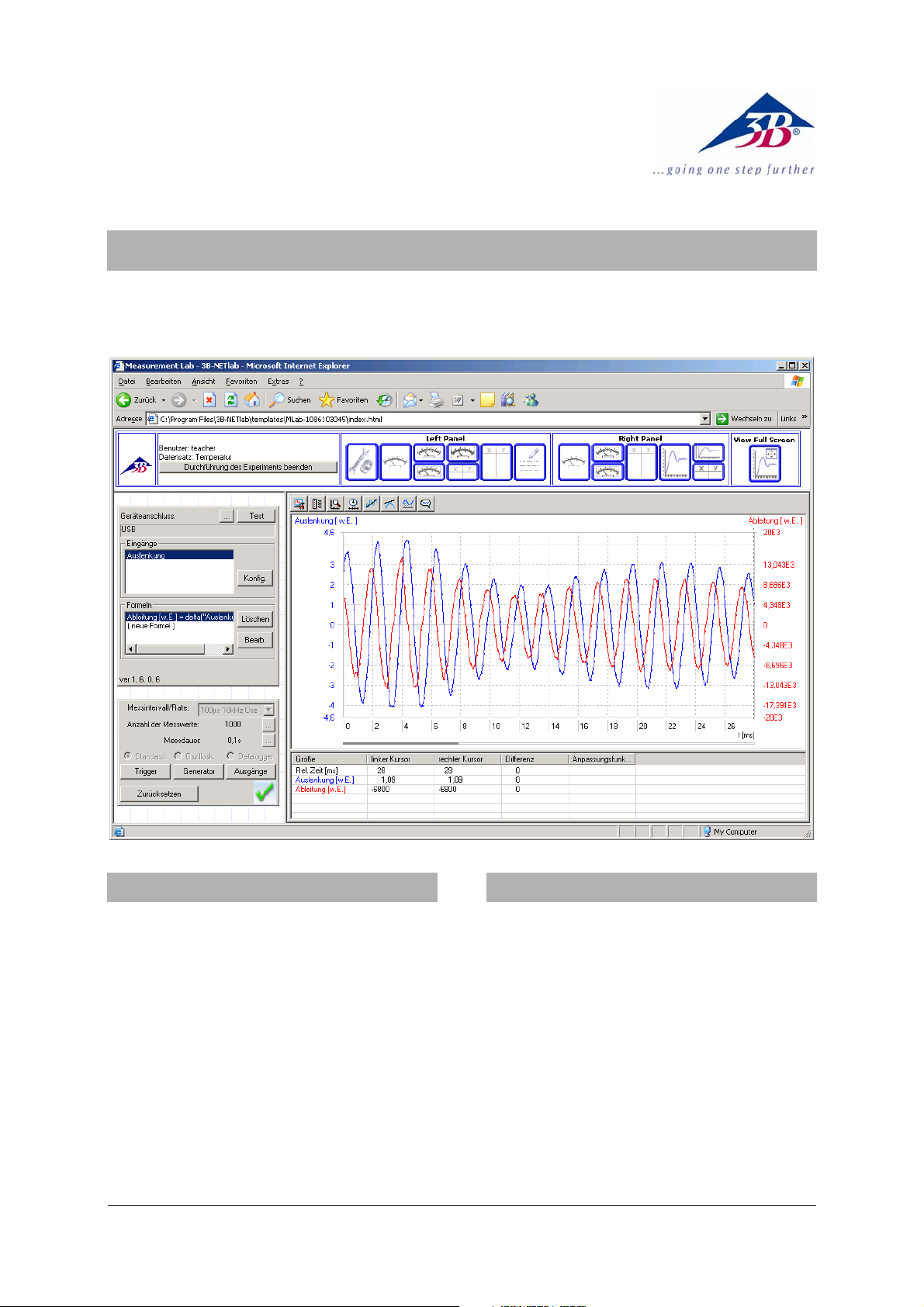
5.1. Measurement lab
(for your own experiments)
5.2. Experiments (instructions)
6. Administration and network set-up
7. Network applications
8. Support
1 Introduction
3B NETlab™ is a data collection and evaluation
program for the 3B NETlog
that can be incorporated into a network. Since it is
based on ActiveX technology, all its control elements can be integrated into web pages which can
be displayed and operated using Microsoft’s Internet Explorer browser.
The main function of the 3B NETlab
facilitate computer-aided experimentation for
educational purposes. To this end, instructions for
numerous experiments from the various areas of
physics are available in web-page form. A user can
navigate between pages just as on the internet and
can use controls connected to on-site equipment to
conduct all aspects of the procedures.
TM
(U11300) equipment
TM
program is to
1
Page 2

A measurement lab has been provided from which
all functions of the 3B NETlog™ equipment can be
operated. To evaluate the measured data, the program is equipped with a whole range of graphic
tools.
Thanks to its networking functionality, the
3B NETlab™ program is perfectly suited for application in schools and educational institutes. Instructors are able to monitor the progress of students
and the data they gather during experiments from
their own workstation. Similarly, students can follow experiments being demonstrated or carried out
by an instructor on their own monitor screens.
2 System requirements
2.1 System requirements
• Windows 98/ME/2000/XP
• Microsoft Internet Explorer 6 or later
• Intel Pentium III/AMD Athlon 600 MHz or
higher
• 128 MB RAM
• 50 MB hard-disk storage
• Monitor with 1024x768 resolution or higher
• USB connection
2.2 Additionally recommended
• Internet access
• Adobe Reader 7.0
• Adobe Flash Player
3 CD-ROM contents
• 3B NETlab™ software
• USB driver
• Instruction manual
4 System set-up and installation
4.1 System set-up:
In order to ensure flawless functioning of
3B NETlab™, it may be necessary to alter certain
settings for Microsoft’s Internet Explorer which are
connected to the execution guidelines for ActiveX
controls.
4.1.1 ActiveX controls:
An ActiveX control is a software program that cannot run independently. Rather, it is executed in a
container provided by a separate application. The
most prominent example of such an application is
Microsoft’s Internet Explorer with its capability to
display ActiveX controls on web pages. This is
mostly used for integrating multimedia content
(e.g. animations using Adobe's Flash Player). Since
ActiveX controls can provide any kind of functionality within programs regardless of the container,
this technology offers users far greater possibilities
(e.g. on Microsoft’s Windows Update website, where
updates can be installed into the operating system
via an ActiveX control). At the same time, however,
there are also certain dangers accompanying this
technology – for instance, risks due to dubious
websites which attempt to plant and execute harmful program code in the form of ActiveX control
elements onto the user’s computer. For this reason,
Internet Explorer is so configured that it requires by
default the explicit consent of a user before installing a control. A publisher or server can be verified
on the basis of a digital signature. If such a digital
signature is missing, any attempt by a website to
install code is ignored.
4.1.2 Security settings for Internet Explorer:
The 3B NETlab™ control is provided with a digital
signature and can thus be installed by Internet
Explorer without altering the default settings. As a
rule, it is only necessary to alter the settings
marked * to allow the program to run. However, if
a particularly restrictive security policy has been
instituted, then further modifications may be required.
Internet Explorer differentiates between various
security zones: “Internet”, “Local intranet”, “Trusted
sites” and “Restricted sites”. To modify the settings,
go to the “Tools” menu, select “Internet Options”
then click the “Security” tab.
Since the pages for 3B NETlab™ are present either
on the hard-disk of the local computer or on the
local network, it is likely that the zone that requires
new settings is the one called “Local intranet”.
If the standard level has been set to “Medium”,
“Medium-low”, or “Low”, no further steps are re-
quired. If not, set the following settings under
“Custom Level”.
• “Script ActiveX controls marked safe for script-
ing” – “Enable”
• “Run ActiveX controls and plugins” – “Enable”
• “Active scripting” – “Enable”
There is no specific zone for pages on the local
computer. In order to permit the execution of
ActiveX control elements, go to “Security” and activate the following option in the “Advanced” tab
(Windows XP only):
• “Allow active content to run in files on My
Computer” *
If you use a pop-up blocker, deactivate the blocker
when working with 3B NETlab™, since the system
works with pop-ups.
2
Page 3

4.2 Installation:
The following steps will guide you through the
installation of 3B NETlab™ for single-user operation. Installation on a network is described in chapter 7.
4.2.1 Driver installation
Before installing the 3B NETlab™ software, it is
important to install the USB driver:
• Connect 3B NETlog™ to the computer via the
USB cable.
The computer reports that it has detected a new
hardware. Subsequently, the window of the hardware wizard opens:
• Insert the installation CD into the CD-ROM
drive of the computer.
Windows 2000:
• Select “Search for the best driver for your de-
vice”.
• Under search for driver files, select “CD-ROM
drives”. (If no driver can be found, select “Display other source locations”.)
Windows XP:
• Do not activate Windows Update.
• Select “Install software from specified loca-
tion”.
• Under “Browse”, specify the location of the
driver on the CD.
• A hardware message will state that the soft-
ware has failed to pass the Windows Logo Test.
You should nevertheless click “Proceed with installation”.
As an alternative, the folder containing the driver
file can be copied directly onto the computer from
the CD and can be installed from the hard disk.
4.2.1.1 Exception:
If the software for the U21800 CCD linear camera
and/or U21830 Spectrophotometer products has
already been installed onto the computer, follow
the instructions below:
• Connect 3B NETlog™ to the computer via the
USB cable.
The computer will not report that a new hardware
has been detected.
• Insert the installation CD into the CD-ROM
drive of the computer.
Windows 2000:
• System control panel -> System -> Hardware ->
open Device manager.
• Double-click USB controller.
• Double-click “ULICE USB Product”.
• Click Driver -> Update driver. (The wizard for
updating the device driver will start.)
• Select “Show all known drivers from list and
search for the suitable/appropriate driver”.
• Select “Drive” and then “Search” to establish
the path to the driver.
• Click “Yes” to confirm that the file should be
overwritten.
Windows XP:
• System control panel -> System -> Hardware ->
open Device manager.
• Double-click on USB controller.
• Double-click “ULICE USB Product”.
• Click Driver -> Update driver. (The hardware
assistant will start.)
• Do not activate Windows Update.
• Select “Install software from specific source”.
• Select “Do not search. Autodetect driver”.
• Select “Drive” and then “Search” to establish
the path to the driver.
• Click “Yes” to confirm that the file should be
overwritten.
• Click “Proceed with installation” when the
hardware message states that the software has
failed to pass the Windows Logo Test.
4.3 Software installation
1. Insert the Install CD into the CD-ROM
drive.
2. If the install program does not start auto-
matically, run “start.exe” from the root directory of the CD-ROM or right click the
CD-ROM drive icon and select “AutoPlay”.
3. Click “Install 3B NETlab™”.
4. A window appears in which you can select
a language by clicking on the respective
country flag. In response to the prompt
“Install 3B NETlab?”, click “Yes”.
5. Click “OK” to start the installation.
6. The program raises the question whether
the directory “C:\Programs\3BNETlab”
should be created, click “Yes”.
7. Enter a user name and password for the
instructor (or the program administrator).
Click “OK” to confirm.
8. The program files will then be installed.
3
Page 4

9. A window appears in which you can select
the experiments that are to be installed.
These experiments have been categorised
according to language and subject area. It
is possible to select either individual experiments or whole categories. Select the
required experiments/categories and click
“OK” to confirm.
10. The experiments will now be installed.
11. After completion of the installation, a
message box appears stating “Installation
completed successfully. Click OK to launch
program”. Click “OK” to confirm.
12. Internet Explorer will now be restarted
automatically and the program will be
loaded.
5 The experiment system
3B NETlab™ differentiates between two types of
experiments. On the one hand, it features a series
of experiment procedures covering various disciplines of physics. By following the instructions
therein, experiments can be conducted quickly and
purposefully using predefined settings. On the
other hand, the measurement lab lets you access
all settings and functions for the 3B NETlog™
equipment in order to conduct your own experiments.
Once the program has been started by either clicking the desktop icon or via the Start menu, a
prompt appears. You should now log in by entering
your user name and password. You can now select
from among the following items:
• Measurement lab
• Experiments
• Administration
Details for Administration are explained in chapter 6. The procedure after selecting either of the
first two items is very similar, since the measurement lab, in principle, also provides a set of instructions for experiments, the only difference
being that it leaves all options open. The steps
required for starting an experiment, managing the
experiment data and operating controls are thus
explained here using the measurement lab for all
examples. These then apply equally to the “Experi-
ments” option.
5.1 Measurement lab (for experiments of your
own design):
5.1.1 Starting, suspending, resuming and com-
pleting experiments:
5.1.1.1 Starting an experiment:
You can start the Measurement Lab by selecting
the corresponding item from the splash screen
then clicking “Continue”. You will now see a list
with the available data entries. A data entry or
record contains all the information on the status of
a particular experiment as well as the measurements made hitherto. To start a new experiment, it
is necessary to create a new data record.
1. Select “Create new data set” and click “Con-
tinue”.
2. Enter a name for the data record and click
“OK” to confirm.
A new measurement lab window then opens. Before dealing with the controls featured in the
measurement lab and the experiments themselves,
further explanation is required on how to proceed
with the data records.
5.1.1.2 Suspending and resuming an experiment;
importing, exporting and deleting data records:
It is possible to suspend the experiment at any time
that no actual measurement is being made.
1. Simply close the experiment window. The
program will then return to the main window.
2. Click “Back”.
The data record you created now appears in the
list. The status “executable” indicates that it is
possible to resume the corresponding experiment
by selecting the item “Open selected data set”.
Furthermore, options for deleting, exporting and
importing data records are also provided.
To export a data record set, it is necessary to specify a directory in which system components as well
as experiment data can be copied so that the experiment can be resumed from this location.
5.1.1.3 Concluding an experiment:
As soon as the first measurement has been concluded in the course of an experiment, a button
“Finish the experiment” appears in the top left hand
corner of the window.
1. Click the button to deactivate all measure-
ment functions.
2. Close the experiment window.
3. Click “Back” in the main window.
The data record is now marked is now marked
“Finished” and can be opened only for viewing.
4
Page 5

5.1.2 Measurement functions:
5.1.2.1 Establishing and testing a connection:
In the first row of the upper left hand control panel
(Input control panel) in the measurement lab window, it is possible to enter the name of the connection by which the 3B NETlog™ is linked to the computer by using the “…” button. This setting need
only be modified in exceptional cases. Normally, it
is set to “USB”. By clicking the “Test” button, the
connection can be tested and the result is displayed after a brief pause.
5.1.2.2 Selection of inputs:
Selection of the inputs required for measurements
can also be carried out in the top left control panel.
Clicking “Select” opens a dialog box, in which the
desired inputs can be specified. The following options are available:
Analog input A: used for measuring voltage, current or other quantities in conjunction with a sensor box which can be connected via the input at
the side.
Analog input B: used for measuring voltage or
other quantities in conjunction with a sensor box
which can be connected via the input at the side.
Digital inputs: the four digital inputs of the
3B NETlog™ unit are integrated together in an 8-pin
mini DIN connector on the right and designated A,
B, C and D. It is possible to interpret the inputs in
any of the following ways:
• As individual signals (A, B, C or D)
• An OR of all four signals (1 if at least one of the
signals is HIGH)
• The binary number represented by the signals
(“D/A conversion”, 1•A + 2•B + 3•C + 4•D)
Manual input: by selecting this input type it is
possible to enter a value into the data record
manually.
Time: a pulse signal at any of the digital or analog
inputs can be processed to determine information
about the pulse with regard to its timing. A value is
recorded for every pulse.
• Pulse time: elapsed time from the beginning of
the measurement to the rising edge of the current pulse.
0
t
• Puls duration: elapsed time between the rising
edge and the falling edge of the current pulse.
t
• Pulse distance (- +): elapsed time between the
falling edge of the previous pulse and the rising edge of the current pulse.
t
• Pulse distance (+ +): elapsed time between the
rising edge of the previous pulse and the rising
edge of the current pulse.
t
Frequency: measures the mean frequency or duration of a periodic signal at an analog or digital
input over an interval specified by the user (the
start and end of the interval are specified by activating a button.)
5.1.2.3 Configuration of inputs:
The selected inputs appear in a list at the top of the
control panel. In order to configure a specific input, select it and click “Config”. A dialog box appears which provides various options depending on
the selection:
Analog inputs:
• Symbol/Name and description: this makes it
possible to rename an input (e.g. corresponding to the quantity which will be measured)
and also allows a description to be entered, if
needed, that should follow a semicolon.
• Input mode: selects between sensor (for use
with an external sensor box), DC voltage (VDC),
rms AC voltage (VAC), DC current (IDC, analog
input A only) and rms AC current (IAC, analog
input A only) measuring modes.
• Input range: selection of input range (measur-
ing range)
• Use prefix for displaying values: this makes it
possible to display measured values, large or
small, with prefices in front of the unit instead
of expressing them in powers of 10.
Digital inputs:
• Input mode: selects between displaying the
signal for a single input (digital signal A, digital
signal B, …), the result of ORing all four signals
(arbitrary digital signal) or the binary number
represented by the four signals (D/A conversion, MSB: D).
Time/frequency:
• Input mode: selects the input where the pulse
signal is to be measured. The following selections are possible: digital input A, an OR of two
5
Page 6

or more digital inputs (A, B), (A, B, C), (A, B, C,
D) or either of the analog inputs. If the analog
inputs are selected, an additional check box
appears for setting a comparator threshold
(see below).
• Input range:
Digital inputs: assigns logical states to physical
input signals. “Uninterrupted = 1” means that
high voltage (>3.8 V) at the input corresponds
to a logical 1 and low voltage at the input
(<0.3 V) corresponds to a logical 0. The relation
is reversed if “Uninterrupted = 0”. This notation is derived from the status of a light barrier
associated with the digital input.
Analog inputs: (see above)
• Comp. level: sets a threshold voltage, specified
as a percentage of the upper limit of the input
range. The threshold voltage denotes the point
of transition between the two logical states.
By using the data conversion table on the right
hand side, it is possible to define how you want a
value to be displayed in relation to the actual signal. This relation is described by means of a table
consisting of pairs of values. Enter pairs of values
for the measured value and the value to be displayed starting from the bottom and working up.
Enter the unit for the new value in the “Results”
box. During subsequent measurements, instead of
the directly measured value the value displayed
will be converted with the help of the table. Values
between the entries in the table will be interpolated assuming a linear gradient between entries.
5.1.3 Formulas:
Underneath the input control panel is another
panel in which it is possible to enter formulae that
are based on the measured values. This function is
mostly used when the values of a particular quantity are to be displayed together with the measured
values. The quantity to be displayed is a function of
the measured quantity, i.e. its values can be calculated directly from the measurements.
• In order to enter a new formula, select “(New
Formula)” from the list and click “Edit”. .
• In the dialog box which appears, enter the
name of the value to be calculated in the
“Formula name” field and the corresponding
unit in “Formula unit”.
• To define the formula, use variables and func-
tions from the two lists that are provided by
double clicking the “Formula text” field. Note:
the term representing the measured values is
entered in the formula in inverted commas.
The check box “Use prefix” makes it possible to
display formula values using prefices instead of
expressing them in powers of 10.
After clicking “OK” to confirm the entries, the formula name is added to the list. When this is se-
lected, the formula can be edited or deleted by
means of the corresponding buttons.
5.1.4 Control of measurements:
After selecting inputs and entering formulae, click
“Inputs OK” on the input control panel to confirm
the entries. You can now proceed with adjusting
settings for recording measurements via the control
panel underneath (Measurement control panel).
Various logging/recording modes can be implemented depending on the selection and configuration of the inputs. First of all, however, it is important to define the recording speed (sampling rate)
in the field “Sampling rate”. The entries set the
interval between two recordings or, in some cases,
the corresponding frequency. AC current or voltage
measurements, i.e. measurements of root mean
square values, or measurements involving several
sensors can only be carried out in a slow mode
(interval >
0.5 s).
The final option is for manual mode (“manual
sampling”), in which recording of a measurement
is triggered by clicking a button.
The following three recording modes are available:
Recorder: a pre-defined number of measurements
are carried out. This number can be specified directly via the field “Number of measurements” or
indirectly via the duration of the measurement (set
using the adjacent “…” button). At a sampling rate
of 100 Hz or less, the measured values are output
in real time as the measurements are made. In
high-speed mode (>100 Hz), the data is first stored
in the internal memory of the equipment and read
out after measurements have been completed. It is
possible to view the measured values in various
ways, e.g. as a graph or in tabular form.
Oscillosc.: the measurements are recorded over
time and displayed as a curve. After each sweep
from left to right, the old curve is replaced by a
new one. Unlike standard mode, in oscilloscope
mode only the last 128 measurements can be
viewed or stored. Since a new trace is recorded only
a few times per second, at high-speeds oscilloscope
mode only displays samples of the overall signal
waveform. However, the advantage over standard
mode is that, even in high-speed mode, it is possible to observe measurements in “real time”.
Datalogger: it is also possible to record measurements offline using 3B NETlog™, without being
connected to the computer. The necessary configuration can be selected on the equipment itself or
conveniently using this function in 3B NETlab™.
After completing measurements, once the device is
connected to the computer again, the data can be
read out via the same function.
Use the “Trigger” button to open a dialog box that
defines the trigger conditions that initiate recording in standard mode.
6
Page 7

• Activate the inputs which are to be triggered at
the left of the box.
• In the middle of the box you can select
whether the trigger should occur when the signal crosses the threshold rising or falling.
• Trigger thresholds for the analog inputs can be
set on the right (as a percentage of the upper
limit of the input range).
5.1.5 Conducting measurements:
When all settings have been carried out, confirm
and click “Parameters OK”. You can now start
measuring by clicking “Start”.
5.1.5.1 Standard mode:
• If manual recording mode has been selected,
you can make a measurement simply by clicking “Sample”. At high -speeds a bar appears
showing the progress of the measurements being conducted. The display of measured values
is dealt with in section 6.1.8 “Evaluation”.
• Measurements can be stopped before they
have finished by clicking “Finish”. If this is not
done, measurements continue to be made until the desired number of values has been recorded. After that it is possible to carry out an
evaluation.
• In order to start new measurements, first click
“Reset”. You will first be given the chance to
save the current recorded values in a new data
record. Thereafter, you can begin conducting
new measurements. In case any parameters
need to be changed, click “Change settings” in
order to return to the choice of inputs. Your
saved settings will not be overwritten by doing
this.
5.1.5.2 Oscilloscope:
A new window opens, consisting of the oscilloscope
display and control panel. It is possible to adjust
the sampling rate and the input range by moving
the corresponding sliders during measurements. In
addition, a trigger is provided which initiates the
recording of the measurements when the threshold
has been crossed. The first slider, marked “Trigger”
in the control panel, is used for selecting the trigger
input. The second slider determines in which direction the threshold has to be crossed. The third
slider sets the threshold itself, specified as a percentage value of the top limit of the input range.
The “Sampling” control panel allows you to choose
between “Single” and “Continuous” modes. If “Sin-
gle” has been selected, the recording of measurements begins when you click “Start” and ends after
one sweep. In this manner, it is possible to trace
rare events as soon as they cause a trigger without
their being immediately overwritten.
The oscilloscope window can be closed by clicking
either of the buttons “Abort” or “Finish and Store
Data”. If you click the latter, the measurements
most recently recorded (128 samples) remain displayed in the display mode selected at the top, just
as in standard mode, and are available for evaluation.
5.1.5.3 Datalogger:
In this mode, no measurements are actually begun
after you click “Start”. Instead, a selection window
appears.
Setup: writes the configuration of the inputs and
the sampling rate to the equipment. Once a message has been received acknowledging that the
data has been stored, the equipment can be disconnected from the computer and can be used as a
portable device for measurements. Additional
information is available in the 3B NETlog™ instruction manual.
Readout: this opens a second selection window.
Click “Readout” to read data from the internal
memory of the 3B NETlog™ device. “Previous data”
calls up the most recently recorded data. A list
containing the available data records appears, from
which it is possible to select one set of records and
download it by clicking “OK”. Note: the maximum
number of samples read out is no greater than the
value that was specified under “Number of samples”
in the measurement control panel.
5.1.6 Generator:
5.1.6.1 Constant signals and digital pulses
In the course of the measurement process voltage
signals can be output from the analog outputs and
logical signals from the digital outputs. The “Out-
puts” button accesses a menu where you can enter
values for constant voltage at the analog outputs.
For digital outputs, it is possible to choose between
the following options:
0: During the entire measurement process, the
digital output is set to “logical 0” (0 V).
1 permanent:
during the entire measurement
process, the digital output is set to “logical 1” (5 V).
1 with delay: the digital output switches to “logi-
cal 1” shortly after the measurement process has
been started.
Pulse with delay: the digital input sends a pulse
shortly after the measurement process has started.
In order to activate the analog outputs, turn on the
check box “Analog outputs ON”.
5.1.7 Signals varying over time (Function genera-
tor):
It is possible to use the function generator to generate time-variant periodic signals at the analog
outputs using the “Generator” button. The sample
rate for the generator is always equal to the sampling rate of the measurement. If manual recording
has been selected, then the sampling rate of the
7
Page 8

generator can be set in the corresponding input
box of the “Sampling” panel. Next to this is the
check box “Generator enabled” that enables the
function generator.
The type of signal can be defined separately for
Channel A and Channel B by selecting the corresponding output. Clicking “Predefined” opens a
dialog box in which one of the following predefined signal waveforms can be selected: “Sine”,
“Rectangle”, “Triangle” and “Flat”. The parameters
are also modified according to the selected type of
signal. Click “OK” to confirm the entries. The specified signal is then displayed in a graphic.
It is possible to use the mouse to plot arbitrary
signal types on the graph. Move the cursor to the
left edge, press the left mouse button, draw the
desired signal with the cursor and release the
mouse button after you have finished.
The period and frequency of a repeating signal are
displayed above the graphic.
If the same signal is to be output to both outputs,
set the signal for output A and click “Copy from A”
under “Channel B” (or vice versa).
Note that the function generator is not working in
the oscilloscope mode.
5.1.8 Evaluation:
5.1.8.1 Display of measurements:
After any measurement in standard or oscilloscope
mode, the data can be viewed in various forms. It is
possible to change the display at any given time by
simply clicking the corresponding icons at the top
edge of the screen.
Dial: the current value is displayed on a
dial as on an analog multimeter. This
representation is useful at slow speeds or
in manual mode because the currently
valid measurement can be displayed in
real time.
Dual display: the values of two inputs
are displayed simultaneously.
Table: a table containing the measured
values is displayed
Selects the columns to be displayed
Copies the selected measured data
records to the clipboard
Manual entry of values in the se-
lected cells
Deletes all manually entered values
Graph: the measured values are plotted
on a graph. The next section deals with
the functions available for the graphical
display.
Table and pointer: see above
Graph and table: see above
Notes: This allows you to enter com-
ments describing the measurements.
Settings: once a display setting for the
left-hand side of the screen has been
configured, clicking this icon allows the
control fields to be reopened for modification.
5.1.8.2 Graphical display:
In a graphical display, the data for each digital
input is displayed in a different colour with a legend underneath. The parameters for the x-axis are
entered in the first row.
The graph provides two cursors represented by
vertical dotted lines that can be moved along the xaxis. Just move the mouse close to one of these
cursors, press the left mouse button and move the
cursor to the requisite position, releasing the cursor
when it is correctly placed. The coordinates of the
cursor are displayed in the row containing the
legend for the x-axis. Beneath that, the individual
measurements are contained in the rows corresponding to the y-axis, i.e. the y coordinates for the
selected curve at the cursor position.
The right mouse button is used for zooming. A
context menu appears which provide the possibility
of zooming in or out of the x-axis, the y-axis or
both of the axes. It is possible to highlight sections
by keeping the right mouse button pressed and
dragging the mouse, thereby enclosing the relevant
section in a rectangle. The contents highlighted
within this rectangle can be magnified to fill the
entire screen by selecting “Zoom into selected win-
dow”. The visible section of the graph can be
shifted by dragging the axis legend with the left
mouse button.
A row of icons is located above the graph. The
following sections explain their function:
Setup display: (connecting lines, grids, data
points, etc.)
Select inputs/formulas to be displayed: also
for assigning what is to be on the x-axis. The x-axis
8
Page 9

can also be assigned to one of the measured values
(x-y display).
Modify scale range: use “Autoscaling” to
scale the highlighted axis so that it is possible to
view all data. “Manual scaling” opens a dialog box
in which the limits of the visible intervals can be
entered manually.
Modify time scale range: (exception: in x-y
mode, both of the axes are set in the dialog box
described above)
Fit to a function (Fit): for further information
see the following section
Calculate tangent: if this icon is activated,
then a tangent is drawn to the displayed curve
from the last cursor to be moved If several curves
are visible, then it is necessary to select one of the
curves in a selection window before proceeding.
The section of the axis and the gradient of the
tangent are displayed in the upper left of the
graph.
Calculate integral: when this icon is activated, it is possible to calculate the integral of the
highlighted (or the only visible) data curve within
limits defined by the cursors. In graphical terms
this corresponds to the area below the respective
curve (which is shaded). Any areas below the x-axis
are considered negative.
Edit text labels: activating this icon allows us
to create a text field and position it on the graph.
5.1.8.3 Fitting to a function (Fit):
Proceed as described in the following to fit a function to a data curve:
• Click the icon for the graph. A dialog box
for fitting the function will open.
• On the left, select the desired data.
• Click “Edit fit function for selected quantity”.
A window appears in which the section of the
curve that was highlighted earlier by the cursors is drawn (preview) and a list of functions is
presented.
• Select the desired function from the list or
define a unique function by means of “Edit the
user formula”. (See section 6.1.3 “Formulas”. It
is possible to use six parameters from A to F.
The independent variable appears last in the
list.) The equation (strictly speaking, the right
hand side of the algebraic equation) of the
chosen function is displayed above the list.
• Specify the parameters for the initial values on
the right hand side. This is not always necessary. Sometimes, however, the preset initial
values are not helpful. Click “Draw” to plot the
function with the specified parameters in the
preview.
• In addition to the input fields for the initial
values, activating the check box can cause the
parameter values to remain constant during
the fitting of the function.
• Click “Try to fit”. The result is displayed in the
preview. The correlation coefficient R
2
is output
above the control panel labelled “Parameters”.
• After clicking “OK” and exiting the window for
fitting the function, the fit function is also plotted on the graph.
An existing fit function can be edited in the same
way. In order to display or hide a fit function, open
the dialog field for setting a fit function and, after
highlighting the relevant data set, click the corresponding icon.
5.2 Experiments (according to the instructions):
The only difference between experimenting according to instructions and experimenting with the
measurement lab is that the control panels have
been incorporated and pre-configured in the experiment procedure. Usually, only those measurement functions which are significant are activated.
In this way, even users little accustomed to the
functions of 3B NETlog™ are able to perform experiments easily. To begin an experiment, proceed
from the splash screen as follows:
• Select “Experiments” and click “Continue”.
• Choose “Perform/browse an experiment” and
click “Continue”.
• Select an experiment from the list and click
“Continue”. The experiment which is now visible is recognised by the measurement laboratory. This is where the data pertaining to the
selected experiment are administered. Subsequently proceed as explained in section 6.1.1.1
“”.
6 Administration and network set-up
The functions of 3B NETlab™ described in the following section support its operation within a network. After installation, no administrative intervention is required for single-user operation. Owing to
the innumerable ways of implementing a network
and the corresponding differences in configuration
associated with that, it is not possible to explain
the various steps in detail within the scope of this
chapter. Administrator rights are essential for setting up a network.
The network functionality makes it possible for
instructors to observe students’ experiments from
their own computer while they are being conducted and also to view the recorded readings.
Likewise, instructors can also conduct an experi-
9
Page 10

ment at their own computer while students observe at their terminals.
Communication is conducted entirely via Windows
file sharing. No additional TCP connections need to
be set up. The supervisor can regularly access and
read a data file shared by the computer where the
experiment is being conducted. The data is thus
accessible from the supervisors’ controls after only
a very brief delay. At the same time however, supervisors are not restricted to viewing those pages
or controls currently being used by students performing the experiments. A supervisor can, for
instance, check the individual numbers in a table
while the student performing the experiment is
conducting an analysis of them in a graph.
6.1 Network installation:
Installation on an instructor’s computer is carried
out as in the single-user installation procedure, but
subsequently the instructor’s computer is set up as
a server.
• Select “Administration” from the splash screen
and click “Continue”.
• Select “Adm. the teacher's server and student's
computers” and click “Continue”.
• Select “Define/modify the teacher's
server” and click “Continue”.
• In the dialog box, a path is displayed which
must now be shared for all network users to
have read access. For NTFS data systems, make
sure that the necessary authorisation is
granted.
• Enter the network address of the share. Click
“OK” to confirm.
A message appears which explains how to proceed.
Among others, the URL for the installation of the
3B NETlab™ students’ version is specified. The following steps must be carried out on each student’s
computer. While carrying out these steps, make
sure to observe the notes on security settings, as
described in section 4.1.2.
• Enter the installation URL in Internet Explorer.
• An installation prompt appears for the ActiveX
control element “3BNETlab” which you should
accept.
• The installation routine for the students’ ver-
sion begins. Confirm the creation of a program
directory.
• A message appears in which the path is speci-
fied. This must be shared in order to grant the
instructor full access. Make sure the relevant
authorisation is provided for NTFS file systems.
After confirming this message, the program is concluded. It is now important that the server can
detect the student computers. To test this:
• Go to “Administration” and select the item
“Define a new student's computer”. Click
“Continue”.
• Enter a name and the network address of the
supervisor share on the student’s computer.
Click “OK” to confirm.
6.2 User identification for students:
A separate user ID can be set up for each individual
student. The advantage of this is that after logging
on for each experiment, only that particular student’s data are listed. In this way, any confusion
which may arise on account of multiple students
working simultaneously is avoided. Also, experimental results are always ascribed to a particular
student. This simplifies the task of monitoring for
the supervisor.
6.2.1 Setting up user identification for students:
After the installation of the network, students must
be granted user identification in order to run the
program.
• From “Adm. the teacher's server and
student's computers” click “Back” to return
to the previous page.
• Select “Students” and click “Continue”.
• Select “Create new student entry” and click
“Continue”.
• From the list, select the computer on which the
user ID is to be created and click “Continue”.
• Enter a user name for the student.
• Select a user group. If necessary, click “Create
a new group of students”.
• Enter a password. Click “OK” to confirm.
6.2.2 Changing students’ user identification:
• Go to “Students” and select “Edit an existing
student entry”.
• From the list of students’ entries, select an
entry then click “Modify” and “Continue”.
• A dialog box appears where it is possible to
change the group and, if required, the password of the student.
6.2.3 Deleting students’ user identification:
• Go to “Students” and select “Edit an existing
student entry”.
• From the list of students’ entries, select an
entry then click “Delete” and “Continue”.
6.3 User identification for teachers:
6.3.1 Setting up user identification for teachers:
It is also possible to set up an individual user identification for each teacher.
10
Page 11

Go to “Administration”. Select “Administrate
•
the teachers' list” and click “Continue”.
• Select “Create a new teacher entry” and
click “Continue”.
• Enter a user name and password, click “OK” to
confirm.
6.3.2 Changing your own password:
Any teacher can only change his/her own password.
• Go to “Administration”. Select “Administrate
the teachers' list” and click “Continue”.
• Select “Edit current teacher entry” and click
“Continue”.
• Activate the “Change” check box in the field
labelled “Password”.
• Enter a new password. Click “OK” to confirm.
7 Network applications
This chapter describes functions which can only be
used in the network.
7.1 Teachers monitoring experiments con-
ducted by students:
Experiments conducted by students can be monitored at any time by the instructor. Even after
completion of the experiment, it is still possible to
refer to and consult the data.
• Select “Administration” on the splash screen
and click “Continue”.
• Select “Student” and click “Continue”.
• Select “Watch a student’s experiment” and
click “Continue”.
• From the list, select a particular student whose
experiment you wish to monitor and click
“Continue”.
• From the list, select the data sets you wish to
see. The “Date/time” column specifies the time
the data set was created.
• Click “Browse”. The experiment window will
open. However, the control elements are deactivated. Therefore, it is not possible to take
control of the experiment.
While monitoring an experiment, it is possible to
change the display or navigate on the page independently, without interfering with the participating student(s). The evaluation functions of the
graph display may also be used.
To exit the experiment, simply close the window
and click “Back” to return to the main window.
7.2 Students observing experiments conducted
by teachers:
It is possible for the students to observe experiments conducted and demonstrated by the instructors.
• Select “Watch the teacher's experiment”
on the splash screen and click “Continue”.
• From the list, select the data sets you wish to
see. The “Date/time” column specifies the time
the data set was created.
• Select “Browse”.
The experiment window will open. It provides the
same range of options as described under section 7.1 “Teachers monitoring experiments conducted by students”.
8 Support
If you have any queries and/or suggestions, please
feel free to contact our support team:
Email: support@3bnetlab.com
3B Scientific GmbH • Rudorffweg 8 • 21031 Hamburg • Germany • www.3bscientific.com
Subject to technical amendments
© Copyright 2009 3B Scientific GmbH
Page 12

 Loading...