YSI 6200 User Manual

YSI incorporated

6200
Data Acquisition System

User’s Manual

Table of Contents

Page

Section 1 Introduction

1.1 Description 1-1

1.2 General Specifications 1-2

1.3 How to Use this Manual 1-4

Section 2 Getting Started

2.1 Unpacking and Inspection 2-1

2.2 Installing EcoWatch DCP 2-2

2.3 Setting Up System Components f or Checkout 2-3

2.4 Setting Up a 6-Series Sonde for System Checkout 2-6

2.5 Configuring the System 6200 with EcoWatch DCP 2-11

2.6 Testing the 6200 DCP 2-16

2.7 Testing Sensor Function 2-19

2.8 Displaying Data in EcoWatch DCP 2-21

Section 3 Setting Up and Calibrating 6-Series Sondes

3.1 Introduction 3-1

3.2 Communicating with a Sonde 3-1

3.3 Connecting a Sonde to a Computer with EcoWatch DCP 3-3

3.4 Preparing the Sonde to Communicat e with the 6200 DCP 3-4

3.5 Installing and Calibrating Sonde Sensors 3-5

Section 4 Powering the Field Station

4.1 Introduction 4-1

4.2 General Wiring Information 4-1

4.3 Installing the Battery 4-4

4.4 Installing AC Power to the Field Station 4-5

4.5 Installing Solar Power to the Field Stat ion 4-7

Section 5 Connecting Sensors to the Field Station

5.1 Introduction 5-1

5.2 Connecting the MET Suite 5-2

5.3 Connecting the Rain Gauge 5-2

5.4 Connecting the Pyranometer 5-3

5.5 Connecting One Sonde 5-3

5.6 Connecting More Than One Sonde to a Field Station 5-4

Section 6 Communicating with the Field Station

6.1 Introduction 6-1

6.2 Installing RS232 Direct Communication Link 6-6

6.3 Installing RF Radio Communication Link 6-7

6.4 Installing Phone modem Communicat ion Link 6-9

6.5 Installing Cellular modem Comm unication Link 6-10

6.6 Setting Up Communication Paramet er s with EcoWatch DCP 6-11

3

Section 7 Collecting Data with EcoWatch DCP

7.1 Introduction 7-1

7.2 Completing Field and Base System Setup 7-1

7.3 Verifying Field/Base Communication from the Field 7-3

7.4 Collecting Data with EcoWatch DCP 7-3

7.5 Reconfiguring Sensors and System with EcoWatch 7-11

7.6 Backing Up and Restoring DCP Configuration Files 7-14

Section 8 Reporting and Plotting Data with EcoWatch DCP

8.1 Introduction 8-1

8.2 Opening a Data File 8-1

8.3 Viewing Data 8-3

8.4 Changing Display Formats Using Setup 8-7

8.5 Changing Display Formats Using ‘Gr aph’ Funct ion 8-8

8.6 Save, Import, Export and Print Comm ands 8-9

8.7 Example of Customizing a Subset of SAMPLE.DAT 8-10

Section 9 Maintaining and Troubleshooting the System

9.1 Introduction 9-1

9.2 Routine Care and Maintenance 9-1

9.3 Troubleshooting 9-5

Appendix A Component Descriptions and Sensor Specifications

Appendix B Required Notice

Appendix C Warranty and Service Information

Appendix D Accessories

Appendix E Field Installation Examples

4

Assistance

Help with this product can be obtained by contacting a YSI Factory Service Center.

United States

YSI Massachusetts
Repair Center
13 Atlantis Drive
Marion, MA 02738
Phone: [phone]
Fax: [phone]

Compliance

The 6200 Data Acquisition System meets the EN61326 Electronic Equipment for Measurement
and Control specification when connected 6-series sonde cabling is protected from RF induction
and industrial noise. The 6-series sondes may malfunction over the frequency range of 4.2 MHz
to 8.5 MHz at a level of 3 volts RF on the cable (see Appendix E).

The 6-series sonde must be fitted with the CE bead kit for the 6200 system to meet the Class B
emissions requirements.

The 6200 complies with EN61010 as manufactured.

1

Safety Notes

The following type of safety notes are used throughout this manual. Familiarize yourself with
each of the notes and their meaning before using this product.

NOTE The NOTE is used to indicate a statement of company recommendation or

policy. A NOTE is not associated directly with a hazard or hazardous
situation, and it is not used in place of CAUTION or WARNING.

CAUTION! Used to indicate a hazard. It calls attention to a procedure that, if not

correctly performed, could result in damage or injury. Do not proceed
beyond a caution sign until the indicated conditions are fully understood
and met.

WARNING! Used to indicate a hazard. It calls attention to a procedure that, if not

correctly performed, could result in injury or loss of life. Do not proceed
beyond a caution sign until the indicated conditions are fully understood
and met.

General Safety Considerations

WARNING!

No operator serviceable parts inside. Refer ser vicing t o a YSI factory service center.

To prevent electrical shock, do not remove covers.

This is the instruction documentation symbol. The product is marked with this
symbol when it is necessary for the user to refer to instructions in this manual.

2

YSI 6200 DAS USER Manual

Section 1

Introduction

1.1 Description

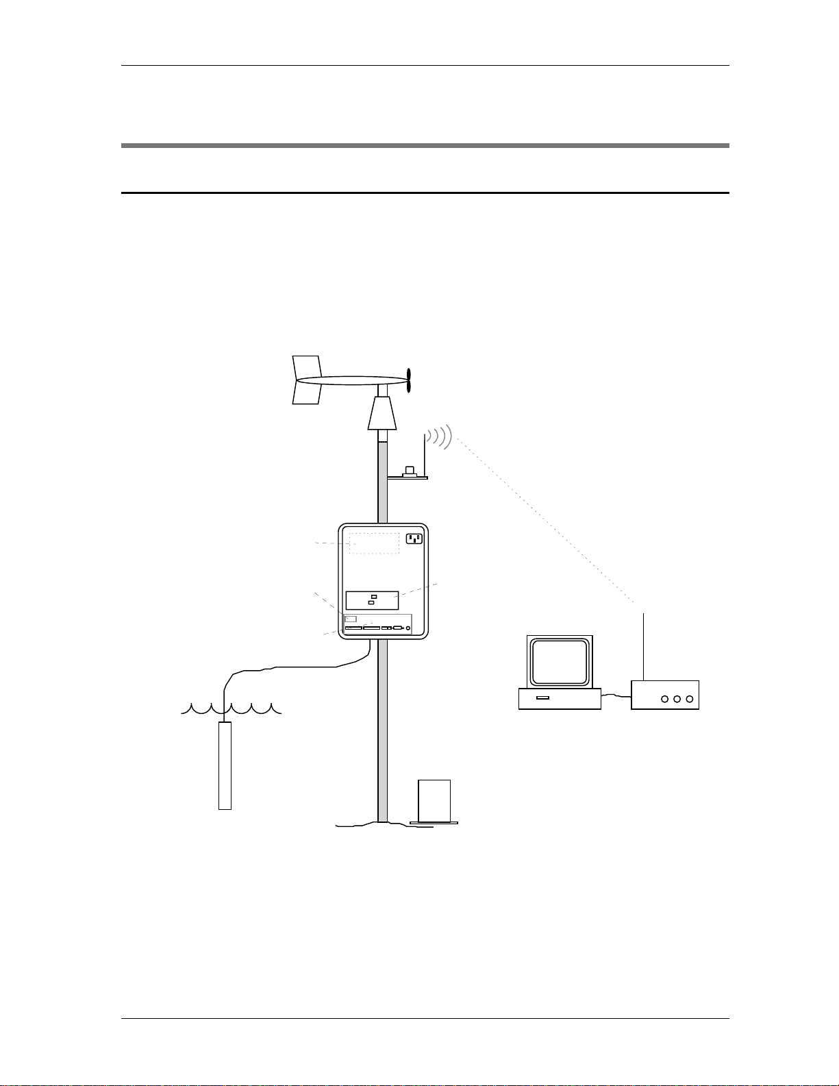
The 6200 Data Acquisition System (6200 DAS) with EcoWatch DCPä is an integrated hardware
and software package specifically designed to be a powerful, yet easy to configure, multiparameter
water quality and meteorological data collection platform with a graphical user interface.
Information can be collected real-time or periodically from solid state memory. Combined with
YSI 6-series sondes and/or a variety of meteorological sensors, this system is intended for use in
research, assessment and regulatory compliance applications.

Wind Speed/Direction
Relative Humidity
Air Temperature

Radio
Antenna

Solar
Radiation

Radio Transceiver

Battery
(charged Solar or AC)

Computer with
EcoWatch DCP

Rain accumulation
Rain rate

Radio
Base Station

6200
Data Collection Platform

6-Series Sonde

Barometer

Water Temperature
Conductivity
Dissolved Oxygen
pH
ORP
Depth/Level
and more...

Figure 1.1 6200 DAS, Example Config uration

The system can be configured many ways, using a variety of sensors, communication modes and
power options. The sensors provide signals for both water quality and meteorological
measurement parameters. The meteorological sensors include wind speed and direction, relative
humidity, barometric pressure, rainfall rate and accumulation, air temperature and solar radiation.

YSI/Massachusetts 508.748.0366, Fax [phone] Page 1-1

YSI 6200 DAS USER Manual

The water quality sensors include water temperature, conductivity, dissolved oxygen, pH, ORP,
depth/level, turbidity, nitrate, ammonia and chloride.

The system includes a field station (6200 DCP), which houses a powerful data logger and connects
to any of the water quality or meteorological sensors you choose. The data logger uses a 32-bit

â

microprocessor with up to 1 megabyte of data storage memory. Windows

-based EcoWatch DCP
software functions to interrogate the data logger and display real-time results in time stamped table
format. Alternatively, you may request data stored in the field station less frequently to conserve
power. The software also provides autoconfiguration capability during setup and calibration and
includes a powerful plotting package for further analysis of the recorded data.

There are four options for communication between the field station and the base station computer.
They are (1) direct link via RS-232 serial communication, (2) phone modem communication, (3)
cellular phone communication, and (4) UHF radio communication.

There are three options for powering the field station. They are (1) rechargeable lead acid battery
(12 volt, 12 Ah) mounted inside the NEMA 4X field station enclosure, (2) solar panel that charges
the battery described in 1 above, and (3) 100/120//220/230-240 V~, 50/60 Hz power. The battery
is installed in all versions. It is required in the solar setup and serves as a backup in the AC power
setup.

The 6200 DAS comes to you configured to your order, including all interface cables. You may
need to provide additional wiring and junction boxes if you are powering the field station with AC
power. You may need to provide mounting supports for the main enclosure and various
accessories, such as sensors, antennas and the like. Most of the mounting hardware you need
comes with the 6200 system, but some may not be appropriate for your particular mounting
configuration.

The 6200 DAS specifications are described below. You may refer to Appendix A for
specifications of specific sensors and accessories. In addition, the accessory manuals provided
with this manual package should be helpful.

1.2 General Specifications

Environmental

Operating Temperature -40 to 60oC (-40 to 140 oF)
Enclosure 33 x 38 x 15.2 cm (13 x 15 x 6 in), fiberglass
Enclosure Rating NEMA 4X
Pollution Degree II (per UL3101)
Installation Category III (per EN61010-1)

Data Acquisition

6200 DCP (standard) 64 KB RAM, 56 KB required for run-time memory

8 KB (logging memory)

Memory Options 256 KB, 200 KB (logging memory)

1 MB, 968 KB (logging memory)

YSI/Massachusetts 508.748.0366, Fax [phone] Page 1-2

YSI 6200 DAS USER Manual

User-Interface

Software YSI EcoWatch DCPä featuring autoconfigurable sensors,

real-time data displays, powerful reporting and plotting options
Compatibility: Windows

â

3.1, 95, 98 and NT.

Computer Hardware Minimum: PC 386 (4 MB RAM, 4 MB hard disk space)

Recommended: PC 486DX or higher, (8 MB RAM, 4 MB hard
disk space)

Power Information

Battery Type Lead-acid, gel type, sealed (Power Sonic PS-12120 L)
Battery Rating 12 VDC, 5 A max current, 12 Ah capacity
Battery Fuse Type/Rating Type 3AG (fast blow), 5 amps, 32 volts
I/O Interface Fuse Type/Rating Type 3AG (slow blow), 5 amps, 32 volts

When applicable…

Line Power (nominal) 100/120//220/230-240 V~, 50/60 Hz, 0.8A//0.4A
Maximum Current 1.0 A @ 120 V~, 0.5 A @ 240 V~
AC Fuse Type/Rating for 100/120 V~ operation: Type 3AG (slow blow), 1.0 A @ 120 V
AC Fuse Type/Rating for 220/240 V~ operation: 5 x 20mm IEC127 (time delay), 0.5 A(T), 250 V

Fuses may be purchased from any YSI Factory Service Center.
Solar Panel 10 watt, 20 VDC (no load), 0.6 A max current
Electrical Safety CE (pending)

Communication Options

Direct cable 3 m (10 ft) RS-232 cable
Radio 2 watt, 2-way (no license required), 467.8 MHz
Telephone modem Hayes-compatible
Cellular modem Wireless phone modem, uses PSTN through cellular network

Connectors/Access

Power (AC or solar) 1/2” non-metallic, water tight conduit or feed through gland

AC, 3-prong male; Solar, 2-wire interface cable
Phone or direct 1/2” non-metallic, water tight conduit or feed through gland

Phone, standard 3-wire cable; Direct RS-232, DB-9 male
RF (radio or cellular) N-type
Sonde MS-8 pin with tethered cap
Meteorological Suite MS-17 pin with tethered cap
Rain Gauge MS-4 pin with tethered cap
Solar Radiation Sensor MS-5 pin with tethered cap
Ground Standard Ground Lug

Sensor Compatibility

Sonde Compatibility YSI 600, 600R, 600XL, 600XLM, 6820, 6920.
Met Suite (WS, WD, RH, AT) YSI MAZ6213, w/ 4.6 m (15 ft) cable
Met Suite (WS, WD, RH, AT) YSI MAZ6219, w/ 13.7 m (45 ft) cable
Pyranometer (solar radiation) YSI MAZ6214, w/ 3 m (10 ft) cable, leveling base
Pyranometer (solar radiation) YSI MAZ6212, w/ 3 m (10 ft) cable, leveling base, CE approved
Rain Gauge (tipping bucket) ISCO 674, w/ 4.6 m (15 ft) cable
Rain Gauge, with heater YSI MAZ6216, w/ 4.6 m (15 ft) cable (also requires AC power)
Barometer YSI MAZ6217, (located inside NEMA enclosure)

YSI/Massachusetts 508.748.0366, Fax [phone] Page 1-3

YSI 6200 DAS USER Manual

1.3 How to Use this Manual

The 6200 DAS is a complex product that requires your understanding before y ou can successfully use
it; therefore, we strongly suggest that you perform the following steps to get y our sy stem set up
quickly and correctly in the field.

Part I Manual Sections to Read

Familiarize yourself with the 6200 DAS 2, Browse through manual
Unpack and setup sonde 3, Sonde Manual
Check out Communication Method 2, 6, 7
Plan out and prepare remote site 4, 5, See Appendix E for samples

Part II

Fully Calibrate Sonde 3, Sonde Manual
Prepare 6200 DCP for the field 7
Go to the field site and setup 4, 5, 6, 7
Verify that the system work s 7, 8

Section 2 Getting Started

After this section you should be familiar with the 6200 DCP, the EcoWatch DC P user­interface software, and the sensors. This “in lab” setup should give you a basic
understanding of the system. The mo re detailed inform ation found in the other sections
is necessary for the installation and day-to- day operation of the system.

Section 3 Setting Up a 6-Series Sonde

If you are using a 6-Series sonde with your system this section provides basic
information related using a Sonde with this package.

Section 4 Powering the Field Station
Section 5 Connecting Sensors to the Field Station
Section 6 Communicating with the Field Station

Section 7 Collecting Data with EcoWatch DCP

This section needs to be read to properly configure the data collection platform. It
includes power management strategies, and how to upload reading s from the data
collection platform.

Section 8 Reporting and Plotting Data with EcoWatch DCP
Section 9 Maintaining and Troubleshooting the System

Throughout this manual the phrase 6200 DAS (Data Acquisition System) refers to the entire 6200
package you have purchased, including the field station, communications methods, and EcoWatch
DCP software. The phrase 6200 DCP (Data Collection Platform) and field s t a t i o n are used
interchangeably and refer to the remote site setup. The phrase base station refers to the office/lab
setup which includes your PC and communication m ethod.

YSI/Massachusetts 508.748.0366, Fax [phone] Page 1-4

YSI 6200 DAS USER Manual

Section 2

Getting Started

2.1 Unpacking and Inspection

Inspect the outside of the shipping carton(s) for damage. If damage is detected, contact the
carrier immediately. Remove the instrument from the shipping container. Be careful not to
discard any parts or supplies. Confirm that all items on the packing list are present. Inspect all
assemblies and components for damage. The basic 6200 DAS is shipped with the following
major components. Some differences may occur based on the configuration you ordered.

❑ Data Collection Platform with barometer, communication and power accessories installed
❑ Battery for powering remote station (packed separately)
❑ Meteorological Suite (WS, WD, RH, AT) with 4.6 m cable, or 13.7 m cable
❑ Pyranometer (3 m cable) or Pyranometer with CE approval (3 m cable)
❑ Rain Gauge, ISCO 674 (4.6 m cable) or Rain Gauge with heating element (4.6 m cable)
❑ Sonde with appropriate sensors, cables, adapters and reagents
❑ Antennas (if applicable)
❑ Radio Base Station (if applicable)

If you ordered a sonde with reagents, the reagents may be shipped separately. See Appendix D
for a complete list of accessories.

If any parts are damaged or missing, contact your factory representative immediately. If you do
not know from which dealer your 6200 DAS was purchased, contact YSI/Massachusetts. See
phone/fax information below in the footer.

Save the original packing cartons and packing materials. Carriers typically require proof of
damage due to mishandling. Also, if it is necessary to return any parts, you should pack the
equipment in the same manner it was received. Maintaining original cartons and packing
material is less critical once the system is installed and working

If the 6200 DAS components match the packing list and the components appear to be in
satisfactory condition, proceed to the sections below.

WARNING!

To avoid severe personal injury or damage to the equipment...installation,

operation and service should be performed by qualified personnel who

are thoroughly familiar with the entir e cont ents of this manual.

The 6200 Data Acquisition System with EcoWatch DCPä is an integrated hardware and
software package. Most of the hardware will be installed in the field. We will refer to this as the
“field” location. The “base” location will refer to the site where the radio base station or modem
connects to the computer loaded with EcoWatch DCP. We strongly recommend that you
assemble the system “in-house” and functionally test it prior to beginning the field

YSI/Massachusetts 508.748.0366, Fax [phone] Page 2-1

YSI 6200 DAS USER Manual

installation of the system. The next few pages of the manual describe the checkout installation.
You need not use the final mounting hardware to perform this test, however, this is a good time
to review your installation plan for your field site.

2.2 Installing EcoWatch DCP

Choose a computer with these minimum requirements: 386 processor with 4 MB of RAM, at
least one COM port and Windows
you will need at least 4 MB of available hard disk space. Although these minimum requirements
work, we recommend a 486DX processor with 8 MB of RAM and 2 COM ports. The EcoWatch
DCP software is also fully compatible with the Pentium
Windows NT
Windows 98

To install on Windows 3.1:

â

. The system has also been designed and tested with current beta versions of

â

.

Insert Disk 1 into your 3.5” drive. From Program Manager, click on File, then

choose Run. In the box labeled Command Line type in “a:\setup.exe” then click on
OK. If the disk is in drive B, change the command to “b:\setup.exe”. Follow the

instructions and prompts on the screen to complete software installation. Once complete,
store your disks in a safe place in the event you need to reload the software at a later
date.

To install on a Windows 95 or NT machine:

Insert Disk 1 into the proper drive, then click on Start at the bottom left of the screen,

then Run from the submenu. In the box type in “a:\setup.exe” then click on OK. If the
disk is in drive B, change the command to “b:\setup.exe”. Follow the instructions and
prompts on the screen to complete software installation. Once complete, store your disks
in a safe place in the event you need to reload the software at a later date.

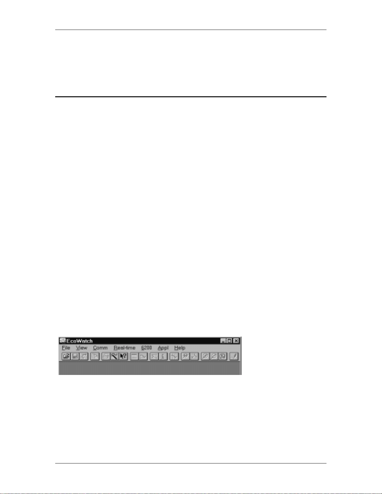
When you double click on the EcoWatch DCP icon, the main screen will display a window with
menu bar and icons similar to the one shown below. Below is a Windows 95 illustration.
Windows 3.1 will look slightly different, but not be functionally different.

â

3.1. A 3.5” disk drive is needed to load EcoWatch DCP, and

â

processor and Windows 95â and

There are limits to what you can do with EcoWatch DCP at this time, so you should now turn
your attention to making hardware connections. If part of your 6200 DAS includes a sonde, your
first use of EcoWatch DCP software will be to communicate with the sonde to set sensors and
report parameters and to calibrate the sonde. This is described below in Section 2.4.

YSI/Massachusetts 508.748.0366, Fax [phone] Page 2-2

YSI 6200 DAS USER Manual

2.3 Setting Up System Components for Checkout

In this section you will find instructions for checkout installation of your entire system in the
laboratory or other temporary location of your choice. Field station and base station components
will be in the same room for this initial setup and checkout procedure. Your setup may differ
from the one described below since the 6200 DAS was ordered to your specification. Many
steps are common to all setups, therefore simply skip sensor, communication and power setup
instructions that are not relevant to your system. Section 5 will go into more details about setting
up each sensor in the field.

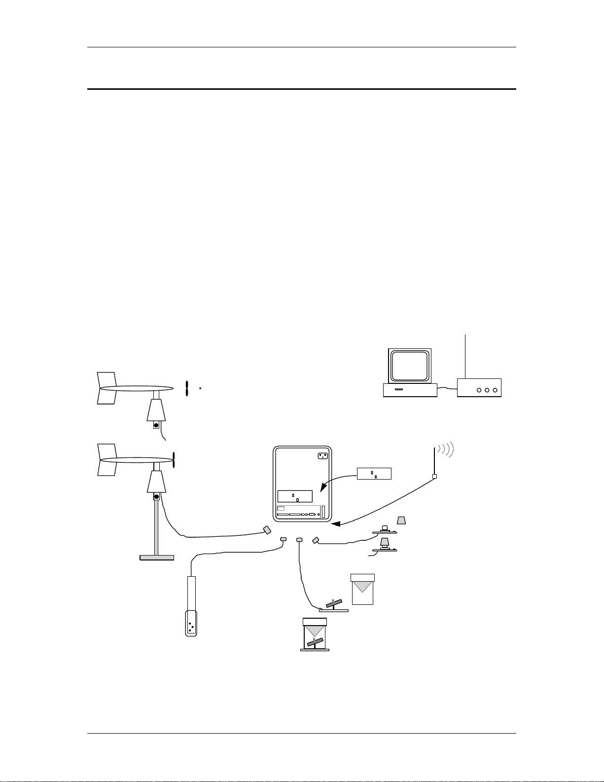
The example 6200 DAS described below contains all of the standard meteorological sensors and
one sonde with the most common water quality sensors. Initially we will use a “Direct Link”
(RS-232) communication option and battery power to set up and check out the system in the
laboratory. If a radio transmitter has been installed in the 6200 DCP enclosure, then it is very
important to install the radio antenna. For this reason the radio and antenna have been shown in
the diagram below. Begin by studying this diagram, then follow the step-by-step assembly and
connection instructions. If your system includes a 6-series sonde, you may want to refer ahead to
Section 2.4 for initial setup information.

MET Suite

Wind Speed/Direction
Relative Humidity
Air Temperature

6200 DAS Components

(Phone Mo de m)

Radio Tra ns ceiver
(or Cel lu l a r Mo dem)

Data Collection
Platform

Barometer

makeshift
support

6-Series Sonde

Water Tempe rat ure
Conductivity
Dissolved Oxyg en
pH

Rain Ga uge

Rain accumulation
Rain rate

Figure 2.1 Lab Setup for Checking Out the 6200 DAS

Computer with
EcoWat c h DCP

AC Power

Battery

Desiccant Pack

Radio
Base St ation

Radio
Antenna

Pyranometer
Solar Radiation

YSI/Massachusetts 508.748.0366, Fax [phone] Page 2-3

YSI 6200 DAS USER Manual

Assuming that all shipping cartons have been opened and the equipment has been initially
checked for damage, proceed by doing the following.

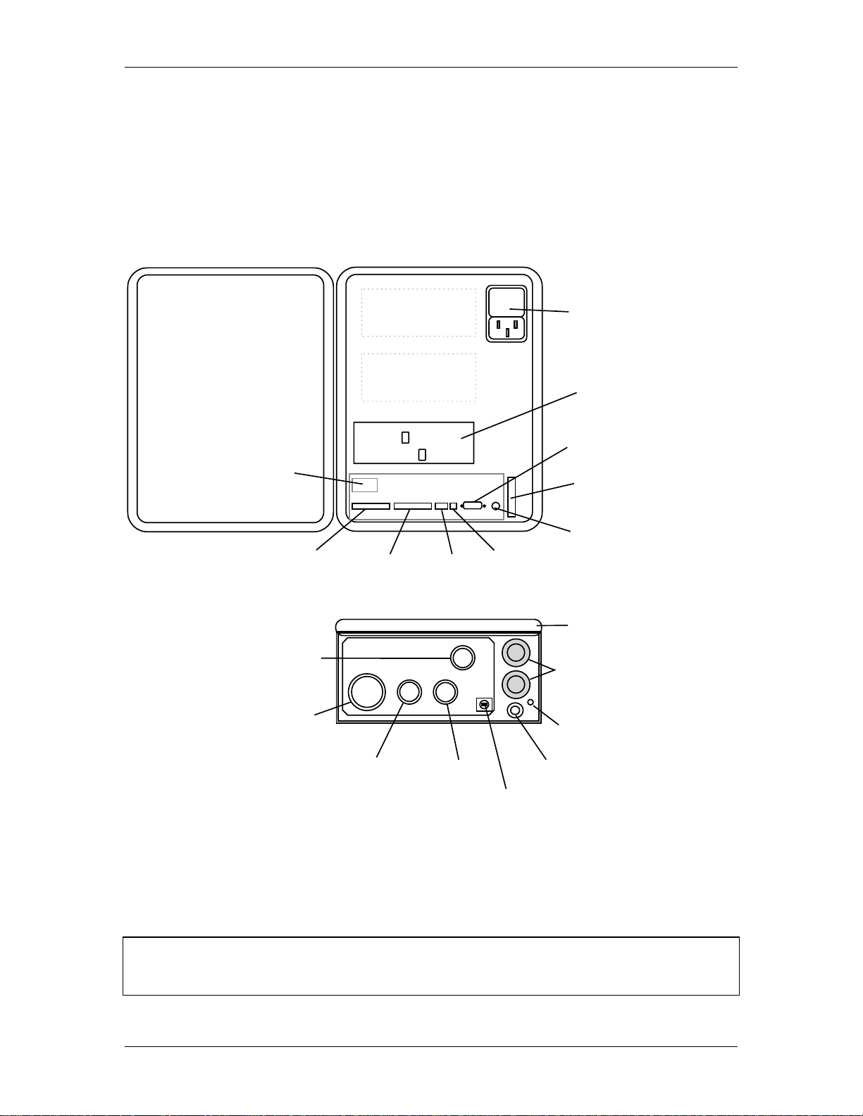
1. Place the 6200 Data Collection Platform enclosure on a work surface, leaving space for

accessories to be laid out and connected. Position the enclosure so that the bottom (connector
ports) faces toward you. Next open the hinged cover, by releasing the two latches on the right
side. Refer to the diagram below, and remember that the diagram may differ slightly from your
unit based on the components you ordered.

Barometer

Analog Inputs

6-Series Sonde

Met Suite

Phone Modem

Radio or
Cell Modem

Digital I/O

bottom view of enclosure

Phone Solar Power In

AC Power In

Battery

COM Port

Desiccant Pack

Fuse

Front Cover

Conduit Fittings for AC,
solar, and phone lines

Barometer Vent

Rain Gauge

Pyranometer

Grounding Terminal

Antenna or RF cable port

Figure 2.2 6200 Data Collection Platf or m, Component and Connector Layout

2. If a radio is installed in the 6200 DCP enclosure, you should locate the field antenna that you

ordered and connect it to the antenna connector on the bottom of the enclosure.

CAUTION!

To avoid permanent damag e to the radio transceiver, connect the antenna befor e

powering the 6200 DCP or the radio base unit.

YSI/Massachusetts 508.748.0366, Fax [phone] Page 2-4

YSI 6200 DAS USER Manual

3. Unpack the battery and insert it into the battery slot (see Section 4.3 for details). The battery

connectors are different sizes. Connect the leads, red to positive and blue to negative. After the
battery is connected, the 6200 DCP should beep for a few seconds as it boots up. The battery
was charged at the factory and should function without problem for this test. Later we will check
the battery voltage with EcoWatch DCP software.

4. For proper testing of the Meteorological Suite sensors, you should construct a makeshift

support or stand for this accessory. A 2” (5 cm) diameter rigid pipe secured to a base works
well. (refer to Figure 2.1) Remove the Meteorological Suite main assembly from its packing
carton. The propeller has been packed separately in the same carton. Remove the propeller, and
use the finger-nut attached to the main shaft to secure the propeller to the main assembly. The
molded lettering on the propeller should face out or away from the main assembly. Hold the
front cone and slightly rotate the propeller to insure that it drops into the “cross” shaped channel
on the cone. Finally tighten the knob on the main assembly with your fingers. Do not use
excessive force. Connect this sensor to the 6200 DCP.

5. Remove the Rain Gauge from the packing carton. There is no assembly required. You may

want to remove the lid, which is an assembly containing a screen or grid and funnel. In order to
functionally test the rain gauge in the lab, the tipping buckets need to be accessible. In the ISCO
model, unlatch the base and gently remove the cylinder/funnel assembly. In the model
containing a heating element, remove the lid/funnel by lifting it off. Connect this sensor to the
6200 DCP.

6. Remove the pyranometer from its packing carton and place it on a flat surface near the 6200

DCP. Locate the certificate and save this document. It contains a calibration constant that must
be entered during the sensor setup routine in EcoWatch DCP. To perform the functional test you
will need to remove the plastic cap that protects the light sensing surface. Also note that a small
bubble level is permanently installed in the base of this unit. During field installation, this
bubble should be used for proper installation. Absolute “level” is not critical during this initial
setup. Connect this sensor to the 6200 DCP.

7. Remove the 6-series sonde from its packing carton. There are several models of sondes that

can be used with the 6200 DAS. Refer to Section 2.4 in this manual for a basic checkout setup.
Note that this is not the complete setup and calibration procedure you would use for deployment
of the sonde at a field station. EcoWatch DCP contains a menu related to sonde communication.
More information for setup of the sonde is located in Section 3. Wait until section 2.4 to connect
this sensor.

8. There are several options that you may use to initially establish a communication link

between the data collection platform and the PC-based EcoWatch DCP software. The simplest
link at this point is the “Direct Link” using the RS-232 cable provided. Plug one end of this
cable into the DB-9 COM port of the 6200 DCP and the other end to a COM port of the PC
loaded with EcoWatch DCP.

Naturally, you will want to functionally check the 2-way radio link, the cellular modem link,
and/or the phone modem link. Refer to Sections 6 and 7 for more information. For now,

YSI/Massachusetts 508.748.0366, Fax [phone] Page 2-5

YSI 6200 DAS USER Manual

however, use the direct link to functionally check your sensors, power source, and DCP in this
laboratory setup.

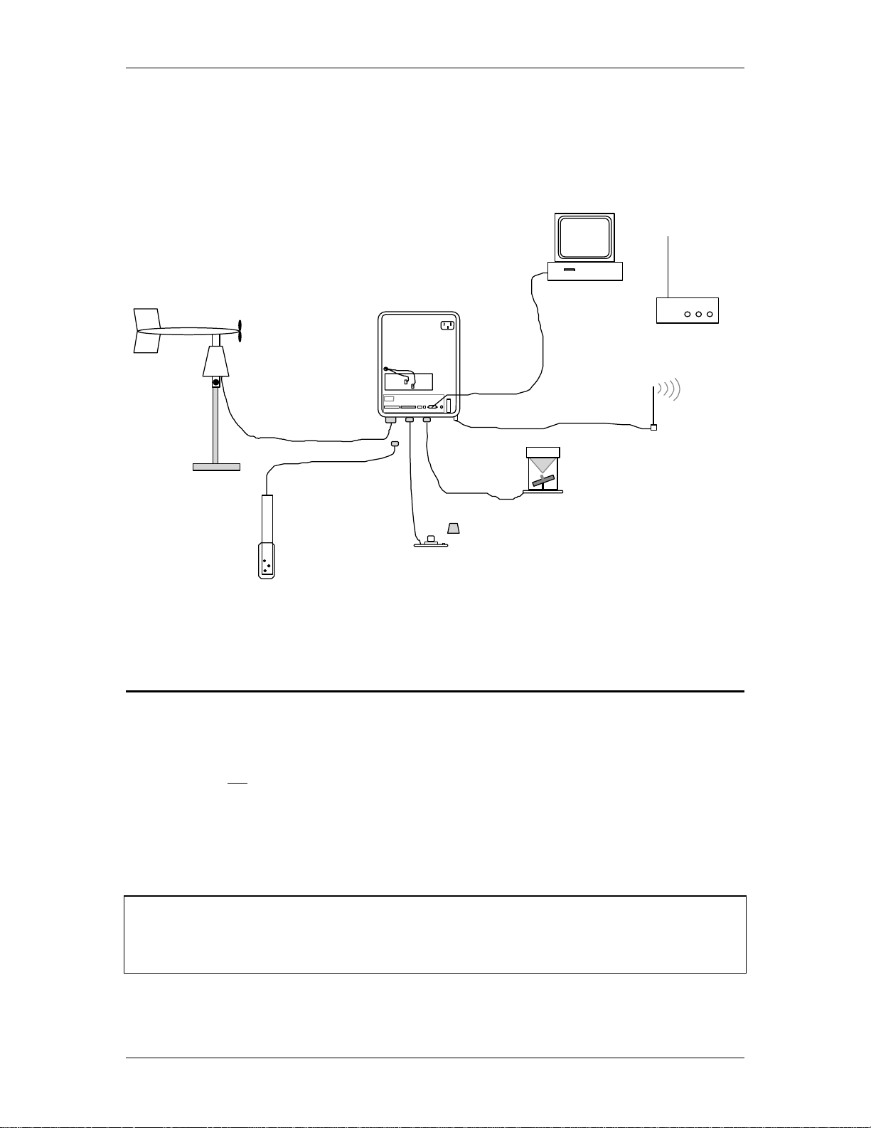
Your setup as described above should now appear similar to the diagram below. Note that the
Radio Base Station is not connected to the system at this point, as it will be checked later.

Direct Link Initial Checkout

MET Suite

Wind Speed/Direction
Relative Humidity
Air Temper ature

makeshift
support

Radio Transceiver
(or Cellular Modem)

(Phone Mode m)

Dat a Col le c tion
Platform

Barometer

AC
Power In

Battery

Computer with
EcoWatch DCP

RS-232
Cable

Radio
Antenna

Rain Gauge

Rain accumulation
Rain rate

Radio
Base Statio n

6-Se r ie s Sond e

Water Temperature
Conductivity
Dissol ved Ox ygen
pH

* Sonde co nnects to MS-8 once calibrated.

*Remove cover to activate tipping buckets.

Pyranometer
Solar Radiation

Figure 2.3 Setup and Checkout Configuration with Direct Link RS-232 (no radio)

2.4 Setting Up a 6-Series Sonde for Checkout

If a 6-series sonde is not part of the system you ordered, proceed to Section 2.5.

Below is the procedure to unpack and set up a 6-Series sonde for 6200 DCP checkout. The

procedure does not include calibration of the sonde sensors. Other than temperature, the
readings may seem unrealistic at this time. The objective is to familiarize you with specific
sensor setup protocols, not to obtain accurate data.

For many sonde models you must physically install some of the sensors into the sonde bulkhead.
You should refer to the sonde manual for details so not to damage the sensors.

CAUTION!

To avoid permanent damag e to the sonde, do not submerse the sonde in water during

this initial checkout.

YSI/Massachusetts 508.748.0366, Fax [phone] Page 2-6

YSI 6200 DAS USER Manual

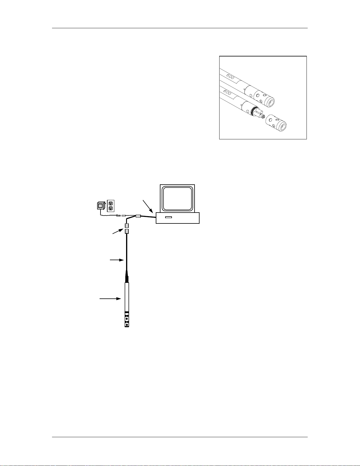
When you remove the sonde from the shipping container, you
will see that a probe guard protects the sensors. Unscrew the
guard to determine the sensors installed. After checking
and/or installing sensors, place the probe guard back in place
to protect the sensors.

Sensors shown in this example are temperature, conductivity,
dissolved oxygen and pH. It is important to know what
sensors are installed for the purpose of correctly assigning
sensors during setup.

Figure 2.4 600 Sonde, Probe Guard Removed

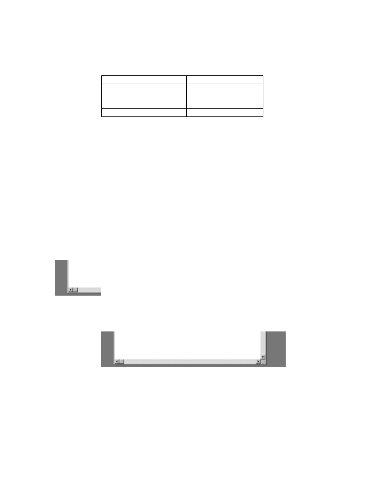
In order to setup your sonde, you must connect the sonde to your PC and communicate through
EcoWatch DCP. The diagram below helps describe this connection.

In addition to the sonde, you need a
cable. The cable may be a field
cable permanently attached to the
sonde or you may need to connect a
separate field or cal cable to the
bulkhead connector of the sonde.

Regardless of the type, the cable

Power Supply
6037: 220 VAC
6038: 110 VAC

MS-8

DB-9

6095B

Adapter

Computer with
EcoWatch DCP

terminates in an MS-8 connector.

Cable

Many sondes also require power in
order to communicate with the PC­based software. A 6095B Adapter
and a 6038 (or 6037) Power Supply

600

600 Sonde

may be needed to make the
connection. The PC-end of the
adapter is a DB-9 which is a typical
COM port connector. If your PC
has a DB-25 connector, you will
need another adapter (25 to 9 pin).

Figure 2.5 Sonde to PC Connection

Identify your COM port, for example, COM 1, COM 2, etc. You need this information to
establish communication between the sonde and EcoWatch DCP. If your COM port is not
clearly marked, assume that it is COM1 for now. You can reconfigure for COM2 (or other COM
port) if communication is not established during setup.

YSI/Massachusetts 508.748.0366, Fax [phone] Page 2-7

YSI 6200 DAS USER Manual

You should now open the EcoWatch DCP program. If you have not installed it yet refer to
Section 2.2, Installing EcoWatch DCP. Click on the Comm top line menu, then Settings…
Verify that the settings match the table.

Baud 9600
Data 8 bits
Parity None
Protocol Kermit
Handshaking XonXoff

Once complete with this window click on OK.
Now return to top line menu and click on Comm, then choose Sonde from the submenu. Select

your COM port and press OK. You will now see a window labeled Sonde – COM1.
The # sign should appear (see below). Type in “menu”. When you press Enter, you will enter
the main sonde menu. It will appear similar to the screen below. Any difference is related to the
model of sonde you are using.

If you are unable to establish interaction with the sonde, make sure that the cable is properly
connected, power is applied (e.g., 6038 Power Supply or other 12 VDC source), and that the
COM port settings are set correctly. If you were unsure of your COM port number, reassign
another port number and repeat the steps above.

YSI/Massachusetts 508.748.0366, Fax [phone] Page 2-8

YSI 6200 DAS USER Manual

The sonde software is menu-driven. Select a function by typing its corresponding number or
character. It is not necessary to press Enter after a number/character selection. Use the 0 or Esc
key to return to a previous menu. The mouse does not interact with the sonde menus.

NOTE

If a single keystroke yields no response on the screen, press the key again. You should

now see a reaction. This occurs when a key is not pressed for a period of time sending

the sonde into a “sleep mode”. The f ir s t pr ess of any key “wakes” up the sonde and the

second press activates the command.

In order to properly assign sensors and parameters for the sonde, follow the step-by-step
instructions below. You need not fully understand each submenu at this time, but you should
configure your sonde menu to appear very similar to the screens shown below. The illustrations
below may differ some from your screens, since sonde menus vary somewhat from model to
model.

1. From Main menu press 3-System, then 1-Comm setup. This allows you to confirm baud
rate at 9600, which is the default value. Refer to the screens below. Note also that the SDI-12
address of the sonde is 0 by default. You may assign any character between 0 and F to provide a
specific address for your sonde. This will be of particular importance in multi-sonde applications
involving the 6200 DAS. For now, maintain the “0” address designation. Press 0 to return to
previous menus until you return to Main.

-----------------Main----------------­1-Run 4-Report
2-Calibrate 5-Sensor
3-System 6-Advanced

-----------System-setup-----------------

Select Option (0 for previous menu):

1-Comm setup
2-Page length=25
3-Instrument ID
4-SDI-12 address=0

Select Option (0 for previous menu):

--------------Comm-setup-------------­1-(*)Auto baud 5-( )2400 baud
2-( )300 baud 6-( )4800 baud
3-( )600 baud 7-(*)9600 baud
4-( )1200 baud

Select Option (0 for previous menu):

2. From Main menu press 5-Sensor, to enter the menu that allows you to assign installed
sensors. In the example we are selecting four sensors which were shown earlier in Figure 2.4.
To change an assignment press the number of the sensor. The * indicates that the sensor is
activated. After assigning sensors press 0 to return to Main.

YSI/Massachusetts 508.748.0366, Fax [phone] Page 2-9

YSI 6200 DAS USER Manual

-----------------Main----------------­1-Run 4-Report
2-Calibrate 5-Sensor
3-System 6-Advanced

Select Option (0 for previous menu):

------------Sensors enabled------------­1-(*)Temperature 5-(*)ISE1 pH
2-(*)Conductivity 6-( )ISE2 NONE
3-(*)Dissolved Oxy 7-( )ISE3 NONE
4-( )Pressure-Abs

Select Option (0 for previous menu):

3. From Main menu press 4-Report, to enter the menu that allows you to assign the parameters
and the units of your choice. In the example we select five parameters...one temperature, one
conductivity, one pH and two for DO. After assigning parameters press 0 to return to Main.

-----------------Main----------------­1-Run 4-Report
2-Calibrate 5-Sensor
3-System 6-Advanced

Select Option (0 for previous menu):

--------------Report setup------------­1-(*)Temp C A-( )Resist Ohm*cm
2-( )Temp F B-( )TDS g/L
3-( )Temp K C-( )TDS Kg/L
4-( )SpCond mS/cm D-( )Sal ppt
5-(*)SpCond uS/cm E-(*)DOsat %
6-( )Cond mS/cm F-(*)DO mg/L
7-( )Cond uS/cm G-( )DOchrg
8-( )Resist MOhm*cm H-(*)pH
9-( )Resist KOhm*cm I-( )pH mV

Select Option (0 for previous menu):

4. From Main menu press 6-Advanced, then 2-Setup. Verify that the screen below matches
what you see. It is very important that the Auto sleep options are activated, especially when the
sonde is being set up for deployment. For more details see Section 3 and your sonde manual.

----------------Advanced--------------­1-Cal Constants 3-Sensor
2-Setup 4-Data Filter

Select Option (0 for previous menu):

-------------Advanced setup-----------­1-(*)VT emulation
2-( )Power up to Menu
3-( )Power up to Run
4-( )Comma Radix
5-(*)Auto sleep RS232
6-(*)Auto sleep SDI12
7-( )Multi SDI12

Select Option (0 for previous menu):

Press 0’s to return to the statement that asks you to press Y or N to exit the sonde menu. Press Y
to exit the sonde menu. Close the Sonde-COM1 window and disconnect the adapters and cables.
Now you should connect the 6-series sonde to the 6200 DCP.

YSI/Massachusetts 508.748.0366, Fax [phone] Page 2-10

YSI 6200 DAS USER Manual

2.5 Configuring the 6200 DCP using EcoWatch DCP

All sensors connect to the 6200 DCP (Data Collection Platform). The DCP electronics
physically reside inside the NEMA 4X enclosure. You should now have all of your sensors
connected and a “direct link” RS-232 cable running from the 6200 DCP a COM port on your PC
(COM1 in our example). You should have an antenna or RF cable connected to the antenna
connector on the 6200 enclosure and you should have installed the battery and connected the
power leads to positive and negative terminals. You are now ready to create a file, configure the
data collection platform, and begin collecting data using EcoWatch DCP. Follow the step-by­step instructions below to proceed.

Start by opening EcoWatch DCP, if it is not already running.

From the main screen click on the top line menu labeled 6200, then click on New... to bring up
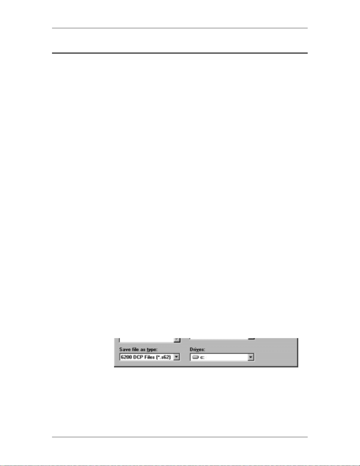
the screen titled “Save 6200 DCP Configuration File As” Type in a filename of your choice (8
character maximum).

In the figure below the filename “checkout.s62” has been entered. Actually three
configuration files (.s62, .zcf, .ini) will be opened and saved in the location shown
(c:\ecowwin\sys6200). You have the option to direct the .s62 file to a location of your choice,
but we recommend that you accept the default path. Click on OK to proceed.

YSI/Massachusetts 508.748.0366, Fax [phone] Page 2-11

YSI 6200 DAS USER Manual

Once you click on OK several status screens will appear indicating that EcoWatch DCP is
attempting to detect the 6200 DCP and its sensors. The screens are part of an autoconfiguration
routine that searches for SDI-12 sensors (sondes) and MET sensors (meteorological sensors).
The screens are titled “6200 DCP ConfigWizard”. An example below shows that a sonde with
SDI-12 Address 0 has been detected after scanning addresses 0 to 8. EcoWatch DCP searches
from Addresses 0 to 9, by default. The sonde with the address of 0 will be the only address
detected in your checkout procedure.

YSI/Massachusetts 508.748.0366, Fax [phone] Page 2-12

YSI 6200 DAS USER Manual

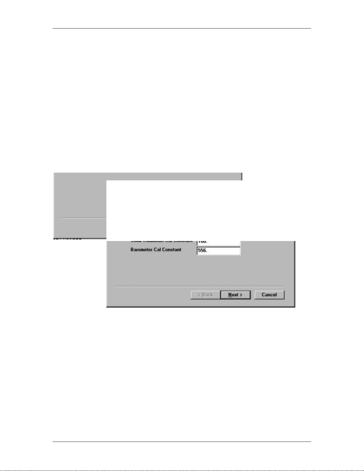
After completing the scan of SDI-12 sensors, the software switches to a ConfigWizard screen
that shows the status of the scan of meteorological sensors. If a MET sensor requires entry of a
calibration constant, a screen appears. Only the solar radiation sensor and barometer sensor
require a calibration constant, which is provided in the sensor literature or included in the back of
the manual. Each time you make a New 6200 file you will need to enter these calibration
constants. A good place to save these calibration constants is with the manual. Below you see
the MET status window and the screen for entering the calibration constants for the solar
radiation sensor (pyranometer) and the barometer.

Enter the numbers from the certificates, then click on Next and proceed to the next screen in
ConfigWizard.

YSI/Massachusetts 508.748.0366, Fax [phone] Page 2-13

YSI 6200 DAS USER Manual

The next choice relates to the communication option that you will be using for this particular file.
For example, if you ordered a system with a 2-way radio, click on the appropriate circle.
Remember that even though you may be “directly” communicating with the 6200 DCP field
station during configuration, you must choose the mode of communication you will use for field

installation.

In our laboratory setup and checkout procedure we will be initially communicating directly via
RS-232 cable. Therefore the default choice shown below is correct. Click on Next to proceed.

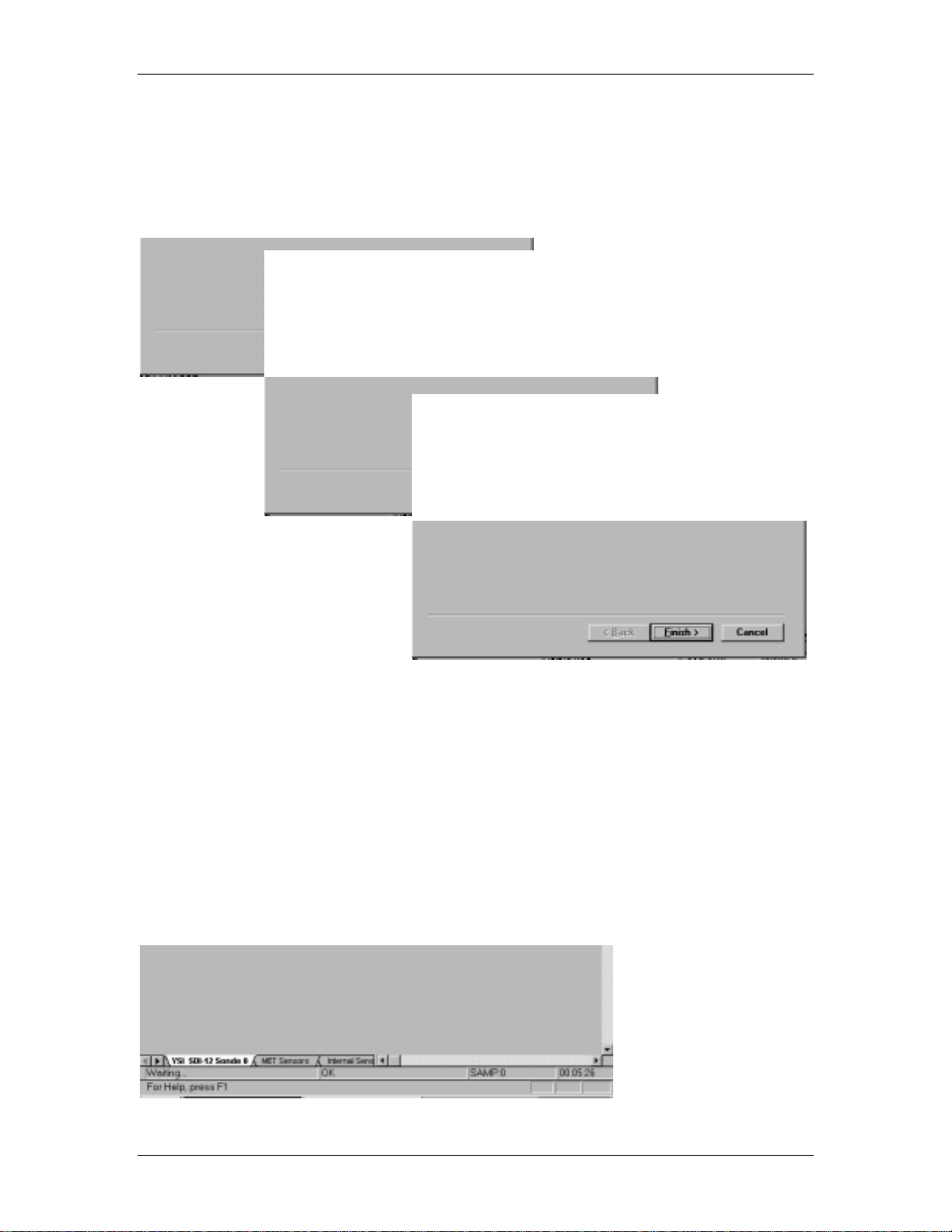
EcoWatch DCP now completes its configuration of the 6200 DCP. See the example screens
below.

YSI/Massachusetts 508.748.0366, Fax [phone] Page 2-14

YSI 6200 DAS USER Manual

The last step EcoWatch DCP will do is to reboot the 6200 DCP, and you should hear a long
beep. After you click on Finish, a report form similar to the one shown below appears on the
screen.

YSI/Massachusetts 508.748.0366, Fax [phone] Page 2-15

YSI 6200 DAS USER Manual

2.6 Testing the 6200 DCP

At this point you have connected the 6200 DCP components, installed EcoWatch DCP and run
the ConfigWizard. You are ready to begin collecting data and display it on EcoWatch DCP. In
order to perform a test that provides data in a timely manner for testing, click on 6200, then
6200 DCP Setup. The following screen should appear.

Click on System… to open the window related to system settings. A message will appear to
alert you that any data remaining in memory in the 6200 DCP will be erased if system settings
are changed. This does not mean that data already uploaded to EcoWatch DCP will be lost. See
Section 7 for more details on the consequences of changing system or sensor settings.

Click on Yes to continue and notice that there are two “folders”, Site/Timing and
Communication/Power. Site/Timing will appear first and the Description box will be
highlighted. By default, it reads <noname100>. The number 100 is the number EcoWatch
DCP has assigned this field station, and may be any number between 100 and 999 since this
value increments each time a new field station is setup. You may type in a description of your
choice or you may tab to the next box, thereby accepting the default description. The next box is
Sample Interval, that is the time that elapses between samples being logged to the data
collection platform (DCP). The default value is 15 (minutes). Do not confuse this with

YSI/Massachusetts 508.748.0366, Fax [phone] Page 2-16

YSI 6200 DAS USER Manual

EcoWatch DCP interrogation timing. Even when EcoWatch DCP is not running, the DCP
continues to log data to its memory once it has been configured.

The next selection gives you the choice of interrogating the DCP at the same rate as the sample
interval or, alternatively, choosing some number of minutes independent of the DCP sample
interval. For the 6200 Test, set the interrogation schedule to “Same as Sample Interval” by
clicking on the box just to the left of this choice. Also change the Sample Interval to 2 or 3
minutes during the checkout routine in order to collect readings more quickly.

1

Now click on the Communication/Power folder and verify that communication is Direct
Connect to PC and the COM port agrees with the serial port to which you are connected

(COM1 in our example screen). The power option should be Battery. The information related
to MODEM communications is not relevant at this point.

YSI/Massachusetts 508.748.0366, Fax [phone] Page 2-17

YSI 6200 DAS USER Manual

Click on OK to exit the menu and return to the main EcoWatch DCP menu screen. A window
appears momentarily, displaying the message Programming 6200...Please Wait. When
EcoWatch DCP is done downloading the new configuration it will reboot the 6200 DCP. You
should hear a long beep from the 6200 DCP as it starts up again.

Once the main menu appears, click on 6200 to pull down the menu and click on Interrogate
Now. Any data that has been collected by the DCP will appear. If readings do not appear
initially, you will need to wait as much time as the sample interval you chose above. A
countdown timer in the lower right corner of the window will give you the time to next
interrogation.

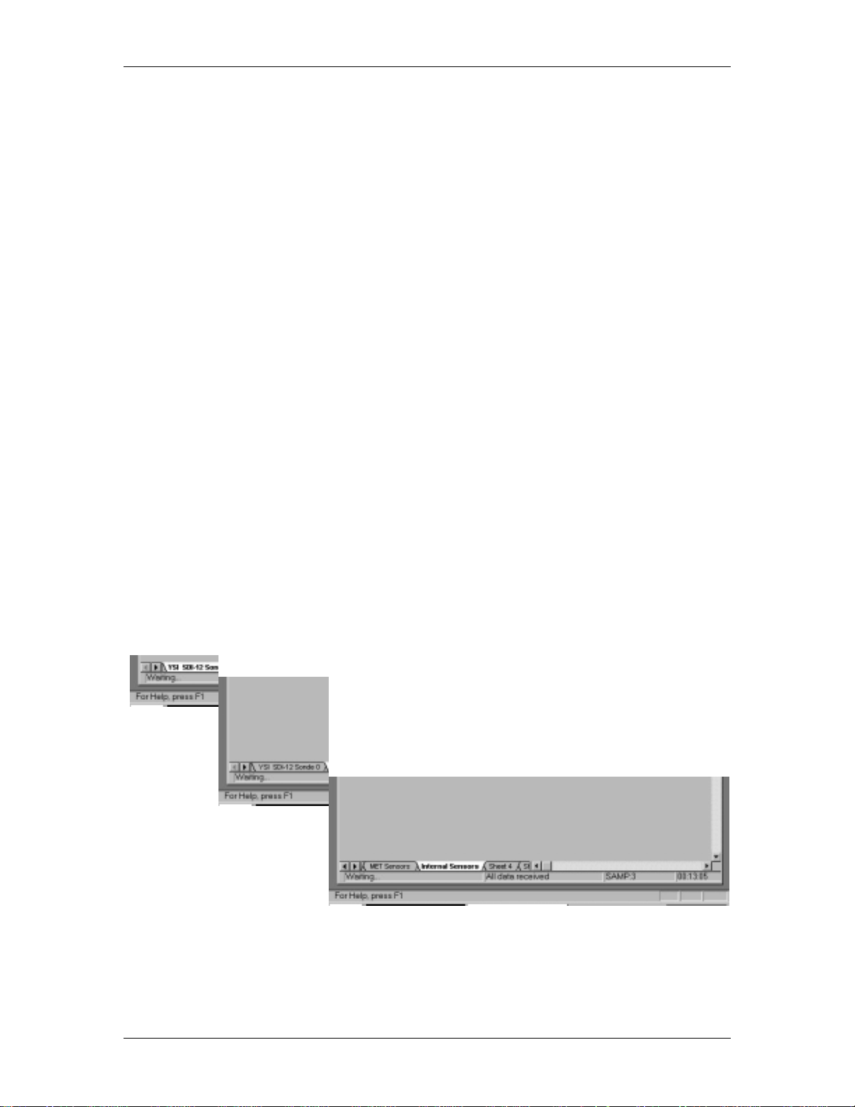
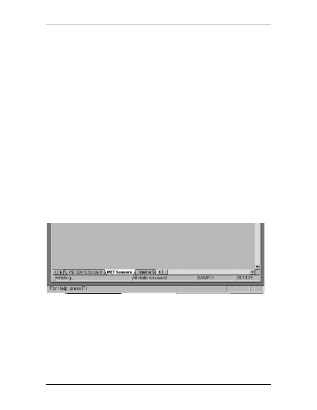
Below you see readings that have been uploaded to EcoWatch DCP from the 6200 DCP. Up to
seven lines of data may be displayed at one time, the bottom line being the most current. Note
that there are three separate display “sheets”. Simply click on the sheet label near the bottom of
each window to view readings from YSI SDI-12 Sonde 0, MET Sensors, or Internal Sensors.
You can not display all sensor readings in one window simultaneously.

YSI/Massachusetts 508.748.0366, Fax [phone] Page 2-18

YSI 6200 DAS USER Manual

If you have difficulty viewing the readings on a sheet, you have two options. One...click and
hold on a vertical line that separates description headers. While holding the mouse button down
you can resize the column width. Two...Click on 6200, Data Table Setup, Font/Color...
The default font/size is Arial/11. Change this to suit your needs. For example, changing the size
from 11 to 9 will fit more information on one screen without the need to scroll.

2.7 Testing Sensor Function

Now that you are able to view readings, you may wish to perform some preliminary tests of
sensor function. As you have seen some readings display 0.000 in the checkout testing. For
example, rain fall and accumulation, wind speed and direction and solar radiation probably have
zero readings. Here are some quick tests you can perform.

For wind speed/direction locate the plastic arrow protruding from the MET Suite head assembly.
Rotate the MET head assembly on the support so that the arrow points north (0 degrees). East
would be 90, south 180 and west 270 degrees. Direction will not be displayed unless there is
measurable wind speed. To check wind speed set up a small fan to provide continuous air
motion in front of the propeller. During interrogation of the 6200 DCP, EcoWatch DCP will
upload readings showing wind speed and direction. In the example below the wind speed is
about 5.4 mph and the direction is 0

For rain rate/accumulation testing, remove the top assembly of the rain gauge to locate the
tipping buckets. Carefully tip the buckets from one position to the other 5 to 10 times in

YSI/Massachusetts 508.748.0366, Fax [phone] Page 2-19

°

, which is due north.

YSI 6200 DAS USER Manual

succession. During the next sampling period, a rain fall between 0.05 and 0.10 inch should
appear after interrogation. A rain rate, calculated based on accumulation per unit time also
appears. For example, an accumulation of 0.06 inches in 15 minutes translates to a rate of 0.24
in/hour (4 15-minute intervals per hour, or 4 x 0.06).

For solar radiation remove the cap/dust cover and expose the sensor to natural light during the
test period.

Other sensors should be producing values that indicate functionality. For example, the sonde
temperature value should approximate room temperature. Relative humidity should be realistic
for your room conditions. Barometric pressure should approximate a reading uncorrected for sea
level. That means if you are not at sea level, altitude will cause a discrepancy between your
reading and the local weather bureau’s reading. If possible, use a calibrated laboratory barometer
to check for accuracy.

YSI/Massachusetts 508.748.0366, Fax [phone] Page 2-20

YSI 6200 DAS USER Manual

2.8 Displaying Data in EcoWatch DCP

After you have uploaded several sets of readings into EcoWatch DCP, close the 6200 file by
choosing 6200, then Close.

Data files in EcoWatch DCP have a “.DAT” extension, unlike the 6200 DCP files which have
“.S62” extension. There is one data file generated for each set of sensors (SDI-12 Sonde, MET
and Internal). Each data file contains encrypted information related to time and identity of the
file. Using the data file below as an example (1077BM00.DAT), note the following...

107 The field station number, assigned by EcoWatch, and incremented with each new field

station.

7 The last number of the year, for example, 1997
B The month of the year where 1=January, 2=February and so on to 9=September

A=October, B=November and C=December
M Type of sensor where S=SDI-12 sonde, M=MET, I=Internal (eg, battery voltage)
0 SDI-12 Sonde Address, for example, Sonde Address 0 as shown above
0 Number indicating the set of data opened for a given record, 0=initial set.

If you change a report parameter or measurement unit for a file, the number increments

to 1, 2, 3… a, b, c… and so on.

Use the File command on the top level menu of EcoWatch DCP, then Open. Select the drive
and subdirectory where the data files are located, usually c:\ecowwin\data. Highlight or click on
the data file of the field station number and sensor type you wish to observe, then click OK.
Below you see meteorological data for record 107 collected on November 18, 1997. Readings
were collected every 2 minutes as part of a checkout procedure. Note the wind and rain events
on the graph. By default, EcoWatch DCP opens the data file in graphical format with one
parameter per graph. Autoscaling defines the upper and lower limits.

There are many options for displaying, reporting, and generally customizing the data in
EcoWatch DCP. This is discussed in detail in Section 7. The objective of this section is for you
to become generally familiar with this plotting/reporting software.

If you hold down the right mouse button you can scan through the data and show the actual
readings correlating events with times. See the example below, which shows wind
speed/direction events on the left side of the graph. We created these events in the 6200 DCP
checkout procedure by spinning the propeller during the sensor reading period. Note that the
wind speed/direction is zero for all other times.

To observe actual data records, click View, Data Table from the pull-down menus. After a
while you will learn to use the icons and variety of other techniques for viewing, plotting and
reporting data.

YSI/Massachusetts 508.748.0366, Fax [phone] Page 2-21

YSI 6200 DAS USER Manual

This completes the Getting Started section of the manual. You should now take time to become
thoroughly informed about the 6200 DAS by reading all sections of the manual that pertain to the
specific system you have received. Not all sections apply since there are a number of
communication, power and sensor options.

IMPORTANT! Before continuing, remember that the DCP continues to collect data from the
sensors at whatever interval you set (e.g., every 2 minutes). The DCP will continue collecting
data at this rate until the battery runs down to an unusable level or until you reconfigure the DCP
to collect at a different interval. We recommend that you return to the 6200 menu, Open the
file checkout.s62 (or other name that you assigned) and from the 6200 menu, 6200 DCP
Setup, System… submenu and change the Sample Interval to a larger number (60 minutes
or more). This change conserves power and will help extend the life of some of the sensors (DO,
for example). If the battery power level drops too low, the 6200 will automatically turn off.

YSI/Massachusetts 508.748.0366, Fax [phone] Page 2-22

YSI 6200 DAS USER Manual

Section 3

Setting Up a 6-Series Sonde

3.1 Introduction

This section is designed to familiarize you with the settings a 6-Series Sonde must have to w ork
with the 6200 DAS. It will also describe how to access the sonde m enus throug h EcoWatch D CP.
You should refer to the sonde user manual provided with each sonde to learn mo re about setup and
calibration of your particular sonde model.

By the end of Section 3 you will have...

♦ Connected your sonde to the PC and verified communication
♦ Prepared the sonde to communicate with the 6200 DCP
♦ Enabled the sensors, selected appropriate report parameters and calibrated the activated sensors

for field deployment

Successful completion of the above list is essential before you deploy a sonde in the field. If you
read Section 2 Getting Started, some of the following information will be redundant. However, in
the previous section the main objective was to check out the 6200 DCP. In this section the focus
turns to proper setup of the sonde for field deployment.

3.2 Communicating with a Sonde

The most common configuration for communicating with your 6-Series sonde will be through a
PC loaded with EcoWatch DCP software. You also have the option to use the YSI 610-D or 610­DM handheld display. The 610 has a communication mode which allows you to configure
parameters, display readings and calibrate sondes. The 610 is also battery-powered and water­resistant, which makes it very useful for sonde calibration performed at a field station, especially
when AC power is unavailable.

Below are hardware illustrations and lists of parts required for both PC and 610 configurations.
For the purpose of describing sonde setup and calibration we will need a PC with EcoWatch
DCP and encourage you to perform this in the laboratory or similar location. If you choose to
use a 610 for calibration, refer to the manual provided with the 610. Note that when accessing
the sonde software with either PC or 610, the menus are virtually identical.

EcoWatch DCP is designed to allow you to fully control the 6200 DCP field station. It also has
all of the functionality of standard EcoWatch which includes a terminal for setting up and
calibrating a sonde. Some features of a sonde can be set through EcoWatch DCP such as turning
sensors on or off and determining what parameters to report. However, calibrating the sonde can
not be done through the 6200 DCP. You will need to either bring the sonde into the lab or use a
610 in the field for calibration.

YSI/Massachusetts 508.748.0366, Fax [phone] Page 3-1

YSI 6200 DAS USER Manual

Y

6-Series So nde to Lab Compute r

DB-9

Power Supply
6037: 220 VAC
6038: 110 VAC

MS-8

6095B

Adapter

Cable

60

6-Series Sonde

You will need...

❑

6-Series Sonde

❑

Computer with Com Port

❑

Power Supply

❑

6095B MS-8/DB-9 Adapter

❑

DB-9 to DB-25 Adapter may
be needed at Com Port

6-Series So nde to 610 Display/Logger

6098 MS-8 Adapter

Environmental
Monitoring

SI

MS-8

Cable

6-Series Sonde

Systems

610-DM

600

610-D or 610-DM

You will need...

❑

6-Series Sonde

❑

610-D Displayor

❑

610-DM Display/Logger

❑

6098 MS-8 Adapter for 610

YSI 610’s operate on rechargeable batteries.
Each 610 comes with a 110 VAC Wall Socket Charger Unit.

YSI/Massachusetts 508.748.0366, Fax [phone] Page 3-2

YSI 6200 DAS USER Manual

3.3 Connecting a Sonde to a Computer with EcoWatch DCP

In order to assign sonde sensors, report parameters, sonde address and various “advanced”
parameters, you will need to connect the sonde to your PC (or 610) and communicate through
EcoWatch DCP. The diagram below helps describe this connection.

In addition to the sonde, you need a
cable. The cable may be a field cable
permanently attached to the sonde or
you may need to connect a separate
field or cal cable to the bulkhead
connector.

Regardless of the type, the cable

Power Supply
6037: 220 VAC
6038: 110 VAC

MS-8

DB-9

6095B

Adapter

Computer with
EcoWatch DCP

terminates in an MS-8 connector.

Cable

Many sondes also requires power in
order to communicate with the PC­based software. A 6095B Adapter
and a 6038 (or 6037) Power Supply

600

6-Series Sonde

are required to make the connection.
The PC-end of the adapter is a DB-9
which is a typical COM port
connector. If your PC has a DB-25
connector, you will need another
adapter (25 to 9 pin).

Figure 3.1 Sonde to PC Connection

Identify your PC COM port, for example, COM 1, COM 2, etc. You need this information to
establish communication between the sonde and EcoWatch DCP. If your COM port is not
clearly marked, assume that it is COM1 for now. You can reconfigure for COM2 (or other COM
port) if communication is not established during setup.

Following the diagrams and information above connect your sonde to your PC.

Run the EcoWatch DCP program. Click on Comm, then choose Sonde from the pull-down
menu. Verify the COM port selection and click OK to open a new window labeled Sonde -
COM2.

At the # sign type in “menu”. When you press Enter, you will enter the main sonde menu. It
will appear similar to the screen below. Any difference is related to the model of sonde you are
using.

YSI/Massachusetts 508.748.0366, Fax [phone] Page 3-3

YSI 6200 DAS USER Manual

If you are unable to establish interaction with the sonde, make sure that the cable is properly
connected, power is applied (e.g., 6038 Power Supply or other 12 VDC source), and that the
COM port is set correctly. If you were unsure of your COM port number, reassign another port
number and repeat the steps above.

3.4 Preparing the Sonde to Communicate with the 6200 DCP

The sonde software is menu-driven. Select a function by typing its corresponding number or
character. It is not necessary to press Enter after a number/character selection. Use the 0 or Esc
key to return to a previous menu. The mouse does not interact with the sonde menus.

Note: If a single k eystr oke yields no response on the screen, press the key again. You
should now see a reaction. This occurs when a key is not pressed for a period of time
sending the sonde into a “sleep mode”. The first press of the key “wakes” up the sonde
and the second press activates the command.

In order to properly assign sensors and parameters for the sonde, follow the step-by-step
instructions below. The illustrations and numbers may differ some from your screens, since
sonde menus vary somewhat from model to model.

YSI/Massachusetts 508.748.0366, Fax [phone] Page 3-4

YSI 6200 DAS USER Manual

To communicate with the 6200 DCP the sonde needs to have these three items setup properly:

1. Communication at 9600 baud with Auto baud

2. A unique SDI-12 address

3. The SDI-12 autosleep function on
From Main menu press 3-System, then 1-Comm setup.
1-Comm setup allows you to confirm the baud rate at 9600, which is the default value. You

should also confirm that the Auto baud has a (*). This assures that the sonde will work properly
with a 610. Press 0 to return to the previous menu System setup.

4-SDI-12 address of the sonde is 0 by default. You may assign any character between 0 - 9
and A - F to provide a specific address for your sonde. This is of particular importance in multi­sonde applications involving the 6200 DAS. If you are deploying multiple sondes then they each
must have a unique address. Usually, you would start with 0, then make the next sonde 1, then
the next sonde 2… and so on. Up to 16 sondes can be connected to one 6200 DCP. Press 0 to
return to previous menus until you return to Main.

-----------------Main----------------­1-Run 4-Report
2-Calibrate 5-Sensor
3-System 6-Advanced

-----------System-setup-----------------

Select Option (0 for previous menu):

1-Comm setup
2-Page length=25
3-Instrument ID
4-SDI-12 address=0

Select Option (0 for previous menu):

--------------Comm-setup-------------­1-(*)Auto baud 5-( )2400 baud
2-( )300 baud 6-( )4800 baud
3-( )600 baud 7-(*)9600 baud
4-( )1200 baud

Select Option (0 for previous menu):

YSI/Massachusetts 508.748.0366, Fax [phone] Page 3-5

YSI 6200 DAS USER Manual

From Main menu press 6-Advanced, then 2-Setup. Verify that the screens below matches
what you see. It is very important that the Auto sleep options are activated, especially when the
sonde is being set up for deployment. For more details see your sonde manual.

----------------Advanced--------------­1-Cal Constants 3-Sensor
2-Setup 4-Data Filter

Select Option (0 for previous menu):

-------------Advanced setup-----------­1-(*)VT emulation
2-( )Power up to Menu
3-( )Power up to Run
4-( )Comma Radix
5-(*)Auto sleep RS232
6-(*)Auto sleep SDI12
7-( )Multi SDI12

Select Option (0 for previous menu):

Now press 0 twice to return to the Main menu.

3.5 Installing and Calibratin g Sonde Sensors

You are now ready to calibrate your 6-Series Sonde. Refer to the calibration and setup sections
in your users manual that comes with your sonde.

General Calibration Tips

Your YSI 6-Series Sonde will prov ide accurate sensor readings when used with the 6200 DAS only
if it is calibrated properly! Thus, a complete understanding of the procedures is required. The
calibration of the sensors is not difficult, but does require proper attention to detail. The key is to
follow the recommended procedures in general and, m o re specifically , to tak e y our time during
calibrations. Remember that the sonde will be deploy ed for sev eral w eek s betw een recov eries for
maintenance and, therefore, a few extra minutes during calibration is not sig nificant in the ov erall
timeframe of its use. After several deploy ments, you should be able to complete calibration of all
sensors within 30 minutes, but it might tak e somewhat longer until you becom e fam iliar w ith the
software prompts and the protocols. The extra time expended during initial calibration to “g et it
right” will be well worth the effort.

NOTE: The barometer reading from the 6200 DAS (if installed) is not corrected for sea level. You
may use this value if the calibration constant was entered when the system was setup. Barometer
readings which appear in meteorological reports are generally corrected to sea level. If you are not
at sea level, you must “uncorrect” these readings before entering them in the calibration procedure.

YSI/Massachusetts 508.748.0366, Fax [phone] Page 3-6

YSI 6200 DAS USER Manual

Section 4

Powering the Field Station

4.1 Introduction

There are three options for powering the field station. All involve using a rechargeable lead acid
battery (12 volt, 12 Amp Hour) that is mounted inside the 6200 DCP (field station).

One option is to use the battery as the sole source of power. A fully charged battery lasts from a
few days to a few weeks, depending on the number and type of sensors and the mode and
frequency of communication. The battery is easy to remove, requiring no tools. Low batteries
may be recharged using a P/N 6254 Charger. One approach to powering would be to use two
batteries and periodically swap out one for the other, recharging the low battery at the Lab or
office.

A second option is to use AC power, which continuously recharges the battery. When you order
the AC Power Option, a power module is installed in the interface plate inside the enclosure.
The module contains a 3-prong male receptacle, voltage selector and fuse compartment. A
power cable (provided) plugs into the receptacle and is used in both setup and permanent
installation procedures to provide AC power. Predrilled holes in the bottom of the NEMA
enclosure are designed for use with standard conduit fittings. Cabling may be routed through ½”
conduit to interface the charging circuit with the AC power source.

A third option is to use a solar panel (10 watt rating) with the field station. This unit is designed
for use in a nominal 12 VDC system. The 6200 DCP uses the solar energy to power the board
and recharge the battery for continuous operation. A dedicated 2-conductor receptacle and plug
are installed inside the NEMA enclosure for easy access to connect the solar cable to the 6200
DCP. Cabling may be routed through conduit or a feed-through gland to interface the power
circuit with the solar panels.

4.2 General Wiring Information

WARNING!

Wiring should be per formed by a qualified electrician.

Do not make connections while power is applied. Disconnect power before proceeding.

This part of the installation of the 6200 DCP will vary considerably depending on the installation
setup you have chosen. Refer to Appendix E if you have not determined your installation setup.
Refer to sections below for specific power options and read thoroughly all general wiring
instructions before proceeding with the installation.

YSI Massachusetts 508.748.0366, Fax [phone] Page 4-1

YSI 6200 DAS USER Manual

Connections and Routing...

All of the standard sensors (water quality and meteorological) have pre-wired waterproof
connectors on the bottom of the 6200 DCP. See Figure 4.1 to locate specific connector sites. In
addition, there are two holes (0.875 in or 22 mm) in the bottom of the enclosure for use with
conduit fittings or feed-through glands. These holes are plugged with NEMA 4X rated seals.
One of the two holes should be used for power lines in the options involving AC or solar power.
The second hole may be used for a phone line, direct serial cable, or for non-standard sensors
that must be wired to the expansion terminal block inside the enclosure. We do not recommend
that you route power cables and sensor cables through the same conduit hole.

Grounding...

Although there are several options related to powering your 6200 DCP field station, you should
properly ground the 6200 DCP. Refer to Figure 4.1 to locate the earth ground connector. We
recommend #6 standard copper wire connected to a 6’ grounding rod to earth ground your DCP,
however refer to your local wiring codes to insure proper grounding installation.

DCP Enclosure

Front Cover

bottom view of en c los ure

Front C o ver

6-Ser ies Sonde

MET Suite

Pyranometer

Earth Ground

Connector

Rain Gauge

Conduit Fittings for AC,
solar, and pho n e lines

Barome te r Vent

RF (N -T ype)

Figure 4.1 6200 DCP, Bottom View

In addition to the ground connector, notice the four MS waterproof connectors for the sensors,
including the 6-Series Sonde connector. If you are installing sondes at your field station, note
that the sondes are powered by the 6200 DCP and are operated with a “floating” ground. This
requires that the sonde not be individually grounded. Grounding the sonde individually will
cause a “ground loop”, i.e., one conductor of the sonde output grounded common to both the
sonde and the DCP circuitry. Grounding the sonde will cause significant performance problems
with the sensors and will likely result in erroneous readings.

CAUTION!

Do not ground the sonde body.

YSI Massachusetts 508.748.0366, Fax [phone] Page 4-2

YSI 6200 DAS USER Manual

Lightning and Surge Protection...

The standard 6200 DCP has full isolation and lightning protection on all external connections
and standard internals such as telephone connection, DB-9 serial communications port and the
solar charger. You may purchase a factory-installed option that provides full isolation and
lightning protection on the expansion terminal block, which is not provided on the standard unit.
See Appendix D, Accessories. To insure maximum protection route grounding wire from the
6200 DCP to the grounding rod by the shortest possible distance.

For additional protection you should install a surge protection device on any AC line supplying
power to the 6200 DCP. AC line voltage suppressers protect field equipment on any AC line
from damage due to electrical transients induced in the interconnecting power lines, from
lightning discharges, and other high voltage surges. The unit should include noise filtering,
common mode and normal mode suppression, and nanosecond reaction time. Surge suppressers
should be internally fused to remove the load if the unit is overloaded or the internal protection
fails.

Lightning protection devices should be located as close to the 6200 DCP as possible and wired in
accordance with local codes in approved watertight enclosures.

NOTE

This or any other installation procedure can not prot ect against a direct lightning strike.

YSI can not accept liability for damage due to lightning or secondary surges.

Safety Issues...

To avoid possible electrical shock, do not attempt to access any of the components behind the
front panel inside the 6200 DCP enclosure. Disconnect external power to the unit before
connecting or disconnecting wiring to any of the connectors located inside the DCP enclosure.

WARNING!

Turn off all power and assure power “lockout ” before servicing

to avoid contact with electrically powered circuits.

YSI Massachusetts 508.748.0366, Fax [phone] Page 4-3

YSI 6200 DAS USER Manual

4.3 Installing the Battery

This section describes the procedure for powering a 6200 DCP that will operate in the field on
battery power only. As described in Section 2, the battery is shipped in a separate carton and
therefore must be installed into the 6200 DCP enclosure. No tools are required to install the
battery.

CAUTION!

Before installing the batt er y read all inst r uctions and safety information included with the

battery including any safety labels attached to the bat tery or its carton.

CAUTION!

If you have a unit with a 2-way radio, connect the antenna to the RF connector on the

bottom of the enclosure before powering the 6200 DCP. This will avoid possible

permanent damage to the radio t r ansceiver.

Slide the battery into the open area (shown in Figure 4.2). The battery leads should be visible
from a grommet in the interface plate. Connect the red lead to the positive terminal by sliding
the tab connector over the battery tab. Connect the blue lead to the negative terminal in the same
way. Your 6200 DCP is now powered. It will beep for about 5 seconds during boot up.

Battery

­+

Analog Inputs

Digi tal I/ O

Solar Power In

Phone

COM Port

Figure 4.2 Installing the Battery

Battery
Compartment

Antenna cable

Battery

­+

Desiccant Pa ck

CONNECT ANTENNA CABL E TO RF
CONNECTOR IF RADIO INSTALLED

.

YSI Massachusetts 508.748.0366, Fax [phone] Page 4-4

YSI 6200 DAS USER Manual

4.4 Installing A C Power to the Field Station

WARNING!

Wiring should be performed only by a qualified electrician.
Do not make connections while AC main power is applied.

CAUTION!

If you have a unit with a 2-way radio, connect the antenna to the RF connector on the

bottom of the enclosure before powering the 6200 DCP. This will avoid possible

permanent damage to the radio t r ansceiver.

The 6200 DCP has a switchable power supply that can operate on 100 to 240 V~, 50/60 Hz power.
The power setting that you require must be v erified and set, if necessary . The default power setting
is 120 V~. If you need to change the voltag e setting refer to Fig ure 4.3 and do the follow ing . Use a
small blade screwdriver to pry open the fuse cover from the top. Remove the voltage selector drum,
rotate it so the desired setting will show through the window in the cov er, then replace the drum. If
you need to change the fuse, be sure that it is installed in the right side. Snap the cover back into
place and proceed with the AC power installation.

Pry open cover here

AC Power Receptacle

Fuse Compartment

Voltage Ind ica to r

Fuse Holders

Voltage Selector...100, 120, 220, 240 Vac
Remove drum, rotate to desired voltage
and replace.

Cover rotate d up

Figure 4.3 AC Power Module, Setting the Voltage

The 8ft (2.4 m) power cord provided with the 6200 can be used to check out the system in the
laboratory or other suitable location, and then later cut and spliced into AC power for permanent
installation. The power cord has a 3-prong standard plug for 120 V~ receptacles. If this plug is not
suitable for your facility, you will need to provide an equivalent cord or cut and splice the power
cable for the checkout setup. Refer to Figure 4.4 for illustrations.

A battery comes with every 6200 DCP. The AC power option is designed so that the battery is
continually charged while AC power is available. If AC power should fail, the battery serv es as a
backup.

Installation and connection of the battery is described above in Section 4.3. For now you may place
the battery in the battery compartm ent. Y ou m ay want to leave the battery terminals unconnected

YSI Massachusetts 508.748.0366, Fax [phone] Page 4-5

YSI 6200 DAS USER Manual

until the AC power installation is complete. I f y ou connect the battery , and it is adequately charg ed,
the 6200 DCP will begin logging data to memory based on it’s last settings.

AC Power Receptacle...
3-prong male, recessed

8’ AC Power Cable...
3-prong female and standard
120 VAC male connectors

Desiccant Pack

100-240 VAC, 50/60 Hz
Switchable Power Module

Battery

­+

Battery

Analog Inputs

AC Power In

Digital I/O

Solar Power In

­+

Phone

Conduit

COM Port

Analog Inputs

Desiccant Pack

Conduit

8’ AC Power Cable with
3-prong female connector

Standard Outdoor
Junction Box

Digital I/O

Phone

Solar Power In

COM Port

CAUTION!
Install power switch as close as
possible to DCP enclosure.

WARNING!
Power cord with plug is not
used for permanent installation.

to be

Figure 4.4 AC Powering of 6200 DCP

To meet compliance with UL3010, EN61010 and CSA 1010, install a power switch on the AC load
line external to the 6200 DCP enclosure. We recommend that you install the switch near the 6200
DCP enclosure (see junction box in Figure 4.4) and choose a suitable switch that can be locked.
(Note: AC on/off power switch and junction box is not included with the 6200 system.) Check
local electrical codes for proper installation.

Use the following precautions from UL 508 as a g uide to safety for personnel and property.

1. AC connections and grounding must be in compliance with UL 508 and/or local electrical

codes.

2. This type 4/4X enclosure requires a conduit hub or equivalent that provides watertight

connection, REF UL 508-26.10.

3. Watertight fittings/hubs must comply with the requirements of UL 514B.

Conduit hubs are to be connected to the conduit before the hub is connected to the enclosure, REF
UL 508.26.10.

YSI Massachusetts 508.748.0366, Fax [phone] Page 4-6

YSI 6200 DAS USER Manual

The electrical system must be g rounded to av oid possible electrical shock or damage to the
equipment. See Section 4.2 which contains information related to grounding, routing wires and
lightning and surge protection.

WARNING!

Turn off all power and assure power “lockout” before servicing

to avoid contact with electrically powered circuits.

Once you have installed AC power to the 6200 DCP, connect the battery leads as described in
Section 4.3. When the power is applied the field station will beep for about 5 seconds during boot
up. Your system is now AC-connected for continuous charging of the battery . In case of AC power
failure, the battery provides power for many day s in typical monitoring applications.

4.5 Installing Solar Power to the Field Station

This section describes the procedure for powering a 6200 DCP that will operate in the field using
solar powered battery charging in combination with a lead acid battery . The solar unit prov ides
power to charge the 12 VDC, 12 Ah battery. YSI offers P/N 6241 Solar Power Supply, desig ned
for use in 12 VDC systems and rated at 10 watts peak power. A 30 ft (10 m ) cable with a 2 pin
connector is provided with the Solar Power System. The battery is prov ided with all 6200s and
installation has been described in Section 4.3.

CAUTION!

Before attempting to install the solar panel read all instructions and safety information

included with the solar unit including any safety labels attached to the panels or t o its

packing carton.

CAUTION!

If you have a unit with a 2-way radio, connect the antenna to the RF connector on the

bottom of the enclosure before powering the 6200 DCP. This will avoid possible

permanent damage to the radio t r ansceiver.

The solar power cable should be routed to the bottom of the 6200 DCP enclosure. Use either a
feed-through gland or conduit fitting (if conduit is used to route the cable) to g et the solar pow er
cable inside the enclosure. Use a small blade screwdriver to connect the red wire to the positiv e
side and the black wire to the negative side (see figure 4.5).

YSI Massachusetts 508.748.0366, Fax [phone] Page 4-7

YSI 6200 DAS USER Manual

Battery

An alog Inpu t s

­+

Digital I/O

Phone

Solar Power In

COM Port

Desiccant Pack

Feed-through Gland

To Solar Panel

Solar Power Cable
2-conductor

Figure 4.5 Solar Power Supply Connections

Once you have installed solar power to the 6200 DCP, connect the battery leads as described in
Section 4.3. The field station should beep for about 5 seconds during boot up. Your system is now
solar power-connected for continuous charging of the battery when env ironmental light is present.
If the solar panel fails for any reason, the battery will prov ide power for a few day s or w eek s,
depending on the state of the charge when solar power failed, the number of sensors and the
frequency of data logging.

YSI Massachusetts 508.748.0366, Fax [phone] Page 4-8

YSI 6200 DAS USER Manual

Section 5

Connecting Sensors to the Field Station

5.1 Introduction

There are five standard sensor packages that may be ordered for use with the 6200 DAS. If you
performed the checkout setup described in Section 2, you should be familiar with these sensors.
The barometer is factory installed. The other four sensors are connected to the 6200 DCP
enclosure using weatherproof MS-style connectors that plug into the bottom of the enclosure and
are secured by a threaded nut. Be careful not to cross-thread the retaining nut. Use your fingers
to tighten the nut. Do not use tools to tighten. Refer to the list below for general reference and
to Figure 5.1 to determine the location of each sensor input connector. If you are not installing
one of the sensors below, be certain to leave the waterproof cap in place and securely attached.

♦ Meteorological (MET) Suite (wind speed and direction, RH and air temperature)
♦ Pyranometer (solar radiation sensor)
♦ Rain Gauge (tipping bucket design)
♦ Sonde (multiparameter water quality, including temp, DO, conductivity, pH and more)
♦ Barometer (installed within the 6200 DCP at the factory, no connector required)

bottom view of enclosure

Front Cover

6-Series Son de

MET Suite

Pyranometer

Rai n G aug e

Grounding Terminal

For conduit fittings..
AC, solar, and phone lines

Baromete r Vent

RF Connector (N-Type)

Figure 5.1 6200 DCP External Connectors f o r Sensor Inputs

YSI/Massachusetts 508.748.0366, Fax [phone] Page 5-1

YSI 6200 DAS USER Manual

If you followed the procedure recommended in Section 2, you have checked your entire 6200
system in the laboratory and verified that it is functional. In performing this checkout you
probably connected all of your sensors to the 6200 DCP. This section describes how to
permanently install these sensors at the field station site. There are many ways to mount the
various components of the system, but these tend to be site specific. Refer to Appendix E for
examples of installations.

IMPORTANT!

If you have an installed radio in your system, connect the antenna before
you power the 6200 to avoid permanent damage to t he radio transceiver.

By now you should have physically installed the 6200 DCP enclosure, the power lines or solar
panels (if applicable) and any communication accessories (e.g. antenna). Connecting the sensor
cables is very straight forward. All of the standard meteorological and sonde cables are prewired
with MS style connectors and plug directly into MS receptacles mounted to the 6200 DCP
enclosure. Refer to instructions below for connecting each sensor.

5.2 Connecting the MET Suite

If you repacked the MET Suite, remove the propeller from the carton and use the finger-nut
attached to the main shaft to secure the propeller to the main assembly. The molded lettering on
the propeller should face out or away from the main assembly. Hold the front cone and slightly
rotate the propeller to insure that it drops into the “cross” shaped channel on the cone. Finally
tighten the nut with your fingers. Do not use excessive force to tighten this component.

Mount the MET Suite to the permanent support on your mounting platform. Use a compass to
verify that the “arrow” on the MET Suite points due north. Correct for magnetic north if
necessary for your particular study. See Figure 2.1 for reference. Also refer to the MET Suite
manual that comes with this sensor. The sensor manuals are located the end of this manual.

Tighten the screw-on connector of the MET Suite to the 6200 DCP with your fingers. Do not use
tools to tighten this connector.

5.3 Connecting the Rain Gauge

If you repacked the Rain Gauge, remove it from the packing carton. There is no assembly
required. If you have not determined how you will mount the rain gauge, refer to Appendix E
and your rain gauge manual for possible mounting configurations. The sensor manuals are
located the end of this manual. Remember, if you have the heated rain gauge (P/N 6216) you
will need to provide AC power separately to the rain gauge unit. A qualified electrician should
perform the wiring and should not make connections while power is applied.

YSI/Massachusetts 508.748.0366, Fax [phone] Page 5-2

YSI 6200 DAS USER Manual

The rain gauge should be level. The standard model contains a bubble level inside and 3
adjustment screws for leveling the gauge. Remove the cap/funnel assembly to view the tipping
buckets and the bubble level. Be sure that the tipping bucket moves freely. Adjust appropriately
and reattach the cap assembly.

Tighten the screw-on connector of the rain gauge to the 6200 DCP with your fingers. Do not use
tools to tighten this connector.

5.4 Connecting the Pyranometer

If you repacked the pyranometer, remove it from its packing carton. The solar detector is
mounted to an aluminum base with a bubble level. Secure it to an appropriate support structure.
Refer to Appendix E and your pyranometer manual for possible mounting configurations. The
sensor manuals are located the end of this manual.

An optional mounting arm and bracket (P/N

6253) is available if needed. Mount and level your pyranometer assembly. The pyranometer
needs to have a clear view of the sun and sky. Mount it on the south side or away from other
devices to avoid shadows.

The pyranometer is supplied with a 10 ft (3 m) cable terminating in a MS-5 pin connector.
Simply insert the connector into the receptacle. You may need to rotate it slightly to allow the
index key to slide into place. Next tighten the screw-on connector retainer with your fingers. Do
not use tools to tighten this connector. Remove the plastic cap that protects the light sensing
surface.

Once connected and communicating, you will be prompted to enter a solar radiation calibration
constant (provided) during EcoWatch DCP System setup.

5.5 Connecting One Sonde

Remove the 6-series sonde from its packing carton. There are several models of sondes that can
be used with the 6200 DCP. Refer to the sonde manual for proper initial setup, which includes
installation of sensors and initial calibration. Refer to Section 2.4 in this manual for a basic
checkout setup. More information for setup and calibration of the sonde is located in Section 3.

YSI/Massachusetts 508.748.0366, Fax [phone] Page 5-3

YSI 6200 DAS USER Manual

MET Suite

Wind Speed/Direction
Relative Humidity
Air Temperatur e

6200 DCP with Standard Sensors

Communications
Hardware

Data Co l l ection
Platform

Barometer

Pyranometer
Solar Radi ation

Rain Gauge

Rain accumulation
Rain rate

Figure 5.2 Connecting Sensors to the 6200 DCP

Battery

6-Series So nde

Wat er Temper ature
Conductivity
Dissolved Oxygen
pH

5.6 Connecting more than One Sonde to a Field Station

Some applications may require more than one sonde to be connected to a single field station. In
order to communicate with multiple sondes, they each must be assigned unique SDI-12
addresses. The default address in a new sonde is 0, but you may assign any one digit address
from 0 to F (0 to 9 and A to F) for a total of 16 different sondes connecting to a 6200 DCP.
Refer to section 3.4 for changing the SDI-12 address.

Since there is only one MS-8 Sonde connector at the 6200 DCP, some combination of breakout
and junction boxes will be necessary for multiple sonde configuration. A 6 ft (2 m) patch cable
(P/N 6507) terminates in an MS-8 at one end and “flying leads” at the other. There are three
configurations that describe the basis for all configurations. See the descriptions and figures
below that describe these SDI-12 multi-sonde connections.

IMPORTANT!

Corrosion can cause significant performance problems if moisture intrusion is not

controlled. Make certain that all junction boxes are tightly sealed and that desiccant is

used in all boxes. Always use fresh desiccant when you open and close the 6200 DCP

enclosure or any junction box.

YSI/Massachusetts 508.748.0366, Fax [phone] Page 5-4

YSI 6200 DAS USER Manual

Radio
Antenna

Field Station

6-Series Sondes
Water Temperatur e

Conductivity
Dissolved Oxygen
pH
ORP
Depth/Level
and more...

Radio Transceiver

6200 DCP

Breakout Box

Sonde #1 Sonde #2

Battery
(charged Solar or AC)

MS-8
Patch Cable

Compu ter with
EcoWat ch DCP

Base Station

Radio
Base Station

Figure 5.3 2-Sonde Connection Near to the 6200 DCP

Two Sondes Deployed Near the 6200 DCP

If two sondes are required and are near to the 6200 DCP installation, then the 6504 Breakout Box
with a 6507 Patch Cable provide all you need to connect these sondes. The breakout box must be
mounted within 6 ft (2 m) of the 6200 DCP and the sondes close enough that their cables can
reach the breakout box. Standard cables can be ordered up to 200 ft. (60 m). The breakout box
has two MS-8 connectors for weatherproof connections. The patch cable is connected to the
breakout box using a feed-through gland. The “flying leads” attach to the terminal connector
provided with the breakout box. Refer to Figure 5.5 for the SDI-12 pin out.

YSI/Massachusetts 508.748.0366, Fax [phone] Page 5-5

YSI 6200 DAS USER Manual

Radio
Antenna

Field S tation

6-Series Sondes
Water Temperature

Conductivity
Dissolved Oxygen
pH
ORP
Depth/Level
and more...

Sonde #1 Sonde #2

Radio Transceiver

Breakout Box

6200 DCP

Junction Box

User-provided
SDI-12 cable

Battery
(charged Solar or AC)

MS-8
Patch Cable

Computer with
EcoWatch DCP

Base Station

Radio
Base Station

Figure 5.4 2-Sonde Connection Remote to t he 6200 DCP

Two Sondes Deployed Distant to the 6200 DCP

If two sondes are required and are both some distance from the 6200 DCP installation (e.g., more
than 200 ft. (60 m), then the 6502 Breakout Box combined with a 6508 Junction Box and a 6507
Patch Cable provide most of what you need to link the sondes with the 6200 DCP. The breakout
box is mounted where the sondes are deployed. The junction box is mounted right near the 6200
DCP and a user provided cable connects the two boxes. The patch cable connects the junction
box to the 6200 DCP. A maximum of 250 ft. (75 m) is recommended between the farthest sonde
and 6200 DCP. See Figure 5.4 for an illustration of this configuration.

The 6508 Junction Box is basically an empty box with a cover and three holes available for feed­through glands or conduit fittings. Using wire nuts or terminal strips, you can splice the SDI-12
cable from the Breakout Box to the Patch Cable that connects to the 6200 DCP. See the wiring
diagrams below which identify the pin outs and cable color information needed to make these
connections.

YSI/Massachusetts 508.748.0366, Fax [phone] Page 5-6

YSI 6200 DAS USER Manual

Radio
Antenna

Field Station

6-Series Sondes
Water Temperature

Conductivity
Dissolved Oxygen
pH
ORP
Depth/Level
and more...

Radio Transceiver

Breakout Box

6200 DCP

Junction Box

User-provided
SDI-12 cable

Battery
(charged Solar or AC)

MS-8
Patch Cable

User-provided
SDI-12 cable

Breakout Box

Sonde #1 Sonde #2

Sonde #3 Sonde #4

Figure 5.5 4-Sonde Connection Remote to t he 6200 DCP

Four Sondes Deployed Distant to the 6200 DCP

If more than two sondes are required and are remote to the 6200 DCP installation, you will need
two 6502 Breakout Boxes, a 6507 Patch Cable, and a 6508 Junction Box. The breakout boxes
should be mounted near the deployed sondes. The junction box is mounted near the 6200 DCP,
and user supplied cable connects the two breakout boxes to the junction box. The patch cable
connects the junction box to the 6200 DCP. A maximum of 250 ft. (75 m) is recommended
between the farthest sonde and 6200 DCP. See Figure 5.5 for an illustration.

Note that there are 4 different sonde addresses assigned in this connection scenario. SDI-12
addresses 1, 2, 3, and 4 would be logical, but any unique addresses will work. The wiring
parallels what is described in the previous description and the pin out and color designations in
Figure 5.7 are appropriate for the wiring. You can see from this diagram that to go beyond 4
sondes you will need an additional junction boxes and breakout boxes.

YSI/Massachusetts 508.748.0366, Fax [phone] Page 5-7

YSI 6200 DAS USER Manual

Radio
Antenna

6-Series Sondes
Water Temperature

Conductivity
Dissolved Oxygen
pH
ORP
Depth/Level
and more...

Sonde #0 Sonde #1 Sonde #2

Radio Transceiver

6200 DCP

Field S tat i on

Battery
(charged Solar or AC)

Junction Box

Computer with
EcoWatch DCP

Base Station

Radio
Base Stati on

Figure 5.6 Multi-Sonde Connection to 6200 DCP with Standard Junction Box

Multiple Sondes Deployed using a Standard Junction Box

If more than one sonde is required in the 6200 DCP installation, you may use a standard junction
box located near the 6200 DCP and splice permanently-installed cables within this box. There
are disadvantages to this configuration in that you can not use sondes with integral cables since
the MS-8 connectors would be discarded to make the connection in the junction box. Sondes
with bulkhead connectors are more expensive, but the convenience of the installation as shown in
Figure 5.6 may outweigh the additional expense.

YSI/Massachusetts 508.748.0366, Fax [phone] Page 5-8

YSI 6200 DAS USER Manual

(2)

6504 Breakout Box

The 6504 Breakout Box is designed to convert one cable with SDI-12 information to two MS-8
Sonde connectors. This box works well with the 6507 Patch Cable. You will need a waterproof
gland to fit on this cable. Feed the patch cable through this gland fitting and wire into the TB-1
terminal.

Wiring Diagram

(1) Red +12 VDC
(2) Black Common
(3) Purple or Blue SDI-12

MS-8 to Sonde

3/4” conduit to Jct. Box

Figure 5.7 Standard Junction Box Connection, Pin Outs and Wire Colors

Junction Boxes

Junction Boxes are used whenever a cable connection is needed. The 6508 Junction Box has a
terminal strip inside to help facilitate these connections, or they can be done with wire nuts.
Always use some desiccant to be sure the connections remain dry.

The connection, including pin outs and wire colors are shown in Figure 5.8.

+12 vdc

Sonde Cables “in”

Gnd

Junction Box

SDI-12

Figure 5.8 Standard Junction Box Connection, Pin Outs and Wire Colors

MS-8

Wiring Diagram

(A) Red +12 VDC
(B) Black Common
(F) Purple or Blue SDI-12

YSI/Massachusetts 508.748.0366, Fax [phone] Page 5-9

YSI 6200 DAS USER Manual

6507 Patch Cable

The 6507 Patch Cable is used to connect from the MS-8 on the 6200 DCP to a Junction Box or

Breakout Box. This cable is 6 ft. (1.8 m) long and has a MS-8 on one end and flying leads on the
other. The pin outs are shown below in Figure 5.9.

MS-8

Pin A +12 VDC red

A

Pin B Ground black
Pin F SDI-12 purple or blue

B

C

“Flying Leads”

H

G

F

E

D

Patch Cable or Sonde Connector

Figure 5.9 6507 Patch Cable Pin Outs and Wire Colors

YSI/Massachusetts 508.748.0366, Fax [phone] Page 5-10

YSI 6200 DAS USER Manual

Section 6

Communicating with the Field Station

6.1 Introduction

There are four options for communication between the field station and the base station. The
field station is the 6200 DCP which logs data from the installed sensors. The base station is the
lab or office with a computer loaded with EcoWatch DCP. Choosing the appropriate mode of
communication depends on the relative distance between the field and base stations, and the
available utilities such as phone and electrical lines and/or your personal preferences. The four
communication options are:

♦ Direct Communication (RS232 serial communication via cable)
♦ Two-way Radio Communication (line of site; standard 2 watt radio requires no license)
♦ Telephone Modem
♦ Cellular Modem

Figures 6.1 through 6.4 illustrate the four basic options.

WARNING!

A qualified technician should perf or m wiring.

Do not make connections while power is applied.

YSI/Massachusetts 508.748.0366, Fax [phone] Page 6-1

YSI 6200 DAS USER Manual

Wind Speed/Direction
Rela tive Humidi ty
Air Temperature

Rain accumulation
Rain rate

Barometer

6200
Data Collection Platform

Solar
Radiation

Field Stat ion

Battery
(charg ed Sola r or AC)

Direc t Li nk

(RS232 Cable)

Computer with
EcoWatch DCP

Base Statio n

6-Ser ie s Sonde

Water Temperature
Conductivity
Dissolved Oxygen
pH
ORP
Depth/Level
and more...

Figure 6.1 Direct Link (RS232) Bet ween 6200 DCP and Base Stat ion Com put er

Wind Speed/Direction
Rela ti ve Humid i ty
Air Temperature

Radio Transceiver

6200
Data Collection Platform

Barometer

Solar
Radiation

Radio
Antenna

Field S t ation

Battery
(charged Solar or AC)

6-Ser ies Sonde

Water Temperature
Conductivity
Dissolved Oxygen
pH
ORP
Depth/Level
and more...

Computer with
EcoWatch DCP

Radio
Base Station

Base Station

Figure 6.2 Two-way Radio Link Between 6200 DCP and Base Station Computer

YSI/Massachusetts 508.748.0366, Fax [phone] Page 6-2

YSI 6200 DAS USER Manual

Wind Speed/Direction
Rela tive Humidi t y
Air Temperature

Rain accum ul ati on
Rain rate

Phone MODEM

Barometer

6200
Data Colle ctio n Platform

Solar
Radiation

Field Statio n

Battery
(charg ed Solar or AC)

Phone Modem

Computer with
EcoWatch DC P

Base Statio n

6-Series Sonde

Water Temperature
Conductivity
Dissolved O xy gen
pH
ORP
Depth/Level
and more...

Figure 6.3 Phone Modem Link Between 6200 DCP and Base Station Computer

Wind Speed/Direction
Relative Humidity
Air Temperature

Rain accumulation
Rain rate

Cel l u l a r M ODEM

6200
Data Colle c tion Pl a tfo rm

Barometer

Solar
Radiation

Field Cellular
Antenna

Field S t a t ion

Battery
(charged Sola r or AC)

Provider’s
Cellular
Antenna

Telephone
lines

Computer with
EcoWatch DCP

Base Station

Modem

6-Serie s Sonde

Water Temperature
Conductivity
Dissolved Oxygen
pH
ORP
Depth/Level
and more...

Figure 6.4 Cellular Modem Link Between 6200 DCP and Base Station Computer

YSI/Massachusetts 508.748.0366, Fax [phone] Page 6-3

YSI 6200 DAS USER Manual

Although you would typically use one mode of communication between a single field station and
a single base station, you are not limited to a single mode of communication. If you plan to use a
single base station to interrogate more than one field station, you can also set up a variety of
communication modes. See the illustration below (Figure 6.5).

For example, if you have a nearby field station, you may be able to use a direct serial interface
(cable connection). If a second field station is remote but near telephone utilities, you may
choose telephone modem. For a third station that is remote and not near utilities, you may
choose either cellular modem or 2-way radio. Distance and terrain may limit two-way radio.
While cellular modem is more tolerant of distance and terrain, power drain at the field station
and general operating costs may be restrictive.

Field Station #2

Field Station #3

Field Station #4

Cell
antenna

Field Station #1

Telephone lines

Near to Base Station
Direct Line

External MODEM
(or internal to PC)

Computer with
EcoWatch DCP

Base Station

Radio
Base Station

Figure 6.5 Multiple Field Station Setup
Variety of Comm Links Between 6200 DCPs and Base Station Comput er

YSI/Massachusetts 508.748.0366, Fax [phone] Page 6-4

YSI 6200 DAS USER Manual

While the multiple communications mode shown in Figure 6.5 is one option, you may choose to
use a single mode of communication for a multiple field stations. For example, if all of your
field stations are within a few miles, and the terrain is flat, you may choose two-way radio
communication.

Each 6200 DCP is identified by a unique identification number. You can interrogate more than
one field station using the same base station radio/modem. This applies to all communication
options, so that you have a great deal of flexibility in setting up sites and communication modes.
See Figure 6.6 for an illustration of a single base station using one base station radio with
multiple field stations.

Field Station #3

Field Station #2

Field Station #1

Computer with
EcoWatch DCP

Figure 6.6 Multiple Field Station Setup with Single Base St at ion

Radio
Base Station

Base Station

YSI/Massachusetts 508.748.0366, Fax [phone] Page 6-5

YSI 6200 DAS USER Manual

6.2 Installing RS232 Direct Communication Link

The 6200 DAS comes with a 10 ft (3 m) RS232 cable, terminating into DB-9 connectors. Refer
to Figure 6.7 for pin out and wire color information. During the lab checkout procedure (see
Section 2) you used this cable to connect the COM port on the 6200 DCP to the PC. However,
during this checkout you did not need to route the serial cable through conduit or a feed-through
gland. In order to use a RS232 communications link you may need to provide the cables and
connectors for this installation. The RS232 cable should not be run more than 100 ft. (30 m).

1 NC ­2 TD Red
3 RD Black

5

9

1

6

Figure 6.7 Serial Communications Cable, DB- 9 Connect o r

One installation possibility is to use a short run of cable from the DCP COM port to a weather­proof communications junction box. The junction box should contain a terminal strip where you
can patch through the cable wires to the main cable. This cable is then run to the base station
hardware. You must carefully assess the potential problems with exposed cable and then decide
if conduit is appropriate for routing the direct communications link. Refer to Figure 6.8 below to
visualize one possible installation.

4 DCD Violet
5 SG S hield
6 NC ­7 NC ­8 NC ­9 NC -

Field Station

6200
Data Collection Platform

Communication
Junction Box

RS232 Cable

Com Junction Box

with Terminal Strip

To PC

Computer with
EcoWatch DCP

Base Station

From DCP

Figure 6.8 Direct Link Comm unications Installation Example

YSI/Massachusetts 508.748.0366, Fax [phone] Page 6-6

YSI 6200 DAS USER Manual

6.3 Installing RF Radio Communi cati on Link

Field Station

IMPORTANT!

Always connect the antenna before powering the 6200 DCP.

This will avoid damaging the radio transceiver.

The standard two-way radio telemetry package includes two 2-watt transceivers (467.8 MHz),
one field radio and one base radio. You are not required to obtain a license for this system. The
field station radio is factory-installed inside the 6200 DCP enclosure. If you have not done so,
install a suitable field antenna. This antenna should be part of the system you ordered. Once you
have mounted the antenna to a tower or other appropriate supporting structure, connect the
antenna cable. Connect one end to the N-type connector on the 6200 DCP and the other to the
base of the antenna, using waterproof connectors. Refer to Appendix E to see a typical
installation.

Radio Transceiver

6200
Data Collection Platform

Sonde

Radio
Antenna

Antenna Cable

Field Station

Antenna
Cable

Computer with
EcoWatch DCP

COM Cable

Radio

Base Station

Radio
Antenna

Antenna
Cable

Figure 6.9 Two-way Radio Installation (overview)

YSI/Massachusetts 508.748.0366, Fax [phone] Page 6-7

YSI 6200 DAS USER Manual

A

A

Base Station Radio

The base station radio is AC line powered and connects with the COM cable (provided) to your
computer. (see Figure 6.10). Install your base station radio near your PC. Keep in mind that the
cable to the antenna will need to be routed outside to the roof. This antenna should be part of the
system you ordered. The small whip antenna that was provided with the base radio is not
intended for field use and is probably not suitable for communication with the field station. Once
you have mounted the antenna to a tower or other appropriate supporting structure, connect the
antenna cable.

Front

RX

TX

Radio

12” (30 cm)

5” (12 cm)

12” (30 cm)

C Power In

ntenna

N-Type Connector

Fuse

Back

LED Indicators

Label

COM Out

DB-9 Male

Power On/Off

and LED

5

1

6

9

Figure 6.9 Base Station Radio

Next connect the COM cable (provided) from the base station radio to your PC COM port. Both
connectors are DB-9 female. Power on the base station radio only when it is properly connected
to its antenna, and the 6200 DCP has its antenna connected. Failure to have an antenna
connected will result in a radio being damaged.

When using EcoWatch DCP, be sure it is setup to use radio as the communication method, and
that the COM port is connected to the base station radio.

YSI/Massachusetts 508.748.0366, Fax [phone] Page 6-8

YSI 6200 DAS USER Manual

6.4 Installing Phone M odem Communi cation Link

The phone modem is factory installed within the 6200 DCP enclosure. It is set at 9600 bps and
will only turn on when a phone call is detected. It powers off after 60 seconds of inactivity to
conserve power.

Connect standard 3-conductor phone wire (0.25 diameter) to the 3-pin connector located near the
bottom of the front panel inside the 6200 DCP. Direct the wire through one of the “feed­through” glands provided with the system and connect the other end of the phone cable to a
telephone junction box (provided by user or local telephone company).

You must supply a compatible base station modem and the required telephone and serial cables.
This modem may be external to your computer or may be internally installed. Refer to Figure

6.11 below.

Phone Junction Box

with Terminal Strip

Field Station

Phone Modem

6200
Data Collection Platform

3-pin Connector

Telephone

Junction Box

To modem or PC

Telephone Line

* Note: modem may reside inside PC

Figure 6.11 Telephone Modem Installation Example

From DCP

Phone Modem*

Serial Cable

Base Station

Computer with
EcoWatch DCP

YSI/Massachusetts 508.748.0366, Fax [phone] Page 6-9

YSI 6200 DAS USER Manual

6.5 Installing Cellular Modem Communication Link

The cellular phone modem package includes a full duplex wireless data transmission system
installed within the DCP enclosure. The modem is factory-installed, and programmed with the
cellular phone number you provided to YSI before it was shipped.

Mount the cellular antenna provided with the system to a suitable mounting structure. Connect
the antenna to the N-type connector on the bottom of the 6200 DCP enclosure.

You must supply a compatible base station modem and any required telephone and serial cables.
This modem may be external to your computer or may be installed internally. Refer to Figure

6.12 below.

Wind Speed/Direction
Relative Humidity
Air Temperature

Solar
Radiation

Field Cellular
Antenna

Cellular Modem

Field Station

Battery
(charged Solar or AC)

* Note: modem may reside inside PC

6200
Data Collection Platform

6-Series Sonde

Barometer

Water Temperature
Conductivity
Dissolved Oxygen
pH
ORP
Depth/Level
and more...

Figure 6.12 Cellular MODEM Installation Example

Computer with
EcoWatch DCP

Base Station

Cellular Provider

Telephone
lines

serial cable

Modem*

YSI/Massachusetts 508.748.0366, Fax [phone] Page 6-10

YSI 6200 DAS USER Manual

6.6 Setting Up Communication Parameters with EcoWatch DCP

After reading through the previous sections you should have a good understanding of how your
particular communications method operates. EcoWatch DCP now needs to be setup for your
particular method of communication. After it is setup you should test this method to confirm
communication and scheduling of data.

To change communication methods you must know what COM port you are using for that
communications option (i.e. the phone modem is on COM1). Click on 6200 then 6200 DCP
Setup… then System… to bring up the 6200 DCP Setup menu as shown in the Windows 95
example below.

COM1

Figure 6.13 Setting Paramet ers for a Phone Modem Communication Link

Choose the Communication/Power tab to view the window shown above. In our example, note
that Phone MODEM is selected and COM1 is the designated port where the modem connects to
the PC. If needed, enter the phone number for the MODEM link in this box as shown in the
example above. Click on OK to accept your choices.

You are now ready to test communication between your field station and base station. A good
quick test might be to set the sample rate at 2 minutes, and the interrogation schedule to every 15
minutes. Set it up, then wait 15 minutes to verify that EcoWatch DCP interrogates the 6200 DCP
correctly.

YSI/Massachusetts 508.748.0366, Fax [phone] Page 6-11

YSI 6200 DAS USER Manual

Cellular Modem Power Considerations

A few special considerations must be noted about the Cellular Modem Power. The Cellular
Modem Power schedule cannot be changed through Cellular communication. EcoWatch DCP
will not allow you to access many menus because the Cellular communications option is chosen.
For example, you cannot interrogate the 6200 DCP when the Cell Modem Power is off.

The schedule for the Cellular Modem Power can be different from the interrogation schedule. A
good Cellular Modem Power schedule might be something like: 12 hour power interval, 20
minute duration starting at 00:00(midnight). An interrogation schedule from 00:00 to 00:20
could then be used to get the data every night at cheaper phone rates. This would allow a 20
minute window during lunch (12:00) in which to access the system. If you ever do decide to
make a change during the lunch window, be sure to interrogate to get all the data first, as any re­programming will erase all data stored in the DCP.

The Turn OFF after acquiring dat a box can be used to conserve power. If this box is checked,
the cellular power will be turned off after a regularly scheduled interrogation.

YSI/Massachusetts 508.748.0366, Fax [phone] Page 6-12

YSI 6200 DAS USER Manual

Section 7

Completing Field/Base Setup and Collecting Data

7.1 Introduction

This section describes the tasks required to complete the installation of a 6200 Data Acquisition
System. Tasks include:

♦ Preparing the base station
♦ Preparing the field site for the installation of the 6200 DCP
♦ Verifying the communications link
♦ Checking out the sampling and interrogation schedules

Before going to the field you will also need to set site/timing and communication/power
parameters in EcoWatch DCP. Since the 6200 DAS features two-way communication, we also
describe steps to reconfigure the system or sensor parameters, including the proper procedures to
back-up and restore configuration files.

When you complete these instructions you should have a working, unattended field station. The
DCP should be collecting data from deployed sensors at the sample interval rate you chose.
EcoWatch DCP, using the communication mode you have chosen, should be interrogating the
base station on the interrogation schedule you have assigned. If there are problems, carefully
note any EcoWatch DCP warning or status messages that appear, then refer to Section 9 which
includes some troubleshooting steps. Section 8 then describes how to manipulate, analyze and
report data collected using EcoWatch DCP.

7.2 Completing Field and Base System Setup

Assumptions

In Section 2, Getting Started you were instructed to perform an initial lab bench setup to gain
familiarity with all of the system components. We assume that you performed this checkout
procedure, including checkout of your 6200 DCP, the sensors and the communication link as
described in the Getting Started section 2 and Communicating section 6.

Preparing the Base Station

If you have not yet set up your base station, do this next. You should have installed EcoWatch
DCP on the base station computer. You should connect the communication hardware (radio,
modem or direct link) to the PC. If an antenna is required, you should install and connect it to
communication hardware. If a phone line is required you should connect it and check it out.
You should also verify that EcoWatch DCP and the base station are communicating properly.

YSI/Massachusetts 508.748.0366, Fax [phone] Page 7-1

YSI 6200 DAS USER Manual

Constructing the Field Site

NOTE

When selecting a site for the 6200 DCP avoid other installed equipment.

Do not run sonde cables parallel to other industrial or RF equipment.

If not already completed you should have performed as much of the permanent installation as
possible (less the 6200 DCP). For example, secure the tower, install antennas, mounting brackets
for sensors, solar panels or AC junction boxes, phone junction boxes, and similar supporting
equipment. For descriptions of typical field station setups see Appendix E.

Getting Ready to Go to the Field

After verifying that the system works, you should reopen EcoWatch DCP from the base station
PC. While using a direct link in the lab (serial cable provided) you should open a New
configuration file. The filename you assign basically identifies the name of the field station (e.g.,
dock2.s62). All sensors that you plan to use at the field station should be connected to verify
operation.

Archiving and Housekeeping EcoWatch DCP

EcoWatch DCP will generate new files each time a new system is setup. If you have gone
through several setups during the initial check-out in section 2, you may have generated several
files that do not contain useful data. This is the time to clean-out those files by either deleting
them or moving them to a different location. The data files will be stored in the ecowwin\data
folder, and the system files (*.s62, *.zcf, and *.ini) will be in the ecowwin\sys6200 folder. You
may want to make a new folder like ecowwin\olddata in which to store these old files. Do not
remove any files that start with an underscore “_”. These files are used by EcoWatch DCP.

Creating the Field Station Files

Open a new file following the details in section 7.4. Once opened, the program proceeds through
Config Wizard. Make certain the PC clock is set correctly, since clock synchronization between
the 6200 DCP and the PC occurs automatically. All sensors, should be connected to the DCP, so
that autoconfiguration identifies all sensors you plan to deploy in the field (verify that SDI-12
addresses are correct). You should enter the exact sensor calibration constants (as provided with
the solar radiation and/or barometer sensors). You should assign the mode of communication
that will be used in the field and enter appropriate information that may be requested in the
configuration routine (e.g., cell or phone modem number). When you press Finish after
autoconfiguration, the DCP is now active, so you should be certain that the battery is fully
charged if solar or AC charging circuits are not active. If feasible, you may want to run your
system as a field simulation. For example, you may want to set up your field station outdoors
near the base station and test communication with base station hardware and software.

Sampling Interval and Power Cycle Considerations

You should follow the details in section 7.5 and enter the 6200 DCP Setup (submenu
System…) menu to view the Site/Timing and Communication/Power windows. You should

enter your desired sample interval. Remember this may be different than the interrogation
interval. The default is a 15 minute sample interval (used by the 6200 DCP) and an interrogation
schedule set to Same as Sample Interval, which is 15 minutes (used by EcoWatch). If using a
modem (especially a cellular modem), you may want to interrogate the DCP less frequently than
the sampling interval to save power. See section 6.6 for notes on cellular modem settings. We
suggest that you verify modem and radio links before going to the field, by calling it frequently

YSI/Massachusetts 508.748.0366, Fax [phone] Page 7-2

YSI 6200 DAS USER Manual

and monitoring power consumption using the battery voltage indicator (internal sensor). Based
on your findings, decide on the interrogation frequency.

Installing the 6200 at the Field Site

Having mimicked your field/base setup, you may now move your 6200 DCP to the field to install
it in the supporting structures that should already be in place. Remove the battery during
transport. The DCP will stop collecting data when the battery is removed, however the internal
clock and configuration will not be lost.

Next you should permanently mount the DCP enclosure and connect power charging sources
(AC or solar panel), communication hardware such as antenna or phone connection and the
sensors that you will be using. Be sure to connect the antennas before any power source is
applied. See Appendix E for installation examples. Lastly, reinstall the battery and reconnect
the battery leads. The design of the 6200 DCP should allow these steps to be accomplished
rather quickly. The 6200 DCP should now be able to communicate with the base station and will
transfer data at the next scheduled interrogation time. During the field station installation, if
EcoWatch was left running, the base station will try to interrogate with the 6200 DCP on its
schedule. After the entire above installation is completed, data should begin to appear on the
EcoWatch DCP data collection screen.

7.3 Verifying Field/Base Communication from the Field

We recommend that you have a person at the base station verify that when all connections are
made at the field station. This is just to verify that EcoWatch DCP and the 6200 DCP are
functioning properly and the interrogations are collecting data. You may choose to use walkie­talkies, cell phone, or another voice radio link to the base station person to verify the link, to
check battery voltage, and to assure that no errors are occurring. To avoid waiting you may have
the base station person use the 6200: Interrogate Now command to retrieve any data that may
be in memory.

You now have an unattended field station collecting data at your specified intervals and relaying
that information to base station software (EcoWatch DCP) for remote monitoring.

CAUTION!

Secure DCP enclosure with a padlock to prevent access

by other than qualified personnel.

7.4 Collecting Data with EcoWatch DCP

In this section you will see in some detail the steps needed to open a new file in EcoWatch DCP
for communicating with the field station DCP and collecting data from sensors that are connected
to this station. Let us assume that the communication link is phone modem, the power source is
battery and both sonde and meteorological sensors are connected. Assume at this point that all
hardware is connected. You are about to take the 6200 DCP to the field for permanent
installation. Follow the example below, extending this to your particular application if power
and/or communication modes differ.
Start by opening EcoWatch DCP, if it is not already running.

YSI/Massachusetts 508.748.0366, Fax [phone] Page 7-3

YSI 6200 DAS USER Manual

From the main screen click on the top line menu labeled 6200, then click on New... to bring up
the screen titled “Save 6200 DCP Configuration File As”. Type in a filename of your choice
(8 character maximum).

In the figure below the filename “dock2.s62” has been entered in the upper left hand block
labeled File name:. Actually three files (.s62, .zcf, .ini) will be opened and saved in the location
shown (c:\ecowwin\sys6200). You have the option to direct the .s62 file to a location of your
choice, but we recommend that you accept the default path. Click on OK to proceed. Later in
Section 7 you will learn to backup and restore configurations using commands in the Advanced
submenu.

dock2.s62

Configuration is automatic, that is the 6200 DCP and EcoWatch DCP communicate back and
forth to, establish field communication mode, detect SDI-12 sensors, meteorological sensors, and
synchronize clocks.

EcoWatch DCP uses your PC clock to reset the 6200 DCP clock upon startup. If these two
clocks drift off you can use the 6200:Advanced:Synchronize Clock function to make the 6200
DCP clock agree with your PC clock. Daylight savings time needs to be taken into consideration
unless you set your PC to ignore daylight savings time, (In Windows 95, Start:Settings:Control
Panel:Date/Time:Time Zone tab checkbox).

If sensor calibration information is needed, this will be detected and you will be prompted to
enter these calibration constants. If your 6200 DCP had been programmed previously and data
collected, a warning message will appear asking you for confirmation that you do in fact want to
open a new 6200 file. Follow the illustrations below which take you step by step through
autoconfiguration (6200 DCP Config Wizard).

You may see this message if the 6200 DCP contains data from a previous configuration. In this
example you are configuring your system to go to the field, so click on Yes and continue.

YSI/Massachusetts 508.748.0366, Fax [phone] Page 7-4

YSI 6200 DAS USER Manual

Next you may see a message that appears only momentarily. This message indicates that clocks
are synchronizing. This is normal. Before you start make sure that your PC clock is set to the
desired setting, since the 6200 DCP synchronizes to the PC clock.

EcoWatch DCP next attempts to detect SDI-12 sensors, such as YSI 6-series sondes. The
addresses of the sondes should be assigned during their setup. Below you see that Sonde 0 has
been detected.

YSI/Massachusetts 508.748.0366, Fax [phone] Page 7-5

YSI 6200 DAS USER Manual

Next EcoWatch DCP attempts to detect MET (meteorological) sensors. Although addresses are
not assigned to these sensors, you will later see in the data table which MET sensors were
detected. If a barometer or pyranometer (solar radiation sensor) was detected, you will need to
enter its respective calibration value that was shipped with the 6200 system.

YSI/Massachusetts 508.748.0366, Fax [phone] Page 7-6

YSI 6200 DAS USER Manual

Next, EcoWatch DCP offers a list of communication options from which you must select the
mode of communication that you will be using between the field installed 6200 DCP and the
base station. Remember, even though you are now communicating with an RS-232 direct link
connection, the information expected here is for field installation. Later in this section you will
enter the appropriate phone number for the phone modem link used in this example setup.

EcoWatch DCP now completes its configuration of the 6200 data collection platform located in
the field station enclosure. A ConfigWizard screen appears as the configuration routine
proceeds. Various messages appear near the top of the window describing the progress. The
configuration may take 20-30 seconds. Refer to the next few screens shown below.

YSI/Massachusetts 508.748.0366, Fax [phone] Page 7-7

YSI 6200 DAS USER Manual

Once setup is complete a window appears to confirm completion. The 6200 DCP will beep for
about 5 seconds during boot-up.

When you click on Finish, a data table appears showing headers with date/time and specific
parameters for either sonde, MET sensor or internal sensor.

YSI/Massachusetts 508.748.0366, Fax [phone] Page 7-8

YSI 6200 DAS USER Manual

By clicking on one of the “tabs” at the bottom of the window you can move back and forth
among the data tables. Note, you can not display more than one data table at a time and the
maximum number of readings is 7 sets (or rows) of data.

[dock2.s62: <noname 100> [100]- Direct Connect [COM1]

Once you complete the autoconfiguration steps, a window with a data table similar to that seen
above should appear. The status box (bottom left) should display Waiting…, indicating that
EcoWatch DCP is waiting for the next interrogation. The status box (bottom right) indicates the
time to the next interrogation (5:26 in the illustration above). Next to the time status box is a
number indicating samples collected from the DCP. SAMP:0 indicates that no samples have
been uploaded since this 6200 DCP started taking data, which is what you would expect in this
example of opening a new file.

Messages that you may see in the left status box are listed below. All are self-explanatory.

♦ Hanging up MODEM...
♦ Waiting...
♦ Interrogating...
♦ Closing COM port...
♦ Hanging up MODEM...
♦ Opening COM port...
♦ Check MODEM...
♦ Load MODEM option...
♦ Initialize MODEM...
♦ Reinitialize MODEM...

YSI/Massachusetts 508.748.0366, Fax [phone] Page 7-9

YSI 6200 DAS USER Manual

Messages that appear in the center error/status box provide information that may help you solve a
problem. Above, you see that OK is displayed. This is the standard status message seen when a
6200 file is opened or created and it is waiting for the first interrogation. Additional messages
are listed below, each followed by a brief description. These messages are not updated
continuously, and only describe what has happened last.

All Data Received 6200 DCP has been successfully interrogated.
Duplicate Duplicate data records were detected (same time stamp).

EcoWatch DCP ignores duplicates.

No response from 6200
DCP

EcoWatch attempted interrogation, but the 6200 DCP did not
respond.

Error from 6200 DCP The 6200 DCP responded to an interrogation, but the result was an

error. Usually caused by a mismatch in the number of parameters.

Port in use COM port is being used by another 6200 component (e.g.,

terminal port).

Port busy EcoWatch DCP can not open COM port. Usually caused by

programs other than EcoWatch DCP using the port.

Error initializing modem Can be caused by either field or base modem not responding to

INIT string. Modem may be turned off, not connected, or
incorrectly set.

Bad modem setting Modem strings are bad. Usually caused when user sets strings

rather than using default settings provided in the communications
setting window.

No phone number No phone number was specified. Rarely occurs since EcoWatch

DCP prompts for phone number during setup of either cellular or
phone Modem.

No carrier No carrier
No dial tone No dial tone. Modem probably not connected to phone line.
Dial timeout Time out. Increase the timeout value if this happens often.
Line busy Busy signal from phone number that was called.
No Answer Timeout will normally override this error. Means the remote

Modem does not answer.

Error General Modem error.
Modem OK Unlikely to see this message (appears only momentarily).
Low battery The last interrogated data showed a battery voltage that was below

the critical operating level of 10.7 VDC.

Presuming that you now have established successful communication between field and base
stations and interrogation is occurring successfully, we next describe how to close a 6200 file
and view a data file that allows you to better visualize and analyze data. The files for the various
sensors are automatically assigned filenames that include important information. See below.

YSI/Massachusetts 508.748.0366, Fax [phone] Page 7-10

YSI 6200 DAS USER Manual

Close the 6200 file by choosing 6200, then Close. Unlike the 6200 DCP files which have
“.S62” extensions, the EcoWatch DCP data files have a “.DAT” extension. There is one data
file for each set of sensors (SDI-12 Sonde, MET and Internal). Each data file contains encrypted
information related to time and identity of the file. Using the data file below as an example
(10782M20.DAT), note the following...

107 The field station number, assigned by EcoWatch, and incremented with each new field

station.

8 The last number of the year, for example, 1998
2 The month of the year where 1=January, 2=February and so on to 9=September

A=October, B=November and C=December

M Type of sensor where S=SDI-12 sonde, M=MET, I=Internal (e.g., battery voltage)
2 SDI-12 Sonde Address, for example, Sonde Address 2 as shown above
0 Number indicating the set of data opened for a given record, 0=initial set.

If you change a report parameter or measurement unit for a file, the number increments
to 1, 2, 3 and so on.

Use the File command on the top level menu of EcoWatch DCP, then Open. Select the drive
and subdirectory where the data files are located, usually c:\ecowwin\data. Highlight then click
on the data file of the record number and sensor type you wish to observe.

Refer to Section 8 Reporting and Plotting Data with EcoWatch DCP for detailed information on
data analysis and data reporting.

7.5 Reconfiguring Sensors and System with EcoWatch DCP

Since the 6200 DAS allows two-way communication, you may not only upload data collected by
the DCP but also change sensor and system settings. For example, if you now have your 6200
DCP operational and want to change the sample interval from 15 minutes to 30 minutes you can
enter the 6200 DCP Setup menu and do this over the phone modem communication link.

As in the example below, access the system setup menu by clicking on 6200, then highlight
6200 DCP Setup…, then System… You will first see a warning screen that asks you to
confirm your intention to change settings. You are alerted that any data that has not been
uploaded to EcoWatch DCP will be lost. Proceed by clicking on Yes, if you can accept this
condition. To be sure you have all of your data before making a change, click on No, return to

6200 menu and click on Interrogate Now to upload any remaining data.

YSI/Massachusetts 508.748.0366, Fax [phone] Page 7-11

YSI 6200 DAS USER Manual

✓✓✓✓

YSI/Massachusetts 508.748.0366, Fax [phone] Page 7-12

YSI 6200 DAS USER Manual

Notice that there are two folders: Site/Timing and Communication/Power. Site/Timing
should appear first and the Description box may be highlighted. By default, it reads
<noname100>. The record number 100 may be any number between 100 and 999 since this
value increments each time a new field station is added. You may type in a description of your
choice or you may tab to the next box, therefore accepting the default description. In our
example we type in Clear Lake, Dock 2 to identify the location we are using.

The next box lists sample interval. This is the time that elapses between samples being logged to
the 6200 DCP. The default value is 15. We suggested above that we would change this to 30
minutes to illustrate the use of system setup changes. Do not confuse this with EcoWatch DCP
interrogation timing. Even when EcoWatch DCP is not running, the DCP continues to log data
to its memory once it has been configured.

Interrogation timing is listed under the Interrogation Schedule as shown below. In this example
interrogation time also changes to 30 minutes (i.e. Same as Sample Interval). We will not
change this now, but if you wanted to phone in data via modem only once or twice a day, this can
easily be configured under Interrogate every… [ ] minutes, as seen in the second
interrogation schedule option.

Clear Lake, Dock 2

YSI/Massachusetts 508.748.0366, Fax [phone] Page 7-13

YSI 6200 DAS USER Manual

Now click on the Communication/Power folder and verify that communication is Phone
MODEM and the COM port agrees with the serial port to which you are connected (COM2 in

our example screen). The appropriate phone number should be typed into the box in the upper
right quadrant of this screen. If not, do so now. The power source in our example is Battery, but
you should put in whatever power source your have installed.

Click on OK to exit the menu and return to the main EcoWatch DCP menu screen. A window
appears momentarily, displaying the message Programming 6200...Please Wait. You have
now completed reconfiguration of the 6200 DCP through EcoWatch DCP. Only one parameter
was changed, i.e., sampling interval. You should now look to the countdown timer box in the
lower right portion of this “new” configuration of the 6200 and view a number near 30 minutes,
reflecting the change that was made.

7.6 Backing Up and Restoring DCP Configuration Files

Use of the backup function is not required, but highly recommended if you want to minimize
your risk of losing access to the 6200 DCP. There are a variety of ways that you could lose data,
but two of the most common are; (1) accidental reconfiguration of EcoWatch DCP during a
study (e.g., inquisitive coworker), and (2) a communication failure such as storm damage to a
radio or phone system. Whatever the cause, you will be able to recover data from the DCP if you
have properly backed up the 6200 configuration files.

Right after you have completed setting up a new 6200 file, go to the 6200:Advanced menu and
highlight Backup Configuration, then proceed to insert a diskette into drive A of your PC.
Follow the prompts which will instruct your PC to copy files to the diskette. The files have the
name you assigned to open the 6200 files and include extensions .s62, .zcf and .ini. In the event
you need to restore this configuration to your system, use the Restore Configurat ion command
using the backup disk you created.

In addition to the examples above for using the backup and restore functions, you may also find
this feature useful if you need to travel to the field station for troubleshooting. Backup the
configuration from your lab PC to the laptop. Then you will be able to access the 6200 DCP
with a direct connection (COM cable) from the laptop to the 6200 DCP at the remote site.

AutoConfig

The AutoConfig feature of EcoWatch DCP allows you to re-configure your field station through
your communication method in one step. If you ever feel that your data is incorrect or your
station is not properly setup, use the AutoConfig feature first to re-synchronize the field and base
stations. The AutoConfig function is similar to the New function, but works with your existing
communication setup. This feature should be the first thing you try if trouble occurs.

YSI/Massachusetts 508.748.0366, Fax [phone] Page 7-14

YSI 6200 DAS USER Manual

Section 8

Reporting and Plotting Data with EcoWatch DCP

8.1 Introduction

There are many features in EcoWatch DCP related to viewing, plotting, manipulating and
reporting data collected from the 6200 DCP. In this section we describe some of the most
common functions you will use. As with the 6200 DCP menu described in the previous section,
a convenient Windows Help section and tutorial is available to guide you through the
examination of your data. We recommend that you use these help features for a comprehensive
understanding of EcoWatch DCP.

For the purposes of describing and demonstrating EcoWatch DCP plotting, reporting and data
manipulation capabilities, we use the file SAMPLE.DAT, located in you data folder. This file
will be copied to your hard drive during EcoWatch DCP installation and should be available for
you to follow the instructions below.

When you are ready to move beyond the SAMPLE.DAT example and analyze data collected
from the 6200 DCP, locate and open the appropriate .DAT file. These data files are located by
default in c:\ecowwin\data\. An example filename is 1097CM01.DAT. This filename contains
important information that was described in Section 7.4. Do not change the filename of the
6200-created .DAT file until you are completely finished using the .S62 configuration file that is
associated with this set of data.

NOTE: In the instructions below that r efer to clicking the mouse button, we always refer
to the left mouse button unless ot herwise specified.

8.2 Opening a Data File

If EcoWatch DCP is not running, double click on the EcoWatch DCP icon. Click on File to
view a drop-down menu similar to the one shown in Figure 8.1 below. From this menu click on
Open, then locate the drive and directory where SAMPLE.DAT (or your file of interest) resides.
Alternatively, if you have been using EcoWatch DCP during setup and checkout, you may be
able to click on the file of your choice in the most recently opened files.

Once the SAMPLE.DAT file is open you should see a plot (Figure 8.1) which graphically
represents 7 days of sonde data for 6 different water quality parameters plotted as a function of
date and time. Each set of data is autoscaled to allow you to see the minimum and maximum
values for each parameter during the one-week study.

YSI/Massachusetts 508.748.0366, Fax [phone] Page 8-1

YSI 6200 DAS USER Manual

Figure 8.1 Opening a File

You may immediately notice some daily variations in parameters such as dissolved oxygen, pH
and temperature in this particular study. This is fairly typical in many natural bodies of water.
Note also that conductivity is low at the beginning and end of the study. Other similar
perturbations at the beginning and end may also be evident. In this particular study, the sonde
was not in water when the data collection started, but you can see when it was put in the water
(left side of graph). In fact, you can see in the bottom graph the approximate depth of water at
which the sonde was deployed. Likewise, the data collection continued beyond the point where
the sonde was removed from water (right side of graph). In between, data were collected at 15
minute intervals.

Notice that you now see a new set of menu items in the top line. Some of these functions are
specifically related to viewing and manipulating data. Next we will examine some of the
viewing options.

YSI/Massachusetts 508.748.0366, Fax [phone] Page 8-2

YSI 6200 DAS USER Manual

8.3 Viewing Data

To look at some of the viewing options, click on View. Note that the Toolbar and Status Bar
are turned on (check mark). In addition, the 4-Digit Year expression is checked. This option
may be especially useful and desirable as we move to the next millenium. Also note that a check
mark is just left of the Graph choice (see figure 8.2). This explains why all data are expressed
graphically in the opening window.

To show data in both graphical and data table format, highlight the Table menu item. The
graphical portion of the window compresses some and the data table becomes visible below. If
you then click on View again, you see that both Graph and Table items have check marks to the
left, indicating that both functions are turned on. You may use your mouse to scroll up/down and
left/right to view data.

Figure 8.2 Viewing Options

YSI/Massachusetts 508.748.0366, Fax [phone] Page 8-3

YSI 6200 DAS USER Manual

It may be somewhat awkward to scan the data table in this manner, therefore you have the option
to turn off the graphical representation and allow the table to fill the window (see Figure 8.3).
Click on View then Graph. Now, when you click on View, the Graph item is no longer
checked.

Figure 8.3 Viewing the Data in Table Form at

Viewing features such as Grid, Marker, Zoom In, Zoom Out and Unzoom are all available when
you activate the Graph function. Give each a try as you practice and learn more about the many
features of EcoWatch DCP.

YSI/Massachusetts 508.748.0366, Fax [phone] Page 8-4

YSI 6200 DAS USER Manual

The Statistics and Study functions of EcoWatch DCP are shown in Figure 8.4. Both provide
overview information related to the study data. The Statistics function lists minimum,
maximum, mean and standard deviation information for each parameter activated. The Study
function provides useful information about the design of the study including sample interval,
date/time, number of samples, sensor identification and parameters reported.

To view either of these windows, click on View, highlight the desired function and click again.
The window opens on top of the table or graph, similar to what is shown in Figure 8.4. Only one
of these windows may open at a time. To continue, you must close the Statistics or Study
window to return to the graph or table and activate the top line menu again.

As before, practice viewing the functions mentioned above to gain more familiarity with these
features.

Figure 8.4 Statistics and Study Inf ormation

Next, with the Statistics and Study windows closed, return to the View menu, close Table and
activate Graph.

YSI/Massachusetts 508.748.0366, Fax [phone] Page 8-5

YSI 6200 DAS USER Manual

Using the right mouse button, click at any point on the graph. A dotted vertical line appears
along with specific data values in boxes to the left of the displayed graphs (see Figure 8.5). You
can hold down the right mouse button and move the mouse to scan the entire graph that is
displayed in the window. The values in the boxes change as you move the mouse. This feature
is very useful for quantifying specific data without the need to open the data table and scroll
through what may be thousands of data points. Note also that the exact time and date change to
let you know specifically when an event of interest occurred.

Figure 8.5 Viewing the Data with Right-Butt on Mouse Function

YSI/Massachusetts 508.748.0366, Fax [phone] Page 8-6

YSI 6200 DAS USER Manual

8.4 Changing Display Formats using Setup

Beyond selecting data viewing options such as table format or graphical format, you may also
customize your data displays. For example, you may change the order in which parameters are
viewed, you may add and delete parameters, you may change plot appearance using different
interval times and different units, and you may change the x-axis if you prefer a parameter other
than date or time.

The Top Line menu selection that allows you to select some of these parameter changes is Setup.
Click on Setup, then Parameters. From here there are four submenus that allow you to
Add/Remove parameters, change Units, change sample interval and/or x-axis (Attributes) and
change the Names of the parameters you have assigned (see Figure 8.6).

Figure 8.6 Changing the Appearance of a Graph or Table

YSI/Massachusetts 508.748.0366, Fax [phone] Page 8-7

YSI 6200 DAS USER Manual

If you are displaying the graph, you may change the appearance by changing font, font style, size
and text color. You may also change page color, trace color and graph background color. You
may assign a custom 2-line title for the graph, and finally, you may display 1 trace or 2 per set of
axes. For display of table formatted results you may change font, font style, size and text color.
In addition, you may change table color and highlight color.

The menu structure is easy to follow. Try some changes to gain familiarity with these Setup
display options.

8.5 Changing Display Formats using ‘Graph’ Function

The top line menu labeled Graph, as the name suggests, can be used to examine critical events
within the graphical format. You may be able to more clearly understand an event by zooming
in/out, centering an event of interest, and setting limits to focus in on a specific area of the graph.
In addition to modifying along the x-axis, you may also manually scale the y-axis. This may
allow you to discard a noise spike and obtain better resolution of events unrelated to the noise.
Functions like Autoscale, Redraw and Cancel Limits are all used to “undo” some of the
customization functions. Below in Figure 8.7 you see some of these functions.

Figure 8.7 Selecting a Subset of Data within a Graph

YSI/Massachusetts 508.748.0366, Fax [phone] Page 8-8

YSI 6200 DAS USER Manual

One very commonly used function is Limit Data Set. If you choose this function by clicking on
the highlighted item as shown below, you then use the mouse to move your cursor to the left limit
of an area of interest, click once, then move the mouse to the right limit of interest and click
again. The result will be a close up look at the specific area of the graph you have defined. Refer
to Figure 8.8 below to see the results of this particular feature.

Figure 8.8 Using Limit Data Set to Display a Subset of Data

To return to the full set of data again, click on Graph, then Cancel Limits. If you desire a hard
copy of any graph or table, or even a subset expression as shown above, you may use the Edit,
Copy command to ‘copy’ the graph in the active window to the “Clipboard”. You can then
‘paste’ this graph to the Windows application program of your choice. You may also be able to
print graphs and tables as described in the next section.

8.6 Save, Import, Export and Print Commands

Under File function in the top line menu, you can save a particular .DAT file that you have
customized, and rename it if you like. You may export it as a .CDF file or print it to a compatible
printer. You may create a .RPT (report). You may save a data format that you have created and
recall it in the future. With this function you can create several formats, save them and load them
as you need in the future. See Figure 8.9 for the File menu, which includes some of these
commands. Use the Window’s Help function to learn more about these features.

YSI/Massachusetts 508.748.0366, Fax [phone] Page 8-9

YSI 6200 DAS USER Manual

Figure 8.9 Saving, Exporting, Printing and Related Functions

8.7 Example of Customizing a Subset of SAMPLE.DAT

Using SAMPLE.DAT we decided that some of the data were not of particular interest, so using
top line menu item Setup, then Parameters, then Add/Remove.., we removed ORP and Depth
results from the data set (see figure 8.10). Note that we have not deleted this information from
the file, but rather we are choosing not to display it. You can always return to this function and
add original data back. Under the same Parameters function, we have selected Attributes… and
changed the
Average Interval from the default 0 to 60. Since data was collected every 15 minutes, the change
to a 60 minute interval helps to smooth out the graph and average out any short term “noise”
events.

Next, we again select Setup, then Graph. From the functions available, we first selected Title
Page… and typed in a name (Clear Lake Study #2) and below that we typed the parameters that
are shown in the graph. Just below Title Page…, we clicked on 2 Traces per Graph. This
combines adjacent parameters which is sometimes useful in parameter and event evaluation. For
example, in the second graph shown in Figure 8.10 below, you see that DO concentration and pH
seem to track rather closely and change in a diurnal rhythm. In actuality, when DO levels drop in
a natural body of water, CO

often builds up forming carbonic acid which leads to lower pH

2

YSI/Massachusetts 508.748.0366, Fax [phone] Page 8-10

YSI 6200 DAS USER Manual

readings. DO rises again during the day due to photosynthesis, CO2 then falls and pH increases
again.

Figure 8.10 Customizing a Graph from SAMPLE.DAT

As you become more familiar with EcoWatch DCP, the plotting, analysis and reporting functions
can be accomplished easily and quickly. Practice with all of the functions and, again, do not
forget to use Window’s Help for more detail.

YSI/Massachusetts 508.748.0366, Fax [phone] Page 8-11

YSI 6200 DAS USER Manual

Section 9

Maintaining and Troubleshooting the System

9.1 Introduction

This section outlines the care and maintenance that your 6200 DAS will require. The
troubleshooting section outlines the basic procedures that we recommend you perform before
contacting your dealer. The following paragraphs and tables should be helpful in identifying the
cause of possible problems that may occur during initial setup and or during normal operation.
The tables are divided into four columns marked symptoms, possible cause, action and reference.
Your problem may not be identical to any of the symptoms described, however, there may be
some similarities which will help in determining a conclusion.

9.2 Routine Care and Maintenance

The 6200 systems are built to withstand adverse environments for prolonged periods of time,
however, some maintenance is periodically required to maintain the system’s peak performance.

If the initial installation is substandard, then all our work is in vain and the system will fail
prematurely. As with anything else, common sense and paying attention to the minor details of
the system during the first installation will help your system prevail. Just because we did not
supply a roll of electrical tape or tie wraps does not mean that you should not procure a roll
yourself. Applying one or two layers of tape to a connector that looks vulnerable, or securing
cable that is flapping in the breeze will help to make your system last. An experienced field
technician should automatically know when there is need for that extra hardening step that will
prevent a premature failure.

As for regular inspection or maintenance, the customer/user should start a logbook during the
installation. The logbook should be used to log any pertinent information about the system
operation. At the same time an inspection schedule should be established. We supply a general
sheet to give you an idea of how to do it. The inspection routine should be more frequent in the
beginning and then decreased once a routine is established.

Sensors

All of the sensors used are made specifically for outdoors. They incorporate quality
parts built to operate continuously for many years; however, the life of a sensor will vary
depending on how adverse the weather conditions are at each site. Each sensor is
different. Some may need frequent cleaning and calibration, such as the YSI sondes,
while others may only need cleaning every year, with no calibration at all, such as the
Met suite.

Meteorological (Met) Suite

This Met suite consists of the Wind speed and direction sensor, the temperature
thermistor and Relative Humidity sensor are mounted to the sensor mount pod. The
sensor mount also serves as a junction box.

YSI/Massachusetts 508.748.0366, Fax [phone] Page 9-1

YSI 6200 DAS USER Manual

Wind Speed/Direction

This sensor requires very little maintenance, however, it does incorporate moving parts
which will eventually wear out. A more detailed maintenance section is provided in the
manufacturers’ instructions manual. Inspect the sensor body for physical damage or
loose parts such as the anemometer blade or the sensor mount. Clean unit with mild soap
and water as necessary.

Temperature sensor

The temperature/RH combination sensor is protected within the aspiration shield and is
difficult to inspect. Look for obstructions within the aspiration shields that will prevent
normal air circulation. A free flow of air through the aspiration shields is important for
an accurate temperature reading. Small insects or bugs might find this sort of
contraption suitable to build the ultimate residence. Insure that the sensor membrane
filter/ mechanical housing, which protects the sensing elements from dust and dirt, is
intact. Replace this membrane as required. Use low pressure air to blow out any foreign
materials. If this does not work, you will have to disassemble the aspiration shields. Do
not spray high pressure water between the aspiration shields, this will cause damage to
the integrated sensor.

Relative Humidity

Follow the same precautions as the temperature sensor.

Pyranometer

Insure this sensor is unobstructed and mounted level. Inspect it periodically and clean
the sensor surface, you might have to use a damp towel to remove dirt or dust from the
teflon lens, then wipe it dry.

Barometer

The barometer sensor is built into the 6200 electronics, thus, it is protected from the
elements. The Barometer vent tube exits out the 6200 enclosure. The vent tube must
remain unobstructed. In cold environment applications, precautions must be taken to
prevent the vent tube from freezing. Clean out the rubber boot that shields that vent tube
from ice. Do not spray high pressure water up into the barometer vent tube.

Rain Gauge

The rain gauge should be checked to be sure no creature has decided to make it a home.
The mounting needs to be secure and level so that the water can easily flow thru the
tipping bucket. This sensor requires very little maintenance, however, it does
incorporate moving parts which will eventually wear out. A more detailed maintenance
section is provided in the manufactures instructions manual. Inspect the sensor body for
physical damage or loose parts. Clean unit with mild soap and water as necessary.

Sondes

The YSI sondes have an extensive manufacturers operational manual that details the
specific maintenance procedures needed. Please refer to the appropriate maintenance
section in your user manual.

YSI/Massachusetts 508.748.0366, Fax [phone] Page 9-2

YSI 6200 DAS USER Manual

Power

The system operates from a 12 volt DC battery. In the event the main source of power
fails or some how gets disconnected, the, fully charge battery will provide backup power
for over 10 days at a 15 minute sample rate. If the sampling rate is increased, more
power will be used, thus, the reserve days will decrease. The external source can be
from a solar panel(s), AC power, 110 V~ or 220 V~, or from an external 12 to 16 volt
power supply, or an external larger capacity battery. The battery power is automatically
monitored by the 6200 data logger and stored in memory as a parameter, this parameter
is uploaded with the normal data sample to the base station. If the voltage drops
dangerously low and no one takes notice, the logger will stop logging and eventually
someone will take notice. This cutoff voltage is 10.6VDC.

Battery changes

The lead acid batteries follow the same operating principle as any lead acid battery found
in most cars. If they are allowed to go below 10.5 volts DC, they are basically dead and
damaged. The charge recovery depends largely on the length of time the battery was
discharged, however, because these are not deep cycle configuration batteries, any full
discharge will prevent the battery from ever achieving 100% charge potential again.

The battery provided is a lead acid, sealed type battery requiring very little maintenance.
These types of batteries should last over five years of continuos operation. Pay close
attention to the battery terminals for signs of corrosion, which could indicate overcharge
conditions, or excessive moisture within the electronics enclosure. A corrosion inhibitor
spray or paste may be used on the terminals to prevent damage.

A battery change can be accomplished in a couple of minutes, in most cases the
procedure can be performed between samples eliminating any data loss. Disconnect the
2-pin solar panel terminal strip (the green connector located next to the COM port). If
the unit is AC powered, unplug the AC cord from the panel, then disconnect the battery
and replace it with a new one.

Solar panels

Solar panels may vary in size to suit different application, as some areas receive less
energy from the sun than others. All panels must be oriented properly, toward the peak
sun hour, typically due south at a angle depending on the latitude of the installation. For
peak output clean the solar panel surface on a regular basis. It doesn’t take much dust or
dirt accumulation to drop the solar panel output 20 to 30%. Insure all solar panel
brackets and clamps are secure.

Cables

The 6200 system interface cables come in all different shapes and sizes. In most cases
they have a UV stable jacket insulator suitable for outdoor environments. Insure that
they are secure with tape, tie wraps, or wall anchors. Be sure to provide ample radius
bends, and avoid sharp kinks which will stretch and eventually breakdown the jacket
insulator.

Connectors

All the connectors used in the 6200 are high quality and splash proof. Take extra
precaution in treating the threads with a small amount of silicone lubricant and then

YSI/Massachusetts 508.748.0366, Fax [phone] Page 9-3

YSI 6200 DAS USER Manual

cover the connector with a connector boot or electrical tape. Always insure that water
drops will drip away from the connector and not towards it. Periodically disconnect the
cables and check both connectors for signs of corrosion.

DCP Enclosure

The enclosure is NEMA4X rated which will withstand splashing water. Inspect the door
seal for signs of deterioration or cracking, if a cable gland is not used, plug the hole.
Clean the door seal as required, and check the enclosure for damage. The desiccant
inside the enclosure has an indicator on it to signal when it needs to be changed out.
Replace with new desiccant as required.

Grounding

Proper grounding will afford some assurance of survivability in a near-by lightning
strike. A good ground system also assures the equipment is not floating at some high
dangerous voltage potential. The grounding wire leading from the enclosure ground lug
to the ground rod must take the most direct route possible. Always use #8 or heavier
AWG copper wire. One or two AWG heavier aluminum wire is also permitted. Insure
ground connections are secure, replace ground wire or ground rod as needed.

Antennas

The antennas provided are normally tailored for the application, therefore, an antenna for
one site might be totally different from another site. One site might be quite far from the
base station and thus require a directional antenna with substantial gain. The base
station may have to cover a wide pattern of sites geographically scattered throughout a
quadrant or even throughout all four quadrants of the compass rose, thus, an Omni
antenna with gain may be required. Directional antennas provide better coverage
towards one particular point, but have more cross sectional surface which makes them
more susceptible to damage from high winds. Omni antennas are very durable with little
cross-area.

Always insure that all ground plane elements and vertical element are secure. The
connector should be protected with a coax connector boot, or by two to three wraps of
electrical tape. Directional antennas (yagy) may require some assembly. Follow the
manufacturers assembly instructions carefully. If you are not certain, call the antenna
manufacturer. The antenna once assembled and mounted, will have the elements vertical
in reference to earth, not horizontally like a TV antenna. Each element is perfectly in
line with each other and perpendicular to the antenna boom. The element with the
gamma feed, where the coax cable connector attaches, needs to point straight up.
Always lubricate the gamma feed connector threads with a little bit of silicone grease
and then wrap the connector with one or two layers of good quality electrical tape, a
slight drip loop on the cable leading away from the connector will insure that water drips
away from the connector and not towards it. Secure the RF coax cable along boom and
antenna post.

Each antenna site inspection should take into account the above mentioned. Insure that
all antenna elements, cables, and connectors look secure and undamaged. The antenna
elements, Omni or yagy should never be in contact with another antenna element,
building wall surface or tower. Above all stay away from high tension power lines.

YSI/Massachusetts 508.748.0366, Fax [phone] Page 9-4

YSI 6200 DAS USER Manual

9.3 Troubleshooting

In order to solve just about any problem that might arise with the 6200DCP, one must have a
basic understanding about computers in general, the Windows platform, YSI’s EcoWatch for
Windows program and some basic electronics knowledge.

Some 6200DCP applications are very simple, such as a direct point to point connection, others
systems may involve regular or cellular telephone modems, others will involve RF telemetry and
some systems may involve one or two communication techniques at the same time.

When a problem arises, try to isolate it by testing parts of the system independently. The major
subsystems are provided with instruction manuals. You should review these manuals to
familiarize yourself with each part of the system and its capabilities, before tackling the overall
system. The YSI sonde manuals cover all aspects of operation, communication modes and
trouble-shooting guide. The Met sensor manual also includes operational and maintenance
information, as does the 6200 DCP. EcoWatch DCP has a very good help menu with annotation
capabilities.

All systems are configured and tested at the factory. However, we still recommend that you
setup the equipment prior to the final installation, as a dry run often brings forward unforeseen
difficulties. Most of these problems can be corrected quickly, such as lost or missing parts,
damage from shipping, etc. The overall benefit of setting up the system early is that it forces one
to become much more familiar with the system.

Basic Equipment:

All applications DVM, portable type, Fluke 7x, 8x or 9x, series are good reliable easy to

use digital voltmeters.
Medium flat blade screw driver, electrical tape, silicone grease.

Telemetry Radio scanner, for monitoring telemetry applications, nothing fancy,

available from local electronics supplier.

Cellular Hand set for the cellular modem, allows voice connections during

installation or troubleshooting, very helpful during installations.

YSI/Massachusetts 508.748.0366, Fax [phone] Page 9-5

YSI 6200 DAS USER Manual

6200 DCP

The first method to recover a lost 6200 DCP system is to use the AutoConfig function.
This will result in the loss of data that has already been collected; however, it will check
all sensors, re-program, and reset the system.

The 6200 DCP contains the circuit board that collects all of the data and the
communication methods. This circuit has an EEPROM that is programmed by
EcoWatch DCP to carry out it’s tasks. Generally, every time a change is made with
EcoWatch, the 6200 DCP is re-programmed completely and re-booted. The COM port
located inside the enclosure will take priority over any other communication or task that
the 6200 DCP is doing. To check out the field station, load a laptop with EcoWatch and
transfer the configuration files from the base station to the laptop. This is done by
backing up the configuration to disk, then restoring that configuration from disk to the
laptop. You will then have a configuration that is ready to talk to the field station.

At the field station, connect with a straight thru RS-232 cable (provided). In EcoWatch,
switch to Direct, and use the Interrogat e Now function. You should hear a small click
from the 6200 DCP as it switches over to communicate thru the front panel COM port.

SYMPTOMS POSSIBLE CAUSE ACTION REF

6200 DCP does not
respond

6200 DCP is giving
bad data

6200 DCP
Continuously beeps

Depleted battery Check battery voltage, replace

battery if necessary. 11.7 VDC is
needed for boot-up.

Program is looping Remove power for 5 seconds, then

re-apply. You should hear a beep

for about 5 seconds at boot-up.
Wrong COM port on laptop Change as necessary. 2
Corrupted configuration file AutoConfig to reset the program in

the 6200 DCP (6200:AutoConfig).

If this does not work, begin a New

file.
Check communication
method
Program has changed AutoConfig to reset program in 6200

Check sensors A sensor may be disconnected or

RF influencing Sondes Be sure Sonde cables are not run

Conflicting configurations If more than one base station

Program is lost Connect to computer with EcoWatch

Refer to communication section

below.

DCP (6200:AutoConfig)

fouled and needs maintenance.

near other power lines. Shield if

necessary

communicates with 6200 DCP, they

must all have the same config files.

DCP and use 6200:Advanced:

Program Now function.

AutoConfig after to be sure program

is correct.

4.3

4.3

7.6

6.6

7.6

5

7.2

6.6

7.6

YSI/Massachusetts 508.748.0366, Fax [phone] Page 9-6

YSI 6200 DAS USER Manual

Checking Bit Alarms

The 6200 DCP records BIT flags as a parameter in the internal sensors file. You can use
EcoWatch DCP to view these flags by opening the internal sensors file (with the i in the 6

th

position) then selecting Setup:Parameters:Add/Remove and selecting BIT Alarm.

Alarm processes

Many of the alarm processes have both process outputs (a status value of 1 or 0) and digital
outputs (high or low). The precise timing of when these outputs are set high (1) or low (0)
differs slightly.

Except where otherwise stated, digital outputs are set high or low immediately as the process
inputs enter or leave the alarm state; and only when the process inputs enter or leave the alarm
state. Thus, if the alarm reset process (or any other process) is used to set a high digital output to
the low state, it will not go high again until the alarm state is left and re-entered.

The numerical process output (0 or 1) is set to 1 the first time that the process is called with the
inputs in the alarm state. The process output remains at 1 until the end of the sample interval
time. This means that if the alarm is set and the re-set within a sample interval time, the process
output will be 0 until the alarm is first set; 1 from that point until the end of the sample interval;
and 0 from the start of the next sample interval. The reason for this is that the output message
will always notify the user that an alarm has occurred within the sample interval.

1 Built-In-Test (BIT)

Inputs none

®

Outputs 1 The bit-weighted result of all bit flags set by ZENO

-3200
internal procedures or by special user processes. The output
is formatted and printed as a hexadecimal value.

Various system functions or user processes are used to set bit flags in a global BIT value. Up to
31 bits can be assigned in the global BIT value (the 32nd bit is used internally by the ZENO, and
is not accessible to the user). This process reads and then clears the global BIT value.

The BIT Alarms can be interpreted as follows: The Hex column refers to the last two digits of
the BIT Alarm.

Flag # Binary Hex Description
1 00000001 01 System reset.

2 00000010 02 Real-time clock suspect.
3 00000100 04 Data logging memory initialized.
4 00001000 08 Serial device communication failure.
5 00010000 10 EEPROM suspect.
6 00100000 20 18-bit analog to digital converter suspect.
7 01000000 40 12-bit analog to digital converter suspect.
8 10000000 80 Clock adjustment made due to temperature compensation.

All of the above bit flags are logically ANDed together. For example, whenever the system
resets the BIT Alarm will be 01. If a serial devise like a sonde is disconnected when it is
supposed to be there the BIT Alarm will be an 08. If the system is reset and there is a serial
device error then the BIT Alarm will be 09 (01+08). If the 18-bit A-to-D converter is suspect and
the system resets, you would get a 21 (20+01).

YSI/Massachusetts 508.748.0366, Fax [phone] Page 9-7

YSI 6200 DAS USER Manual

Sensors

Since all sensors are excited separately, it is possible to have some sensors working while others
are not, in some cases the data pattern could be indicative of the problem, in other circumstances
its hard to tell. A bad sensor output might show up as noisy or continuously stable, never
changing. Noisy data, particularly if it occurs in cycles could mean moisture getting into the
cable wires or connector pins. A continuos stable output usually indicates a permanent open or
short circuit, wire break or failure.

Meteorological (MET) Suite

In order for the EcoWatch DCP 6200 auto configuration to work, the wind speed, direction,
temperature and RH cable/connector must be mated to the 6200 DCP, When the connector is
engaged, it provides a loop back called the “HELLO” signal on pin L. All the sensors have
separate excitation voltages, except for the wind speed sensor, which generates a sine wave
frequency output proportional to the anemometer rotation.

SYMPTOMS POSSIBLE CAUSE ACTION REF

MET

During setup, the
Met suite is not
detected by
EcoWatch 6200
configuration
wizard

No wind speed
indicated

Hello signal not detected. Disconnect the Met suite

connector from the 6200, use a
multimeter or DVM to check the
6200 MET connector. Pin M to
L. Pin L should measure 3.5
volts dc or higher in reference to
ground or pin M. If voltage is not
present, the 6200 DCP will not
detect the Met sensors.

Return unit to factory.
The 6200 Met suite connector
hello signal is present on pin
L.

The Met suite connector Hello
pins indicate 0 ohms

Damaged sensor or 6200 DCP
input channel.

Sensor outputs a frequency 6200 DCP electronics input

Check the Met suite

cable/connector for continuity

between pin M to L, it should be

0 ohms.

Return unit to factory

6200 DCP electronics input

digital port damaged.

Return 6200 DCP to factory.

Check sensor cable/connector pin

D to E for frequency output when

the anemometer is spun, if no

output, check the manufacturers

service manual. The output

frequency when spun by hand

will be about 2 to 20 Hz

channel damaged.

Return the 6200 DCP to factory

5.2

5.2

5.2

5.2

5.2

YSI/Massachusetts 508.748.0366, Fax [phone] Page 9-8