VEGA SCAN850 User Manual

Download

Operating Instructions

VEGASCAN 850

Level and Pressure

Contents

Safety information ........................................................................ 2

Note Ex area ................................................................................ 2

1 Product description

1.1 Function ................................................................................. 4

1.2 Application features ............................................................. 6

1.3 Adjustment ............................................................................ 6

2 Types and versions

2.1 Type overview, VEGASCAN 850 ........................................ 8

2.2 Type overview, sensors....................................................... 8

2.3 Type code, VEGASCAN 850............................................. 11

2.4 Type code, sensors ........................................................... 12

2.5 Approvals ........................................................................... 13

2.6 Configuration of measuring systems ............................... 13

3 Technical data

3.1 Data ..................................................................................... 18

3.2 Dimensions ......................................................................... 25

Contents

Safety information

Please read this manual carefully, and also take note of country-specific installation standards (e.g. the VDE regulations in Germany) as well as all prevailing safety regulations and accident prevention rules.

For safety and warranty reasons, any internal work on the instruments, apart from that involved in normal installation and electrical connection, must be carried out only by qualified VEGA personnel.

2 VEGASCAN 850

Note Ex area

Please note the approval documents (yellow binder), and especially the included safety data sheet.

Contents

4 Mounting and installation

4.1 Mounting VEGASON 54 … 56 .......................................... 34

4.2 General installation instructions ........................................ 36

4.3 Measurement of liquids ..................................................... 39

4.4 Measurement of solids ...................................................... 42

4.5 Socket extensions ............................................................. 44

4.6 Flow measurement ............................................................. 46

4.7 False echoes ...................................................................... 47

4.8 Incorrect mounting ............................................................. 49

5 Electrical connection

5.1 Connection, connection cable and shielding ................... 53

5.2 Connection of the sensor .................................................. 56

5.3 Connection of the external indicating instrument

VEGADIS 50 ....................................................................... 57

5.4 Connection of the sensors to VEGASCAN 850 ............... 58

5.5 Signal output/Interface connection ................................... 59

5.6 Connection of the PC to VEGASCAN 850 ........................ 59

6 Setup

6.1 Adjustment methods .......................................................... 60

6.2 Adjustment with the PC ...................................................... 61

6.3 Sensor adjustment with the adjustment

module MINICOM............................................................... 86

7 Diagnostics

7.1 Simulation ............................................................................ 90

7.2 Error codes ........................................................................ 90

VEGASCAN 850 3

1 Product description

1.1 Function

Continuous level measurement with ultrasonic sensors is based on the running time measurement of ultrasonic pulses.

VEGASON series 51 … 56 sensors are a newly developed generation of extremely compact ultrasonic sensors for level measurement. They were especially developed for liquids (51 ... 53) and for solids and larger measuring ranges (54 ... 56).

Due to the small housing dimensions and process fittings, the compact sensors are a very reasonable solution for your level measurement applications. With the integrated display and a special sensor intelligence, in conjunction with large measuring ranges, they can be used for applications in which the advantages of non-contact measurement could never before be realized.

As output and measuring signal, the sensors produce a digital output signal which is processed and evaluated in VEGASCAN 850. VEGASCAN 850 then outputs the processed measured values as a digital communication protocol.

Measuring principle

Piezoceramic high-performance transducers emit focused ultrasonic pulses which are reflected by the product surface. The measurement electronics prepares a precise image of the environment out of the reflected ultrasonic pulses. The transducers work both as transmitter and receiver. As receiver, the transducers are high-sensitivity piezo microphones.

Product description

Meas. distance

emission - reflection - reception

The measurement electronics precisely calculates the distance between transducer and medium from the speed of sound and the measured running time of the emitted sound impulse. The distance is then converted into a level-proportional signal, and in conjunction with the sensor parameter settings, made available as precise, calibrated level value.

Since the speed of sound is subject to temperature influence, the transducer also continuously detects the ambient temperature, so that the level is precisely measured even in case of varying ambient temperature.

4 VEGASCAN 850

Product description

Output signal

The level-proportional measuring signal of the sensors is received, processed and outputted digitally throughout. VEGASCAN 850 reads in the digital sensor measured values permanently and processes the individual levels according to the user’s selected options. Depending on the version of VEGASCAN, max. 15 sensors can be connected to one screened two-wire cable or 30 sensors on two screened two-wire cables. The two-wire cable transfers beside the digital level signal and adjustment signals also the supply voltage of 24 V.

The sensor measured values can be processed and outputted in VEGASCAN as levels in percent, volume or mass units. In addition, linked process tasks such as scaling, linearisation, differential generation, addition, tendency processing or limit value processing can be selected individually. As a result, VEGASCAN can carry out - decentralised and without costly programming - the entire measurement-related arithmetic.

The levels and their processed results are then outputted in the following field bus protocols and interfaces depending on the ordered version of VEGASCAN 850.

The digital processing of the measured signal ensures an accuracy that an analogue measuring signal could never reach, as the digital signal is always transferred without error right down to the last bit and decimal point position.

Varying line resistance or small leakage currents do not influence the accuracy (digital technology). The digital signal is always unambiguous.

Display of measured values

As an option, the series 50 ultrasonic sensors can be equipped with an indicating instrument for direct, local level survey. The indicating instrument shows the precise level by means of the analogue bar graph and the digital number value. In addition to the indication in the sensor, you can have the level displayed by the VEGADIS 50 external indicating instrument at a distance of up to 25 m from the sensor. The external display of measured values operates, like the integrated display, independently of the output signal, can be modified through individual parameter settings, and is connected to and powered by the sensor.

Protocol Interface

Siemens 3964 - RS 232

VEGA-ASCII - RS 232

Modbus - RS 232

Profibus DP - RS 485

Profibus FMS - RS 485

VEGASCAN 850 5

- RS 422

- RS 485

- TTY

- RS 422

- RS 485

- TTY

- RS 422

- RS 485

- TTY

Product description

1.2 Application features

Applications

• Level measurement of all liquids

• Level measurement of solids (only short

measuring distances) such as e.g. coal, ore, stones, crushed rocks, cement, gravel, sand, sugar, salt, cereals, flour, granules, powder, dusts, sawdust, sawings.

• Flow measurement on various flumes

• Gauge measurement, distance measure-

ment, object monitoring and conveyor belt monitoring

Two-wire technology

• Supply and output signal on one two-wire cable (loop powered).

• Output signal and signal processing completely digital.

Rugged and precise

• Measurement unaffected by substance properties such as density, conductivity, dielectric constant…

• Suitable for corrosive substances

• Measuring range 0.25 m … 70 m.

• Precise through digital processing and

transmission of measured values.

Means of adjustment

• With adjustment software VEGA Visual Operating (VVO) on the PC

• With detachable adjustment module MINICOM

• With VEGAMET signal conditioning instrument.

1.3 Adjustment

Each measuring situation is unique. For that reason, every ultrasonic sensor needs some basic information on the application and the environment, e.g. an empty vessel profile is important for a reliable measurement. Beside this, many other settings and adjustments are possible on VEGASON ultrasonic sensors.

The adjustment and parameter setting of VEGASCAN 850 and ultrasonic sensors are carried out with the PC and the adjustment program VVO (VEGA Visual Operating).

Only sensor-relevant settings can be carried out with the adjustment module MINICOM.

Adjustment with PC

The program leads quickly through the adjustment and parameter setting by means of pictures, graphics and process visualisations.

The PC is connected with a standard cable (RS 232) directly to VEGASCAN 850.

The adjustment and parameter data of the connected sensors and the configuration of VEGASCAN can be saved with the adjustment software on the PC and can be protected by passwords. On request, the sensor adjustments can be quickly transferred to other sensors.

Display of measured value

• Display of measured value integrated in sensor.

• Optional display module separated from sensor.

Process fittings

• G 1 A, DN 50, DN 80, DN 200, DN 250

• G 11/2A, 11/2“ NPT

• G 2 A, 2“ NPT

• Compression flange DN 100, ANSI 4“

Approvals

• CENELEC, ATEX, PTB, FM, CSA, ABS, LRS, GL, LR, FCC

6 VEGASCAN 850

Product description

Adjustment with adjustment module MINICOM

With the small (3.2 cm x 6.7 cm) 6-key adjustment module with display, the adjustment can be carried out in clear text dialogue.

The adjustment program recognises the sensor type and the location of the connection

Visualised input of a vessel linearisation curve

...

8 5 0

1...15

Tank 1 m (d)

12.345

ESC

Detachable adjustment module. The adjustment module can be plugged into the ultrasonic sensor or onto the external indicating instrument VEGADIS 50.

The adjustment module can be plugged into the ultrasonic sensor or into the optional, external indicating instrument. Unauthorised sensor adjustments can be prevented by removing the adjustment module.

Adjustment with the PC on VEGASCAN 850 with the standard cable RS 232 (with VEGASCAN up to 15 sensors can be operated on one two-wire cable)

VEGASCAN 850 7

2 Types and versions

Types and versions

2.1 T ype overview, VEGASCAN 850

Either 15 or 30 series 50 ultrasonic sensors can be connected to VEGASCAN 850. The measured data are outputted in the ordered field bus protocol by the ordered interface. The field bus protocol and interface type are determined by the ordered version of VEGASCAN. The type label of VEGASCAN contains the bus protocol and the interface type (see chapter "2.3 Type code of VEGASCAN 850“).

Optional field bus protocols:

- Siemens 3964

- Modbus

- VEGA-ASCII

- Profibus DP

- Profibus FMS

Optional interface types:

- RS 232

- RS 422

- RS 485

- TTY

2.2 T ype overview, sensors

VEGASON series 51 … 56 sensors are a newly developed generation of extremely compact ultrasonic sensors for large measuring ranges (VEGASON 54 ... 56) or for shorter measuring ranges (VEGASON 51 … 53).

Due to the small housing dimensions and process fittings, the compact sensors do your level monitoring inconspicuously, and above all, at reasonable cost.

Because of price, reliability and easy handling, ultrasonic level measurement can be now used in applications in which non-contact level measurement could never be used before.

VEGASON 50 ultrasonic sensors utilise twowire technology perfectly. The supply voltage and the digital output signals of 15 sensors are transmitted between VEGASCAN 850 and the sensors via one two-wire cable.

Swivelling holders allow quick alignment of the transducer to the product and solid surface. Mounting is simplified by the option of separating the sensor electronics from the transducer. The sensor electronics can be mounted at a distance of 300 m from the transducer. It is then possible to mount the transducer in environments with an ambient temperature up to 150°C (type 56).

8 VEGASCAN 850

Types and versions

Common features

• Application to solids and liquids.

• Measuring range 0.25 m … 70 m.

• Ex approved in Zone 1 (IEC) and Zone 1

(ATEX) classification EEx ia [ia] IIC T6.

• Display module integrated in the sensor or in the external indicating instrument separated up to 25 m from the sensor.

VEGASON 51

VEGASON 52

VEGASON 54

Version A Version B Version C Version D

VEGASON 55

Version A Version B Version C Version D

VEGASON 56

VEGASON 53

Version A Version B Version C Version D

VEGASCAN 850 9

Types and versions

Short overview of sensor features

• Use in solids and liquids.

• Measuring range 0.25 … 70 m.

• Ex approved in Zone 1 (IEC) or Zone 1 (ATEX) classification.

• Integrated display of measured values.

VEGASON 51V 52V 53V 54V 55V 56V

Signal output

digital meas. signal ••••••

Power supply

- two-wire technology ••••••

Process fitting

- G 1 A, 1“ NPT –––•••

-G 11/2 A, 11/2“ NPT •–––––

- G 2 A, 2“ NPT –•––––

- DN 100 compr. flange ––•–––

- DN 50 –––•••

- DN 80 –––•••

- DN 200 –––•••

- DN 250 –––•••

Adjustment

- with PC and adjustment software ••••••

- with adjustment module in sensor ••••••

- with adjustment module in ext. indicating instrument ••••••

Meas. range in m

- liquid 0.25 … 4 0.4 … 7 0.6 … 15 1 … 25 0.8 … 45 1.4 … 70

- solid 0.3 … 2 0.5 … 3.5 0.75 … 71 … 25 0.8 … 45 1.4 … 70

10 VEGASCAN 850

Types and versions

2.3 T ype code, VEGASCAN 850

VEGASCAN 850 X X X X X

K - Cable entry M20 x 1.5 N - Cable entry

A - 230 V AC power supply B - 115 V AC power supply

1 - RS 232 interface 2 - RS 422 interface 3 - RS 485 interface 4 - TTY interface

A - Siemens S5 (3964 R procedure with RK 512) B - Modbus (RTU and ASCII) S - Profibus FMS P - Profibus DP N - VEGA-ASCII

B - up to 15 sensors can be connected C - up to 30 sensors can be connected

/2“ NPT

VEGASCAN 850 11

2.4 T ype code, sensors

Types and versions

VEGASON 54 V EX.XX X X X X X X X

K - Plastic housing PBT, M20 x 1.5 cable entry N - Plastic housing PBT,

/2“ NPT cable entry

A - Aluminium housing, M20 x 1.5 cable entry

G - Process fitting G 11/2 A N - Process fitting 11/2“ NPT X - Process fitting DN 100 PN (without sleeve nut) A - Process fitting DN 100 PN (PPH compression flange) B - Process fitting DN 100 PN (1.4571 compression flange) C - 1.4301 mounting strap FEP - Version A, flange DN 200 (PP) FFA - Version A, flange DN 200 (Aluminium) SAS - Version B, flange swivelling holder DN 50 SBS - Version B, flange swivelling holder DN 80 GAS - Version C, flange swivelling holder DN 50 GBS - Version C, flange swivelling holder DN 80 RGS - Thread G 1 A YYY - Other process fittings

X - without display A - with integral display

X - without adjustment module MINICOM B - with adjustment module MINICOM (integrated)

A - 20 … 72 V DC; 20 … 250 V AC; 4 … 20 mA (four-wire) B - 20 … 72 V DC; 20 … 250 V AC; 4 … 20 mA, HART

(four-wire) E - Power supply via signal conditioning instrument G - Segment coupler for Profibus PA P - 90 … 250 V AC (only in USA) N - 20 … 36 V DC, 24 V AC (only in USA) Z - Power supply via signal conditioning instr. (only in USA)

.X - without approval EX.X - Ex approved CENELEC EEx ia IIC T6 EXS.X - StEx Zone 10

K - Analogue 4 … 20 mA output signal (two-wire or four-wire

technology) V - Digital output signal (two-wire technology - VBUS) P - Digital output signal (two-wire technology - Profibus)

Type 51 - Meas. range 0.25 … 4 m Type 52 - Meas. range 0.4 … 7 m Type 53 - Meas. range 0.6 … 15 m Type 54 - Meas. range 1.0 … 25 m Type 55 - Meas. range 0.8 … 45 m Type 56 - Meas. range 1.6 … 70 m

Meas. technology (SON for ultrasonic)

12 VEGASCAN 850

Types and versions

2.5 Approvals

When using ultrasonic sensors in Ex areas or in marine applications, the instruments must be suitable and approved for the explosion zones and application areas. The suitability is tested by approval authorities and is certified in approval documents.

VEGASON 50 ultrasonic sensors are approved for Ex zone 1, 10, 11, 21 and 22. Please note the attached approval documents when using a sensor in Ex area.

2.6 Configuration of measuring systems

A measuring system consists of one to 15 (30) sensors and a VEGASCAN 850. The processing unit (VEGASCAN 850 signal conditioning instrument) evaluates the levelproportional, digital measuring signals in a number of processing routines and outputs the levels as process bus signal.

Beside the output of the levels in percent, cubic meters and other physical units, the levels can be also processed by linked processing algorithms. Scaling, linearisation, calculation of linearisation curves, differential generation, addition or tendency processing are implemented in VEGASCAN 850 as intrinsic processing routines and are easily accessible via the menu.

On the following pages you will find three instrument configurations (measuring systems) consisting of sensor(s) and processing unit.

Note:

It is possible to operate up to 15 sensors on one two-wire cable, see following page (configuration A). However, it would be more suitable to plan the measuring system in such a way that max. five sensors are operated on one two-wire cable. For this reason, VEGASCAN is equipped with three clamping positions for a VBUS input. The sensor arrangement can either be made linearly (configuration B) or radially (configuration C).

VEGASCAN 850 13

Types and versions

Configuration A Up to 15 sensors via one two-wire cable on VEGASCAN 850

• Two-wire technology, 15 sensors with power supply and digital output signals via one twowire cable on VEGASCAN 850 possible. However, it is better to wire in groups of five as in configuration B and C.

Sensor cables should be screened. Grounding of

the cable screens at both ends is recommended. However make sure that no earth compensation currents flow via the screens (see chapter "5.1 Connection, connection cable and screening“). Earth compensation currents can be avoided by potential equalisation lines or if the cable screen is grounded at both ends - by connecting one end via a capacitor (e.g. 0.1 µF; 250 V) to earth potential.

VEGACONNECT 2

14 VEGASCAN 850

Types and versions

• Display of measured value integrated in sensor.

• Optional external indicating instrument (can be mounted up to 25 m separated from the

sensor, also in Ex area).

• Adjustment with PC or adjustment module MINICOM (can be plugged into the sensor or the external indicating instrument VEGADIS 50).

• Max. resistance of the signal cable 10 W per wire or 1000 m cable length.

screened sensor cable 1)

Sensor cables leading to the same VBUS input can be looped together in a screened multiple wire cable. Sensor cables leading to another VBUS connection must be looped in a separate, screened cable.

VEGASCAN 850 15

Types and versions

Configuration B VEGASCAN 850 B; 15 sensors can be connected

• Two-wire technology, 3 x 5 sensors grouped in line on three two-wire cables.

• Display of measured value integrated in sensor.

• Optional external indicating instrument (can be mounted up to 25 m separated from sensor

also in Ex area).

• Adjustment with PC or adjustment module MINICOM (can be plugged into the sensor or the external indicating instrument VEGADIS 50).

• Max. resistance of the signal cable 15 W per wire or 1000 m cable length.

8 5 0

16 VEGASCAN 850

Types and versions

Configuration C VEGASCAN 850 B; 15 sensors can be connected

• Two-wire technology, 3 x 5 sensors grouped radially on three two-wire cables.

• Display of measured values integrated in the sensor.

• Optional external indicating instrument (can be mounted up to 25 m separated from the

sensor also in Ex area).

• Adjustment with PC or adjustment module MINICOM (can be plugged into the sensor or external indicating instrument VEGADIS 50).

• Max. resistance of the signal cable 15 W per wire or 1000 m cable length.

8 5 0

VEGASCAN 850 17

Technical data

3 Technical data

3.1 Data

Power supply

Supply voltage

- VEGASCAN 850 230 V AC, 50/60 Hz

- sensors sensor power supply is provided via the

Min. sensor voltage 17 V Power consumption

- VEGASCAN 850 max. 70 VA

- VEGASON 51 … 53 81 mW

- VEGASON 54 … 56 max. 1.5 W peak power

Current consumption

- VEGASON 51 … 53 6 mA

- VEGASON 54 … 56 90 mA

Resistance of the signal cable per measuring data input dependent on the number of connected sensors

115 V AC, 50/60 Hz

VEGASCAN 850 processing system with max. 1 … 15 sensors per two-wire cable

approx. 1 W continuous power

(power) per connection cable, see following diagram, however max. 15 W per wire and max. 1000 m cable length

1000 m

900

840

800 700

630

600 500 400 300 200

Length of the connection cable

100

0 5 10 15

Total power of all sensors on one

1,0 mm

0,75 mm

two-wire cable

2,5 mm

1,5 mm

23W max

Note:

If longer signal cables are used, it is a good idea to distribute the sensors over two or three inputs.

18 VEGASCAN 850

Technical data

Measuring range

(reference plane is the transducer end. On VEGASON 54 … 56 in version A the lower flange side is the reference plane.)

VEGASON 51

- liquids 0.25 … 4 m

- solids 0.3 … 2 m

VEGASON 52

- liquids 0.4 … 7 m

- solids 0.5 … 3.5 m

VEGASON 53

- liquids 0.6 … 15 m

- solids 0.75 … 7 m VEGASON 54 in general 1.0 … 25 m VEGASON 55 in general 0.8 … 45 m VEGASON 56

- version A 1.8 … 70 m

- version B … D 1.4 … 70 m

Output signal of the sensors

Signal output of the sensors digital output signal in two-wire technology

(VBUS): the digital output signal (meas. signal) is superimposed power supply of VEGASCAN and further processed in VEGASCAN

Meas. data inputs on VEGASCAN

Number of inputs 3 meas. data inputs on VEGASCAN 850B

6 meas. data inputs on VEGASCAN 850C Supply voltage from VEGASCAN approx. 24 V Output current per meas. data input max. 1 A Output power

per meas. data input max. 23 W (15 W continuous power)

Resistance of the signal cable max. 15 W per wire or

max. 1000 m cable length Integration time 0 … 999 seconds (selectable in the sensor)

0 … 600 seconds (selectable in VEGASCAN)

Two-wire technology: The digital output signal (meas. signal) and the power supply are led through one cable.

VEGASCAN 850 19

Technical data

Output signal of VEGASCAN (depending on the ordered instrument version)

Siemens 3964

- interfaces RS 232, RS 422, RS 485, TTY

- transmission rates 110 … 19200 baud

- transmission mode serially asynchronous, half-duplex

- coding system 8 bit binary

- number of bits 1 start , 8 data, 1 parity, 1 stop bit

- parity NONE, ODD, EVEN

- backup BCC

VEGA-ASCII

- interfaces RS 232, RS 422, RS 485, TTY

- transmission rates 300 … 38400 baud

- transmission mode serially asynchronous, half-duplex

- coding system 8 bits ASCII

- number of bits 1 start, 8 (7) data, 1 parity, 1 stop bit

- parity NONE, ODD, EVEN

- backup none

Modbus

- interfaces RS 232, RS 422, RS 485, TTY

- transmission rates 300 … 38400 baud

- transmission mode serially asynchronous, half-duplex

- coding system RTU-Mode 1 start, 8 data, 1 (0) parity, 1 stop bit ASCII-Mode 1 start, 8 (7) data, 1 (0) parity, 1 stop bit

- parity NONE, ODD, EVEN

- backup RTU-Mode CRC-16 ASCII-Mode LRC

Profibus DP and FMS

- interfaces RS 485

- transmission rates Profibus DP 9.6 … 12000 kbaud Profibus FMS 9.6 … 500 kbaud

- transmission mode serially asynchronous, half-duplex, slip-free

synchronisation

- coding system NRZ code

- backup Haming distance HD = 4

Galvanic separation galvanic separation between sensor current

circuit, power supply, output signal (Siemens 3964, Modbus etc.) and RS 232 PC adjustment interface

- reference voltage up to 500 V

- isolation resistance 4 kV

20 VEGASCAN 850

Technical data

Display of measured value (optional)

Liquid-crystal display

- in sensor scalable output of measured values as graph and digital value

- powered externally by the sensor scalable output of measured values as graph and digital value. Display of measured values can be mounted up to 25 m separated from the sensor.

Adjustment

- PC with adjustment software VEGA Visual Operating via RS 232 interface (max. 15 m

cable length)

- adjustment module MINICOM (only the individual sensor is adjustable)

Characteristics

(typical values under reference conditions, all statements relate to the nominal measuring range)

Min. span

(between empty and full adjustment) > 20 mm (recommended > 50 mm)

Ultrasonic frequency (at 20°C)

- VEGASON 51 70 kHz

- VEGASON 52 55 kHz

- VEGASON 53 38 kHz

- VEGASON 54 30 kHz

- VEGASON 55 18 kHz

- VEGASON 56 10 kHz

Meas. intervals

- VEGASON 51 1.0 s

- VEGASON 52 1.0 s

- VEGASON 53 0.6 s

- VEGASON 54 1.0 s

- VEGASON 55 1.5 s

- VEGASON 56 2.0 s

Beam angle at -3 dB emitted power

- VEGASON 51 5.5°

- VEGASON 52 5.5°

- VEGASON 53 3°

- VEGASON 54 4°

- VEGASON 55 5°

- VEGASON 56 6°

Influence of the process temperature 1.8 %/10 K, however is compensated by a

dynamic temperature detection integrated in the transducer

Influence of the process pressure negligible within the permitted sensor pressures Adjustment time

- VEGASON 51 … 54 > 2 s (depending on the parameter setting)

- VEGASON 55, 56 > 4 s (depending on the parameter setting)

Similar to DIN 16 086, reference conditions acc. to IEC 770; temperature 15°C … 35°C; moisture 45 % … 75 %; pressure 860 mbar … 1060 mbar

The adjustment time is the time required by the sensors for the correct output of the level (with max. 10 % deviation) after a sudden level change.

VEGASCAN 850 21

Technical data

Accuracy

(typical values under reference conditions relating to the nominal measuring range)

Characteristics linear Deviation in characteristics including

linearity, repeatability and hysteresis (determined acc. to the

limit point method) < 0.1 % Linearity better than 0.05 % Average temperature coefficient of the

zero signal 0.06 %/10 K Resolution max. 1 mm Resolution of the output signal

- VEGASON 51 … 54 0.01 % or 1 mm

- VEGASON 55 and 56 0.01 % or 10 mm

Ambient conditions

Ambient temperature (housing) -20°C … +60°C Process temperature (transducer)

- VEGASON 51 … 55 -40°C … +80°C (StEx: -20°C … +75°C)

- VEGASON 56 version A -40°C … +120°C

- VEGASON 56 version B and C -40°C … +150°C

- storage and transport temperature -40°C … +80°C

Vessel pressure max. (gauge pressure)

- VEGASON 51 and 52 2.0 bar

- VEGASON 53 1.5 bar

- VEGASON 54 Version A 1.5 bar (flange version) Version B … C 0.5 bar Version D 3 bar

- VEGASON 55 Version A 1.5 bar (flange version) Version B … C 0.5 bar Version D 3 bar

- VEGASON 56 Version A 3 bar (flange version) Version B … C 0.5 bar Version D 3 bar

Protection

- sensor IP 67

- transducer, process IP 68

Protection class

- two-wire sensor II

- four-wire sensor I

Overvoltage category III Selfheating

at 40°C ambient temperature

- sensor 45°C

- transducer, process 55°C

Similar to DIN 16 086, reference conditions acc. to IEC 770; temperature 15°C … 35°C; moisture 45 % … 75 %; pressure 860 mbar … 1060 mbar

22 VEGASCAN 850

Technical data

Ex technical data

(note approval documents)

Classification m (die casting of the transducer)

supply with increased safety

Temperature class (permissible

ambient temperature on the transducer when used in Ex areas)

-T6 45°C

- T5, T4, T3 60°C

Ex approved in category or zone

- VEGASON 51, 52, 56 ATEX Zone 1 (II 2G) IEC, CENELEC, PTB Zone 1

- VEGASON 51 … 56 ATEX Zone 21/22 (II 2D/3D) IEC, CENELEC, PTB Zone 10/11

Process fittings

VEGASON 51 G 11/2A, 11/2“ NPT VEGASON 52 G 2 A, 2“ NPT VEGASON 53 DN 100 compression flange VEGASON 54 G 1 A, 1-11,5 NPT, DN 50, DN 80, DN 200 VEGASON 55 G 1 A, 1-11,5 NPT, DN 50, DN 80, DN 250 VEGASON 56 G 1 A, 1-11,5 NPT, DN 50, DN 80, DN 200

Note: VEGASON 54 … 56 sensors with process fittings G 1 A, 1-11.5 NPT, DN 50 and DN 80 generally require an additional adapter flange, if no other access to the vessel interior is available.

Connection cables

Power supply supply and signal via one two-wire cable Electrical connection

- sensors and VEGASCAN spring terminals, terminal cross-section

generally 2.5 mm

- sensor option screw connection

Cable entry in sensor housing

- standard 2 x M20 x 1.5 (cable diameter 5 … 9 mm)

- option 2 x 1/2“ NPT (cable diameter 3.1 … 8.7 mm

or 0.12 … 0.34 inch)

Cable entry in

VEGASCAN 850 4 … 5 x M20 x 1.5

Ground connection max. 4 mm

(cable diameter 6 … 12 mm)

Transducer cable (only type 54 … 56

in version C and D)

- VEGASON 54, 55 5 … 300 m (cable diameter 7.2 … 7.6 mm)

- VEGASON 56 5 … 300 m (cable diameter 9.5 … 9.9 mm)

VEGASCAN 850 23

Materials

Housing PBT (Valox) or Aluminium Process fitting

- VEGASON 51, 52 PVDF (thread)

- VEGASON 53 PP or 1.4571 (compression flange)

1.43019 (mounting strap)

- VEGASON 54 … 56 - Alu or PP (version A)

- swivelling holder or thread G 1 A of galvanized steel (version B, C and D)

Transducer

- VEGASON 51, 52 PVDF

- VEGASON 53 UP

- VEGASON 54 PA (1.4301 with StEx)

- VEGASON 55, 56 UP

Transducer diaphragm

- VEGASON 51, 52 PVDF

- VEGASON 53 1.4571

- VEGASON 54 1.4571

- VEGASON 55 Alu/PE foam

- VEGASON 56 Alu/PTFE coating

Transducer cable (cable cover)

- VEGASON 54, 55 PUR (1.1082)

- VEGASON 56 Silicone (1.1083)

Weight

VEGASON 51 1.2 kg VEGASON 52 1.6 kg VEGASON 53 2.3 kg VEGASON 54

- version A 5.6 … 10.7 kg

- version B 6.9 … 9.7 kg

- version C 7.5 … 10.5 kg

- version D 4.7 … 6.9 kg

VEGASON 55

- version A 8.0 … 13.3 kg

- version B 8.7 … 10.3 kg

- version C 9.2 … 11.1 kg

- version D 6.5 … 7.5 kg

VEGASON 56

- version A 7.3 … 11.3 kg

- version B 8.7 … 10.3 kg

- version C 9.3 … 11.1 kg

- version D 6.5 … 7.5 kg

Technical data

CE conformity

VEGASON series 50 ultrasonic sensors and VEGASCAN 850 meet the protective regulations of EMC (89/336/EWG) and NSR (73/23/EWG). Conformity was judged acc. to the following standards: EMC Emission EN 50 081 - 1: 1992

Susceptibility EN 50 082 - 2: 1995

NSR EN 61 010 - 1: 1993

EN 61 326 - 1: 1997/A1:1998

24 VEGASCAN 850

Technical data

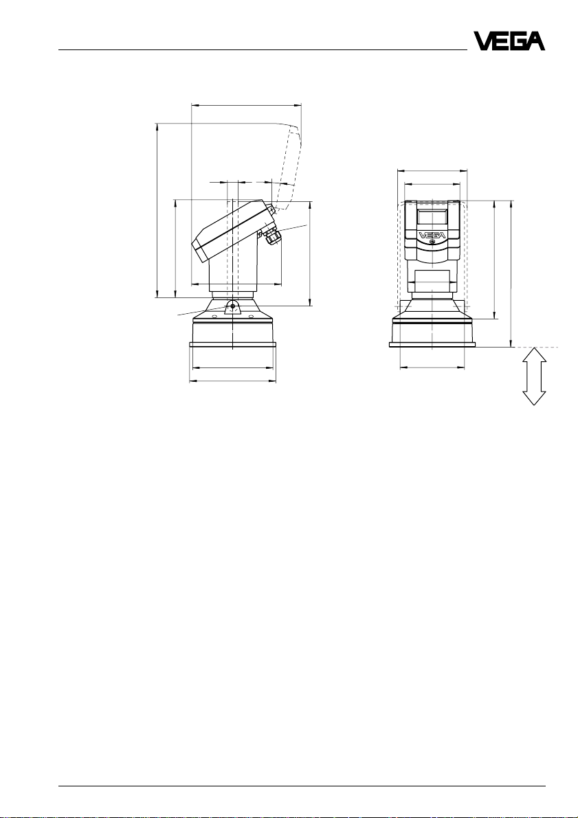
3.2 Dimensions

VEGASCAN 850

260235

246

13 90

210

236

VEGASCAN 850 25

External indicating instrument VEGADIS 50

Technical data

ø5

Pg 13,5

Mounting on carrier rail 35 x 7 .5 acc. to EN 50 022 or flat screwed

135

118

108

Adjustment module MINICOM

Tank 1 m (d)

12.345

67,5

ESC

32,5

Adjustment module for insertion into VEGASON series 50 sensor or into the external indicating instrument VEGADIS 50

Note:

The diameter of the connection cable must be 5 … 9 mm. Otherwise the seal effect of the cable entry will not be ensured.

26 VEGASCAN 850

Technical data

VEGASON 51

Housing PBT

201

Housing aluminium

370

322

182

215

185

10˚

165

M20x1,5

SW 60

G 1½ A/ 1½" NPT

101

116

ø 40

Min. distance to the medium

228

315

Reference plane

0,25 m

205

M20x1,5

SW 60

102

252

337

G 1½ A/ 1½" NPT

Reference plane

ø 40

Min. distance to the medium

0,25 m

VEGASCAN 850 27

VEGASON 52

Housing PBT

Technical data

201

Housing aluminium

370

322

182

215

185

10˚

165

M20x1,5

SW 60

G 2 A

101

116

232

ø 50

Min. distance to the medium

315

Reference plane

0,4 m

205

M20x1,5

SW 60

102

256

337

G 2 A

Reference plane

ø 50

Min. distance to the medium

0,25 m

28 VEGASCAN 850

Technical data

VEGASON 53

201

322

M8x10 12 tief

182

ø 148 ø 158

10˚

165

M20x1,5

195

130

101

118

218

Min. distance to the medium

270

0,6 m

VEGASCAN 850 29

VEGASON 54 … 56 in version A

201

165

Plastic housing (PBT)

10˚

101

Aluminium housing (Al)

116

Technical data

215

185

VEGASON 54

VEGASON 55

397

257

Min. distance to the medium

1,0 m

0,8 m

12xø22

ø190 (ø196)

ø340

ø244 ø405

110 (126)

12xø26

128

12xø22 (12xø26)

445,8

282

Reference plane

VEGASON 56

423

Min. distance to the medium

1,8 m

30 VEGASCAN 850

ø198

ø340 (ø405)

Technical data

VEGASON 54 … 56 in version B

486

4xø19

172

386

245

ø165

ø122,8

201

165

10˚

Plug connection

ø 27

> ø200

Plastic housing (PBT)

11,5

101

503

4xø19

ø165

ø122,8

>ø250

435

270

215

185

Plug connection

798

Aluminium housing (Al)

116

ø165

ø122,8

4xø19

>ø210

ø190 (ø196)

VEGASON 54

1,0 m

Reference plane

189,5

ø 244

VEGASON 55

484,5

0,8 m

ø 198

1,4 m

VEGASON 56

VEGASCAN 850 31

VEGASON 54 … 56 in V ersion C

Aluminium housing (Al)

Plug

Technical data

215

116

185

Plug connection

ø 45

130 150

ø 7

170

445,8

282

10120

1,0 m

0,8 m

VEGASON 54

VEGASON 55

1,4 m

Reference plane

VEGASON 56

32 VEGASCAN 850

Technical data

VEGASON 54 … 56 in version D

Plug connection

3240

214

149

Plastic housing (PBT)

Plug

ø 45

233

3240

167,5

186

101

130 150

201

165

10˚

397,2

257,2

ø 7

120 10

170

3240

527

462,5

Reference plane

1,0 m

0,8 m

1,4 m

VEGASON 54 VEGASON 55 VEGASON 56

VEGASCAN 850 33

4 Mounting and installation

4.1 Mounting VEGASON 54 … 56

Mounting and installation

VEGASON 54 … 56, version A

Sensors in version A (flange version) are supplied completely mounted and ready for operation. Immediately after mounting on the vessel and electrical connection, they are ready for operation.

VEGASON 54 … 56, version B

The sensors in version B are supplied in two parts (transducer and sensor electronics). First of all, mount the transducer on the vessel or above the medium. There is a four-pole jack at the end of the transducer tube. The respective counterpart to the jack protrudes out of the lower side of the sensor electronics housing. Insert the plug of the sensor electronics (only possible in one position) into the jack of the transducer tube. Continue pushing the electronics housing onto the transducer tube, on which there is a wide and a narrow groove.

Groove for locking the headless screw

Mounting groove (must no longer be visible after mounting)

The wide groove is used for locking the headless screws. The narrow groove is a marking for mounting. Move the electronics housing farther down over the transducer tube until the mounting groove is no longer visible. Fasten the housing with the headless screws to the transducer tube. Use a 5 mm hexagon screwdriver (or Allen wrench).

34 VEGASCAN 850

Mounting and installation

VEGASON 54 … 56, version C, D

The sensors in version C and D are supplied in three parts (transducer, sensor electronics and transducer cable). First mount the transducer (see version B). There is a four-pole jack at the transducer tube end. A respective counterpart to the jack is provided in the connection cylinder of the transducer cable. Insert the connection cylinder plug into the jack of the transducer tube.

Connection cylinder

Mounting bracket

Connection cylinder

Transducer cable

On the end of the transducer tube you find a wide and a narrow groove. The wide groove is used for locking the cylinder with the headless screws. The narrow groove is the mounting mark.

Then push the connection cylinder over the transducer tube (with a slight swivelling motion) until the mounting mark is no longer visible.

When the mounting mark is covered by the cylinder, fasten the cylinder with the two headless screws. Use a 5 mm hexagon screwdriver (or Allen wrench).

Now mount the sensor electronics in the requested location. The sensor electronics is fastened to a mounting bracket, so that it can be mounted on a plane surface or on the wall. Make sure that the sensor housing is mounted in such a way that there is enough space above the housing to open the cover.

Now insert the plug at the other end of the transducer cable into the jack on the electronics housing.

Note:

Avoid bending the transducer cable too sharply when laying it out. This is a special cable which could otherwise be damaged.

In addition, make sure that the cable is not damaged during operation. A signal with a voltage of approx. 1 kV is transmitted (which could be a danger in Ex areas if the cable is damaged).

Groove for locking the headless screws

Mounting groove (must no longer be visible after mounting)

VEGASCAN 850 35

Mounting and installation

4.2 General installation instructions

transducer end. For VEGASON 54 ... 56 in version A the lower flange side on the sensor

Measuring range

Beside other criteria, you select your instrument according to the required measuring range. The reference planes for the min. and

is the reference plane. Please note the information on the reference planes in chapter "3.2 Dimensions“. The max. filling depends on the required min. distance and the mounting location.

max. distance to the product or solid is the

VEGASON 51

Min. distance

0.25 m 0.4 m

Full

Empty

max. meas. range

4 m (type 51), 7 m (type 52), 15 m (type 53)

Min. distance, max. measuring range and span (VEGASON 51 … 53)

VEGASON 53 VEGASON 52

Min. distance

0.75 m

Span

Reference plane

Min. distance

VEGASON 56 Version B

Reference plane

min. meas. distance 1.4 m

100 %

0 %

Span

0 %

100 %

Span

VEGASON 54 Version A

min. meas. distance 1.0 m

VEGASON 55 Version B

Reference plane

min. meas. distance 0.8 m

100 %

0 %

max. meas. range

Span

max. meas. distance 25 m (type 54), 45 m (type 55), 70 m (type 56)

Min. distance, max. measuring range, span and reference plane (VEGASON 54 … 56)

36 VEGASCAN 850

Mounting and installation

0 m

15 m

100 %

50 %

1,2

0,4

3˚

8˚

Beam angle and false echoes

The ultrasonic impulses are focused by the transducer. The impulses leave the transducer in conical form similar to the beam pattern of a spotlight.

Any object inside this emission cone will cause a false echo. Especially within the first few meters of the emission cone, pipes, struts, or other installations can interfere with the measurement. At a distance of 6 m, the false echo of a strut has an amplitude nine times greater than at a distance of 18 m.

At greater distances, the energy of the ultrasonic impulses distributes over a large area, thus causing weaker echoes from obstructing surfaces. The interfering signals are therefore less critical than those at close range.

If possible, orient the sensor axis perpendicularly to the product surface and avoid vessel installations (e.g. pipes and struts) within the 100 % area of the emission cone.

The illustrations showing the ultrasonic emission cones are much simplified and represent only the main beam. However, several weaker beams also exist. The transducer must therefore be aligned - especially under difficult measuring conditions - in such a way that very low false echo values result. Putting emphasis only on a strong useful echo is not sufficient under adverse conditions.

Meas. distance

0 m

Meas. distance

7 m

Meas. distance

0 m

4 m

0,4

0,8

0,4

1,2

VEGASON 51

50 % 100 %

5,5˚

0,4

0,8

VEGASON 52

5,5˚

100 %

0,4

1,2

VEGASON 53

emitted power emitted power

12˚

emitted power

50 %

emitted power

Under difficult measurement conditions, we recommend looking for a mounting location with the weakest possible false echoes. The useful echo will then often appear automatically with sufficient quality. With the adjustment software VVO on the PC you can have a look at the echo image and optimise the mounting location (see chapter "6.2 Adjustment with the PC – Sensor optimisation – Echo curve“).

VEGASCAN 850 37

0 m

Meas. distance

Mounting and installation

VEGASON 56VEGASON 54

0 m

emitted power

50 %

100 %

4˚

emitted power

25 m

Meas. distance

45 m

0 m

0,9

2,0

5˚

10˚

242

8˚

0,9

2,0

VEGASON 55

50 %

emitted power

100 %

emitted power

Meas. distance

70 m

50 %

emitted power

6˚

100 %

emitted power

12˚

3,7

7,5

3,7

7,5

38 VEGASCAN 850

Mounting and installation

4.3 Measurement of liquids

Flat vessel top

On flat vessels, the mounting is usually done on a very short DIN socket piece. Reference plane is the lower edge of the flange. The transducer should protrude out of the flange tube.

Reference plane

£ 60 mm

VEGASON 53 on very short DIN socket piece

< 100 mm

Min. distance

Reference plane

< 400 mm

Min. distance

1.8 m

VEGASON 56 in flange version on short DIN socket piece

A mounting location directly on the vessel top is ideal. A round opening in the vessel top is sufficient to fasten the sensor with the flange, or version B and C (VEGASON 54 … 56) with swivelling holder.

Reference plane

Min. distance Type 54: 1 m Type 55: 0.8 m

VEGASON 55 in flange version on short DIN socket piece

VEGASON 53 (compression flange) on flat vessel top

VEGASCAN 850 39

Reference plane

Swivelling holder

Reference plane

Mounting and installation

< 60 mm

Reference plane

Mounting of the transducer with 1“ thread (here belonging to VEGASON 54 version D)

Min. meas. distance

1.8 m

Min. meas. distance

1.4 m

Flange version and swivelling holder on flat vessel top

It is also possible to mount the sensors with 11/2“ or 2“ thread to short socket pieces.

£ 60 mm

Reference plane

Mounting on short 11/2“ or 2“ socket pieces (VEGASON 51)

VEGASON 54 … 56 sensors in version C are mounted in a 1“ thread.

Dished tank ceiling

On dished tank ceilings, please do not mount the instrument in the centre, but approx. 1/ vessel radius from the centre. Dished tank ceilings can act as paraboloidal reflectors. If the transducer is placed at the focal point of the parabolic ceiling, the transducer receives amplified false echoes. The transducer should be mounted outside the focal point. Amplified echoes caused by parabolic surfaces are thereby avoided.

£ 60 mm

VEGASON 51, 52 on dished tank ceiling

Reference plane

/2 vessel radius

40 VEGASCAN 850

Mounting and installation

£ 60 mm

/2 vessel radius

VEGASON 53 on dished tank ceiling

< 400 mm

/2 vessel radius

Reference plane

< 100 mm

/2 vessel radius

VEGASON 54 version A on dished tank ceiling; the statements are also valid for VEGASON 55

Open vessels

On open vessels, use of instruments on an extended mounting bracket is recommended. Mount the low-weight sensor onto such a bracket and ensure a sufficient distance to the vessel wall.

Reference plane

Min. meas.

Reference plane

distance

VEGASON 56 version A on dished tank ceiling

Min. meas. distance

VEGASON 54 on open vessel

VEGASCAN 850 41

Mounting and installation

Pump shaft

Narrow shafts and shaft-like openings (vessel openings) with very rough walls and shoulders make an ultrasonic measurement extremely difficult due to strong false echoes. This problem can be overcome by using an extended socket piece or a complete measuring tube (see chapter "4.5 Socket extension“).

see “4.5 Socket extension“

Socket piece

≥ 250 mm

min. distance

Meas. range

4.4 Measurement of solids

Flange mounting

As with applications for liquids, the instrument can be mounted on a short DIN socket connection on vessels for solids. The transducer axis, however, should point to the vessel outlet or should be oriented perpendicularly to the product surface. The socket length can be max. 60 … 400 mm, depending on the sensor type.

Reference plane

Min. distance

Shaft pump

Measuring tube

Example of a socket extension or measuring tube in a shaft

Shaft pump

VEGASON 53 on inclined vessel flange

Shaft

Very good measuring results can be attained with a measuring tube in continuous narrow shafts, see figure. The applied measuring tube must have smooth walls inside (e.g. PE sewage pipe) and a diameter of 100 mm. This arrangement works well as long as the inside of the measuring tube collects no dirt or buildup (cleaning necessary). You might want to consider using hydrostatic pressure transmitters or capacitive measuring probes. Either the measuring tube should never be immersed in the medium, or it must always

Swivelling holder

We offer as an accessory a swivelling holder (mounting strap) for mounting of VEGASON

53. This simplifies the alignment of the sensor to the product surface.

Suitable is the use of VEGASON 54 … 56 version B or C. For solids, the swivelling holder enables an optimum alignment of the transducer, thus minimising false echoes.

be immersed (so that the measurement is carried out exclusively in the tube).

42 VEGASCAN 850

Mounting and installation

Reference plane

Min. distance

Mounting boss

Reference plane

Min. distance

VEGASON 53 on swivelling holder

Reference plane

Min. distance

VEGASON 54C with adapter flange and swivelling holder on a DN 200 vessel flange

VEGASON 51 or 52 on the mounting boss. The socket axis should point directly to the product surface. This is why VEGASON 51 and 52 are less suitable for solids.

Reference plane

Min. distance

VEGASON 56 in 1“ mounting boss.

The socket axis should point directly to the product surface. Much better would be the use of a swivelling holder version.

VEGASCAN 850 43

Mounting and installation

Material heaps

Large material heaps are best detected with several instruments, which can be mounted on e.g. traverse cranes. For this type of application, it is advantageous to orient the sensor directly toward the solid surface.

Transducer on traverse crane above a material heap (illustration: VEGASON 54 in version B)

4.5 Socket extensions

The ultrasonic sensors require a min. distance to the liquid or solid product. Take the min. distance into account in your planning. In some situations, it is possible to reach the required min. distance, and hence the desired filling height, with a socket extension. However, the socket extension increases the noise level of the ultrasonic signal at the extension outlet and can interfere with the measurement. Only use a socket extension if all other possibilities have to be excluded. Carry out the extension as shown in the following illustration.

Socket extensions in liquids

Chamfer and deburr the socket carefully and make sure it has a smooth inner surface. The socket should not protrude into the measured product, in case buildup can form on the socket through pollution or product residues.

Socket piece should not be immersed into adhesive products (illustration: VEGASON 53)

The socket diameter should be as large and the socket length as small as possible. Make sure that the socket outlet is burr-free to minimise false echoes.

44 VEGASCAN 850

Mounting and installation

15˚ 15˚

Type 51/52

45˚

Socket extensions in liquids

Type 53

45˚

Max. socket length in relation to socket diameter

ø in mm L in mm

Type 51 Type 52 Type 53

100 200 300 300 150 300 400 400 200 – 500 500 250 ––600

Type 54

Type 55

Socket extensions for solids

For solids, use a conical socket extension with a taper of at least 15° … 20°.

Socket extension in solids

Measurement in a tube

For nonadhesive measured products, a socket extension in the form of a measuring tube can be permanently submerged in the product. The ultrasonic measurement is then made exclusively in the measuring tube and works very well without interference from other vessel installations (see "Pump shaft“).

45˚

Socket extensions that do not protrude into the measured product

45˚

Max. socket length in relation to socket diameter

ø in mm L in mm

Type 54 Type 55 Type 56

200 400 –– –– 250 500 500 500 300 –– –– 600

VEGASCAN 850 45

Mounting and installation

4.6 Flow measurement

The short examples on this page are only basic information on flow measurement. You can get complete planning information from the flume manufacturers and in special literature.

Rectangular flume

- Installation of the sensor on the upstream side

- Note distance to the overfall edge (3 … 4 x h

- Installation centered to the flume

- Edge opening ³ 2 x h

- Installation perpendicular to the liquid surface

- Keep min. distance in relation to h

- Min. distance from edge opening to downstream water ³ 50 mm

max

90°

)

from ground

max

³ max. distance

max

Khafagi-Venturi flume

- Installation of the sensor on the inlet side

- Note distance to the Khafagi-Venturi flume (3 … 4 x h

- Installation perpendicular to the liquid surface

- Keep min. distance in relation to the height of damming h

Khafagi-Venturi flume

max

3 … 4 x h

90°

Sensor

)

max

³ 2 x h

Overfall edge

max

Flow measurement on open flumes

Overfall edge

3 … 4 x h

max

90°

³ 5 cm

Upstream water

Downstream water

Flow measurement on open flumes

46 VEGASCAN 850

Mounting and installation

4.7 False echoes

The mounting location of the ultrasonic sensor must be selected such that no installations or inflowing material are in the path of the ultrasonic impulses. The following examples and instructions show the most frequent measuring problems and how to avoid them.

Vessel protrusions

Vessel forms with flat protrusions can, due to their strong false echoes, adversely effect the measurement. Shields above these flat protrusions scatter the false echoes and guarantee a reliable measurement.

Correct Wrong

Vessel protrusions (slope)

Intake pipes, e.g. for the mixing of materials with a flat surface directed towards the sensor - should be covered with a sloping shield. This shield will scatter false echoes.

Vessel installations

Vessel installations such as, for example, a ladder, often cause false echoes. Make sure when planning your measurement loop that the ultrasonic signals have free access to the measured product.

Correct Wrong

Ladder

Vessel installations

Ladder

Struts

Struts, like other vessel installations, can cause strong false echoes that are superimposed over the useful echo signals. Small shields effectively hinder a direct false echo reflection. These false echoes are scattered and diffused in the area and are then filtered out as "echo noise“ by the measuring electronics.

Correct Wrong

Shields

Struts

Vessel protrusions (intake pipe)

VEGASCAN 850 47

Mounting and installation

Inflowing material

Do not mount the instrument in or above the filling stream. Ensure that you detect the product surface and not the inflowing material.

Correct

Wrong

Correct

Buildup

Wrong

Overflow basin

The expected max. high water determines the installation height, to ensure the min. distance of the transducer even with the highest water level. The low water level should be covered in the transducer area with a shield to filter out echoes from exposed basin surfaces.

Correct Wrong

Inflowing material

Min. distance high water

Buildup

If the sensor is mounted too close to the vessel wall, buildup and adhesions of the measured product to the vessel wall can cause false echoes. Position the sensor at a sufficient distance from the vessel wall. Please also note chapter "4.2 General installation instructions“.

48 VEGASCAN 850

60°

Shield

Filtering out of a level echo

Low water

Mounting and installation

Strong product movements

Heavy turbulences in the vessel, e.g. by strong stirrers or strong chemical reactions, can seriously interfere with the measurement. A surge or bypass tube of sufficient size (DN 200, DN 250) always allows, provided the product causes no buildup in the tube, a reliable measurement even with strong turbulences in the vessel.

100 %

60 %

0 %

Strong product movements

4.8 Incorrect mounting

Foam generation

Thick foam on the product can cause incorrect measurements. Take measures to avoid foam, carry out the measurement in a bypass tube, or use a different measuring technology, e.g. capacitive measuring probes or hydrostatic pressure transmitters.

Foam generation

Wrong orientation to the product

Weak measuring signals are the result if the sensor is not directly pointed at the product surface. Orient the sensor axis perpendicularly to the product surface to achieve optimum measuring results.

Orient the sensor perpendicularly to the product surface

VEGASCAN 850 49

Mounting and installation

Strong heat fluctuations

Strong heat fluctuations, e.g. due to the sun, cause measuring errors. Please provide a sun shield.

Shield

Strong heat fluctuations

Min. distance to the medium

If the min. distance to the medium is not maintained, the instruments show wrong measured values. Mount the instrument at the required min. distance.

Sensor too close to the vessel wall

If the sensor is mounted too close to the vessel wall (dimension A in diagram), strong false echoes can be caused. Buildup, rivets, screws or weld joints on the vessel wall superimpose their echoes onto the product or useful echo. Please ensure a sufficient distance from the sensor to the vessel wall, depending on the maximum measuring distance (dimension B in diagram).

In case of good reflection conditions (liquids, no vessel installations), we recommend determining the sensor distance according to Diagram curve 1. At a max. meas. distance of e.g. 10 m, the distance of the transducer (according to curve 1) should be approx.

1.5 m.

In case of solids with bad reflection properties, determine the distance to the vessel wall according to Diagram curve 2. Under very bad measuring conditions (rough vessel walls, struts), it might be necessary to increase the distance to the vessel wall, or to additionally filter out the false echoes by storing them in memory, thereby adapting the sensor more precisely to the environment.

Correct Wrong

Sensor too close to the vessel wall

50 VEGASCAN 850

Mounting and installation

Distance of the transducer to the vessel wall

1 m 2 m 3 m 4 m 5 m

Curve 1 (liquids)

5 m

10 m

15 m

max. meas. distance

Curve 2 (solids)

Distance from the sensor to the vessel wall, depending on the meas. distance (type 51 … 53)

Distance of the transducer to the vessel wall

Parabolic effects of rounded or arched vessel tops

Round or parabolic tank tops act on the signals like a parabolic mirror. If the sensor is placed at the focal point of such a parabolic tank top, the sensor receives amplified false echoes. The optimum location is generally in the area of half the vessel radius from the centre.

Correct

< 100 mm

~ 1/

vessel radius

Wrong

2 m 4 m 6 m 8 m

Wrong

Curve 1 (liquids)

10 m

20 m

Curve 2 (solids)

Mounting on a vessel with parabolic tank top

30 m

max. meas. distance

Distance from the sensor to the vessel wall, depending on the meas. distance (type 54 … 56)

VEGASCAN 850 51

Socket piece too long

If the sensor is mounted in a socket extension that is too long, strong false echoes are caused, and measurement is hindered. Make sure that the transducer protrudes at least 30 mm out of the socket piece.

Reference plane

< 100 mm

Mounting and installation

Correct and wrong length of socket piece

52 VEGASCAN 850

Electrical connection

5 Electrical connection

5.1 Connection, connection cable and shielding

Qualified personnel

Instruments which are not operated with protective low voltage or DC voltage must only be connected by qualified personnel. This is especially valid for the connection of the power supply on VEGASCAN.

Safety information

As a rule, do the work in the complete absence of voltage. Always switch off the power supply before you carry out connecting work. Protect yourself and the instruments.

The shielded transducer cables transmit a signal with a voltage of approx. 1 kV. In Ex areas, cable damage can be dangerous. Do not carry out any mounting or connection work on the transducer when VEGASCAN is switched on.

Connection cable

Please note that the connection cables are specified for the expected operating temperatures in your systems. The power supply and the sensor cables must have an outer diameter of 6 … 12 mm, to ensure the seal effect of the cable entry.

Transducer cable

When wiring the transducer cable (version C and D), strong bending of the cable should be avoided. This is a special cable which can be damaged.

Make sure when wiring the transducer cable that no operating influences can damage it.

Earth conductor terminal

The electronics housing of the sensors has a protective insulation. The earth conductor terminal and the earth terminal in the electronics housing are galvanically connected with the metallic transducer diaphragm. On sensors in version B, the earth conductor terminal is galvanically connected to the transducer diaphragm via the transducer tube when the sensor is completely mounted. On version C and D, the connection is made via the cable screen of the transducer cable and the transducer tube.

Shielding of the sensor cables

The "Electromagnetic pollution“ from electronic actuators, power lines and transmitting stations is often so considerable that the twowire cable of VEGASCAN to the sensors must be shielded.

Power supply

For power supply, standard three-wire cable up to max. 2.5 mm2 can be used. The electrical connection is made via spring terminals. You open the terminal opening with a small screwdriver by inserting it into the opening slot above the terminal position and lever it upward. This opens the terminal and the copper core of the connection wire can be inserted.

VEGASCAN 850 53

Electrical connection

We recommend a screening on both ends, see the following sketch. Screening is a good preventative measure against future sources of interference. However, you must make sure that no ground potential currents flow through the sensor cable shields. Ground potential currents can be avoided by potential equalisation cables. When grounding at both ends, it is possible to connect the cable

Note Ex protection!

In Ex applications, grounding on both ends is not allowed due to potential losses. If an instrument is used in hazardous areas, the respective regulations, conformity certificates and type approvals for systems in Ex areas must be noted (e.g. DIN 0165). Please note the approval documents with the

safety data sheet attached to the Ex sensors. shield on one side (e.g. in the switching cabinet) via a capacitor (e.g. 0.1 µF; 250 V) to the ground potential. Use a low-resistance ground connection (foundation, plate or mains earth).

Linear (serial) arrangement of sensors

Grounding of the cable screen on both ends, at the end of each sensor line via a ground capacitor.

850

54 VEGASCAN 850

Electrical connection

Radial arrangement of sensors

Grounding on at least two ends, on VEGASCAN and once on the sensor star, i.e. on the longest sensor line. If the individual sensor lines are longer than approx. 15 m, a grounding of each longer line should be made via a ground capacitor.

850

Longest stub of the sensor star

VEGASCAN 850 55

Electrical connection

5.2 Connection of the sensor

After mounting the sensor at the measurement location according to the instructions in chapter "4 Mounting and installation“, loosen the closing screw on top of the sensor. The sensor lid with the optional indication display can then be opened. Unscrew the sleeve nut and slip it over the connection cable (after removing about 10 cm of insulation). The sleeve nut of the cable entry has a self-locking ratchet that prevents it from opening on its own.

Version with aluminium housing

Voltage supply and digital meas. signal

M20 x 1.5 (diameter of the connection cable 6…9 mm)

To the indicating instrument in the cover or to the external indicating instrument VEGADIS 50

M20 x 1.5

Now insert the cable through the cable entry

into the sensor. Screw the sleeve nut back

onto the cable entry and clamp the stripped

wires of the cable into the proper terminal

positions.

The spring terminals hold the wire without a

screw. Press the white opening tabs with a

small screwdriver and insert the copper core

of the connection cable into the terminal

opening. Check the hold of the individual

wires in the terminals by lightly pulling on

them.

Version with plastic housing

Voltage supply and digital meas. signal

To the indicating instrument in

Cable entry M20 x 1.5

the cover or to the external indicating instrument

Sockets for connection of VEGACONNECT 2 (communication sockets)

12 C 567843

12 C 5 6 7 8

(+) (-)

Communication

Display

ESC

VBUS

Terminals (max. 2.5 mm wire cross-section)

Sockets for connection of the HART handheld or VEGACONNECT

pluggable adjustment module MINICOM

12 C 5678

Commu-

(+) (-)

nication

VBUS

Tank 1 m (d)

12.345

Display

ESC

Opening tabs

56 VEGASCAN 850

Electrical connection

5.3 Connection of the external indicating instrument VEGADIS 50

Loosen the four screws of the housing cover on VEGADIS 50. The connection procedure can be facilitated by fixing the housing cover during connection work with one or two screws on the right of the housing (figure).

OUTPUT (to the sensor)

Adjustment module

VEGADIS 50

Tank 1 m (d)

12.345

ESC

Voltage supply and digital meas. signal

12 C 5678

(+) (-)

VBUS

Tank 1 m (d)

12.345

C 5678

Commu nication

Display

ESC

DISPLAY

(in the cover of the indicating instrument)

Screws

VEGASCAN 850 57

Electrical connection

5.4 Connection of the sensors to

VEGASCAN 850

off

---

POWER

GNDTxD

RxDDTR

FIELDBUS VBUS1 VBUS2

PC2

PE L

VBUS1

Use the terminal VBUS1, when using a VEGASCAN 850 for 15 sensors. Sensors 16 … 30 are connected to the terminals VBUS2.

+++

--+++

VBUS2

The electrical connection is made by spring

terminals. The clamping opening can be

opened with a small screwdriver by inserting

it into the opening slot above the clamping

position and pushing upwards. Then the

terminal and the copper core of the connec-

tion wire can be inserted.

Up to 15 sensors can be connected to each VBUS branch on one two-wire cable.

---

+++

Sensor 1 … 15

VBUS1

It is a good idea to optimise the current distribution by dividing the BUS into three branches with five sensors each.

Sensor

Sensor 6 … 10

Sensor 11 … 15

1 … 5

---

+++

VBUS1

58 VEGASCAN 850

Electrical connection

5.5 Signal output/Interface connection

The connection terminal is labelled for the field bus cable according to the selected interface and instrument version.

Modbus, VEGA-ASCII, Siemens 3964

TXRX

DATA

(B/B´)

DATA

(B/B´)

Interface RS 232

/TX/RX

Interface RS 422

Interface RS 485

DATA

(A/A´)

Interface RS TTY

Interface RS 485

DATA

(A/A´)

RxD

GND TxD

FIELDBUS

GND

FIELDBUS

GND

(C/C´)

FIELDBUS

T-

R+ R+

GND T+

FIELDBUS

Profibus DP , Profibus FMS

GND

(C/C´)

FIELDBUS

5.6 Connection of the PC to VEGASCAN 850

The PC with the adjustment software VVO can be connected in the front panel or in the terminal compartment of VEGASCAN.

For connection of the PC in the front panel (9pole socket) you require a standard RS 232 DTE-DTE (Data Terminal Equipment) interface cable.

DCD

RxD

TxD

DTR

GND

...

For connection of the PC in the terminal compartment, connect the opened PC cable according to the following sketches to terminal block PC2. For communication, only three wires of the 9-pole cable are used.

DCD

RxD

TxD

DTR

GND

...

DCD1

RxD2

TxD3

DTR4

GND5

...

GNDTxD

RxD DTR

PC2

Terminal in VEGASCAN

VEGASCAN 850 59

6 Setup

Setup

6.1 Adjustment methods

VEGASCAN 850 and the series 50 ultrasonic sensors are adjusted with the PC (adjustment program VVO). With the detachable adjustment module MINICOM, it is possible to adjust the sensors individually. The adjustment can be carried out with only one adjustment instrument at a time.

With the PC

The PC with the adjustment program VVO (VEGA Visual Operating) can be connected to:

- VEGASCAN 850

- the sensor

- the signal cable

With the adjustment program VVO (VEGA Visual Operating) on the PC you adjust the level measuring system consisting of VEGASCAN and ultrasonic sensors. The PC communicates via the standard RS 232 interface cable with VEGASCAN and all connected sensors. For this purpose, a digital adjustment signal is superimposed on the signal and supply cable.

In the following chapter "6.2 Adjustment with the PC“, the adjustment is described when connecting the PC via a RS 232 interface cable to VEGASCAN. When connecting the PC via VEGACONNECT to the sensor signal cable (see "2.6 Configuration of measuring systems“ configuration A), all sensors connected to the affected signal cable are available for adjustment. However, the configuration and measured data processing functions of VEGASCAN are not available.

When inserting VEGACONNECT into the communication socket of an individual sensor, only sensor-relevant adjustment options such as e.g. sensor optimisation on the affected sensor are adjustable. Other sensors and VEGASCAN are then not adjustable. This is due to an adjustment hierarchy beginning with VEGASCAN and ending with the sensor.

With the adjustment module MINICOM

With the adjustment module MINICOM you adjust the individual sensor directly in the sensor or in the external indicating instrument VEGADIS 50. The adjustment module MINICOM with the 6 key adjustment field with text display enables the parameter adjustment of the sensor with an array of functions comparable to the adjustment program VVO when connected via VEGACONNECT to the sensor, but not the configuration of the measuring system.

Beside the connection of the PC to VEGASCAN, it is possible to connect the PC with the interface converter VEGACONNECT to the signal cable between sensor and VEGASCAN or also directly to the individual sensor.

60 VEGASCAN 850

Setup

6.2 Adjustment with the PC

In the following setup and adjustment instructions you will find information on the following topics and adjustment points:

• Configuration

- configuration info

- create new measurement loop

• Parameter adjustment 1

- adjustment

- scaling

• Sensor optimisation

- meas. environment

- sound velocity

- echo curve

- false echo storage

• Parameter adjustment 2 (optional)

- linearisation

- parameter adjustment sensor display

- meas. loop data

• Display of measured value

• Simulation

• Select available linearisation curve

• Print configuration and adjustments

• Backup

Note:

Keep in mind that you first have to log in a sensor in the configuration menu before you can continue with the parameter setting, and if necessary, carry out adjustments in the menu “Sensor optimisation”.

For connection of the PC to VEGASCAN, a standard RS 232- DTE-DTE (Data Terminal equipment) interface cable is required. With the cable, the PC is connected to VEGASCAN.

DTE DTE

Beside the measured values, the adjustments signals are also transmitted digitally via the signal supply cable between sensor and VEGASCAN. The adjustment program VVO can then communicate with VEGASCAN and all connected sensors. In chapter "2.6 Configuration of measuring systems“ the connection of the PC to the different sensor arrangements is shown.

Before starting the setup:

Do not be confused by the many pictures, adjustment steps and menus on the following pages. Just carry out the setup with the PC step-by-step and you will soon no longer need the following pages. Whenever you should adjust or choose something, this is indicated in the following by a large black dot, like this:

• Choose …

• Start …

• Click to …

• Connect the standard output of your PC by

the standard RS 232 interlink cable (9pole) to VEGASCAN.

• Now switch on the power supply of the

processing system.

By this means, the actions to be carried out are clearly separated from supplementary information in the following adjustment instructions.

Approx. 1 … 2 minutes after switching on the supply voltage, the sensors generally show measured values on the sensor display.

After the adjustment software on the PC has attained connection to VEGASCAN, you start with the "Configuration“ of your measuring system.

DCD 1 1 DCD RxD 2 2 RxD TxD 3 3 TxD DTR 4 4 DTR GND 5 5 GND

--- 6 6 ---

--- 7 7 ---

--- 8 8 ---

--- 9 9 ---

VEGASCAN 850 61

• First start the adjustment software VVO on your PC.

• Choose with the arrow keys or the mouse the item "

Planning

“ on the entrance screen

and click to "OK“.

In the next window you are asked for the user identification.

Setup - Adjustment with the PC

If the VVO (adjustment software) gets in contact with VEGASCAN for the first time, you are asked if you want to transfer the data from VEGASCAN to the PC.

• Enter under name "VEGA.

• Also enter "VEGA under password.

The adjustment program VEGA Visual Operating (VVO), called in the following VVO, gets into contact with VEGASCAN and the sensors …

… and asks in which mode you want to use the adjustment software. After a few seconds the software indicates if and with which sensor a connection exists.

• Click to "

YES

“.

If you want to connect the VVO to a VEGASCAN, to which in the meantime another PC was connected, you will be asked, if you want to transfer the saved data from the actual PC to VEGASCAN or the data of VEGASCAN to the PC.

When clicking to "

Quit

“, you are immediately in the main menu window of the adjustment software VVO.

The preset user identification can be modified later in the menu "

User access

Configuration/Program/

“.

62 VEGASCAN 850

Setup - Adjustment with the PC

Note:

If you get no sensor connection, check the following:

- Is the sensor being supplied with voltage from VEGASCAN (min. 17 V)?

- Are you using the correct interface cable?

- Is the RS 232 cable connected to the correct COM-Port?

Change COM-Port

In the menu "

nication

eters of your PC or change the activated COM-Port.

Configuration/Program/Commu-

“ you can adjust the interface param-

Configuration

During the setup of VEGASCAN you are confronted with two terms: "Configuration“ and "Parameter adjustment“. The meas. system VEGASCAN is first set up with a configuration and then with a parameter adjustment.

Configuration

The term "Configuration“ means the basic adjustments of VEGASCAN. You inform VEGASCAN about the application (level measurement, gauge, distance …), the measurement loop name and the DCS output address of the sensors. The configuration corresponds to an electronic wiring and labelling of your VEGASCAN or just which sensor for what application and where.

Parameter adjustment

After the configuration, you carry out the parameter adjustment for each individual sensor. This means, to adjust the sensors to the respective operating range and to adjust to the actual application. You inform the sensor which product distance (which level) is "empty“ and which "full“. This is called adjustment. Here you choose in which physical unit (volume, mass) and unit of measurement (m3, gal, liters …) the adjusted measured value should be outputted. In the submenu "Sensor optimisation“ you inform the sensor electronics about the actual environment, such as e.g. quick changes of the measured value, foam generation, gas stratification, solid or liquid.

VEGASCAN 850 63

Setup - Adjustment with the PC

Configuration info

• Choose the menu "Configuration/Measur-

ing system.

You reach the menu window "

measuring system

“. Here you get all informa-

Configuration

tion on the connected VEGASCAN.

User authorisation

• Save your password with "

Save

“ and you are again in the initial menu of the configuration.

Communication

• Click in the menu window "

measuring system

Configuration

“ to "

Communication

“.

Unauthorised access to VEGASCAN can be prevented by a password. For each connection location of the PC, on the D-SUB plug in the front of VEGASCAN (PC) or fixed connection in the terminal compartment (PC2), a respective password can be allocated.

• Click to "

64 VEGASCAN 850

Access protection activated“.

Here you adjust the interface parameters for your signal output (here Modbus).

• Click to " with "

• Click to "

Quit

Save

“ or quit the menu window

“.

VBUS1

“.

Setup - Adjustment with the PC

You get an overview of the sensors connected to the VBUS1 terminal position and their configuration status.

If a sensor was logged in as described in the following menu " status "

Configure

overview.

Create new measurement loop

• Choose the menu "Configuration/Measure-

ment loop/New

• In the menu window "

ment loop tion

“ with "OK“.

Measurement loop/New

“ is written in the sensor

“.

“, you choose "

Create new measure-

a new applica-

“, the

You are in the menu window "

measurement loop - Application

• Choose the parameter "

ment

“ and the sensor type "

• Click to "

• Choose in the next menu window "

ard level measurement

• Click to "

After a few seconds, the menu window "

Continue

“.

Create new

“.

Level measure-

Ultrasonic

“ and "

Stand-

no options

“.

Create new measurement loop - Sensor configuration

“ opens.

• Click to "

The small menu window "

tion

VEGASCAN 850 65

Sensor coordination

“ opens.

“.

Sensor coordina-

Setup - Adjustment with the PC

• Choose the serial number of the sensor to be assigned and confirm with "OK“.

In the menu window "

ment loop - Sensor configuration

number and the serial number of the sensor are displayed instead of "not configured“.

• Now click in the menu window "

Create new measure-

“, the VBUS

-Create new

measurement loop - Sensor configuration

to "

Continue

• Click in the menu window "

“.

Create new measurement loop - Measurement loop designation

“ to "

Level

“.

The menu window "

Create new measurement

loop - Measurement loop designation

Enter here the measurement loop number and a measurement loop description.

• Assign here also one or several PC/DCS addresses to the actual sensor by clicking to "

PC/DCS address

“

“.

“ opens.

66 VEGASCAN 850

Setup - Adjustment with the PC

• Confirm the adjustment with "OK“.

• Also here confirm with "OK“ and you are

again in the initial window "

Create new measurement loop - Measurement loop designation

“, in which the measurement loop number and the previously entered measurement loop description are now displayed.

In the menu "

Configuration/Measuring sys-

tem“ you now see the configured sensors.

Now, you only have to carry out the parameter adjustment for the sensor. The parameter adjustment is described in the following under Parameter adjustment 1 and Param-

• Click to "OK“ and you are again in the main menu window.

You have just carried out the configuration

eter adjustment 2. Parameter adjustment 1 is obligatory, whereas parameter adjustment 2 (after sensor optimisation) must only be carried out if necessary.

settings for one sensor on VEGASCAN.

VEGASCAN 850 67

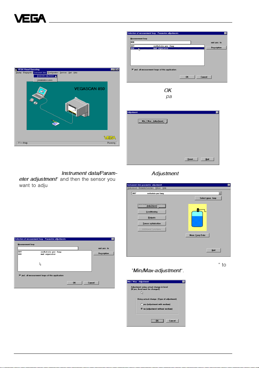
Parameter adjustment 1

Setup - Adjustment with the PC

In the menu "

justment

adjustments.

Adjustment

• Choose the menu "

eter adjustment

want to adjust.

In the opening menu window, you now see the previously entered measurement loop names and the measurement loop descriptions. If you have only configured one sensor, naturally you will have a choice of only one sensor.

Instrument data/Parameter ad-

“ you carry out all important sensor

Instrument data/Param-

“ and then the sensor you

• Then click to "OK“, the menu window "

strument data parameter adjustment

opens.

• Click to "

Adjustment

“.

In-

“

• Click in the menu window "

Min/Max-adjustment

• Click to the sensor or the measurement loop on which you want to carry out the parameter adjustment.

68 VEGASCAN 850

“.

Adjustment

“ to

Setup - Adjustment with the PC

You can carry out the min./max. adjustment

"with medium“

actual level) or taking the actual level into consideration, i.e. with empty vessel).

Generally, you will carry out the adjustment without medium. Then you are not concerned about the actual vessel filling during adjustment. When you want to carry out the adjustment with medium, you have to carry out the min. adjustment with emptied (also partly emptied) vessel and the max. adjustment with filled (also partly filled) vessel. It is convenient and quick to carry out the adjustment without medium, as shown in the example.

• Choose "

• Choose if you want the carry out the ad-

justment in

• Enter a distance for the upper and lower level and the volume in % corresponding to each distance.

In the example, the 0 % filling is at a product distance of 3.400 m and the 100 % filling at a product distance of 0.500 m.

Note:

The instrument is supplied with the operating range identical to the sensor measuring range. After sensor adjustment, the operating range corresponds to the adjustment. The sensor can only detect levels within the defined operating range. For the detection of levels outside the operating range, e.g. new adjustment, it is necessary to correct the operating range in the menu "

sation/Meas. environment

(adjustment by means of the

"without medium“

no (adjustment without medium)

meters

(m) or in

(without

feet

(ft).

Sensor optimi-

“

• Confirm your adjustments with "OK and

you are again in the menu window "

ment

“.

• Click in the menu window "

Quit

“.

You are again in the menu window "

“.

ment data parameter adjustment

Now the sensor electronics has two characteristics points, one for min. and one for max., out of which a linear correlation between product distance and the percentage filling of a vessel is generated. Naturally the characteristics point must not be at 0 % and 100 %, however the distance should be as big as possible (e.g. at 20 % and at 80 %). The difference between the characteristics points for the min./max. adjustment should be at least 20 mm product distance. This is a theoretical value, because if the characteristics points are too close together, the possible measuring error increases. Ideal would be, to carry out the adjustment as shown in the example, at 0 % and at 100 %.

Adjustment

“.

Adjust-

“ to

Instru-

VEGASCAN 850 69

Setup - Adjustment with the PC

In the menu "

justment/Conditioning/Linearisation

enter later, if necessary, a correlation between product distance and percent value of volume other than linear (see later subitem linearisation).

Scaling

• Click in the menu window "

parameter adjustment

The menu window "

Instrument data/Parameter ad-

“ you can

Instrument data

“ to "

Conditioning

“ opens.

“.

As parameter you can choose

less

(plain numbers),

and distance“

measuring unit (e.g. l, hl). The sensor display then shows the measured value in the selected parameter and unit.

• Save the adjustments in the menu " by clicking "OK.

volume, mass, height

and assign an appropriate

"dimension-

Scaling

“

The adjustments are now transferred to the sensor and you are again in the menu window "

Conditioning

• Click in the menu window " "

Quit

“.

• Click to "

In the menu " 0 % and 100 % values of the parameter and their unit. You thereby inform the sensor, e.g. that at 0 % filling there are still 45 liters and at 100 % filling 1200 liters in the vessel. The sensor display then shows with empty vessel (0 %) 45 liters and with full vessel (100 %) 1200 liters.

70 VEGASCAN 850

Scaling

“.

“ you enter the actual

• Click in the menu window "

parameter adjustment

“.

Conditioning

“ to

Instrument data

“ to "

Quit

“.

Setup - Adjustment with the PC

Sensor optimisation

In the menu "Sensor optimisation“ you can adapt the sensor to the environment. Here you carry out special optimising adjustments and optimise, e.g. by means of the echo curve, the mounting location of the sensor.

Meas. environment/Operating range

• Choose the menu "

eter adjustment

• Choose in the menu window "

data parameter adjustment

Sensor optimisation and click to "

“.

• First click to "Meas. environment.

Instrument data param-

“

Instrument

“ the menu item

Sensor

The window "

With the menu item " can define the operating range of the sensor deviating from the measuring range (depending on the sensor type) and the "

Max adjustment

range corresponds otherwise to the min./ max. adjustment (span) or the measuring range.

Generally, it is better to choose the operating range approx. 5 % bigger than the adjusted measuring range (span) determined by the min./max. adjustment. In the example:

- Min. adjustment to 1.270 m,

- Max. adjustment to 5.85 m. In the example you would have adjusted the operating range from 1 m to 6 m.

Meas. environment

“ opens.

Operating range

“. By default, the operating

“ you

Min/

• Save the adjustments and quit the menu window " with "

VEGASCAN 850 71

Limitation of the operating range

Quit

“.

“

Meas. environment/Meas. conditions

Setup - Adjustment with the PC

• Click in the window "

Measuring conditions.

• In the menu window " you click on the options corresponding to your application.

• Confirm with "OK.

After a few seconds of saving during which the adjustments are permanently saved in the sensor, you are again in the window "

Meas. environment

Sonic velocity

When measuring in a gas composition deviating from air, e.g. pure nitrogen, the sonic velocity will change. Without correction, this would distort the measuring result.

Meas. environment

Measuring conditions

“.

“ to

• Confirm with "OK“.

• Click in the menu window "

ment

“ to "Quit.

You are again in the menu window "

optimisation

Echo curve

“

If, due to vessel installations, you expect strong false echoes, a correction (if possible) of the mounting location and orientation (during simultaneous monitoring of the echo curve) can help localise the false echoes and reduce their intensity. With the menu item "

Echo curve

optimisation

intensity of the detected ultrasonic echoes.

“.

“ in the menu window " “ you can see the form and the

Meas. environ-

Sensor

In the menu " can be adapted to the correct value in case of another gas composition.

72 VEGASCAN 850

Sonic velocity

“ the sonic velocity

Setup - Adjustment with the PC

In the illustration, you see the echo curve (before correction of the sensor orientation) with a false echo nearly as large as the product echo.

In the next illustration you then see the echo curve after optimum directing of the sensor to the product surface and away from a large false echo source (sensor axis perpendicular to the product surface). The false echo, caused e.g. by a strut, is now reduced by more than 30 dB and will no longer influence the measurement.

• Quit the menu "

Echo curve

“ with "Quit.

False echo storage

With the menu item " the menu "

Sensor optimisation

False echo storage

“ you can au-

“ in

thorise the sensor to save false echoes. The sensor electronics then saves the false echoes in an internal database and assigns them a lower level of importance than the useful echo. The false echo storage should be carried out with empty vessel.

• Click in the menu window "

tion

“ to the menu item "False echo storage.

Sensor optimisa-

VEGASCAN 850 73

Setup - Adjustment with the PC

• Now click in the opening menu window "

False echo storage

oes. A small window opens.

• Enter here the verified product distance and click to "Create new

You hereby authorise the sensor to mark all echoes before the product echo as false echoes. This prevents the sensor from erroneously detecting a false echo as level echo.

• Click to "Show echo curve.

“ to "Learn false ech-

.

• Quit the menu with "Quit.

You are again in the menu window "

optimisation

reset all options out of the menu "

optimisation

• Quit the menu window "

tion

Sensor optimisation sensor selection

with "

You are then in the initial menu window "

“. With the menu item "

“ to default.

Sensor optimisa-

“ with "Quit and the menu window

Quit

“.

strument data parameter adjustment

Sensor

Reset

Sensor

“.

“ you

“ also

In-

The curve of the false echo marking and the real echo curve (top) are shown.

74 VEGASCAN 850

Setup - Adjustment with the PC

Parameter adjustment 2

Linearisation

The relation between level and filling volume is described with so-called linearisation curves. If, in your vessel, there is a correlation other than linear between level ("

age value

(value of the filling volume), choose in the menu window " "

Instrument data/Parameter adjustment/Con-

ditioning

“ of the level) and the filling volume

Conditioning

“.

“ the menu item

Percent-

Beside the two programmed linearisation curves "

Horizontal cylindrical tank

Spherical tank

programmable curves

is a linear correlation between level and volume.

User programmable linearisation curves

• Click to "User programmable curve to enter your own vessel geometry or a user programmable filling curve.

• Click to "Edit.

“ you can also enter "

“. Linear means there

“ and

user

• Click in the menu window " the menu item "Linearisation.

The menu window " correlation between percentage value of the level and the percentage value of the filling volume is preadjusted.

VEGASCAN 850 75

Linearisation

Conditioning

“, in which a

“ to

Setup - Adjustment with the PC

The user programmable linearisation curve is generated by index markers. Each index marker consists of one value pair. A value pair is generated out of a value " and a value "

value

the level. "

Percentage value“

“ represents the percentage value of

Linearised

“ represents the per-

Linearised

. "

Percentage

“

centage vessel volume at a certain percentage value of the level.

In the field "

Transfer measured value

“ the current level as percent of the adjusted span is displayed. The measuring span has already been adjusted with the min./max. adjustment. In our example, the measuring span is 4.58 m and is in the range of 5.85 m (empty) up to 1.27 m (full), see the following illustration.

0 m

100 % or 1.27 m

The percentage value of 95.79 % means that now 4.387 m of the adjusted measuring span (4.58 m) are reached:

4.58 • 0.9579 = 4.387 m.

The distance (product distance) outputted by the sensor, in case you have chosen "

distance

“ as output parameter, is then:

5.85 – (4.58 • 0.9579) = 1.463 m.

If the index markers or value pairs of your vessel are not known, you have to define the linearisation curve by incremental filling or calculate it with the vessel calculation program of VVO (see next page).

Defining the linearisation curve by incremental filling

In the characteristics of the example, you see four index markers or value pairs. There is always a linear interpolation between the index markers. The example vessel consists of three cylindrical segments of different height and diameter. The middle segment has a considerably smaller diameter.

95.79 % or 1.463 m

Span

4.58 m 100 %

4.387 m

(95.79 %)

5.85 m or 0 %

• Click the check box "Show scaled values, to have the selected measuring unit displayed on the y-axis (bottom left in the

5.85 m meas. distance correspond to 0 %

menu window).

level. 1.27 m meas. distance correspond to 100 % level. The measuring span is therefore

4.58 m (5.85 m – 1.27 m = 4.58 m).

76 VEGASCAN 850

Setup - Adjustment with the PC

Index marker 1 is at 0 % filling (

value [%]

), corresponding in the example to

percentage

an actual distance to the product surface of

5.850 m (empty vessel). The volume quantity is 45 liters (fluid remaining in the vessel). Index marker 2 is at a filling level of 30 % (30 % of the meas. distance of

1.270 m … 5.850 m). At a filling level of 30 %, there are 576 liters in the vessel (in our example). Index marker 3 is at a filling level of 60 %. At this filling level there are 646 liters in the vessel. Index marker 4 is at a filling level of 100 % (product distance 1.270 m), where 1200 liters are in the vessel.

Max. 32 index markers can be entered per linearisation curve (value pairs).

Max.

Min.

100 % (1.270 m) correspond to 1200 liters

Span (4.58 m)

0 % (5.850 m) correspond to 45 liters

Calculating the linearisation curve

(using previous tank example)

In the menu window "

programmable curve --

vessel calculation program. With the vessel calculation program you can calculate (using dimensions from the technical drawings of the vessel) the correlation of filling height to filling volume. If the curve is defined this way, gauging by incremental filling is not necessary - your sensor will output volume as a function of level.

Linearisation -- user

“ you can start the

• Click to "Calculate.

The tank calculation program starts. In the top left corner you choose the vessel type (upright tank, cylindrical tank, spherical tank, individual tank form or matrix). When choosing matrix, you can enter a user-programmable linearisation curve by means of index markers. This corresponds to the input of value pairs (linearisation points), as previously described. In the following example, the tank calculation program calculates the linearisation curve of a vessel, corresponding to the vessel in the previous gauging example.

• Click to individual tank form and choose three round tank segments with the dimensions 0.9 m • 0.9 m (height by diameter),

0.68 m • 0.37 m and 0.68 m • 1.02 m (this tank form corresponds to the tank form of the gauging example).

VEGASCAN 850 77

Setup - Adjustment with the PC

• Click to

After a short calculation time, the levels in percentage of span and the respective volume percentage will be shown. The outputted curves show the correlation in a diagram.

• Quit the linearisation table with "OK.

"Calculate

You are again in the menu window "

calculation

• Click to "OK to save the tank calculation.

You are again in the menu window "

“.

tion -- user programmable curve --

volume percent values to the percentage values of the level are shown. When clicking the bottom left menu window "

values

“, liters will be displayed depending on

the adjustment in the menu "

Tank

Linearisa-

“. The

Show in scaled

Instrument data/

Parameter adjustment/Conditioning/Scaling

Calculate cylindrical tank

• Click in the menu window "

user programmable curve --

Calculate and in the menu window "

calculation

tanks.

“ to the symbol for cylindrical

Linearisation --

“ to

Tank

“.

78 VEGASCAN 850

Setup - Adjustment with the PC

The menu window for the adjustment of the cylindrical tank opens.

• Choose the measuring unit which should be used for the input of the vessel dimensions, e.g. mm.

The following example shows a cylindrical tank, which inclined by 3°, has a cylinder length of 10000 mm, at a diameter of 5000 mm. The cylindrical tank has a 1500 mm wide, spherical form at the right end and a dished tank end at the left.

Above the information "

internal dimensions

All dimensions are

“, you will find two fields with the percentage values 0 % and 100 %. Here you can shift the 100 % line or the 0 % line. In the example, the 100 % filling line was defined at a distance of 650 mm from the upper vessel edge (inner).

• Click to "Calculate.

You will get the calculated linearisation table after a short calculation time. By means of 32 linearisation points, a function correlating vessel volume to filling height is outputted. The example vessel has a filling of 216561 liters at the 100 % line or 216.6 m3. It is possible to output the volume in barrels, gallons, cubic yards or cubic feet.

Note:

In the bottom left corner in the menu window "

Tank calculation

dimensions are internal dimensions

“ you find the information "

“. The

All

calculation programs calculates by means of the vessel inner dimensions the vessel volume. The adjustment of the wall thickness is not necessary for the calculation of the dished boiler end as its mathematical calculation is based on the outer dimension.

VEGASCAN 850 79

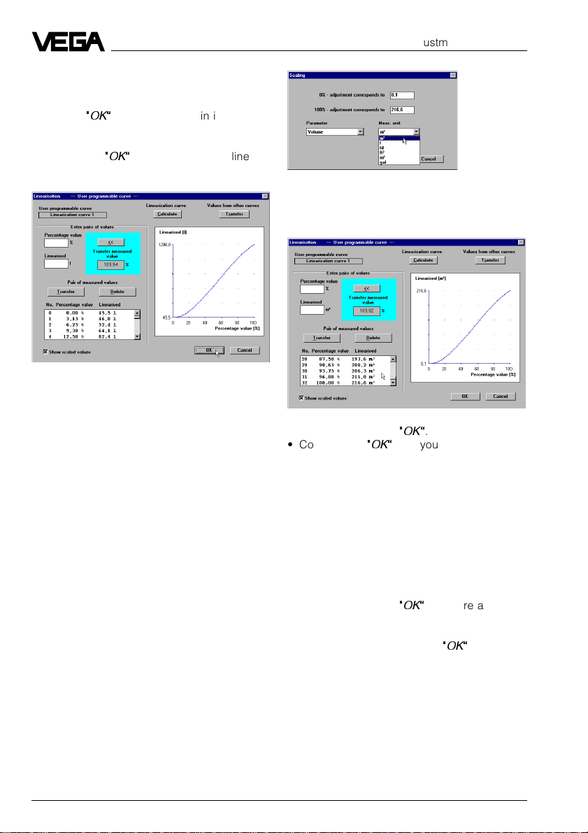
There is a linear interpolation between the linearisation points.

• Click to "OK and you are again in the menu window "

• Again click in the menu window "

culation

sation menu.

Here the calculated linearisation curve is again outputted. The volume information under "

Linearised

longer to the calculated volume of the tank calculation program. Why?

In the menu " tioning/Scaling) you entered that at 0 % filling there are 45 liters in the tank and at 100 % filling 1200 liters. The geometry of the calculated cylindrical tank is reduced to a size that has a volume of only 1200 liters. The linearisation curve of the calculated vessel is therefore modified to fit the volume data you entered in the menu "

If the true content of the calculated vessel should be outputted, the volume that was determined in the tank calculation program must be entered in the menu "Scaling“.

Tank calculation

“.

Tank cal-

“ to "OK and you are in the lineari-

“ now corresponds no

Scaling

“ (Instrument data/Condi-

Scaling

“.

Setup - Adjustment with the PC

The sensor then outputs the actual filling volume by means of the adjusted vessel dimensions.

• Quit the menu with "OK.

• Confirm with "OK and your individual lin-

earisation curve is saved in the sensor.

Again in the menu window " can enter with the menu item "

time

“ a measured value integration. This is recommended for agitated product surfaces, to prevent the measured value indication and output from changing constantly. As a standard feature, an integration time of 0 seconds is preset.

• Quit the menu with "OK., you are again in

the menu window "

eter adjustment

• Quit the menu window with "OK.

“.

Conditioning

“, you

Integration

Instrument data param-

80 VEGASCAN 850

Setup - Adjustment with the PC

Parameter adjustment sensor display

In the menu item "Outputs“ you choose the scale and the unit in which your level should be displayed.

• Choose in the main menu window "

ment data/Parameter adjustment

the menu item "

Outputs

“.

Instru-

“ and then

Meas. loop data

• Click in the window "

rameter adjustment

• Then click to " and "

VEGASCAN

tion on your measurement loop in the information windows.

Instrument data pa-

“ to "

Meas. loop data

Application

“, "

“, to get detailed informa-

Input no.A

“.

“

• In the menu window "

Display of measured value

• Choose the sensor and carry out the adjustments.

• If you want to leave the adjustments unchanged, click to "

• Click in the menu window " "

Quit

“ and you are in the menu window

Instrument data parameter adjustment

• Click in the menu window "

parameter adjustment

VEGASCAN 850 81

Outputs

Quit

“.

“ again to "

“ you click to

“.

Outputs

“ to

“.

Instrument data

Quit

“.

• Close the information window.

• Quit the menu "

• Click in the menu window "Instrument data

parameter adjustment“ to "

You are again in the main menu window.

Meas. loop data

Quit

“.

Setup - Adjustment with the PC

Show measured value

• Click in the main menu window to the menu "

Display/Display of measured value

choose the measurement loop or the sensor to be displayed.

• Choose in the line " output "

Distance

distance will be displayed. When choosing "

Scaled

“, e.g. the measured value will be displayed in liters and volume percent as well as the actual signal current in the 0/4 … 20 mA signal cable.

Indication value

“ and the sensor product

“ and

“ the

Simulation

• Click to the menu " and choose the measurement loop.

The menu window " similar to the previous menu window, opens. In this menu window however, you can set the filling of the vessel or the signal current and the indication to any value (simulate measured value).

First of all, the actual measured value and the signal current are displayed.

• Click to "Start in the turquoise window segment.

Diagnostics/Simulation

Simulation of outputs

“,



82 VEGASCAN 850

Setup - Adjustment with the PC

The grey scrollbar becomes active. With this scrollbar your can modify the measured value in the range of -10 % … 110 % and thereby simulate the filling or emptying of the vessel. In the field of the turquoise window cutout you can enter any % value for the filling percentage.

Choose available linearisation curve

On the previous pages, the entering or the calculation of a linearisation curve was shown as an example. In this menu item, you can choose from the available predefined or userentered linearisation curves.

Note:

The simulated measured value is outputted during adjustment with the PC until you terminate the simulation mode.

A selected curve can be modified later (edit) or calculated with the calculation program.

VEGASCAN 850 83

Print configuration and adjustments

Setup - Adjustment with the PC

• Click to "

Before printing the complete configuration of VEGASCAN and all sensors, you can have a look at the individual pages and …

Services/Print

“.

With the menu " justments displayed in detail.

View

“ you can have the ad-

… then print everything or just certain pages.

84 VEGASCAN 850

Setup - Adjustment with the PC

Backup

With the menu items "

conditioning instruments Backup/Sensors

and parameter settings of VEGASCAN and of each sensor.

The settings can later be quickly transferred to new sensors, e.g. in case of a sensor exchange, or certain product settings can be quickly carried out. This is done in the menu "

Services/Restore configuration

For further information take the manual "VEGA Visual Operating“ (VVO).

Services/Backup/Signal

“ and "

“ you save the configuration

Services/

“.

VEGASCAN 850 85

Setup - Sensor adjustment with the adjustment module MINICOM

6.3 Sensor adjustment with the adjustment module MINICOM

Tank 1 m (d)

12.345

Beside the PC, the ultrasonic sensors VEGASON 51V … 56V can also be adjusted with the small, detachable adjustment module MINICOM in the sensor.

Only the sensor-relevant adjustments such as e.g. scaling of the sensor display, operating range, meas. conditions, sensor display scaling or false echo storage are possible with the adjustment module MINICOM. Not possible are all adjustment steps relating to the configuration, the conditioning and the signal processing (configuration of the inputs and outputs, linearisation curves, simulation …). This is only possible with the PC directly on VEGASCAN 850.

You carry out all adjustment steps with the 6 keys of the adjustment module. A small display shows you, apart from the measured value, a short message on the menu item or on the value of a menu adjustment.

The information volume of the small display, however, cannot be compared with that of the adjustment program VVO, but you will soon get used to it and will be able to carry out your adjustments quickly and directly with the small MINICOM (see menu plan on the following pages).

ESC

1. Measurement in gases

2. Operating range

3. Meas. conditions

4. False echo storage (only necessary, if failures occur during operation).

5. Indication of the useful and noise level

6. Processing/Scaling of the sensor display

In the following you will find the sensor-specific setup items 1 … 6.

1. Measurement in gases

Adjustment is only necessary when the measurement is made in gases (Co2, He, etc.) deviating from air. In case of measurement in gases, sound the distance of the sensor to the product surface and enter it in the menu item "Measurement in gases“. The sensor can then take the modified sonic velocity in gases (as opposed to air) and output correct levels.

2. Operating range

Without special adjustment, the operating range corresponds to the measuring range. The measuring range has already been adjusted with the min./max. adjustment. Generally it is useful to choose a slightly bigger (approx. 5 %) operating range than the measuring range.

Example: Min./max. adjustment: 0.500 … 3.500 m; adjust operating range to approx.

0.400 … 3.600 m.

86 VEGASCAN 850

Setup - Sensor adjustment with the adjustment module MINICOM

3. Meas. conditions

Here you inform each sensor under which application conditions the measurement is carried out, e.g. measurement in gas compositions deviating from air, which will influence the running time of the ultrasonic signals or if a liquid (hard echo) or a solid (weak echo) should be measured.

4. False echo storage

A false echo storage is always useful when unavoidable false echo sources (e.g. struts) must be minimised. By creating a false echo storage, you authorise the sensor electronics to note the false echoes and save them in an internal database. The sensor electronics treats these (false) echoes differently from the useful echoes and filters them out.

5. Useful and noise level

In the menu

you get important information on the signal quality of the product echo. The higher the "S-N“ value, the more reliable the measurement (menu plan MINICOM).

Ampl.:

XX dB

S-N:

Example:

Ampl. = 68 dB S-N = 53 dB

68 dB – 53 dB = 15 dB noise level

53 dB signal level difference indicates very high measurement reliability.

6. Processing/Scaling of the sensor display

(see menu plan)

Ampl.: means amplitude of the level echo in

dB (useful level)

S-N: means Signal-Noise, i.e. the useful

level minus the level of the background noise

The bigger the "S-N“ value (difference between the amplitude useful level and the noise level), the better the measurement: > 50 dB Measurement excellent 40 … 50 dB Measurement very good 20 … 40 dB Measurement good 10 … 20 dB Measurement satisfactory 5 … 10 dB Measurement sufficient < 5 dB Measurement poor

VEGASCAN 850 87

Setup - Sensor adjustment with the adjustment module MINICOM

Menu schematic of the adjustment module MINICOM

Sensor

m(d)

4.700

SON52 V

1.00

When switching on, the sensor type and the software version are displayed for a few seconds.

Parameter

Sensor optimise

Meas. enviro nment

Operating rage

Begin

m (d)

0.50

End

m (d)

6.00

Meas. condit ions

Condit ion

Liquid

Fast change

Measur ing in gas

Meas. dist.

m (d)

4.700

Correc tion Now !

OK ?

Agitat ed sur face

Foaming prod.

Measur ing in gas

False echo memory

Create new

Meas. dist.

m (d)

X.XX

Echo learn Now!

OK ?

learning

Multiple echoes

Update

Meas. dist.

m (d)

X.XX

Update Now!

OK ?

learning

Configuration

Sensor Tag

Sensor

‘Delete

Delete Now!

OK ?

deleting

Meas. unit

m (d)

High

Condit ion

Solid

Fast change

dust level

Large angle repose

Measur ing in gas

Multiple echoes

Displ. adjust ment

Adjust ment in

m(d)

0.0%

m (d)

XX.XXX

Signal condit ioning

Scaling

0 % corres ponds

XXXX

100 % corres ponds

XXXX

Decimalpoint

8888

Prop. to

Volume

Unit

88 VEGASCAN 850

Outputs

Sensor display

Prop. to

Distance

Setup - Sensor adjustment with the adjustment module MINICOM

With these keys you move in the menu field to the left, right, top and bottom

ESC

Basic Reset

Reset Now!

OK ?

reseting

Distance

m (d)

4.700

Ampl.:

XXdB

S-N:

max. range

m (d)

7.000

Add´l functions

Basic

Info

reset

Reset

Sensor Tag

Sensor

Now !

Reseting

Sensor typ

SON 52 V

OK ?

Serial nubmer

1094 8218

Language

English

Softw. Vers.

3.00

Softw. Date

11.09. 1997

Ampl.:

Meas. dist.

X,XX

Fast change

Foaming prod.

Menu items in bolt print provide sensor and measured value information and cannot be modified in this position.

Light grey menu fields are only displayed if required (dependent on the adjustments in other menus).

White menu items can be modified with the "+“ or "–“ key and saved with the "OK“ key.

Distance

m (d)

3.700

S-N:

71dB

Temperature

Actual temp.

Max.

Min.

temp.

°C

VEGASCAN 850 89

7 Diagnostics

Diagnostics

7.1 Simulation

For simulation of a certain filling, you can call up the function "Simulation“ on the adjustment module MINICOM, in the software program VVO or on the signal conditioning instrument.

You simulate a vessel filling and thereby a certain sensor current. Please note that connected instruments, such as e.g. a PLC react according to their adjustments and will probably activate alarms or system functions.

Simulation with VVO

If you start the simulation mode with the adjustment program VVO on the PC, the simulated level is outputted until you quit the simulation mode.

Simulation with MINICOM

If you start the simulation mode on the adjustment module MINICOM, the sensor returns to standard operating mode after one hour.

7.2 Error codes

Error codes Removal

E013 No valid measured value Message is displayed during the warm-up phase

- Sensor in the warm-up phase

- Loss of the useful echo If the message remains, a false echo storage (with the adjustment software on the PC - see “Echo curve” under “Sensor optimisation”) must be carried out together with a modification of mounting location and orientation to achieve the lowest possible false echo background.

E017 Adjustment span too small Carry out a readjustment.

E036 Sensor software does not run Sensor requires new software (service).

E040 Hardware failure/Electronics defec- Check all connection cables.

tive Transducer defective.

90 VEGASCAN 850

Make sure that the difference between min. and max. adjustment is at least 10 mm.

Message appears during a software update.

Contact our service department.

Notes

VEGASCAN 850 91

VEGA Grieshaber KG Am Hohenstein 113 D-77761 Schiltach Phone (0 78 36) 50 - 0 Fax (0 78 36) 50 - 201 e-mail info@vega-g.de internet www.vega-g.de

ISO 9001

The statements on types, application, use and operating conditions of the sensors and processing systems correspond to the latest information at the time of printing.

Technical data subject to alterations

2.24 631 / March 2000

VEGA SCAN850 User Manual

Specifications and Main Features

Frequently Asked Questions

User Manual

Safety information

Note Ex area

1 Product description

1.1 Function

1.2 Application features

1.3 Adjustment

2 Types and versions

2.1 T ype overview, VEGASCAN 850

2.2 T ype overview, sensors

2.3 T ype code, VEGASCAN 850

2.4 T ype code, sensors

2.5 Approvals

2.6 Configuration of measuring systems

3 Technical data

3.1 Data

3.2 Dimensions

4 Mounting and installation

4.1 Mounting VEGASON 54 … 56

4.3 Measurement of liquids

5 Electrical connection

5.1 Connection, connection cable and shielding

5.6 Connection of the PC to VEGASCAN 850

6 Setup

6.1 Adjustment methods

6.2 Adjustment with the PC

7 Diagnostics

7.1 Simulation

7.2 Error codes