VEGA PULS56 User Manual

Download

Operating Instructions

VEGAPULS 56 Profibus PA

Level and Pressure

Contents

Safety information ........................................................................ 3

Note Ex area ................................................................................ 3

1 Product description

1.1 Function................................................................................. 4

1.2 Application features ............................................................. 6

1.3 Profibus output signal .......................................................... 7

1.4 Adjustment ............................................................................ 8

1.5 Antennas............................................................................. 13

2 Types and versions

2.1 Type survey ........................................................................ 14

2.2 Type code........................................................................... 15

2.3 Bus configuration ............................................................... 16

3 Mounting and installation

3.1 General installation instructions ........................................ 22

3.2 Measurement of liquids ..................................................... 24

3.3 Measurement in standpipe (surge or bypass tube) ...... 25

3.4 False echoes ...................................................................... 32

3.5 Installation mistakes ........................................................... 34

Contents

2 VEGAPULS 56 Profibus PA

Contents

4 Electrical connection

4.1 Connection – Connection cable – Screening ................... 36

4.2 Sensor address ................................................................. 39

4.3 Connection of the sensor .................................................. 40

4.4 Connection of the external indicating

instrument VEGADIS 50 .................................................... 42

5 Setup

5.1 Adjustment media .............................................................. 43

5.2 Adjustment with VVO ......................................................... 44

5.3 Sensor adjustment with the adjustment

module MINICOM ............................................................... 66

6 PA function diagram ............................................................... 72

7 Diagnosis

7.1 Simulation ............................................................................ 76

7.2 Error codes ........................................................................ 76

8 Tec hnical data

8.1 Data ..................................................................................... 77

8.2 Approvals ........................................................................... 84

8.3 Data format of the output signal ........................................ 85

8.4 Dimensions ......................................................................... 86

Safety information

Please read this manual carefully, and also take note of country-specific installation standards (e.g. the VDE regulations in Germany) as well as all prevailing safety regulations and accident prevention rules. For safety and warranty reasons, any internal work on the instruments, apart from that involved in normal installation and electrical connection, must be carried out only by qualified VEGA personnel.

VEGAPULS 56 Profibus PA 3

Note Ex area

Please note the attached safety instructions containing important information on installation and operation in Ex areas. These safety instructions are part of the operating instructions and come with the Ex approved instruments.

1 Product description

Level measurement of high temperature processes or products with high temperatures was previously very difficult or even impossible. If such measurement also had to be done under high pressure, there was practically no measuring system available at all, let alone a non-contact measurement system with good measuring accuracy.

Up to now, levels in distillation and stripper columns (e.g. of sump, plate or head products) could usually only be measured by pressure transmitters or differential pressure measurements. The installation required for such pressure measuring systems (pressure cables, pressure transmitters…) is considerable and expensive, often amounting to several times the value of the sensor itself. Because of the lack of suitable alternatives, instrumentation departments have not only had to accept this fact, but also the high maintenance costs (cleaning of measuring pipes, errors by condensation, buildup on the diaphragm…) and the often inadequate accuracy (temperature errors, density fluctuations, installation faults…).

In the petrochemical industry, the requirements for a non-contact level sensor are therefore the following:

• independent of pressure and temperature

• process temperature up to 400°C

• process pressure up to 64 bar

• high resistance wetted parts for universal use

• accuracy 0.1 %

• rugged metal housing

• Ex approved (available in EEx d and EEx ia)

• loop-powered as well as usable in digital networks

This initial set of requirements defined the development goals for the VEGAPULS 56 series, a high-temperature radar level measuring system. The series represents a completely new development of high-temperature radar sensors for temperatures up to 400°C and pressures up to 64 bar.

Product description

These sensors would not have been possible without the recent new results of materials research and production technology. A specially developed ceramic (with highfrequency properties similar to those of the plastics normally used) is used as coupling material. As opposed to plastic, this ceramic has a very high chemical and thermal resistance.

The sensor materials in contact with the process are all highly resistant. This refers not so much to the flange material of high-alloy stainless steel (1.4571 or superior), as to the specially developed ceramic (Al components connecting it. The ceramic rod receives the radar signals from the highfrequency module and acts with its coneshaped end as emitter and receiver. The seal between stainless steel flange and ceramic rod is made with a Tantalum seal ring.

) and the

2O3

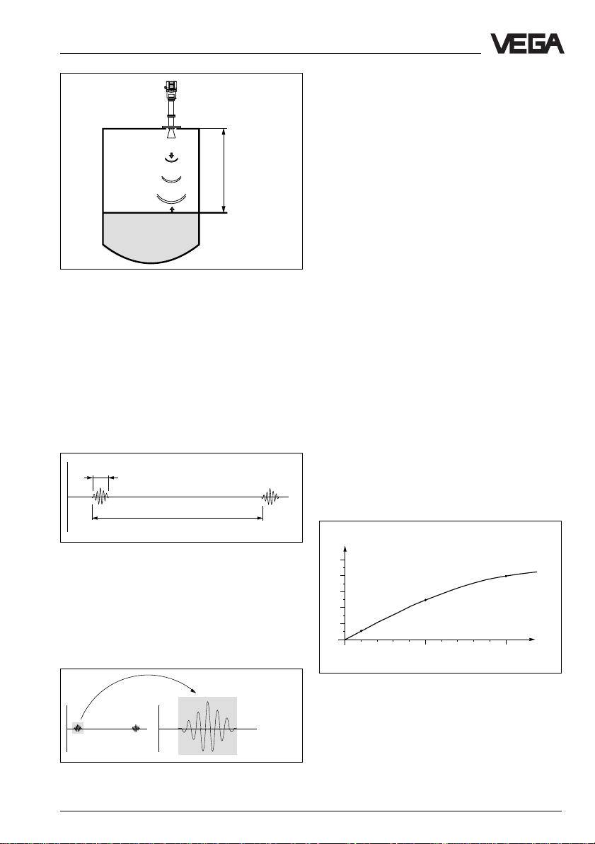
1.1 Function

Radio detecting and ranging: Radar.

VEGAPULS radar sensors are used for noncontact and continuous distance measurement. The measured distance corresponds to a filling height and is outputted as level.

Measuring principle:

emission – reflection – reception

Extremely small 5.8 GHz radar signals are emitted from the antenna of the radar sensor as short pulses. The radar impulses reflected by the sensor environment and the product are received by the antenna as radar echoes. The running period of the radar impulses from emission to reception is proportional to the distance and hence to the level.

4 VEGAPULS 56 Profibus PA

Product description

Meas. distance

emission - reflection - reception

The radar impulses are emitted by the antenna system as impulse packets with a pulse duration of 1 ns and pulse intervals of 278 ns; this corresponds to a pulse package frequency of 3.6 MHz. In the impulse intervals, the antenna system operates as receiver. Signal running periods of less than one billionth of a second must be processed and the echo image evaluated in a fraction of a second.

Through this, it is possible for VEGAPULS series 56 radar sensors to process the slowmotion pictures of the sensor environment precisely and in detail in cycles of 0.5 to 1 second without using time-consuming frequency analysis (e.g. FMCW, required by other radar techniques).

Virtually all products can be measured

Radar signals display physical properties similar to those of visible light. According to the quantum theory, they propagate through empty space. Hence, they are not dependent on a conductive medium (air), and spread out like light at the speed of light. Radar signals react to two basic electrical properties:

- the electrical conductivity of a substance

- the dielectric constant of a substance.

All products which are electrically conductive reflect radar signals very well. Even slightly conductive products ensure a sufficient reflection for a reliable measurement.

1 ns

278 ns

Pulse sequence

VEGAPULS radar sensors can achieve this through a special time transformation procedure which spreads out the more than 3.6 million echo images per second in a slowmotion picture, then freezes and processes them.

All products with a dielectric constant ε more than 2.0 reflect radar impulses sufficiently (note: air has a dielectric constant ε

1).

50 40 30 20 10

5 %

4 6 8 12 14 16 18

25 %

40 %

Reflected radar power dependent on the dielectric constant of the measured product

Time transformation

VEGAPULS 56 Profibus PA 5

Product description

The signal reflection grows stronger with increasing product conductivity or dielectric constant. Hence virtually all products can be measured.

With standard flanges of DN 50 to DN 250, ANSI 2“ to ANSI 10“ the sensor antenna systems can be adapted to various products and measuring environments. The highquality materials of the sensors can also withstand extreme chemical and physical conditions. The sensors deliver stable, reproducible analogue or digital level signals with reliability and precision, and have a long useful life.

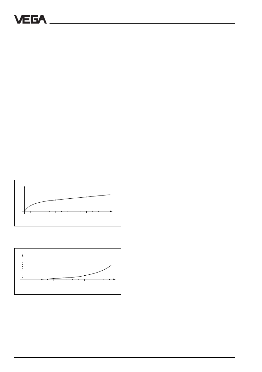
Continuous and reliable

Unaffected by temperature, pressure and individual gas atmospheres, VEGAPULS radar sensors are ideal for non-contact, fast and accurate level measurement of various products.

0,03 0,02 0,01

100 500 1000 1300 ˚C

0,018 %

Temperature influence: Temperature error absolutely zero (e.g. at 500°C 0.018 %)

0,8 %

20 30 40 60

Pressure influence: Error with pressure increase very low (e.g. at 50 bar 1.44 %)

0,023 %

3 %

70 80 90 110 120 130 140

100

bar

1.2 Application features

Applications

• level measurement of liquids, limited use in solids

• measurement also in vacuum

• all slightly conductive materials and all substances with a dielectric constant

> 2.0 can be measured

• measuring ranges 0 … 20 m

Two-wire technology

• power supply and output signal on one two-wire cable

• digital output signal

Rugged and abrasionproof

• non-contact

• high resistance materials

Exact and reliable

• resolution 1 mm

• unaffected by noise, vapours, dusts, gas compositions and inert gas stratification

• unaffected by varying density and temperature of the medium

• measurement of pressures up to 64 bar and product temperatures up to 350°C

Communicative

• individual wiring, with 15 sensors on one two-wire cable (digital output signal)

• integrated measured value display

• optional display module up to 25 m separate from the sensor

• connection to all bus systems: Interbus S, Modbus, Siemens 3964R, Profibus DP, Profibus FMS, ASCII

• adjustment from PLC level

Ex approvals

• CENELEC, FM, ABS, LRS, GL, LR, ATEX, PTB, FCC

VEGAPULS series 56 sensors enable level measurement with radar in systems where it was previously not used due to high costs.

6 VEGAPULS 56 Profibus PA

Product description

1.3 Profibus output signal

PROPRO

PROcess

PROPRO sult of a joint project of thirteen companies and five universities. The companies Bosch, Klöckner-Möller and Siemens played a decisive role. The specifications of the bus are described in the protocol layers 1, 2 and 7 of the ISO/OSI reference model and are available from the PNO (Profibus User Organisation). Layers 3 … 5 have not yet been developed as a standard, leaving Profibus with far-reaching perspectives for the future.

Today approx. 600 companies make use of Profibus technology and belong to the PNO, Profibus Specification. Profibus Periphery and Profibus mation.

As a process automation bus, Profibus PA enables power supply over the bus. Up to 32 sensors with power supply and measuring signal can be operated on a shielded twowire cable that carries both power supply and measuring signal. In Ex areas, up to ten sensors can be connected from the PA level to one two-wire cable (EEx ia).

Bus structure

A Profibus system with DP and PA segments consists of up to 126 Master and Slave participants. Data are always exchanged from point to point, with the data traffic being exclusively controlled and checked by master devices. Communication is carried out according to the Token-Passing procedure. This means that the master holding the Token can contact the slaves, give instructions, enquire data and cause the slaves to receive and transmit data. After the work is done or after a predetermined time interval, the Token is passed on by the master to the next master.

FIFI

BUSBUS

FIeld

BUS (PROFIBUS) is the re-

FIFI

BUSBUS

FMSFMS

FMS stands for Fieldbus Messaging

FMSFMS

DPDP

DP for Decentralised

DPDP

A for Process Auto-

Master-Class 1

is the actual automation system, i.e. the process control computer or the PLC that enquires and processes all measured values.

Master-Class 2

One or several Master-Class 2 can operate in a Profibus network. As a rule, Master-Class 2 devices are engineering, adjustment or visualisation stations. The VEGA adjustment software VVO (VEGA Visual Operating) operates as Master-Class 2 participant on the DP bus and can work on an engineering PC, on an adjustment PC or on the process control computer and can access any VEGA sensor on the PA level.

Instrument master file

A so-called GSD (instrument master file) is provided with the VEGAPULS Profibus sensor. This file is necessary to integrate the sensor in the bus system. The GSD contains, beside the sensor name and manufacturer, the sensor-specific communication parameters which are necessary for a stable integration of the sensor in the bus.

Load the GSD belonging to the sensor into your bus configuration program. If the GSD is not available, it can be downloaded from the VEGA homepage: http://www.vega.com.

Do not mistake the GSD for the EDD (Electronic Device Description), which is necessary for the PDM environment and can also be found on the VEGA homepage.

VEGAPULS 56 Profibus PA 7

Product description

1.4 Adjustment

Each measuring situation is unique. For that reason, every radar sensor needs some basic information on the application and the environment, e.g. which level means "empty" and which level "full". Beside this "empty and full adjustment", many other settings and adjustments are possible with VEGAPULS radar sensors. The output of echo curves or the calculation of vessel linearisation curves by means of vessel dimensions are only two examples.

Profibus adjustment structure

In the Profibus environment, there are different adjustment concepts and adjustment tools which often differ considerably from manufacturer to manufacturer. From the user’s point of view, a manufacturer-independent adjustment program which could be operated directly on the Profibus DP, as well as at any system node (e.g. the engineering station or the process control), would be ideal.

In the past, only the program "SIMATIC PDM“, based on the HART ture, could fulfil this wish (though with the limitations common to HART

HART

, the availability of an instrument-specific database for a comprehensive adjustment with PDM (Process Device Managing) is a requirement. Otherwise, only the basic instrument functions, such as adjustment, are available. In the PDM environment, this instrument-specific database is called EDD (Electronic Device Description), in perfect analogy to the HART

environment which also requires, except for the VEGA HART ments, a DD (Device Description) for each sensor.

adjustment struc-

). As with

instru-

We are aware of the disadvantages of the

HART

environment: for each sensor/participant, an individual DD must be loaded, which in addition, must always be the latest and most up-to-date DD. Special adjustment options such as e.g., the output of an echo curve, are available neither with HART

nor with PDM. User-friendly adjustment is out of the question. With VEGA’s adjustment program VVO, those restrictions belong to the past.

The legitimate wish of many Profibus users for a manufacturer-independent adjustment tool without EDD has been realised in the form of PACTware number of process technology companies developed PACTware

TM 1)

. An association of a

: a Process Automation Configuration Tool that can run different manufacturer software tools under a standardized user interface and adjustment structure. Specialists call this technology Field Device Transcription. Just as different Windows printer drivers enable operation of completely different printers under a single user interface, PACTware

enables operation of all field instruments under a single user interface. Instrument-specific databases (EDD), like those required for SIMATIC PDM, are not necessary.

As a result of this development, three adjustment media are available for VEGA-Profibus sensors:

- adjustment with the PC and the adjustment

program VVO (VEGA Visual Operating) as stand-alone tool, on the segment coupler or directly on the sensor.

- adjustment with the detachable adjustment

module MINICOM in the sensor

- adjustment with the SIMATIC PDM adjust-

ment program (requires EDD instrument databases) from the control room.

- adjustment with the universal adjustment

interface PACTware

on the sensor, from

the control room or on the segment coupler.

8 VEGAPULS 56 Profibus PA

Product description

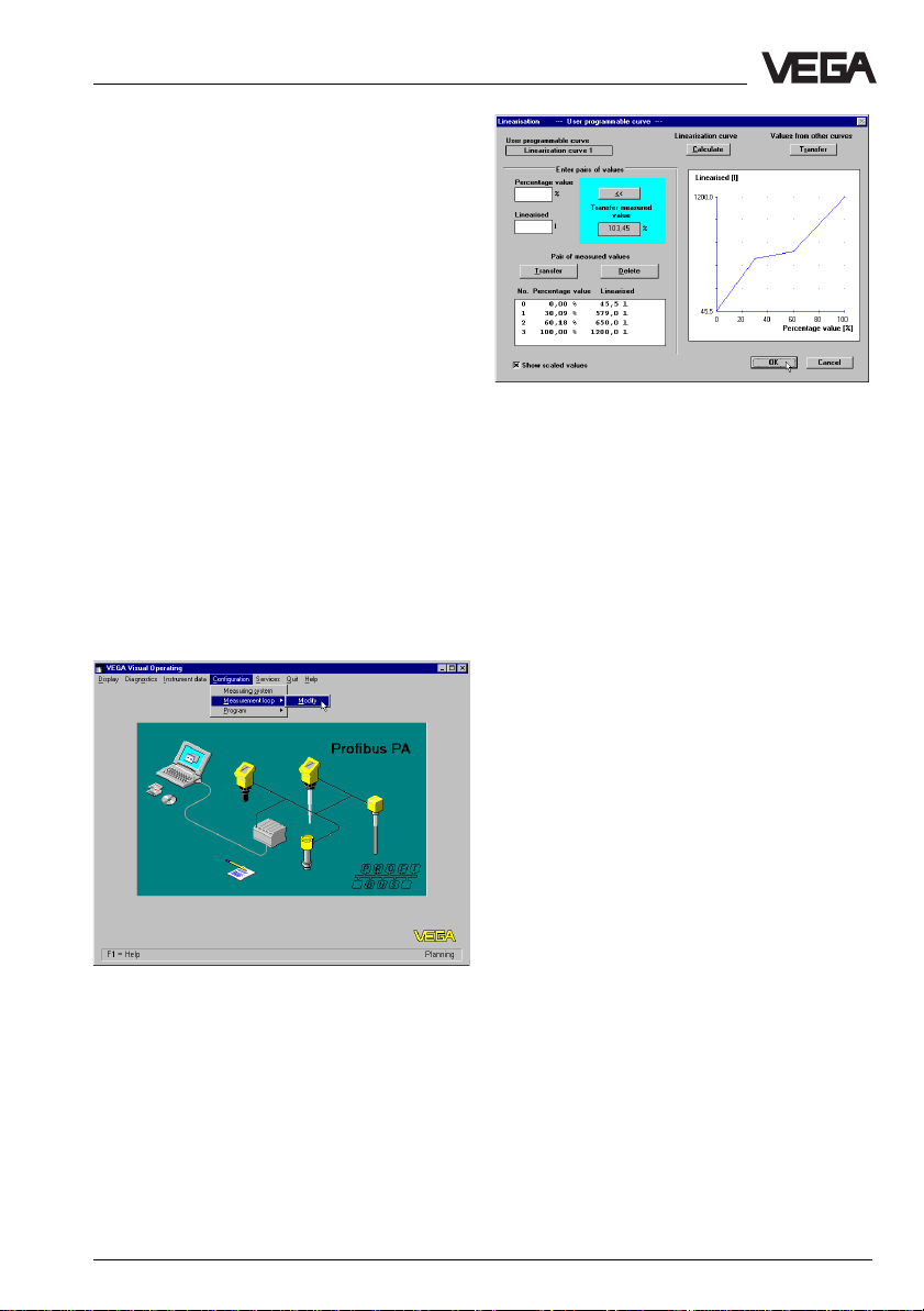
Adjustment with the adjustment program VVO - VEGA Visual Operating

The setup and adjustment of the radar sensors is generally done on the PC with the adjustment program VEGA Visual Operating (VVO) or with PACTware The programs lead quickly through adjustment and parameter setting by means of pictures, graphics and process visualisations.

under Windows®.

Note:

The adjustment program VVO must be available in version 2.70 or higher.

The VEGA adjustment software VVO (VEGA Visual Operating) operates either as a subprogram of the host program PACTware

acc. to the FDT concept (Field Device Tool) or as an independent adjustment program on any PC, engineering station or process control computer.

The adjustment program recognises the sensor type

Visualised input of a vessel linearisation curve in the adjustment program VVO

VEGA’s adjustment program VVO can access the adjustment options of VEGA sensors in their entirety and, if necessary, can update the complete sensor software. To do this, the adjustment program must be installed on a PC which is equipped with a Profibus Master Class 2 interface card or the interface adapter VEGACONNECT 3.

The PC with the Profibus interface card can be connected directly to any point on the DP bus with the standard RS 485 Profibus cable.

In conjunction with the adapter VEGACONNECT, the PC can be connected directly to the sensor. VEGACONNECT communicates via a small jack directly with the respective sensor.

The adjustment and parameter data can be saved at any time on the PC with the adjustment software and can be protected by passwords. If necessary, the adjustments can be transferred quickly to other sensors.

VEGAPULS 56 Profibus PA 9

In practice, the adjustment program VVO is often installed as a tool on an engineering station or operating station. VVO then accesses all VEGA sensors directly over the bus via the Profibus interface card (e.g. from Softing) as Master Class 2, from the DP level to the PA level (via segment coupler) right down to the individual sensor.

Beside the instrument master file (GSD), with which a sensor is logged into the Profibus system, the majority of all Profibus sensors requires for adjustment, beside the specific adjustment software, also a so-called EDD (Electronic Device Description) for each sensor, in order to access and adjust the sensor from the bus levels. This is not the case with VVO. The adjustment software VVO can communicate at any time with all VEGA sensors without the help of a special database. Of course, all other non-Profibus VEGA sensors can be adjusted with the adjustment software as well (4 … 20 mA sensors or VBUS sensors). With VEGA sensors, it is not necessary to go looking for the latest EDD. This is the basic prerequisite for a manufacturer-independent adjustment program, like PACTware

, anticipated by

many users, see following pages.

Product description

10 VEGAPULS 56 Profibus PA

Product description

Adr. 21

SPS

Adr. 22

VVO

PA-

Adr. 23

Bus

Master-Class 1

Adr. 1

DP-Bus

Adr. 24

Profibus DP interface card as Master-Class 2 (e.g. Softing)

Adr. 10

Adr. 57

Segment coupler

Adr. 25 … 56

Adr. 58

Adr. 59

(max. 32 participants)

Adr. 60

Adr. 26

Adr. 25

Adr. 27

Adr. 28

Adr. 29

Adjustment of the VEGAPULS radar sensors from process control via a Profibus interface card in the process control computer or in an additional PC. The adjustment software VEGA Visual Operating (VVO) accesses via the interface (interface card) the sensors bidirectionally.

VEGAPULS 56 Profibus PA 11

Product description

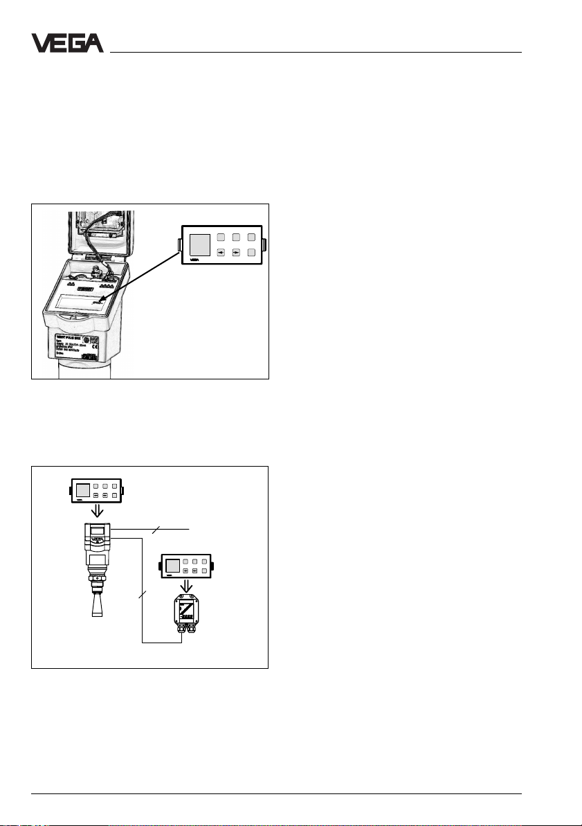
Adjustment with adjustment module MINICOM

With the small (3.2 cm x 6.7 cm) 6-key adjustment module with display, you carry out the adjustment in clear text dialogue. The adjustment module can be plugged into the radar sensor or into the optional, external indicating instrument.

Tank 1

m (d)

12.345

Detachable adjustment module MINICOM

The adjustment module can be removed easily so that unauthorised people cannot modify the sensor setting.

ESC

Tank 1 m (d)

12.345

PA-Bus

ESC

Tank 1 m (d)

12.345

Adjustment with the SIMATIC PDM adjustment program

For adjustment of all essential functions of the VEGA sensor with the adjustment station SIMATIC PDM from Siemens, a so-called EDD is required. Without this EDD, only the basic functions such as min./max. wet adjustment or integration time can be adjusted with the PDM adjustment program. Further important adjustment functions, such as the input of the "

Meas. environment

storage are not available without EDD. After

ESC

integration of the EDD files in the Simatic PDM

adjustment software, all important adjustment

“ or a false echo

functions are accessible. If it is not at hand, the obligatory GSD (instrument master file) as well as the EDD (Electronic Device Description) necessary for PDM can be downloaded from the VEGA-Homepage (http://www.vega.com).

Adjustment with PACTware

The above-mentioned program PACTware is a manufacturer-independent automation/ configuration tool, by which access to instruments of different manufacturers (Krohne, Pepperl + Fuchs, VEGA, VIKA- Bürkert…) is possible. The VEGA adjustment software VVO works as a subprogram/menu. PACTware options for the sensor/instrument being accessed.

PACTware constructed in tree structure. Operating instructions for PACTware the PACTwareTM documentation. They are not described in this operating instructions manual.

activates the required menu

looks different than VVO and is

can be found in

max. 25 m

Adjustment with detachable adjustment module. The adjustment module can be plugged into the radar sensor or into the external indicating instrument VEGADIS 50.

12 VEGAPULS 56 Profibus PA

Product description

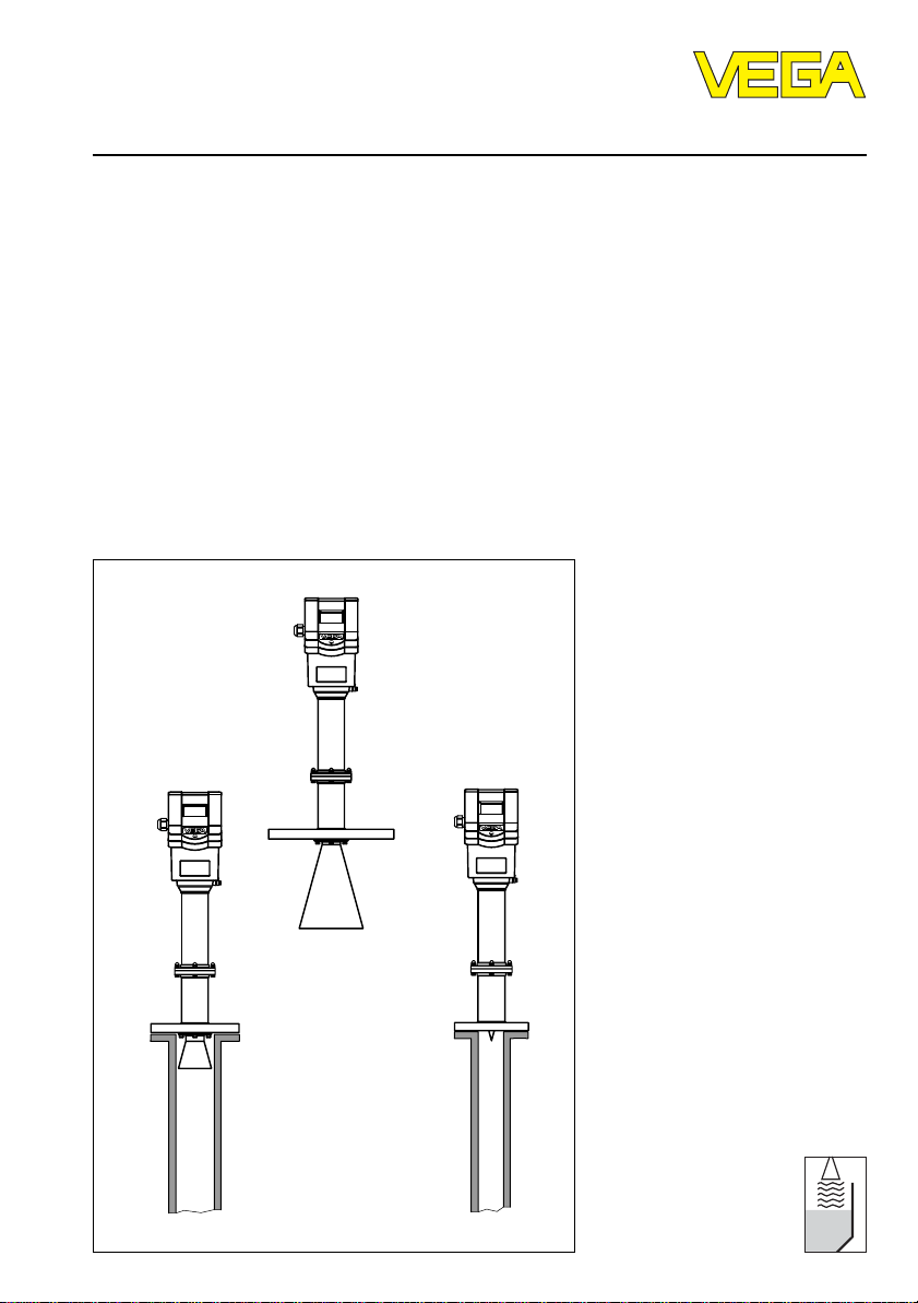
1.5 Antennas

The antenna is the eye of the radar sensor. An uninitiated observer would probably not realise how carefully the antenna geometry must be adapted to the physical properties of electromagnetic fields. The geometrical form determines focal properties and sensitivity - the same way it determines the sensitivity of a unidirectional microphone.

For different applications and process requirements various antenna systems are available.

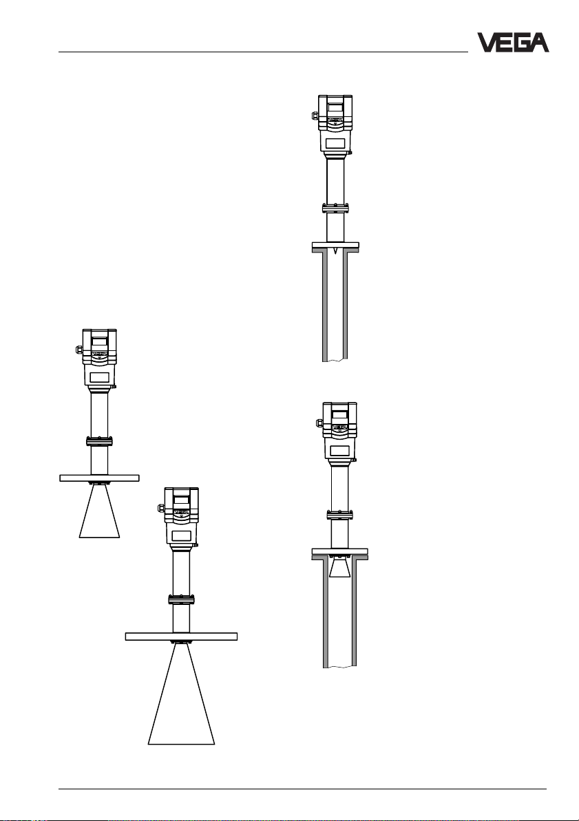
Horn antenna

Horn antennas focus the radar signals very well. Made of 1.4571 (stainless steel) or Hastelloy C22 they are very rugged, and physically as well as chemically resistant. Horn antennas are used for measurement in closed or open vessels.

Pipe antenna

Only in conjunction with a measuring tube, i.e. with a surge or bypass tube (which can also be angled), do horn antennas form a complete antenna system. Pipe antennas are mainly suitable for very agitated products or for products with very small dielectric constant.

The antenna can be with or without horn. The antennas are characterised by a very high antenna gain. High reliability can be achieved even with products having poor reflective properties.

For the radar signals, the measuring tube acts as a conductor.

DN 50

The running time of the radar signal changes in the tube and depends on the tube diameter.

Therefore, the sensor must be informed about the tube inner diameter so that the change in the running time can be taken into account and precise level signals ensured.

DN 150

DN 80

DN 250

VEGAPULS 56 Profibus PA 13

2 Types and versions

VEGAPULS 56 sensors are a newly developed generation of very compact, high temperature radar sensors. They enable for the first time non-contact level measurements under high temperatures and pressures. They offer the advantages of radar level measurement for applications in which the special advantages of radar could not be previously applied due to extreme process conditions.

VEGAPULS 56 radar sensors utilise two-wire technology perfectly. The supply voltage and the output signal are transmitted via one twowire cable. They provide an analogue 4 … 20 mA output signal as output or measuring signal. This operating instructions manual describes the sensors with digital output signal.

Types and versions

2.1 Type surve y

General features

• Level measurement of processes and products under high temperatures and high pressures

• Measuring range 0 … 20 m

• Ex approved in Zone 1 and Zone 10 (IEC) or Zone 0 and Zone 20 (ATEX) classification mark EEx ia IIC T6 or EEx d ia IIC T6

• Integrated measured value display

• External measured value display which can be mounted at a distance of up to 25 m in Ex area

Survey of features

Signal output

- digital transmission of measuring signals to a VEGAMET signal conditioning instrument or the VEGALOG processing system

VEGAPULS 56 DN 150

VEGAPULS 56 DN 50 pipe antenna

VEGAPULS 56 DN 80 pipe antenna

Power supply – two-wire technology (voltage supply and

digital signal via one two-wire cable)

Process fitting – DN 50; ANSI 2“ – DN 80; ANSI 3“ – DN 100; ANSI 4“ – DN 150; ANSI 6“ – DN 200; ANSI 8“ – DN 250; ANSI 10“

Adjustment –PC – adjustment module in the sensor – adjustment module in external indicating

instrument

Antennas – horn antenna with stainless steel horn and

ceramic tip

– standpipe antenna only with ceramic tip or

with small horn and ceramic tip

14 VEGAPULS 56 Profibus PA

Types and versions

2.2 Type code

56… High temperature radar sensor …K 4 … 20 mA output signal (not described in this operating instruction manual) …P Output signal Profibus PA

VEGAPULS 56 V EXXX X X X X X X X

J - Tube extension for horn antenna X - without

A - Aluminium housing D - Aluminium housing with Exd connection housing

T - Seal of the antenna system of Tantalum

KVX - Process fitting DN 50 PN 16 (for standpipe) LV6 - Process fitting DN 80 PN 16 (for standpipe) EV1 - Process fitting DN 100 PN 16 (for standpipe) FV2 - Process fitting DN 150 PN 16 SVX - Pr ocess fitting ANSI 2“ 150 psi (for standpipe) WV6 - Process fitting ANSI 3“ 150 psi (for standpipe) PV1 - Process fitting ANSI 4“ 150 psi (for standpipe) VV2 - Process fitting ANSI 6“ 150 psi 0V2 - Process fitting ANSI 6“ 300 psi 1V2 - Process fitting ANSI 6“ 600 psi (1.4571) 1M2 - Process fitting ANSI 6“ 600 psi (Hastelloy C22) YYY - Ot her pr ocess connections and materials

X - without display A - with integrated display

X - without adjustment module MINICOM

B - with adjustment module MINICOM (mounted)

B - 20 … 72 V DC; 20 … 250 V AC; 4 … 20 mA; HART D - Two-wire (loop-powered); 4 … 20 mA; HART E - Power supply via signal conditioning instrument G - Profibus PA (power supply from segment coupler) P - 90 … 250 V AC (only in USA) N - 20 … 36 V DC, 24 V AC (only in USA) Z - Power supply via signal conditioning instrument (only in USA)

.X - FTZ approval (Germany) EX.X - Approved Zone 1 and Zone 10 EX0.X - Ex approved Zone 0

K - Analogue 4 … 20 mA output signal

(two-wire technology)

P - Digital output signal (two-wire technology) Profibus

Instrument series for high temperature application

Measuring technology (PULS for radar)

VEGAPULS 56 Profibus PA 15

Types and versions

2.3 Bus configuration

The type of radar sensor you use depends on your process requirements and mounting conditions, as well as on the requirements of your control, regulative, or process control system.

VEGAPULS 56 Profibus radar sensors are sensors for use in Profibus PA environment. Profile 3 has been implemented in the sensors. A measuring system consists of one or several sensors, one or several segment couplers and one DP master computer, such as e.g. a S7 PLC with Profibus interface or a process control system with Profibus DPMaster-Slot. The processing unit, e.g. the PLC, evaluates the level-proportional, digital measuring signals in a number of evaluation routines and puts them to use process-specifically.

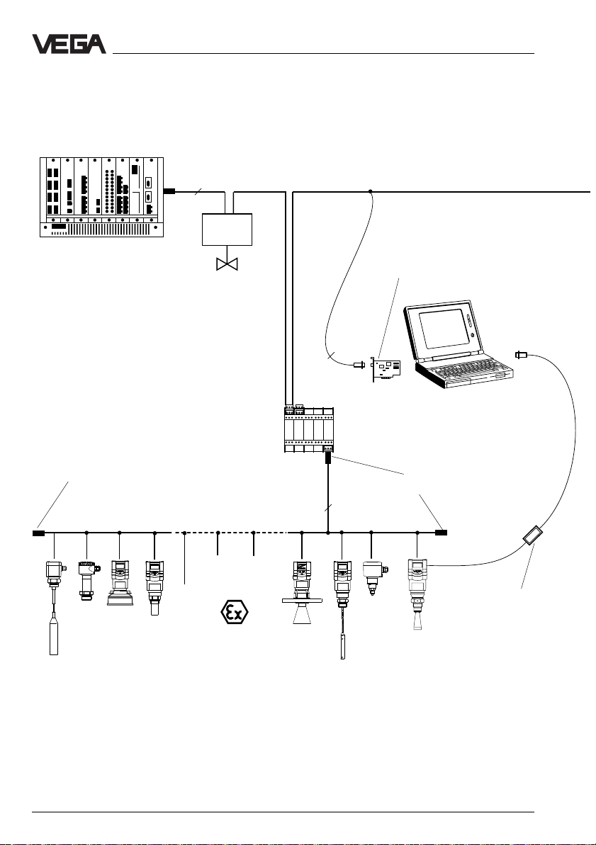
On the following four pages you will see schematic illustrations of the bus configuration.

The automation system as Master-Class 1 takes over bus control completely. It reads out all signals cyclically and, if necessary, gives instructions to the participants (e.g. sensors). Besides this, additional master systems (e.g. visualisation systems or adjustment tools) can be connected to the DP bus. These systems operate as so-called Master-Class 2 participants. Like the MasterClass 1 system, they can read out signals, give instructions and operate in the acyclical mode.

A DP bus does not allow power supply via signal cable, whereas the PA bus does. Both, DP and PA, require at a minimum a screened two-wire cable. The DP bus can additionally have up to 8 cores (screened), of which some can be supply cables (see also "Installation Guides PA + DP“ of the Profibus User Organisation (PNO).

Each participant on the bus must have an unambiguous address. The addressing covers both bus levels. A Profibus DP network can have max. 126 participants, including all participants on the PA level. In practice, each Master-Class 1 computer gets address 1 and the Master-Class 2 computers address 10 … 20. As a rule, the slaves or participants get the addresses 21 … 126. On the Profibus PA network segment, max. 32 sensors are possible on one PA segment coupler.

Ex environment

In Ex environment, intrinsically safe (EEx ia) PA sensors are used with Ex segment couplers. Generally, the number of PA sensors on a segment coupler (Ex or non Ex) depends on the current requirement of the sensors and on the current supplied by the segment coupler. Segment couplers for EEx ia environment provide 90 … 110 mA. The number of sensors results from the sum of:

- the basic current intake of all sensors

- plus 9 mA communication signal

- plus the leakage currents of all sensors

- plus a recommended current reserve (approx. 10 mA)

The min. basic current has been set at 10 mA according to the Profibus specification. VEGA Profibus sensors constantly consume a basic current of 10 mA and operate without leakage current requirement, so that in Ex environment, up to max. ten VEGA sensors can be operated on one segment coupler.

16 VEGAPULS 56 Profibus PA

Types and versions

VEGAPULS 56 Profibus PA 17

Types and versions

Master-Class 1

Bus terminator

3...9

Profibus PA (31,25 kBit/s)

Profibus DP

Profibus interface card

RS 232

22...54

RS 485

Master-Class 2

Segment coupler

Bus terminator

VEGACONNECT 3

PA segment on segment coupler: 1 … 32 sensors on one two-wire cable (Ex: 10 sensors)

18 VEGAPULS 56 Profibus PA

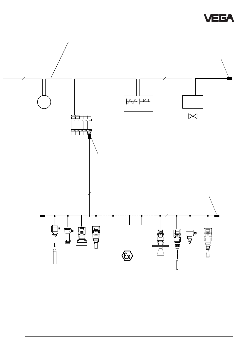
Types and versions

Profibus DP segment level 1 … 126 participants including all DP and PA participants. Through segment couplers and PA segments, the transmission rate, also on the DP level, is determined by the slowest coupler or participant on the Profibus DP and PA network.

Bus terminator

3...9

Segment coupler

3...9

3~M

56...88

Bus terminator

Profibus PA

Bus terminator

PA segment on segment coupler: 1 … 32 sensors on one two-wire cable (Ex: 10 sensors)

VEGAPULS 56 Profibus PA 19

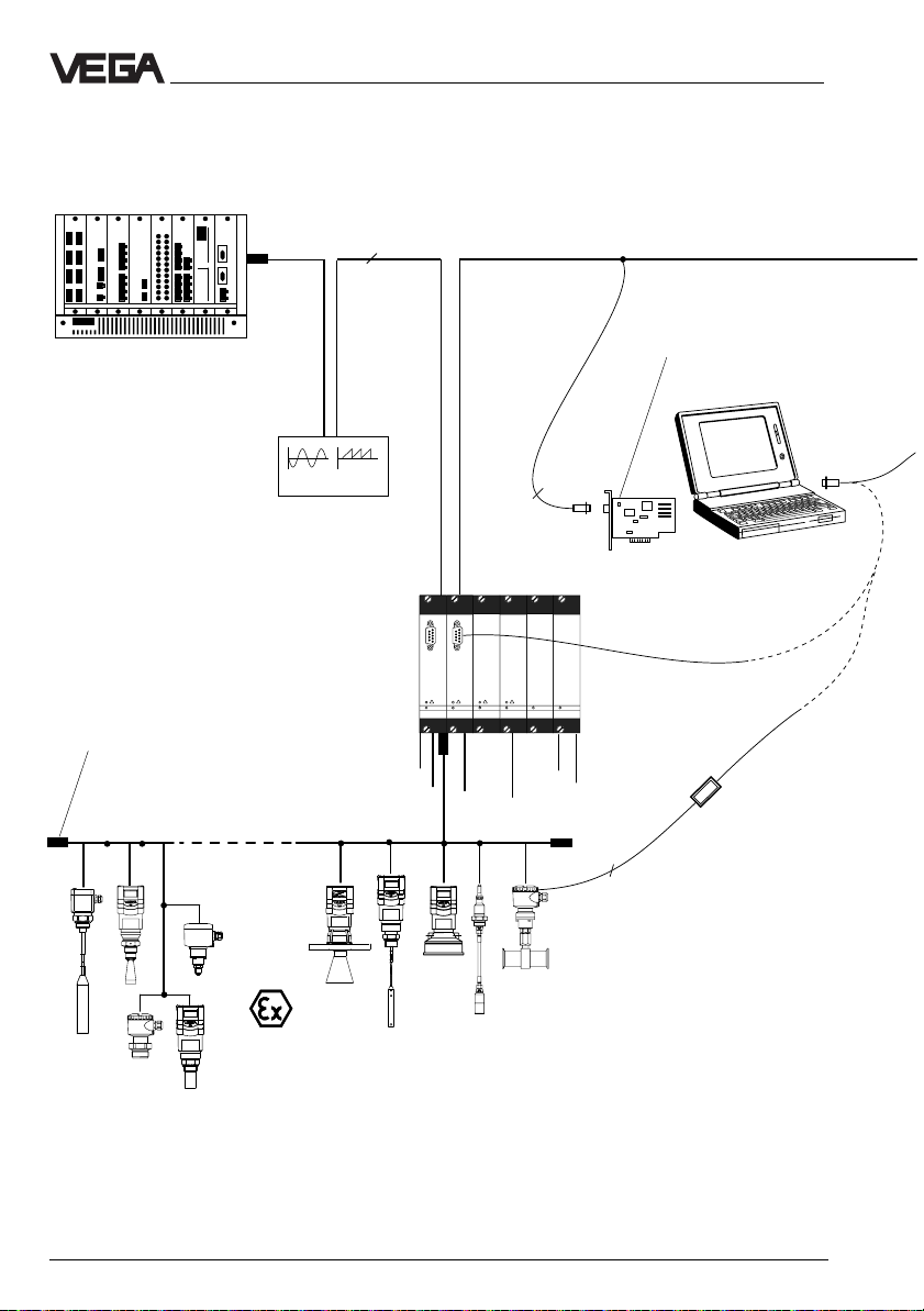
Types and versions

Master-Class 1

Bus terminator

VEGALOG

Profibus PA (31,25 kBit)

3~M

3…9

Profibus DP

Profibus interface card

RS 485

Master-Class 2

VEGACONNECT 3

RS 232

1 … 15 PA sensors per two-wire cable

with independent address zone (Ex: 10 sensors)

20 VEGAPULS 56 Profibus PA

Types and versions

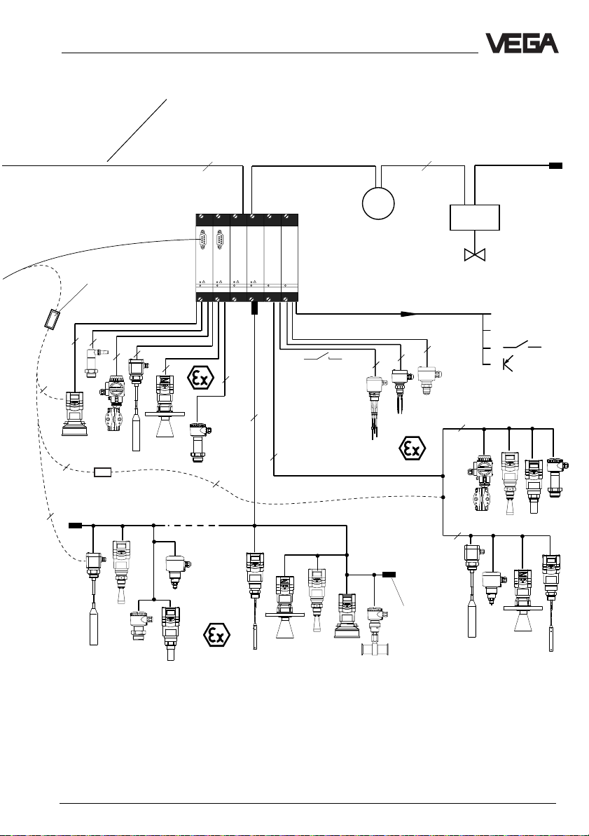
Profibus DP segment level 1 … 126 participants including all DP and PA participants. Up to 12 MBit/s transmission rate on DP level. In the PA segments 31.25 kBit/s transmission rate.

VEGACONNECT 3

4 … 20 mA (HART )

Profibus PA (31,25 kBit)

3…9

VEGALOG

VBUS

Outputs

0/4…20 mA

0…10 V

VBUS

Bus terminator

Profibus PA: 1 … 15 PA sensors per two-wire cable with independent address zone (Ex: 10 sensors)

VBUS: 1 … 15 sensors per twowire cable Exd: also 15 Ex ia: 5 sensors

VEGAPULS 56 Profibus PA 21

;;

3 Mounting and installation

3.1 General installation instructions

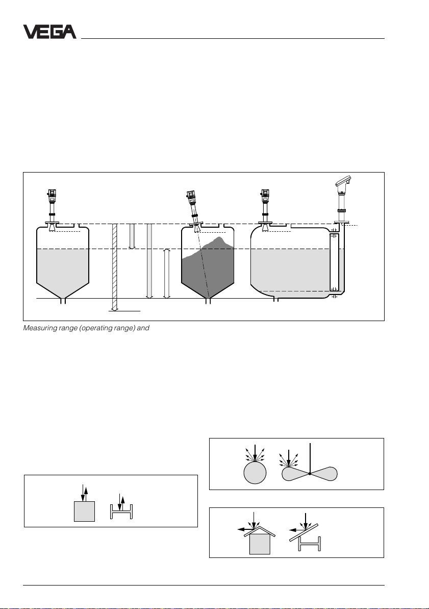
Measuring range

The reference plane for the measuring range of the sensors is the lower edge of the flange. The measuring range is 0 … 20 m. For measurement in surge or bypass tubes (pipe antenna) the max. measuring distance is reduced (see "Technical data - Measuring range“).

Mounting and installation

Keep in mind that in measuring environments where the medium can reach the sensor flange, buildup can form on the antenna which can cause measurement errors. The min. distance of the antenna to the medium should be 5 cm.

Reference plane

min. meas. distance

full

min.

Meas. range

empty

max. meas. distance 20 m

Measuring range (operating range) and max. measuring distance Note: Use of the sensors for applications with solids is limited.

False reflections

Flat obstructions and struts cause large false reflections. They reflect the radar signal with high energy density.

Interfering surfaces with a round profile diffuse the reflected radar signals and cause

If flat obstructions in the range of the radar signals cannot be avoided, we recommend the installation of a deflector plate to scatter the reflected signals. Due to this scattering, the interfering signals will be low in amplitude and so diffuse that they can be filtered out by the sensor.

false reflections with lower energy density. Hence, they are less critical than reflections from a flat surface.

Round profiles diffuse radar signals

min. meas. distance

full

empty

Profile with smooth interfering surfaces cause large false signals

22 VEGAPULS 56 Profibus PA

A deflector causes signal scattering

Mounting and installation

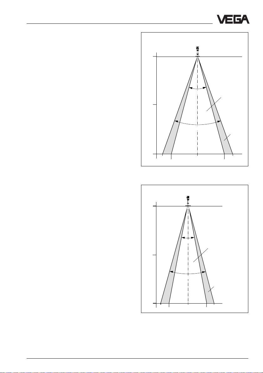
Emission cone and false reflections

The radar signals are focused by the antenna system. The signals leave the antenna in a conical path similar to the beam pattern of a spotlight. This emission cone depends on the antenna used.

Any object in this beam cone causes a reflection of the radar signals. Within the first few meters of the beam cone, tubes, struts or other installations can interfere with the measurement. At a distance of 6 m, the false echo of a strut has an amplitude nine times greater than at a distance of 18 m.

At greater distances, the energy of the radar signal distributes itself over a larger area, thus causing weaker echoes from obstructing surfaces. The interfering signals are therefore less critical than those at close range.

If possible, orient the sensor axis perpendicularly to the product surface and avoid vessel installations (e.g. pipes and struts) within the 100 % area of the emission cone.

If possible, provide a "clear view“ of the product inside the emission cone and avoid vessel installations in the first third of the emission cone.

Meas. distance

0 m

30˚

10 m

40˚

20 m

6,8 m 6,8 m

Emission cone of a DN 100 horn antenna

Meas. distance

0 m

100 %

emitted power

50 %

5,3 m5,3 m

Optimum measuring conditions exist when the emission cone reaches the measured product perpendicularly and when the emission cone is free from obstructions.

10 m

20 m

5,0 m

3,5 m

Emission cone of a DN 150 horn antenna

VEGAPULS 56 Profibus PA 23

20˚

30˚

100 %

emitted power

50 %

emitted power

5,0 m

3,5 m

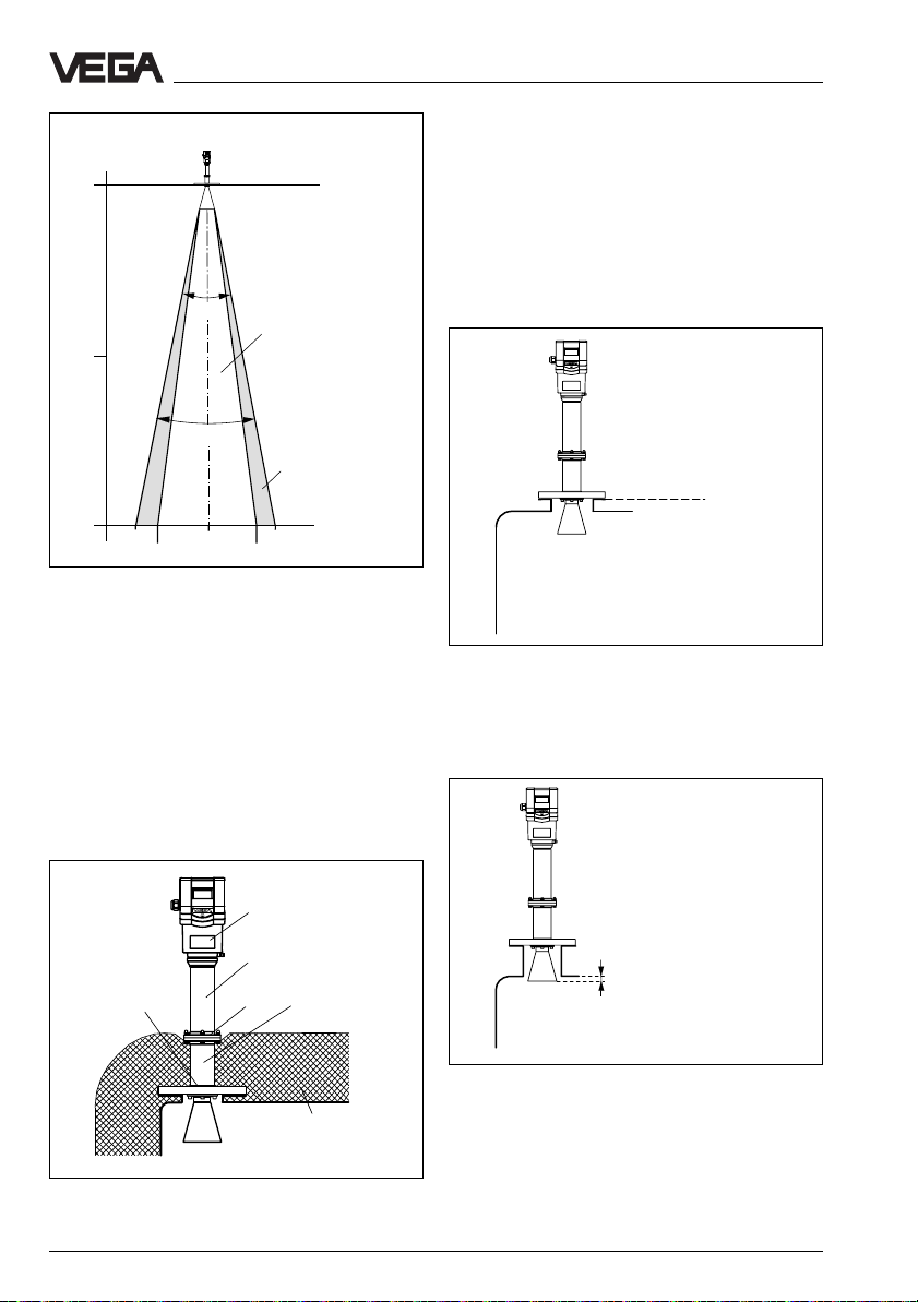
Mounting and installation

Meas. distance

0 m

14˚

100 %

22˚

emitted power

50 %

3,8 m

2,4 m

emitted power

10 m

20 m

3,8 m

2,4 m

Emission cone of a DN 250 horn antenna

Heat insulation

In process temperatures of more than 200°C the rear of the flange must be insulated to protect the sensor electronics from radiated heat.

We recommend integrating the sensor insulation into the vessel insulation and extending it approx. up to the first tube segment.

3.2 Measurement of liquids

Sensor on DIN socket piece

Most commonly, the mounting of radar sensors is done on short DIN socket pieces. The lower side of the instrument flange is the reference plane for the measuring range. The antenna should always protrude out of the flange pipe.

Reference plane

Mounting on DIN socket piece

With a longer DIN socket piece, the horn antenna must protrude at least 10 mm out of the socket.

40°C

60°C

> 10 mm

350°C

100°C

240°C

Mounting on longer DIN socket piece

Vessel insulation

max. 350°C

When mounting on dished vessel tops, the antenna must also protrude at least 10 mm beyond the longer side of the socket).

Heat insulation

24 VEGAPULS 56 Profibus PA

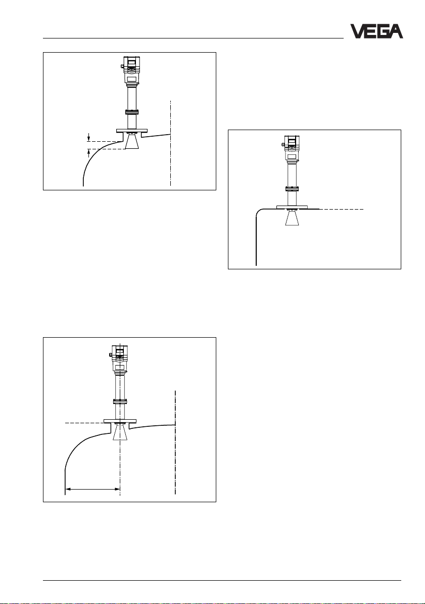
Mounting and installation

> 10 mm

Sensor directly on the vessel top

If the stability of the vessel will allow it (sensor weight), flat mounting directly on the vessel top is a good and economical solution. The top side of the vessel is the reference plane.

Mounting on a dished vessel top

On dished tank ends, please do not mount the instrument in the centre or close to the vessel wall, but approx.

/2 vessel radius from

the centre or from the vessel wall.

Dished tank ends can act as paraboloidal reflectors. If the radar sensor is placed in the focal point of the parabolic tank, the radar sensor receives amplified false echoes. The radar sensor should be mounted outside the focal point. Parabolically amplified echoes are thereby avoided.

Reference plane

/2 vessel radius

Mounting on dished tank ends

Reference plane

Mounting directly on the flat vessel top

3.3 Measurement in standpipe (surge or bypass tube)

General instructions

Pipe antennas are preferred in vessels which contain many installations, e.g. heating tubes, heat exchangers or fast-running stirrers. Measurement is then possible where the product surface is very turbulent, and vessel installations cannot cause false echoes.

Through focusing of the radar signal within the measuring tube, even products with small dielectric constants (ε reliably measured in surge or bypass tubes. Please note the following instructions.

Surge pipes which are open at the bottom must extend over the full measuring range (i.e. down to 0% level), as a measurement is only possible within the tube.

It is advantageous to install a deflector below the end of the tube. The product can then be reliably detected around the min. level. This is particularly important for products with a dielectric constant of less than 5.

= 1.6 up to 3) can be

VEGAPULS 56 Profibus PA 25

;;;

;

Mounting and installation

Surge pipe welded to the tank

Surge pipe in the socket piece

Marking holes in the intermediate flange

max.

Vent hole

Deflector

min.

Pipe antenna systems in the tank

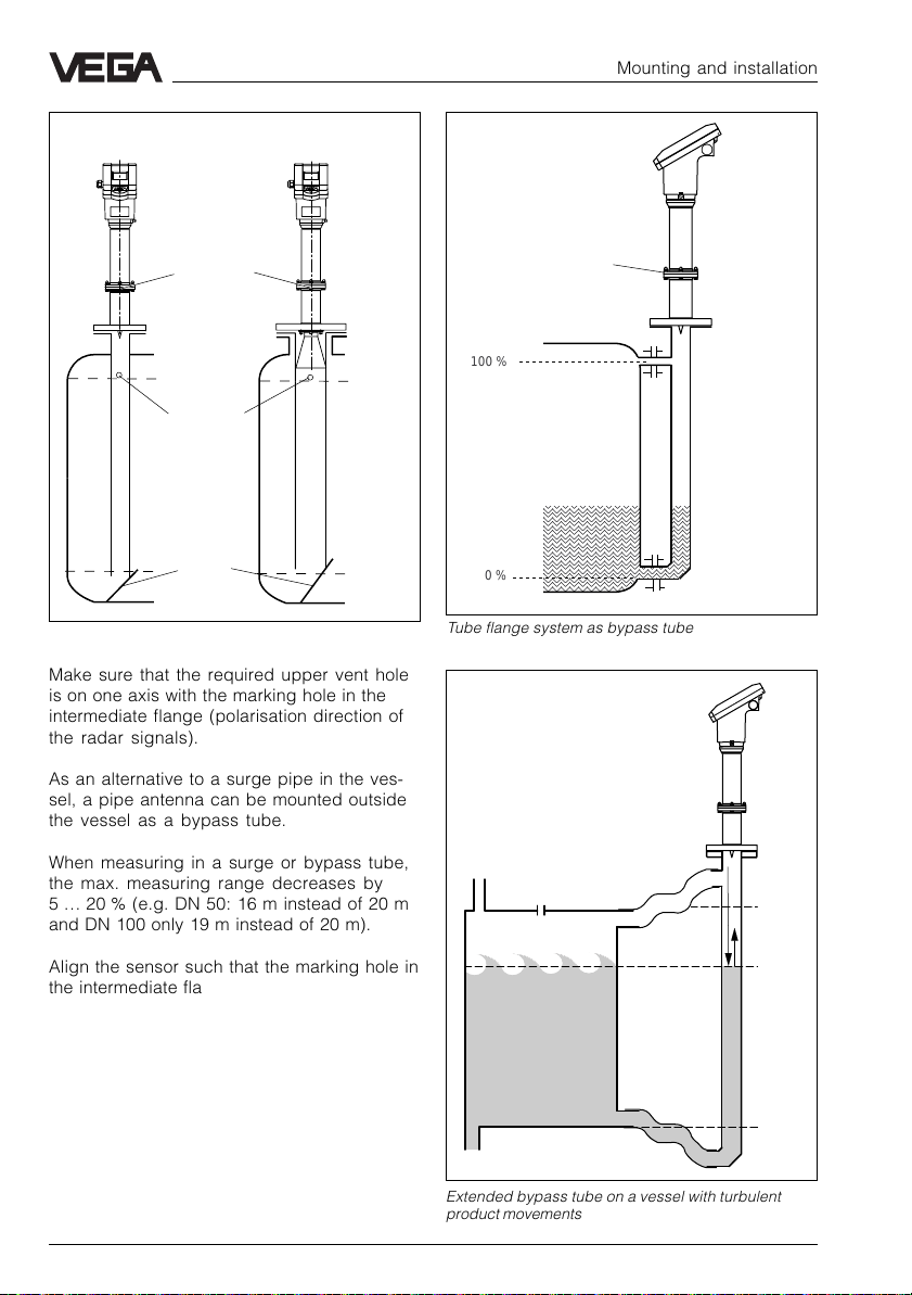
Make sure that the required upper vent hole is on one axis with the marking hole in the intermediate flange (polarisation direction of the radar signals).

Marking hole

100 %

;

0 %

Tube flange system as bypass tube

As an alternative to a surge pipe in the vessel, a pipe antenna can be mounted outside the vessel as a bypass tube.

When measuring in a surge or bypass tube, the max. measuring range decreases by 5 … 20 % (e.g. DN 50: 16 m instead of 20 m and DN 100 only 19 m instead of 20 m).

Align the sensor such that the marking hole in the intermediate flange is on one axis with the tube holes or tube openings. The polarisation of the radar signal enables a considerably stabler measurement with this alignment.

Extended bypass tube on a vessel with turbulent product movements

26 VEGAPULS 56 Profibus PA

100 %

75 %

0 %

Mounting and installation

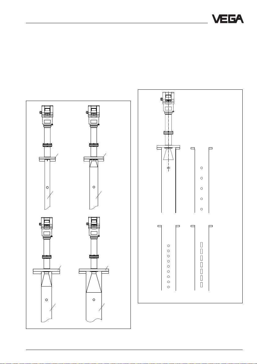
Adhesive products

For adhesive products, a surge pipe with a larger inner diameter should be used. For nonadhesive products, the best and most inexpensive solution is a measurement tube with a diameter of 50 mm. For slightly adhesive products, use a surge pipe with a nominal diameter of 100 mm to 150 mm to prevent buildup from causing measurement errors.

DN 50

ø 50

DN 80

ø 80

Standpipe measurement of inhomogeneous products

If you want to measure inhomogeneous products or stratified products in a surge pipe, it must have holes, elongated holes or slots. These openings ensure that the liquid is mixed and corresponds to the liquid in the vessel.

ø 100

DN 100

DN 150

ø 150

homogeneous liquids

inhomogeneous liquids

Openings in a surge pipe for mixing of inhomogene-

slightly inhomogeneous liquids

strongly inhomogeneous liquids

ous products

The more inhomogeneous the measured product, the closer together the openings

Pipe antenna with DN 50, DN 80, DN 100 and DN 150

VEGAPULS 56 Profibus PA 27

should be.

Mounting and installation

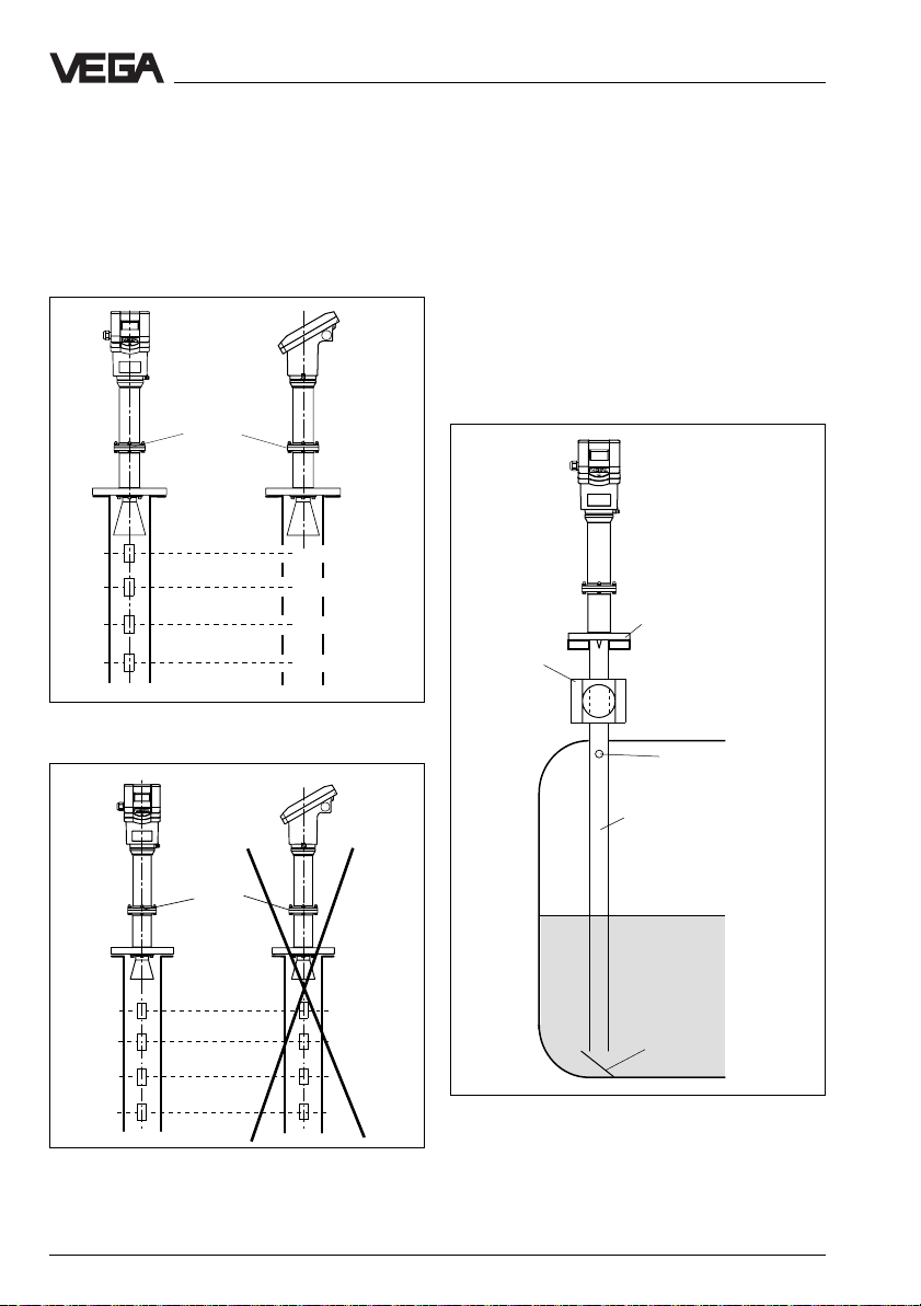
Polarisation direction

Due to radar polarisation, the holes or slots must be positioned in two rows offset by 180°. The radar sensor must be mounted so that the marking hole of the sensor (located in the intermediate flange) is on one axis with the row of holes in the standpipe.

Marking hole

Rows of holes in one axis with the marking hole

Surge pipe with ball valve

If a ball valve is mounted in the surge pipe, maintenance and servicing can be carried out without opening the vessel (e.g. if it contains liquid gas or toxic products).

A prerequisite for trouble-free operation is a ball valve throat that corresponds to the pipe diameter and provides a flush surface with the pipe inner wall.

Make sure there is a ventilation hole in the standpipe.

DN 50

Ball valve

Standpipe ventilation

Correct

Marking hole

The sensor must be directed with the marking hole to the rows of holes or openings.

28 VEGAPULS 56 Profibus PA

Wrong

ø50

Deflector

Tube antenna system with ball valve cutoff in measuring tube

Mounting and installation

In products with a small relative dielectric constant, a > 45° deflector plate installed under the end of the standpipe will prevent the vessel bottom from being detected as level instead of the product surface.

Vent hole

Pipe antenna systems must be provided with a vent hole at the upper end of the surge pipe. A missing hole will cause inaccurate measurements.

Correct

Pipe antenna: The surge pipe open to the bottom must have a vent or equalisation hole on top.

Wrong

VEGAPULS 56 Profibus PA 29

Guidelines for standpipe construction

Flange DN 50

100 %

Rz ≤ 30

Connection sleeves

Welding neck flanges

150…500

Welding neck flange

2,9…6

Welding of the connecting sleeve

5…15

0,0...0,4

Welding of the welding neck flange

2,9

1,5…2

Mounting and installation

Radar sensors for measurement on surge or bypass pipes are routinely mounted in flange sizes DN 50, DN 80, DN 100 and DN 150.

The illustration on the left shows the constructional features of a measuring pipe (surge or bypass tube) as exemplified by a sensor with DN 50 flange.

The radar sensor with a DN 50 flange only forms a functioning measuring system in conjunction with a measuring tube.

The measuring pipe must be smooth inside (average roughness Rz < 30). Use stainless steel tubing (drawn or welded lengthwise) for construction of the measuring pipe. Extend the measuring pipe to the required length with welding neck flanges or with connecting sleeves. Make sure that no shoulders or projections are created during welding. Before welding, join pipe and flange with their inner surfaces flush and exactly fitting.

Avoid welding through the pipe wall. The pipe must remain smooth inside. If the welding process inadvertently reaches the inner surface, any resulting roughness or welding beads must be carefully removed and burnished, as these cause false echoes and encourage product adhesion.

0,0…0,4

Deburr the holes

Deflector

0 %

ø 51,2

~45˚

Meas. pipe fastening

Min. product level to be measured (0 %)

Vessel bottom

30 VEGAPULS 56 Profibus PA

Mounting and installation

Flange DN 100

100 %

Deburr the holes

ø 96

Smooth welding neck flange

Welding of the plain welded flange

5…15

The illustration on the left shows the constructional features of a measuring pipe as exemplified by a sensor with DN 100 flange.

Radar sensors with flanges DN 80, DN 100 and DN 150 are equipped with a horn antenna. With these sensors, a plain welded flange can also be used on the sensor end instead of a welding neck flange.

If the vessel contains agitated products, fasten the measuring pipe to the vessel bottom. Provide additional fastenings for longer measuring pipes.

A deflector at the bottom end of the measuring pipe scatters the radar signals. In nearly empty vessels and products with low dielectric value, the deflector ensures that the product surface is detected rather than the vessel bottom. Products with low dielectric constants are partially penetrated, allowing the vessel bottom to produce (when the product level is low) a considerably stronger radar echo than the product surface.

150…500

0,0…0,4

With the deflector, however, only the useful signal is received in a nearly empty vessel the 0 % level is reliably detected and the correct measured value transmitted.

Connecting sleeve

Welding neck flanges

Rz ≤ 30

Deflector

0 %

ø 100,8

~45˚

VEGAPULS 56 Profibus PA 31

3,6

Welding of the welding neck flange

3,6

1,5…2

0,0…0,4

Meas. pipe fastening

Min. product level to be measured (0 %)

Vessel bottom

Mounting and installation

3.4 False echoes

The installation location of the radar sensor must be selected such that no installations or inflowing material cross the radar impulses. The following examples and instructions show the most frequent measuring problems and how to avoid them.

Vessel protrusions

Vessel forms with flat protrusions can, due to their strong false echoes, greatly affect the measurement. Shields above these flat protrusions scatter the false echoes and guarantee a reliable measurement.

Correct Wrong

Shield

Vessel protrusions (slope)

Intake pipes, i.e. for the mixing of materials with a flat surface directed towards the sensor - should be covered with a sloping shield that will scatter false echoes.

Vessel installations

Vessel installations such as, for example ladders, often cause false echoes. Make sure when planning your measuring location that the radar signals have free access to the measured product.

Correct Wrong

Ladder

Vessel installations

Ladder

Struts

Struts, like other vessel installations, can cause strong false echoes that are superimposed on the useful echoes. Small shields effectively hinder a direct false echo reflection. These false echoes are scattered and diffused in the area and are then filtered out as "echo noise“ by the measuring electronics.

Correct Wrong

Shields

Shield

Vessel protrusions (intake pipe)

32 VEGAPULS 56 Profibus PA

Struts

;;

;;;

;;

Mounting and installation

Strong product movements

Strong turbulence in the vessel, e.g. caused by stirrers or intense chemical reactions, can seriously interfere with the measurement. A surge or bypass tube (see illustration) of sufficient size always allows, provided that the product causes no buildup in the tube, a reliable measurement even with strong turbulence in the vessel.

Correct Wrong

100 %

75 %

0 %

Strong product movements

Products that cause only light buildup can be measured by using a tube with 100 mm nominal width or more. Light buildup in a tube of this size is no problem.

Buildup

If the sensor is mounted too close to the vessel wall, buildup and deposits from the measured product on the vessel wall cause false echoes. Position the sensor at a sufficient distance from the vessel wall. Please also note chapter "4.1 General installation instructions“.

Correct Wrong

Buildup

Inflowing material

Do not mount the instrument in or above the filling stream. Ensure that you detect the product surface and not the inflowing material.

Correct

Wrong

Inflowing material

VEGAPULS 56 Profibus PA 33

Mounting and installation

3.5 Installation mistakes

Socket piece too long

If the antenna is mounted in a socket extension that is too long, false reflections are caused, and measurement is hindered. Make sure that the horn antenna protrudes at least 10 mm out of the socket piece.

Correct Wrong

10 mm

Horn antenna: correct and wrong socket length

Wrong orientation to the product

A sensor orientation which does not point directly to the product surface causes weak measuring signals. Direct the sensor axis perpendicularly to the product surface to achieve optimum measuring results.

Parabolic effects on dished or arched vessel tops

Round or parabolic tank tops act like a parabolic mirror on the radar signals. If the radar sensor is placed at the focal point of such a parabolic tank top, the sensor receives amplified false echoes. The optimum mounting position is generally in the range of half the vessel radius from the centre.

Correct

>10 mm

vessel radius

Wrong

Correct Wrong

Wrong

Ladder

Direct sensor perpendicularly to the product surface

34 VEGAPULS 56 Profibus PA

Ladder

Mounting on a vessel with parabolic tank top

Mounting and installation

Standpipe (pipe antenna) without ventilation hole

Pipe antenna systems must be provided with a ventilation hole on the upper end of the pipe. If this hole is missing, incorrect measurements will result.

Correct Wrong

Pipe antenna: The surge pipe open to the bottom must have a ventilation hole on top

Wrong polarisation direction on the standpipe

When measuring in a surge pipe, especially if there are holes or slots for mixing in the tube, it is important that the radar sensor is aligned with the rows of holes.

The two rows of holes (displaced by 180°) of the measuring tube must be in one plane with the polarisation direction of the radar signals. The polarisation direction is always in the same plane as the marking hole. Precise directing is achieved by means of the marking holes in the intermediate flange.

Marking hole

The polarisation direction is in one plane with the marking hole (the sensor must be directed with the marking hole to the rows of holes).

Sensor too close to the vessel wall

If the radar sensor is mounted too close to the vessel wall, strong false echoes can be caused. Buildup, rivets, screws or weld joints superimpose their echoes onto the product or useful echo. Please ensure sufficient distance from the sensor to the vessel wall.

In case of good reflection conditions (liquids, no vessel installations), we recommend selecting the sensor distance such that there is no vessel wall within the inner emission cone.

For products with less favourable reflective properties, it is a good idea to also keep the outer emission cone free of interfering installations. Note chapter "4.1 General installation instructions“.

Foam generation

Thick, dense and creamy foam can cause incorrect measurements. Provide a means to prevent foam or measure in a bypass tube. Check, if necessary, the possibility of using a different measuring technology, e.g. capacitive electrodes or hydrostatic pressure transmitters.

VEGAPULS 56 Profibus PA 35

4 Electrical connection

4.1 Connection – Connection cable – Screening

Safety information – Qualified personnel

Instruments which are not operated with protective low voltage or DC voltage must be connected only by qualified personnel. This also applies to the configuration of measuring systems planned for Ex environment.

As a rule, do all connecting work in the complete absence of line voltage. Always switch off the power supply before you carry out connecting work on the radar sensors. Protect yourself and the instruments.

Connection cables and bus configuration

Note the Profibus specification. The connection cables must be specified for the expected operating temperatures in the plant and must have an outer diameter of 6 … 12 mm, to ensure sealing effect of the cable entry on the sensor.

For power supply and bus communication, a two-wire cable acc. to the Profibus specification (up to max. 2.5 mm of conductor) is used. The electrical connection on the sensor is made by spring-loaded terminals.

In a laboratory setup, a Profibus system will also work with standard, unshielded two-wire cable. In practice however, an automation network and bus system can only be protected reliably against electromagnetic interference with screened cable. Acc. to the Profibus specification (IEC 1158-2), screened and twisted cables are prescribed. All participants are connected in one line

cross-section area

Electrical connection

(serially). At the beginning and end of the bus segment, the bus is terminated by an active bus termination. On the DP bus level, most participants already have a bus termination implemented. With more than 32 participants on the DP level, a so-called repeater must be used to open and combine another DP level with a max. of 32 additional participants. On the PA bus branch of the segment coupler, the PA radar sensors work also with max. 32 participants (Ex max. 10 participants).

A PA sensor can work only in conjunction with a Profibus DP system, to which a Profibus PA subsystem is connected. A PA Profibus participant must consume min. 10 mA supply current.

Connection cable and cable length

Connection cables must correspond to the Profibus specification and the FISCO model. The sensor cable must be in conformity with the values of the reference cable acc. to IEC 1158-2:

0.8 mm Z C

The max. cable length first of all depends on the transmission speed: up to 32 kbit/s: 1900 m Prup to 32 kbit/s: 1900 m Pr

up to 32 kbit/s: 1900 m Pr

up to 32 kbit/s: 1900 m Prup to 32 kbit/s: 1900 m Pr up to 94 kbit/s: 1200 m Profibus DP up to 188 kbit/s: 1000 m Profibus DP up to 500 kbit/s: 500 m Profibus DP up to 1500 kbit/s: 200 m Profibus DP up to 12000 kbit/s: 100 m Profibus DP

The distributed resistance of the cable, in

; R

= 44 Ω/km;

DCmax.

= 80 … 120 Ω; damping = 3 dB/km;

31.25kHz

= 2 nF/km.

asymmetric

ofibus Pofibus P

ofibus P

ofibus Pofibus P

36 VEGAPULS 56 Profibus PA

Electrical connection

conjunction with the output voltage of the segment coupler and the current requirement (VEGAPULS 10 mA) or the voltage requirement (VEGAPULS 9 V) of the sensors, determines the max. length of the cable.

In a practical application of a PA bus branch, the max. length of the cable is also determined (beside the required supply voltage and max. current consumption of all participants on the PA bus branch) by the bus structure and the type of segment coupler used.

The cable length results from the sum of all cable sections and the length of all stubs. The length of the individual stubs must not exceed the following lengths: 1 … 12 stubs 120 m (Ex: 30 m) 13 … 18 stubs 60 m (Ex: 30 m) 19 … 24 stubs 30 m (Ex: 30 m)

More than 24 stubs are not permitted, whereby each branch longer than 1.2 m is counted as a stub. The total length of the cable must not exceed 1900 m (in Ex version 1000 m).

Ground terminal

The electronics housings of the sensors have a protective insulation. The ground terminal in the electronics is galvanically connected with the metallic process connection. For sensors with a plastic thread as process fitting, the sensor grounding must be made by a ground connection to the outer ground terminal.

Screening

"Electromagnetic pollution“ caused by electronic actuators, energy cables and transmitting systems has become so pervasive that shielding for normal two-wire bus cable is usually a necessity. According to the Profibus specification, the screen should be grounded on both ends. To avoid potential equalisation currents, a potential equalisation system must be provided in addition to the screening.

According to specification, we recommend the use of twisted and screened two-wire cable, e.g.: SINEC 6XV1 830-5AH10 (Siemens), SINEC L26XV1 830-35H10 (Siemens), 3079A (Belden).

Alternatively, when grounding at both ends in non-Ex areas, the cable shielding can be connected on one ground side (in the switching cabinet) via an Y 1500 V) to the ground potential. Make sure

-capacitor (e.g. 10 nF,

that the ground connection has the lowest possible resistance (foundation, plate or mains earth).

Profibus PA in Ex environment

When used in Ex area, a PA bus with all connected instruments must be carried out in intrinsically safe protection class "i“. Four-wire instruments requiring separate supply must at least have an intrinsically safe PA connection. VEGA sensors for PA-Ex environment are generally "ia” two-wire instruments.

VEGAPULS 56 Profibus PA 37

Electrical connection

In the so-called Fieldbus Intrinsically Safe Concept (FISCO), the general conditions for an Ex safe bus configuration have been laid down. Therein, the participants and the bus cables with their electrical data have been determined, so that the linking of these components always meets Ex requirements. A more time-consuming Ex calculation is therefore not necessary. You can build your Ex bus according to the IEC standard 1158-2.

The Ex segment coupler delivers a controlled power supply to the PA bus. It acts as source in the PA branch. All other components (field instruments and bus terminators) are only consumers. A field instrument must consume at least 10 mA. Ideally, an individual sensor should not consume more than 10 mA, so that the number of instruments can be as large as possible.

VEGA PA sensors, whether Ex or non Ex, consume a constant current of 10 mA. According to the Profibus specification, this is the minimum participant current. With VEGA sensors it is therefore possible to connect 10 sensors (also in Ex environment) even with a limited energy supply from the Ex segment couplers.

Watch out for potential losses

Due to potential losses, earthing on both ends without a potential equalisation system is not allowed in Ex applications. If an instrument is used in hazardous areas, the required regulations, conformity and type approval certificates for systems in Ex areas must be noted (e.g. DIN 0165). Please also note the approval documents with the safety data sheet attached to the Ex sensors.

Electrical data of the cables

No. of A in Z cores mm

31.25kHz

C in Damping Screen nF/km

SINEC 6XV1 44 Ω/km 2 0.75 100 Ω < 90 < 3 dB/km Cu braiding 830-5AH10 +/- 20 Ω 39 kHz (Siemens)

SINEC L26XV1 44 Ω/km 2 0.75 100 Ω < 90 < 3 dB/km Cu braiding 830-35H10 +/- 20 Ω 39 kHz (Siemens)

3079A 105 Ω/km 2 0.32 150 Ω 29.5 < 3 dB/km Foil (Belden) 39 kHz

38 VEGAPULS 56 Profibus PA

Electrical connection

4.2 Sensor address

In a Profibus system composed of Profibus DP and Profibus PA subsystem, each participant must have a unique address. Each participant, whether master or slave, is accessed by means of its own address in the bus system. The address of a participant, whether on DP or PA level, should be assigned before connecting to the bus, because an address can be used only once. If an address is used twice, interference in the bus will be caused.

The address of a radar sensor can be set in two ways:

- with the adjustment software VVO (software addressing) or

- with the DIP switch block in the sensor (hardware addressing).

VEGA Profibus sensors are delivered with the address set at 126 (all DIP switches to "ON“). Remember, in a Profibus system there are max. 126 participants possible. When the DIP switch is set to address 126 (or higher), the address can be adjusted with the adjustment software VVO, the adjustment module MINICOM or another configuration tool (e.g. PDM). However, there can be only one sensor on the bus with address 126 (delivery status) during address assignment via software. For that reason, hardware addressing (DIP switch) before connection to the bus is recommended.

Hardware addressing

The DIP switches generate an address number in the binary system. This means that, from right to left (ascending), any switch represents a number twice as high as the previous switch on the right. The corresponding number in the decimal system results from the sum of all switches set to "ON“. In the illustration you see the decimal number that corresponds to each individual DIP switch.

DIP switch 8 corresponds to the number 128, switch 1 corresponds to the number 1 and switch 3 corresponds to the decimal number

8765 4

128

Example 1

The switches 3, 5 and 7 are set to "ON“. The address is then: DIP switch 3 to "ON“ means 4 DIP switch 5 to "ON“ means 16 DIP switch 7 to "ON“ means 64

The sum is: 4 + 16 + 64 = Address 84

8765 4

64 + 16 + 4 = 84

VEGAPULS 56 Profibus PA 39

Electrical connection

Example 2

You want to set address 27. 16 + 8 + 2 + 1 = 27

You must set the DIP switches 5 = 16 4 = 8 2 = 2 1 = 1 to "ON“.

Example 3

You want to set address 99 64 + 32 + 2 + 1 = 99

You must set the DIP switches 7 = 64 6 = 32 2 = 2 1 = 1 to "ON“.

Software addressing

The DIP switches must be set to an address of 126 … 255, i.e.

- either all DIP switches are set to "ON“, corresponding to address 255 (delivery status)

OFF

8765 4

Addr.

- or only DIP switch 8 is set to "ON“, corresponding to address 128.

The adjustment of the address with software VVO is described in chapter "5.2 Adjustment with VVO“ under the heading "Software addressing“ or in chapter "5.3 Sensor adjustment with the adjustment module MINICOM“.

128

8765 4

4.3 Connection of the sensor

After mounting the sensor at the measurement location according to the instructions in chapter "3 Mounting and installation“, loosen the closing screws on top of the sensor. The sensor lid with the optional indication display can then be opened. Unscrew the sleeve nut and slip it over the connection cable (after removing about 10 cm of insulation). The sleeve nut of the cable entry has a self-locking ratchet that prevents it from opening on its own.

Now insert the cable through the cable entry into the sensor. Screw the sleeve nut back onto the cable entry and clamp the stripped wires of the cable into the proper terminal positions.

The terminals hold the wire without a screw (spring-loaded terminals). Press the white opening tabs with a small screwdriver and insert the copper core of the connection cable into the terminal opening. Check the hold of the individual wires in the terminals by lightly pulling on them.

Of course, software addressing is also possible, if the switches 7 … 2 are set to "ON“ (address 126).

40 VEGAPULS 56 Profibus PA

ESC

Electrical connection

Ex ia version

Power supply and digital measuring signal

To the indicating instrument in the

sensor lid or to the external indicating instrument VEGADIS 50

M20x1.5 (diameter of the connection cable 6…9 mm)

Spring-loaded terminals (max. 2.5 mm section)

wire cross-

12 C 567843

12 C 5 6 7 843

Commu-

VBUS

nication+-4...20mA

Spring-loaded terminals (max. 2.5 mm section)

Display

ESC

Sockets for connection of VEGACONNECT 2 (communication sockets)

wire cross-

Exd version (loop-powered with pressure-tight encapsulated terminal compartment)

EEx d connection housing

(opening in Ex area not allowed)

Power supply and digital measuring signal

Locking of the cover

Supply: 20 … 36 V DC, VBUS

Shield

- +

Exd terminal compartment

/2“ NPT EEx d diameter of the connection cable

3.1…8.7 mm (0.12…0.34 inch)

Adjustment module and terminal compartment of display

(opening in Ex area permitted)

Exd safe connection to the Exd terminal compartment

/2“ NPT EEx d diameter of the connection cable to the Exd terminal compartment

3.1…8.7 mm (0.12…0.34 inch)

12 C 567843

12 C 5 6 7 843

Commu-

VBUS

nication+-4...20mA

Display

ESC

VEGAPULS 56 Profibus PA 41

ESC

Tank 1 m (d)

12.345

Electrical connection

4.4 Connection of the external indicating instrument VEGADIS 50

Loosen the four screws of the housing lid on VEGADIS 50. The connection procedure can be facilitated by fixing the housing cover during connection work with one or two screws on the right of the housing (figure).

Input of the sensor

SENSOR

Power supply

DISPLAY (in the lid of the indicating instrument)

DISPLAY1234 56 78

Terminal strip in VEGADIS 50

M20 x 1.5 (diameter of the connection cable 5…9 mm)

Note:

The four-wire connection cable to VEGADIS 50 should be screened and have a max. length of 25 m. The digital signals to the indicating instruments would otherwise be impaired by the cable capacitance of longer connection cables. Ground the cable screen together with the signal cable screen on the sensor.

VEGADIS 50

Adjustment module

Screws

12 C 567843

12 C 5 6 7 843

Commu-

VBUS

nication+-4...20mA

Display

ESC

42 VEGAPULS 56 Profibus PA

Setup

5 Setup

5.1 Adjustment media

In chapter "1.4 Adjustment“ the Profibus adjustment structure was briefly explained and the adjustment media for VEGA Profibus sensors were shown. All VEGA Profibus sensors operate in profile 3 and can be adjusted with:

- the adjustment program VVO on a PC with Profibus card

- the adjustment program PACTware which VVO runs as a subprogram

- the Siemens software PDM in conjunction with an EDD (Electronic-Device-Description)

- the adjustment module MINICOM in the sensor.

Adjustment with VVO on the PC

The adjustment program VVO enables userfriendly adjustment of VEGA Profibus PA sensors. All functions and options of sensor adjustment are accessible. The program runs under Windows Profibus-Master-Class 2 inter face card on Profibus DP level as Master-Class 2 tool. The VVO program accesses the VEGA PA sensors via the DP bus, the segment coupler and the PA bus.

on a PC with a

, under

Adjustment with PACTware

The adjustment with PACTwareTM corresponds to VVO adjustment, in this case, VVO runs as a subprogram of PACTware adjustment instructions can be found in the documentation of PACTware

. The

Adjustment with PDM

The sensors can be adjusted completely with PDM. However, some convenient functions and many special features, like e.g. display of an echo curve, are not available. In addition to the PDM software, an EDD (upon request available from VEGA) is required for each sensor type. The adjustment instructions for PDM are described in the PDM documentation.

Adjustment with the adjustment module MINICOM

With the adjustment module MINICOM, you adjust the individual sensor directly in the sensor or in the external indicating instrument VEGADIS 50. The adjustment module MINICOM enables (with the 6-key adjustment field with text display) all essential functions of parameter setting and adjustment.

Note:

Keep in mind that for adjustment with VVO, version 2.70 or higher is necessary.

VEGAPULS 56 Profibus PA 43

Setup

5.2 Adjustment with VV O

Before you can adjust the sensors with the adjustment program VVO (VEGA Visual Operating) in version ≥ 2.70, they must be integrated into the Profibus system. First of all, address the sensors (chapter "4.2 Sensor address“) and connect them to your PA segment. With the attached GSD file you integrate the sensors into your system.

To adjust VEGA sensors with the adjustment software VVO, the PC or the adjustment station on which VVO is installed must be equipped with a Profibus DP interface card (e.g. of Messrs. Softing). The PC or the adjustment station communicates then as Master-Class 2 participant on the DP bus with the VEGA sensors on the PA bus segment.

To connect the PC to the DP bus, a standard RS 485-DTE interface cable (Data Terminal Equipment) is required. With the cable you connect the DP interface card to the bus or to the segment coupler.

PCPC

Screen 1 1 Screen – – 2 2 M24 RxD/TxD-PRxD/TxD-P

RxD/TxD-P

RxD/TxD-PRxD/TxD-P

33 – – 4 4 CNTR-P GNDGND

GND

GNDGND

55 – – 6 6 VP – – 7 7 P24 RxD/TxD-NRxD/TxD-N

RxD/TxD-N

RxD/TxD-NRxD/TxD-N

88 – – 9 9 CNTR-P

Profibus-DP DP bus (in brackets the interface card PIN number of the P+F

BUSBUS

BUS

BUSBUS

RxD/TxD-PRxD/TxD-P

RxD/TxD-P (40)

RxD/TxD-PRxD/TxD-P

GNDGND

GND (55)

GNDGND

RxD/TxD-NRxD/TxD-N

RxD/TxD-N (41)

RxD/TxD-NRxD/TxD-N

segment couplers)

Segment coupler

DP cable

VVO

VEGACONNECT 3

Profibus DP interface card (Messrs. Softing)

Sensor Sensor Sensor Sensor

Profibus PA cable

When the computer is connected to the Profibus DP cable, you can start VVO.

In the following setup and adjustment instructions you will find information on the following topics and adjustment items:

ConfigurationConfiguration

•

Configuration

ConfigurationConfiguration

- Configuration info

- Software addressing

- Create new measurement loop Parameter adjustment 1Parameter adjustment 1

•

Parameter adjustment 1

Parameter adjustment 1Parameter adjustment 1

- Meas. loop data

- Adjustment

- Scaling Sensor optimisationSensor optimisation

•

Sensor optimisation

Sensor optimisationSensor optimisation

- Meas. environment/Operating range

- Meas. environment/Meas. conditions

- Meas. environment/Sonic velocity

- Echo curve

- False echo storage Parameter adjustment 2Parameter adjustment 2

•

Parameter adjustment 2 (optional)

Parameter adjustment 2Parameter adjustment 2

- Linearisation

- Defining the linearisation curve by incremental filling

- Calculating the linearisation curve

- Calculate cylindrical tank

- Parameter adjustment sensor display

• Display measured value

• Simulation

• Print configuration and adjustments

• Backup

44 VEGAPULS 56 Profibus PA

Setup

Configuration and parameter adjustment

During setup of the sensor you will be confronted with two terms: "Configuration“ and "Parameter adjustment“. The meas. system is first set up with a configuration and then with a parameter adjustment.

Configuration

The term "Configuration“ means the basic adjustments of the meas. system. You inform the meas. system about the application (level measurement, gauge, distance …), the measurement loop name and the DCS output address of the sensors. The configuration corresponds to an electronic wiring and labelling of your sensor or, in other words, telling the system which sensor for what application and where.

Parameter adjustment

After the configuration, you carry out the parameter adjustment for each individual sensor. This means adjusting the sensors to the respective operating range and to the actual application. You inform the sensor which product distance (which level) is "empty“ and which "full“. This is called adjustment. Here you choose in which physical quantity (volume, mass) and unit of measurement (m ured value should be outputted. In the submenu "Sensor optimisation“ you inform the sensor electronics about the actual environment, such as e.g. quick changes of the measured value, foam generation, gas stratification, solid or liquid state of the medium.

, gal, liters …) the adjusted meas-

Actions, like entering a value or making a choice, are indicated in the following by a large black dot, like this:

• Choose …

• Start …

• Click to …

By this convention, the actions to be carried out are clearly separated from supplementary information in the following adjustment instructions.

Note:

By default, the adjustment software VVO uses address 10 when operating via the PA interface card on the PA bus as Master-Class

2. If on your bus address 10 is already assigned, enter a free address (description on the next page) before connecting the PC to the bus.

• Now start the adjustment software VVO on your PC.

• Choose with the arrow keys or the mouse the item "Planning“ on the entrance screen and click to "

OKOK

“.

You are asked for user identification.

Before starting the setup:

Do not be confused by the many pictures, adjustment steps and menus on the following pages. Just carry out the setup with the PC step by step and you will soon no longer need the following pages.

VEGAPULS 56 Profibus PA 45

• Enter under name "

• Also enter "

VEGAVEGA

VEGA“.

VEGAVEGA

VEGA“ under password.

VEGAVEGA

The adjustment program, called in the following VVO, gets into contact with the connected sensor …

Setup

… and asks in which mode the adjustment software should be used. After a few seconds, the software indicates if and with which system a connection exists.

If the following message is displayed, you have to change the communication setting in VVO.

• Then click to "

gramgram

gram

“ and click to "

gramgram

ConfigurationConfiguration

Configuration

ConfigurationConfiguration

CommunicationCommunication

Communication

CommunicationCommunication

“, point to "

Pro-Pro-

Pro-

Pro-Pro-

“.

• Click to "

The window for the bus communication settings opens. 10 is preset as the address for the Master Class 2 interface card. If participant number ten is free on your bus, you can accept the setting. Typical values for bus parameters have been preset. At this point, you should set the communication parameters that apply to your system.

• Now click to "

The message "

dows

Bus parametersBus parameters

Bus parameters

Bus parametersBus parameters

OKOK

“.

OKOK

must be restarted

VVO will shut down and Win-

“.

“ appears.

Note: As a rule, a Windows® restart is not

PrPr

• First click to " Then choose the Profibus card which is installed in your PC.

46 VEGAPULS 56 Profibus PA

ofibus DP (for Pofibus DP (for P

ofibus DP (for P

PrPr

ofibus DP (for Pofibus DP (for P

A sensorsA sensors

A sensors

A sensorsA sensors

necessary.

“.

• Now start VVO (restart).

Setup

• Click to "

The VVO software asks again for the user identification and then reads in all VEGA Profibus sensors found. You now see the VVO main menu window.

User identification

The preset user identification can be modified at a later time in the menu "

Program/User access

PlanningPlanning

Planning

PlanningPlanning

“ and then to "

“.

OKOK

“.

OKOK

Configuration/

Configuration

Configuration info

• Choose the menu "

ing systeming system

ing system

ing systeming system

You reach the menu window "

measuring system

complete information on the VEGA sensors connected to the Profibus.

Software addressing

If the DIP switch in the sensor is set to address 126 or higher, the address can be modified in the menu window "

measuring system

the field "

Sensor address

Configuration/MeasurConfiguration/Measur

Configuration/Measur

Configuration/MeasurConfiguration/Measur

“.

Configuration

“. In this window you get

Configuration

“. Enter a free address in

“.

VEGAPULS 56 Profibus PA 47

Setup

The measurement loops are listed in the sequence of sensor addresses with a serial number and any existing name.

If the sensor address has been adjusted with the DIP switch from 1 … 125, the address number in the field " and cannot be changed at this point.

Create new measurement loop

• Choose the menu "C

ment loop/Modify

Sensor address

onfiguration/Measure-

“.

“ is grey

• Choose in the window "

configuration

name for the measurement loop.

“ the application and enter a

Modify meas. loop

Parameter adjustment 1

In the menu "

justment

adjustments.

Instrument data/Parameter ad-

“ you carry out all important sensor

The menu window "

loop - Modify meas. loop configuration

opens.

• Here you choose the sensor to be configured.

48 VEGAPULS 56 Profibus PA

Selection of measurement

“

• Choose the menu "

eter adjustmenteter adjustment

eter adjustment

eter adjustmenteter adjustment

which you want to carry out the parameter adjustment.

In the opening menu window, you now see the measurement loop names and descriptions previously entered under "

measurement loop

configured or connected one sensor, there will naturally be a choice of only one sensor.

Instrument data/Param-Instrument data/Param-

Instrument data/Param-

Instrument data/Param-Instrument data/Param-

“ and then the sensor on

Create new

“. If you have only

Setup

• Click to the sensor or the measurement loop on which you want to carry out the parameter adjustment.

• Then click to "

strument data parameter adjustment

opens.

OKOK

“, the menu window "

OKOK

“

Adjustment

("adjustment“ in chapter "6 Function diagram).

In-

Measurement loop data

• When clicking " important measurement loop data will be displayed.

Meas. loop dataMeas. loop data

Meas. loop data

Meas. loop dataMeas. loop data

“, the most

• Click to "

• Click in the menu window " "

You can carr y out the min./max. adjustment

"with medium“

real level) or the real level into account, i.e. with empty vessel).

Generally, you will carry out the adjustment without medium, so you are completely independent of the actual vessel filling during the adjustment. If you want to carry out the adjustment with medium, you have to carry out the min. adjustment with emptied (also partly emptied) vessel and the max. adjustment with filled vessel (also partly filled vessel). It is therefore easier and faster to carry out the adjustment without medium.

AdjustmentAdjustment

Adjustment

AdjustmentAdjustment

Min/Max-AdjustmentMin/Max-Adjustment

Min/Max-Adjustment

Min/Max-AdjustmentMin/Max-Adjustment

(adjustment by means of the

"without medium“

“.

Adjustment

(without taking

“ to

• Click to " menu window "

adjustment

VEGAPULS 56 Profibus PA 49

QuitQuit

Quit

“ and you are again in the

QuitQuit

Instrument data parameter

“.

Setup

no (adjustment without medium)no (adjustment without medium)

• Choose "

In the menu window "Min/Max-Adjustment“ you choose e.g. the level distance corresponding to 100 % and 0 %. Of course, you can also enter the distance values e.g. at 20 % and 75 % filling.

If the two points are too close together, e.g. at 45 % and 49 %, a considerable meas. error can result, as the sensor generates by means of the two adjustment points a linear correlation between filling volume (%) and meas. distance.

no (adjustment without medium)

no (adjustment without medium)no (adjustment without medium)

• Confirm the adjustments with "

“.

after a message is displayed, you are again in the menu window "

Note:

The sensor is delivered with the sensor measuring range set to the same value as the operating range. After the sensor has been adjusted, the operating range corresponds to the adjustment range. The sensor can only detect levels within the defined operating range. For level detection outside the operating range (if you want to detect e.g. 108 % and -10 %), the operating range must be corrected respectively in the menu "

OKOK

Adjustment

sor optimisation/Meas. environment

following chapter "Sensor optimisation“, "Meas. environment/Operating range“).

• Click in the menu window "

QuitQuit

Quit

“.

QuitQuit

Adjustment

“ and

“.

Sen-

“ (see the

“ to

• Choose if you want to carry out the adjustment in

meters

• Enter a distance for the upper and lower

(m) or in

level and the extent of filling in % corresponding to each distance.

In the example, the 0 % filling is at a product distance of 5.850 m and the 100 % filling at a product distance of 1.270 m.

Offset

See also A3-1 in chapter "6 Function diagram“ under "Level Offset“.

50 VEGAPULS 56 Profibus PA

feet

(ft).

You are again in the menu window "

ment data parameter adjustment

“.

Instru-

Setup

The sensor electronics has two characteristics points (at min. and max.) from which a linear proportionality between product distance and the percentage of filling of the vessel is generated. Of course, the characteristics points must not necessarily be at 0 % and 100 %, however they should be as far apart as possible (e.g. at 20 % and at 80 %). The difference between the characteristics points for the min./ max. adjustment should be at least 20 mm product distance. If the characteristics points are too close together, the possible measuring error increases. Ideally, the adjustment would be to carried out, as shown in the example, at 0 % and at 100 %.

In the menu "

justment/Conditioning/Linearisation

enter later, if necessary, a correlation between product distance and % extent of filling other than linear (see later subitem Linearisation).

Scaling

• Click in the menu window "

parameter adjustment

Instrument data/Parameter ad-

“ you can

Instrument data

ConditioningConditioning

“ to "

Conditioning

ConditioningConditioning

“.

ScalingScaling

Scaling

ScalingScaling

Outputs

“.

“ in the menu window

OKOK

“.

OKOK

Conditioning

“.

“ to

Instru-

• Click to "

The displayed message tells you that you will find this function on Profibus sensors under the menu item " "

Instrument data parameter adjustment

• Confirm the message with "

• Click in the menu window "

QuitQuit

Quit

QuitQuit

You are again in the menu window "

ment data parameter adjustment

Scaling of the output signal

• Click in the menu window "

parameter adjustment

The menu window "

VEGAPULS 56 Profibus PA 51

Conditioning

“ opens.

Instrument data

OutputsOutputs

“ to "

Outputs

OutputsOutputs

“.

Setup

Profibus outputProfibus output

• Click to "

In the window " determine the options for the Profibus output (acc. to the Profibus PA instrument profile).

VEGA Profibus sensors operate in the socalled profile 3, in which the structure of measured value processing is determined (see also chapter "6 PA Function diagram“). In this software diagram you can see the structure of the measured value processing acc. to profile 3 (schematic presentation). The numberings A1, A2 … E are also stated in the PA function diagram.

PV-Scale

Profibus output

Profibus outputProfibus output

Profibus output

Out-Scale

“.

“ you can

You can choose as a physical quantity

"dimensionless mass, height and distance“

appropriate unit of measurement (e.g. l, hl). The sensor display then shows the measured value in the selected physical quantity and unit.

• Save the adjustments in the menu "

output

The adjustments are now transferred to the sensor and you are again in the menu window "

Outputs

• Click in the menu window "

QuitQuit

Quit

QuitQuit

• Click in the menu window "

parameter adjustment

(plain numbers),

OKOK

“ with "

OKOK

“.

volume,

and assign an

Profibus

“.

Outputs

“ to

Instrument data QuitQuit

“ to "

Quit

“.

QuitQuit

52 VEGAPULS 56 Profibus PA

Setup

Sensor optimisation

In the menu " pare the sensor for the meas. environment. With this you can carry out special optimising adjustments, and optimise, e.g., the mounting locating of the sensor by means of an echo curve.

Meas. environment/Operating range

• Choose the menu "

eter adjustmenteter adjustment

eter adjustment

eter adjustmenteter adjustment

• Choose in the menu window "

data parameter adjustmentdata parameter adjustment

data parameter adjustment

data parameter adjustmentdata parameter adjustment

Sensor optimisationSensor optimisation

Sensor optimisation

Sensor optimisationSensor optimisation

Sensor optimisation

Instrument data param-Instrument data param-

Instrument data param-

Instrument data param-Instrument data param-

“ and then the sensor.

“ the menu item

““

“.

““

“ you pre-

InstrumentInstrument

Instrument

InstrumentInstrument

The window "

With the menu item " can define a sensor operating range that deviates from the meas. range (depending on the sensor type) and from the "

adjustment

corresponds otherwise to the min./max. adjustment (span), i.e. the meas. range.

Meas. environment

Operating range

“ opens.

“ you

Min/Max

“. By default, the operating range

Generally, it is better to set the operating range approx. 5 % wider than the adjusted measuring range (span) determined by the min./max. adjustment. In the example:

- Min. adjustment to 1.270 m,

- Max. adjustment to 5.85 m. In the example you would have set the operating range from 1 m to 6 m.

• First click to

VEGAPULS 56 Profibus PA 53

Meas. environmentMeas. environment

Meas. environment

Meas. environmentMeas. environment

““

“.

““

Meas. conditions/Pulse velocity

Setup

• Save the adjustments with " are again in the menu window "

ronment

“.

OKOK

“ and you

OKOK

Meas. envi-

Meas. environment/Meas. conditions

• Click in the menu window "

mentment

ment

mentment

• In the menu window " click on the options corresponding to your application.

• Confirm with

Meas. conditionMeas. condition

“ to "

Meas. condition

Meas. conditionMeas. condition

OKOK

““

“.

““

Meas. environ-Meas. environ-

Meas. environ-

Meas. environ-Meas. environ-

“.

Meas. conditions

“ you

In the menu item " are only necessary when measuring in a surge or bypass tube (standpipe). When measuring in a standpipe, a shift of the running time of the radar signal is caused which is dependent on the inner diameter of the standpipe. To take this running time shift into account, it is necessary to inform the sensor in this menu about the diameter (inner) of the standpipe.

Pulse velocity

“, adjustments

After a few seconds, during which the adjustments are permanently saved in the sensor, you are again in the window "

ment

“.

54 VEGAPULS 56 Profibus PA

Meas. environ-

• With "

• Click in the window "

sensor.

QuitQuit

Quit

“.

QuitQuit

OKOK

“ you save the adjustments in the

OKOK

Meas. environment

“ to

Setup

Echo curve

With the menu item " window "Sensor optimisation“ you can see the course and the strength of the detected radar echo. If, due to vessel installations, you expect strong false echoes, a correction (if possible) of the mounting location and orientation (during simultaneous monitoring of the echo curve) can help localise and reduce the size of the false echoes.

Echo curve

“ in the menu

In the next illustration, you see the echo curve after optimum orientation of the sensor to the product surface (sensor axis perpendicular to the product surface). The false echo, e.g. caused by a strut, is now reduced by more than 10 dB and will no longer influence the measurement.

• Quit the menu "

False echo storage

With the menu item " the menu " thorise the sensor to save false echoes. The sensor electronics then saves the false ech-

In the following illustration, you see the echo curve with a false echo nearly as large as the product echo (before correcting the sensor orientation, i.e. pointing the sensor directly at the product surface).

oes in an internal database and assigns them a lower level of importance than the useful echo. Carry out the false echo storage with the vessel emptied.

• Click in the menu window to "

optimisation storagestorage

storage

storagestorage

VEGAPULS 56 Profibus PA 55

Echo curve

False echo storage

Sensor optimisation

“ to the menu item

““

“.

““

QuitQuit

“ with "

Quit

QuitQuit

“ you can au-

Sensor

False echoFalse echo

False echo

False echoFalse echo

“.

“ in

• Click to

Show echo curveShow echo curve

Show echo curve

Show echo curveShow echo curve

Setup

““

“.

““

• Now click in the opening menu window "

False echo storage

oesoes

““

oes

“. A small window opens.

oesoes

““

• Enter here the verified product distance or the distance to the vessel bottom and click

Create newCreate new

Create new

Create newCreate new

You hereby authorise the sensor to mark all echoes before the product echo as false echoes. This prevents the sensor from erroneously detecting a false echo as level echo.

“.“.

“.

“.“.

Learn false ech-Learn false ech-

“ to

Learn false ech-

Learn false ech-Learn false ech-

The false echo marking and the real echo curve (top) are shown.

QuitQuit

• Quit the menu with

You are again in the menu window "

optimisation

reset all options of the menu "

optimisation

• Quit the menu window "

optimisation

You are then in the initial menu window "

“. With the menu item "

“ to default.

“ with

strument data parameter adjustment

Quit

QuitQuit

Quit

QuitQuit

““

“.

““

Sensor

““

“.

““

Sensor

Reset

Sensor

“.

“ you

In-

56 VEGAPULS 56 Profibus PA

Setup

Parameter adjustment 2

Linearisation

The relation between level and volume is defined with so-called linearisation curves. If there is a correlation in your vessel between level ("

Percentage value

quantity (value of the volume) other than linear, choose the menu window "

ing

“.

“ of the level) and

Condition-

Beside the two programmed linearisation curves "

Cylindrical tank

you can also enter "

curves

“. Linear means that there is a linear

correlation between level and volume.

User programmable linearisation curves

“ and "

Spherical tank

user programmable

“

• Click to " enter your own vessel geometry or a user programmable filling curve.

• Click to "

• Click in the menu window " the menu item

The menu window " which a linear correlation between percentage value of the level and the percentage value of the volume is preset.

VEGAPULS 56 Profibus PA 57

LinearisationLinearisation

Linearisation

LinearisationLinearisation

Linearisation

Conditioning

““

“.

““

“ opens, in

“ to

User programmable curveUser programmable curve

User programmable curve

User programmable curveUser programmable curve

EditEdit

Edit

“.

EditEdit

“

The user programmable linearisation curve is generated by index markers. Each index marker consists of a value pair. A value pair is generated from a value " value "

Percentage value

Linearised

“.

“Percentage value”

“ and a

represents the distance as a percentage of the level. "

Linearised

“ represents the percentage of vessel volume at a certain percentage value of level.

In the field "

Transfer measured value

“ the current level as a percentage of the adjusted span is displayed. The measuring window has already been adjusted with the min./max. adjustment. In the example, the span is

4.58 m and is between 5.85 m (empty) and

1.27 m (full), see the following illustration.

Setup

5.85 m meas. distance correspond to 0 % level. 1.27 m meas. distance correspond to 100 % level. The span is therefore 4.58 m (5.85 m – 1.27 m = 4.58 m).

A percentage value of 95.79 % then means that 4.387 m of the adjusted span (4.58 m) have been reached:

4.58 • 0.9579 = 4.387 m.

The distance (product distance) outputted by the sensor, if you have chosen "

Distance

is then:

5.85 – (4.58 • 0.9579) = 1.463 m.

If the index markers or value pairs of your vessel are not known, you must gauge the vessel incrementally or calculate it with the vessel calculation program of VVO.

Defining the linearisation curve by incremental filling

In the characteristics of the example, you see four index markers or value pairs. There is always a linear interpolation between the index markers. The example vessel consists of three cylindrical segments of different height and diameter. The middle segment has a considerably smaller diameter.

“,

0 m

100 % at 1.27 m

1.463 m (95.79 %)

Span

4.58 m

(100 %)

4.387 m

(95.79 %)

0 % at 5.85 m

58 VEGAPULS 56 Profibus PA

• Click in the check box "

uesues

ues

“, to have the selected unit of measure-

uesues

ment displayed on the y-axis (left bottom part in the menu window).

Show scaled val-Show scaled val-

Show scaled val-

Show scaled val-Show scaled val-

Setup

Index marker 1 is at 0 % filling (

value [%]

), corresponding in the example to

percentage

an actual distance to the product surface of

5.850 m (empty vessel). The volume is 45 liters (fluid remaining in the vessel). Index marker 2 is at a filling level of 30 % (30 % of the meas. distance of

1.270 m … 5.850 m). At a filling level of 30 %, there are 576 liters in the vessel (in our example). Index marker 3 is at a filling level of 60 %. At this filling level there are 646 liters in the vessel. Index marker 4 is at a filling level of 100 % (product distance 1.270 m), where 1200 liters are in the vessel.

Max. 32 index markers can be entered per linearisation curve (value pairs).

Max.

Min.

100 % (1.270 m) correspond to 1200 liters

Span (4.58 m)

0 % (5.850 m) correspond to 45 liters

Calculating the linearisation curve

(use previous tank example)

• Click to "

CalculateCalculate

Calculate

CalculateCalculate

“.

The tank calculation program starts. In the top left corner you choose the vessel type (upright tank, cylindrical tank, spherical tank, individual tank form or matrix). When choosing matrix, you can enter a user programmable linearisation curve by means of index markers. This corresponds to the entering of value pairs (linearisation points), as previously described. In the following example, the tank calculation program calculates the linearisation curve of a vessel corresponding to the vessel in the previous gauging example.

• Click to "

individual tank form“individual tank form“

individual tank form“

individual tank form“individual tank form“

and choose three round tank segments with the dimensions 0.99 m • 0.9 m (height by diameter),

0.68 m • 0.37 m and 0.68 m • 1.02 m (this tank form corresponds to the tank form of the gauging example).

In the menu window "

programmable curve --

Linearisation -- user

“ you can start the vessel calculation program. With the vessel calculation program you can calculate (using dimensions from the technical drawings of the vessel) the correlation of filling height to filling volume. If the curve is defined this way, gauging by incremental filling is not necessary - your sensor can then output volume as a function of level.

VEGAPULS 56 Profibus PA 59

Setup

• Click to "

After a few seconds of calculation, the levels as a percentage of span and the corresponding volume percentages are shown. The outputted curve shows this correlation in a diagram.

• Quit the linearisation table with "

CalculateCalculate

Calculate

CalculateCalculate

“.

OKOK

“.

OKOK

You are again in the menu window "

calculation

• Click to "

You are again in the menu window "

Linearisation -- user programmable curve --

“. The volume percentages, with the corresponding level percentages, are shown. After clicking in the bottom left part of the menu window to " will be displayed according to the adjustment in the menu "

“.

OKOK

“ to save the tank calculation.

OKOK

Show scaled values

Instrument data/Parameter ad-

justment/Conditioning/Scaling

Calculate cylindrical tank

• Click in the menu window "

user programmable curve --

CalculateCalculate

Calculate

CalculateCalculate

calculation

tanks.

“ and in the menu window "

“ to the symbol for cylindrical

Tank

“, liters

“.

Linearisation --

“ to

Tank

60 VEGAPULS 56 Profibus PA

Setup

The menu window for the adjustment of the cylindrical tank opens.

• Choose the meas. unit, e.g. mm, that

should apply to the entered vessel dimensions.

The following example shows how to enter a cylindrical tank that is inclined by 3° and has a cylinder length of 10000 mm and a diameter of 5000 mm. The cylindrical tank has a 1500 mm wide, spherical form at the right end and a dished form at the left.

Above the information

internal dimensions

"All dimensions are

“, you will find two fields with the percentage values 0 % and 100 %. Here you can shift the 100 % line or the 0 % line. In the example, the 100 % filling line was defined at a distance of 650 mm from the upper vessel edge (inside).

• Click to "

CalculateCalculate

Calculate

CalculateCalculate

“.

You will get the calculated linearisation table after a brief processing interval. By means of 32 linearisation points, a function correlating vessel volume to filling height is outputted. The example vessel has a filling of 216561 liters at the 100 % line or of 216.6 m

. It is possible to output the volume value in barrels, gallons, cubic yards or cubic feet.

Note:

In the bottom left corner in the menu window "

Tank calculation

dimensions are internal dimensions

“ you find the information "

“. Entering

All

a wall thickness is only necessary for the calculation of the dished boiler end because its mathematical calculation is based on the outer dimension.

VEGAPULS 56 Profibus PA 61

There is a linear interpolation between the linearisation points.

OKOK

• Click to " menu window "

• Again click in the menu window "

culation

linearisation menu.

Here the calculated linearisation curve is again outputted. The volume information under " sponds to the calculated volume of the tank calculation program. Why?

In the menu " tioning/Scaling) you entered earlier that at 0 % filling there are 45 liters in the tank and at 100 % filling 1200 liters. The geometry of the calculated cylindrical tank was accordingly scaled down to a size that indeed evaluates to a volume of only 1200 liters. The modified linearisation curve was then applied to the volume data that you entered in the menu "

Scaling

If the true content of the calculated vessel should be outputted, the volume that was determined by the tank calculation program must be entered in the menu "

“ and you are again in the

OKOK

Tank calculation

OKOK

“ to "

“ and you are in the

OKOK

Linearised

“.

“ now no longer corre-

Scaling

“ (Instrument data/Condi-

“.

Tank cal-

Scaling

“.

Setup

The sensor then outputs the actual filling volume calculated from the entered vessel dimensions.

• Quit the menu with "

• Confirm with " linearisation curve is saved in the sensor.

Again in the menu window " can enter with the menu item "

time

“ a measured value integration. This is recommended for agitated product surfaces, to prevent rapid fluctuation of the output signal and the measured value indication. The standard setting is an integration time of 0 seconds.

• Quit the menu with "

the menu window "

eter adjustment

• Quit the menu window with "

OKOK

“.

OKOK

“ and your individual

OKOK

Conditioning

Integration

OKOK

“. You are again in

OKOK

Instrument data param-

“.

OKOK

“, you

“.

62 VEGAPULS 56 Profibus PA

Setup

Parameter adjustment of sensor display

In the menu item "Outputs“ you choose the scale and the unit in which your level should be displayed.

• Choose in the main menu window "

ment data parameter adjustmentment data parameter adjustment

ment data parameter adjustment

ment data parameter adjustmentment data parameter adjustment

the menu item "

OutputsOutputs

Outputs

OutputsOutputs

“.

Instru-Instru-

Instru-

Instru-Instru-

“ and then

• Click to "

• If the adjustments should remain unchanged, click to "

• Click in the menu window "

QuitQuit

Quit

QuitQuit

Instrument data parameter adjustment

• Click in the menu window "

parameter adjustment

SaveSave

Save

“ to save the adjustment.

SaveSave

QuitQuit

Quit

“.

QuitQuit

“ and you are in the menu window

Outputs

“ to

Instrument data

“ again to "

QuitQuit

Quit

QuitQuit

“.

Display of measured value

• Click in the main menu window to the menu

Display/Display of measured valueDisplay/Display of measured value

Display/Display of measured value

Display/Display of measured valueDisplay/Display of measured value

choose the measurement loop or the sensor which you want to have displayed.

“ and

• In the menu window "

Display of measured valueDisplay of measured value

Display of measured value

Display of measured valueDisplay of measured value

The menu window " the selection of the " (see also "6 PA function diagram“).

VEGAPULS 56 Profibus PA 63

Outputs

“ click to

“.

Sensor Display

Parameter

“ and the "

“ enables

Unit

“

• Choose in the line " and the sensor product distance will be displayed. If you choose " measured value will be displayed in liters or volume percent.

Meas. value

“ "

ScaledScaled

Scaled

ScaledScaled

DistanceDistance

Distance

DistanceDistance

“, e.g., the

“

Simulation

• Click to the menu " and choose the measurement loop.

The menu window " which is similar to the previous window, opens. In this menu window however, you can set the filling of the vessel, i.e. the measured value, and the display to any desired value (simulation of measured value).

Diagnostics/SimulationDiagnostics/Simulation

Diagnostics/Simulation

Diagnostics/SimulationDiagnostics/Simulation

Simulation of outputs

“,

Setup

“

The grey scroll bar becomes active. With this scroll bar you can change the measured value to any value in the range of

-10 % … 110 % and thereby simulate the filling or emptying of the vessel. In the input box of the turquoise window cutout you can enter any percentage value of filling.

Note:

The simulated measured value is outputted during adjustment with the PC until you stop the simulation mode.

First of all, the actual measured value is displayed.

StartStart

• Click to " segment.

64 VEGAPULS 56 Profibus PA

Start

“

in the turquoise window

StartStart

Setup

Print configuration and adjustments

• Click to "

Before printing the complete configuration of all sensors, you can view the individual pages and …

Services/PrintServices/Print

Services/Print

Services/PrintServices/Print

“.

With the menu " justments displayed in detail.

View

“, you can have the ad-

Backup

With the menu items "

conditioning instruments Backup/Sensors

tions and parameter adjustments of any individual sensor.

For further instructions see the manual "VEGA Visual Operating“ (VVO).

… then print all or just certain pages.

VEGAPULS 56 Profibus PA 65

Services/Backup/Signal

“ and "

“, you save the configura-

Services/

Setup

5.3 Sensor adjustment with the ad-

justment module MINICOM

Tank 1 m (d)

12.345

Beside the PC, it is also possible to adjust the sensors with the small, detachable adjustment module MINICOM in the sensor.

With the adjustment module MINICOM, only the sensor-relevant adjustments such as e.g. scaling of the sensor display, operating range, meas. conditions, sensor display scaling or false echo storage are possible. Not possible, however, are all adjustment steps relating to configuration, conditioning and signal processing (configuration of the inputs and outputs, linearisation curves, simulation …). This is only possible with the PC.

The adjustment module MINICOM is adjusted with six keys. A small display shows you, apart from the measured value, a short message on the menu item or the entered value of a menu adjustment.

The volume of information of the small display, however, cannot be compared with that of the adjustment program VVO, but with the help of the menu schematic for MINICOM, you will be able to quickly find your way through the adjustment structure. In time, you might even be able to carry out your adjustments with the small module faster and more efficiently than with the PC.

ESC

Error codes:

E013 No valid measured value

- Sensor in the warm-up phase

- Loss of the useful echo E017 Adjustment span too small E036 Sensor program not operating

- Sensor must be reprogrammed

(service)

- Fault signal also appears during

programming

E040 Hardware failure, electronics

defective

Adjustment steps

On the following pages you will find the complete menu schematic of the adjustment module MINICOM. Set up the sensor in the numbered sequence:

1.Address

2. Measurement in a tube (only for measure-

ment in a standpipe)

3. Operating range

4. Adjustment

5. Conditioning

6. Meas. conditions

7. False echo storage (only required when

errors occur during operation).

8. Indication of the useful and noise level

9. Outputs Short explanations to the setup steps 1 … 9 follow.

1. Address

Choose a free bus address with the DIP switch (see chapter "4.2 Sensor address“).

66 VEGAPULS 56 Profibus PA

Setup

2. Measurement in a standpipe

Adjustment is only necessary if the sensor is mounted in a standpipe (surge or bypass tube). When measuring in a standpipe, do a sounding of the distance and correct the display of measured value (which can differ several percent from the sounded value) according to the sounding. From then on, the sensor corrects running time shift of the radar signal and displays the correct value of the level in the standpipe (measuring tube).

3. Operating range

Without special adjustment, the operating range corresponds to the measuring range. Generally, it is useful to choose a slightly wider range (approx. 5 %) for the operating range than for the measuring range.

Example: Min./max. adjustment: 1.270 … 5.850 m; adjust operating range to approx. 1.000 …

6.000 m.

4. Adjustment

Max.

100 % (1.270 m) correspond to 1200 liters

You can carr y out the adjustment with or without medium (dry adjustment). Generally you will carry out the adjustment without medium, as you can then adjust without a filling/ emptying cycle.

Adjustment without medium

(adjustment independent of the level)

Key adjustment Display indication

Sensor

m(d)

4.700

Para-

The distance indication flashes and you can choose "feet“

meter

Adjustment

w.o medium

Adjustment in

m(d)

(min. adjustment)

and "m“.

Span (4.58 m)

Min.

Under the menu item "

0 % (5.850 m) corresponds to 45 liters

Adjustment

“ you inform

the sensor about the measuring range.

+ –

Confirm the adjustment with "

“.

m(d)

0.0%

m (d)

XX.XXX

Adjustment in

With "+“ and "–“ you adjust the percentage value for the min. value (example 0.0 %).

The adjusted percentage

value is written in the sensor and the distance for the min. value corresponding to the percentage value flashes.

VEGAPULS 56 Profibus PA 67

Setup

+ –

With the "

“ or "–“ key you can assign a level distance (example 5.85 m) to the previously adjusted percentage

Adjustment with medium

with medium

value. If you do not know the distance, you have to do a sounding.

The adjusted product distance is written in the sensor and the display stops flashing.

You thereby adjusted the lower product distance as well as the percentage filling value corresponding to the lower product distance.

Note:

For level detection outside the operating range, the operating range must be corrected accordingly in the menu "

ing range

“.

Sensor optimisation/Operat-

100.0%

m (d)

XX.XXX

(max. adjustment)

Now you make the max. adjustment (upper product distance) (example: 100 % and

Min.

Max.

adjust

adjust at %

at %

XXX.X

Fill the vessel e.g. to 10 % and enter 10 % in the menu "

Min. adjust

“ with the "+“ and "–“ keys. Then fill the vessel, e.g. to 80 % or 100 % and enter 100 % in the menu "

adjust

“ with the "+“ and "–“ keys.

Max.

5. Conditioning

Signal conditioning

Scaling

0 %

100 %

Deci-

prop. corresponds

XXXX

corresponds

XXXX

mal point

888.8

Unit

Mass

1.270 m product distance). First enter the percentage value and then the product distance corresponding to the percentage value.

Note:

The difference between the adjustment values of the lower product distance and the upper product distance should be as big as possible, preferably at 0 % and 100 %. If the values are very close together, e.g. lower product distance indication at 40 % (3.102 m) and upper product distance adjustment at 45 % (3.331 m), the measurement will be inaccurate. A characteristic curve is generated from the two points. Even the smallest deviations between actual product distance and entered product distance will considerably influence the slope of the characteristic curve. If the adjustment points are too close

Under the menu item "

Conditioning

“, you assign a product distance at 0 % and at 100 % filling. Then you enter the parameter and the physical unit as well as the decimal point.

Enter in the menu window "

0 % corresponds

the numerical value of the 0 % filling. In the example of the adjustment with the PC and the adjustment software VVO this would be 45 for 45 liters.

• Confirm with "

“.

With the "—>“ key you change to the 100 % menu. Enter here the numerical value of your parameter corresponding to a 100 % filling. In the example 1200 for 1200 liters.

together, small errors inflate to considerably larger ones when the 0 % or the 100 % value is outputted.

68 VEGAPULS 56 Profibus PA

“

Setup

• Confirm with "OK“.

If necessary, choose a decimal point. However, note that only max. 4 digits can be displayed. In the menu "

prop. to

“ you choose the physical quantity (mass, volume, distance…) and in the menu " unit (kg, l, ft

, gal, m3 …).

Unit

“ the physical

Linearisation:

Adjustment

Signal conditioning

Scaling

Lin. curve

Linear

Integra tion time

0 s

A linear correlation between the percentage value of the product distance and percentage value of the filling volume is preset. With the menu "Lin. curve“ you can choose between linear, spherical tank and cylindrical tank. The generation of a customized linearisation curve is only possible with the PC and the adjustment program VVO.

6. Meas. conditions

(see menu schematic)

8. Signal-Noise difference

In the menu

you get important information on the signal quality of the product echo. The higher the "S-N“ value, the more reliable the measurement (menu plan MINICOM).

Ampl.: means amplitude of the level echo in

S-N: means Signal-Noise, i.e. the useful

The bigger the "S-N“ value (difference between the amplitudes of the useful signal level and the noise level), the better the measurement: > 50 dB Measurement excellent 40 … 50 dB Measurement very good 20 … 40 dB Measurement good 10 … 20 dB Measurement satisfactory 5 … 10 dB Measurement sufficient < 5 dB Measurement poor

Example:

Ampl. = 68 dB S-N = 53 dB

68 dB – 53 dB = 15 dB

Ampl.:

XX dB

S-N:

dB (useful level)

level minus the level of the background noise

This means that the noise level is only

7. False echo storage

A false echo storage is always useful when unavoidable false echo sources (e.g. struts) must be minimised. By creating a false echo

68 dB – 53 dB = 15 dB.

A 15 dB noise level with a 53 dB higher signal level would ensure a high degree of measurement reliability.

storage, you authorise the sensor electronics to record the false echoes and save them in an internal database. The sensor electronics treats these (false) echoes differently from the useful echoes and filters them out.

9. Outputs

Under the menu "Outputs“ you determine, for example, if the current output should be inverted, or which unit of measurement should be shown on the sensor display.

VEGAPULS 56 Profibus PA 69

Menu schematic for the adjustment module MINICOM

Sensor

m(d)

4.700

Parameter

Sensor optimize

PULS 42

When switching on, the sensor

type and the software version are

3.00

displayed for a few seconds.

Configuration

Sensor addr.

(•–/ –•)

126

Meas. enviro nment

Sensor Tag

Sensor

Setup

Sensor address:

• Sensor address here from 1 … 126 only adjustable, if the DIP switch in the sensor is set to address greater than/equal to 126.

• For adjustment of the sensor with the DIP switch to address 128, switch 8 must be set to "ON“.

Meas. unit

m (d)

Adjust ment

w.out medium

Operating range

Begin

0.50

m (d)

End

m (d)

6.00

Meas. condit ions

Condit ion

Solid

Condit ion

liquid

Fast change

with medium

High dust level No

Agitat ed sur face No

Large angle repose No

Foaming prod. No

Multi ple echo No

Low DK product No

Signal condit ioning

Scaling

Measure in tube No

Lin. curve

Linear

Multi ple echo No

Integr ation time

Measur ing in tube

T ube diamet

mm (d)

Correc tion Now!

0 s

OK ?

Correc tion factor

2,50 %

Correc tion Now!

OK?

0.0 %

m (d)

XX.XXX

100.0%

m (d)

XX.XXX

Minadjust at %

XXX.X

Maxadjust at %

XXX.X

0 % corres ponds

XXXX

100 % corres ponds

XXXX

Decimal point

888.8

Prop. to

Mass

Unit

Adjust ment in

m(d)

70 VEGAPULS 56 Profibus PA

Setup

With these keys you move in the menu field to the left, right, top and bottom

ESC

7. 8.

act. dist.

m (d)

4.700

Update

Meas. dist.

m (d)

X.XX

Update Now!

Learning!

OK?

False echo memory

Create new

Meas. dist.

m (d)

X.XX

Update Now!

Learning!

Outputs

OK?

Add’l functions

Info

Ampl.:

XX dB

S-N:

Delete

Delete Now!

OK?

Deleting!

Simulation:Simulation:

Simulation:

Simulation:Simulation:

Sensor Tag

Sensor

One hour after the last simulation adjustment, the sensor returns automatically to normal operating mode.

Simulation

Sensor type

PULS42 P

Reset to default

Reset Now!

OK?

Reset ing!

Serial number

1094 0213

Act. dist. m

X,XX

Language

English

Softw.

vers.

date

3.00

15.09. 1999

Act.

max.

dist.

range

m (d)

4.700

7.000

Menu items in bolt print provide sensor and measured value information and cannot be modified in this position.

Sensor addr.

(•–/ –•)

Ampl.:

XX dB

S-N:

126

PA output

Prop. to

distance

Failure mode

value

Sensor displ.

Prop. to

distance

Simulation Now!

Simulation

XXX.X

OK?

High dust level No

Fast change

Light grey menu fields are only displayed if required (dependent on the adjustments in other menus).

White menu items can be modified with the "+“ or "–“ key and saved with the "OK“ key.

VEGAPULS 56 Profibus PA 71

6 PA function diagram

PA function diagram

Raw-Distance [Distanz (m)]

Sensor value [sensor unit (m,ft)]

Adjustment

min-max Life-adjustment Dry-adjustment possible

Cal point hi, Cal point lo [sensor unit (%,m,ft ...)] Level hi, Level lo [sensor unit (%,m,ft ...)]

Level

Cal point hi Cal point lo

Cal

Sensor offset (Float) [sensor unit (m,ft )]

Zero adjust

PDM

VVO

FDT

MINICOM

Zero offset

PDM

VVO

FDT

Simulation

Simulate value [level unit] (%,m,ft...)] (manuf. spec. parameter)

Simulation

off

Simulate value

F Time (sec) (not available over PA Parameter)

Filter

adjusted Level [level unit] (%,m,ft...)

Level offset [level unit (%,m,ft...)] (*1)

Offset

A 3-1

PDM

VVO

FDT

72 VEGAPULS 56 Profibus PA

PA function diagram

Simulation distance value (DS_50) [sensor unit (m,ft)] (manuf. spec. parameter)

Simulation

Transducer Block

A 3

Secondary value 2

distance [Not adjusted value (m,ft ...)]

off

Min/Max memory

max

min

A 2

Secondary value 1

[adjusted value (%)]

Simulate value

Min/Max sensor value, [Sensor unit (m,ft ...)]

PDM

VVO

FDT

Linearization

[Level-Volume relation] Tab X Y value level unit (%,m,ft ) primary value unit (%,m,ft)

Linearization

PDM

VVO

FDT

MINICOM

Out (VVO…)

Primary value

[linearized value (%)]

PDM

VVO

FDT

MINICOM

A 1

lin % (linearized value, vollume)

A 1

% (adjusted value)

A 2

distance

A 3

VEGAPULS 56 Profibus PA 73

lin % (Primary value; volume)

A 1

% (Secondary value 1)

A 2

distance (Secondary value 1)

A 3

lin %

distance

Scaled (PA-Out)

Display source select

Source selector

Integration time

[sec]

Filter

PDM

VVO

FDT

MINICOM

PA function diagram

Sensor display

Sensordisplay

VEGA

Limiting values (Alarms)

Hi hi limit, lo lo limit, hi limit, lo limit, alarm hys [Out scale unit]

Alarm check

Hi hi limit Hi limit

Lo limit Lo lo limit

Alarm hyst

PDM

VVO

FDT

MINICOM

PDM

VVO

FDT

Hi hi alarm, lo lo alarm hi alarm, lo alarm, Alarm sum

Out (VVO…)

Simulation

Simulated value:

- primary value (%,m,ft ...)

- secondary value 1 (%,m,ft ...)

Source for scaling

Channel

lin %

distance

PDM

VVO

FDT

MINICOM

- secondary value 2 (m,ft ...) (dep. on channel)]

Simulation

off

Simulate value

PDM

VVO

FDT

MINICOM

A 1… A 3

74 VEGAPULS 56 Profibus PA

PA function diagram

Fail safe

Fail safe value [out scale unit] Fail safe type eq:

- OFF,

- Last valid Out,

- As calculated

Fail safe

Fail safe value

Target mode

Mode

Auto

Function-Block

Scaled (PA-Out) [output signal see Kap 3.3]

Man

Mode & Status calc.

PDM

VVO

FDT

out

Actual mode

PDM

VVO

FDT

MINICOM

Device status

Scaling (PV-Scale and Out-Scale)

PV Scale

- primary value (%,m,ft ...)

- secondary value 1 (%,m,ft ...)

- secondary value 2 (m,ft ...) (dep. on channel)

PV Scale

EU 100%

EU 0%

Out Scale

- primary value (%,m,ft ...)

- secondary value 1 (%,m,ft ...)

- secondary value 2 (m,ft ...) (dep. on channel)

Out Scale

EU 100%

EU 10%

PDM

VVO

FDT

VEGAPULS 56 Profibus PA 75

7 Diagnosis

7.1 Simulation

To simulate a certain filling, you can call up the function "Simulation“ on the adjustment module MINICOM or in the software program VVO.

Diagnosis

Simulation with V VO or PACTware

If you start the simulation mode with the adjustment program VVO or PACTware

on the PC, the simulated level is outputted until you quit the simulation mode.

With this function, you simulate a real vessel filling level. Please note that connected instruments, such as e.g. a PLC, react according to their adjustments and will probably acti-

Simulation with MINICOM

If you start the simulation mode on the adjustment module MINICOM, the sensor returns to standard operating mode after one hour.

vate alarms or system functions.

7.2 Error codes

Error codes Corrective measure

E013 No valid measured value Message is displayed during the warm-up

- Sensor in the warm-up phase phase

- Loss of the useful echo If the message remains, a false echo storage

E017 Adjustment span too small Carry out a readjustment.

E036 Sensor software does not run Sensor requires a software update (service).

(with the adjustment software on the PC - see "Echo curve“ under "Sensor optimisation“) must be carried out together with a modification of mounting location and orientation to achieve the lowest possible false echo background.

Make sure that the difference between min. and max. adjustment is at least 10 mm .

Message appears during a software update.

E040 Hardware failure/Electronics defec- Check all connection cables.

tive Contact our service department.

E113 Communication conflict Service or sensor exchange

76 VEGAPULS 56 Profibus PA

Technical data

8 Technical data

8.1 Data

Power supply

Supply voltage 9 … 32 V DC) (output voltage U coupler) see PA specification, e.g.

- non-Ex 22 V DC (nominal voltage of the segment

- Ex 15 V DC nominal voltage of the segment

Current consumption constant 10 mA (no leakage current output) Load dependent on segment coupler, see

Unit and measuring range

Unit distance between product surface and

Standard 0 … 20 m Measuring range Measurement in standpipe

- VEGAPULS 56 on DN 50 0 … 16 m

- VEGAPULS 56 on DN 100 0 … 19 m

of the segment dependent on the segment coupler applied)

coupler) max. 32 sensors on one two-wire cable

coupler, max. 10 sensors on one two-wire cable (typical 8 sensors)

technical data of the segment coupler and Profibus specification

process fitting (e.g. lower flange side of the sensor)

Output signal

- digital (Profibus PA) digital output signal in two-wire technology: The digital output signal (meas. signal) is modulated to the power supply and further processed in the PLC or processing system; max. 32 sensors on one two-wire cable l(Ex: max. 10).

Integration time 0 … 999 seconds (adjustable)

Display indication

Indication - optional integrated, scalable, analogue and

digital display of measured values

- optional external display of measured values,

up to 25 m separated and powered by the sensor. The external indication (VEGADIS 50) can be mounted in Ex area.

The four-wire cable to the external indicating instrument VEGADIS 50 must be screened, see "5 Electrical connection“.

VEGAPULS 56 Profibus PA 77

Technical data

Adjustment

- adjustment software VEGA Visual Operating on Master-Class 2 PC

- adjustment module MINICOM in sensor or in external indicating instrument (optional)

- process adjustment interface PACTware

- SIMATIC PDM in conjunction with Electronic Device Description (EDD)

Accuracy (typical values under reference conditions)

Accuracy < 0.1 % (deviation in characteristics including

repeatability and hysteresis acc. to the limit point adjustment relating to the max. measuring

range) Linearity error better than 0.05 % Influence

- of the ambient temperature

- of the process temperature

0.06 %/10 K

negligible (0.004 %/10 K at 5 bar)

(0.003 %/10 K at 40 bar)

- of the process pressure 0.025 %/bar Resolution of the digital output signal 0.005 % (relating to max. measuring range) Adjustment time 1 … 10 s (dependent on default setting) Resolution max. 1 mm

Characteristics

Frequency 6.3 GHz (USA 6.3 GHz) Intervals 0.6 s Min. span between full and empty adjustment 10 mm (recommended 50 mm) Beam angle (at –3 dB)

- with DN 80 38° (only for standpipe measurement)

- with DN 100 30° (only for standpipe measurement)

- with DN 150 20°

- with DN 200 16°

- with DN 250 14° Influence of the process temperature at 0 bar nor measurable;

at 5 bar 0.004 %/10 °K;

at 40 bar 0.03 %/10 °K Influence of the process pressure 0.0265 %/bar Emitted radar power (average) 0.717 µW Received average emitted power

- distance 1 m 0.4 … 3.2 nW per cm2 (0.4 … 3.2 x 10-9 W/cm3)

- distance 5 m 0.02 … 0.13 nW per cm

78 VEGAPULS 56 Profibus PA

Technical data

Ambient conditions

Ambient temperature on the housing -20°C … +60°C Flange temperature (process temperature) -40°C … +350°C (pressure-dependent), see

following diagrams

Vessel insulation in process temperatures exceeding 200°C, the

rear of the flange must be covered with a heat insulation, see also chapter "4 Mounting and

installation“. Storage and transport temperature -40°C … +80°C Protection IP 66/IP 67 Protection class

- two-wire sensor II

- four-wire sensor I Overvoltage category III Vessel pressure max. 64 bar (temperature-dependent), see

following diagrams Burst pressure

- at 20°C > 400 bar

- at 350°C > 250 bar

Flange DIN DN 50 Material: 1.4571 Seal surface acc. to DIN 2526 Form B, C, D, E

Flange DIN DN 50 Material: 1.4571 Groove and tongue acc. to DIN 2512 Form F, N

bar

25 16

-40 0 50 100 150 200 250 300 350

bar

25 16

-40 0 50 100 150 200 250 300 350

PN 40

PN 25

PN 16

PN 64

PN 40

PN 25

PN 16

˚C

VEGAPULS 56 Profibus PA 79

Technical data

Flange DIN DN 80 Material: 1.4571 Seal surface acc. to DIN 2526 Form B, C, D, E

Flange DIN DN 80 Material: 1.4571 Groove and tongue acc. to DIN 2512 Form F, N

Flange DIN DN 100 Material: 1.4571 Seal surface acc. to DIN 2526 Form B, C, D, E

bar

25 16

-40 0 50 100 150 200 250 300 350

bar

25 16

-40 0 50 100 150 200 250 300 350

PN 16

bar

25 16

PN 40

PN 25

PN 16

PN 64

PN 40

PN 25

PN 40

PN 25

PN 16

˚C

-40 0 50 100 150 200 250 300 350

Flange DIN DN 100 Material: 1.4571

bar

PN 64

Groove and tongue acc. to DIN 2512 Form F, N

25 16

-40 0 50 100 150 200 250 300 350

80 VEGAPULS 56 Profibus PA

PN 40

PN 25

PN 16

˚C

Technical data

Flange DIN DN 150 Material: 1.4571 Seal surface acc. to DIN 2526 Form B, C, D, E

Flange DIN DN 150 Material: 1.4571 Groove and tongue acc. to DIN 2512 Form F, N

Flange DIN DN 200 Material: 1.4571 Seal surface acc. to DIN 2526 Form B, C, D, E

bar

25 16

-40 0 50 100 150 200 250 300 350

bar

25 16

-40 0 50 100 150 200 250 300 350

bar

25 16

PN 40

PN 25

PN 16

PN 64

PN 40

PN 25

PN 16

PN 40

PN 25

PN 16

˚C

-40 0 50 100 150 200 250 300 350

Flange DIN DN 200 Material: 1.4571 Groove and tongue acc. to DIN 2512 Form F, N

bar

40 25

-40 0 50 100 150 200 250 300 350

PN 16

PN 64

PN 40

PN 25

˚C

VEGAPULS 56 Profibus PA 81

˚C

Technical data

Flange DIN DN 250 Material: 1.4571 Seal surface acc. to DIN 2526 Form B, C, D, E

Flange DIN DN 250 Material: 1.4571 Groove and tongue acc. to DIN 2512 Form F, N

bar

25 16

-40 0 50 100 150 200 250 300 350

bar

25 16

-40 0 50 100 150 200 250 300 350

PN 16

PN 40

PN 25

PN 64

PN 40

PN 25

Flanges acc. to ANSI (ASA) B16.5 seal surface RF, material 1.4571 in sizes 2“ to 10“ can be used along the entire temperature range of -40°C … 350°C with the appropriate nominal pressures from 150 lbs, 300 lbs, 600 lbs and 900 lbs.

Other flanges and appropriate process data on request.

˚C

Connection cables

Two-wire sensors power supply and signal via one two-wire

cable

Electrical connection

- cable entry for Aluminium and plastic housing: one cable entry (four-wire: two- cable entries) and spring-loaded terminal connection up to max. 2.5 mm

wire cross-section.

- plug connection optional for plastic housing: four-pole, polarity reversal-safe screw connection (four-wire: two plug connections)

Cable entry

- ia terminal compartment 1 … 2 x M20 x 1.5 (cable ø 5 … 9 mm)

Ground connection max. 4 mm

82 VEGAPULS 56 Profibus PA

Technical data

Ex technical data (note approval documents in the yellow binder)

Classification

- d pressure-tight encapsulation

- ia intrinsically safe in conjunction with a separator or safety barrier)

Version without Exd connection housing VEGAPULS 56V Ex

- classification mark II 2G EEx ia IIC T6

- Ex approved Zone 1 (ATEX) Zone 1 (CENELEC; PTB, IEC)

VEGAPULS 56V Ex0

- classification mark II 1G EEx ia IIC T6

- Ex approved Zone 0, Zone 1 (ATEX) Zone 0, Zone 1 (CENELEC, PTB, IEC)

Version with Exd connection housing VEGAPULS 56V Ex

- classification mark II 2G EEx d ia IIC T6

- Ex approved Zone 1 (ATEX) Zone 1 (CENELEC; PTB, IEC)

VEGAPULS 56V Ex0

- classification mark II 1/2G EEx d ia IIC T6

- Ex approved Zone 0, Zone 1 (ATEX) Zone 0, Zone 1 (CENELEC, PTB, IEC

Permissible ambient temperature on the housing

- T6 -40°C … +55°C

- T5, T4, T3, T2, T1 -40°C … +70°C

- T4, T3, T2, T1 (with Ex d housing) -40°C … +78°C

- T4, T3, T2, T1 (without Ex d housing) -40°C … +85°C

Permissible ambient temperature on the antenna system when used in Ex areas

- T6 -40°C … +85°C

- T5 -40°C … +100°C

- T4 -40°C … +135°C

- T3 -40°C … +200°C

- T2 -40°C … +300°C

- T1 -40°C … +350°C

Materials

Housing Aluminium die-casting (GD-AlSi10Mg) Flange 1.4571 or Hastelloy C22 Antenna ceramic (Al Seal of the ceramic tip Tantalum

), 1.4571 or Hastelloy C22

2O3

Exd connection housing (only EExd version) Aluminium mold casting (GK-Alsi7Mg)

VEGAPULS 56 Profibus PA 83

Technical data

Weights in kg (1 psi = 0.0689 bar)

DIN 16 bar 25 bar 40 bar 64 bar

- DN 50 6.9 -- 7.7 8.5

- DN 80 8.8 -- 10.0 10.9

- DN 100 9.8 -- 11.7 14.1

- DN 150 14.6 -- 18.7 27.5

- DN 200 21.0 -- 26 48

- DN 250 29.6 38.2 38.5 61.4

ANSI 150 psi 300 psi 600 psi 900 psi

- 2“ 6.3 7.6 8.5 15.3

- 3“ 8.1 11.3 13.1 17.2

- 4“ 11.7 16.2 22,6 28.5

- 6“ 15.8 26.7 44.0 56.2

- 8“ 27.0 50.0 85.0 100.0

- 10“ 35.8 60.7 108.0 136.0

CE conformity

VEGAPULS series 56 radar sensors meet the protective regulations of EMC (89/336/EWG) and NSR (73/23/EWG). Conformity has been judged acc. to the following standards: EMC Emission EN 50 081 - 1: 1992; EN 50 041: 1997

NSR EN 61 010 - 1: 1993

Susceptibility EN 50 082 - 2: 1995; EN 50 020: 1994

8.2 Approvals

When using radar sensors in Ex areas or on ships, the instruments must be suitable and approved for the explosion zones and applications. The suitability is checked by the approval authorities and is certified in approval documents.

Please note the attached approval documents when using a sensor in Ex area.

Test and approval authorities

- PTB

(Physikalisch Technische Bundesanstalt Physical Technical Approval Authority)

- FM

(Factory Mutual Research)

- ABS

(American Bureau of Shipping)

- LRS

(Lloyds Register of Shipping)

- GL

(German Lloyd)

- CSA

(Canadian Standards Association)

84 VEGAPULS 56 Profibus PA

Technical data

8.3 Data format of the output signal

Byte4 Byte3 Byte2 Byte1 Byte0

Status Measured value (IEEE-754 Format, see below)

Status byte:

The status byte corresponds to profile 3,0 "Profibus PA Profile for Process Control Devices“ coded. The status "Measured value OK“ is coded as 80 (hex) (Bit7 = 1, Bit 6 … 0 = 0).

Measured value:

The measured value is transmitted as 32 Bit floating point figure in IEEE-754 format.

Byte n Byte n+1

Bit Bit Bit Bit Bit Bit Bit Bit Bit Bit Bit Bit Bit Bit Bit Bit

7654321076543210

VZ 27262524232221202-12-22-32-42-52-62

Sign Exponent Mantissa

Byte n+2 Byte n+3

Bit Bit Bit Bit Bit Bit Bit Bit Bit Bit Bit Bit Bit Bit Bit Bit

7654321076543210

2-82-92

-102-112-122-132-142-152-162-172-182-192-202-212-222-23

-7

Mantissa Mantissa

Formula: Measured value = (-1)VZ • 2

Examples: 41 70 00 00 (hex) = 0100 0001 0111 0000 0000 0000 0000 0000 (bin)

Meas. value = (-1)0 • 2

= 1 • 2

(Exponent - 127)

(130 - 127)

• (1 + 0.5 + 0.25 + 0.125)

• (1 + Mantissa)

• (1 + 2-1 + 2-2 + 2-3)

= 1 • 8 • 1.875 = 15.0

VEGAPULS 56 Profibus PA 85

8.4 Dimensions

Aluminium housing

Technical data

Aluminium housing Exd connection housing

(opened)

370

205

320

ø165

213 185

116

(opened)

370

205

320

ø200

ø76

185

213

ø220

116

120

ø96

ø18

ø125

DN 50

Pipe antenna

ø18

ø160

DN 80

Pipe antenna

ø18

ø180

DN 100

86 VEGAPULS 56 Profibus PA

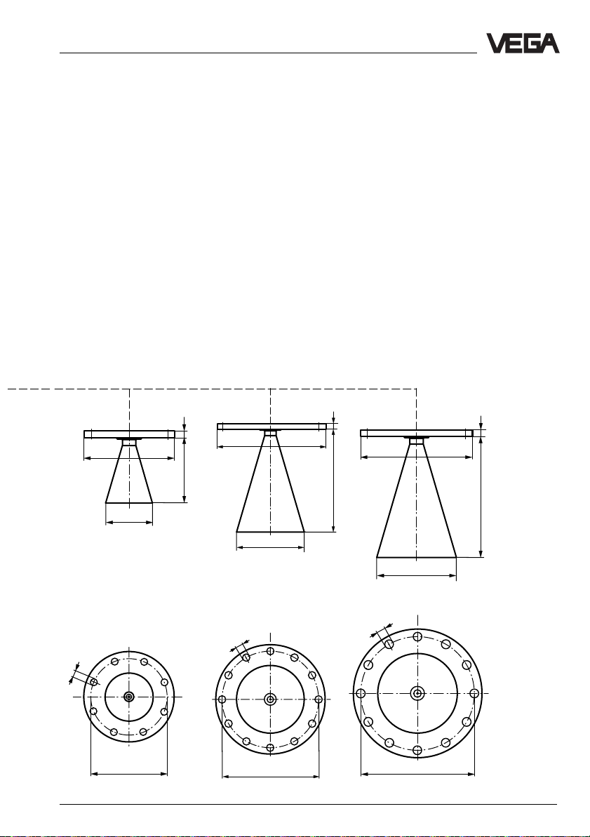
Technical data

ø22

ø285

ø146

ø240

DN 150

205

ø340

ø197

ø22

ø295

DN 200

ø405

296

ø241

ø26

ø355

DN 250

380

VEGAPULS 56 Profibus PA 87

External indicating instrument VEGADIS 50

85 38

ø5

Pg 13,5

Mounting on carrier rail 35 x 7.5 acc. to EN 50 022 or flat screwed

118

108

135

Flange dimensions acc. to ANSI

Technical data

Note:

The cable diameter of the connection cable should be min. 5 mm and max. 9 mm. Otherwise the seal effect of the cable entry

would not be ensured.

D = outer flange diameter

b = flange thickness k = diameter of hole circle d

= seal ledge diameter

f = seal ledge thickness

/16" = approx. 1.6 mm

= diameter of holes

Size Flange Seal ledge Holes

Db k d1No. d

2" 150 psi 152.4 20.7 120.7 91.9 4 19.1 3" 150 psi 190.5 25.5 152.4 127.0 4 19.1 4" 150 psi 228.6 25.5 190.5 157.2 8 19.1 6" 150 psi 279.4 27.0 241.3 215.9 8 22.4

Adjustment module MINICOM

ESC

Tank 1 m (d)

12.345

67,5

32,5

88 VEGAPULS 56 Profibus PA

Adjustment module for insertion into series 50 sensors or into the external indicating instrument VEGADIS 50

Notes

VEGAPULS 56 Profibus PA 89

Notes

90 VEGAPULS 56 Profibus PA

Notes

VEGAPULS 56 Profibus PA 91

VEGA Grieshaber KG Am Hohenstein 113 D-77761 Schiltach Phone (07836) 50-0 Fax (07836) 50-201 E-Mail info@de.vega.com

www.vega.com

ISO 9001

All statements concerning scope of delivery, application, practical use and operating conditions of the sensors and processing systems correspond to the latest information at the time of printing.

Technical data subject to alterations

2.26 386 / July 2001

VEGA PULS56 User Manual

Specifications and Main Features

Frequently Asked Questions

User Manual

Safety information

Note Ex area

1 Product description

1.1 Function

1.2 Application features

1.3 Profibus output signal

1.4 Adjustment

1.5 Antennas

2 Types and versions

2.1 Type surve y

2.2 Type code

2.3 Bus configuration

3 Mounting and installation

3.1 General installation instructions

3.2 Measurement of liquids

3.3 Measurement in standpipe (surge or bypass tube)

3.4 False echoes

3.5 Installation mistakes

4 Electrical connection

4.2 Sensor address

4.3 Connection of the sensor

5 Setup

5.1 Adjustment media

5.2 Adjustment with VV O

6 PA function diagram

7 Diagnosis

7.1 Simulation

7.2 Error codes

8 Technical data

8.1 Data

8.2 Approvals

8.3 Data format of the output signal

8.4 Dimensions