

Page 1

TI-92
GUIDEBOOK
The
Geometry IIè, who are with the Université Joseph Fourier, Grenoble, France.
The
of the
Macintosh is a registered trademark of Apple Computer, Inc.
Cabri Geometry II is a trademark of Université Joseph Fourier.
TI-GRAPH LINK, Calculator-Based Laboratory, CBL, CBL 2, Calculator-Based Ranger,
CBR, Constant Memory, Automatic Power Down, APD, and EOS are trademarks of
Texas Instruments Incorporated.
© 1995–1998, 2001 Texas Instruments Incorporated
Geometry was jointly developed by TI and the authors of Cabri
TI-92
Symbolic Manipulation was jointly developed by TI and the authors
TI-92
program, who are with Soft Warehouse, Inc., Honolulu, HI.
DERIVE
ë
Page 2

Important
Texas Instruments makes no warranty, either expressed or implied,
including but not limited to any implied warranties of
merchantability and fitness for a particular purpose, regarding any
programs or book materials and makes such materials available
solely on an “as-is” basis.
In no event shall Texas Instruments be liable to anyone for special,
collateral, incidental, or consequential damages in connection with or
arising out of the purchase or use of these materials, and the sole and
exclusive liability of Texas Instruments, regardless of the form of
action, shall not exceed the purchase price of this equipment.
Moreover, Texas Instruments shall not be liable for any claim of any
kind whatsoever against the use of these materials by any other party.
US FCC Information
Concerning Radio
Frequency
Interference
This equipment has been tested and found to comply with the limits
for a Class B digital device, pursuant to Part 15 of the FCC rules. These
limits are designed to provide reasonable protection against harmful
interference in a residential installation. This equipment generates,
uses, and can radiate radio frequency energy and, if not installed and
used in accordance with the instructions, may cause harmful
interference with radio communications. However, there is no
guarantee that interference will not occur in a particular installation.
If this equipment does cause harmful interference to radio or
television reception, which can be determined by turning the
equipment off and on, you can try to correct the interference by one
or more of the following measures:
¦
Reorient or relocate the receiving antenna.
¦
Increase the separation between the equipment and receiver.
¦
Connect the equipment into an outlet on a circuit different from
that to which the receiver is connected.
¦
Consult the dealer or an experienced radio/television technician
for help.
Caution:
expressly approved by Texas Instruments may void your authority to
operate the equipment.
Any changes or modifications to this equipment not
ii
Page 3

Table of Contents
This guidebook describes how to use the TI-92. The table of
contents can help you locate “getting started” information as
well as detailed information about the TI-92’s features.
How to Use this Guidebook................................................................... viii
Chapter 1: Getting Started
Chapter 2: Operating the
Chapter 3: Basic Function Graphing
TI-92
Getting the
Performing Computations ........................................................................ 4
Graphing a Function.................................................................................. 7
Constructing Geometric Objects ............................................................. 9
Turning the
Setting the Display Contrast................................................................... 15
The Keyboard ........................................................................................... 16
Home Screen ............................................................................................ 19
Entering Numbers.................................................................................... 21
Entering Expressions and Instructions................................................. 22
Formats of Displayed Results ................................................................ 25
Editing an Expression in the Entry Line............................................... 28
Menus............................................................................................... 30
TI-92
Selecting an Application ......................................................................... 33
Setting Modes ........................................................................................... 35
Using the Catalog to Select a Command............................................... 37
Storing and Recalling Variable Values................................................... 38
Re-using a Previous Entry or the Last Answer..................................... 40
Auto-Pasting an Entry or Answer from the History Area ................... 42
Status Line Indicators in the Display..................................................... 43
Preview of Basic Function Graphing..................................................... 46
Overview of Steps in Graphing Functions............................................ 47
Setting the Graph Mode .......................................................................... 48
Defining Functions for Graphing........................................................... 49
Selecting Functions to Graph................................................................. 51
Setting the Display Style for a Function ............................................... 52
Defining the Viewing Window................................................................ 53
Changing the Graph Format ................................................................... 54
Graphing the Selected Functions........................................................... 55
Displaying Coordinates with the Free-Moving Cursor........................ 56
Tracing a Function................................................................................... 57
Using Zooms to Explore a Graph........................................................... 59
Using Math Tools to Analyze Functions ............................................... 62
Ready to Use................................................................. 2
TI.92
On and Off.................................................................. 14
TI-92
Chapter 4: Tables
Preview of Tables..................................................................................... 68
Overview of Steps in Generating a Table.............................................. 69
Setting Up the Table Parameters ........................................................... 70
Displaying an Automatic Table .............................................................. 72
Building a Manual (Ask) Table............................................................... 75
iii
Page 4

Table of Contents
(Continued)
Chapter 5: Using Split Screens
Chapter 6: Symbolic Manipulation
Chapter 7: Geometry
Preview of Split Screens ......................................................................... 78
Setting and Exiting the Split Screen Mode ........................................... 79
Selecting the Active Application............................................................ 81
Preview of Symbolic Manipulation........................................................ 84
Using Undefined or Defined Variables.................................................. 85
Using Exact, Approximate, and Auto Modes ....................................... 87
Automatic Simplification ........................................................................ 90
Delayed Simplification for Certain Built-In Functions ....................... 92
Substituting Values and Setting Constraints ........................................93
Overview of the Algebra Menu............................................................... 96
Common Algebraic Operations.............................................................. 98
Overview of the Calc Menu................................................................... 101
Common Calculus Operations ............................................................. 102
User-Defined Functions and Symbolic Manipulation ....................... 103
If You Get an Out-of-Memory Error..................................................... 105
Special Constants Used in Symbolic Manipulation........................... 106
Preview of Geometry............................................................................. 108
Learning the Basics................................................................................ 109
Managing File Operations..................................................................... 116
Setting Application Preferences........................................................... 117
Selecting and Moving Objects .............................................................. 120
Deleting Objects from a Construction................................................. 121
Creating Points....................................................................................... 122
Creating Lines, Segments, Rays, and Vectors..................................... 124
Creating Circles and Arcs ..................................................................... 127
Creating Triangles.................................................................................. 129
Creating Polygons.................................................................................. 130
Constructing Perpendicular and Parallel Lines ................................. 132
Constructing Perpendicular and Angle Bisectors.............................. 134
Creating Midpoints ................................................................................ 135
Transferring Measurements.................................................................. 136
Creating a Locus..................................................................................... 138
Redefining Point Definitions ................................................................ 139
Translating Objects................................................................................ 140
Rotating and Dilating Objects .............................................................. 141
Creating Reflections and Inverse Objects........................................... 146
Measuring Objects ................................................................................. 149
Determining Equations and Coordinates............................................ 151
Performing Calculations ....................................................................... 152
Collecting Data....................................................................................... 153
Checking Properties of Objects ........................................................... 154
Putting Objects in Motion..................................................................... 156
Controlling How Objects Are Displayed............................................. 158
Adding Descriptive Information to Objects........................................ 161
Creating Macros ..................................................................................... 164
Geometry Toolbar Menu Items ............................................................ 167
Pointing Indicators and Terms Used in Geometry ............................ 169
Helpful Shortcuts ................................................................................... 170
iv
Page 5

Chapter 8: Data/Matrix Editor
Preview of the Data/Matrix Editor....................................................... 172
Overview of List, Data, and Matrix Variables..................................... 173
Starting a Data/Matrix Editor Session................................................. 175
Entering and Viewing Cell Values........................................................ 177
Inserting and Deleting a Row, Column, or Cell.................................. 180
Defining a Column Header with an Expression................................. 182
Using Shift and CumSum Functions in a Column Header................ 184
Sorting Columns..................................................................................... 185
Saving a Copy of a List, Data, or Matrix Variable .............................. 186
Chapter 9: Statistics and Data Plots
Chapter 10: Additional Home Screen Topics
Chapter 11: Parametric Graphing
Preview of Statistics and Data Plots.................................................... 188
Overview of Steps in Statistical Analysis............................................ 192
Performing a Statistical Calculation.................................................... 193
Statistical Calculation Types................................................................ 195
Statistical Variables ............................................................................... 197
Defining a Statistical Plot...................................................................... 198
Statistical Plot Types............................................................................. 200
Using the Y= Editor with Stat Plots..................................................... 202
Graphing and Tracing a Defined Stat Plot.......................................... 203
Using Frequencies and Categories ...................................................... 204
If You Have a CBL 2/CBL or CBR........................................................206
Saving the Home Screen Entries as a Text Editor Script ................. 210
Cutting, Copying, and Pasting Information ........................................211
Creating and Evaluating User-Defined Functions ............................. 213
Using Folders to Store Independent Sets of Variables ..................... 216
If an Entry or Answer Is “Too Big” ......................................................219
Preview of Parametric Graphing.......................................................... 222
Overview of Steps in Graphing Parametric Equations...................... 223
Differences in Parametric and Function Graphing............................ 224
Chapter 12: Polar Graphing
Chapter 13: Sequence Graphing
Preview of Polar Graphing.................................................................... 228
Overview of Steps in Graphing Polar Equations................................ 229
Differences in Polar and Function Graphing...................................... 230
Preview of Sequence Graphing ............................................................ 234
Overview of Steps in Graphing Sequences ......................................... 235
Differences in Sequence and Function Graphing .............................. 236
Setting Axes for Time, Web, or Custom Plots.................................... 240
Using Web Plots ..................................................................................... 241
Using Custom Plots ............................................................................... 244
Using a Sequence to Generate a Table................................................ 245
Comparison of
TI-92
and
Sequence Functions.......................... 246
TI-82
v
Page 6

Table of Contents
(Continued)
Chapter 14: 3D Graphing
Chapter 15: Additional Graphing Topics
Chapter 16: Text Editor
Preview of 3D Graphing........................................................................ 248
Overview of Steps in Graphing 3D Equations .................................... 249
Differences in 3D and Function Graphing.......................................... 250
Moving the Cursor in 3D ....................................................................... 253
Rotating and/or Elevating the Viewing Angle..................................... 255
Changing the Axes and Style Formats ................................................ 257
Preview of Additional Graphing Topics.............................................. 260
Collecting Data Points from a Graph .................................................. 261
Graphing a Function Defined on the Home Screen........................... 262
Graphing a Piecewise Defined Function............................................. 264
Graphing a Family of Curves................................................................ 266
Using the Two-Graph Mode.................................................................. 267
Drawing a Function or Inverse on a Graph ........................................ 270
Drawing a Line, Circle, or Text Label on a Graph ............................. 271
Saving and Opening a Picture of a Graph........................................... 275
Animating a Series of Graph Pictures ................................................. 277
Saving and Opening a Graph Database ............................................... 278
Preview of Text Operations.................................................................. 280
Starting a Text Editor Session.............................................................. 281
Entering and Editing Text..................................................................... 283
Entering Special Characters ..................................................................286
Entering and Executing a Command Script....................................... 288
Creating a Lab Report............................................................................ 290
Chapter 17: Programming
vi
Preview of Programming ...................................................................... 294
Running an Existing Program .............................................................. 296
Starting a Program Editor Session....................................................... 298
Overview of Entering a Program ......................................................... 300
Overview of Entering a Function......................................................... 303
Calling One Program from Another..................................................... 305
Using Variables in a Program ............................................................... 306
String Operations ................................................................................... 308
Conditional Tests ................................................................................... 310
Using If, Lbl, and Goto to Control Program Flow.............................. 311
Using Loops to Repeat a Group of Commands.................................. 313
............................................................................. 316
Configuring the
Getting Input from the User and Displaying Output .........................317
Creating a Table or Graph..................................................................... 319
Drawing on the Graph Screen .............................................................. 321
Accessing Another
Debugging Programs and Handling Errors......................................... 324
Example: Using Alternative Approaches ............................................ 325
TI-92
a CBL 2/CBL, or a CBR..............................323
TI-92,
Page 7

Chapter 18: Memory and Variable Management
Preview of Memory and Variable Management ................................. 328
Checking and Resetting Memory ......................................................... 330
Displaying the
Manipulating Variables and Folders with
Pasting a Variable Name to an Application ........................................ 335
Transmitting Variables between Two
Transmitting Variables under Program Control................................. 339
VAR-LINK
Screen........................................................... 331
VAR-LINK
s ...................................... 336
TI-92
.......................... 333
Chapter 19: Applications
Appendix A: TI-92 Functions and Instructions
App. 1: Analyzing the Pole-Corner Problem ....................................... 342
App. 2: Deriving the Quadratic Formula ............................................. 344
App. 3: Exploring a Matrix.................................................................... 346
App. 4: Exploring cos(x) = sin(x) ........................................................ 347
App. 5: Finding Minimum Surface Area of a Parallelepiped ............ 348
App. 6: Running a Tutorial Script Using the Text Editor.................. 350
App. 7: Decomposing a Rational Function ......................................... 352
App. 8: Studying Statistics: Filtering Data by Categories ................. 354
App. 9: CBL 2/CBL Program for the TI
App. 10: Studying the Flight of a Hit Baseball.................................... 358
App. 11: Visualizing Complex Zeros of a Cubic Polynomial .............. 360
App. 12: Exploring Euclidean Geometry............................................. 362
App. 13: Creating a Trisection Macro in Geometry ........................... 364
App. 14: Solving a Standard Annuity Problem ................................... 367
App. 15: Computing the Time-Value-of-Money .................................. 368
App. 16: Finding Rational, Real, and Complex Factors .................... 369
App. 17: A Simple Function for Finding Eigenvalues........................ 370
App. 18: Simulation of Sampling without Replacement.................... 371
Quick-Find Locator................................................................................ 374
Alphabetical Listing of Operations ...................................................... 377
92..........................................357
-
Appendix B: Reference Information
Appendix C: Service and Warranty Information
Index
TI-92 Error Messages ............................................................................ 472
TI-92 Modes............................................................................................ 479
TI-92 Character Codes .......................................................................... 483
TI-92 Key Map ........................................................................................ 484
Complex Numbers ................................................................................. 488
Accuracy Information............................................................................ 490
System Variables and Reserved Names .............................................. 491
EOSé (Equation Operating System) Hierarchy................................. 492
Battery Information ............................................................................... 496
In Case of Difficulty............................................................................... 498
Support and Service Information......................................................... 499
Warranty Information............................................................................ 500
General Index ......................................................................................... 503
Geometry Index...................................................................................... 516
vii
Page 8

p
How to Use this Guidebook
The last thing most people want to do is read a book of
instructions before using a new product. With the
can perform a variety of calculations without opening the
guidebook. However, by reading at least parts of the book and
skimming through the rest, you can learn about capabilities
that let you use the
more effectively.
TI-92
TI-92
, you
How the Guidebook Is Organized
Which Chapters Should You Read?
The
screen, Y= Editor, Graph screen, Geometry, etc.) that are explained
in this guidebook. Generally, the guidebook is divided into three
major parts.
¦
¦
¦
Particularly when you first get started, you may not need to use all of
the
that apply to you. It’s a little like the dictionary. If you’re looking for
xylophone, skip A through W.
If you want to: Go to:
Get an overview
of the
capabilities
has a wide variety of features and applications (Home
TI-92
Chapters 1 – 9 cover topics that are often used by people who are
just getting started with the
Chapters 10 – 19 cover additional topics that may not be used
right away (depending on your situation).
The appendices provide useful reference information, as well as
service and warranty information.
’s capabilities. Therefore, you only need to read the chapters
TI-92
Chapter 1
TI-92
and its
to get you started performing calculations,
graphing functions, constructing geometric
objects, etc.
Chapter 2
about operating the
chapter primarily covers the Home screen,
much of the information applies to any
application.
.
TI-92
— Contains step-by-step examples
— Gives general information
. Although this
TI-92
Learn about a
articular
application or
topic
Although you don’t need to read every chapter, skim through the
entire guidebook and stop at anything that interests you. You may
find a feature that could be very useful, but you might not know it
exists if you don’t look around.
viii
The applicable chapter
learn how to graph a function, go to
Chapter 3: Basic Function Graphing.
Most chapters start with a step-by-step
“preview” example that illustrates one or
more of the topics covered in that chapter.
— For example, to
Page 9

How Do I Look Up Information?
Because the book is big, it’s important that you know how to look
things up quickly. Use the:
¦
Table of contents
¦
Index
¦
Appendix A (for detailed information about a particular
function or instruction)
TI-92
Notes about Appendix A
Long after you learn to use the
a valuable reference.
¦
You can access most of the
selecting them from menus. Use Appendix A for details about the
arguments and syntax used for each function and instruction.
− You can also use the Help information that is displayed at the
bottom of the
¦
At the beginning of Appendix A, the available functions and
instructions are grouped into categories. This can help you locate
a function or instruction if you don’t know its name.
− Also refer to Chapter 17, which categorizes program
commands.
CATALOG
, Appendix A can continue to be
TI-92
’s functions and instructions by
TI-92
menu, as described in Chapter 2.
ix
Page 10
Chapter 1: Getting Started
Getting the TI-92 Ready to Use ................................................................ 2
Performing Computations ........................................................................ 4
Graphing a Function.................................................................................. 7
Constructing Geometric Objects ............................................................. 9
1
This chapter helps you to get started using the
chapter takes you through several examples to introduce you to
some of the principle operating and graphing functions of the
.
TI-92
After setting up your
read Chapter 2: Operating the
advance to the detailed information provided in the remaining
chapters in this guidebook.
and completing these examples, please
TI-92
. You then will be prepared to
TI-92
quickly. This
TI-92
Chapter 1: Getting Started 1
Page 11
Getting the TI.92 Ready to Use
2
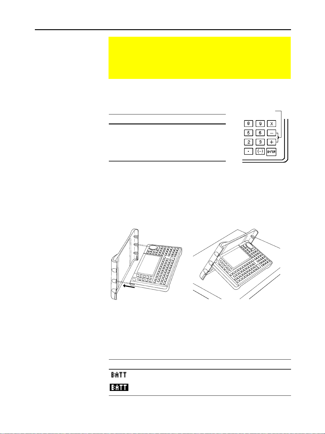
The TI-92 comes with four AA batteries. This section
describes how to install these batteries, turn the unit on for the
first time, set the display contrast, and view the Home screen.
Installing the AA Batteries
Important: When replacing
batteries in the future,
ensure that the
turned off by pressing
®.
TI-92
is
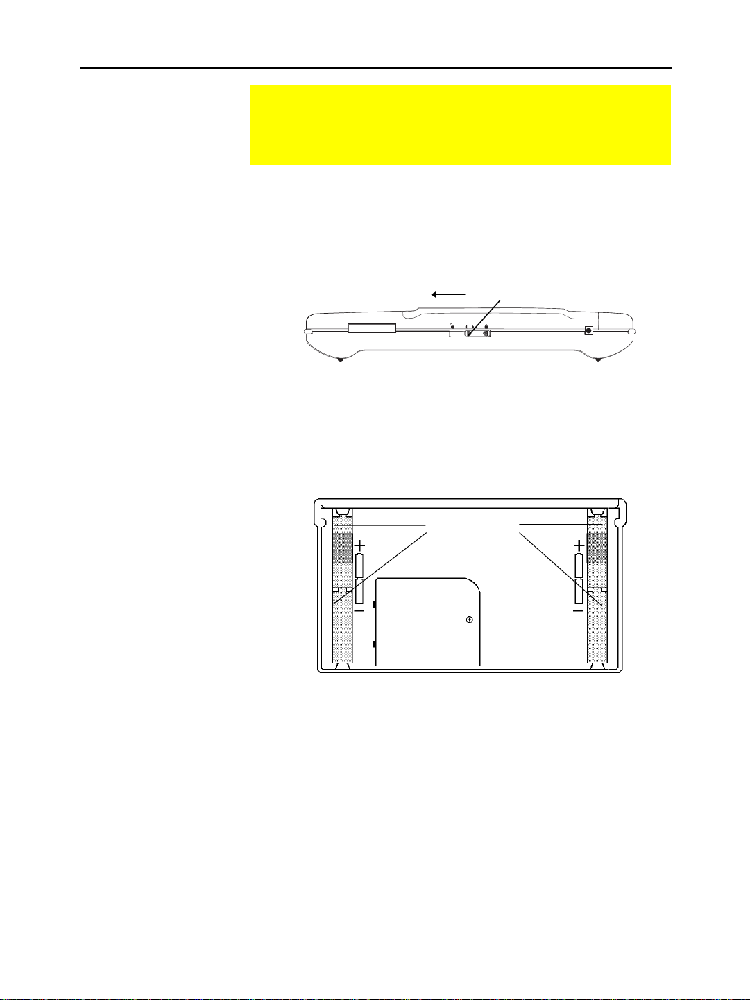
To install the four AA alkaline batteries:
1. Holding the
unit upright, slide the latch on the top of the
TI-92
unit to the right unlocked position; slide the rear cover down
about one-eighth inch and remove it from the main unit.
2. Place the
Slide to open.
I/O
face down on a soft cloth to prevent scratching the
TI-92
top
display face.
3. Install the four AA batteries. Be sure to position the batteries
according to the diagram inside the unit. The positive (+) terminal
of each battery should point toward the top of the unit.
AA batteries
back
4. Replace the rear cover and slide the latch on the top of the unit to
Turning the Unit On and Adjusting the Display Contrast
To turn the unit on and adjust the display after installing the
batteries:
1. Press ´ to turn the
2. To adjust the display to your satisfaction, hold down ¥
2 Chapter 1: Getting Started
the left locked position to lock the cover back in place.
on.
TI-92
The Home screen is displayed; however, the display contrast may
be too dark or too dim to see anything. (When you want to turn
the
off, press 2 ®.)
TI-92
(diamond symbol inside a green border) and momentarily press
| (minus key) to lighten the display. Hold down ¥ and
momentarily press « (plus key) to darken the display.
Page 12
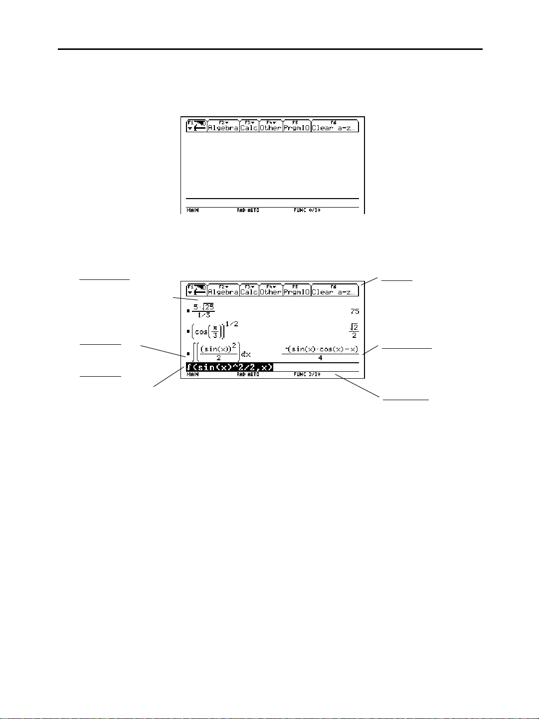
About the Home Screen
When you first turn on your
, a blank Home screen is displayed.
TI-92
The Home screen lets you execute instructions, evaluate
expressions, and view results.
The following example contains previously entered data and
describes the main parts of the Home screen. Entry/answer pairs in
the history area are displayed in “pretty print.”
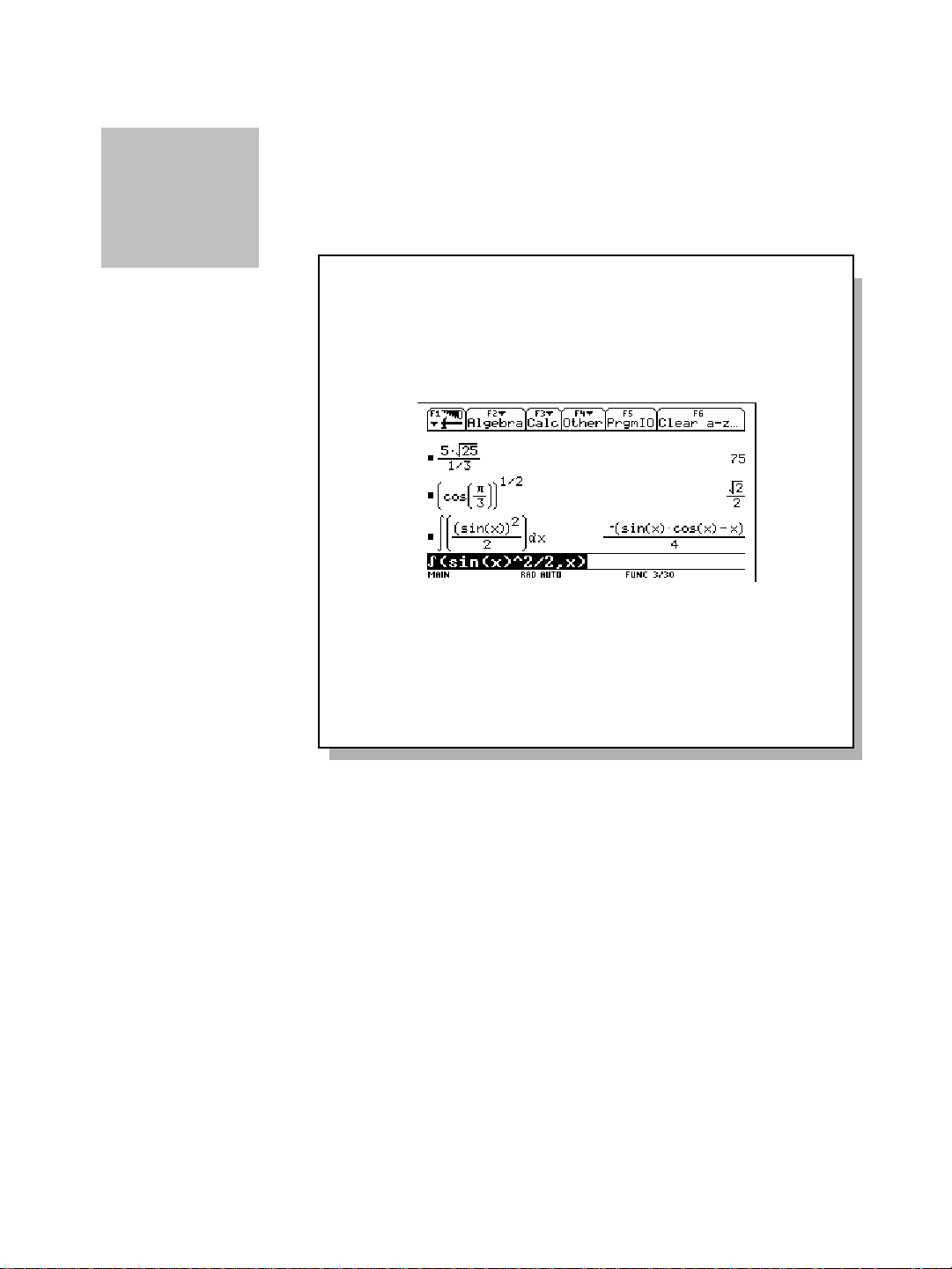
History Area
Lists entry/answer pairs
you have entered. Pairs
scroll up the screen as
you make new entries.
Last Entry
Your last entry.
Entry Line
Where you enter
expressions or
instructions.
Toolbar
Lets you display menus for
selecting operations
applicable to the Home
screen. To display a toolbar
menu, press ƒ, „, etc.
Last Answer
Result of your last entry.
Note that results are not
displayed on the entry line.
Status Line
Shows the current state
of the calculator.
Chapter 1: Getting Started 3
Page 13
Performing Computations
This section provides several examples for you to perform that demonstrate some of the
computational features of the TI-92. The history area in each screen was cleared by
pressing ƒ and selecting 8:Clear Home, before performing each example, to illustrate
only the results of the example’s keystrokes.
Steps Keystrokes Display
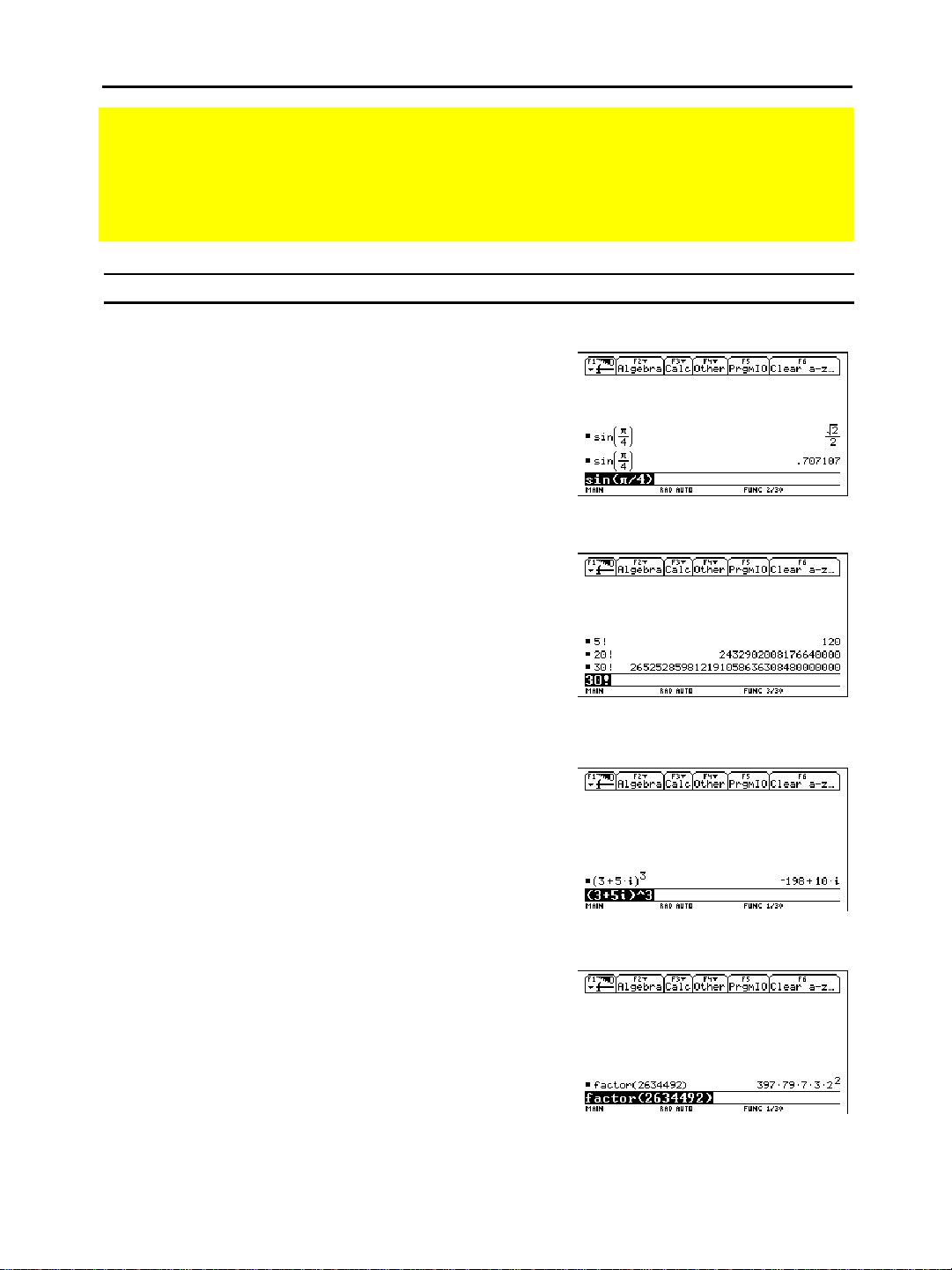
Showing Computations
1. Compute
sin(p/4)
and display the
result in symbolic and numeric
format.
To clear the history area of previous
calculations, press
Home.
and select
ƒ
8:Clear
Finding the Factorial of Numbers
1. Compute the factorial of several
numbers to see how the TI-92
handles very large integers.
To get the factorial operator (!), press
2 I, select
select
1:!
.
7:Probability
, and then
Expanding Complex Numbers
3
1. Compute
to see how the TI-92
(3+5i)
handles computations involving
complex numbers.
W2T
e4d¸¥
¸
5 2I71
¸
202I71
¸
302I71
¸
c 3 « 5 2)
dZ3¸
Finding Prime Factors
1. Compute the factors of the rational
number
You can enter “factor” on the entry line by
typing
pressing
Optional
2. (
2634492
FACTOR
„
.
on the keyboard, or by
and selecting
2:factor(
.
) Enter other numbers on
your own.
4 Chapter 1: Getting Started
FACTORc
2634492d
¸
Page 14
Steps Keystrokes Display
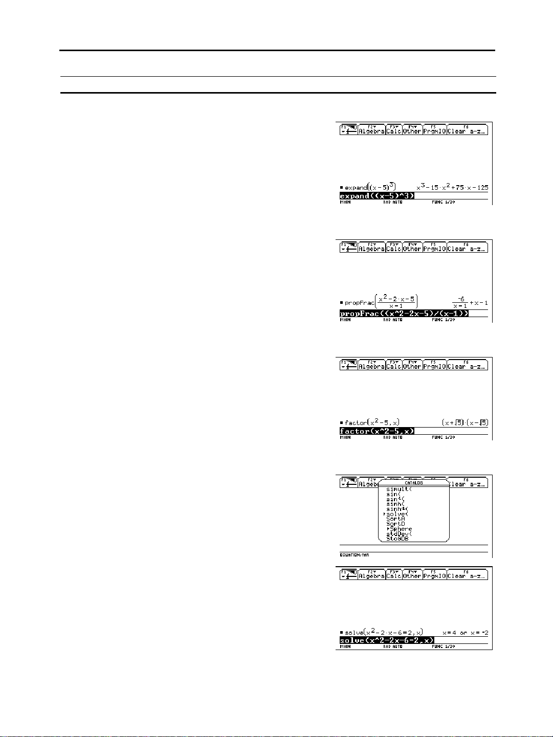
Expanding Expressions
3
1. Expand the expression
You can enter “expand” on the entry line by
typing
EXPAND
pressing
on the keyboard, or by
and selecting
„
3:expand(
(xì5)
.
.
EXPANDc
cX|5d
Z3d
¸
2. (Optional) Enter other expressions
on your own.
Reducing Expressions
2
1. Reduce the expression
(x
ì2xì
5)/(xì1)
to its simplest form.
You can enter “propFrac” on the entry line
by typing
by pressing
PROPFRAC
„
on the keyboard, or
and selecting
7:propFrac(.
PROPFRACc
cXZ2|2X
|5de
cX|1dd
¸
Factoring Polynomials
2
ì
1. Factor the polynomial
respect to
You can enter “factor” on the entry line by
typing
pressing
x
FACTOR
and selecting
„
.
on the keyboard or by
5)
(x
2:factor(
with
.
FACTORc
XZ2|5
bXd
¸
Solving Equations
2
1. Solve the equation
respect to
You can enter “solve(” on the entry line by
selecting
typing
pressing
The status line area shows the required
syntax for the marked item in the Catalog
menu.
x
“solve(”
SOLVE(
and selecting
„
.
on the keyboard, or by
ì2xì
x
from the Catalog menu, by
6=2
1:solve(
with
.
2½S
(press D until
the ú mark
points to
¸
solve(
X Z 2 | 2X|6
Á2bXd
¸
)
Chapter 1: Getting Started 5
Page 15
Performing Computations
Steps Keystrokes Display
(Continued)
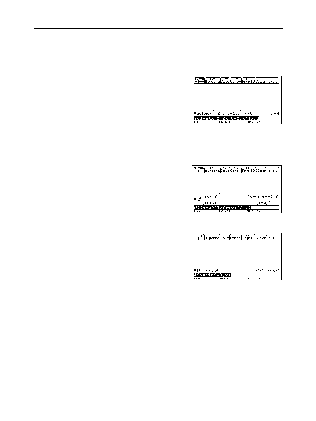
Solving Equations with a Domain
Constraint
1. Solve the equation
respect to
where x is greater than
x
zero.
Pressing
operator (domain constraint).
produces the “with” (I)
K
2
x
ì2xì
6=2
with
2½S
(press D until
the ú mark
points to
¸
solve(
X Z 2 | 2X|6
Á2
bXd2KX
2Ã0
¸
)
2
Finding the Derivative of Functions
1. Find the derivative of
(xìy)3/(x+y)
2
with respect to x.
This example illustrates using the calculus
differentiation function and how the function
is displayed in “pretty print” in the history
area.
2=cX|Y
dZ3ecX«
YdZ2bXd
¸
Finding the Integral of Functions
1. Find the integral of
respect to
This example illustrates using the calculus
integration function.
.
x
xùsin(x)
with
2<XpW
XdbXd
¸
6 Chapter 1: Getting Started
Page 16
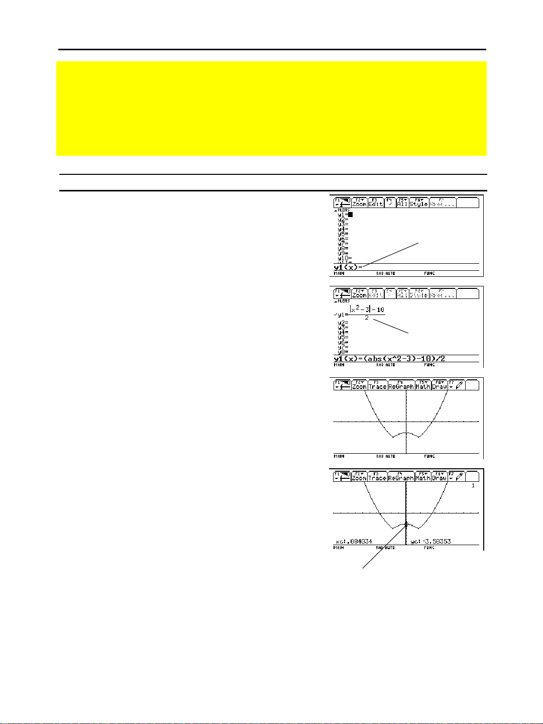
Graphing a Function
The example in this section demonstrates some of the graphing capabilities of the
It illustrates how to graph a function using the Y= Editor. You will learn how to enter a
function, produce a graph of the function, trace a curve, find a minimum point, and
transfer the minimum coordinates to the Home screen.
2
Explore the graphing capabilities of the
by graphing the function
TI-92
Steps Keystrokes Display
1. Display the Y= Editor.
2. Enter the function
(abs(x
2
ì3)ì
10)/2
¥#
.
c ABScXZ2
|3d|10d
e2¸
y=(|x
ì3|ì
“pretty print”
display of the
function in the
entry line
TI-92
.
10)/2
entry line
.
3. Display the graph of the function.
Select
6:ZoomStd
moving the cursor to
pressing
¸
by pressing 6 or by
6:ZoomStd
.
and
4. Turn on Trace.
The tracing cursor, and the x and y
coordinates are displayed.
„ 6
…
tracing
cursor
Chapter 1: Getting Started 7
Page 17
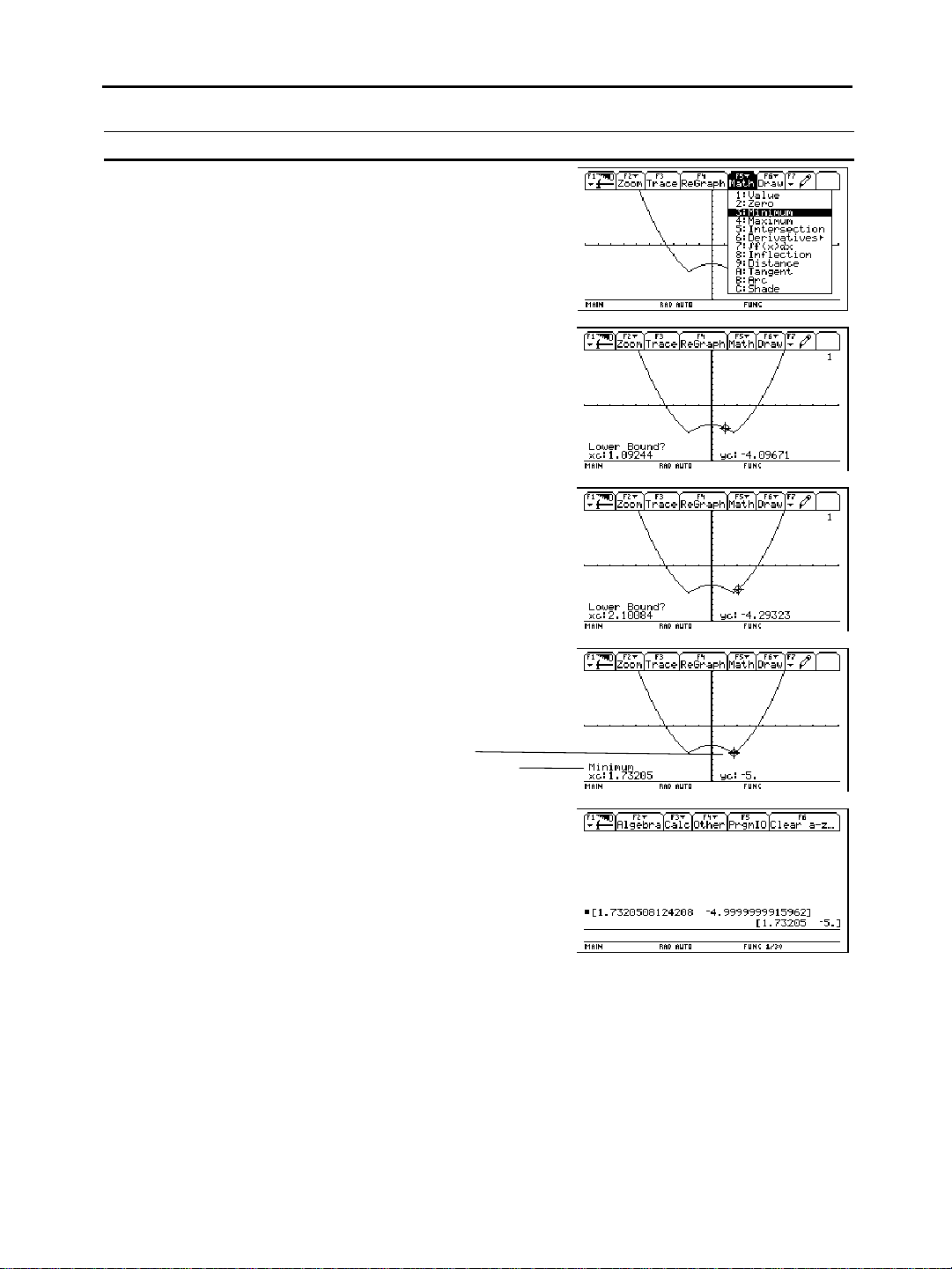
Graphing a Function
Steps Keystrokes Display
(Continued)
5. Open the
3:Minimum
menu and select
MATH
.
6. Set the lower bound.
Press B (right cursor) to move the tracing
cursor until the lower bound for x is just to
the left of the minimum node before
pressing
the second time.
¸
7. Set the upper bound.
Press B (right cursor) to move the tracing
cursor until the upper bound for x is just to
the right of the minimum node.
8. Find the minimum point on the graph
between the lower and upper bounds.
‡DD
¸
B
B
...
¸
B
B
...
¸
9. Transfer the result to the Home
screen, and then display the Home
screen.
8 Chapter 1: Getting Started
minimum point
minimum coordinates
¥ H
¥"
Page 18
Constructing Geometric Objects
This section provides a multi-part example about constructing
geometric objects using the Geometry application of the
You will learn how to construct a triangle and measure its
area, construct perpendicular bisectors to two of the sides,
and construct a circle centered at the intersection of the two
bisectors that will circumscribe the triangle.
TI-92
.
Getting Started in Geometry
Note: Each of the following
example modules require
that you complete the
previous module.
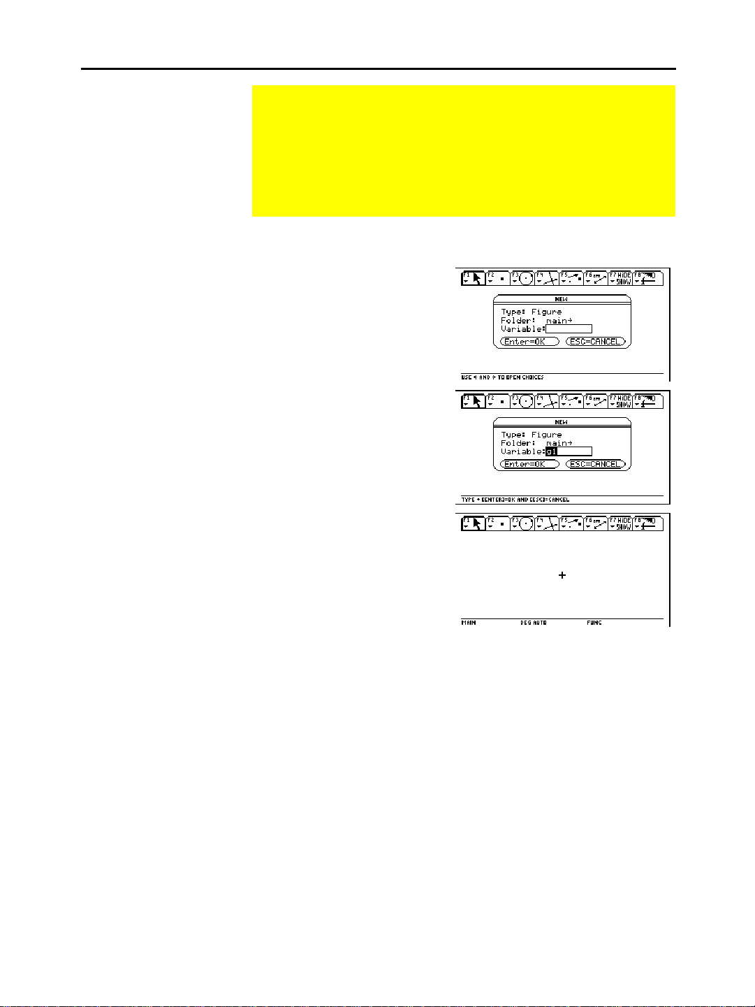
To start a Geometry session, you first have to give it a name.
83
1. Press O
the
dialog box.
New
to display
2. Press DG1 as the name
for the new construction,
and press ¸.
3. Press ¸ to display the
Geometry drawing
window.
Chapter 1: Getting Started 9
Page 19
Constructing Geometric Objects
(Continued)
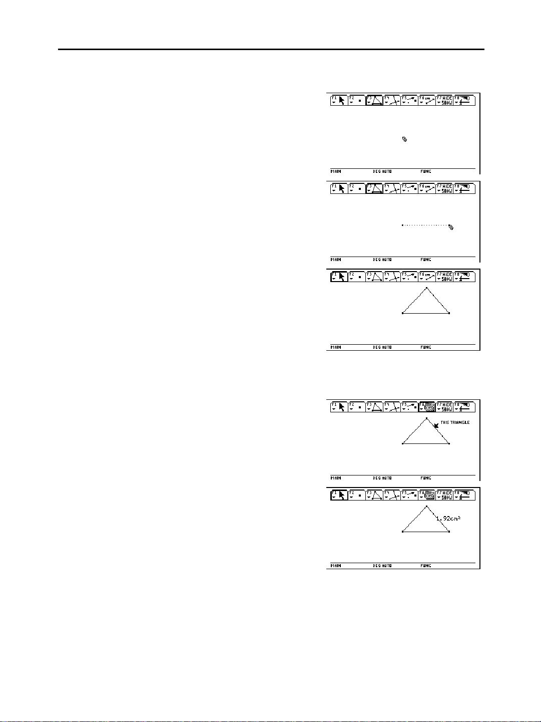
Creating a Triangle
To create a triangle:
1. Press … and select
3:Triangle
.
2. Move the cursor (#) to the
desired location, and press
¸ to define the first
point.
3. Move the cursor to another
location, and press ¸
to define the second point.
4. Move the cursor to the
third location, and press
¸ again to complete
the triangle.
Measuring the Area of the Triangle
Note: Default
measurements are in
centimeters. See “Setting
Application Preferences” in
Chapter 7 to change to
other unit measurements.
To measure the area of the triangle that you constructed in the
previous example:
1. Press ˆ and select
2:Area.
2. Move the cursor, if
necessary, until
TRIANGLE”
“THIS
is displayed.
3. Press ¸ to display the
result.
10 Chapter 1: Getting Started
Page 20
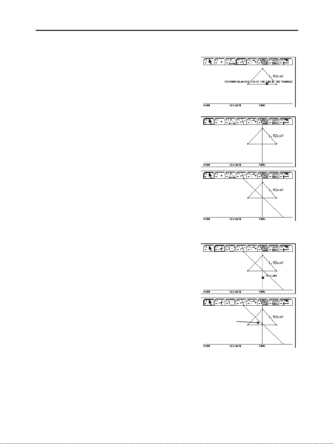
Constructing the Perpendicular Bisectors
To construct the perpendicular bisector to two sides of the triangle:
1. Press † and select
4:Perpendicular Bisector
2. Move the cursor close to
the triangle until a
message is displayed that
indicates a side of the
triangle.
3. Press ¸ to construct
the first bisector.
4. Move the cursor to one of
the other two sides until
the message is displayed
(same as step 2), and press
¸ to construct the
second bisector.
.
Finding the Intersection Point of Two Lines
To find the intersection point of the two bisectors:
1. Press „ and select
3:Intersection Point
2. Select the first line, and
then press ¸.
3. Select the second line, and
then press ¸ to create
the intersection point.
.
Chapter 1: Getting Started 11
Page 21
Constructing Geometric Objects
(Continued)
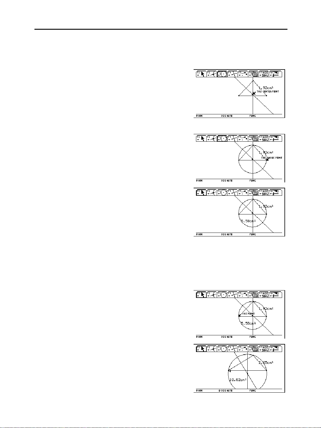
Creating a Circle
Hint: See “Measuring the
Area of the Triangle” on the
previous page.
To create a circle whose centerpoint is at the intersection of the two
bisectors and whose radius is attached to one of the triangle’s vertex
points:
1. Press … and select
1:Circle
.
2. Move the cursor to the
intersection point of the
two perpendicular
bisectors, and press ¸
to define the centerpoint
of the circle.
3. Move the cursor away
from the centerpoint to
expand the circle until the
cursor is near one of the
vertices of the triangle and
“THIS RADIUS POINT”
appears.
4. Press ¸ to construct
the circle.
5. Measure the area of the
circle.
Effects of Modifying the Triangle
This example illustrates the interactive features of the
grab one vertex of the triangle to modify the triangle’s shape. The
size of the circle, as well as the areas of the triangle and circle, will
change accordingly.
To observe the interactive features of the
1. Press ƒ and select
Note: The circle stays
attached to the triangle, and
the areas of the triangle and
circle change.
12 Chapter 1: Getting Started
2. Press and hold ‚
1:Pointer.
Move the cursor
to one of the intersecting
points of the circle and
triangle until
“THIS POINT”
appears, and then press
¸.
(dragging hand) with your
left thumb while pressing
the cursor with your right
thumb to drag the selected
point to its new location.
TI-92
. You will
TI-92
:
Page 22

Chapter 2:
Operating the TI.92
2
Turning the
Setting the Display Contrast................................................................... 15
The Keyboard ........................................................................................... 16
Home Screen ............................................................................................ 19
Entering Numbers.................................................................................... 21
Entering Expressions and Instructions................................................. 22
Formats of Displayed Results ................................................................ 25
Editing an Expression in the Entry Line............................................... 28
Menus............................................................................................... 30
TI-92
Selecting an Application ......................................................................... 33
Setting Modes ........................................................................................... 35
Using the Catalog to Select a Command............................................... 37
Storing and Recalling Variable Values................................................... 38
Reusing a Previous Entry or the Last Answer...................................... 40
Auto-Pasting an Entry or Answer from the History Area ................... 42
Status Line Indicators in the Display..................................................... 43
This chapter gives a general overview of the
its basic operations. By becoming familiar with the information in
this chapter, you can use the
effectively.
On and Off.................................................................. 14
TI-92
and describes
TI-92
to solve problems more
TI-92
The Home screen is the most commonly used application on the
. You can use the Home screen to perform a wide variety of
TI-92
mathematical operations.
Chapter 2: Operating the TI.92 13
Page 23

p
p
Turning the
TI.92
On and Off
Turning the
TI.92
On
Turning the
TI.92
Off
Note:
function of the ´ key.
is the second
®
You can turn the TI-92 on and off manually by using the
and 2 ® (or ¥ ® ) keys. To prolong battery life, the
APDé (Automatic Power Down) feature lets the TI-92 turn
itself off automatically.
Press ´.
¦
If you turned the unit off by pressing 2 ®, the
Home screen as it was when you last used it.
¦
If you turned the unit off by pressing ¥ ® or if the unit turned
itself off through APD, the
You can use either of the following keys to turn off the
Press: Description
2 ®
(press 2
and then
ress ®)
Settings and memory contents are retained by the
Constant Memoryé feature. However:
¦
You cannot use 2 ® if an error message is
displayed.
¦
When you turn the
displays the Home screen (regardless of the last
application you used).
will be exactly as you left it.
TI-92
on again, it always
TI-92
TI-92
TI-92
shows the
´
.
APD (Automatic Power Down)
Batteries
¥ ®
(press ¥
and then
ress ®)
After several minutes without any activity, the
automatically. This feature is called APD.
When you press ´, the
¦
The display, cursor, and any error conditions are exactly as you
left them.
¦
All settings and memory contents are retained.
APD does not occur if a calculation or program is in progress, unless
the program is paused.
The
battery. To replace the batteries without losing any information
stored in memory, follow the directions in Appendix C.
uses four AA alkaline batteries and a back-up lithium
TI-92
Similar to 2 ® except:
¦
You can use ¥ ® if an error message is
displayed.
¦
When you turn the
exactly as you left it.
will be exactly as you left it.
TI-92
on again, it will be
TI-92
TI-92
turns itself off
14 Chapter 2: Operating the TI.92
Page 24
Setting the Display Contrast
The brightness and contrast of the display depend on room
lighting, battery freshness, viewing angle, and the adjustment
of the display contrast. The contrast setting is retained in
memory when the
is turned off.
TI-92
Adjusting the Display Contrast
Using the Snap-on Cover as a Stand
Note: Slide the tabs at the
top-sides of the
the slots in the cover.
TI-92
into
You can adjust the display contrast to suit your viewing angle and
lighting conditions.
Contrast keys
To: Press and hold both:
Increase (darken)
¥ and «
the contrast
Decrease (lighten)
¥ and |
the contrast
If you press and hold ¥ « or ¥ | too long, the display may go
completely black or blank. To make finer adjustments, hold ¥ and
then tap « or |.
on a desk or table top, you can use the snap-on
When using the
TI-92
cover to prop up the unit at one of three angles. This may make it
easier to view the display under various lighting conditions.
When to Replace Batteries
Tip: The display may be
very dark after you change
batteries. Use ¥ | to
lighten the display.
As the batteries get low, the display begins to dim (especially during
calculations) and you must increase the contrast. If you have to
increase the contrast frequently, replace the four AA batteries.
The status line along the bottom of the display also gives battery
information.
Indicator in status line Description
Batteries are low.
Replace batteries as soon as possible.
Chapter 2: Operating the TI.92 15
Page 25
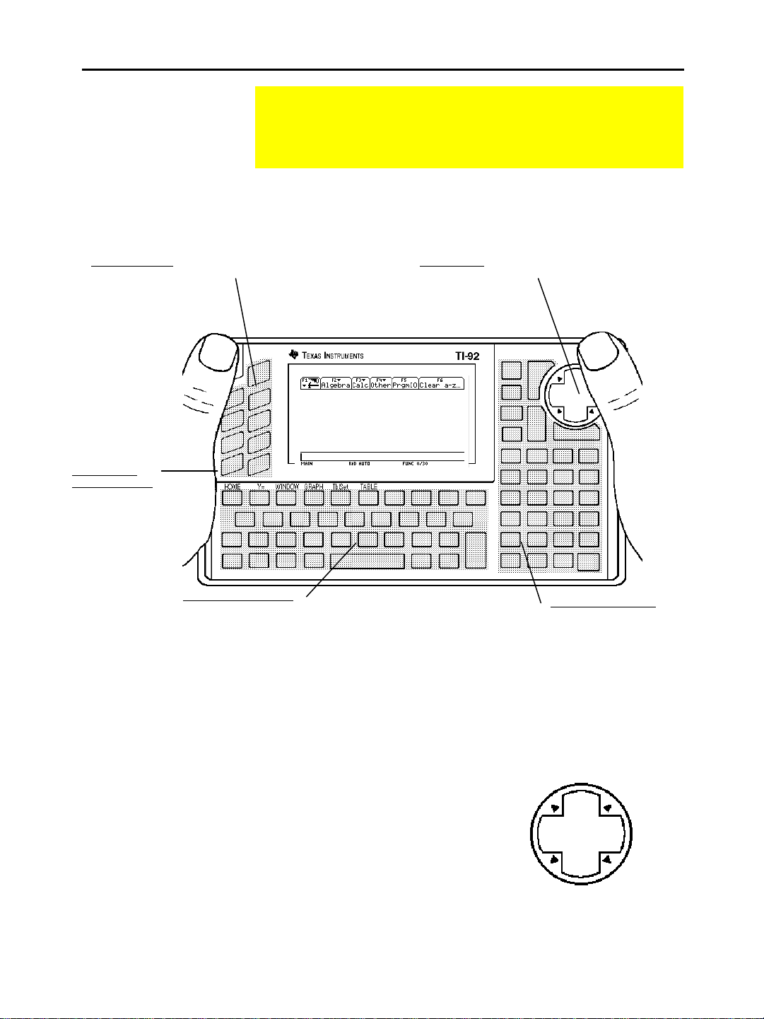
The Keyboard
j
Keyboard Areas
Function Keys
Access the toolbar menus
displayed across the top
of the screen.
Application
Shortcut Keys
Used with the
¥
key to let
you select
commonly used
applications.
With the
’s easy-to-hold shape and keyboard layout, you
TI-92
can quickly access any area of the keyboard even when you
are holding the unit with two hands.
The keyboard is divided into several areas of related keys.
Cursor Pad
Moves the display
cursor in up to 8
directions, depending
on the application.
Cursor Pad
QWERTY Keyboard
Enters text characters
ust as you would on a
typewriter.
To move the cursor, press the applicable edge of the cursor pad. This
Calculator Keypad
Performs a variety of
math and scientific
operations.
guidebook uses key symbols such as A and B to indicate which
side of the cursor pad to press.
C
For example, press B to move the
cursor to the right.
The diagonal directions
Note:
A
B
(H, etc.) are used only for
geometry and graphing
applications.
D
16 Chapter 2: Operating the TI.92
Page 26

Important Keys You Should Know About
The area around the cursor pad contains several keys that are
important for using the
Key Description
TI-92
effectively.
O Displays a menu that lists all the applications available
on the
and lets you select the one you want. Refer
TI-92
to page 33.
N Cancels any menu or dialog box.
¸ Evaluates an expression, executes an instruction,
selects a menu item, etc.
Because this is commonly used in a variety of
operations, the
has three ¸ keys placed at
TI-92
convenient locations.
2
is a modifier
key, which is
described below.
Modifier Keys
3 Displays a list of the
’s current mode settings,
TI-92
which determine how numbers and graphs are
interpreted, calculated, and displayed. You can change
the settings as needed. Refer to “Setting Modes” on
page 35.
M Clears (erases) the entry line. Also used to delete an
entry/answer pair in the history area.
Most keys can perform two or more functions, depending on
whether you first press a modifier key.
Modifier Description
2
(Second)
Accesses the second function of the next key you
press. On the keyboard, second functions are printed in
the same color as the 2 key.
The
has two 2 keys conveniently placed at
TI-92
opposite corners of the keyboard.
¥
(Diamond)
Activates “shortcut” keys that select applications and
certain menu items directly from the keyboard. On the
keyboard, application shortcuts are printed in the same
color as the ¥ key. Refer to page 34.
¤
(Shift)
‚
(Hand)
Types an uppercase character for the next letter key
you press. ¤ is also used with B and A to highlight
characters in the entry line for editing purposes.
Used with the cursor pad to manipulate geometric
objects. ‚ is also used for drawing on a graph.
Chapter 2: Operating the TI.92 17
Page 27

The Keyboard
(Continued)
2nd Functions
Note: On the keyboard,
second functions are printed
in the same color as the
2
key.
Entering Uppercase
Letters with Shift
(¤) or Caps Lock
On the
’s keyboard, a key’s second function is printed above the
TI-92
key. For example:
SINê -------------------
SIN
---------------- Primary function
Second function
To access a second function, press the 2 key and then press the
key for that second function.
In this guidebook:
Primary functions are shown in a box, such as W.
¦
Second functions are shown in brackets, such as 2
¦
When you press 2,
the display. This indicates that the
is shown in the status line at the bottom of
2ND
will use the second function,
TI-92
Q
.
if any, of the next key you press. If you press 2 by accident, press
2
again (or press N) to cancel its effect.
Normally, the
QWERTY
keyboard types lowercase letters. To type
uppercase letters, use Shift and Caps Lock just as on a typewriter.
To: Do this:
Type a single
uppercase letter
Press ¤ and then the letter key.
To type multiple uppercase letters,
¦
hold ¤ or use Caps Lock.
If You Need to Enter Special Characters
When Caps Lock is on, ¤ has no effect.
¦
Toggle Caps Lock
Press 2
¢
.
on or off
You can also use the
QWERTY
keyboard to enter a variety of special
characters. For more information, refer to “Entering Special
Characters” in Chapter 16.
18 Chapter 2: Operating the TI.92
Page 28
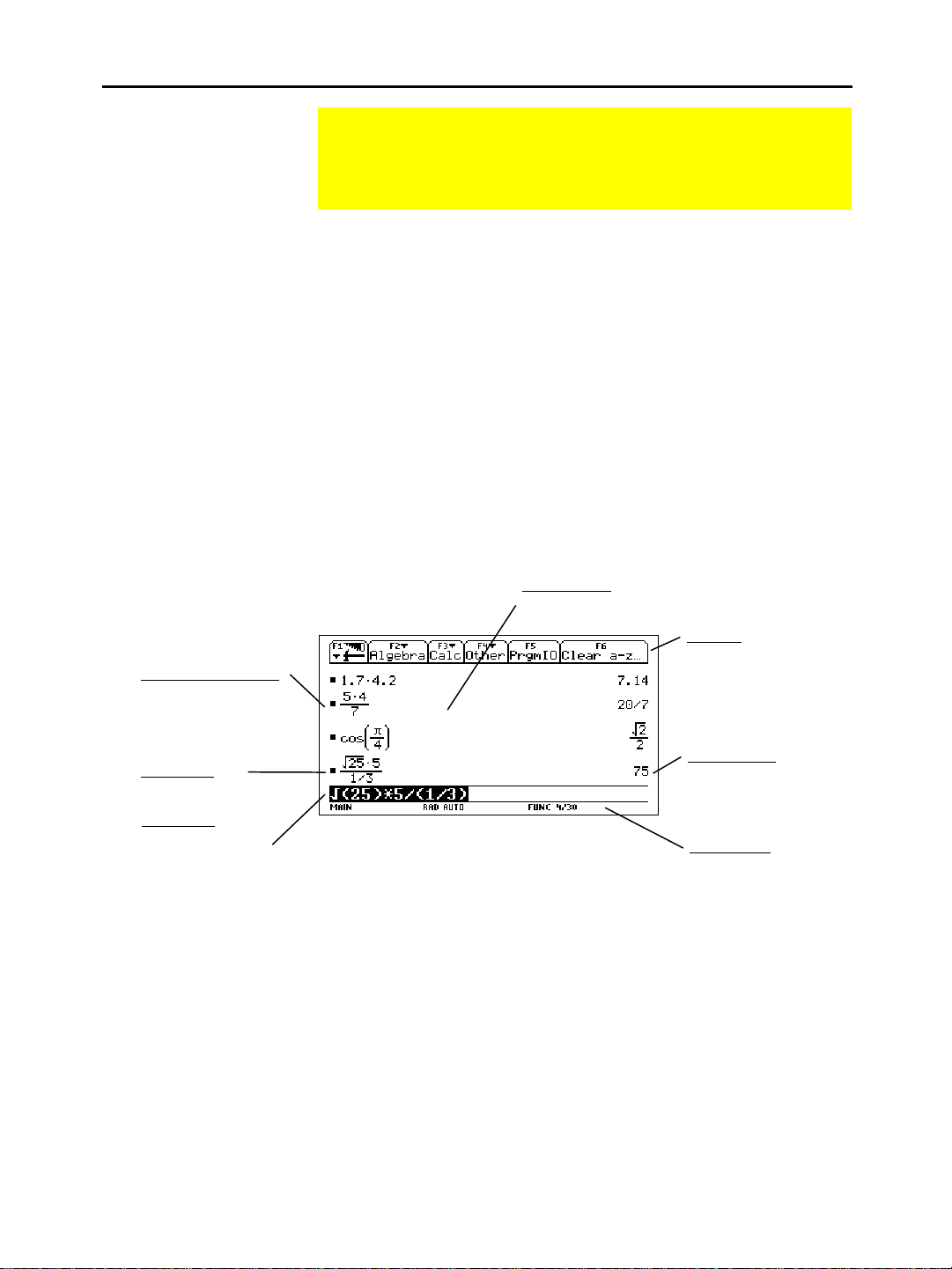
Home Screen
Displaying the Home Screen
Parts of the Home Screen
Pretty Print Display
Shows exponents,
roots, fractions, etc.,
in traditional form.
Refer to page 25.
Last Entry
Your last entry.
Entry Line
Where you enter
expressions or
instructions.
When you first turn on your
, the Home screen is
TI-92
displayed. The Home screen lets you execute instructions,
evaluate expressions, and view results.
When you turn on the
the display always shows the Home screen. (If the
after it has been turned off with 2 ®,
TI-92
turned itself
TI-92
off through APD, the display shows the previous screen, which may
or may not have been the Home screen.)
To display the Home screen at any time:
Press ¥ ".
¦
— or —
Press 2 K.
¦
— or —
Press O ¸ or O 1.
¦
The following example gives a brief description of the main parts of
the Home screen.
History Area
Lists entry/answer pairs
you have entered.
Toolbar
Press ƒ, „, etc., to
display menus for selecting
operations.
Last Answer
Result of your last entry.
Note that results are not
displayed on the entry line.
Status Line
Shows the current state
TI-92
of the
.
History Area
The history area shows up to eight previous entry/answer pairs
(depending on the complexity and height of the displayed
expressions). When the display is filled, information scrolls off the
top of the screen. You can use the history area to:
Review previous entries and answers. You can use the cursor to
¦
view entries and answers that have scrolled off the screen.
Recall or auto-paste a previous entry or answer onto the entry
¦
line so that you can re-use or edit it. Refer to pages 41 and 42.
Chapter 2: Operating the TI.92 19
Page 29

V
V
p
Home Screen
(Continued)
Scrolling through the History Area
Note: For an example of
viewing a long answer, refer
to page 24.
History Information on the Status Line
Normally, the cursor is in the entry line. However, you can move the
cursor into the history area.
To: Do this:
iew entries or answers
that have scrolled off
the screen
1. From the entry line, press C to
highlight the last answer.
2. Continue using C to move the
cursor from answer to entry, up
through the history area.
iew an entry or answer
that is too long for one
line (ú is at end of line)
Move the cursor to the entry or answer.
Use B and A to scroll left and right
(or 2 B and 2 A to go to the end
or the beginning), respectively.
Return the cursor to the
entry line
Press N, or press D until the cursor
is back on the entry line.
Use the history indicator on the status line for information about the
entry/answer pairs. For example:
If the cursor
is on the
entry line:
Total number of
pairs that are
currently saved.
8/30
Maximum number
of pairs that can
be saved.
Modifying the History Area
If the cursor
is in the
history area:
Pair number of
the highlighted
entry or answer.
Total number of
pairs that are
currently saved.
By default, the last 30 entry/answer pairs are saved. If the history
area is full when you make a new entry (indicated by
30/30
), the new
entry/answer pair is saved and the oldest pair is deleted. The history
indicator does not change.
To: Do this:
Change the number of
airs that can be saved
Press ƒ and select
¥
. Then press B, use C or D to
F
9:Format
, or press
highlight the new number, and press
¸ twice.
Clear the history area
and delete all saved pairs
Delete a particular
entry/answer pair
Press ƒ and select
ClrHome
enter
8:Clear Home
on the entry line.
Move the cursor to either the entry or
answer. Press 0 or M.
, or
20 Chapter 2: Operating the TI.92
Page 30
p
Entering Numbers
·
Entering a Negative Number
Important: Use | for
subtraction and use
for negation.
The
’s keypad lets you enter positive and negative
TI-92
numbers for your calculations. You can also enter numbers in
scientific notation.
1. Press the negation key ·. (Do not use the subtraction key |.)
2. Type the number.
To see how the
evaluates a negation in relation to other
TI-92
functions, refer to the Equation Operating System (EOS) hierarchy in
Appendix B. For example, it is important to know that functions
such as
Use c and d to include
ñ are evaluated before negation.
x
Evaluated as ë(2ñ)
arentheses if you have
any doubt about how a
negation will be
evaluated.
If you use | instead of · (or vice versa), you may get an error
message or you may get unexpected results. For example:
¦ 9
p ·
ë
=
63
7
— but —
p |
9
displays an error message.
7
Entering a Number in Scientific Notation
|
¦ 6
=
2
4
— but —
6 · 2 = ë12
·
¦
2 « 4 = 2
since it is interpreted as
, implied multiplication.
6(ë2)
— but —
|
subtracts 2 from the previous answer and then adds 4.
2 « 4
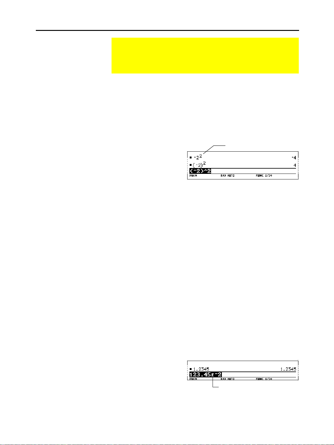
1. Type the part of the number that precedes the exponent. This
value can be an expression.
E
2. Press 2 ^.
appears in the display.
3. Type the exponent as an integer with up to 3 digits. You can use a
negative exponent.
Entering a number in scientific notation does not cause the answers
to be displayed in scientific or engineering notation.
The display format is
determined by the mode
settings (pages 25
through 27) and the
magnitude of the
Represents 123.45 × 10
-2
number.
Chapter 2: Operating the TI.92 21
Page 31

Entering Expressions and Instructions
You perform a calculation by evaluating an expression. You
initiate an action by executing the appropriate instruction.
Expressions are calculated and results are displayed
according to the mode settings described on page 25.
Definitions
Note: Appendix A describes
all of the
functions and instructions.
Note: This guidebook uses
the word command as a
generic reference to both
functions and instructions.
TI-92
’s built-in
Expression Consists of numbers, variables, operators, functions,
and their arguments that evaluate to a single answer.
ñ+
p
For example:
Enter an expression in the same order that it
¦
.
r
3
normally is written.
In most places where you are required to enter a
¦
value, you can enter an expression.
Operator Performs an operation such as +, ì, ù, ^.
Operators require an argument before and after the
¦
operator. For example:
4+5
and
5^2
.
Function Returns a value.
Functions require one or more arguments
¦
(enclosed in parentheses) after the function. For
example:
‡
(5)
and
min
(5,8)
.
Instruction Initiates an action.
Instructions cannot be used in expressions.
¦
Some instructions do not require an argument. For
¦
example:
Some require one or more arguments. For
¦
example:
ClrHome
Circle
.
.
0,0,5
For instructions, do not put the
arguments in parentheses.
The
Implied Multiplication
22 Chapter 2: Operating the TI.92
TI-92
conflict with a reserved notation.
Valid
Invalid
recognizes implied multiplication, provided it does not
If you enter: The
p
2
4 sin(46) 4ùsin(46)
or
5(1+2)
[1,2]a [a 2a]
2(a) 2ùa
xy
a(2)
a[1,2]
(1+2)5 5ù(1+2)
TI-92
interprets it as:
ùp
2
or
(1+2)ù5
Single variable named
xy
Function call
Matrix index to element
a[1,2]
Page 32

Parentheses
Expressions are evaluated according to the Equation Operating
System (EOS) hierarchy described in Appendix B. To change the
order of evaluation or just to ensure that an expression is evaluated
in the order you require, use parentheses.
Calculations inside a pair of parentheses are completed first. For
example, in
answer by
4(1+2)
.
4
, EOS first evaluates
and then multiplies the
(1+2)
Entering an Expression
Example
Type the expression, and then press ¸ to evaluate it. To enter a
function or instruction name on the entry line, you can:
¦
Press its key, if available. For example, press W.
— or —
¦
Select it from a menu, if available. For example, select
the
Number
submenu of the
MATH
menu.
2:abs
from
— or —
¦
Type the name letter-by-letter from the keyboard. You can use
any mixture of uppercase or lowercase letters. For example,
sin(
type
Calculate
3.76 e c · 7.9
2 ]
5 d
«
2 LOG c 45
3.76 ÷ (ë7.9 + ‡5) + 2 log 45
d
or
d
Sin(
«
.
.
3.76/(ë7.9+‡(
2 ]
inserts “‡( ”
because its argument
must be in parentheses.
3.76/(ë7.9+‡(5))
Use d once to close
‡
(5) and again to
ë
close (
3.76/(ë7.9+‡(5))+2log(45)
7.9 + ‡5).
Entering Multiple Expressions on a Line
Type the function
name.
¸
To enter more than one
expression or instruction
at a time, separate them
with a colon by pressing
2 Ë.
log
requires ( ) around
its argument.
Displays the last result only.
!
is displayed when you press
to store a value to a variable.
Chapter 2: Operating the TI.92 23
§
Page 33

A
Entering Expressions and Instructions
(Continued)
If an Entry or Answer Is Too Long for One Line
Note: When you scroll to
the right, 7 is displayed at
the beginning of the line.
Continuing a Calculation
In the history area, if both the entry and its answer cannot be
displayed on one line, the answer is displayed on the next line.
If an entry or answer is
too long to fit on one line,
ú is displayed at the end
of the line.
To view the entire entry or answer:
1. Press C to move the cursor from the entry line up into the
history area. This highlights the last answer.
2. As necessary, use C and D to highlight the entry or answer you
want to view. For example, C moves from answer to entry, up
through the history area.
3. Use B and A or
2 B and 2 A to
scroll right and left.
4. To return to the entry line, press N.
When you press ¸ to evaluate an expression, the
TI-92
leaves the
expression on the entry line and highlights it. You can continue to
use the last answer or enter a new expression.
Example
Stopping a Calculation
If you press: The
«, |, p, e,
Z, or §
TI-92
:
Replaces the entry line with the variable
which lets you use the last answer as the
beginning of another expression.
ny other key Erases the entry line and begins a new entry.
Calculate
3.76 e c · 7.9
2 ]
«
2 LOG c 45
¸
3.76 ÷ (ë7.9 + ‡5)
«
5 d d
¸
d
When a calculation is in progress, the
. Then add
When you press «, the entry line is replaced
with the variable ans(1), which contains the
last answer.
2 log 45
BUSY
to the result.
indicator appears on the
right end of the status line. To stop the calculation, press ´.
There may be a delay before the
“break” message is displayed.
Press N to return to the current
application.
ans(1)
,
24 Chapter 2: Operating the TI.92
Page 34

Formats of Displayed Results
A result may be calculated and displayed in any of several
formats. This section describes the
settings that affect the display formats. To check or change
your current mode settings, refer to page 35.
modes and their
TI-92
Pretty Print Mode
Exact/Approx Mode
Note: By retaining fractional
and symbolic forms,
reduces rounding errors that
could be introduced by
intermediate results in
chained calculations.
EXACT
By default,
Pretty Print = ON
. Exponents, roots, fractions, etc., are
displayed in the same form in which they are traditionally written.
You can use 3 to turn pretty print off and on.
Pretty Print
ON OFF
p
ñ
p
,
xì3
,
2
2
p
p
‡
,
,
^2
/2
((xì3)/2)
The entry line does not show an expression in pretty print. If pretty
print is turned on, the history area will show both the entry and its
result in pretty print after you press ¸.
By default,
Exact/Approx = AUTO
. You can use 3 to select from
three settings.
Because
is a combination of
AUTO
the other two settings, you should be
familiar with all three settings.
EXACT
fractional or symbolic form (
— Any result that is not a whole number is displayed in a
, p, 2, etc.).
1/2
Shows whole-number
results.
Shows simplified
fractional results.
Shows symbolic p.
Shows symbolic form
of roots that cannot
be evaluated to a
whole number.
EXACT
¸
setting
to
Press ¥
temporarily override
the
and display a floatingpoint result.
Chapter 2: Operating the TI.92 25
Page 35

Formats of Displayed Results
(Continued)
Exact/Approx Mode
(Continued)
Note: Results are rounded
to the precision of the
and displayed according to
current mode settings.
Tip: To retain an
form, use fractions instead
of decimals. For example,
use 3/2 instead of 1.5.
TI-92
EXACT
APPROXIMATE
— All numeric results, where possible, are displayed
in floating-point (decimal) form.
Because undefined variables cannot be evaluated, they are
treated algebraically. For example, if the variable
prñ
= 3.14159⋅r
AUTO
— Uses the
APPROXIMATE
certain functions may display
ñ
.
form where possible, but uses the
EXACT
form when your entry contains a decimal point. Also,
APPROXIMATE
results even if your
r
entry does not contain a decimal point.
Fractional
results are
evaluated
numerically.
Symbolic forms,
where possible,
are evaluated
numerically.
is undefined,
A decimal in the
entry forces a
floating-point
result.
The following chart compares the three settings.
Entry
8/4 2 2. 2
Tip: To evaluate an entry in
APPROXIMATE
regardless of the current
setting, press ¥
form,
¸
.
26 Chapter 2: Operating the TI.92
8/6 4/3 1.33333 4/3
8.5ù3 51/2 25.5 25.5
‡
(2)/2
pù
22
pù
2. 2
Exact
Result
2
2
⋅p
⋅p
Approximate
Result
.707107
6.28319 2
6.28319 6.28319
Auto
Result
2
A decimal in the
entry forces a
floating-point
2
result in
AUTO
.
⋅p
Page 36

Display Digits Mode
By default,
Display Digits = FLOAT 6
, which means that results are
rounded to a maximum of six digits. You can use 3 to select
different settings. The settings apply to all exponential formats.
Note: Regardless of the
Display Digits setting, the
full value is used for internal
floating-point calculations to
ensure maximum accuracy.
Note: A result is
automatically shown in
scientific notation if its
magnitude cannot be
displayed in the selected
number of digits.
Exponential Format Mode
Internally, the
calculates and retains all decimal results with up
TI-92
to 14 significant digits (although a maximum of 12 are displayed).
Setting Example Description
FIX
(0 – 12)
FLOAT 123.456789012
123. (FIX 0)
123.5 (FIX 1)
123.46 (FIX 2)
123.457 (FIX 3)
Results are rounded to the
selected number of decimal
places.
Number of decimal places varies,
depending on the result.
FLOAT
(1 – 12)
By default,
1.E 2 (FLOAT 1)
E
1.2
2 (FLOAT 2)
123. (FLOAT 3)
123.5 (FLOAT 4)
123.46 (FLOAT 5)
123.457 (FLOAT 6)
Exponential Format = NORMAL
Results are rounded to the total
number of selected digits.
.
You can use 3 to select from three
settings.
Note: In the history area, a
number in an entry is
displayed in
its absolute value is less
than .001.
SCIENTIFIC
if
Setting Example Description
NORMAL 12345.6
If a result cannot be displayed in the
number of digits specified by the
Display Digits
switches from
SCIENTIFIC
SCIENTIFIC 1.23456E 4 1.23456 × 10
Exponent (power of 10).
Always 1 digit to the left of the
decimal point.
E
ENGINEERING 12.3456
3 12.3456 × 10
Exponent is a multiple of 3.
May have 1, 2, or 3 digits to the
left of the decimal point.
Chapter 2: Operating the TI.92 27
mode, the
NORMAL
TI-92
to
for that result only.
4
3
Page 37

A
Editing an Expression in the Entry Line
Knowing how to edit an entry can be a real time-saver. If you
make an error while typing an expression, it’s often easier to
correct the mistake than to retype the entire expression.
Removing the Highlight from the Previous Entry
Moving the Cursor
Note: If you accidentally
press C instead of A or B,
the cursor moves up into the
history area. Press
press D until the cursor
returns to the entry line.
N
or
After you press ¸ to evaluate an expression, the
leaves that
TI-92
expression on the entry line and highlights it. To edit the expression,
you must first remove the highlight; otherwise, you may clear the
expression accidentally by typing over it.
To remove the highlight,
move the cursor toward
the side of the expression
you want to edit.
B
moves the cursor to the
end of the expression.
A
moves the cursor to the beginning.
After removing the highlight, move the cursor to the applicable
position within the expression.
To move the cursor: Press:
Left or right within an expression. A or B Hold the pad to
repeat the
movement.
To the beginning of the expression.
To the end of the expression.
2 A
2 B
Deleting a Character
To delete: Press:
The character to the
0 Hold 0 to delete multiple
left of the cursor.
The character to the
¥ 0
characters.
right of the cursor.
ll characters to the
right of the cursor.
M
(once only)
If there are no characters to the
right of the cursor, M erases
the entire entry line.
Clearing the Entry Line
To clear the entry line, press:
M if the cursor is at the beginning or end of the entry line.
¦
— or —
M M if the cursor is not at the beginning or end of the
¦
entry line. The first press deletes all characters to the right of the
cursor, and the second clears the entry line.
28 Chapter 2: Operating the TI.92
Page 38

Inserting or Overtyping a Character
Tip: Look at the cursor to
see if you’re in insert or
overtype mode.
The
TI-92
has both an insert and an overtype mode. By default, the
TI-92
is in the insert mode. To toggle between the insert and overtype
modes, press 2 /.
TI-92
If the
is in: The next character you type:
Will be inserted at the cursor.
Thin cursor between
characters
Will replace the highlighted
Cursor highlights a
character
character.
Replacing or Deleting Multiple Characters
Tip: When you highlight
characters to replace,
remember that some
function keys automatically
add an open parenthesis.
For example, pressing
types
cos(
.
X
First, highlight the applicable characters. Then, replace or delete all
the highlighted characters.
To: Do this:
Highlight multiple
characters
1. Move the cursor to either side of the
characters you want to highlight.
To replace
cursor beside
sin
with
sin
.
cos
, place the
2. Hold ¤ and press A or B to highlight
characters left or right of the cursor.
Hold ¤ and press B B B.
Replace the
Type the new characters.
highlighted
characters
— or —
Type COS.
Delete the
highlighted
characters
Press 0.
Chapter 2: Operating the TI.92 29
Page 39

A
TI.92
Menus
Displaying a Menu
To leave the keyboard uncluttered, the
uses menus to
TI-92
access many operations. This section gives an overview of
how to select an item from any menu. Specific menus are
described in the appropriate chapters of this guidebook.
Press: To display:
ƒ, „,
etc.
toolbar menu — Drops down from the toolbar at the
top of most application screens. Lets you select
operations useful for that application.
O
2 ¿
APPLICATIONS
of
CHAR
applications. Refer to page 33.
TI-92
menu — Lets you select from categories of
menu — Lets you select from the list
special characters (Greek, math, etc.).
2 I
menu — Lets you select from categories of
MATH
math operations.
2 ½
CATALOG
alphabetic list of the
menu — Lets you select from a complete,
’s built-in functions and
TI-92
instructions.
Selecting an Item from a Menu
To select an item from the displayed menu, either:
Press the number or letter shown to the left of that item.
¦
— or —
Use the cursor pad D and C to highlight the item, and then press
¦
¸. (Note that pressing C from the first item does not move
the highlight to the last item, nor vice versa.)
6
indicates that a menu will drop down
from the toolbar when you press „.
To select
This closes the menu and inserts the
function at the cursor location.
Selecting items marked with ú or . . . displays a
submenu or dialog box, respectively.
factor
factor(
, press 2 or D
¸
.
30 Chapter 2: Operating the TI.92
Page 40

Items Ending with ú
(Submenus)
If you select a menu item ending with ú, a submenu is displayed. You
then select an item from the submenu.
Items Containing “. . .” (Dialog Boxes)
For example,
submenu that lets you select a
specific List function.
ï
indicates that you can use
the cursor pad to scroll down
for additional items.
List
displays a
For items that have a submenu, you can use the cursor pad as
described below.
¦
To display the submenu for the highlighted item, press B.
(This is the same as selecting that item.)
¦
To cancel the submenu without making a selection, press A.
(This is the same as pressing N.)
If you select a menu item containing “
” (ellipsis marks), a dialog
. . .
box is displayed for you to enter additional information.
For example,
displays a dialog box that prompts
you to enter a folder name and a
variable name.
Save Copy As ...
"
indicates that you can press B to
display and select from a menu.
An input box indicates that you
must type a value.
After typing in an input box such as Variable, you must
¸
press
dialog box.
twice to save the information and close the
Chapter 2: Operating the TI.92 31
Page 41

TI.92
Menus
(Continued)
Keyboard Shortcuts
Moving from One Toolbar Menu to Another
Canceling a Menu
You can select certain menu items directly from the keyboard,
without first having to display a menu. If an item has a keyboard
shortcut, it is indicated on the menu.
Without even displaying this
menu, you can press ¥ S
to select
Save Copy As
.
To move from one toolbar menu to another without making a
selection, either:
¦
Press the key (ƒ, „, etc.) for the other toolbar menu.
— or —
¦
Use the cursor pad to move to the next (press B) or previous
(press A) toolbar menu. Pressing B from the last menu moves
to the first menu, and vice versa.
When using B, be sure that an item with a submenu is not
highlighted. If so, B displays that item’s submenu instead of moving
to the next toolbar menu.
To cancel the current menu without making a selection, press N.
Depending on whether any submenus are displayed, you may need to
press N several times to cancel all displayed menus.
Example: Selecting a Menu Item
Round the value of p to three decimal places. Starting from a clear
entry line on the Home screen:
1. Press 2 I to display the
MATH
2. Press
submenu. (Or press ¸ since
the first item is automatically
highlighted.)
3. Press
D D and ¸.)
4. Press 2 T
and then
evaluate the
expression.
32 Chapter 2: Operating the TI.92
menu.
to display the
1
to select
3
b
3
to
¸
round
d
Number
. (Or press
Selecting the function in Step 3
automatically typed
the entry line.
round(
on
Page 42

Selecting an Application
From the
APPLICATIONS
Note: To cancel the menu
without making a selection,
press N.
Menu
The
has different applications that let you solve and
TI-92
explore a variety of problems. You can select an application
from a menu, or you can access commonly used applications
directly from the keyboard.
1. Press O to display a menu that lists the applications.
2. Select an application. Either:
¦
Use the cursor pad D or C to
highlight the application and
.
then press
¸
— or —
¦
Press the number for that
application.
Application: Lets you:
Home
Enter expressions and instructions, and
perform calculations.
Y= Editor
Define, edit, and select functions or
equations for graphing (Chapter 3 and
Chapters 11 – 15).
Window Editor
Graph
Table
Data/Matrix Editor
Program Editor
Geometry
Text Editor
Set window dimensions for viewing a graph
(Chapter 3).
Display graphs (Chapter 3).
Display a table of variable values that
correspond to an entered function
(Chapter 4).
Enter and edit lists, data, and matrices. You
can perform statistical calculations and
graph statistical plots (Chapters 8 and 9).
Enter and edit programs and functions
(Chapter 17).
Construct geometric objects, and perform
analytical and transformational operations
(Chapter 7).
Enter and edit a text session (Chapter 16).
Chapter 2: Operating the TI.92 33
Page 43

Selecting an Application
e
(Continued)
From the Keyboard
Note: On your keyboard,
the application names abov
Q, W, etc., are printed in the
same color as the ¥ key.
You can access six commonly used applications from the
QWERTY
keyboard.
¥
1. Press the diamond (
2. Press the
Applications are
listed above the
QWERTY
QWERTY
keys.
Diamond key
) key.
key for the application.
For example, press ¥ and then Q to display the Home screen. This
guidebook uses the notation ¥ ", similar to the notation used
for second functions.
34 Chapter 2: Operating the TI.92
Page 44

Setting Modes
Modes control how numbers and graphs are displayed and
interpreted. Mode settings are retained by the Constant
Memoryé feature when the
is turned off. All numbers,
TI-92
including elements of matrices and lists, are displayed
according to the current mode settings.
Checking Mode Settings
Indicates you can
scroll down to see
additional modes.
Changing Mode Settings
Press 3 to display the
dialog box, which lists the modes
MODE
and their current settings.
There are two pages of mode
listings. Press ƒ or „ to quickly
display the first or second page.
Indicates that you can
press B or A to display
and select from a menu.
Modes that are not currently valid are dimmed. For example,
Note:
on the second page,
Split 2 App
is not valid when
Split Screen
=
FULL
When you scroll through the list, the cursor skips dimmed settings.
From the
MODE
dialog box:
1. Highlight the mode setting you want to change. Use D or C
(with ƒ and „) to scroll through the list.
2. Press B or A to display a menu that lists the valid settings. The
current setting is highlighted.
.
Tip: To cancel a menu and
return to the
box without making a
selection, press N.
MODE
dialog
3. Select the applicable setting. Either:
¦
Use D or C to highlight the setting and press ¸.
— or —
¦
Press the number or letter for that setting.
4. Change other mode settings, if necessary.
5. When you finish all your changes, press ¸ to save the
changes and exit the dialog box.
Important:
If you press N instead of ¸ to exit the
MODE
dialog box, any mode changes you made will be canceled.
Chapter 2: Operating the TI.92 35
Page 45

A
A
Setting Modes
(Continued)
Overview of the Modes
Note: For detailed
information about a
particular mode, look in the
applicable section of this
guidebook.
Mode Description
Graph
Current
Folder
Type of graphs to plot:
POLAR, SEQUENCE
Folder used to store and recall variables. Unless you
have created additional folders, only the
is available. Refer to “Using Folders to Store
Independent Sets of Variables” in Chapter 10.
Display
Digits
Maximum number of digits (
of decimal places (
result. Regardless of the setting, the total number of
displayed digits in a floating-point result cannot
exceed 12. Refer to page 27.
Angle
Units in which angle values are interpreted and
displayed:
Exponential
Format
Complex
Format
Notation used to display results:
SCIENTIFIC
Format used to display complex results, if any:
(complex results are not displayed unless you
REAL
use a complex entry),
Vector
Format
Format used to display 2- and 3-element vectors:
RECTANGULAR, CYLINDRICAL
RADIAN
, or
or
ENGINEERING
FUNCTION, PARAMETRIC
, or 3D.
MAIN
) or fixed number
FLOAT
) displayed in a floating-point
FIX
DEGREE
.
NORMAL
,
. Refer to page 27.
RECTANGULAR
, or
, or
POLAR
SPHERICAL
,
folder
.
.
Pretty Print
Split Screen
Split 1 App
Split 2 App
Number of
Graphs
Graph 2
Split Screen
Ratio
Exact/Approx
Turns the pretty print display feature
OFF
or ON.
Refer to page 25.
Splits the screen into two parts and specifies how the
parts are arranged:
TOP-BOTTOM
, or
(no split screen),
FULL
LEFT-RIGHT
. Refer to Chapter 5.
pplication in the top or left side of a split screen. If
you are not using a split screen, this is the current
application.
pplication in the bottom or right side of a split
screen. This is active only for a split screen.
For a split screen, lets you set up both sides of the
screen to display independent sets of graphs.
If
Number of Graphs = 2
, selects the type of graph in
the Split 2 part of the screen. Refer to Chapter 15.
Proportional sizes of the two parts of a split screen:
1:1, 1:2
, or
2:1
.
Calculates expressions and displays results in
numeric form or in rational/symbolic form:
EXACT
, or
APPROXIMATE
. Refer to page 25.
AUTO
,
36 Chapter 2: Operating the TI.92
Page 46

Using the Catalog to Select a Command
Selecting from the
CATALOG
Note: The first time you
display the
starts at the top of the list.
The next time you display
the
the same place you left it.
Tip: From the top of the list,
press C to move to the
bottom. From the bottom,
press D to move to the top.
CATALOG
CATALOG
, it
, it starts at
The
CATALOG
and instructions) on the
available on various menus, the
is an alphabetic list of all commands (functions
. Although the commands are
TI-92
CATALOG
lets you access any
command from one convenient list. It also gives help
information that describes a command’s parameters.
When you select a command, its name is inserted in the entry line at
the cursor location. Therefore, you should position the cursor as
necessary before selecting the command.
1. Press 2 ½.
¦
Commands are listed in alphabetical
order. Commands that do not start
with a letter (+, %, ‡, G, etc.) are at the
end of the list.
¦
To exit the
CATALOG
without
selecting a command, press N.
2. Move the ú indicator to the command, and press ¸.
To move the ú indicator: Press or type:
One command at a time D or C
One page at a time 2 D or 2 C
To the first command that
begins with a specified letter
The letter. For example, type
to go to the
Zoom
commands.
Z
Help Information about Parameters
Note: For details about the
parameters, refer to that
command’s description in
Appendix A.
For the command indicated by ú, the status line shows the required
and optional parameters, if any, and their type.
Indicated command
and its parameters
Brackets [ ] indicate
optional parameters.
From the example above, the syntax for
factor
expression
(
)
required
factor
is:
— or —
factor
expression,variable
(
optional
)
Chapter 2: Operating the TI.92 37
Page 47

Storing and Recalling Variable Values
When you store a value, you store it as a named variable. You
can then use the name instead of the value in expressions.
When the
substitutes the variable’s stored value.
encounters the name in an expression, it
TI-92
Rules for Variable Names
Examples
A variable name:
¦
Can use 1 to 8 characters consisting of letters and digits. This
includes Greek letters (but not p), accented letters, and
international letters. Do not include spaces.
− The first character cannot be a digit.
¦
Can use uppercase or lowercase letters. The names
, and
aB22
¦
Cannot be the same as a name that is preassigned by the
all refer to the same variable.
ab22
AB22, Ab22
Preassigned names include:
abs
− Built-in functions (such as
LineVert
). Refer to Appendix A.
− System variables (such as
) and instructions (such as
xmin
and
, which are used to
xmax
store graph-related values). Refer to Appendix B for a list.
Variable Description
myvar
a
Log
Log1
3rdTotal
circumfer
OK.
OK.
Not OK, name is preassigned to the
OK.
Not OK, starts with a digit.
Not OK, more than 8 characters.
log
function.
TI-92
,
.
Data Types
You can save any
types, refer to
Data Types Examples
Expressions
Lists
Matrices
Character strings
Pictures
Functions
38 Chapter 2: Operating the TI.92
TI-92
getType()
data type as a variable. For a list of data
in Appendix A. Some examples are:
2.54, 1.25í6, 2p, xmin/10, 2+3i, (xì2)ñ, 2/2
{2 4 6 8}, {1 1 2}
1 0 0
[]
,
[1 0 0]
“Hello”, “The answer is:”, “xmin/10”
myfunc(arg), ellipse(x,y,r1,r2)
3 4 6
Page 48

v
p
Storing a Value in a
g
n
Variable
1. Enter the value you want to store, which can be an expression.
2. Press §. The store symbol (!) is displayed.
3. Type the variable
name.
4. Press ¸.
To store to a variable temporarily, you can use the “with” operator.
Refer to “Substituting Values and Setting Constraints” in Chapter 6.
Displaying a Variable
Note: Refer to Chapter 6 for
information about symbolic
manipulation.
Using a Variable in an Expression
Tip: To view a list of existin
variable names, use
2 °
Chapter 18.
as described i
1. Type the variable
name.
2. Press ¸.
If the variable is undefined, the variable name is shown in the result.
In this example, the
ariable a is undefined.
Therefore, it is used as a
symbolic variable.
1. Type the variable
name into the
expression.
2. Press ¸ to
evaluate the
The variable’s value
did not change.
expression.
If you want the result to
replace the variable’s
revious value, you must
store the result.
Recalling a Variable’s Value
In some cases, you may want to use a variable’s actual value in an
expression instead of the variable name.
1. Press 2 £ to
display a dialog box.
2. Type the variable
name.
3. Press ¸ twice.
In this example, the value stored in
will be inserted at the
num1
cursor position in the entry line.
Chapter 2: Operating the TI.92 39
Page 49

Reusing a Previous Entry or the Last Answer
y
e
You can reuse a previous entry by reexecuting the entry
“as is” or by editing the entry and then reexecuting it. You can
also reuse the last calculated answer by inserting it into a new
expression.
Reusing the Expression on the Entry Line
Tip: Reexecuting an entry
“as is” is useful for iterative
calculations that involve
variables.
Tip: Editing an entry lets
ou make minor changes
without retyping the entire
entry.
When you press
¸
to evaluate an expression, the
TI-92
leaves that
expression on the entry line and highlights it. You can type over the
entry, or you can reuse it as necessary.
For example, using a variable, find the square of
1, 2, 3
, etc.
1. Set the initial variable value.
0
§
NUM
¸
2. Enter the variable
expression.
UM « 1 § NUM
N
2
ã:ä NUM Z 2
¸
3. Reenter to increment
the variable and
calculate the square.
¸
¸
Using the equation
2
, use trial and error to find the radius of a
A=pr
circle that covers 200 square centimeters.
1. Use
as your first
8
guess.
§
8
2 ãpä
R 2 ã:
R
Z
2
ä
¸
2. Display the answer in
its approximate
floating-point form.
¥ ¸
Note: When the entry
contains a decimal point, th
result is automatically
displayed in floating-point.
3. Edit and reexecute
7.95
¸
.
with
A ¥ 0
7.95
4. Continue until the answer is as accurate as you want.
40 Chapter 2: Operating the TI.92
Page 50

r
Recalling a Previous Entry
Note: You can also use the
entry function to recall any
previous entry. Refer to
entry() in Appendix A.
You can recall any previous entry that is stored in the history area,
even if the entry has scrolled off the top of the screen. The recalled
entry replaces whatever is currently shown on the entry line. You can
then reexecute or edit the recalled entry.
To recall: Press: Effect:
The last entry
(if you’ve changed
the entry line)
Previous entries 2 ²
2 ²
once
repeatedly
If the last entry is still shown on
the entry line, this recalls the
entry prior to that.
Each press recalls the entry prio
to the one shown on the entry
line.
For example:
Recalling the Last Answer
Note: Refer to ans() in
Appendix A.
If the entry line contains
the last entry, 2
recalls this entry.
If the entry line is edited
or cleared, 2
recalls this entry.
Each time you evaluate an expression, the
the variable
²
²
stores the answer to
TI-92
. To insert this variable in the entry line, press
ans(1)
2 ±.
For example, calculate the area of a garden plot that is 1.7 meters by
4.2 meters. Then calculate the yield per square meter if the plot
produces a total of 147 tomatoes.
1. Find the area.
¸
p
1.7
4.2
2. Find the yield.
147 e 2 ±
Just as
ans(1)
also contain previous answers. For example,
¸
Variable ans(1) is inserted,
and its value is used in the
calculation.
always contains the last answer,
ans(2), ans(3)
contains the
ans(2)
, etc.,
next-to-last answer.
Chapter 2: Operating the TI.92 41
Page 51

I
R
v
p
Auto-Pasting an Entry or Answer from the History Area
ƒ
You can select any entry or answer from the history area and
“auto-paste” a duplicate of it on the entry line. This lets you
insert a previous entry or answer into a new expression
without having to retype the previous information.
Why Use Auto-Paste
Note: You can also paste
information by using the
toolbar menu. Refer to
“Cutting, Copying, and
Pasting Information” in
Chapter 10.
Auto-Pasting an Entry or Answer
Tip: To cancel auto-paste
and return to the entry line,
press N.
Tip: To view an entry or
answer too long for one line
(indicated by ú at the end of
the line), use
and
2 B
and A or
B
2 A
.
The effect of using auto-paste is similar to 2 ² and 2 ± as
described in the previous section, but there are differences.
For entries:
For answers:
Pasting lets you: 2 ² lets you:
nsert any previous
entry into the entry
line.
Pasting lets you: 2 ± lets you:
Insert the displayed
alue of any
revious answer
into the entry line.
eplace the contents of the
entry line with any previous
entry.
Insert the variable
which contains the last
answer only. Each time you
enter a calculation,
ans(1)
ans(1)
,
is
updated to the latest answer.
1. On the entry line, place the cursor where you want to insert the
entry or answer.
2. Press C to move the cursor up into the history area. This
highlights the last answer.
3. Use C and D to highlight the entry or answer to auto-paste.
C moves from
¦
answer to entry
up through the
history area.
¦
You can use C to
highlight items
that have scrolled
off the screen.
4. Press ¸.
The highlighted item
is inserted in the
entry line.
This pastes the entire entry or answer. If you need only a part of the
entry or answer, edit the entry line to delete the unwanted parts.
42 Chapter 2: Operating the TI.92
Page 52

y
A
A
A
A
Status Line Indicators in the Display
The status line is displayed at the bottom of all application
screens. It shows information about the current state of the
, including several important mode settings.
TI-92
Status Line Indicators
Current
Folder
Indicator Meaning
Modifier
Current
Folder
Key
Angle
Mode
Exact/Approx
Mode
Shows the name of the current folder. Refer to
“Using Folders to Store Independent Sets of
Variables” in Chapter 10.
Graph
Number
Graph
Mode
History
Pairs
is the default folder
MAIN
that is set up automatically when you use the
Modifier Key Displayed when you press ¤, ¥, 2, or ‚.
+
The
will type an uppercase character for the
TI-92
next letter key you press.
2
The
will access the diamond feature of the next
TI-92
key you press.
2ND
The
will use the second function of the next ke
TI-92
you press.
∂
When used in combination with the cursor pad, the
will use any “dragging” features that are
TI-92
available in graphing and geometry.
Battery
Indicator
Busy
Indicator
TI-92
.
ngle
Mode
Shows the units in which angle values are interpreted
and displayed. To change the
mode, use the
Angle
3 key.
RAD
DEG
Exact/
pprox
Mode
AUTO
EXACT
APPROX
Radians
Degrees
Shows how answers are calculated and displayed.
Refer to page 25. To change the
Exact/Approx
use the 3 key.
uto
Exact
pproximate
Chapter 2: Operating the TI.92 43
mode,
Page 53

A
Status Line Indicators in the Display
(Continued)
Status Line Indicators
(Continued)
Indicator Meaning
Graph
Number
Graph
Mode
FUNC y(x)
PAR x(t)
POL r(q)
SEQ u(n)
3D z(x,y)
History
Pairs
If the screen is split to show two independent graphs,
this indicates which graph is active (
Indicates the type of graphs that can be plotted. (To
change the
functions
and
polar equations
sequences
3D equations
Displayed only on the Home screen to show
information about the number of entry/answer pairs
in the history area. Refer to page 20.
Battery
Indicator
Displayed only when the batteries are getting low.
If
BATT
the batteries as soon as possible.
Busy
Indicator
Displayed only when the
calculation or plotting a graph.
or
mode, use the 3 key.)
Graph
parametric equations
y(t)
GR#1
GR#2
is shown with a black background, change
is performing a
TI-92
).
BUSY
PAUSE
calculation or graph is in progress.
You have paused a graph or program.
44 Chapter 2: Operating the TI.92
Page 54

Chapter 3: Basic Function Graphing
Preview of Basic Function Graphing..................................................... 46
Overview of Steps in Graphing Functions............................................ 47
Setting the Graph Mode .......................................................................... 48
Defining Functions for Graphing ........................................................... 49
3
Selecting Functions to Graph................................................................. 51
Setting the Display Style for a Function ............................................... 52
Defining the Viewing Window................................................................ 53
Changing the Graph Format ................................................................... 54
Graphing the Selected Functions........................................................... 55
Displaying Coordinates with the Free-Moving Cursor........................ 56
Tracing a Function................................................................................... 57
Using Zooms to Explore a Graph........................................................... 59
Using Math Tools to Analyze Functions ............................................... 62
This chapter describes the steps used to display and explore a
graph. Before using this chapter, you should be familiar with
.
Chapter 2: Operating the
TI-92
Y= Editor shows
an algebraic
representation.
Graph screen
shows a graphic
representation.
Although this chapter describes how to graph
basic steps apply to all graphing modes. Later chapters give
specific information about the other graphing modes.
functions, the
y(x)
Chapter 3: Basic Function Graphing 45
Page 55

Preview of Basic Function Graphing
Graph a circle of radius 5, centered on the origin of the coordinate system. View the circle
using the standard viewing window (
ZoomStd
). Then use
window.
Steps Keystrokes Display
ZoomSqr
to adjust the viewing
1. Display the
For
mode, select
Graph
MODE
dialog box.
FUNCTION
.
2. Display the Home screen. Then store
the radius, 5, in variable
.
r
3. Display and clear the Y= Editor.
Then define
y1(x)
=
rñ - x
ñ
,
the top half of a circle.
In function graphing, you must define
separate functions for the top and bottom
halves of a circle.
4. Define
y2(x)
=
ë
rñ - x
ñ
, the function
for the bottom half of the circle.
The bottom half is the negative of the top
half, so you can define y2(x) = ëy1(x).
5. Select the
ZoomStd
viewing window,
which automatically graphs the
functions.
In the standard viewing window, both the
x and y axes range from ë10 to 10.
However, this range is spread over a longer
distance along the x axis than the y axis.
Therefore, the circle appears as an ellipse.
6. Select
ZoomSqr increases the range along the
x axis so that circles and squares are shown
in correct proportion.
ZoomSqr
.
3
B 1
¸
¥"
5§R¸
¥#
ƒ8¸
¸
2]RZ2|X
Z2d¸
¸
· Y1cXd
¸
„ 6
Notice slight gap
between top and
bottom halves.
„ 5
5!r5
Use the full function name
y1(x), not simply y1.
There is a gap between the top and bottom halves of the circle because each half is a
Note:
separate function. The mathematical endpoints of each half are (-5,0) and (5,0). Depending on
the viewing window, however, the plotted endpoints for each half may be slightly different from
their mathematical endpoints.
46 Chapter 3: Basic Function Graphing
Page 56

Overview of Steps in Graphing Functions
To graph one or more y(x) functions, use the general steps
shown below. For a detailed description of each step, refer to
the following pages. You may not need to do all the steps
each time you graph a function.
Graphing Functions
Set Graph mode (3)
FUNCTION
to
Also set Angle mode,
if necessary.
Define functions on
Y= Editor (¥ #).
.
Tip: To turn off any stat
data plots (Chapter 9),
press
deselect them.
Tip: This is optional. For
multiple functions, this helps
visually distinguish one from
another.
Tip:
the viewing window.
or use † to
‡
5
„ Zoom
also changes
Select (†) which
defined functions to
graph.
Set the display style
(ˆ) for a function.
Define the viewing
window (¥
Change the graph
format (¥ F or ƒ 9),
if necessary.
Graph the selected
functions (¥
$
%
).
).
Exploring the Graph
From the Graph screen, you can:
¦
Display the coordinates of any pixel by using the free-moving
cursor, or of a plotted point by tracing a function.
¦
Use the „
toolbar menu to zoom in or out on a portion of
Zoom
the graph.
¦
Use the ‡
toolbar menu to find a zero, minimum,
Math
maximum, etc.
Chapter 3: Basic Function Graphing 47
Page 57

Setting the Graph Mode
t
Graph Mode
For graphs that do no
Note:
use complex numbers, set
Complex Format =
Otherwise, it may affect
graphs that use powers,
such as x
1/3
REAL
.
Before graphing y(x) functions, you must select
graphing. You may also need to set the
affects how the
1. Press
3
to display the
graphs trigonometric functions.
TI-92
current mode settings.
2. Set the
Graph
mode to
Chapter 2.
.
While this chapter specifically describes
lets you select from five
TI-92
Graph Mode Setting Description
FUNCTION y(x)
MODE
FUNCTION
Graph
functions
FUNCTION
Angle
mode, which
dialog box, which shows the
. Refer to “Setting Modes” in
function graphs, the
y(x)
mode settings.
Other
Note:
settings are described in
later chapters.
Graph
mode
Angle Mode
Checking the Status Line
PARAMETRIC x(t)
POLAR r(q)
SEQUENCE u(n)
3D z(x,y)
and
polar equations
sequences
parametric equations
y(t)
3D equations
When using trigonometric functions, set the
(
RADIAN
or
DEGREE
) in which you want to enter and display angle
values.
To see the current
Graph
mode and
mode, check the status line
Angle
at the bottom of the screen.
Angle
Mode
mode for the units
Angle
Graph
Mode
48 Chapter 3: Basic Function Graphing
Page 58

Defining Functions for Graphing
y
Defining a New Function
Note: The function list
shows abbreviated function
names such as y1, but the
entry line shows the full
name y1(x).
Tip: For an undefined
function, you do not need to
press
ou begin typing, the cursor
moves to the entry line.
¸
or …. When
In
FUNCTION
graphing mode, you can graph functions named
y1(x) through y99(x). To define and edit these functions, use
the Y= Editor. (The Y= Editor lists function names for the
current graphing mode. For example, in
POLAR
graphing
mode, function names are r1(q), r2(q), etc.)
1. Press ¥ # or O 2 to display the Y= Editor.
Plots
— You can scroll
above y1= to see a list of
stat plots. See Chapter 9.
Function List
scroll through the list of
functions and definitions.
Entry Line
define or edit the function
highlighted in the list.
— You can
— Where you
2. Press D and C to move the cursor to any undefined function.
(Use 2 D and 2 C to scroll one page at a time.)
3. Press ¸ or … to move the cursor to the entry line.
4. Type the expression to define the function.
¦
The independent variable in function graphing is x.
¦
The expression can refer to other variables, including
matrices, lists, and other functions.
Tip: If you accidentally
move the cursor to the entry
line, press
back to the function list.
to move it
N
Editing a Function
5. When you complete the expression, press ¸.
The function list now shows the new function, which is
automatically selected for graphing.
From the Y= Editor:
1. Press D and C to highlight the function.
2. Press ¸ or … to move the cursor to the entry line.
3. Do any of the following.
¦
Use B and A to move the cursor within the expression and
edit it. Refer to “Editing an Expression in the Entry Line” in
Chapter 2.
— or —
¦
Press M once or twice to clear the old expression, and
then type the new one.
Tip: To cancel any editing
changes, press
of
¸
.
N
instead
4. Press ¸.
The function list now shows the edited function, which is
automatically selected for graphing.
Chapter 3: Basic Function Graphing 49
Page 59

A
A
A
Defining Functions for Graphing
y
(Continued)
Clearing a Function
Note:
any stat plots (Chapter 9).
does not erase
ƒ 8
From the Home Screen or a Program
Tip: User-defined functions
can have almost any name.
However, if you want them
to appear in the Y= Editor,
use function names
, etc.
2(x)
y1(x)
,
From the Y= Editor:
To erase: Do this:
function from
Highlight the function and press 0 or M.
the function list
function from
the entry line
ll functions Press ƒ and then select
Press M once or twice (depending on the
cursor’s location) and then press ¸.
8:Clear Functions
.
When prompted for confirmation, press ¸.
You don’t have to clear a function to prevent it from being graphed.
As described on page 51, you can select the functions you want to
graph.
You can also define and evaluate a function from the Home screen or
a program.
¦
Use the
Define
and
Graph
commands. Refer to:
− “Graphing a Function Defined on the Home Screen” and
“Graphing a Piecewise Defined Function” in Chapter 15.
− “Overview of Entering a Function” in Chapter 17.
¦
Store an expression directly to a function variable. Refer to:
− “Storing and Recalling Variable Values” in Chapter 2.
− “Creating and Evaluating User-Defined Functions” in
Chapter 10.
50 Chapter 3: Basic Function Graphing
Page 60

A
A
Selecting Functions to Graph
Regardless of how many functions are defined in the
Y= Editor, you can select the ones you want to graph.
Selecting or Deselecting Functions
Selected
Deselected
Tip: You don’t have to
select a function when you
enter or edit it; it is selected
automatically.
Tip: To turn off any stat
plots, press
to deselect them.
‡ 5
or use
†
Press ¥ # or O 2 to display the Y= Editor.
A “Ÿ” indicates which functions will be graphed the next time you
display the Graph screen.
PLOT
If
numbers are
displayed, those stat plots
are selected.
In this example, Plots 1
and 2 are selected. To
view them, scroll above
y1=.
To select or deselect: Do this:
specified function 1. Move the cursor to highlight the function.
2. Press †.
This procedure selects a deselected function
or deselects a selected function.
ll functions 1. Press ‡ to display the
All
toolbar menu.
2. Select the applicable item.
From the Home Screen or a Program
You can also select or deselect functions from the Home screen or a
program.
¦
Use the
screen’s †
FnOn
FnOff
and
Other
commands (available from the Home
toolbar menu) for functions. Refer to
Appendix A.
¦
Use the
PlotsOn
and
PlotsOff
commands for stat plots. Refer to
Appendix A.
Chapter 3: Basic Function Graphing 51
Page 61

A
A
Setting the Display Style for a Function
For each defined function, you can set a style that specifies
how that function will be graphed. This is useful when
graphing multiple functions. For example, set one as a solid
line, another as a dotted line, etc.
Displaying or Changing a Function’s Style
Tip: To set
for all functions, press
and select
as the style
Line
4:Reset Styles
‡
From the Y= Editor:
1. Move the cursor to highlight the applicable function.
2. Press ˆ.
¦
Although the
item is initially
Line
highlighted, the function’s current style is
indicated by a Ÿ mark.
¦
To exit the menu without making a
change, press N.
3. To make a change, select the applicable style.
Style Description
Line
Dot
.
Square
Thick
Animate
Connects plotted points with a line. This is the default.
Displays a dot at each plotted point.
Displays a solid box at each plotted point.
Connects plotted points with a thick line.
round cursor moves along the leading edge of the
graph but does not leave a path.
Path
round cursor moves along the leading edge of the
graph and does leave a path.
Shades the area above the graph.
Shades the area below the graph.
has four shading patterns, used on a rotating basis. If you
If You Use Above or Below Shading
Above
Below
The
TI-92
set one function as shaded, it uses the first pattern. The next shaded
function uses the second pattern, etc. The fifth shaded function
reuses the first pattern.
When shaded areas intersect,
their patterns overlap.
From the Home
Screen or a
You can also set a function’s style from the Home screen or a
Style
program. Refer to the
command in Appendix A.
Program
52 Chapter 3: Basic Function Graphing
Page 62

Defining the Viewing Window
The viewing window represents the portion of the coordinate
plane displayed on the Graph screen. By setting Window
variables, you can define the viewing window’s boundaries
and other attributes. Function graphs, parametric graphs, etc.,
have their own independent set of Window variables.
Displaying Window Variables in the Window Editor
Tip: To turn off tick marks,
set xscl=0 and/or yscl=0.
Tip: Small values of xres
improve the graph’s
resolution but may reduce
the graphing speed.
Press ¥ $ or O 3 to display the Window Editor.
ymax
xmin
yscl
Window Variables
(shown in Window Editor)
Variable Description
,
xmin, xmax
ymin, ymax
xscl, yscl
xres
Boundaries of the viewing window.
Distance between tick marks on the x and y axes.
Sets pixel resolution (1 through 10) for function graphs.
ymin
Corresponding Viewing Window
(shown on Graph screen)
The default is 2.
¦
At 1, functions are evaluated and graphed at each
pixel along the x axis.
¦
At 10, functions are evaluated and graphed at every
10th pixel along the x axis.
xscl
xmax
Changing the Values
Note: If you type an
expression, it is evaluated
when you move the cursor
to a different Window
variable or leave the
Window Editor.
From the Home Screen or a Program
From the Window Editor:
1. Move the cursor to highlight the value you want to change.
2. Do any of the following:
¦
Type a value or an expression. The old value is erased when
you begin typing.
— or —
¦
Press M to clear the old value; then type the new one.
— or —
¦
Press A or B to remove the highlighting; then edit the value.
Values are stored as you type them; you do not need to press ¸.
¸ simply moves the cursor to the next Window variable.
You can also store values directly to the Window variables from the
Home screen or a program. Refer to “Storing and Recalling Variable
Values” in Chapter 2.
Chapter 3: Basic Function Graphing 53
Page 63

Changing the Graph Format
N
You can set the graph format to show or hide reference
elements such as the axes, a grid, and the cursor’s
coordinates. Function graphs, parametric graphs, etc., have
their own independent set of graph formats.
Displaying Graph Format Settings
Tip: You also can press
from the Y= Editor,
¥ F
Window Editor, or Graph
screen.
Tip: To turn off tick marks,
define the viewing window
so that xscl and/or yscl = 0.
From the Y= Editor, Window Editor, or Graph screen, press ƒ and
select
9:Format
.
¦
The
GRAPH FORMATS
dialog
box shows the current
settings.
¦
To exit without making a
change, press N.
Format Description
Coordinates
Shows cursor coordinates in rectangular (
or polar (
POLAR
) form, or hides (
OFF
) the
RECT
coordinates.
Graph Order
Grid
Graphs functions one at a time (
same time (
Shows (ON) or hides (
SIMUL
).
) grid points that
OFF
) or all at the
SEQ
correspond to the tick marks on the axes.
Axes
Leading Cursor
Shows (ON) or hides (
Shows (ON) or hides (
) the x and y axes.
OFF
) a reference cursor
OFF
that tracks the functions as they are graphed.
)
Labels
Changing Settings
From the
GRAPH FORMATS
1. Move the cursor to highlight the format setting.
2. Press B to display a menu of valid settings for that format.
3. Select a setting. Either:
¦
Tip: To cancel a menu or
exit the dialog box without
saving any changes, use
instead of
¸
.
Move the cursor to highlight the setting, and then press ¸.
— or —
¦
Press the number for that setting.
4. After changing all applicable format settings, press ¸ to save
your changes and close the
54 Chapter 3: Basic Function Graphing
Shows (ON) or hides (
axes.
dialog box:
GRAPH FORMATS
) labels for the x and y
OFF
dialog box.
Page 64

Graphing the Selected Functions
When you are ready to graph the selected functions, display
the Graph screen. This screen uses the display style and
viewing window that you previously defined.
Displaying the Graph Screen
Note: If you select an
Zoom operation from the
Y= Editor or Window Editor,
the
displays the Graph screen.
automatically
TI-92
„
Interrupting Graphing
If You Need to Change the Viewing Window
Press ¥ % or O 4. The
automatically graphs the
TI-92
selected functions.
BUSY
indicator shows while
graphing is in progress.
While graphing is in progress:
To pause graphing temporarily, press ¸. (The
¦
indicator replaces
To cancel graphing, press ´. To start graphing again from the
¦
beginning, press † (
.) To resume, press ¸ again.
BUSY
ReGraph
).
PAUSE
Depending on various settings, a function may be graphed such that
it is too small, too large, or offset too far to one side of the screen. To
correct this:
Redefine the viewing window with different boundaries
¦
(page 53).
Smart Graph
Use a
¦
When you display the Graph screen, the
operation (page 59).
Zoom
Smart Graph
feature displays
the previous window contents immediately, provided nothing has
changed that requires regraphing.
Smart Graph
Changed a mode setting that affects graphing, a function’s
¦
updates the window and regraphs only if you have:
graphing attribute, a Window variable, or a graph format.
Selected or deselected a function or stat plot. (If you only select a
¦
new function,
Changed the definition of a selected function or the value of a
¦
Smart Graph
adds that function to the Graph screen.)
variable in a selected function.
Cleared a drawn object (Chapter 15).
¦
Changed a stat plot definition (Chapter 9).
¦
Chapter 3: Basic Function Graphing 55
Page 65

Displaying Coordinates with the Free-Moving Cursor
To display the coordinates of any location on the Graph
screen, use the free-moving cursor. You can move the cursor
to any pixel on the screen; the cursor is not confined to a
graphed function.
Free-Moving Cursor
Tip: If your screen does not
show coordinates, set the
graph format
Coordinates =
POLAR
Tip: To hide the cursor and
its coordinates temporarily,
press
The next time you move the
cursor, it moves from its last
position.
(¥ F)
RECT
.
M, N
so that
or
,
or
¸
When you first display the Graph screen, no cursor is visible. To
display the cursor, press the cursor pad. The cursor moves from the
center of the screen, and its coordinates are displayed.
y1(x)=xñ
The “c” indicates these are cursor
coordinates. The values are stored in
the xc and yc system variables.
Rectangular coordinates use xc and
yc. Polar coordinates use rc and qc.
To move the free-moving cursor: Press:
To an adjoining pixel The cursor pad for any
.
direction.
In increments of 10 pixels 2 and then the cursor pad.
When you move the cursor to a pixel that appears to be “on” the
function, it may be near the function but not on it.
Cursor coordinates are for
the center of the pixel, not
the function.
To increase the accuracy:
¦
Use the
Trace
coordinates that are on the function.
¦
56 Chapter 3: Basic Function Graphing
Use a
Zoom
tool described on the next page to display
operation to zoom in on a portion of the graph.
Page 66

A
Tracing a Function
To display the exact coordinates of any plotted point on a
graphed function, use the …
tool. Unlike the free-
Trace
moving cursor, the trace cursor moves only along a function’s
plotted points.
Beginning a Trace
Note: If any stat plots are
graphed (Chapter 9), the
trace cursor appears on the
lowest-numbered stat plot.
Moving along a Function
Note: If you enter an x
value, it must be between
xmin and xmax.
Tip: If your screen does not
show coordinates, set the
graph format
Coordinates =
POLAR
(¥ F)
so that
or
RECT
.
From the Graph screen, press ….
The trace cursor appears on the function, at the middle
value on
x
the screen. The cursor’s coordinates are displayed at the bottom of
the screen.
If multiple functions are graphed, the trace cursor appears on the
lowest-numbered function selected in the Y= Editor. The function
number is shown in the upper right part of the screen.
To move the trace cursor: Do this:
To the previous or next plotted point Press A or B.
pproximately 5 plotted points
Press 2 A or 2 B.
(it may be more or less than 5,
depending on the
Window variable)
xres
To a specified x value on the function Type the x value and
press ¸.
The trace cursor moves only from plotted point to plotted point
along the function, not from pixel to pixel.
Function number being traced.
For example: y1(x).
Trace coordinates are
those of the function, not
the pixel.
yn(x)
.
Tip: Use QuickCenter,
described on the next page,
to trace a function that goes
above or below the window.
Each displayed y value is calculated from the x value; that is, y=
x
If the function is undefined at an
value, the y value is blank.
You can continue to trace a function that goes above or below the
viewing window. You cannot see the cursor as it moves in that
“off the screen” area, but the displayed coordinate values show its
correct coordinates.
Chapter 3: Basic Function Graphing 57
Page 67

Tracing a Function
(Continued)
Moving from Function to Function
Automatic Panning
Note: Automatic panning
does not work if stat plots
are displayed or if a function
uses a shaded display style.
Using QuickCenter
Press C or D to move to the previous or next selected function at
the same
value. The new function number is shown on the screen.
x
The “previous or next” function is based on the order of the selected
functions in the Y= Editor, not the appearance of the functions as
graphed on the screen.
If you trace a function off the left or right edge of the screen, the
viewing window automatically pans to the left or right. There is a
slight pause while the new portion of the graph is drawn.
Before automatic pan After automatic pan
After an automatic pan, the cursor continues tracing.
If you trace a function off the top or bottom of the viewing window,
you can press ¸ to center the viewing window on the cursor
location.
Tip: You can use
QuickCenter at any time
during a trace, even when
the cursor is still on the
screen.
Canceling Trace
Before using QuickCenter After using QuickCenter
After
QuickCenter
, the cursor stops tracing. If you want to continue
tracing, press ….
To cancel a trace at any time, press N.
A trace is also canceled when you display another application screen
such as the Y= Editor. When you return to the Graph screen and
press … to begin tracing:
¦
¦
If
middle
If
Smart Graph
Smart Graph
regraphed the screen, the cursor appears at the
value.
x
does not regraph the screen, the cursor appears at
its previous location (before you displayed the other application).
58 Chapter 3: Basic Function Graphing
Page 68

A
A
A
Using Zooms to Explore a Graph
Overview of the Zoom Menu
Note: If you select a
tool from the Y=Editor or
Window Editor, the
automatically displays the
Graph screen.
Note: ∆
distances from the center of
one pixel to the center of an
adjoining pixel.
and ∆y are the
x
Zoom
TI-92
The „
Zoom
toolbar menu has several tools that let you
adjust the viewing window. You can also save a viewing
window for later use.
Press „ from the Y= Editor, Window Editor, or Graph screen.
Procedures for using
ZoomIn, ZoomOut, ZoomStd, Memory
and
SetFactors
are given later in this
ZoomBox
,
,
section.
For more information about the
other items, refer to Appendix A.
Zoom Tool Description
ZoomBox
ZoomIn,
ZoomOut
ZoomDec
ZoomSqr
Lets you draw a box and zoom in on that box.
Let you select a point and zoom in or out by an
amount defined by
Sets ∆x and ∆
to .1, and centers the origin.
y
SetFactors
.
djusts Window variables so that a square or circle is
shown in correct proportion (instead of a rectangle
or ellipse).
ZoomStd
ZoomTrig
Sets Window variables to their default values.
xmin
xmax
xscl
= ë
=
10 ymin
=
10 ymax
1 yscl
= ë
10 xres
=
10
=
1
=
2
Sets Window variables to preset values that are often
appropriate for graphing trig functions. Centers the
origin and sets:
∆
x = p/24 (.130899... radians ymin = ë4
or 7.5 degrees) ymax = 4
xscl = p/2 (1.570796... radians yscl = 0.5
or 90 degrees)
ZoomInt
ZoomData
Lets you select a new center point, and then sets ∆
and ∆
to 1 and sets
y
xscl
and
yscl
to 10.
djusts Window variables so that all selected stat
plots are in view. Refer to Chapter 9.
ZoomFit
djusts the viewing window to display the full range
of dependent variable values for the selected
functions. In function graphing, this maintains the
Memory
current
xmin
and
Lets you store and recall Window variable settings so
and adjusts
xmax
ymin
and
ymax
that you can recreate a custom viewing window.
SetFactors
Lets you set
Zoom
factors for
ZoomIn
and
ZoomOut
x
.
.
Chapter 3: Basic Function Graphing 59
Page 69

Using Zooms to Explore a Graph
2
(Continued)
Zooming In with a Zoom Box
Tip: To move the cursor in
larger increments, use
B, 2 D, etc.
Tip: You can cancel
ZoomBox by pressing
before you press
¸
N
.
Zooming In and Out on a Point
1. From the „
The screen prompts for
menu, select
Zoom
1:ZoomBox
1st Corner?
.
2. Move the cursor to any corner of the box you want to define, and
then press ¸.
The cursor changes to a small
y1(x)=2øsin(x)
square, and the screen
prompts for
2nd Corner?
3. Move the cursor to the
opposite corner of the zoom
box.
As you move the cursor, the
box stretches.
4. When you have outlined the
area you want to zoom in on,
press ¸.
The Graph screen shows the
zoomed area.
1. From the „
select
2:ZoomIn
Zoom
or
menu,
3:ZoomOut.
A cursor appears, and the
screen prompts for
Center?
New
2. Move the cursor to the point
where you want to zoom in or
out, and then press ¸.
The
TI-92
variables by the
defined in
For a
¦
variables are divided by
y
new xmin =
For a
¦
variables are multiplied by
y
new xmin = xmin ù xFact , etc.
60 Chapter 3: Basic Function Graphing
adjusts the Window
factors
Zoom
SetFactors
ZoomIn
ZoomOut
.
, the x variables are divided by
xmin
, etc.
xFact
, the x variables are multiplied by
yFact
yFact
, and the
xFact
.
, and the
xFact
.
Page 70

v
Changing Zoom Factors
The
ZoomIn
factors define the magnification and reduction used by
Zoom
and
ZoomOut
1. From the „
FACTORS
dialog box.
.
menu, select
Zoom
C:SetFactors
factors must be ‚ 1, but
Zoom
to display the
ZOOM
they do not have to be integers.
The default setting is 4.
Tip: To exit without saving
any changes, press N.
Saving or Recalling a Viewing Window
Note: You can store only
one set of Window variable
values at a time. Storing a
new set overwrites the old
set.
2. Use D and C to highlight the value you want to change. Then:
¦
Type the new value. The old value is cleared automatically
when you begin typing.
— or —
¦
Press A or B to remove the highlighting, and then edit the
old value.
3. Press ¸ (after typing in an input box, you must press ¸
twice) to save any changes and exit the dialog box.
After using various
tools, you may want to return to a previous
Zoom
viewing window or save the current one.
1. From the „
B:Memory
to display its
menu, select
Zoom
submenu.
2. Select the applicable item.
Select: To:
1:ZoomPrev
Return to the viewing window displayed before
the previous zoom.
2:ZoomSto
Save the current viewing window. (The current
Window variable values are stored to the system
3:ZoomRcl
ariables
zxmin, zxmax
Recall the viewing window last stored with
ZoomSto.
, etc.)
Restoring the Standard Viewing Window
You can restore the Window variables to their default values at any
time.
From the „
menu, select
Zoom
6:ZoomStd.
Chapter 3: Basic Function Graphing 61
Page 71

v
Using Math Tools to Analyze Functions
Overview of the Math Menu
Note: For Math results,
cursor coordinates are
stored in system variables
xc and yc (rc and qc if you
use polar coordinates).
Derivatives, integrals,
distances, etc., are stored in
the system variable
sysMath.
On the Graph screen, the ‡
Math
toolbar menu has several
tools that help you analyze graphed functions.
Press ‡ from the Graph screen.
On the Derivatives submenu,
only dy/dx is available for
function graphing. The other
derivatives are available for other
graphing modes (parametric,
polar, etc.).
Math Tool Description
Value
Evaluates a selected
function at a specified
y(x)
alue.
Zero,
Minimum,
Maximum
Intersection
Derivatives
Finds a zero (x-intercept), minimum, or maximum
point within an interval.
Finds the intersection of two functions.
Finds the derivative (slope) at a point.
x
‰
f(x)dx
Inflection
Distance
Tangent
Arc
Shade
Finds the approximate numerical integral over an
interval.
Finds the inflection point of a curve, where its
second derivative changes sign (where the curve
changes concavity).
Draws and measures a line between two points on
the same function or on two different functions.
Draws a tangent line at a point and displays its
equation.
Finds the arc length between two points along a
curve.
Depends on the number of functions graphed.
¦
If only one function is graphed, this shades the
function’s area above or below the x axis.
¦
If two or more functions are graphed, this shades
the area between any two functions within an
interval.
62 Chapter 3: Basic Function Graphing
Page 72

Finding y(x) at a
q
Specified Point
1. From the Graph screen, press ‡ and select
2. Type the
xmax
value, which must be a real value between
x
. The value can be an expression.
3. Press ¸.
1:Value
.
xmin
y1(x)=1.25xùcos(x)
and
Tip: You can also display
function coordinates by
tracing the function
typing an x value, and
pressing
¸
(…),
.
Finding a Zero, Minimum, or Maximum within an Interval
Tip: Typing x values is a
uick way to set bounds.
The cursor moves to that
value on the first function
x
selected in the Y= Editor, and
its coordinates are displayed.
4. Press D or C to move the cursor between functions at the
entered
Note:
may not be able to move it back to the entered
1. From the Graph screen, press ‡ and select
4:Maximum
value. The corresponding y value is displayed.
x
If you press A or B, the free-moving cursor appears. You
value.
x
2:Zero, 3:Minimum
, or
.
2. As necessary, use D and C to select the applicable function.
3. Set the lower bound for
cursor to the lower bound or type its
. Either use A and B to move the
x
value.
x
4. Press ¸. A 4 at the top of the screen marks the lower bound.
5. Set the upper bound, and
press ¸.
The cursor moves to the
solution, and its coordinates
are displayed.
Finding the
Intersection of Two
Functions within an
1. From the Graph screen, press ‡ and select
5:Intersection
2. Select the first function, using D or C as necessary, and press
¸. The cursor moves to the next graphed function.
.
Interval
3. Select the second function, and press ¸.
4. Set the lower bound for x. Either use A and B to move the
cursor to the lower bound or type its
5. Press ¸. A 4 at the top of the screen marks the lower bound.
6. Set the upper bound, and
press ¸.
The cursor moves to the
intersection, and its
coordinates are displayed.
Chapter 3: Basic Function Graphing 63
value.
x
y2(x)=2xì7
Page 73

Using Math Tools to Analyze Functions
q
(Continued)
Finding the Derivative (Slope) at a Point
Finding the Numerical Integral over an Interval
Tip: Typing x values is a
uick way to set the limits.
Tip: To erase the shaded
area, press
(ReGraph).
†
1. From the Graph screen, press ‡ and select
select
from the submenu.
1:dy/dx
6:Derivatives
. Then
2. As necessary, use D and C to select the applicable function.
3. Set the derivative point.
Either move the cursor to the
point or type its
value.
x
4. Press ¸.
The derivative at that point is
displayed.
1. From the Graph screen, press ‡ and select
7:‰f(x)dx
.
2. As necessary, use D and C to select the applicable function.
3. Set the lower limit for
to the lower limit or type its
. Either use A and B to move the cursor
x
value.
x
4. Press ¸. A 4 at the top of the screen marks the lower limit.
5. Set the upper limit, and press
¸.
The interval is shaded, and its
approximate numerical
integral is displayed.
Finding an Inflection Point within an Interval
1. From the Graph screen, press ‡ and select
8:Inflection
.
2. As necessary, use D and C to select the applicable function.
3. Set the lower bound for
cursor to the lower bound or type its
. Either use A and B to move the
x
value.
x
4. Press ¸. A 4 at the top of the screen marks the lower bound.
5. Set the upper bound, and
press ¸.
The cursor moves to the
inflection point (if any) within
the interval, and its
coordinates are displayed.
64 Chapter 3: Basic Function Graphing
Page 74

Finding the Distance between Two Points
1. From the Graph screen, press ‡ and select
9:Distance
.
2. As necessary, use D and C to select the function for the first
point.
3. Set the first point. Either use A or B to move the cursor to the
point or type its
value.
x
4. Press ¸. A + marks the point.
5. If the second point is on a different function, use D and C to
select the function.
6. Set the second point. (If you use the cursor to set the point, a line
is drawn as you move the cursor.)
7. Press ¸.
The distance between the two
points is displayed, along with
the connecting line.
Drawing a Tangent Line
Tip: To erase a drawn
tangent line, press
(ReGraph).
†
Finding an Arc Length
1. From the Graph screen, press ‡ and select
A:Tangent
.
2. As necessary, use D and C to select the applicable function.
3. Set the tangent point. Either
move the cursor to the point
or type its
value.
x
4. Press ¸.
The tangent line is drawn,
and its equation is
displayed.
1. From the Graph screen, press ‡ and select
B:Arc
.
2. As necessary, use D and C to select the applicable function.
3. Set the first point of the arc. Either use A or B to move the
cursor or type the
value.
x
4. Press ¸. A + marks the first point.
5. Set the second point, and
press ¸.
A + marks the second point,
and the arc length is
displayed.
Chapter 3: Basic Function Graphing 65
Page 75

Using Math Tools to Analyze Functions
(Continued)
Shading the Area between a Function and the X Axis
Note: If you do not press
or B, or type an x value
when setting the lower and
upper bound, xmin and
xmax will be used as the
lower and upper bound,
respectively.
Tip: To erase the shaded
area, press † (ReGraph).
Shading the Area between Two Functions within an Interval
You must have only one function graphed. If you graph two or more
functions, the
1. From the Graph screen, press ‡ and select
prompts for
tool shades the area between two functions.
Shade
C:Shade
Above X axis?
2. Select one of the following. To shade the function’s area:
¦
Above the x axis, press ¸.
¦
Below the x axis, press N.
3. Set the lower bound for
A
cursor to the lower bound or type its
. Either use A and B to move the
x
value.
x
4. Press ¸. A 4 at the top of the screen marks the lower bound.
5. Set the upper bound, and
press ¸.
The bounded area is shaded.
You must have at least two functions graphed. If you graph only one
function, the
tool shades the area between the function and
Shade
the x axis.
1. From the Graph screen, press ‡ and select
prompts for
Above?
C:Shade
. The screen
. The screen
2. As necessary, use D or C to select a function. (Shading will be
above this function.)
3. Press ¸. The cursor moves to the next graphed function, and
the screen prompts for
4. As necessary, use D or C to select another function. (Shading
will be below this function.)
5. Press ¸.
Note: If you do not press
or B, or type an x value
when setting the lower and
upper bound, xmin and
xmax will be used as the
lower and upper bound,
respectively.
Tip: To erase the shaded
area, press † (ReGraph).
66 Chapter 3: Basic Function Graphing
6. Set the lower bound for
A
cursor to the lower bound or type its
7. Press ¸. A 4 at the top of the screen marks the lower bound.
8. Set the upper bound, and
press ¸.
The bounded area is shaded.
Below?
. Either use A and B to move the
x
value.
x
Below
function
Above
function
Page 76

Chapter 4:
g
Tables
4
Preview of Tables..................................................................................... 68
Overview of Steps in Generating a Table.............................................. 69
Setting Up the Table Parameters ........................................................... 70
Displaying an Automatic Table .............................................................. 72
Building a Manual (Ask) Table............................................................... 75
Previously, in Chapter 3: Basic Function Graphing, you learned
how to define and graph a function.
By using a table, you can display a defined function in a tabular
form.
Y= Editor shows an
algebraic representation.
Note: Tables are not
available in 3D Graph mode.
Table screen shows a
numeric representation.
The table lists a series of values for the independent variable and
shows the corresponding value of the dependent variable.
Independent variable
y(x) = x3 ì 2x
Dependent variable
Graph screen shows a
raphic representation.
Chapter 4: Tables 67
Page 77

C
Preview of Tables
3
Evaluate the function y=x
changes are there, and where do they occur?
Steps Keystrokes Display
ì
2x at each integer between ë10 and 10. How many sign
1. Display the
mode, select
Graph
dialog box. For the
MODE
FUNCTION
2. Display and clear the Y= Editor.
Then define
y1(x) = x3 – 2x
.
3. Set the table parameters to:
ë
=
tblStart
@
=
tbl
Graph < - > Table
Independent
10
1
=
OFF
=
AUTO
4. Display the Table screen.
3
.
B 1
¸
¥#
ƒ8¸
¸
XZ3|2X
¸
¥&
·10
D1
DB1
DB1¸
¥'
5. Scroll through the table. Notice that
changes sign at
y1
To scroll one page at a time, use 2 D and
.
2
x = ë1, 1
, and 2.
6. Zoom in on the sign change between
x = ë2
and
by changing the
x = ë1
table parameters to:
ë
=
= .
2
1
tblStart
@
tbl
68 Chapter 4: Tables
D
as necessary
„
· 2
D .1
¸¸
and
C
Page 78

Overview of Steps in Generating a Table
To generate a table of values for one or more functions, use
the general steps shown below. For specific information about
setting table parameters and displaying the table, refer to the
following pages.
Generating a Table
Set Graph mode and,
Note: Tables are not
available in 3D Graph mode.
if necessary,
Angle mode (3).
Tip: For information on
defining and selecting
functions with the Y= Editor,
refer to Chapter 3.
Tip: You can specify:
• An automatic table
− Based on initial values.
− That matches a graph.
• A manual (ask) table.
Exploring the Table
Define functions on
Y= Editor (¥ #).
Select (†) which
defined functions to
display in the table.
Set up the initial
table parameters
&
(¥
Display the table
(¥
'
).
).
From the Table screen, you can:
¦
Scroll through the table to see values on other pages.
¦
Highlight a cell to see its full value.
¦
Change the table’s setup parameters. By changing the starting or
incremental value used for the independent variable, you can
zoom in or out on the table to see different levels of detail.
¦
Change the cell width.
¦
Edit selected functions.
¦
Build or edit a manual table to show only specified values of the
independent variable.
Chapter 4: Tables 69
Page 79

v
v
Setting Up the Table Parameters
Displaying the
TABLE SETUP
Dialog Box
Note: The table initially
starts at tblStart, but you
can use C to scroll to prior
values.
To set up the initial parameters for a table, use the
SETUP
dialog box. After the table is displayed, you can also
use this dialog box to change the parameters.
To display the
TABLE SETUP
dialog box, press ¥ &. From the
Table screen, you can also press „.
Set u p P a r a m e t e r Description
tblStart
If
Independent = AUTO
and
Graph < - > Table
this specifies the starting value for the independent
ariable.
@
tbl
If
Independent = AUTO
and
Graph < - > Table
this specifies the incremental value for the
@
independent variable.
can be positive or
tbl
negative, but not zero.
TABLE
=
=
OFF
OFF
,
,
Graph < - > Table
If
Independent
OFF
for
tblStart
— The table is based on the same independent
ON
ariable values that are used to graph the functions
on the Graph screen. These values depend on the
Window variables set in the Window Editor
(Chapter 3) and the split screen size (Chapter 5).
Independent AUTO
of values for the independent variable based on
tblStart
ASK
specific values for the independent variable.
=
AUTO
:
— The table is based on the values you enter
@
and
—The
@
,
tbl
, and
.
tbl
automatically generates a series
TI-92
Graph < - > Table
.
— Lets you build a table manually by entering
70 Chapter 4: Tables
Page 80

A
A
Which Setup
N
Parameters to Use
To g e n e r a t e : tblStart @tbl Gr a p h < - > Table Independent
n automatic table
¦
Based on
value value
OFF AUTO
initial values
¦
That matches
——
ON AUTO
Graph screen
Changing the Setup Parameters
Tip: To cancel a menu or
exit the dialog box without
saving any changes, press
instead of
¸
.
manual table — — —
ASK
“—” means that any value entered for this parameter is ignored for
the indicated type of table.
In
SEQUENCE
@
and
tbl
From the
graphing mode (Chapter 13), use integers for
.
TABLE SETUP
dialog box:
tblStart
1. Use D and C to highlight the value or setting to change.
2. Specify the new value or setting.
To change: Do this:
tblStart
or
@
tbl
Type the new value. The existing value is
erased when you start to type.
— or —
Press A or B to remove the highlighting.
Then edit the existing value.
Graph < - > Table
or
Independent
Press A or B to display a menu of valid
settings. Then either:
¦
Move the cursor to highlight the
setting and press ¸.
— or —
¦
Press the number for that setting.
From the Home Screen or a Program
3. After changing all applicable values or settings, press ¸ to
save your changes and close the dialog box.
You can set up a table’s parameters from the Home screen or a
program. You can:
¦
Store values directly to the system variables
tblStart
and
@
tbl
. Refer
to “Storing and Recalling Variable Values” in Chapter 2.
¦
Set
Graph < - > Table
and
Independent
by using the
setTable
function. Refer to Appendix A.
Chapter 4: Tables 71
Page 81

p
Displaying an Automatic Table
Before You Begin
Displaying the Table Screen
Independent
If
=
AUTO
on the
TABLE SETUP
dialog box, a table
is generated automatically when you display the Table screen.
Graph < - > Table
If
from the Graph screen. If
based on the values you entered for
Define and select the applicable functions on the Y= Editor (
This example uses
ON
=
, the table matches the trace values
Graph < - > Table
y1(x) = xò ì x/3
tblStart
.
OFF
=
and @tbl
, the table is
.
¥ #
).
Then enter the initial table
arameters (
¥ &
).
To display the Table screen, press ¥ ' or O 5.
The cursor initially highlights the cell that contains the starting value
of the independent variable. You can move the cursor to any cell that
contains a value.
First column shows values of
the independent variable.
Other columns show corresponding
values of the functions selected in
the Y= Editor.
Tip: You can scroll back
from the starting value by
pressing C or 2 C.
Header row shows names of
independent variable (x) and
selected functions (y1).
Entry line shows full value
of highlighted cell.
To move the cursor: Press:
One cell at a time D, C, B, or A
One page at a time 2 and then D, C, B, or A
The header row and the first column are fixed so that they cannot
scroll off the screen.
¦
When you scroll down or up, the variable and function names are
always visible across the top of the screen.
¦
When you scroll right or left, the values of the independent
variable are always visible along the left side of the screen.
72 Chapter 4: Tables
Page 82

Changing the Cell Width
Cell width determines the maximum number of digits and symbols
(decimal point, minus sign, and “í” for scientific notation) that can
be displayed in a cell. All cells in the table have the same width.
To change the cell width from the
Table screen:
Note: By default, the cell
width is 6.
How Numbers Are Displayed in a Cell
Note: If a function is
undefined at a particular
value,
the cell.
Tip: Use
display modes.
Tip: To see a number in full
precision, highlight the cell
and look at the entry line.
is displayed in
undef
3
to set the
1. Press ¥
or ƒ 9.
F
2. Press B or A to display a menu
of valid widths (
– 12).
3
3. Move the cursor to highlight a number and press ¸. (For
single-digit numbers, you can type the number and press ¸.)
4. Press ¸ to close the dialog box and update the table.
Whenever possible, a number is shown according to the currently
selected display modes (
Display Digits, Exponential Format
, etc.). The
number may be rounded as necessary. However:
¦
If a number’s magnitude is too large for the current cell width, the
number is rounded and shown in scientific notation.
¦
If the cell width is too narrow even for scientific notation, “...” is
shown.
By default,
Display Digits = FLOAT 6
. With this mode setting, a number
is shown with up to six digits, even if the cell is wide enough to show
more. Other settings similarly affect a displayed number.
If cell width is:
Full Precision 3 6 9 12
1.2345678901 1.2 1.2346 1.23457 1.23457
ë
123456.78 ...ë1.2E5ë123457.
ë
123457.
If You Are Using Complex Numbers
ë
E
.000005 ... 5.
1.2345678
ë
1.23456789012
E
19 ... 1.2E19 1.2346E19 1.23457E19
ë
E
200 ... ...
Note:
Depending on display mode settings, some values are
not shown in full precision even when the cell is wide enough.
6 .000005 .000005
ë
ë
E
1.2
200ë1.2346
ë
E
200
A cell shows as much as possible of a complex number (according to
the current display modes) and then shows “...” at the end of the
displayed portion.
When you highlight a cell containing a complex number, the entry
line shows the real and imaginary parts with a maximum of four
digits each (
FLOAT 4
).
Chapter 4: Tables 73
Page 83

Displaying an Automatic Table
¸
(Continued)
Editing a Selected Function
Tip: You can use this
feature to view a function
without leaving the table.
Tip: To cancel any changes
and return the cursor to the
table, press N instead of
.
If You Want to Change the Setup Parameters
From a table, you can change a selected function without having to
use the Y= Editor.
1. Move the cursor to any cell in the column for that function. The
table’s header row shows the function names (
2. Press † to move the cursor to the entry line, where the function
is displayed and highlighted.
3. Make any changes, as necessary.
¦
Type the new function. The old function is erased when you
begin typing.
— or —
¦
Press M to clear the old function. Then type the new one.
— or —
¦
Press A or B to remove the highlighting. Then edit the
function.
4. Press ¸ to save the edited function and update the table. The
edited function is also saved in the Y= Editor.
After generating an automatic table, you can change its setup
parameters as necessary.
Press „ or ¥ & to display the
make your changes as described on pages 70 and 71.
TABLE SETUP
, etc.).
y1
dialog box. Then
74 Chapter 4: Tables
Page 84

Building a Manual (Ask) Table
Displaying the Table Screen
Independent
If
lets you build a table manually by entering specific
TI-92
=
ASK
on the
TABLE SETUP
dialog box, the
values for the independent variable.
To display the Table screen, press ¥ ' or O 5.
If you set
Independent = ASK
(with
) before displaying a table
¥ &
for the first time, a blank table is displayed. The cursor highlights the
first cell in the independent variable column.
Header row shows names of
independent variable (x) and
selected functions (y1).
Enter a value here.
If you first display an automatic table and then change it to
Independent = ASK
, the table continues to show the same values.
However, you can no longer see additional values by scrolling up or
down off the screen.
Entering or Editing an Independent Variable Value
Tip: To enter a new value in
a cell, you do not need to
press …. Simply begin
typing.
In this example, you
Note:
can move the cursor to
column 2, but you can enter
values in column 1 only.
You can enter a value in column 1 (independent variable) only.
1. Move the cursor to highlight the cell you want to enter or edit.
¦
If you start with a blank table, you can enter a value in
consecutive cells only (row 1, row 2, etc.). You cannot skip
cells (row1, row3).
¦
If a cell in column 1 contains a value, you can edit that value.
2. Press … to move the cursor to the entry line.
3. Type a new value or expression, or edit the existing value.
4. Press ¸ to move the value to the table and update the
corresponding function values.
The cursor returns to the entered cell. You can use D to move to the
next row.
Enter values in any
numerical order.
Enter a new value here.
Shows full value of
highlighted cell.
Chapter 4: Tables 75
Page 85

v
Building a Manual (Ask) Table
(Continued)
Entering a List in the Independent Variable Column
Note: If the independent
variable column contains
existing values, they are
shown as a list (which you
can edit).
Adding, Deleting, or Clearing
1. Move the cursor to highlight any cell in the independent variable
column.
2. Press † to move the cursor to the entry line.
3. Type a series of values, enclosed in braces { } and separated by
commas. For example:
x={1,1.5,1.75,2}
You can also enter a list variable or an expression that evaluates
to a list.
4. Press ¸ to move the values into the independent variable
column. The table is updated to show the corresponding function
values.
To: Do this:
Insert a new row
above a specified row
Delete a row Highlight a cell in the row and press ‡.
Highlight a cell in the specified row and
press ˆ. The new row is undefined
) until you enter a value for the
(
undef
independent variable.
If you highlight a cell in the independent
ariable column, you can also press 0.
Cell Width and Display Formats
From the Home Screen or a Program
Clear the entire table
(but not the selected
Y= functions)
Several factors affect how numbers are displayed in a table. Refer to
“Changing the Cell Width” and “How Numbers Are Displayed in a
Cell” on page 73.
System variable
values entered in the table, even those not currently displayed.
tblZnput
independent variable values that are currently displayed.
Before displaying a table, you can store a list of values directly to the
tblZnput
is also used for an automatic table, but it contains only the
system variable.
tblZnput
Press ƒ
confirmation, press ¸.
contains a list of all independent variable
. When prompted for
8
76 Chapter 4: Tables
Page 86

Chapter 5: Split Screens
Preview of Split Screens ......................................................................... 78
Setting and Exiting the Split Screen Mode ........................................... 79
Selecting the Active Application............................................................ 81
5
On the
the same time.
For example, it may be helpful to show both the Y= Editor and
the Graph screen so that you can see the list of functions and how
they are graphed.
, you can split the screen to show two applications at
TI-92
Chapter 5: Split Screens 77
Page 87

a
Preview of Split Screens
Split the screen to show the Y= Editor and the Graph screen. Then explore the behavior
of a polynomial as its coefficients change.
Steps Keystrokes Display
1. Display the
For
For
For
For
, select
Graph
Split Screen
Split 1 App
Split 2 App
MODE
, select
, select
, select
dialog box.
FUNCTION
LEFT-RIGHT
Y= Editor
Graph
.
.
.
2. Clear the Y= Editor and turn off any
stat data plots. Then define
y1(x) = .1x3–2x+6
A thick border around the Y= Editor
indicates it is active. When active, its entry
line goes all the way across the display.
3. Select the
.
ZoomStd
viewing window,
which switches to the Graph screen
and graphs the function.
The thick border is now around the Graph
screen.
4. Switch to the Y= Editor. Then
y1(x)
to change
edit
2 a is the second function of O.
The thick border is around the Y= Editor.
.1x
3
to
.5x
3
.
.
3
B 1
„B3
DB2
DB4¸
ƒ 8 ¸
‡ 5
¸
.1XZ3|2X
«6¸
„ 6
2a
C¸
ABB0
5¸
5. Switch to the Graph screen, which
regraphs the edited function.
The thick border is around the Graph
screen.
6. Switch to the Y= Editor. Then open
the Window Editor in its place.
7. Open the Home screen. Then exit to
full-sized Home screen.
78 Chapter 5: Split Screens
2a
2a
¥$
2K
2K
Page 88

Setting and Exiting the Split Screen Mode
Setting the Split Screen Mode
To set up a split screen, use the
dialog box to specify
MODE
the applicable mode settings. After you set up the split screen,
it remains in effect until you change it.
1. Press 3 to display the
MODE
dialog box.
2. Because the modes related to split screens are listed on the
second page of the
¦
Use D to scroll down.
dialog box, either:
MODE
— or —
¦
Press „ to display Page 2.
3. Set the
Split Screen
mode to either of the following settings. For
the procedure used to change a mode setting, refer to Chapter 2.
Split Screen Settings
TOP-BOTTOM
LEFT-RIGHT
Setting the Initial Applications
Note: In two-graph mode,
described in Chapter 15, the
same application can be in
both parts of a split screen.
When you set Split Screen =
TOP-BOTTOM
previously dimmed modes
such as Split 2 App become
active.
LEFT-RIGHT
or
Before pressing ¸ to close the
dialog box, you can use the
MODE
Split 1 App
and
Split 2 App
modes to
select the applications you want to
use.
Mode Specifies the application in the:
Split 1 App
Split 2 App
If you set
Split 1 App
Top or left part of the split screen.
Bottom or right part of the split screen.
and
Split 2 App
to the same application, the
TI-92
exits the split screen mode and displays the application full screen.
You can open different applications after the split screen is
displayed, as described on page 81.
,
Chapter 5: Split Screens 79
Page 89

Setting and Exiting the Split Screen Mode
(Continued)
Other Modes that Affect a Split Screen
Split Screens and Pixel Coordinates
Tip: For a list of drawing
commands, refer to
“Drawing on the Graph
Screen” in Chapter 17.
Note: Due to the border
that indicates the active
application, split screens
have a smaller displayable
area than a full screen.
Mode Description
Number of Graphs
Note: Leave this set to 1
unless you have read
the applicable section
in Chapter 15.
Lets you set up and display two
independent sets of graphs.
This is an advanced graphing feature as
described in “Using the Two-Graph Mode”
in Chapter 15.
Split Screen Ratio
The
has commands that use pixel coordinates to draw lines,
TI-92
Sets the proportional sizes (
Split 1 App
and
Split 2 App
.
1:1, 1:2, 2:1
) of
circles, etc., on the Graph screen. The following chart shows how the
Split Screen
and
Split Screen Ratio
mode settings affect the number of
pixels available on the Graph screen.
Split 1 App Split 2 App
Split Ratio x y x y
FULL
TOP–BOTTOM
N/A 0 – 238 0 – 102 N/A N/A
1:1 0 – 234 0 – 46 0 – 234 0 – 46
1:2 0 – 234 0 – 26 0 – 234 0 – 68
2:1 0 – 234 0 – 68 0 – 234 0 – 26
LEFT–RIGHT
1:1 0 – 116 0 – 98 0 – 116 0 – 98
1:2 0 – 76 0 – 98 0 – 156 0 – 98
2:1 0 – 156 0 – 98 0 – 76 0 – 98
Exiting the Split Screen Mode
When You Turn Off
the
TI.92
80 Chapter 5: Split Screens
Method 1: Press 3 to display the
Split Screen = FULL
. When you press ¸ to close the
dialog box. Then set
MODE
dialog box, the full-sized screen shows the application
specified in
Split 1 App
.
Method 2: Press 2 K twice to display a full-sized Home screen.
Turning the
TI-92
If the
is turned off: When you turn the
off does not exit the split screen mode.
TI-92
TI-92
on again:
When you press 2 ® The split screen is still in effect, but the
Home screen is always displayed in
place of the application that was active
when you pressed 2 ®.
By the Automatic Power
The split screen is just as you left it.
Down (APD) feature, or
when you press ¥ ®.
Page 90

Selecting the Active Application
2
With a split screen, only one of the two applications can be
active at a time. You can easily switch between existing
applications, or you can open a different application.
¦
The Active Application
The active application is indicated by a thick border.
¦
The toolbar and status line, which are always the full width of the
display, are associated with the active application.
¦
For applications that have an entry line (such as the Home screen
and Y= Editor), the entry line is the full width of the display only
when that application is active.
Toolbar is for Y= Editor.
Thick border indicates
the Y= Editor is active.
Entry line is full width when
Y= Editor is active.
Switching between Applications
Opening a Different Application
Note: Also refer to “Using
K to Display the
Home Screen” on page 82.
Note: In two-graph mode,
described in Chapter 15, the
same application can be in
both parts of a split screen.
Press 2 a (second function of O) to switch from one
application to the other.
Toolbar is for Graph
screen.
Thick border indicates the
Graph screen is active.
Graph screen does not
have an entry line.
Method 1: 1. Use 2 a to switch to the application you want to
replace.
2. Use O or ¥ (such as O
or ¥ ") to
1
select the new application.
If you select an application that is already displayed, the
switches to that application.
TI-92
Method 2: 1. Press 3 and then „.
2. Change
If you set
Split 1 App
Split 1 App
application, the
and/or
and
exits the split screen mode and
TI-92
Split 2 App
Split 2 App
.
to the same
displays the application full screen.
Chapter 5: Split Screens 81
Page 91

Selecting the Active Application
(Continued)
Using 2
K
to
Display the Home
Screen
Tip: Pressing 2 K
twice always exits the split
screen mode.
When Using a Top-Bottom Split
Note: Both Top-Bottom and
Left-Right splits use the
same methods to select an
application.
If the Home screen: Pressing 2 K:
Is not already displayed Opens the Home screen in place of the
active application.
Is displayed, but is not
the active application
Switches to the Home screen and makes
it the active application.
Is the active application Exits the split screen mode and displays
a full-sized Home screen.
When you select a
TOP-BOTTOM
split, remember that the entry line
and the toolbar are always associated with the active application.
For example:
Entry line is for the
active Y= Editor,
the Graph screen.
not
Toolbar is for the
active Graph screen,
not
the Y= Editor.
82 Chapter 5: Split Screens
Page 92

Chapter 6: Symbolic Manipulation
Preview of Symbolic Manipulation........................................................ 84
Using Undefined or Defined Variables.................................................. 85
Using Exact, Approximate, and Auto Modes ....................................... 87
Automatic Simplification ........................................................................ 90
6
Delayed Simplification for Certain Built-In Functions ....................... 92
Substituting Values and Setting Constraints ........................................ 93
Overview of the Algebra Menu............................................................... 96
Common Algebraic Operations.............................................................. 98
Overview of the Calc Menu................................................................... 101
Common Calculus Operations ............................................................. 102
User-Defined Functions and Symbolic Manipulation ....................... 103
If You Get an Out-of-Memory Error..................................................... 105
Special Constants Used in Symbolic Manipulation ........................... 106
This chapter is an overview of the fundamentals of using
symbolic manipulation to perform algebraic or calculus
operations.
You can easily perform symbolic calculations from the Home
screen.
Chapter 6: Symbolic Manipulation 83
Page 93

Preview of Symbolic Manipulation
Solve the system of equations 2x ì 3y = 4 and ëx + 7y = ë12. Solve the first equation so
that x is expressed in terms of y. Substitute the expression for x into the second equation,
and solve for the value of y. Then substitute the y value back into the first equation to
solve for the value of x.
Steps Keystrokes Display
1. Display the Home screen and clear
the entry line. Solve the equation
2x ì 3y = 4
„
1 selects
You can also type
keyboard.
for x.
solve(
from the
solve(
directly from the
Algebra
menu.
2. Begin to solve the equation
ë
x + 7y = ë12
for y, but do not press
¸ yet.
3. Use the “with” operator (
substitute the expression for
2
K
) to
that
x
was calculated from the first
equation. This gives the value of
The “with” operator is displayed as | on the
screen.
Use the auto-paste feature to highlight the
last answer in the history area and paste it
to the entry line.
y
4. Highlight the equation for x in the
history area.
¥"
MM
„1
2X|3YÁ4
bXd¸
„ 1
· X« 7YÁ
·12bYd
2 K
C¸
¸
.
CCC
5. Auto-paste the highlighted
expression to the entry line. Then
substitute the value of
that was
y
calculated from the second equation.
The solution is:
x = ë8/11
84 Chapter 6: Symbolic Manipulation
and
y = ë20/11
¸
2 K
C¸
¸
Page 94

Using Undefined or Defined Variables
When performing algebraic or calculus operations, it is
important that you understand the effect of using undefined
and defined variables. Otherwise, you may get a number for a
result instead of the algebraic expression that you anticipated.
How Undefined and Defined Variables Are Treated
Tip: When defining a
variable, it’s a good practice
to use more than one
character in the name.
Leave one-character names
undefined for symbolic
calculations.
When you enter an expression that contains a variable, the
TI-92
treats the variable in one of two ways.
If the variable is
¦
undefined, it is
treated as an
algebraic symbol.
If the variable is
¦
defined (even if
defined as 0), its value
replaces the variable.
To see why this is important, suppose you want to find the first
ò
derivative of
If x is undefined, the
¦
with respect to x.
x
result is in the form
you probably
expected.
If x is defined, the
¦
result may be in a
form you did not
expect.
Unless you knew that 5 had been
stored to x previously, the answer
75 could be misleading.
Determining If a Variable Is Undefined
Note: Use
view a list of defined
variables, as described in
Chapter 18.
2 °
to
Method: Example:
Enter the variable
name.
Use the
getType
function.
Chapter 6: Symbolic Manipulation 85
If defined, the variable’s
value is displayed.
If undefined, the variable
name is displayed.
If defined, the variable’s
type is displayed.
If undefined, “
displayed.
NONE
” is
Page 95

A
v
Using Undefined or Defined Variables
(Continued)
Deleting a Defined Variable
Note: For information about
folders, refer to Chapter 10.
Temporarily Overriding a Variable
You can “undefine” a defined variable by deleting it.
To delete: Do this:
One or more
Use the
DelVar
function.
specified variables
You can also delete variables by using the
VAR-LINK
screen (
2 °
described in Chapter 18.
ll one-letter
ariables (a – z)
in the current folder
From the Home screen, press ˆ
You will be prompted to press ¸ to
confirm the deletion.
By using 2 K to type the “with” operator ( | ), you can:
Temporarily override
¦
a variable’s defined
value.
) as
Clear a-z
.
Temporarily define a
Note: For more information
about the
to page 93.
86 Chapter 6: Symbolic Manipulation
operator, refer
|
¦
value for an undefined
variable.
Page 96

∫
A
Using Exact, Approximate, and Auto Modes
The Exact/Approx mode settings, which are described briefly
in Chapter 2, directly affect the precision and accuracy with
which the
these mode settings as they relate to symbolic manipulation.
calculates a result. This section describes
TI-92
EXACT
Setting
When
Exact/Approx = EXACT
, the
uses exact rational arithmetic
TI-92
with up to 614 digits in the numerator and 614 digits in the
denominator. The
Transforms irrational numbers to standard forms as much as
¦
possible without approximating them. For example,
transforms to
Converts floating-point numbers to rational numbers. For
¦
example,
The functions
2
transforms to
0.25
solve, cSolve, zeros, cZeros, factor,
EXACT
and
3
setting:
ln(1000)
transforms to
.
1/4
3 ln(10)
fMin
,
12
.
, and
fMax
use only exact symbolic algorithms. These functions do not compute
approximate solutions in the
Some equations, such as
¦
EXACT
2–x = x
setting.
, have solutions that cannot all be
finitely represented in terms of the functions and operators on the
.
TI-92
With this kind of equation,
¦
solutions. For example,
x ≈ 0.641186
Advantages Disadvantages
Results are exact.
, but it is not displayed in the
EXACT
2–x = x
s you use more complicated rational
will not compute approximate
has an approximate solution
EXACT
setting.
numbers and irrational constants,
calculations can:
Use more memory, which may
¦
exhaust the memory before a solution
is completed.
Take more computing time.
¦
Produce bulky results that are harder
¦
to comprehend than a floating-point
number.
Chapter 6: Symbolic Manipulation 87
Page 97

∫
A
A
Using Exact, Approximate, and Auto Modes
(Continued)
APPROXIMATE
Setting
When
Exact/Approx = APPROXIMATE
, the
converts rational
TI-92
numbers and irrational constants to floating-point. However, there
are exceptions:
Certain built-in functions that expect one of their arguments to be
¦
an integer will convert that number to an integer if possible. For
example: d
Whole-number floating-point exponents are converted to integers.
¦
For example:
(y(x), x, 2.0)
2.0
x
transforms to d
transforms to
(y(x), x, 2)
2
even in the
x
.
APPROXIMATE
setting.
Functions such as
and
(integrate)
can use both exact symbolic
solve
and approximate numeric techniques. These functions skip all or
some of their exact symbolic techniques in the
APPROXIMATE
setting.
Advantages Disadvantages
If exact results are not
needed, this might save
time and/or use less
memory than the
EXACT
setting.
pproximate results are
sometimes more
compact and
comprehensible than
exact results.
If you do not plan to use
symbolic computations,
approximate results are
Results with undefined variables or
functions often exhibit incomplete
cancellation. For example, a coefficient
might be displayed as a
that should be
small magnitude such as
0
1.23457E-11
.
Symbolic operations such as limits and
integration are less likely to give
satisfying results in the
APPROXIMATE
setting.
pproximate results are sometimes less
compact and comprehensible than exact
results. For example, you may prefer to
see
instead of
1/7
.142857
.
similar to familiar,
traditional numeric
calculators.
88 Chapter 6: Symbolic Manipulation
Page 98

AUTO
Setting
When
Exact/Approx = AUTO
, the
uses exact rational arithmetic
TI-92
wherever all of the operands are rational numbers. Otherwise,
floating-point arithmetic is used after converting any rational
operands to floating-point. In other words, floating-point is
“infectious.” For example:
1/2 − 1/3
transforms to
1/6
but
0.5 − 1/3
transforms to
.166666666667
This floating-point infection does not leap over barriers such as
undefined variables or between elements of lists or matrices. For
example:
(1/2 - 1/3) x + (0.5 − 1/3) y
transforms to
x/6 + .166666666667 y
and
{1/2 - 1/3, 0.5 − 1/3}
In the
setting, functions such as
AUTO
transforms to
{1/6, .166666666667}
solve
determine as many
solutions as possible exactly, and then use approximate numerical
methods if necessary to determine additional solutions. Similarly,
‰
(integrate)
uses approximate numerical methods if appropriate
where exact symbolic methods fail.
Advantages Disadvantages
You see exact results
when practical, and
approximate numeric
results when exact
results are impractical.
You can often control
the format of a result by
choosing to enter some
If you are interested only in exact results,
some time may be wasted seeking
approximate results.
If you are interested only in approximate
results, some time may be wasted
seeking exact results. Moreover, you
might exhaust the memory seeking those
exact results.
coefficients as either
rational or floating-point
numbers.
Chapter 6: Symbolic Manipulation 89
Page 99

Automatic Simplification
When you type an expression on the entry line and press
¸
, the
according to its default simplification rules.
automatically simplifies the expression
TI-92
Default Simplification Rules
Note: For information about
folders, refer to Chapter 10.
Note: Refer to “Delayed
Simplification for Certain
Built-In Functions” on
page 92.
All of the following rules are applied automatically. You do not see
intermediate results.
¦
If a variable has a defined value, that value replaces the variable.
If the variable is
defined in terms of
another variable, the
variable is replaced
with its “lowest
level” value (called
infinite lookup).
Default simplification does not modify variables that use
pathnames to indicate a folder. For example,
simplify to
¦
For functions:
2x
.
x+class\x
does not
− The arguments are simplified. (Some built-in functions delay
simplification of some of their arguments.)
− If the function is a built-in or user-defined function, the
function definition is applied to the simplified arguments.
Then the functional form is replaced with this result.
¦
Numeric
subexpressions are
combined.
¦
Products and sums
are sorted into order.
Products and sums involving undefined variables are sorted
according to the first letter of the variable name.
− Undefined variables
variables, and are placed in alphabetical order at the beginning
of a sum.
− Undefined variables
constants, and are placed in alphabetical order at the end of a
sum (but before numbers).
¦
Similar factors and
similar terms are
collected.
90 Chapter 6: Symbolic Manipulation
through z are assumed to be true
r
through q are assumed to represent
a
Page 100

This floating-point number
causes numeric results to be
shown as floating-point.
If a floating-point whole
number is entered as an
exponent, it is treated as
an integer (and does not
produce a floating-point
result).
¦
Identities involving
zeros and ones are
exploited.
¦
Polynomial greatest
common divisors are
canceled.
¦
Polynomials are
expanded unless
no key cancellation
can occur.
¦
Common
denominators are
formed unless no
key cancellation
can occur.
No key cancellation
No key cancellation
How Long Is the Simplification Process?
¦
Functional identities
are exploited. For
example:
ln(2x) = ln(2) + ln(x)
and
sin(x)ñ + cos(x)ñ = 1
Depending on the complexity of an entry, result, or intermediate
expression, it can take a long time to expand an expression and
cancel common divisors as necessary for simplification.
To interrupt a simplification process that is taking too long, press
´. You can then try simplifying only a portion of the expression.
(Auto-paste the entire expression on the entry line, and then delete
the unwanted parts.)
Chapter 6: Symbolic Manipulation 91
 Loading...