osai 10 CNC Reference Manual

Download

10 Series CNC High Speed Machining

Reference Manual

Code: 45006842M Rev. 02

PUBLICATION ISSUED BY:

OSAI S.p.A. Via Torino, 14 - 10010 Barone Canavese (TO) – Italy

e-mail: sales@osai.it Web: www.osai.it

Edition: July 2001

IMPORTANT USER INFORMATION

This document has been prepared in order to be used by OSAI. It describes the latest release of the product. OSAI reserves the right to modify and improve the product described by this document at any time and without prior notice. Actual application of this product is up to the user. In no event will OSAI be responsible or liable for indirect or consequential damages that may result from installation or use of the equipment described in this text.

abc

10 Series CNC High Speed Machining

UPDATES IN THIS ISSUE

PAGE TYPE OF UPDATE

INDEX updated

CHAPTER 4 new chapter containing additional programming modes

CHAPTER 5

page 2 added: the parameter “Format” to the triletteral PNT for specifying the input

type for the profile programming

UPDATE

page 12 added: the parameter “Diam” to the triletteral AXI and the value TAO in the

parameter “Type”

page 16 inserted: an extension of the machine kinematics for positioning 2 rotation

axes to the linear axes. Extension of the triletteral MAC with new values.

page 25 inserted: a paragraph dealing with the Smoothing tolerances and

parameters

CHAPTER 6 Inserted: a new chapter concerning the Path Optimizer

10 Series CNC High Speed Machining (02)

abc

Preface

10 Series CNC High Speed Machining

PREFACE

Mechanical technology has evolved to such a degree that what were once considered insuperable limits as regards machining speeds and accelerations have now become the norm in the world of machine tools. It is now common to hear of machines capable of transverse speeds of the order of 80

- 100 m/minute and accelerations in the order of one or more g, traverse. The field of application typical of these machines is the high-speed milling of surfaces.

The solution normally adopted with numeric controls, that is, the machining of profiles as a sequence of linear micro steps is no longer applicable, because the mechanics follow the continual changes in direction, with undesirable effects on the surface finish. The programmed points are taken as obligatory points, through which machining must pass. In addition, “G01” programming is understood strictly as a linear interpolation between points. This means that, to obtain a sufficiently accurate curve, the points must be programmed so close to one another that the programmed broken line is indistinguishable from the desired curve. This type of approach is still normally used with machine tools having a high level of inertia which has the effect mechanically smoothing the broken line.

With the introduction of particularly rigid machines together with motor drives of an acceptable size capable of providing high torque levels (brushless motors), this solution was no longer applicable, as all the sudden changes in direction could be recognized by the machine tool resulting, at best, in a poor quality surface finish.

At this point, there were two possible ways of solving the problem, by modifying the motion dynamics and the geometry of the paths. In fact, the execution of the commands has to be filtered, in order to obtain a “smooth” output to the servo motors, and the path program design has to be modified through the interpretation of the programmed values as a set of points to be approximated in the best possible way.

The solution chosen by Osai led to the implementation of the new Polynomial Interpolation Algorithms. This manual provides all the information necessary for the use of the new feature known as High Speed Machining. In particular, this manual refers to the HIGH SPEED INTERPOLATION option, specific for applications in which machining involves more than 3 axes.

The HSM feature for machining processes that involve 3 axes or less, is

IMPORTANT

10 Series CNC High Speed Machining (00) 1

included as standard in the E69 System Software for all models of 10 Series numeric controls.

To extend this feature to more than three axes (max.6), the E96 option (High Speed Interpolation) has to be installed.

Preface

CAUTION

10 Series CNC High Speed Machining

WARNINGS

To ensure that the system is used correctly, the indications given in the manual should be followed, paying particular attention to the paragraphs preceded by the signs: WARNING, CAUTION or IMPORTANT.

WARNING

IMPORTANT

Indicates situations that may cause damage to the system, the equipment or the operator.

Precedes information to be borne in mind to avoid damage to the equipment in general.

Precedes operations that must be performed with care to ensure the complete success of the application.

2 10 Series CNC High Speed Machining (00)

END OF PREFACE

Chapter 1

Title of Chapter

CNC Serie 10 Titolo Manuale (00) 3

INDEX

HIGH SPEED MACHINING

Indice

10 Series CNC High Speed Machining

GENERAL CONSIDERATIONS..................................................................................1-1

PROGRAMMING POINTS AND CHARACTERISTICS OF THE PROFILE......................1-3

Considerations on the use of the G62,G63,G66 and G67 functions

(transition codes).............................................................................................1-6

GENERAL HIGH SPEED MACHINING PROGRAMMING STRUCTURE .........................1-7

Interaction with Machine Logic ..........................................................................1-7

POINT DEFINING CONVENTIONS

POINTS AND MACHINING COORDINATES ...............................................................2-1

Tool Direction ..................................................................................................2-2

Normal to the Surface Direction ........................................................................2-2

Tool Radius Application Direction ......................................................................2-3

Tangential Axis ...............................................................................................2-3

FEATURES PROVIDED BY HIGH SPEED MACHINING

MACHINES WITH 5 AXES ........................................................................................3-1

Tool Radius and Length Compensation ..............................................................3-2

Tool Length Compensation...............................................................................3-2

No Tool Compensation .....................................................................................3-3

Tangential Axis Management ............................................................................3-3

MACHINES WITH 3 AXES ........................................................................................3-4

Tool Radius and Length Compensation ..............................................................3-4

Tool Length Compensation...............................................................................3-5

No Tool Compensation .....................................................................................3-5

Tangential Axis Management ............................................................................3-6

ADDITIONAL PROGRAMMING MODES

POLYNOMIAL PROGRAMMING ...............................................................................4-1

POLYNOMIAL PROGRAMMING TYPES AND LIMITS................................................4-3

10 Series CNC High Speed Machining (02) i

Contents

10 Series CNC High Speed Machining

Polynomial for the Cutter Contact......................................................................4-3

Polynomials for the Cutter Location ...................................................................4-4

Polynomials for the Axis Location.....................................................................4-5

B-SPLINES PROGRAMMING....................................................................................4-6

B-SPLINE PROGRAMMING TYPES AND LIMITS.......................................................4-7

B-Splines for Cutter Contact.............................................................................4-7

B-Splines for Cutter Location............................................................................4-7

B-Splines for Axis Location ..............................................................................4-7

SETUP

TYPE OF POINTS DESCRIBED IN THE PART PROGRAM ..........................................5-2

VERSOR MANAGEMENT METHODS .........................................................................5-3

LOOK AHEAD MANAGEMENT ..................................................................................5-4

THRESHOLDS .........................................................................................................5-6

TOOL DEFINITION ...................................................................................................5-7

TOOL DIRECTION (3D).............................................................................................5-8

CHANGE IN CURVATURE MANAGEMENT.................................................................5-9

EDGE MANAGEMENT ..............................................................................................5-10

AXIS DEFINITION....................................................................................................5-11

AXIS PARAMETERS ................................................................................................5-13

AXIS DYNAMICS .....................................................................................................5-14

MACHINE KINEMATICS ...........................................................................................5-15

Definition of the Kinematic Chain.......................................................................5-15

Description of the Kinematic Chain....................................................................5-20

SMOOTHING TOLERANCES AND PARAMETERS .....................................................5-25

SPECIAL SMOOTHING PARAMETERS.....................................................................5-27

PATH OPTIMIZER

GENERAL................................................................................................................6-1

PROGRAM INSTALLATION ON A PC .......................................................................6-2

EXECUTION MODES................................................................................................6-3

USAGE MODES .......................................................................................................6-4

Tolerances: Toll, TollX and TollV........................................................................6-4

Buffer management: Pnt ...................................................................................6-4

Edge management: Racc, C0, RaccX, C0X, RaccV, C0V....................................6-5

POINT TYPES ..........................................................................................................6-6

ISO Part program for a 3-axes machine.............................................................6-6

ISO Part program for a 5-axes machine.............................................................6-6

END OF INDEX

ii 10 Series CNC High Speed Machining (02

Chapter

HIGH SPEED MACHINING

GENERAL CONSIDERATIONS

The High Speed Machining feature is used for machining surfaces (profiles) defined by points, created by CAD/CAM systems, on machine tools having 3 to 5 axes (3 linear + 2 rotary).

The High Speed Machining feature must be enabled in the AMP environment, by selecting the appropriate field in the PROCESS CONFIG section (PROC CHAR softkey).

WARNING

To program this feature, proceed as follows:

1. Create a setup file (part program) that contains all the parameters for handling the profile: tools, axes and kinematics of the machine.

The setup file (whose structure is described in chapter 5) will be recalled in the main program by means of a three-letter command with the following format:

(HSM, setup file name)

2. Create the profile by inserting it directly in the main program:

Example:

; HSM PROGRAMMING EXAMPLE G1 X..Y..Z.. A.. B.. F…

------

(HSM, CONFIG1)

G61 G1 X..Y..Z..A..B..

-----G60 ; END OF PROGRAM

This feature may only be enabled for the first 4 processes.

10 Series CNC High Speed Machining (00) 1-1

Chapter 1

High Speed Machining

The profile may also be inserted in a specific file which will be recalled as a subprogram by the CLS instruction.

Example 2:

; HSM PROGRAMMING EXAMPLE G0 X..Y..Z.. A.. B.. F…

------

(HSM, CONFIG1)

------

(CLS,PROFILO1--------------------------------------------------à G61

------ G1 X…Y..Z..A..B..

------ ------------------------------

; END OF PROGRAM ------------------------------

------ G60

1-2 10 Series CNC High Speed Machining (00)

Chapter 1

High Speed Machining

PROGRAMMING POINTS AND CHARACTERISTICS OF THE PROFILE

A profile is a set of points that make up the ISO part-program of the surface to be machined, created by the CAD/CAM system in which the characteristics described in this chapter are to be respected.

On the basis of the programmed points a polynomial curve will be constructed, defining the path to be followed. This path will pass through the programmed points with a configurable tolerance. The methods by which the points are to be linked will be defined by the G01 and G00 codes that may be programmed together with the points.

IMPORTANT

The sections executed in G00 will be considered as individual positioning operations; each point will be linked to the next by means of a “linear” movement to be performed with the dynamic traverse positioning (each section in G00 will start at zero speed and end at zero speed). For this reason, G00 mode will not calculate the polynomial curve. At the end of a section in G00 there will be no pause (end of movement synchronism, entry into tolerance status, etc..) and the next movement will be carried out immediately. This behaviour is similar to the programming of G01 and G09 codes in the same block.

To ensure that the polynomial curves are calculated correctly, we recommend the points be programmed with at least 5 figures after the decimal point (e.g.

10.37854); programming with fewer figures may cause irregularities on the profile.

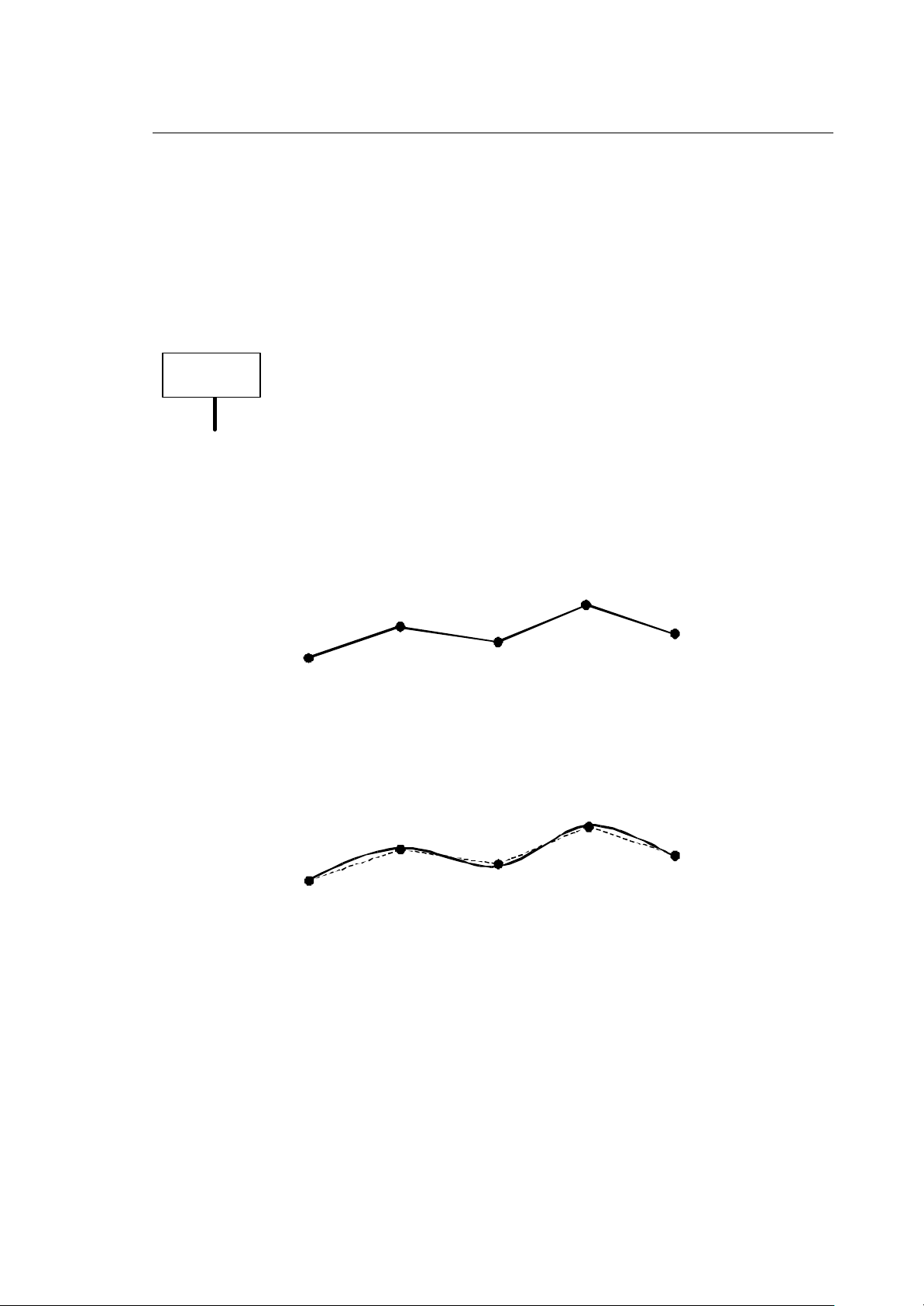
With G01, each point will be linked geometrically to the following ones by means of a polynomial curve, so the generated path may be considered “continuous”. This link will be interrupted by the programming of a G00 or the programming of special G codes described below. The dynamics of the sections in G01 are the same as the “cutting” movements (such as normal G01 movements in ISO programming).

10 Series CNC High Speed Machining (00) 1-3

Chapter 1

G62

High Speed Machining

In addition to the G01 and G00 functions, the following G functions, specific for the HSM feature, may be programmed in the profile.

G61

Determines the start of the profile and must be programmed in a block on its own. When the G61 function is activated, there must be no form of virtualization active (UPR,UVP,UVC,TCP).

Before activating the G61 function, the setup file must be defined by means of the instruction:

(HSM, setup file name)

The G61 command may ONLY be executed within a part program in AUTO or BLK BY BLK status.

G60

Determines the end of the profile and must be programmed in a block on its own. If the machine is in single STEP execution, the profile between G61 and G60 is considered as a

single instruction. To stop its execution, it is necessary to switch to HOLD status.

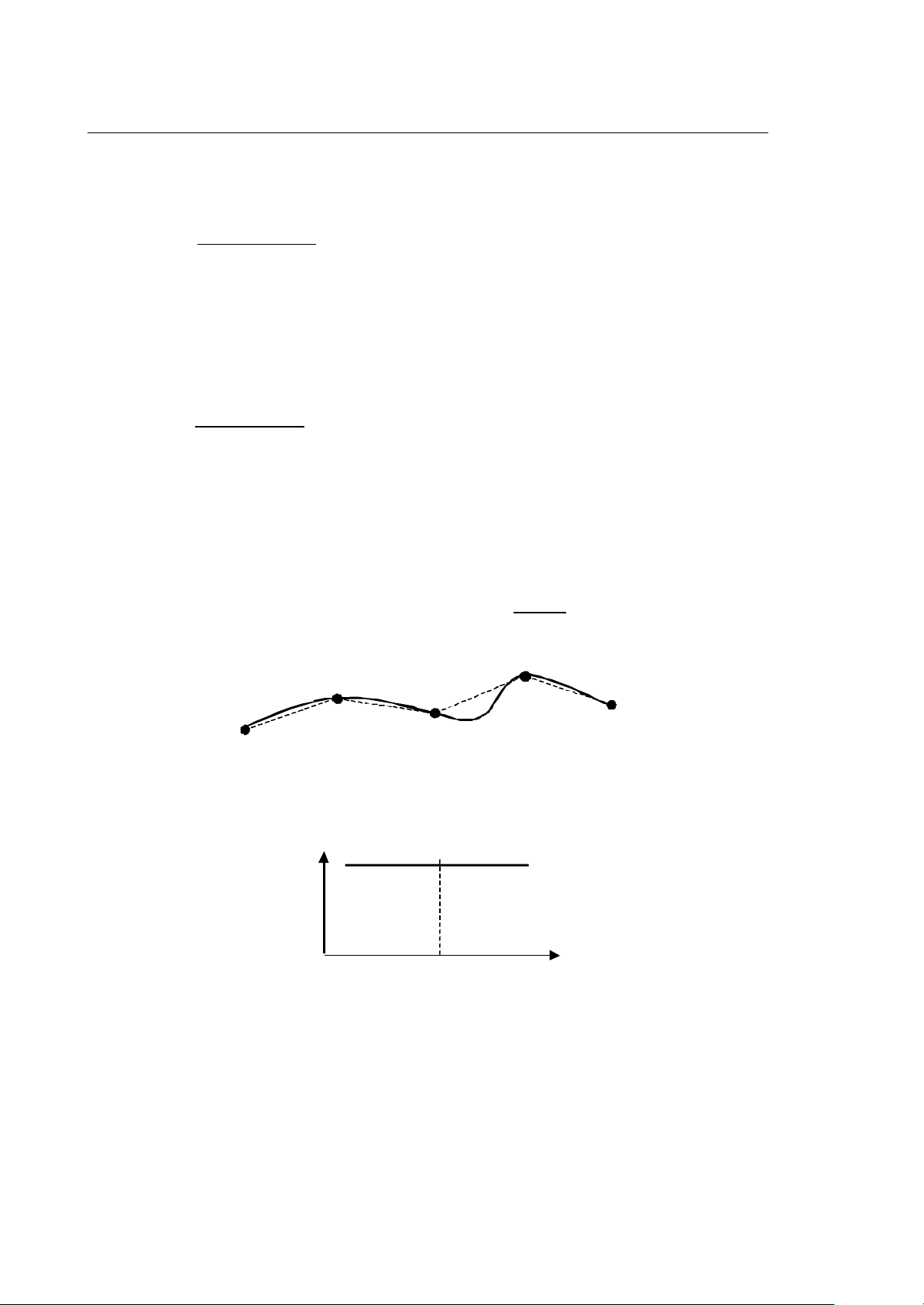
G62

Splits a profile in two parts and determines the point where one profile ends and another begins, maintaining continuity between the two curves.

The points preceding the G62 function will be used to generate a first curve, while the subsequent points will be used to generate another one. These curves will be linked and will therefore be continuous; the initial inclination of the second curve will correspond to the final inclination of the previous curve.

G62

As regards dynamics, with G62 no deceleration and acceleration ramp will be generated to link the two curves. This G function must be programmed in a part program block on its own.

1-4 10 Series CNC High Speed Machining (00)

Chapter 1

High Speed Machining

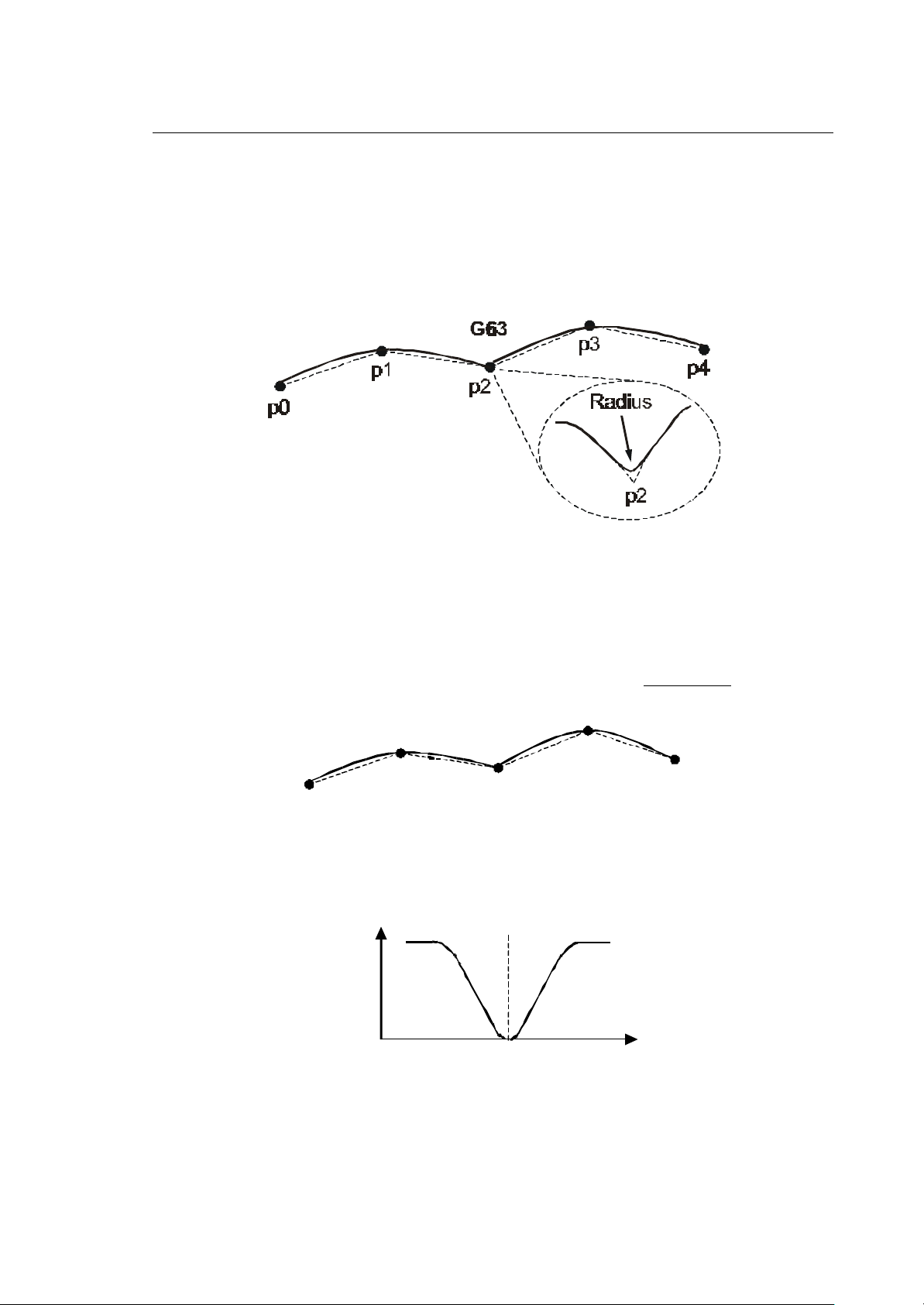
G63

Splits a profile into two parts and determines the point where one profile ends and the other one begins, maintaining continuity between the two curves. The points preceding the G63 function will be used to generate a first curve, while the subsequent points will be used to generate another one. While with G62, the initial inclination of the second curve depends strictly on the final inclination of the first, with G63, the initial inclination of the second curve IS NOT influenced by that of the first. To maintain continuity, a “radius” that depends on the chordal error with which the splines are to be calculated is inserted.

With G63 a reduction in speed may occur at the point where the two curves are linked. This G function must be programmed in a part program block on its own.

G66

Splits a profile into two parts and determines the point where one profile ends and the other one begins, creating a discontinuity between the two curves, that is, the point preceding the G66 represents an edge. At this point, two curves are generated, the first using the points preceding the G66 function and the second using the subsequent points. These curves will NOT be linked, and so there will be a discontinuity.

G66

This discontinuity will be reached at zero speed; the first curve will therefore end with a deceleration ramp to 0 (zero) speed after which the second curve will be tackled with an acceleration ramp to reach the required machining speed. This G function must be programmed in a part program block on its own.

G66

10 Series CNC High Speed Machining (00) 1-5

Chapter 1

High Speed Machining

G67

With G67, a “discontinuity” may be defined on the profile defined with G66. What changes is the dynamic approach to the edge, that is, the end of the curve is not reached at zero speed but at a speed value (vs) that enables the axes to reach the edge without any dynamic problems. This speed value is calculated on the basis of the acceleration that may be withstood by each axis. This G function must be programmed in a part program block on its own.

G67

Considerations on the use of the G62,G63,G66 and G67 functions (transition codes)

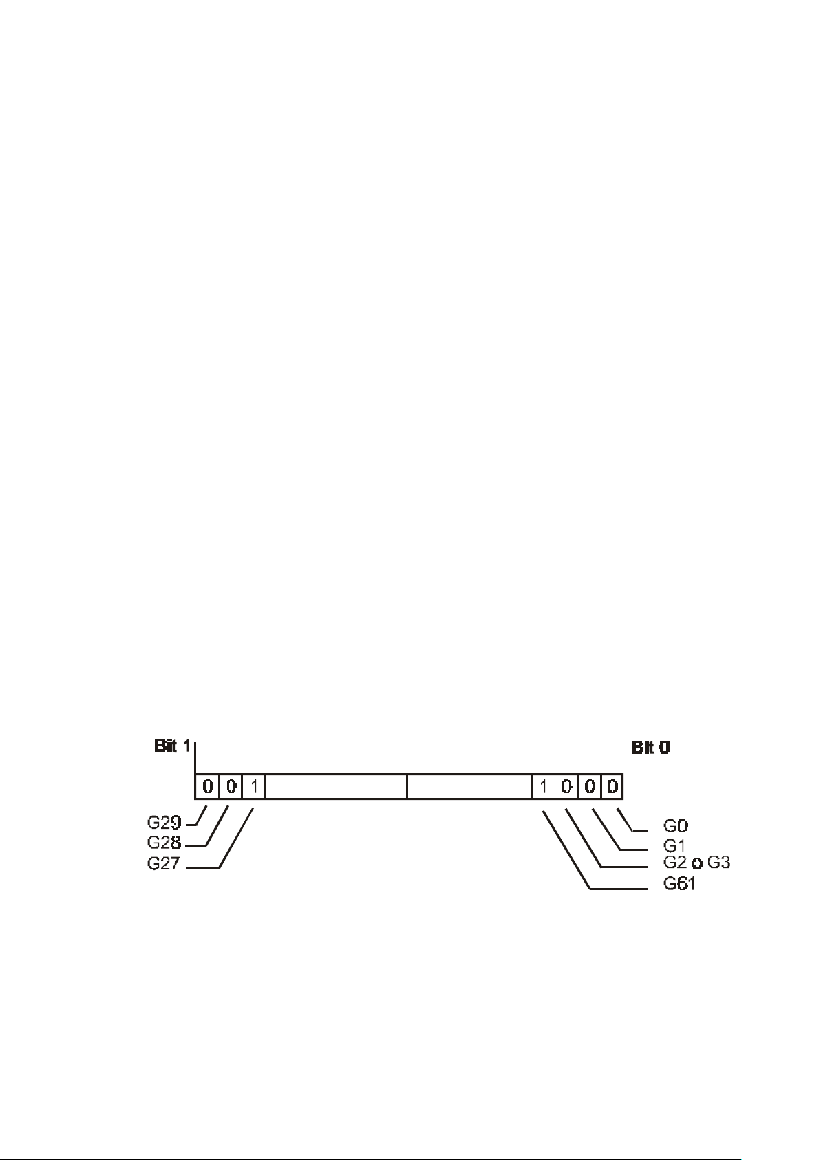
The transition G codes are particularly useful when “similar”, repetitive curves are to be defined (providing the programmed points are also similar and repetitive).

Supposing we have a profile defined by 100 points of which the first 50 represent the first machining pass (from p1 to p50) and the other 50 (from p50 to p99) the same profile shifted slightly (second pass).

p50

As the points between p1 and p50 are “similar” to the points between p50 and p99, the conditions for calculating the two polynomial curves will also be similar. Two “parallel”, almost identical curves will therefore be generated.

If the G62 function has not been programmed on point p50 the NC may generate curves that are not perfectly parallel. This normally undesired effect is due to the fact that the calculation of the polynomial takes into account the “history” along the calculated paths.

The “history” of point p1 is clearly different from that of point p50. In fact, point p1 has no history while in point p50, the NC has followed a path determined by the first 49 points.

p99

When the G62 function is inserted, it cancels the “history” and produces a geometrical pattern almost identical to the one calculated starting from point p1.

In machining processes that entail several passes, failure to program G62 would have the undesirable effect of producing different levels of machining between one pass and another.

1-6 10 Series CNC High Speed Machining (00)

Chapter 1

High Speed Machining

GENERAL HIGH SPEED MACHINING PROGRAMMING STRUCTURE

Between the G61 and G60 blocks it will only be possible to program the points that make up the profile to be machined or the G codes for defining their management method: no other type of programming will be allowed.

Points may be programmed using, absolute programming may be used by means of (G90) or incremental programming by means of (G91). All numerical parameters required may be defined directly or by means of E or L variables: programming with expressions is not valid so XE(E2) or X(E1+E2) type programming is not allowed, while XE1 is allowed.

The syntax of the allowed program lines will be: N… [G00 | G01] [G90 | G91] [points] F…. N… [G62 | G63 | G66 |G67 ] Activation of the HSM (High Speed Machining) feature G61 forces of G01 and G90, modes while at

the exit (G60) the G functions active when G61 was programmed will be restored. The first point programmed MUST be expressed in absolute positions (G90) and must contain the

programming of all axes associated with the HSM programming (axes configured in the HSM setup file).

Interaction with Machine Logic

The G61/G60 program section will be considered, from the system point of view, as a single program block. As regards interfacing with the machine logic, a request for consent for movement will be made when the G61 function is reached, and an end of movement request will be made when the G60 function is reached (in the same way as for the G27 and G28 continuous movements).

A regards consent for movement, the XW03 variable, which contains the type of movement, will be set as shown below:

10 Series CNC High Speed Machining (00) 1-7

Chapter 1

High Speed Machining

END OF CHAPTER

1-8 10 Series CNC High Speed Machining (00)

Chapter

Axis location points

POINT DEFINING CONVENTIONS

POINTS AND MACHINING COORDINATES

Before defining how the points are handled, it is necessary to specify what they represent as programming may be executed in relation to three types of coordinates, that is:

• Cutter Contact Points, which refer to the actual cutting point

• Cutter Location Points, which refer to the point normally indicated as the centre of the tool

• Axis Location Points, which refer to an arbitrary point fixed to the machining axes

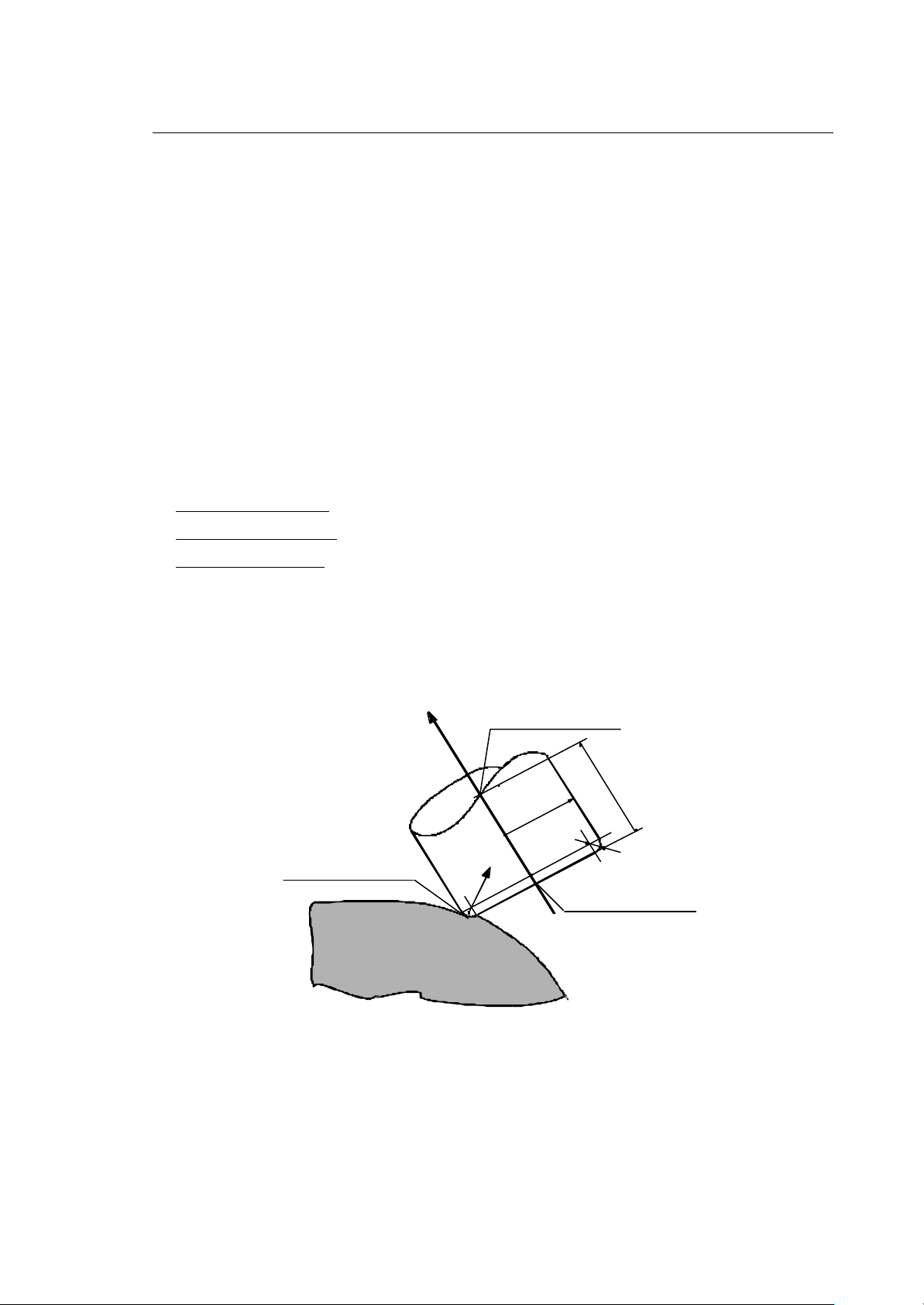
The cutter contact points are linked to the cutter location points through the geometry and orientation of the tool. The axis location points are linked to the cutter location points through the geometry of the machine tool. In machining processes with three axes, the coordinates will simply be translated while, in those with five coordinated axes, rototranslation matrices that take into account the geometrical transformations due to the movement of the rotary axes will be applied. The figure below shows what is meant by cutter contact points, cutter location points and axis location points.

Tool direction

Cutter contact points

Points are defined by means of normal axis coordinates in the format [Axis name][Position]; example: X100 Y200 Z40.

Normal

to surface

Tool

length

Radius

Edge

radius

Cutter location points

10 Series CNC High Speed Machining (00) 2-1

Chapter 2

Point Defining Conventions

Tool Direction

The tool direction represents the orientation of the tool (from the tip to the attachment) within the part reference system.

WARNING

Two methods may be used to define the tool direction. The first is by directly programming the versor that identifies the tool direction. This versor is expressed using the ijk coordinates in the format:

[i] [X-coordinate component] [j][Y-coordinate component] [k][Z-coordinate component] The system will automatically normalize the length of the versor to the unitary length (1.0). The second way of defining the tool direction is by programming the rotary axes. The system will

automatically determine the three components of the ijk versor depending on the kinematics of the machine.

In the following sections reference to versor means versor of unitary lenght.

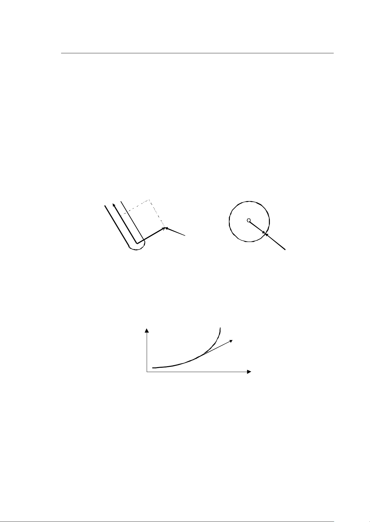
Normal to the Surface Direction

The normal to the surface direction represents the direction of the “line” perpendicular to the surface to be machined (starting from the surface) within the part reference system.

There are two ways of defining the direction normal to the part. The first is by directly programming the versor that identifies the normal direction. This versor (of a unitary length) is expressed using the mno coordinates in the format:

[m] [X-coordinate component] [n][Y-coordinate component] [o][ Z-coordinate component] The system will automatically normalize the length of the versor to the unitary length (1.0). The second way is to have this direction calculated automatically by the system. The direction is

calculated on the basis of the tangent to the profile (direction of the movement), on the basis of the tool direction (ijk versor) and an angle of contact between the part and the tool. This calculation makes sure that the mno versor is normal to the tangent to the profile and that it defines an angle αα (angle of contact) with the tool versor ijk.

ijk

mno

This type of approach is only significant when the contour is to be machined. When a surface is to be machined, this approach could fail as there is no information about the “surface” to be machined, only information about the “direction” of displacement.

tg profile

2-2 10 Series CNC High Speed Machining (00)

Chapter 2

ijk

Point Defining Conventions

Tool Radius Application Direction

The direction of application of the tool radius represents the direction in which radius compensation is to be applied (starting from the centre of the tool) within the part reference system.

There are two ways of defining the tool radius application direction. The first is by directly programming the versor that identifies the direction. This versor (of a unitary length) is expressed using the pqd coordinates in the format

[p] [X-coordinate component] [q][Y-coordinate component] [d][Z-coordinate component]

The system will automatically normalize the length of the versor to the unitary length (1.0). The second way is to have this direction calculated automatically by the system. The direction is

calculated automatically on the basis of the tool direction (ijk versor) and the normal to the part (mno versor). This calculation ensures that the pqd versor is normal to the tool direction and is on the plane formed by the ijk and mno versors.

ijk

pqd

mno

Programming of the versor pqd is only significant when specific cutting strategies are applied.

Tangential Axis

The tangential axis is an axis whose position is calculated so as to remain tangential to the profile described. It is calculated on the basis of the tangent to the polynomial curve on the work plane.

Tangential axis

An initial value of the tangential axis (first programmed point) may be defined and the subsequent positions may be calculated on the basis of this value.

10 Series CNC High Speed Machining (00) 2-3

Chapter 2

Point Defining Conventions

END OF CHAPTER

2-4 10 Series CNC High Speed Machining (00)

Chapter

FEATURES PROVIDED BY HIGH SPEED MACHINING

Depending on the type of machine tool used, the points programmed and a series of additional parameters, the features may be obtained using “High Speed Machining”.

MACHINES WITH 5 AXES

Machines with 5 axes are characterised by the fact that they have two rotary axes that are used to orient the tool during the machining phase. The direction of the tool and the position of the rotary axes are two closely related parameters.

One feature of High Speed Machining is that it “automatically” calculates the position of the rotary axes on the basis of the tool direction (ijk vector). In this way, the same part program may be used on machines having different kinematics providing both machines can reach the same positions.

10 Series CNC High Speed Machining (00) 3-1

Chapter 3

Features Provided by High Speed Machining

Tool Radius and Length Compensation

In order to use tool radius and length compensation, the type of axis positions and vectors as defined in the table below must be included in the part program. The feed rate may refer to the point of contact between the tool and the part (chip removal speed, therefore at the Cutter Contact Point) or the centre of the tool (at the Cutter Location Point). The difference between these two types of settings is significant when tools with a large diameter are used, that is, where the path of the centre of the tool is significantly different from that of the profile of the part.

Setting Description

Axis positions The points must be expressed in Cutter Contact Points Tool Direction The ijk vector or the positions of the rotary axes must be programmed Normal to Surface The mno vector must be programmed or automatically calculated by the

system

Radius Application The pqd vector must be programmed or automatically calculated by the

system

Example:

N001 G61 N002 G1 X10Y10Z10 i0j0k1 m0n0o1 p0q0d1 F10000 N002 X20Y10Z10 ….. N100 G60

Tool Length Compensation

In order to use tool length compensation, the type of axis position and vectors as defined in the table below must be included in the part program. The feed rate will refer to the centre of the tool (at the Cutter Location Point).

Setting Description

Axis Position The points must be expressed in Cutter Location Points Tool Direction The ijk vector or the positions of the rotary axes must be programmed Normal to Surface Ignored Radius Application Ignored

Example:

N001 G61 N002 G1 X10Y10Z10 i0j0k1 F10000 N002 X20Y10Z10 …. ….. N100 G60

3-2 10 Series CNC Hi gh Speed Machining (00)

Chapter 3

Features Provided by High Speed Machining

No Tool Compensation

In this case, only the positions of the axes as defined in the table below have to be included in the part program. The feed rate will refer to the actual movement of the axes (Axis Location Point). The feed rate may however be set is relation to the centre of the tool (Cutter Location Points).

Setting Description

Axis Positions The points must be expressed in Axis Location Points Tool Direction The positions of the rotary axes must only be programmed if the setting of

the feed rate in relation to the tool centre has been requested. If it has not,

the setting is ignored. The ijk vector cannot be programmed. Normal to Surface Ignored Radius Application Ignored

Example:

N001 G61 N002 G1 X10Y10Z10 A10 B10 F10000 N002 X20Y10Z10 …. ….. N100 G60

Tangential Axis Management

If the tangential axis is associated with a rotary axis, its position (calculated by the system) is used to rotate the Tool Direction vector (ijk) so as to keep it tangential to the profile. In this case, the Tool Direction vector must NOT be programmed in the part reference system but in relation to the direction of the movement.

10 Series CNC High Speed Machining (00) 3-3

Chapter 3

Features Provided by High Speed Machining

MACHINES WITH 3 AXES

Generic machines or machines with 3 axes are characterised by the fact that they do not have axes for orienting the tool during the machining phase. The tool direction is generally fixed.

Tool Radius and Length Compensation

Setting Description

Axis positions The points must be expressed in Cutter Contact Points Tool Direction The tool direction vector is defined during the setup phase (on a 3-axis

machine, it is fixed) and remains unchanged throughout the machining process. Programming of the ijk vector is ignored.

Normal to Surface The mno vector must be programmed or automatically calculated by the

system

Radius Application The pqd vector must be programmed or automatically calculated by the

system

Example:

N001 G61 N002 G1 X10Y10Z10 m0n0o1 p0q0d1 F10000 N002 X20Y10Z10 …. ….. N100 G60

3-4 10 Series CNC Hi gh Speed Machining (00)

Chapter 3

Features Provided by High Speed Machining

Tool Length Compensation

Setting Description

Axis Position The points must be expressed in Cutter Location Points Tool Direction The tool direction vector is defined in the setup phase (on a 3-axis machine,

it is fixed) and remains unchanged throughout the machining process.

Programming of the ijk vector is ignored. Normal to Surface Ignored Radius Application Ignored

Example:

N001 G61 N002 G1 X10Y10Z10 F10000 N002 X20Y10Z10 …. ….. N100 G60

No Tool Compensation

In this case, only the positions of the axes as defined in the table below have to be included in the part program. The feed rate will refer to the actual movement of the axes (Axis Location Point). The feed rate may however be set in relation to the centre of the tool (Cutter Location Points).

Setting Description

Axis Positions The points must be expressed in Axis Location Points Tool Direction The tool direction vector is defined during the setup phase (on a 3-axis

machine it is fixed) and remains unchanged throughout the machining

process. It is only used if the setting of the feed rate in relation to the centre

of the tool has been requested, otherwise it is ignored. Programming of the

ijk vector is ignored. Normal Surface Ignored Radius Application Ignored

Example

N001 G61 N002 G1 X10Y10Z10 F10000 N002 X20Y10Z10 …. ….. N100 G60

10 Series CNC High Speed Machining (00) 3-5

Chapter 3

Features Provided by High Speed Machining

Tangential Axis Management

When management of the tangential axis is requested, its position is calculated automatically by the system. Any programming of the tangential axis within the part program defines further rotations of the axis with respect to the tangent calculated by the system. The programming of the value 0 (zero) on the axis activates the calculation of the position by the High Speed algorithms.

END OF CHAPTER

3-6 10 Series CNC Hi gh Speed Machining (00)

Chapter

ADDITIONAL PROGRAMMING MODES

Up to now we have always talked about programming by means of points i.e. the points defined in the part program represent the entities out of which polynomial curves are calculated. But appropriate programming allows direct definition of polynomial curves or to define curves using B-Splines.

POLYNOMIAL PROGRAMMING

A polynomial curve is defined by a function of the type: f(s) = a0 + a1s1 + a2s2 + a3s3 + a4s4 + a5s in which a0 an are the polynomial coefficients

s1 sn are the polynomial parameters which run from 0 to a certain value S (Length of the

polynomial)

The example above defines a polynomial of the 5th degree. On programming level you can also define polynomials of the 3rd and the 4th degree. The degree of a polynomial is defined by associating the parameter P to G61 at High Speed start. For example, in order to program with 3rd degree polynomials you have to write:

G61 P3

In case the P parameter is omitted, the 5th degree is programmed as default. In order to program a polynomial curve you firstly have to define some global parameters of the polynomial and then the polynomial coefficients for all axes configured in the HIGH SPEED set-up. For example, polynomials directly referring to the positions of the X, Y and Z axis are programmed as follows:

<*, Polynomial Length, Block Number, Feed, Transition Code <X, x0 , x1 , x2 , x3 , x4 , x <Y, y0 , y1 , y2 , y3 , y4 , y <Z, z0 , z1 , z2 , z3 , z4 , z

10 Series CNC High Speed Machining (02) 4-1

Chapter 4

Additional Programming Modes

where the line <* defines the global parameter of the polynomial with the following meaning:

PROGRAMMING DESCRIPTION

Polynomial Length defines the upper limit for the parameter s Block Number represents the N of normal ISO programming Feed speed of executing the polynomial Transition code defines how to finish the polynomial and corresponds to the codes

G66 (1) and G67 (2). All other values are ignored. Therefore you cannot program some G codes between one polynomial curve and the next. The only G code admitted is G60 for closing programming.

The line <axis defines the polynomial coefficients.

IMPORTANT

It has to be stressed that the final point of a polynomial (the point defined by fn(S)) MUST be identical to the starting point of the next polynomial (defined by f

n+1

(0)).

4-2 10 Series CNC High Speed Machining (02)

Chapter 4

Additional Programming Modes

POLYNOMIAL PROGRAMMING TYPES AND LIMITS

Based on the type of points defined you also have to program the polynomials for the versors along which to calculate the tool length and the tool radius compensation in addition to the axes polynomials:

Polynomial for the Cutter Contact

<*, Polynomial Length, Block Number, Feed, Transition Code <X, x0 , x1 , x2 , x3 , x4 , x <Y, y0 , y1 , y2 , y3 , y4 , y <Z, z0 , z1 , z2 , z3 , z4 , z <i, i0 , i1 , i2 , i3 , i4 , i <j, j0 , j1 , j2 , j3 , j4 , j <k, k0 , k1 , k2 , k3 , k4 , k <m, m0 , m1 , m2 , m3 , m4 , m <n, n0 , n1 , n2 , n3 , n4 , n <o, o0 , o1 , o2 , o3 , o4 , o <p, p0 , p1 , p2 , p3 , p4 , p <q, q0 , q1 , q2 , q3 , q4 , q <d, d0 , d1 , d2 , d3 , d4 , d

The following considerations apply:

• The parameters "Polynomial Length" and the relative “Feed” have to refer to the

IMPORTANT

curve on the Cutter Contact.

• The polynomials for the three versors (ijk, mno and pqd) MUST always be programmed. Therefore you CANNOT request their automatic calculation or determine their values based on the positions (polynomials) of the rotational axes.

• The automatic calculation of the tangent axis is not managed.

10 Series CNC High Speed Machining (02) 4-3

Chapter 4

Additional Programming Modes

Polynomials for the Cutter Location

The following considerations apply:

• The parameters "Polynomial Length" and the relative “Feed” may refer to any

IMPORTANT

curve (Cutter Contact, Cutter Location, arbitrary), therefore the parameterisation of the polynomial is free.

• The polynomial for the tool direction versor (ijk) MUST always be programmed. Therefore you CANNOT determine their values based on the positions (polynomials) of the rotational axes.

• The automatic calculation of the tangent axis is not managed.

4-4 10 Series CNC High Speed Machining (02)

Polynomials for the Axis Location

<*, Polynomial Length, Block Number, Feed, Transition Code

Chapter 4

Additional Programming Modes

<X, x0 , x1 , x2 , x3 , x4 , x <Y, y0 , y1 , y2 , y3 , y4 , y <Z, z0 , z1 , z2 , z3 , z4 , z

The following considerations apply:

• The parameters "Polynomial Length" and the relative “Feed” may refer to any

IMPORTANT

curve (Cutter Contact, Cutter Location, arbitrary), therefore the parameterisation of the polynomial is free.

• The automatic calculation of the tangent axis is not managed.

For all programming types described above you can also calculate polynomials for additional axes but you have to apply the HSM configuration rules described

WARNING

below.

Example:

G61 P5 <*,4.000000000e+001,3,3000,1 <X,-3.835260000e+002,0.000000000e+000,-4.440892099e-016,1.850371708e-017,-5.782411587e-019,1.355252716e021 <Y,-1.121540000e+002,-1.776356839e-015,1.110223025e-016,4.625929269e-018,7.228014483e020,0.000000000e+000 <Z,2.000000000e+002,-1.000000000e+000,-2.220446049e-016,0.000000000e+000,7.228014483e-020,-6.776263578e022 <i,0.000000000e+000,0.000000000e+000,0.000000000e+000,0.000000000e+000,0.000000000e+000,0.000000000e+000 <j,-5.375997577e-003,-1.084202172e-019,0.000000000e+000,0.000000000e+000,-8.823259867e-024,6.893171771e027 <k,9.999855492e-001,1.387778781e-017,-8.673617380e-019,0.000000000e+000,-1.411721579e-021,-1.764651973e024 <*,2.488900000e+001,5,3000,5 <X,-3.835260000e+002,0.000000000e+000,-8.881784197e-016,7.401486831e-017,0.000000000e+000,-1.445602897e020 <Y,-1.121540000e+002,-3.552713679e-015,0.000000000e+000,9.251858539e-018,0.000000000e+000,1.807003621e021 <Z,1.600000000e+002,-1.000000000e+000,0.000000000e+000,-3.700743415e-017,-2.023844055e-018,1.626303259e020 <i,0.000000000e+000,0.000000000e+000,0.000000000e+000,0.000000000e+000,0.000000000e+000,0.000000000e+000 <j,-5.375997577e-003,-2.168404345e-019,1.355252716e-020,0.000000000e+000,6.176281907e-023,2.205814967e-025 <k,9.999855492e-001,0.000000000e+000,0.000000000e+000,0.000000000e+000,-6.776263578e-021,2.823443158e-023 <*,6.557923113e+001,64,3000,5 <X,-3.836260000e+002,-8.775202787e-013,8.304468224e-014,-2.544261098e-015,3.13695828e-017,-1.359876104e019

10 Series CNC High Speed Machining (02) 4-5

Chapter 4

Additional Programming Modes

<Y,-1.736380000e+002,4.116045842e-001,3.370526100e-003,1.039559753e-005,1.237013981e-007,-1.997131743e009 <Z,8.603200000e+001,9.164030615e-001,-2.215163382e-003,1.562230248e-005,-6.930401526e-007,3.106008361e009 <i,0.000000000e+000,0.000000000e+000,0.000000000e+000,0.000000000e+000,0.000000000e+000,0.000000000e+000 <j,-9.155922041e-001,5.944508142e-003,-1.757065214e-004,6.214612678e-006,-5.203550510e-008,1.330231937e-010 <k,4.021080896e-001,6.332656007e-003,9.717969494e-005,-8.784047262e-007,-5.093874428e-009,3.500516597e-011 G60

4-6 10 Series CNC High Speed Machining (02)

Chapter 4

Additional Programming Modes

B-SPLINES PROGRAMMING

Programming with B-Splines is similar to programming by means of points. The only difference is that the programmed points are NOT points through which the curve runs: they are the "curve control points". In this sense the curve tries to pass as smoothly as possible between the programmed points. If you are not familiar with B-Splines, you should study their theory in order to understand their

programming and the terminology used.

A B-Spline curve is defined as:

P(s) = Σ P

i=1

i Ni,d

(s)

where s B-Spline parameter

n number of control points P(s) the point calculated for the parameter s P

i,d

ith control point dth B-Spline base function value

The formula defined above defines a B-Spline curve of the nth degree. You can program B-Spline curves of the 3rd, 4th and 5th degree. The degree of the programmed B-Splines is defined by associating the parameter P to G61 at High Speed start. For example, in order to program with 3rd degree B-Splines you have to write:

G61 P3

In case the P parameter is omitted, the 5th degree is programmed as default. In order to program a B-Spline curve you have to define the control points for all axes configured in the HIGH SPEED set-up as well as the elements of the knot vector. For example, B-Splines directly referring to the positions of the X, Y and Z axis are programmed as follows:

N100 X… Y… Z.. K.. F.. where X Y and Z define the control points

N defines the Block Number F defines the Feed K defines the knot. The number of knots has to be equal to the number of control

points plus the B-Spline degree plus 1. So for a 5th B-Spline operating on 10 point you have to define 16 knots. In addition the first n+1 and the last n+1 values (n being the B-Spline degree) HAVE to have the same value and all values must be expressed in incremental order. You can re-initialise the knot vector after each G.

You can program G62, G66 and G67 between one B-Spline and the next. The

IMPORTANT

final control point of a B-Spline must coincide with the first one of the following BSpline.

10 Series CNC High Speed Machining (02) 4-7

Chapter 4

Additional Programming Modes

B-SPLINE PROGRAMMING TYPES AND LIMITS

Based on the type of points defined you also have to program the B-Splines for the versors along which to calculate the tool length and the tool radius compensation in addition to the axes B-Splines:

B-Splines for Cutter Contact

N100 X… Y… Z.. i… j… k… m… n… o.. p.. q... d.. K.. F… The following considerations apply:

• The parameters K and the relative “Feed” have to refer to the curve on the Cutter Contact.

• The control points for the three versors (ijk, mno and pqd) MUST always be programmed.

Therefore you CANNOT request their automatic calculation or determine their values based on the positions (B-Splines) of the rotational axes.

• The automatic calculation of the tangent axis is not managed.

B-Splines for Cutter Location

N100 X… Y… Z… i.. j.. k.. K.. F… The following considerations apply:

• The parameters K and the relative “Feed” may refer to any curve (Cutter Contact, Cutter Location, arbitrary), therefore the parameterisation of the B-Spline is free.

• The control points for the tool direction versor (ijk) MUST always be programmed. Therefore you CANNOT determine their values based on the positions (B-Splines) of the rotational axes.

• The automatic calculation of the tangent axis is not managed.

B-Splines for Axis Location

N100 X… Y… Z… K.. F… The following considerations apply:

• The parameters K and the relative “Feed” may refer to any curve (Cutter Contact, Cutter Location, arbitrary), therefore the parameterisation of the B-Spline is free.

• The automatic calculation of the tangent axis is not managed.

4-8 10 Series CNC High Speed Machining (02)

WARNING

Example:

G61 P3 X0 Y0 Z0 K0 F3000 X0.7 Y2.3 Z0 K0 X3.8 Y2.6 Z0 K0 X2.3 Y-1.5 Z0 K0 X6.9 Y-1.5 Z0 K2.5 X6.1 Y1.2 Z0 K5 X8.4 Y1.5 Z0 K7.5 K10. K10 K10 K10 G60

Chapter 4

Additional Programming Modes

For all programming types described above you can also calculate B-Splines for additional axes but you have to apply the HSM configuration rules described below.

10 Series CNC High Speed Machining (02) 4-9

Chapter 4

Additional Programming Modes

END OF CHAPTER

4-10 10 Series CNC High Speed Machining (02)

SETUP

A special file (part program) contains the setup of the HSM environment. This setup is activated whenever the G61 code is programmed. All numerical values may be defined directly or by means of E or L parameters.

The setup file may be divided into three sections:

− a section of General three-letter codes

− a section of Axis Setup three-letter codes

Chapter

− a section of Machine Setup three-letter codes, which define the kinematics of the machine. General Three-Letter Codes

(PNT,Type,Param,Poly,Format) Definition of types of points (VER,Ijk,Mno,Pqd) Versor management (JRK,Mode,Jrs,Entities,Tstab,Tintgr,Ttop) Look Ahead management (THR,Tol,TolV,Scale,NullMov,Chord) Threshold programming (TOL,Len,Radius,EdgeRad,Angle,OriginLen) Tool definition (TOD,Xcomp,Ycomp,Zcomp) Tool direction (3D) (CRV,Len,Ratio,Mode) Change in curvature management (EDG,Angle,VAngle,Mode,Acc) Edge management

Axis Setup Three-Letter Codes

(AXI,Name,Id,Type,CinType,Diam) Definition of types of axis (AXP,Name,NullMov,Pitch,Lim-,Lim+) Definition of axis parameters (DIN,Name,Vmax,Amax,Jmax,Vrap,Arap,Jrap) Definition of axis dynamics

Machine Setup Three-Letter Codes

(MAC,Type,Bed) Definition of type of machine (CIN,Name,Xoff,Yoff,Zoff,Xrot,Yrot,Zrot) Definition of machine kinemat ics

Path Optimizer configuration Three-Letter Codes

(SMT,Toll,TollV,Racc,RaccV,C0,C0V) Tolerances and smoothing parameters (SMS,Split,SplitV,CondI,CondU,Len,Pnt,C1,Dbg) Special smoothing parameters

10 Series CNC High Speed Machining (02) 5-1

Chapter 5

Setup

TYPE OF POINTS DESCRIBED IN THE PART PROGRAM

The syntax of the three-letter code that defines the type of points described in the part program is as follows:

(PNT, Type, Param, Poly, Format) example: (PNT, CLP,CLP,QUI,PNT)

Parameter Type Values Description

Type Character CCP

CLP AXI Obligatory

Param Character CCP

CLP AXI Obligatory

Defines the type of points described in the Part Program CCP Cutter Contact Points: the points entered are

defined in “Cutter contact points”, so tool compensation (radius and length) may be executed on these points.

CLP Cutter Location Points: the points entered are

defined in “Cutter location points“, so tool compensation (length only) may be executed on these points.

AXI Axis Location Points: the points entered are

defined in “Axis location points”, so no type of compensation may be executed on these points.

Defines the type of profile for which the feed rate is programmed in the Part Program and depends on the type of points entered. The feed rate always refers to the “3D” profile. Any rotary or additional axes present are not involved in the calculation of the feed rate but “follow” the execution of the 3D profile. The feed rate is however limited when the latter axes, in following the 3D axes, tend to exceed their dynamic limits.

CCP The programmed Feed rate refers to the profile

generated on the “Cutter contact points”; this setting is clearly only valid if the points entered are of the CCP type.

CLP The programmed Feed rate refers to the profile

generated on the “Cutter location points”; it may be used for the CCP and CLP type points, while for AXI type points it is only valid when the tool direction can be determined (either from the programming of the rotary axes or from the programming of the ijk versors).

AXI The programmed Feed rate refers to the profile

generated on the “Axis location points”; it may only be used for AXI type points.

Poly Car. CUB or QUI

Obligatory

Format Characters PNT, POL or

BSP optional

5-2 10 Series CNC High Speed Machining (02)

Defines the degree of the polynomial curve generated for the execution of the programmed profile.

CUB A cubic polynomial is generated. QUI A quintic polynomial is generated.

defines the profile programming method i.e. the input format used.

PNT input in point format POL input in polynomial format BSP input in B-Spline format

Chapter 5

Setup

VERSOR MANAGEMENT METHODS

The syntax of the three-letter code that defines how to manage the versors is as follows:

(VER, Ijk, Mno, Pqd) example: (VER , REL , PRG , PRG )

Parameter Type Values Description

Ijk Character PRG or REL

Obligatory

Mno Character PRG or REL

Obligatory

Pqd Character PRG or REL

Obligatory

Defines whether the “Tool Direction” vector is programmed directly by means of the ijk components or whether it is to be calculated on the basis of the position of the rotary axes. When the versor is not necessary, this setting is ignored.

PRG The versor is programmed using the ijk

components.

REL The versor is to be determined from the position of

the rotary axes.

Defines whether the “Normal to Surface” vector is programmed directly using the mno components or whether it is to be calculated automatically by the system. If the versor is not necessary, this setting is ignored.

PRG The versor is programmed using the mno

components.

REL The versor is to be determined automatically by

the system.

Defines whether the “Tool Radius Application Direction” vector is programmed directly using the pqd components or whether it is to be calculated automatically by the system. When the versor is not necessary, this setting is ignored.

PRG The versor is programmed using the pqd

components.

REL The versor is to be determined automatically by the

system.

10 Series CNC High Speed Machining (02) 5-3

Chapter 5

Setup

LOOK AHEAD MANAGEMENT

The syntax of the three-letter code that defines the method of look ahead and dynamics management is as follows:

(JRK, Mode, Jrs, Entities, Tstab, Tintgr, Ttop) example: (JRK, ENA,, )

Parameter Type Values Description

Mode Character ENA,DIS or

AXI Obligatory

Jrs Number Taken from

JRS variable Optional

Entities Number Optional The High Speed algorithm works with a dynamic code

Tstab Number Optional Defines the time window (in ms) within which the speed

Defines the type of dynamics to be used. ENA Enables the use of Jerk Limitation (Mov=8). The

specified jerk refers to the dynamics described on the profile.

DIS Disables Jerk Limitation, only uses “S ramps”

(Mov=2).

AXI Enables the use of Jerk Limitation (Mov=8). The

specified jerk refers to the dynamics described by the axes and how this affects the dynamics of the profile. The use of this method is closely associated with the quality of the points entered (number of decimals and distribution).

Modifies the value of the JRS variable of the system only for the G61 section being processed; if the value is omitted, the JRS variable active in the system is used.

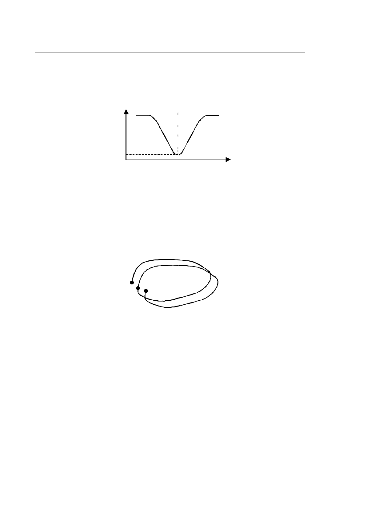
(polynomial curves) and only after having calculated and having filled in the whole queue from the start to the movement.The start may be adjusted by programming the number of elements to be calculated before starting movement. 0 means maximum number of elements.

smoothing algorithm is to be applied. This algorithm removes unnecessary accelerations so as to avoid machine oscillations (see Figure 1).

Tintgr Number Optional Defines the maximum time (in ms) for integrating the

acceleration (or deceleration) phases with the sections at a constant feed rate (see Figure 1).

Ttop Number Optional Defines the minimum time (in ms) for executing a section

with a constant feed rate V (see Figure 1).

5-4 10 Series CNC High Speed Machining (02)

Chapter 5

Setup

Figure 1

10 Series CNC High Speed Machining (02) 5-5

Chapter 5

refers to entities like versors which always have a

Setup

THRESHOLDS

The syntax of the three-letter code that defines the value of thresholds used in generating the polynomial curves is as follows:

(THR, Tol, TolV, Scale, NullMov, Chord) example: (THR , 0.01 , 0.0001 , 0 , 0 , 0.1 )

Parameter Type Values Description

Tol Number Obligatory Defines the tolerance range to be used in generating the

polynomial curves. As defined previously, the polynomial curves generated pass through the programmed points, within a given tolerance threshold. This parameter defines the tolerance value. It is defined in mm (or inches if the machine is configured in inches).

TolV Number Obligatory Defines the tolerance range to be used in generating the

polynomial curves calculated on the versors. This value is important because the precision with which the rotary axes are positioned depends on the precision with which the curves are generated on the versors (in particular, on the ijk versor). The number has no dimension in that it

dimension of 1. We suggest a value equal to 0.1 times the Toll value defined previously be set. 0 disables the management of a tolerance on the versors.

Scale Number Obligatory Scale factor to be applied to the programmed axes. If 0 is

set, the scale factor is not to be applied. It is not applied to the versors and rotary axes, when programmed.

NullMov Number Obligatory Null movement threshold. If the distance between one

point and the next is less than this threshold in mm (or inches if the machine is configured in inches) the next point is eliminated.

Chord Number Obligatory Maximum allowed chordal error at input and output during

the generation of a polynomial. Value expressed in mm (or inches if the machine is configured in inches).

5-6 10 Series CNC High Speed Machining (02)

Chapter 5

Setup

TOOL DEFINITION

In the High Speed Machining system, “Cylindrical”, “Ball-ended” and “Toroidal” type tools may be managed. The syntax of the three-letter code that defines the characteristics of the tool to be used for machining is as follows:

(TOL, Len, Radius, EdgeRad, Angle, OriginLen) example: (TOL , , , 1 , -90 , 0 )

Parameter Type Values Description

Len Number Taken from the

offset active on G61

Optional

Radius Number Taken from the

offset active on G61

Optional

EdgeRad Number Obligatory Defines the radius on the edge of the tool. As this value is

Angle Number Obligatory Defines the angle of contact between the tool and the

OriginLen Number Obligatory Defines the length of the tool for which the part program

Defines the length of the tool to be used for tool length compensation. If no value is set, the tool length is taken from the offsets active in the system on the activation of the G61. The value set here is only active during the machining of the current section of G61/G60.

Defines the radius of the tool to be used for tool radius compensation. If no value is set, the tool radius is taken from the offsets active in the system on the activation of G61. The value set here is only active during the machining of the current section of G61/G60.

not handled by the system offsets, it has to be set.

part. It is used in the automatic calculation of the vector normal to the surface.

was generated. This field is used when the points entered refer to “Axis location points” and the feed rate is to be set in relation to the “Cutter location points”.

10 Series CNC High Speed Machining (02) 5-7

Chapter 5

Setup

TOOL DIRECTION (3D)

Defines the tool direction (to be used for compensation purposes) for generic machines or machines with 3 axes (it is not required on machines with 5 axes). In practice, the unitary vector (similar to ijk) which identifies the tool direction in the part reference system has to be defined. The syntax of the three-letter code that defines the direction of the tool to be used for machining is as follows:

(TOD, Xcomp, Ycomp, Zcomp) example: (TOD , 0 , 0 , 1 )

Parameter Type Values Description

Xcomp Number Obligatory Component of the tool direction along the X axis. Ycomp Number Obligatory Component of the tool direction along the Y axis. Zcomp Number Obligatory Component of the tool direction along the Z axis.

5-8 10 Series CNC High Speed Machining (02)

Chapter 5

Setup

CHANGE IN CURVATURE MANAGEMENT

The algorithm used by the CAM systems to generate the points of a profile takes into account the “chordal error”, that is, it generates points closer together when the radius of curvature of the profile to be described becomes more accentuated. A change in curvature may therefore be generically identified by a variation in the distance between one set of points and the following ones. This variation in curvature may be identified automatically by the High Speed Machining algorithms so as to avoid oscillations around the point where this change takes place.

Supposing, for example, we have a curved section followed by a straight section. The spline on the straight section would tend to oscillate or generate a “hump”, so it is important to identify it.

At the point of the “change in curvature” the system will automatically insert a G62 or a G63 as requested by the user.

The syntax of the three-letter code that defines how to identify and then manage the change in curvature is as follows:

(CRV, Len, Ratio, Mode) example: ( CRV , 1 , 6 , G63 )

Parameter Type Values Description

Len Number Obligatory Defines the minimum length of the “long section” for the

change in curvature to be managed. It is defined in mm (or inches if the machine is configured in inches).

Ratio Number Obligatory Defines the ratio between the long section and short

section so that the change in curvature may be identified. For example, the value 6 defines that the distance between p2 and p3 must be greater than 6 times the distance between p1 and p2 for the change in curvature to be activated.

Mode Character G62 or G63

Obligatory

Defines the transition code to be set on the “change in curvature” point

G62 The two segments are generated with two splines

tangential to one another, so the second spline will have an initial inclination equal to the final inclination of the first spline.

G63 The two segments are generated by two non-

tangential splines, but are linked on the basis of the calculation tolerance set.

10 Series CNC High Speed Machining (02) 5-9

Chapter 5

Setup

EDGE MANAGEMENT

The automatic identification of edges is important for the same reason as the identification of changes in curvature. Failure to identify edges could generated incorrect oscillations on the splines. The optimum dynamic approach for handling an edge is to stop at zero speed and then restart on the next section. Stopping may be damaging however as the tool, as it turns, continues to remove material and so some “notches” may be visible on the part. For this reason, it is possible to define whether and how to stop at the edge.

The syntax of the three-letter code that defines how to identify and therefore how to manage the presence of edges is as follows:

(EDG, Angle, VAngle, Mode, Acc) example: ( EDG , 30 , 0 , G66 , 1 )

Parameter Type Values Description

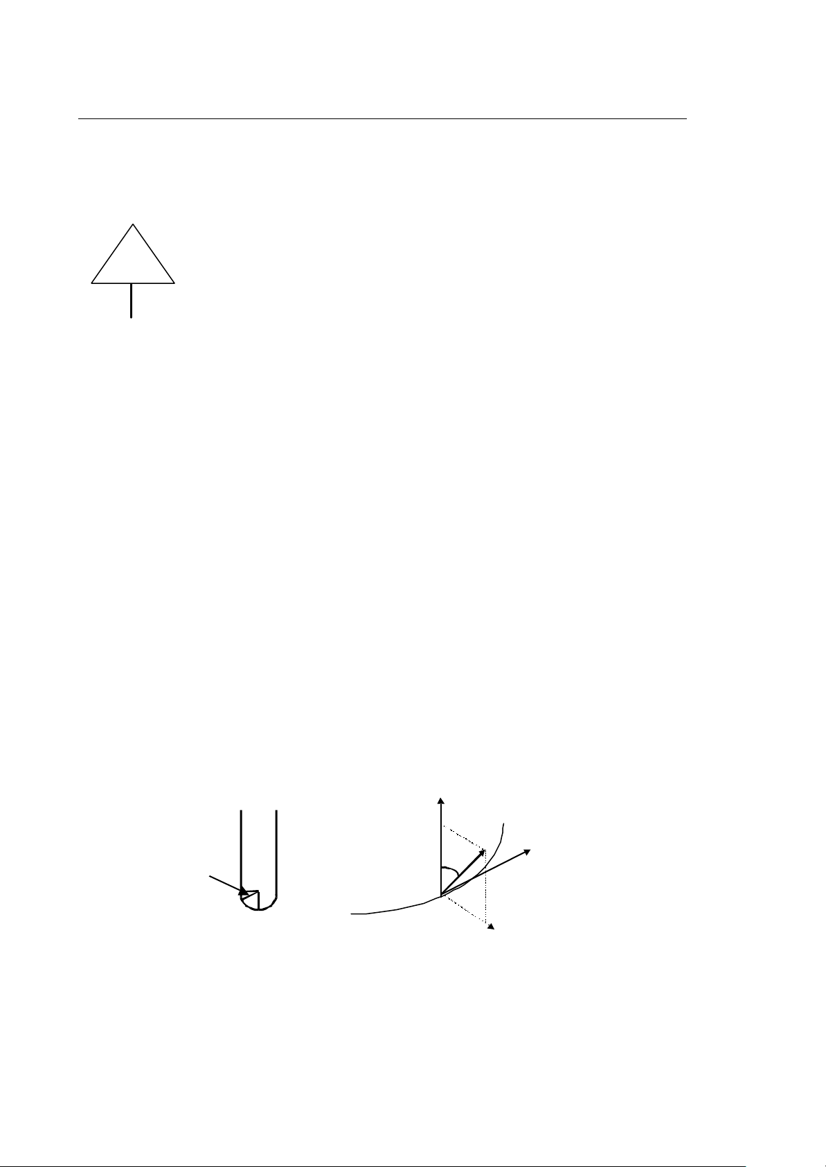
Angle Number Obligatory The system is capable of automatically determining the

edges defined by the programmed points (edges on the linear axes) and automatically programming a G66. This value, expressed in degrees, defines the threshold angle beyond which a point is defined an “edge” point. See the figure below.

VAngle Number Obligatory It is similar to the previous value and is to be used for the

versors. The presence of an edge on the versors generates an “edge” in the movement of the rotary axes. It is therefore advisable to add a G66 also in these cases. See the figure below.

Mode Character G63, G66 or

G67 Obligatory

Acc Number Obligatory Acceleration that may be withstood by the axes in

Defines the transition code to be set on the edge G63 The edge is executed by inserting a link which is

generated by taking the configured chordal error into account.

G66 Movement ends at zero speed. G67 Movement ends at the maximum speed at which

the edge may be faced in the best possible way.

tackling the edge: 1 means that an axis may withstand an increase in speed equal to 1 acceleration. It only applies to G67.

5-10 10 Series CNC High Speed Machining (02)

Chapter 5

Setup

AXIS DEFINITION

The axes to be subjected to the High Speed Machining algorithms may be defined. A maximum of 6 axes may be defined, of which 3 axes make up the three Cartesian axes, 2 are rotary axes (for machines with 5 axes) and other additional axes. The syntax of the three-letter code for defining the axes is as follows:

(AXI, Name, Id, Type , CinType, Diam) example: (AXI , X , 1 , ABS , LI1, DIS)

Parameter Type Values Description

Name Character Obligatory Defines the name of the axis. This name may be different

from the one set in AMP for the axis, and may therefore be compared to an implicit “DIN” in the HSM setup. This association only applies to the G61/G60 section being machined.

Id Number Obligatory Defines the ID of the axis. This axis must be under the

control of the Process in which the part program is being executed.

Type Character ABS, ORD,

VRT, TAN, OTH or TAO

Obligatory

Defines the axis type, and influences the method by which the axis is managed by the HSM algorithms.

ABS The axis is of the x-coordinate type (in the

Cartesian coordinate system)

ORD The axis is of the y-coordinate type (in the

Cartesian coordinate system)

VRT The axis is of the z-coordinate type (in the

Cartesian coordinate system)

TAN Tangential axis, calculated automatically by the

system

TAO tangent axis, automatically calculated by the

system with the moving axis (positive direction) in clockwise sense, i.e. in the sense opposite to the trigonometric convention.

OTH Other type of axis, different from the previous ones.

10 Series CNC High Speed Machining (02) 5-11

Chapter 5

Setup

Parameter Type Values Description

CinType Character LI1, LI2, LI3,

WRK, TOL or OTH

Obligatory

Diam Character ENA or DIS

optional

Defines the position of the axis in the kinematic chain of the machine (see following sections). For generic machines or machines with 3 axes for which the kinematic chain does not have to be defined, we recommend the following setup:

LI1 To be associated with the axis defined as ABS (x-

coordinate) in the previous field.

LI2 To be associated with the axis defined as ORD (y-

coordinate) in the previous field.

LI3 To be associated with the axis defined as VRT (z-

coordinate) in the previous field. OTH Additional axis. For machines with 5 axes, the setup values are as

follows:

LI1 First axis in the kinematic chain. LI2 Second axis in the kinematic chain. LI3 Third axis in the kinematic chain. WRK Rotary axis closest to the part. TOL Rotary axis closest to the tool. OTH Additional axis.

Allows to characterise the axis as Diametral. If not defined, the analog active system parameter is used.

ENA the axis is defined as diametral. DIS normal axis

5-12 10 Series CNC High Speed Machining (02)

Chapter 5

Setup

AXIS PARAMETERS

Some characteristics of the axis set on the system may be varied. These variations are only active in the G61/G60 section being machined. The syntax of the three-letter code is as follows:

(AXP, Name, NullMov, Pitch, Lim-, Lim+) example: (AXP , X , 0 , , , )

Parameter Type Values Description

Name Character Obligatory Axis name as defined in the three-letter code (AXI). NullMov Number Obligatory Defines the null movement for the axis in question. If the

position programmed for an axis differs from the current position (or last programmed position) for a value lower than the null movement, the movement of the axis (the new position) is not considered. We recommend it be left set to 0 and activated only in cases in which the part program under execution contains imprecisions in the programming of the axes.

Pitch Number Optional Used for redefining the rollover pitch for the axis in

question. It may be used, for example, to program a nonrollover rotary axis with rollover values and vice versa. If not defined, the analog active system parameter is used.

Lim- Number Optional Used for redefining the lower operating limit for the axis in

question. If not defined, the analog active system parameter is used.

Lim+ Number Optional Used for redefining the upper operating limit for the axis in

question. If not defined, the analog active system parameter is used.

10 Series CNC High Speed Machining (02) 5-13

Chapter 5

Setup

AXIS DYNAMICS

Some dynamic characteristics of the axis set in the system may be varied. These variations are only active in the G61/G60 section being machined. The syntax of the three-letter code is as follows:

(DIN,Name, Vmax, Amax, Jmax, Vrap, Arap, Jrap) example: (DIN , X , , , , , , )

Parameter Type Values Description

Name Character Obligatory Axis name as defined in the three-letter code (AXI). Vmax Number Optional Used for redefining the maximum speed at which the axis

may be moved when a machining operation in G01 is in progress. It must be defined in mm/min. If not defined, the analog active system parameter is used.

Amax Number Optional Used for redefining the maximum acceleration at which

the axis may be moved when a machining operation in G01 is in progress. It must be defined in mm/sec2. If not defined, the analog active system parameter is used.

Jmax Number Optional Used for redefining the maximum Jerk to which the axis

may be moved when a machining operation in G01 is in progress. It must be defined in mm/sec3. If not defined, the analog active system parameter is used.

Vrap Number Optional Used for redefining the maximum speed at which the axis

may be moved when a machining operation in G00 is in progress. It must be defined in mm/min. If not defined, the analog active system parameter is used.

Arap Number Optional Used for redefining the maximum acceleration at which

the axis may be moved when a machining operation in G00 is in progress. It must be defined in mm/sec2. If not defined, the analog active system parameter is used.

Jrap Number Optional Used for redefining the maximum Jerk at which the axis

may be moved when a machining operation in G00 is in progress. It must be defined in mm/sec3. If not defined, the analog active system parameter is used.

5-14 10 Series CNC High Speed Machining (02)

Chapter 5

Setup

MACHINE KINEMATICS

By configuring the machine kinematics, the various transformations that enable the machine to switch from programming in “Cutter contact points” or “Cutter location points” to the actual movement of the axes may be configured, programming the rotary axes automatically and carrying out the compensation described previously for machines with 5 axes.

Definition of the Kinematic Chain

A fundamental operation in defining the machine kinematics is to identify the “Kinematic Chain” that is, to define the sequence of movements of the axes and define how movement passes from one axis to another. This chain must start from the tool and end at the part.

The kinematics managed by High Speed Machining include 2 rotary axes and 3 linear axes with the possibility of handling the rotary axes in three different layouts:

a) Two rotary axes associated with two rotary tables on which the part to be machined is positioned.

In this case, the kinematic chain is defined as follows : Tool →→ Linear axes →→ First table →→ Second table →→ Part

b) A rotary axis associated with a rotary table on which the part to be machined is positioned and

another rotary axis assembled on the head. In this case, the kinematic chain is defined as follows: Tool →→ Head rotary axis →→ Linear axes →→ Rotary table →→ Part

c) Two rotary axes both assembled on the head (Double twist) that move around the part. In this

case, the kinematic chain is defined as follows :

Tool →→ First head rotary axis →→ Second head rotary axis →→ Linear axes →→ Part

This structure may be illustrated (using the symbols defined in the setup of the three-letter code AXI for the TipoCin) field in the form of the table below:

Tool Rotary Rotary Linear 3 Linear 2 Linear 1 Rotary Rotary Part

T --- --- LI3 LI2 LI1 TOL WRK P T --- TOL LI3 LI2 LI1 WRK --- P T TOL WRK LI3 LI2 LI1 --- --- P

Another fundamental element in the kinematic chain is the “Machine Bed”. It is a “theoretical” point fixed to the ground with respect to which the sequence of movement of the axes (chain) may be split into two sections. The movements of the first section do not influence the movements of the second section.

10 Series CNC High Speed Machining (02) 5-15

Chapter 5

Setup

In the kinematic chain, the “Machine Bed” may have one of four positions, which may be illustrated by means of the table below:

Tool Rotary Rotary Linear 3 Linear 2 Linear 1 Rotary Rotary Part

T --- --- LI3 LI2 LI1 TOL WRK P T --- TOL LI3 LI2 LI1 WRK --- P T TOL WRK LI3 LI2 LI1 --- --- P

Machine Bed

Toll

Machine Bed

B23

Machine Bed

B12

Machine Bed

WRK

The machine kinematics can be extended so that rotational axes (always and only 2) can also be positioned on top of the linear ones. Hence you can describe machines using those cinematic solutions defined as “auxillary axes parallel to the main E axis”. The additional possible cinematic chains are:

a) a rotational axis for a turntable for mounting the piece to be machined and an auxillary axis

parallel to the main E axis for the second linear axis. In this case the cinematic chain is defined as follows:

Tool -> linear axes (3rd and 2nd) -> rotational -> linear axis (1st) -> turntable -> work piece

b) a rotational axis for a turntable for mounting the piece to be machined and an auxillary axis

parallel to the main E axis” for the third linear axis. In this case the cinematic chain is defined as follows:

Tool -> linear axis (3rd) -> rotational -> linear axis (2nd and 1st) -> turntable -> work piece

c) a rotational axis mounted on the head moving around the work piece and an auxillary axis parallel

to the main E axis for the second linear axis. In this case the cinematic chain is defined as follows:

Tool -> rotating head ->linear axes (3rd and 2nd) -> rotational -> linear axis (1st) ->work piece

d) a rotational axis mounted on the head moving around the work piece and an auxillary axis parallel

to the main E axis for the third linear axis. In this case the cinematic chain is defined as follows:

Tool -> rotating head ->linear axis (3rd) -> rotational -> linear axes (2nd and 1st) ->work piece

e) a last configuration with two auxillary axes parallel to the main E axis. In this case the cinematic

chain is defined as follows:

Tool -> rotational ->linear axis (3rd) -> rotational -> linear axis (2nd) -> rotational -> linear axis (1s) ->work piece

5-16 10 Series CNC High Speed Machining (02)

Chapter 5

Setup

This structure can be summarised (using the symbols defined in the configuration of the triletteral AXI for the field TipoCin) with the following table

Tool Rotary Rotary Linear3 Rotary Linear Rotary Linear1 Rotary Rotary Work

piece

T --- --- LI3 --- LI2 TOL LI1 WRK --- P T --- --- LI3 TOL LI2 --- LI1 WRK --- P T --- TOL LI3 --- LI2 WRK LI1 --- --- P T --- TOL LI3 WRK LI2 --- LI1 --- --- P T --- --- LI3 TOL LI2 WRK LI1 --- --- P

This extension also propagates to the machine bed which has to allow two further positions which can be described by the following scheme:

Tool Rotary Rotary Linear3 Rotary Linear Rotary Linear1 Rotary Rotary Work

T --- --- LI3 --- LI2 TOL LI1 WRK --- P T --- --- LI3 TOL LI2 --- LI1 WRK --- P T --- TOL LI3 --- LI2 WRK LI1 --- --- P T --- TOL LI3 WRK LI2 --- LI1 --- --- P T --- --- LI3 TOL LI2 WRK LI1 --- --- P

Machine Bed

TOL

Machine Bed

BC2

Machine Bed

B23

Machine Bed

BC1

Machine Bed

B12

Machine Bed

WRK

piece

10 Series CNC High Speed Machining (02) 5-17

Chapter 5

Setup

The three-letter code that defines the machine kinematics is not obligatory: it is to be defined when the machine in question has 5 axes, in other words, when a rotary axis is defined using the AXI threeletter code. The code has the following syntax:

(MAC, Type, Bed) example: ( MAC , TOL , B12 )

ParameterType Values Description

Type Character TOL, MIX,

WRK, WC1, WC2, TC1, TC2 or C12.

mandatory

Bed Character WRK, B12,

BC1, B23, BC2 or TOL.

mandatory

defines the machine kinematics

WRK the machine's kinematics are of type a) MIX the machine's kinematics are of type b) TOL the machine's kinematics are of type c) WC1 the machine's kinematics are of type d) WC2 the machine's kinematics are of type e) TC1 the machine's kinematics are of type f) TC2 the machine's kinematics are of type g) C12 the machine's kinematics are of type h)

defines the machine bed position WRK if the fixed point is between the work piece and

the linear axes (after the first axis)

B12 if the fixed point is between the first auxillary

axis parallel to the main E axis and the first linear axis

BC1 if the fixed point is on the first auxillary axis

parallel to the main E axis (after the second linear axis)

B23 if the fixed point is between the second auxillary

axis parallel to the main E axis and the second linear axis

BC2 if the fixed point is on the second auxillary axis

parallel to the main E axis (after the third linear axis)

TOL if the fixed point is between the tool and the

third linear axis

5-18 10 Series CNC High Speed Machining (02)

Chapter 5

Setup

Let’s take an example. Supposing we have a machine in which the part is fined to a table (Y), and there is a bi-rotational head (A and B) fixed to the X and Z axes. These axes move independently of Y.

Z+

A+

B+

X+

Y+

In this case, the kinematic chain, starting from the tool and ending at the part is as follows :

Tool Rotary Rotary Linear 3 Linear 2 Linear 1 Rotary Rotary Part

T B A Z X Y --- --- P

TOL WRK LI3 LI2 LI1

The machine has “TOL” type kinematics (two rotary axes close to the tool), the “Machine Bed” is positioned between the X axis and the Y axis and therefore of the “B12” type and, in fact, the two sections of the kinematic chain move independently.

10 Series CNC High Speed Machining (02) 5-19

Chapter 5

Setup

Description of the Kinematic Chain

The aim of the description of the kinematic chain is to define how movement passes from one axis to another. For all linear and rotary axes, a kinematic describing three-letter code must be defined and also, as described in the previous chapter, the kinematics for two “dummy” axes such as the tool axis ‘t’ and the part axis ‘w’ must be defined

Here below is a definition of the syntax of the three-letter code and the rules for defining the kinematic chain using the machine described in the previous section as an example.

(CIN, Name, OffX, OffY, OffZ, RotX, RotY, RotZ) example: (CIN , X , 0 , 0 , 0 , 0 , 90 , 0 )

Parameter Type Values Description

Name Character Obligatory Axis name as defined in the three-letter code (AXI). OffX Number Obligatory Translation along the X axis to switch from the Cartesian

coordinates associated with an axis to the Cartesian coordinates associated with the next element in the kinematic chain.

OffY Number Obligatory Translation along the Y axis to switch from the Cartesian

coordinates associated with an axis to the Cartesian coordinates associated with the next element in the kinematic chain.

OffZ Number Obligatory Translation along the Z axis to switch from the Cartesian

coordinates associated with an axis to the Cartesian coordinates associated with the next element in the kinematic chain.

RotX Number Obligatory Rotation about the X axis to switch from the Cartesian

coordinates associated with an axis to the Cartesian coordinates associated with the next element in the kinematic chain.

RotY Number Obligatory Rotation about the Y axis to switch from the Cartesian

coordinates associated with an axis to the Cartesian coordinates associated with the next element in the kinematic chain.

RotZ Number Obligatory Rotation about the Z axis to switch from the Cartesian

coordinates associated with an axis to the Cartesian coordinates associated with the next element in the kinematic chain.

5-20 10 Series CNC High Speed Machining (02)

Chapter 5

Setup

As the kinematic chain is divided into two segments, the segment that starts at the Machine Bed and ends at the part must be described first and then the segment that goes from the Machine Bed to the tool must be described.

To do this, an arbitrary set of Cartesian axes fixed to the Machine Bed must be defined followed by a set of Cartesian axes fixed to each component of the kinematic chain that respects the following rules:

Linear axes: the +Z direction of the Cartesian axes must correspond to the positive direction of the axis, the directions of the X and Y axes have no particular meaning.

Rotary axes: the +Z direction of the Cartesian axes must correspond to the normal with respect to the positive direction of rotation of the axis (anticlockwise), the directions of the X and Y axes have no particular meaning.

Tool axis: the +Z direction of the Cartesian axes must go from the tip of the tool towards the spindle attachment, the directions of the X and Y axes have no particular meaning. The origin of these axes must be set at the point where the tool is attached to the spindle (in practice, as though the tool had a length of 0).

Part axis: the Cartesian axes must correspond to the reference system with which the part was programmed and, like this, is bracketed to the machine.

10 Series CNC High Speed Machining (02) 5-21

Chapter 5

Setup

Using the machine described previously as an example, we shall define all the sets of axes required for the setup of the machine kinematics.

NOTE:

The sets of axes must be defined with the machine in its Homing position.

First of all, for simplicity, we shall set the Machine Bed at the centre of rotation of the rotary axis A, and set the “zero” of the linear axes, X, Y and Z to this position. With this simplification, the origins of the axes associated with the axes A, X, Y, Z and Machine Bed lie at the same point. We shall also assume that the part programming origin is in the same position: any variations in the origin may be programmed using the ordinary programming procedure used on the 10 Series controls.

At this point we can define the kinematic chain and therefore define the rototranslation sequences to be applied to the sets of axes defined above.

NOTE:

The rotations to switch from one set of Cartesian axes to another must always be carried out in the order X axis, Y axis and Z axis.

5-22 10 Series CNC High Speed Machining (02)

Chapter 5

Setup

The first segment of the kinematic chain starts at the Machine Bed and reaches the part, so the path to be described is defined by the sequence:

Machine bed -> Y axis -> Part.

• Machine bed → Y axis

• Y axis → Part

The second segment of the kinematic chain always starts from the Machine Bed and reaches the tool, so the path to be described is defined by the sequence:

Machine bed -> X axis -> Z axis -> A axis -> B axis -> Tool.

• Machine bed → X axis

• X axis → Z axis

10 Series CNC High Speed Machining (02) 5-23

Chapter 5

Setup

• Z axis→ A axis

• A axis → B axis

When the centres of rotation of the two axes lie at the same point, no translation has to be defined; if they do not, that is, if the two centres are misaligned, the translation to be made in switching from the “A axis” set to the “B axis” set must be defined. The translations must be applied before the rotation and calculated with respect to the initial set (in our case the “A axis”).

B axis →→ Tool

The misalignment between the centre of rotation B and the tool-spindle attachment point must be defined; as this value is a translation, it must be applied with respect to the “B axis” set and in our case is equivalent to the K value with respect to the Y axis.

On the basis of the considerations made above, the kinematic chain may be summarised as shown in the table below:

Axis to be

reached

Y 0 0 0 +90 0 +180

Part 0 0 0 +90 0 +180

X 0 0 0 0 +90 0

X offset Y offset Z offset

Rotation

about X

Rotation

about Y

Rotation

about Z

Z 0 0 0 0 -90 0 A 0 0 0 0 0 0 B 0 0 0 -90 0 0

Tool 0 K 0 +90 0 0

5-24 10 Series CNC High Speed Machining (02)

Chapter 5

Setup

SMOOTHING TOLERANCES AND PARAMETERS

The parameters described in the following are used in the smoothing phase of programs which is executed by the off-line package “Path Optimizer”. The manual for this package contains a complete description of the usage modes for these parameters. The syntax of the triletteral which defines the value of the smoothing parameters is as follows:

(SMT, Toll, TollX, TollV, Racc, RaccX, RaccV, C0, C0X, C0V)

ParameterType Values Description

Toll number mandatory defines the tolerance range to be used in the smoothing

phase. The curves generated by the smoothing utility remain in a certain tolerance range around the defined points. Definition in mm (or inch if the machine is configured for inches).

TollX number mandatory defines the tolerance range to be used in the smoothing

phase. The curves generated by the smoothing utility remain in a certain tolerance range around the defined points. Definition in mm (or inch if the machine is configured for inches). This applies to the additional and/or tangent axes.

TollV number mandatory defines the tolerance range to be used in the smoothing

phase. This tolerance is applied to the versors. The curves generated by the smoothing utility remain in a certain tolerance range around the defined points/versors. This value is important as the positioning precision of the rotational axes derives from the precision with which the versor curves are generated (especially for the versor ijk). The number does not have a dimension because it refers to an entity such as versors which always have the dimension one. You should set this value to 0.1 times the value of Toll defined before.

Racc number mandatory when two curves have to be joined, it defines the distance

from their intersection where the transition can begin. This parameter should be recalculated depending on the angle defined by the two intersecting curves. If this angle is 90°, the full Racc value is used. For other angles it is suitably reduced. Definition in mm (or inch if the machine is configured for inches).

RaccX number mandatory the same as above but used for joining curves generated for

the additional and/or tangent axes.

RaccV number mandatory the same as above but used for joining curves generated for

versors.

10 Series CNC High Speed Machining (02) 5-25

Chapter 5

Setup

ParameterType Values Description

C0 Character G63, G66 o

G67 mandatory

C0X Character G63, G66 o

G67 mandatory

C0V Character G63, G66 o

G67 mandatory

defines the behaviour of the smoothing phase, when a type CO discontinuity (edge) is encountered. Edges are intercepted by the parameters of the triletteral EDG. However it is possible that additional edges are generated, especially when asking for very low tolerances.

G63 The edge is executed by inserting a joining piece which is generated taking account of the previously configured parameter Racc.

G66 The move ends with speed 0. G67 The move ends with highest possible speed in order

to deal with the edge as well as possible. defines the behaviour of the smoothing phase, when a type

CO discontinuity (edge) is encountered on the additional and/or tangent axes.

G63 The edge is executed by inserting a joining piece which is generated taking account of the previously configured parameter RaccX.

G66 The move ends with speed 0. G67 The move ends with highest possible speed in order

to deal with the edge as well as possible. defines the behaviour of the smoothing phase, when a type

CO discontinuity (edge) is encountered on the versors. Edges are intercepted by the parameters of the triletteral EDG(only for the versors ijk). However it is possible that additional edges are generated, especially when asking for very low tolerances.

G63 The edge is executed by inserting a joining piece which is generated taking account of the previously configured parameter RaccV.

G66 The move ends with speed 0. G67 The move ends with highest possible speed in order

to deal with the edge as well as possible.

5-26 10 Series CNC High Speed Machining (02)

Chapter 5

Setup

SPECIAL SMOOTHING PARAMETERS

good functioning of the package, the user should not modify them except in special cases and after consulting OSAI. Hence, the programming of these parameters is optional: if the

smoothing utility does not find these triletterals, it uses its default values. The syntax of the triletteral which defines some threshold values used for generating polynomial curves is as follows:

(SMS, Split, SplitX, SplitV, Cond, CondX, CondV, Len, Pnt, C1, Progr)

ParameterType Values Description

Split number optional defines how to split the tolerance parameter among the two

phases of the smoothing process (the linear phase and the quintic spline phase).

SplitX number optional defines how to split the tolerance parameter among the two

phases of the smoothing process (the linear phase and the quintic spline phase) for the additional and/or tangent axes.

SplitV number optional defines how to split the tolerance parameter among the two

phases of the smoothing process (the linear phase and the quintic spline phase) for the versors.

Cond number optional defines the constraint conditions for the begin and the end (for

the programmed points) of each piece of the curve. By programming this value you can influence the smoothness of the generated curve. Possible conditions are:

1. force only passage on the programmed point

2. force passage on the programmed point and the first derivation (i.e. set the joining direction of the first two points)

3. force passage on the programmed point, the first derivation and the second derivation (i.e. set the curvature generated by the first three points).

10 Series CNC High Speed Machining (02) 5-27

Chapter 5

Setup

ParameterTypo Values Description

CondX number optional defines the constraint conditions for the begin and the end

(for the additional and/or tangent axes) of each piece of the curve. By programming this value you can influence the smoothness of the generated curve. Possible conditions are:

1. force only passage on the programmed point

2. force passage on the programmed point and the first derivation (i.e. set the joining direction of the first two points)

3. force passage on the programmed point, the first derivation and the second derivation (i.e. set the curvature generated by the first three points).

CondV number optional defines the constraint conditions for the begin and the end

(for the additional and/or tangent axes) of each piece of the curve. By programming this value you can influence the smoothness of the generated curve. Possible conditions are:

1. force only passage on the programmed point

2. force passage on the programmed point and the first derivation (i.e. set the joining direction of the first two points)

3. force passage on the programmed point, the first derivation and the second derivation (i.e. set the curvature generated by the first three points).

Len number optional defines the maximum length of the generated polynomials Pnt number optional defines the maximum number of points to be used for

generating a curve. Minimum value: 100, maximum 10,000.

C1 Character ENA or

DIS optional

Progr Character ENA or

DIS optional

defines whether to enable the smoothing algorithm on point with continuity C1 ( points where there may be acceleration jumps). Presently you should leave this value at DIS.

defines whether to generate the real part program (ENA) or an output for debugging. Only for internal OSAI use.

5-28 10 Series CNC High Speed Machining (02)

Example: Example:

1 – Setup for machine with 5 axes: 2 – Setup for machine with 3 axes: (MAC , TOL , B12 )

(PNT, CLP , CLP , QUI ) (VER , REL , PRG , PRG ) (THR , 0.01 , 0.0001 , 0 , 0.001 , 0.05 ) (JRK, ENA , , ,400 ,150 ,200 ) (TOL , , , 0 , -90 , ) (CRV , 1 , 6 , G63 ) (EDG, 30 , 0 , G66 , 1 ) ; (AXI , X , 1 , ABS , LI2 ) (AXP, X , 0 , , , ) (DIN , X , , , , , , ) (CIN , X , 0 , 0 , 0 , 0 , 90 , 0 ) ; (AXI ,Y, 2 , ORD , LI1 ) (AXP,Y, 0 , , , ) (DIN ,Y, , , , , , ) (CIN ,Y, 0 , 0 , 0 , 90 , 0 , 180 ) ; (AXI , Z , 4 , VRT , LI3 ) (AXP , Z , 0 , , , ) (DIN , Z , , , , , , ) (CIN , Z , 0 , 0 , 0 , 0 , -90 , 0 ) ; (AXI , A , 5 , OTH , WRK ) (AXP, A , 0 , , , ) (DIN , A , , , , , , ) (CIN , A , 0 , 0 , 0 , 0 , 0 , 0 ) ; (AXI , B , 6 , OTH , TOL ) (AXP, B , 0 , , , ) (DIN , B , , , , , , ) (CIN , B , 0 , 0 , 0 , -90 , 0 , 0 ) ; (CIN , t , 0 , 246.5 , 0 , 90 , 0 , 0 ) (CIN, w , 0 , 0 , 0 , 90 , 0 , 180 )

(PNT , AXI , AXI , QUI ) (VER , REL , PRG , PRG ) (JRK, ENA , , ,400 ,150 ,200) (THR , 0.01 , 0.0001 , 0 , 0.001 , 0.05 ) (TOL , , , 0 , -90 , ) (TOD , 0 , 0 , 1 ) (CRV , 1 , 6 , G63 ) (EDG , 30 , 0 , G66 , 1 ) ; (AXI , X , 1 , ABS , LI1 ) (AXP, X , 0 , , , ) (DIN , X , , , , , , ) ; ; (AXI ,Y, 2 , ORD, LI2 ) (AXP,Y, 0 , , , ) (DIN ,Y, , , , , , ) ; ; (AXI , Z , 3 , VRT, LI3 ) (AXP, Z , 0 , , , ) (DIN , Z , , , , , , ) ;

Chapter 5

Setup

10 Series CNC High Speed Machining (02) 5-29

Chapter 5

Setup

END OF CHAPTER

5-30 10 Series CNC High Speed Machining (02)

Capitolo

PATH OPTIMIZER

GENERAL

With the arrival of very advanced machine tools an NC solution for machining profiles as a sequence of linear micro interpolations is no longer acceptable. The programmed points coming from CAD and representing the tool position at any time can oscillate. Up to now the machine's inertia has smoothed the erratic line mechanically. Now the mechanics are able to follow the continuous variations of direction with undesirable consequences for the surface.

Therefore it now becomes necessary to work not only on the dynamics of the feed, filtering out command execution in order to obtain a smooth output towards the servomotors, but also on the geometry of the trajectories by interpreting the programmed points as a point set to be fitted as well as possible.

The objective to be achieved using PathOptimizer is to describe a curve going around the points which describe them within a certain tolerance and filtering out less significant points or those affected by errors of numeric precision which could have negative effects on the surface finishing.

The input for the PathOptimizer is an ISO part program generated by a specific CAD for machining a point profile containing the passage points for the profile to be machined. The output is a set 5th degree polynomials generated by appropriate B-Spline based interpolation algorithms. These polynomials optimally describe the profile previously defined via points and are used together with the option E96 of the High Speed Machine (HSM) on the NC.

The generated B-Spline normally has continuous tangents and curvature (C2 continuity), but sometimes the user may request a specific course for special points of the profile. For this reason program management via G66, G67, G62 and G63 has been introduced. Chapter 2 of the HSM manual contains a full description of the management of these transition points.

10 Series CNC High Speed Machining (02) 6-1

Chapter 6

Path Optimizer

PROGRAM INSTALLATION ON A PC

Use the two “Path Optimizer” option E105 installation floppies for installing the application on a PC:

− Insert the floppy labelled 1/2 into the PC's floppy drive.

− In the group Start, Control Panel select Install Applications.

− Click the Install… button and then Next.

− Use the Browse… button to select the floppy drive, select the Install.exe, click on the Button

Open and then End.

− The program will ask for the directory in which to copy the files (default is C:\WINDOWS\Temp . Then click on Extract.

− You will be asked to insert the following floppy 2.

− At the end of the operation confirm the request for executing the set-up and follow the

instructions for installing the Path Optimizer.

6-2 10 Series CNC High Speed Machining (02)

Chapter 6

Path Optimizer

EXECUTION MODES

PathOptimizer has to be executed in the Windows environment and can be activated in batch mode (i.e. directly after the CAD output) or via a user interface.

− Batch Mode: Path Optimizer <Input File> <Setup File> <Output File> Input File name of the file containing the part ISO program on which to apply the optimisation Setup File name of the file containing the High Speed configuration and the optimising

method

Output File name of the file in which to write the output of the process

− User Interface Mode: Path_Optimizer.exe

When double-clicking on the relative icon (or the program name), the following dialog box will appear:

where you have to input the name of the Input File (the part program to which to apply the optimisation process), the name of the Setup File (description of the data types defined in the part program, generation tolerances, and description of the machine on which the work will be carried out) and the name of the Output File (the part program generated on the basis of the input file and sent to the NC for execution). The Browse button helps you to find them on the PC. When clicking on the Calculate button you start the calculation phase (the progress bar underneath shows the advance). With the STOP you can suspend execution. The window below visualises the processing results and error states.

10 Series CNC High Speed Machining (02) 6-3

Chapter 6

Path Optimizer

USAGE MODES

PathOptimizer uses the same techniques for intercepting edges and curvature variations as the High Speed Machine. You can find the syntax of the parameters described below in Chapter 5.

Tolerances: Toll, TollX and TollV

Set-up parameters defined in the triletteral SMT Firstly insignificant points are sorted out of the input points. The remaining ones are linearly

interpolated, thus creating a broken line. This broken line is approximated by a series of 5th degree curves lying within the defined tolerance range.

In order to optimise the smoothing process it is fundamental to take account of the tolerance requested from the CAM during the point part program generation. If one tried to generate splines with a lower tolerance than that with which the points were acquired, one would obtain ragged curves i.e. curves reflecting the broken line.

Toll

.spline generation

≥ Toll.

point generation

Buffer management: Pnt

Set-up parameters defined in the configuration file with the triletteral SMS In order to avoid uselessly long processing times, which could arise when processing too many

points simultaneously, the program subdivides the input point set into point groups (to be processed simultaneously), the quantity of which the user can set and modify with the parameter Pnt. A curve is created for each of these subsets. For joining them into a single continuous and homogenous curve, only a pair of curves is considered at a time which is subjected to a merging or fitting process based on the following strategy:

merging, used where the two segments considered do not have G62, G63, G66 or G67,

i.e. belong to a single continuous curve

fitting, used in the other cases, i.e. when the joining point of the two segments is, for

example, an edge (G66)

6-4 10 Series CNC High Speed Machining (02)

Chapter 6

Path Optimizer

Edge management: Racc, C0, RaccX, C0X, RaccV, C0V

Set-up parameters defined in the triletteral SMT Edge interception is a phase which is normally executed by means of the parameters of the

triletteral EDG specified in the HSM manual. However, if setting especially restrictive tolerances, there may appear further discontinuity points called C0 or C1. C0 is for producing edge resulting from rounding the configuration parameter C0 (C0X for additional axes and C0V for versors) in input. As far as C1 is concerned, its full management is delegated to later development of this software package via the parameter C1 contained in the triletteral SMS.

Possible values for the parameter C0 (COX or C0V) for executing edges during the smoothing phase:

− edge with dynamic halt (G66), the move ends with speed 0

− edge with machining speed different from 0 (G67), the

move ends with the maximum speed allowed

− edge with rounding (G63), the move is executed by inserting a joining piece taking account of the parameter Racc (RaccV for versors). This parameter is the distance from the intersection at which the transition can start.

10 Series CNC High Speed Machining (02) 6-5

Chapter 6

Path Optimizer

POINT TYPES

ISO Part program for a 3-axes machine

− CLP: given points defined in Cutter Location Point coordinates as input, the PathOptimizer generates 5th degree polynomials defined as Cutter Location Points. On these points the NC can later apply tool length compensation.

− AXI: given points defined in Axis Location Point coordinates as input, the PathOptimizer generates 5th degree polynomials on the Axis Location Points. The polynomials on the Cartesian axes (XYZ) can also be generated in relation to the Cutter Location Points, in this sense the versor is applied which is defined by TOD programming so that it goes from points in machine coordinates to points defined TCP coordinates. In this last case tool length compensation is carried out by the NC on the machine.

NOTE:

You can manage the tangent axis and define additional axes beyond those belonging to the Cartesian triple.

ISO Part program for a 5-axes machine

− CCP: given points defined in the work piece reference system and referred to the axes XYZAB or XYZ ijk as input, the PathOptimizer generates 5th degree polynomials referred to the Cutter Contact Point for the axes XYZ ijk mno pqd. The polynomials on ijk are calculated starting from directly programmed ijk points or starting from the position of the rotational axes (in the example AB) and applying the machine kinematics supplied with the set-up file. The versors mno and pdq can be programmed or automatically calculated as defined in Chapter 2. The tool length/radius compensation is carried out by the NC on the machine.

− CLP: given points defined in the tool center point reference system and referred to the axes XYZAB or XYZ ijk as input, the PathOptimizer generates 5th degree polynomials referred to the Cutter Location Point for the axes XYZ ijk. The polynomials on ijk are calculated starting from directly programmed ijk points or starting from the position of the rotational axes (in the example AB) and applying the machine kinematics supplied with the set-up file. The versors mno and pdq can be programmed or automatically calculated as defined in Chapter 2. The tool length/radius compensation is carried out by the NC on the machine.

− AXI: given points defined in the machine reference system and referred to the axes XYZAB or XYZ ijk as input, the PathOptimizer generates 5th degree polynomials referred to the Cutter Location Point for the axes XYZ ijk. The polynomials on ijk are calculated starting from directly programmed ijk points or starting from the position of the rotational axes (in the example AB) and applying the machine kinematics supplied with the set-up file by passing from the points in machine coordinates to points in TCP coordinates. Tool length compensation is carried out by the NC on the machine.

NOTE:

You can manage the tangent axis (which may or may not belong to one of the two rotational axes associated with the machine kinematics) and define additional axes beyond those belonging to the cartesian triple.

END OF CHAPTER

6-6 10 Series CNC High Speed Machining (02)

osai 10 CNC Reference Manual

Specifications and Main Features

Frequently Asked Questions

User Manual

UPDATES IN THIS ISSUE

Preface

INDEX

PROGRAMMING POINTS AND CHARACTERISTICS OF THE PROFILE

GENERAL HIGH SPEED MACHINING PROGRAMMING STRUCTURE

POINTS AND MACHINING COORDINATES

MACHINES WITH 5 AXES

MACHINES WITH 3 AXES

POLYNOMIAL PROGRAMMING

TYPE OF POINTS DESCRIBED IN THE PART PROGRAM

LOOK AHEAD MANAGEMENT

THRESHOLDS

TOOL DEFINITION

TOOL DIRECTION (3D)

CHANGE IN CURVATURE MANAGEMENT

EDGE MANAGEMENT

AXIS DEFINITION

AXIS PARAMETERS

AXIS DYNAMICS

MACHINE KINEMATICS

SMOOTHING TOLERANCES AND PARAMETERS

SPECIAL SMOOTHING PARAMETERS

GENERAL

PROGRAM INSTALLATION ON A PC

EXECUTION MODES

USAGE MODES

POINT TYPES