Ocean Optics Overture User Manual

Installation

Software User’s Guide
Document Number 000-20000-400-01-201108

Offices: Ocean Optics, Inc. World Headquarters

830 Douglas Ave., Dunedin, FL, USA 34698

Phone [phone]
Fax [phone]

8 a.m.– 8 p.m. (Mon-Thu), 8 a.m.– 6 p.m. (Fri) EST

E-mail: [e-mail] (General sales inquiries)

[e-mail] (Questions about orders)
[e-mail] (Technical support)

Additional
Offices:

Regional Headquarters
Maybachstrasse 11
73760 Ostfildern

Phone [phone]
Fax [phone]
E-Mail [e-mail]

Ocean Optics Asia

666 Gubei Road, Kirin Tower, Suite 601B, Changning District,
Shanghai, PRC. 200336

Phone [phone]

Fax [phone]
E-Mail [e-mail]

Ocean Optics EMEA

Sales and Support Center
Geograaf 24, 6921 EW DUIVEN, The Netherlands

Phone [phone]

Fax [phone]
E-Mail

[e-mail]

Copyright © 2011 Ocean Optics, Inc.

All rights reserved. No part of this publication may be reproduced, stored in a retrieval system, or transmitted, by any means, electronic,
mechanical, photocopying, recording, or otherwise, without written permission from Ocean Optics, Inc.
This manual is sold as part of an order and subject to the condition that it shall not, by way of trade or otherwise, be lent, resold, hired out or
otherwise circulated without the prior consent of Ocean Optics, Inc. in any form of binding or cover other than that in which it is published.

Trademarks

All products and services herein are the trademarks, service marks, registered trademarks or registered service marks of their respective owners.

Limit of Liability

Ocean Optics has made every effort to ensure that this manual as complete and as accurate as possible, but no warranty or fitness is implied. The
information provided is on an “as is” basis. Ocean Optics, Inc. shall have neither liability nor responsibility to any person or entity with respect to
any loss or damages arising from the information contained in this manual.

Table of Contents

About This Manual......................................................................................................... v

Document Purpose and Intended Audience..............................................................................v

Document Summary..................................................................................................................v

Product-Related Documentation ............................................................................................... v

Upgrades....................................................................................................................... vi

Chapter 1: Introduction to Spectroscopy.........................................1

Spectroscopy in a nutshell............................................................................................. 1

Spectroscope views....................................................................................................... 2

The CCD array spectrometer......................................................................................... 3

Optical Limitations ..................................................................................................................... 3

Chapter 3: Overture Software ........................................................... 5

Product Overview .......................................................................................................... 5

Overture Installation ...................................................................................................... 6

Retrieving from a CD .................................................................................................................6

Downloading from the Ocean Optics Website...........................................................................6

Chapter 3: Overture Software Icons and Menus..............................7

Overview ....................................................................................................................... 7

Integration Time............................................................................................................. 9

Intensity

Store Dark Spectrum

Reference spectrum

Color

Transmission

Absorbance

Smoothing ..................................................................................................................... 11

Average scans ...........................................................................................................................11

Pixel smoothing ......................................................................................................................... 11

000-20000-400-01-201108 i

................................................................................................................... 9

.............................................................................................. 9

.............................................................................................. 9

........................................................................................................................ 10

.......................................................................................................... 10

............................................................................................................. 11

Table of Contents

Copy Data to Clipboard ........................................................................................... 12

Snapshot

Zoom

Open Spectrum

............................................................................................................... 12

.................................................................................................... 13

................................................................................................... 13

Cursor ........................................................................................................................... 14

Reference Lines

.................................................................................................... 15

Menu Functions............................................................................................................. 17

File Menu ...................................................................................................................................17

New............................................................................................................................................ 19

Window ......................................................................................................................................19

Help ........................................................................................................................................... 19

Chapter 4: Experiments.....................................................................21

Concentration wizard ............................................................................................ 21

Fluorescence................................................................................................................. 25

Chapter 5: Applications.....................................................................29

Physics applications ...................................................................................................... 29

The sun...................................................................................................................................... 29

Fluorescent lamps ..................................................................................................................... 30

Filters, solutions and glasses .................................................................................................... 30

Reflection of light from colored surfaces ................................................................................... 31

Ionized gases and metal vapors................................................................................................31

Hydrogen spectrum Balmer lines .............................................................................................. 32

Flame emissions........................................................................................................................ 32

Lasers ........................................................................................................................................33

Chemistry applications................................................................................................... 34

Spectral signatures.................................................................................................................... 34

Flame tests ................................................................................................................................ 34

Transmission, absorbance and the concept of Absorbance Number .......................................34

Beers law using KMnO

Determination of the pKa of bromocresol green .......................................................................34

Spectrophotometric analysis of commercial aspirin .................................................................. 35

Spectrophotometric determination of an equilibrium constant .................................................. 35

............................................................................................................. 34

4

ii 000-20000-400-01-201108

Table of Contents

Water quality testing using indicator reagents...........................................................................35

Appendix A: Sample Experiments....................................................37

Beer’s law analysis of KMnO4........................................................................................ 37

Chlorophyll detection in olive oils................................................................................... 38

Flame tests.................................................................................................................... 39

Spectrophototmetric analysis of a buffer solution – Isobestic point ................................ 41

Fluorescence and Stokes shift....................................................................................... 42

Appendix B: Maintenance .................................................................43

Fiber care ...................................................................................................................... 43

Spectrometer care......................................................................................................... 43

Troubleshooting............................................................................................................. 44

FAQs ............................................................................................................................. 44

Index ...................................................................................................47

000-20000-400-01-201108 iii

Table of Contents

iv 000-20000-400-01-201108

About This Manual

Document Purpose and Intended Audience

This document provides you with installation and operation instructions for your Overture software.

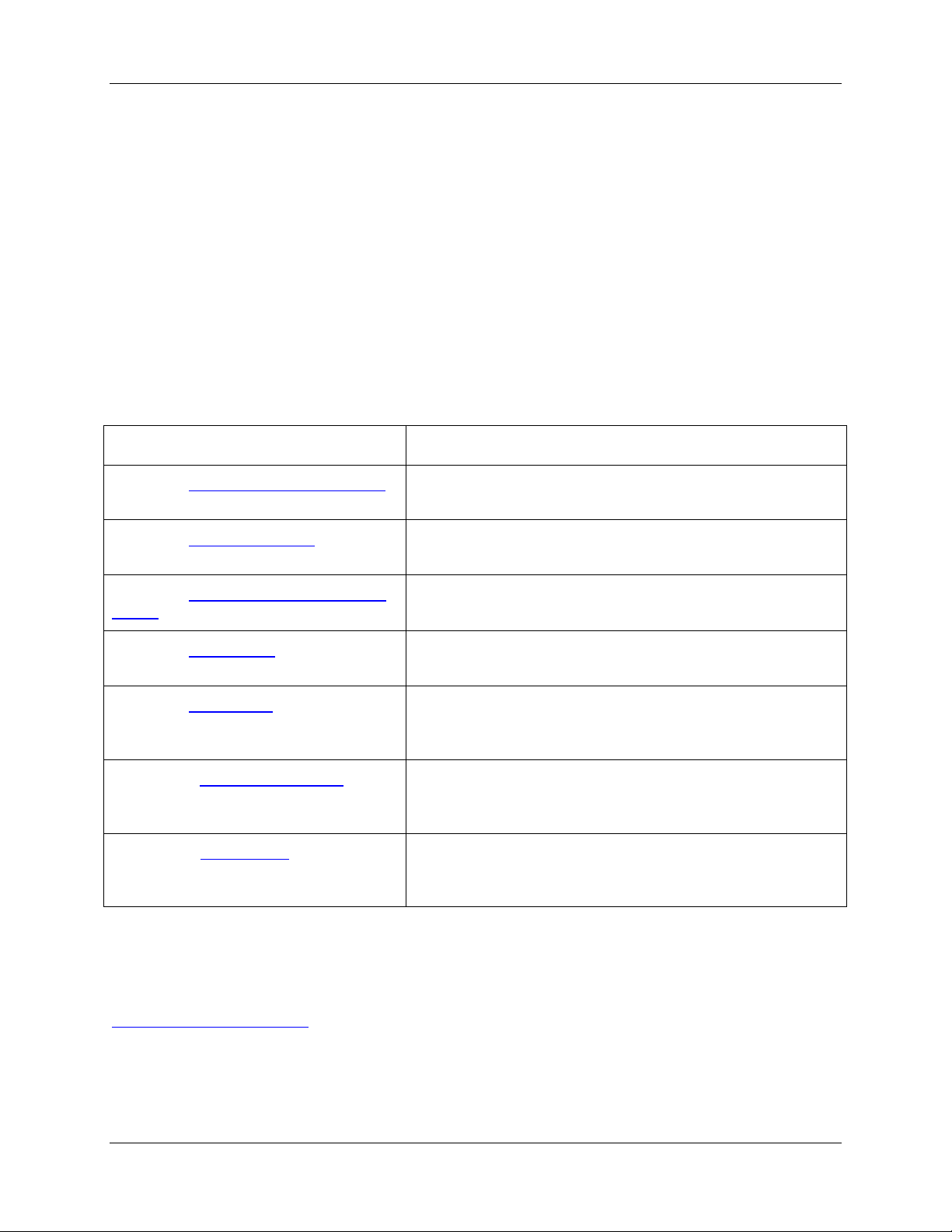
Document Summary

Chapter Description

Chapter 1: Introduction to Spectroscopy

Chapter 2: Overture Software

Chapter 3: Overture Software Icons and

Menus

Chapter 4: Experiments

Chapter 5: Applications

Appendix A: Sample Experiments

Appendix B: Maintenance

Provides an overview of spectroscopy and spectrometers.

Lists installation procedures for Overture software.

Contains a list of the icons and menu items and their
functions in Overture software.

Provides a variety of experiments to perform using Ocean
Optics spectrometers and Overture software.

Contains applications for Overture software.

Contains some possible experiments for Ocean Optics
spectrometers and Overture software.

Provides suggested maintenance and a table of possible
problems and suggested solutions.

Product-Related Documentation

You can access documentation for Ocean Optics products by visiting our website at

http://www.oceanoptics.com

document from the available drop-down lists. Or, use the
of the web page.

000-20000-400-01-201108 v

. Select Technical → Operating Instructions, then choose the appropriate

Search by Model Number field at the bottom

About This Manual

You can also access operating instructions for Ocean Optics products on the Software and Technical
Resources

CD included with the system.

Engineering-level documentation is located on our website at

Technical → Engineering Docs.

Upgrades

Occasionally, you may find that you need Ocean Optics to make a change or an upgrade to your system.
To facilitate these changes, you must first contact Customer Support and obtain a Return Merchandise
Authorization (RMA) number. Please contact Ocean Optics for specific instructions when returning a
product.

vi 000-20000-400-01-201108

Chapter 1

Introduction to Spectroscopy

Spectroscopy in a nutshell

A spectrometer is a device that breaks up light into different colors by spreading out, or dispersing
different wavelengths. Rain does this by refraction
through yellow and then red.

of light, creating a rainbow that goes from violet

This spread of colors is called the visible spectrum. Humans can see light between 380nm (violet) and
780nm (deep red). Other creatures can see different ranges.

You can get the same effect by reflecting light with a CD. The very fine markings on a CD are so small
that they are getting close to the wavelength of light and cause the diffraction of light into a spectrum. The
CD surface is acting as a diffraction grating

000-20000-400-01-201108 1

. In fact it is a reflecting diffraction grating.

Chapter 1: Introduction to Spectroscopy

If you want to find out how a motorcycle works, the best thing to do is take it apart to its individual pieces
and see what it’s made of. The same applies to light. If we can break it up using refraction or diffraction,
we can see what is going on at each wavelength.

Note

Try searching on the web for the words in blue.

Spectroscope views

Below are three spectra as seen through a traditional spectroscope.

This spectrum is of a tungsten filament lamp:

This is spectrum of sunlight. It is a similar continuous spectrum but it contains fine dark lines caused by
absorption of certain wavelengths in the sun and earth atmospheres. These are called Fraunhofer lines

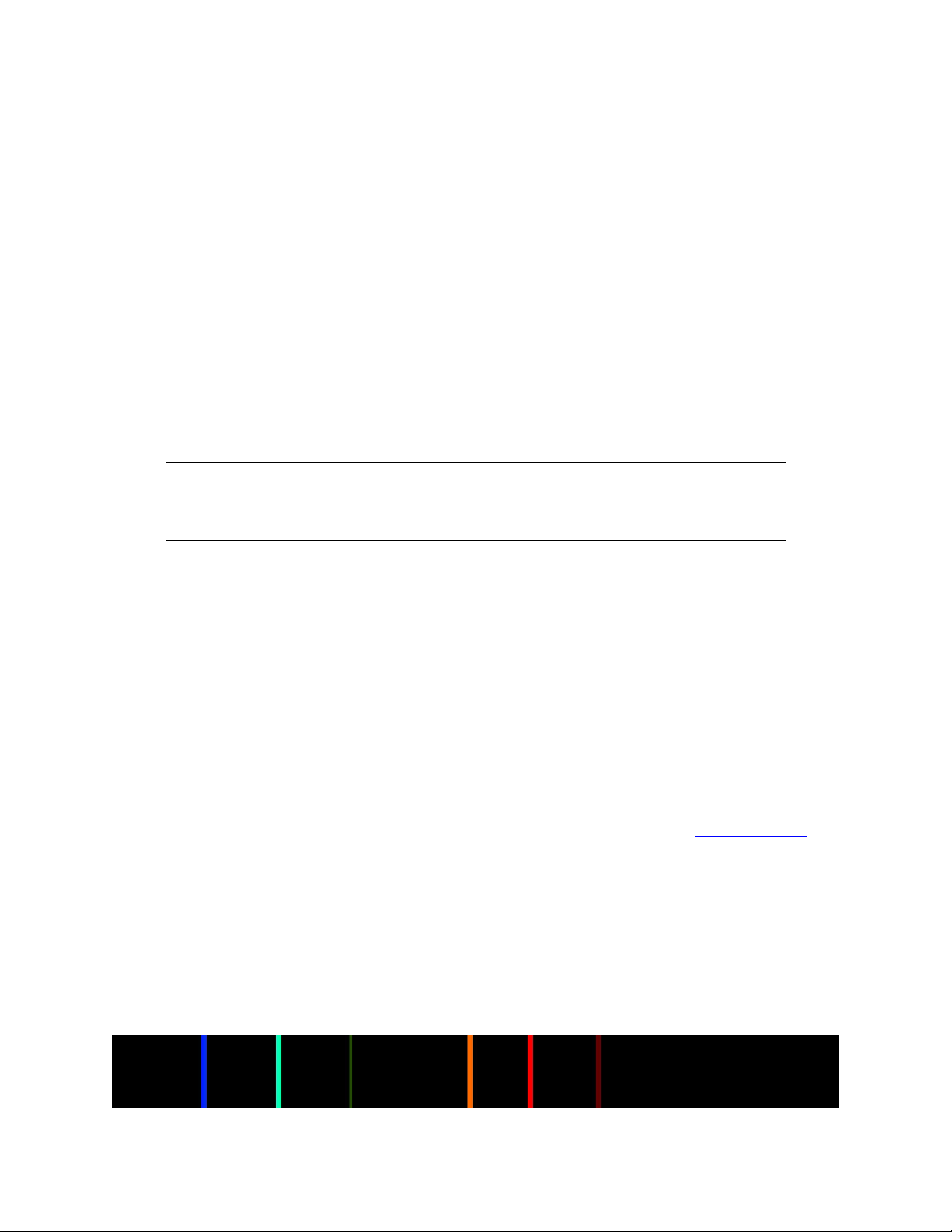
This is an emission spectrum from a hydrogen gas discharge tube. It shows that the hydrogen gas only
emits light at certain wavelengths. Excited hydrogen atoms emit a specific series of narrow spectral lines
called the Balmer series.

.

2 000-20000-400-01-201108

Chapter 1: Introduction to Spectroscopy

The CCD array spectrometer

Looking at sunlight through the spectrometer will tell us a lot about how it works. If you have a pocket
spectroscope you can compare the traditional spectroscope view with the Overture software display.

Sunlight enters the spectrometer through a 50 micron-wide slit. That is very narrow; 5/100ths of a
millimeter.

In a conventional spectroscope you will see a spectrum and any absorbance lines will show as dark lines.
These lines correspond to sharp dips in the Overture spectrum graph.

The light passes through an optical geometry of focusing mirrors and a reflection grating. The spectrum
falls on a linear CCD array
array corresponds to one wavelength.

with 250 tiny sensors in a row so that each sensor (often called a pixel) in the

The number of photons
on the graph. The x-axis is scaled to the pixel number, which indicates wavelength.

hitting each pixel is converted to a voltage which is converted into a y-axis value

Optical Limitations

The Ocean Optics Spectrometers for Education can display peaks separated by less than 2nm, depending
on the model. This is the limit of its resolution.

The spectrometer resolution is limited by a number of factors, including:

 Slit width

 Grating specification (lines per mm) and quality

 Number of pixels in the array

 Physical size of the system

This causes an apparent spreading of emission and absorption lines in the Overture display so that they
appear as sharp Gaussian peaks, but this is still remarkably high resolution for a compact instrument.

In chemistry applications this is not a problem as the absorption peaks are usually over a hundred
nanometers wide. In fact you will deliberately “smooth” the spectrum by averaging the array output using
Overture software.

For chemistry applications it is the sensitivity or dynamic range that is more important. This allows the
spectrometer to detect small changes in absorption on the y-axis.

000-20000-400-01-201108 3

Chapter 1: Introduction to Spectroscopy

Here is what an emission spectrum looks like. This is from a Hydrogen lamp for observing Balmer lines:

Emission lines look like sharp peaks. It is possible to identify elements from their emission peaks. Notice
that some peaks go beyond the visible range.

4 000-20000-400-01-201108

Chapter 2

Overture Software

Product Overview

Overture is a spectroscopy operating software platform for 32-bit and 64-bit Windows. The following
operating systems are supported:

 Windows XP
 Vista
 Windows 7

This software can control the following Ocean Optics spectrometers:

 ADC1000-USB (including Deep Well)
 HR2000
 HR2000+
 HR4000
 Jaz
 Maya2000
 Maya2000Pro
 MMS-Raman
 NIR256
 NIR512
 NIRQuest
 QE65000
 STS
 Torus
 USB2000
 USB2000-FLG
 USB2000+
 USB4000

000-20000-400-01-201108 5

Chapter 2: Overture Software

Overture Installation

Overture can be downloaded from the Ocean Optics Software Downloads site, or retrieved from the CD
that you received with your purchase of an Ocean Optics spectrometer.

Retrieving from a CD

Your Overture software is shipped to you from Ocean Optics on a CD. The software is located either on
the main
separate CD labeled
jacket of the CD containing your SpectraSuite software to complete the installation.

Software and Technical Resources CD, or (in the case of the Windows 64-bit version) on a

Overture Windows 64-bit Version. You will need the password located on the

► Procedure

1. Insert the CD containing your Overture software into your computer.

2. Select the Overture software for your computer’s operating platform via the CD interface. Then
follow the prompts in the installation wizard.

Or,

Browse to the appropriate Overture set-up file for your computer and double-click it to start the
software installation. Set-up files are as follows:

 Windows 32-bit: Overture-windows-x86-1.0.1-installer.exe

 Windows 64-bit: Overture-windows-x64-1.0.1-installer.exe

3. Save the software to the desired location. The default installation directory is

Files\Ocean Optics\Overture

. The installer wizard guides you through the installation process.

Downloading from the Ocean Optics Website

► Procedure

1. Close all other applications running on the computer.

2. Start Internet Explorer.

2. Browse to the Software Downloads page on the Ocean Optics website at

http://www.oceanoptics.com/technical/softwaredownloads.asp.

3. Click on the Overture software appropriate for your Windows operating system.

\Program

4. Save the software to the desired location. The default installation directory is

Files\Ocean Optics\Overture

6 000-20000-400-01-201108

. The installer wizard guides you through the installation process.

\Program

Chapter 3

Overture Software Icons and

Menus

Overview

The following table provides a quick guide to the Overture Software icons. See the paragraphs following
the table for information on how to use these icons when taking a measurement.

000-20000-400-01-201108 7

Chapter 3: Overture Software Icons and Menus

Icon Function

New Graph

Open Spectrum

Save Spectrum

Copy Data to Clipboard

Store Reference Spectrum

Store Dark Spectrum

Intensity

Overture Software Icons

Absorbance

Transmission

Concentration

Snapshot

Wavelength Range

Zoom In

Zoom Out

Print

Reference Lines

Color

8 000-20000-400-01-201108

Chapter 2: Overture Software Icons and Menus

Integration Time

Integration time is the exposure time for each pixel in the array. Each of the pixels is “read” in turn and
the time between readings controls the amount of charge in each CCD sensor. The charge decreases with
every photon that hits the sensor, so if there are not many photons around it takes a long time to reduce
the charge. Too many photons will discharge the sensor completely in a short time.

If the time is too long, the sensors will “saturate” and the spectrum line will go off scale. This does not
harm the sensor, but the data you collect will have no value.

For very dim sources a longer integration time is needed, but the penalty is more noise for less signal. The
default integration time is 100 ms.

The integration time is set in the Integration Time filed in the status bar at the bottom of the screen.

Intensity

Intensity is the default mode.

The y-axis reads Intensity, which is a count of how many photons have hit each pixel in the array during
one integration time. It is a relative measurement.

Intensity mode is ideal for most physics-based applications using just the fiber optic input.

Store Dark Spectrum

Before we can move on to any mathematical comparisons between sample spectra we have to tell the
spectrometer where zero is. To do this, block any light entering the fiber and click the

spectrum

You will not see any change, but the Overture software now has a zero or “dark” reading stored for every
wavelength.

icon.

Store dark

Reference spectrum

Next we have to tell the spectrometer about the source we are comparing to. This is the reference source.
Typically this would be a cuvette containing a colorless solvent, but no dissolved sample.

Set up your reference sample so that the highest point on the intensity y-axis is about 85% of full scale.

Click the store
stored.

Be careful. If you change anything about your reference source now, you must store a new reference. You
can click the icon to update the reference as many times as you like. If you change the integration time
you will need to store a new reference reading.

reference spectrum icon. You will see no change, but your reference spectrum is now

Once you have stored dark and reference spectra, the Transmission and Absorbance modes are enabled.

000-20000-400-01-201108 9

Chapter 3: Overture Software Icons and Menus

Color

Overture can fill the space under the spectrum with an artificial display of spectral color. The color
display covers the visible range of 380nm to 780nm. Outside that range is UV and NIR (near infrared)
and of course we cannot see colors there.

Transmission

Note

Transmission and Absorbance modes are only enabled when dark and reference readings
have been stored.

Transmission is the amount of light transmitted through the sample as a percentage of the light
transmitted through the reference. When you select Transmission mode, the y-axis units change to
percentage.

Where:
Sλ = Sample intensity at wavelength λ
Dλ = Dark intensity at wavelength λ
Rλ = Reference intensity at wavelength λ

So now you can see why you need dark Dλ and reference Rλ readings. If you don’t have them, the math
won’t work!

10 000-20000-400-01-201108

Chapter 2: Overture Software Icons and Menus

Absorbance

Note

Transmission and Absorbance modes are only enabled when dark and reference readings
have been stored.

Absorbance is the amount of light absorbed by the sample compared to the reference.

Absorbance is the inverse of transmission, but on a log scale. When you select Absorbance mode the y­axis changes to a log scale of Absorbance number. So an absorbance number of 1 is 10 times less light
getting through than reference. An absorbance number of two is 100 times less.

Absorbance is normally measured at the wavelength of maximum absorption, called “Lambda Max”,

λ

written
possible to measure Absorbance reliably.

The Absorbance scale goes up to 3. Above 3 the solution is so dark that is no longer

max.

Smoothing

Average scans

This averages over a number of complete scans. For low level light sources this can improve the signal to
noise ratio. For bright sources it is normally not required.

Pixel smoothing

This technique averages a group of adjacent detector elements. A value of 6, for example, averages each
data point with 3 points to its left and 3 points to its right. This average rolls along the array.

The greater this value, the smoother the data. For chemical absorbance experiments a default setting of 5
is set, but this can be changed.

000-20000-400-01-201108 11

Chapter 3: Overture Software Icons and Menus

For absorbance measurements, high resolution is not required, so smoothing makes the spectrum easier to
see and can reduce errors. Setting the pixels to average above 5 is not normally necessary.

Copy Data to Clipboard

The Copy Data tool takes a snapshot of the live spectral data for export as a CSV file into Excel or any
Microsoft Office application.

The data is exported into 2-headed columns in I, A an T modes. The first column is wavelength and the
second column depends on the mode.

Snapshot

Snapshot allows you to freeze as many spectral lines as you want to make comparisons. The frozen lines
can be saved by printing, printing to file or print screen. They will not be saved as spectral data; only the
live spectral line can be saved as a spectrum.

12 000-20000-400-01-201108

Chapter 2: Overture Software Icons and Menus

Zoom

Zoom In lifts the highest peak to the full y axis scale.

Zoom Out cancels this.

Wavelength Range allows you to set both the x and y ranges you want to display. Numerical zoom
can be used in all windows. It is useful to set the wavelength minimum to 400 in Absorbance and
Transmission modes to eliminate the noisy signal that can often be seen at the short wavelength end of the
scale.

Open Spectrum

You can open up to two graphs at the same time and to show two different views, for example,
Absorbance and Transmission at the same time as shown below.

000-20000-400-01-201108 13

Chapter 3: Overture Software Icons and Menus

Cursor

Click anywhere on the graph to launch the cross hairs cursor. The cursor x,y coordinates appear in the
status bar at the bottom right of the screen.

ESC to remove the cursor.

Press

14 000-20000-400-01-201108

Chapter 2: Overture Software Icons and Menus

Reference Lines

Emission lines are referenced using the line spectra library.

Standard spectral lines are taken from NIST data. They are useful for identifying emission peaks from
ionised gases or vapors. The line height is proportional to the relative probability of the transition causing
the emission. Only the strongest lines are shown.

Select the lines you want to display using the check boxes, then click Add or Delete to add them to or
delete them from the list.

The fine green lines are He reference lines. The first thing to notice is that the spectrometer is correctly
calibrated; the lines match the peaks.

000-20000-400-01-201108 15

Chapter 3: Overture Software Icons and Menus

The reference lines are sharp and the real emission lines appear to be not so sharp. The reason for the
broadening is the resolution limits of the spectrometer.

You can use the reference lines to identify elements such as mercury in lamps and metallic elements in
flame tests.

Neon emission lines are closely packed in the yellow and red end of the spectrum. This is why traditional
neon signs have a warm red glow. Different gases produce different colors, so the blue shield is not neon.

16 000-20000-400-01-201108

Menu Functions

Chapter 2: Overture Software Icons and Menus

This section details the various functions available from the Overture menu.

File Menu

The File menu offers the following functions:

 New – Opens the current
 Open
 Save Spectrum
 Print
 Print Setup
 Exit

New

Select this menu item to open the Overture graph in a new screen:

000-20000-400-01-201108 17

Chapter 3: Overture Software Icons and Menus

Open

This menu item allows you to choose whether to show data in a new window or to show data in the
current window.

Save Spectrum

Choose File | Save Spectrum to save a .spec file to a folder on your computer.

Print

Use this menu selection to print your graph. This is the same function that is invoked with the print icon

.

Print Setup

Select Print Setup to choose options for the printer to print your graph.

18 000-20000-400-01-201108

Chapter 2: Overture Software Icons and Menus

Exit

This menu selection allows you shut down Overture.

New

This menu item has one selection: Language. Select Tools | Language to choose to display the Overture
interface from the displayed list.

Window

This menu item provides two options for displaying the graph: Cascade and Tile.

Help

Displays information about Overture.

000-20000-400-01-201108 19

Chapter 3: Overture Software Icons and Menus

20 000-20000-400-01-201108

Chapter 4

Experiments

Concentration wizard

The concentration wizard guides you through the process of measuring absorbance at different
concentrations and plotting a calibration curve to use the Beer-Lambert law to measure unknown
concentrations with the spectrometer system.

The spectrometer can detect very small changes in concentration. The Absorbance number y-axis ranges
from 0 to 3. The ideal working range is between 0.5 and 2.5

► Procedure

1. Set the integration time and smoothing for the reference cuvette. Insert the reference cuvette
into the sampling lamp. Set the integration time so that the peak is at about 85% of maximum.

Set Automatically button will do this for you unless the signal is too far above or below the

The
recommended peak value. In that case, you are asked to set it manually.

000-20000-400-01-201108 21

Chapter 4: Experiments

Note

If you change the integration time or anything else in the experiment setup, you will need
to store new dark and reference readings.

2. Store the dark spectrum. Block the light by turning the mirror. The spectrum line will be flat

and close to the baseline. Click the dark spectrum bulb icon (

). The dark spectrum is now

stored.

3. Store the reference spectrum. Insert the reference cuvette into the sampling lamp. The reference
cuvette should contain only the solvent, usually water or an organic solvent. With a compound in

solution, the absorbance will reduce the peak. Then, click the Reference bulb icon (

st

The line can be displayed in 1
extinction coefficient and R

or 2nd order and forced through the origin. Values for the molar

2

are calculated.

).

22 000-20000-400-01-201108

Chapter 4: Experiments

4. Choose Beer-Lambert Law or Calibration. To use the Beer-Lambert Law option you need to
know the molar absorption (extinction coefficient
trying to find

ε you need to choose the option “Calibrate from solutions of known concentration.”

ε) for the compound you are using. If you are

5. Wavelength range selection. Overture software needs to know which wavelength to measure for
absorbance. Select one (Lambda max) or a range around Lambda max. You can see the
absorbance spectrum behind the dialog box.

000-20000-400-01-201108 23

Chapter 4: Experiments

6. Create the calibration curve. Take at least three samples of known concentration. Either enter
the Absorbance by hand from your notes or scan for it using the
enter the third sample a regression line will be plotted. The line can be displayed in first or second
order and forced through the origin. Values for the molar extinction coefficient and R

Scan now button. When you

2

calculated.

are

7. Concentration meter. Now you can place any unknown concentration of your compound into
the cuvette holder and Overture software will give you an instant reading of the concentration and
show where it sits on the calibration curve with a red diamond marker. No units are shown next to
the reading because you have to know what units you are working in. You can make notes in Step
6 of the units you are working in.

24 000-20000-400-01-201108

Chapter 4: Experiments

Fluorescence

The sampling unit can be set up to measure fluorescence from a side port at 90 degrees to the light path.
Light coming from the sample at 90 degrees has either been scattered or is fluorescence from the sample.
The intensity of fluorescent light is much lower than the in-line light used for absorbance or transmission.
As a result, you need a fiber optic probe with a larger diameter to collect more light. The mirror also helps
to redirect light into the sample to increase the fluorescence.

The Fluorescence fiber (P400-2-VIS/NIR) can be obtained from your supplier.

The following spectra were taken from a fluorescein dye used in a domestic floor cleaner.

000-20000-400-01-201108 25

Chapter 4: Experiments

In transmission mode the same absorbance (now a dip) is seen. We know that light energy is being
absorbed in the 450nm region.

26 000-20000-400-01-201108

Chapter 4: Experiments

The spectrum below is taken from the side port using the fluorescence fiber. It shows a peak at 520 nm .
That is 70nm longer wavelength than the absorption peak. The difference between the absorbance and
fluorescence peaks is about 70nm. The dye is re-emitting light at a longer wavelength. This is called the

Stokes shift

.

000-20000-400-01-201108 27

Chapter 4: Experiments

28 000-20000-400-01-201108

Chapter 5

Applications

Physics applications

The sun

The spectrometer can resolve the strongest Fraunhofer lines. These can be seen in all weather conditions.

000-20000-400-01-201108 29

Chapter 5 Applications

Most of these lines originate from the sun’s chromosphere, but the strong 761nm absorption dip is caused
by Oxygen in our own atmosphere.

Match the Balmer emission lines from the line spectra library to hydrogen absorption lines.

Fluorescent lamps

Strip and compact fluorescent lamps show mercury spectral lines and fluorescence. Use the line spectra
library to identify the mercury

Filters, solutions and glasses

The absorption of near UV rays through sunglasses, optical filters and interference filters. The change in
transmitted wavelength is caused by changing the incident angle of a collimated white light source
through an interference filter.

30 000-20000-400-01-201108

Chapter 5 Applications

Reflection of light from colored surfaces

The spectral emission of scattered light from surfaces shows how surface color depends on absorbed and
reflected light. Illuminate at 90 degrees to the surface and angle the probe at 45 degrees or vice versa.

Ionized gases and metal vapors

Spectrum tubes and lamps produce line spectra. The lines can be used with Planck’s constant to
investigate transition energies and show elementary Overture physics in action. Automotive HID lamps
give a Xenon line emission spectrum.

000-20000-400-01-201108 31

Chapter 5 Applications

Hydrogen spectrum Balmer lines

Calculation of the Rydberg constant from the Balmer series lines. Match to Fraunhofer lines.

Flame emissions

Heating foods that contain sodium or potassium with a hot blue Bunsen flame produces line spectra. Try
potato snacks and a banana. Many foods contain potassium. Now you can find out which ones by
spectroscopic analysis.

32 000-20000-400-01-201108

Chapter 5 Applications

Standard flame test compounds can be used to show how all the metallic elements produce line spectra.
Sodium contamination is less of a problem as the Na line can be identified and does not affect other lines.
The spectrometer “sees” discrete wavelengths, so even if you can’t see a line behind a yellow sodium
glow, the spectrometer can.

Lasers

Lasers have a near-monochromatic line spectrum (sharp Gaussian). Some of the Gaussian spread is
caused by the spectrometer. The sharper the line the more monochromatic the light. Compare this with
LEDs, interference and gel filters.

000-20000-400-01-201108 33

Chapter 5 Applications

Chemistry applications

Following are some of the color-related experiments that can be carried out with your spectrometer
system.

Spectral signatures

Chlorophylls and food colorings in solution can be identified by their absorbance ‘fingerprint’.

Olive oils of different quality show very different absorption depending on the amount of chlorophyll
they contain.

Flame tests

The spectrometer detects sharp emission peaks even when these are invisible to the human eye.

Multiple elements can be observed. This reinforces understanding of advanced spectroscopic techniques
that show multiple peaks.

Common foods like potato snacks and dried banana chips show distinct emission peaks when heated.
Bananas show a potassium doublet. Salted snacks show sodium and some containing LoSalt (Potassium
Chloride) show a strong potassium line.

The problem of sodium contamination is removed because the spectrometer is a polychromator and sees
all wavelengths at the same time. The sensitivity and speed of the spectrometer allows momentary
emission spectra to be recorded using the snapshot tool.

Transmission, absorbance and the concept of Absorbance
Number

Transmission % = (Sλ – Dλ / Rλ – Dλ) x 100

Absorbance = - log10 (S

Beers law using KMnO

λ – Dλ / Rλ – Dλ)

4

Determination of the pKa of bromocresol green

Finding the isosbestic point using the snapshot tool.

34 000-20000-400-01-201108

Chapter 5 Applications

Spectrophotometric analysis of commercial aspirin

Acetyl Salicylic Acid (ASA) complex ion is formed by hydrolyzing the ASA or aspirin sample in NaOH
solution and complexing it with Fe3+ ion in acid solution to bring out the color with a maximum
absorption at a wavelength of 530 nm.

Spectrophotometric determination of an equilibrium
constant

Investigating the reaction between aqueous solutions of iron (III) nitrate, Fe(NO3)3, and potassium
thiocyanate, KSCN. The reaction produces the blood-red complex FeSCN2+. The reaction also
establishes an equilibrium allowing the equilibrium constant to be obtained by sampling multiple
reactions using different concentrations.

Water quality testing using indicator reagents

Phosphate and Nitrate concentrations can be accurately measured by analysis of the absorbance of
solutions using commercial testing reagents.

000-20000-400-01-201108 35

Chapter 5 Applications

36 000-20000-400-01-201108

Appendix A

Sample Experiments

Beer’s law analysis of KMnO

Equipment Needed:

 Ocean Optics CCD array spectrometer with lamp/cuvette holder

 Equipment for making aqueous solutions of different concentrations of KMnO

 Cuvettes

Objectives:

 To find the molar absorbance coefficient (ε) for potassium permanganate, potassium manganate

(VII), by plotting a calibration curve using the Beer Lambert Law.

 Using the calibration to find the concentration of an unknown sample.

Procedure:

1. Set the spectrometer in A (Absorbance) mode.

2. Click on the concentration wizard icon before setting dark and reference readings. The wizard will
help you set the correct integration time.

4

4

3. From a stock solution of known concentration in Moles per liter, make up a range of dilutions of at
least three precisely known concentrations. Use solutions which have absorbance numbers between

0.5 and 2.5.

4. Measure these solutions in A mode. Potassium permanganate has a very high molar absorbance
coefficient (ε), so solutions have to be very dilute. As Absorbance numbers reach 3, Beers Law starts
to become less reliable.

5. Find

000-20000-400-01-201108 37

λ max. For potassium permanganate this should be about 534nm (you will see two peaks at 524

and 544nm).

Appendix A: Sample Experiments

6. In the Concentration Wizard, select “Calibrate from solutions of known concentration”.

7. In the Range selection,

8. Enter at least three concentration values and scan for Absorbance in each case. On the third data point
the wizard will plot a regression line. Add more samples if you have them.

9. Clicking Finish will convert the spectrometer into a concentration meter that uses the calibration line
that you have made. Use the meter to measure unknown concentrations.

Other Beers Law Experiments:

 Use food dyes and measure unknown concentrations in food products. For example, measure

Erythrosin B In Maraschino cherries.

 Use water quality indicator reagents to measure concentrations of nitrates in water samples.

set the wavelength at λ max or average across the peak.

Chlorophyll detection in olive oils

Equipment Needed:

 Ocean Optics CCD array spectrometer with lamp cuvette holder

 Three grades of olive oil

 Cuvettes

38 000-20000-400-01-201108

Appendix A: Sample Experiments

 Flasks, beakers and pipettes for preparation

Objectives:

Olive oils contain varying amounts of chlorophyll, depending on the grades: extra virgin, standard and
light. This experiment will show qualitatively how the grades compare and can be extended to compare
with chlorophyll extracted from green leaves with isopropanol.

Procedure:

1. For a reference spectrum, water can be used. There is a discussion point about what a reference
should be for an experiment with oils, since there is no solvent as such.

2. Take reference and dark readings and set Overture to Absorbance mode. If necessary, use numerical
zoom to cut of the noisy signal below 400 nm.

3. Visible absorbance peaks for chlorophyll are at: 413, 454, and 482 nm, 631 and 669 nm. See how
many you can detect

.

Flame tests

Equipment Needed:

 Ocean Optics CCD array spectrometer with 400 micron fiber optic cable

000-20000-400-01-201108 39

Appendix A: Sample Experiments

 Stand and clamp

 Flame test wire loop

 Banana or dried banana chips

 Salts: LiCl, NaCl, SrCl2, CuCl2, BaCl2, CaCl2

 1M HCl for cleaning the loop

Objectives:

 To show that flames test emissions are line spectra that can be identified by comparison with

reference line spectra.

 To use potassium salts and the reference library of emission lines to identify potassium in

bananas.

Procedure:

1. Set the spectrometer to Intensity mode. Use a 400 micron fiber optic or remove the fiber optic cable.

Caution

If you use the spectrometer without a fiber optic cable, you should take steps to
prevent chemicals from entering the entrance port. Use a small piece of plastic wrap
to cover the port.

2. Hold the fiber in a laboratory clamp about 30 cm from the flame.

3. Be careful not to have fluorescent lamps in the line of sight of the fiber. This will cause mercury
spectral lines. Use the mercury lines to check for these.

4. Use the Snapshot tool to freeze spectral lines.

5. Overlay the reference lines to identify the metal elements in salts.

Sodium contamination will show up as a line at 589nm.You can try to clean the flame test loop with HCl
to eliminate it, or just recognize it as contamination. Sodium contamination is a problem when looking at
flames by eye because the yellow is so bright that it masks other fainter colors. The spectrometer does not
have that problem because every wavelength is detected and displayed separately.

40 000-20000-400-01-201108

Appendix A: Sample Experiments

Spectrophototmetric analysis of a buffer
solution – Isobestic point

Procedure:

1. Measure and analyze the visible light absorbance spectrum of an acetate buffer solution containing
bromocresol green indicator.

2. Compare the spectra of a sample of acetate buffer that has been treated with acid to a sample of the
buffer treated with base.

3. Use test results to calculate the pH of the buffer solution.

000-20000-400-01-201108 41

Appendix A: Sample Experiments

Fluorescence and Stokes shift

Objectives:

Using the side port of the sampling unit the Stokes shift of fluorescent compounds in solution can be
measured.

Procedure:

1. Using an open bench set up and a UV lamp you can detect fluorescence by pointing the fiber at the
side of the cuvette.

2. Visible fluorescence of fluorescein from UV excitation by a UV led can be measured. This
phenomenon is used by opticians to show up scratches on the cornea and is the basis of confocal
microscopy used to view biological samples.

42 000-20000-400-01-201108

Appendix B

Maintenance

Fiber care

The fiber optic cables have a glass core. They should not be bent with a radius of less than 10cm.

If the fiber ends become dirty, use a lens wipe and alcohol to clean gently.

Always keep the protective caps on when not in use.

Spectrometer care

Ocean Optics spectrometers are precision instruments designed as light, portable devices. Take the
following precautions:

 Avoid shocks and drops

 Avoid extremes of temperature

 If exposed to sub zero temperatures allow to reach room temperature and wait for one hour before

operating

 Avoid prolonged exposure to direct sunlight

 Always replace dust caps when not in use

000-20000-400-01-201108 43

Appendix B: Maintenance

Troubleshooting

Problem Possible Cause(s) Suggested Solution(s)

The icons are grayed-out USB cable is not firmly

connected.

The trace is very low Too little light

Zoom – is set.

The trace is off the intensity
scale

The low wavelength trace in
Absorbance mode or
Transmission mode is spiky
and jumpy.

There are unexpected sharp
peaks in the spectrum.

Too much light

Zoom + is set

At below 400nm the sampling unit
lamp has a low intensity. In
Absorbance and Transition
modes, the signal to noise ratio is
too low to give a reliable signal.

There is a fluorescent lamp in the
vicinity.

Close the Overture software,
recheck the USB connection, then
re-open the software.

Increase the integration time.
Position the fiber to receive more
light.

Try Zoom+ or numerical zoom on
the y-axis.

Reduce the integration time.
Position the fiber to receive less
light.

Click Zoom –

Use numerical zoom to start the x­axis at 450nm.

Remove or turn off fluorescent
lamps in the lab. These emit sharp
mercury spectral lines.

The fluorescent signal from the
side fiber connector is very
weak.

Incorrect fiber is being used. Make sure you have the P-400-2-

VIS-NIR micron fiber connected to
the side port.

FAQs

How can I get software upgrades?

These are available from your distributor. Software upgrades are free.

How strong is the fiber optic cable?

The fiber core is made of glass. Do not bend the fiber sharply with a radius of less than 10cm.

44 000-20000-400-01-201108

Appendix B: Maintenance

Can I use the spectrometer outside?

Yes, but only in dry, warm conditions. Do not expose the case to direct sunlight. The spectrometer is a
laboratory instrument and not designed to operate in a harsh environment.

I have spilled chemicals in the cuvette holder. What should I do?

1. Use the hex key to remove the lamp module.

2. Clean the lamp with a soft damp cloth.

3. Wash out the cuvette holder with de-ionized water.

4. Air dry. Reassemble.

Where can I buy the 400 micron Fluorescence fiber?

These are available from your distributor.

I am looking at low level light sources. How can I get more light into the spectrometer?

Use the 400 micron fiber. This lets in about ten times as much light as the 50 micron fiber.
Alternatively use without the fiber, but keep the dust cap on when not in use.

How do I calibrate my spectrometer?

Ocean Optics spectrometers are factory calibrated. A severe shock could cause a calibration error, but in
normal use the spectrometer should never require re-calibration. You can check calibration against the
library of emission spectra.
Contact you distributor if you have a problem.

000-20000-400-01-201108 45

Appendix B: Maintenance

46 000-20000-400-01-201108

Index

A

absorbance

mode, 11
number, 34

applications, 29

chemistry, 34
physics, 29

average scans, 11

B

Balmer lines, 32
Beers Law, 34
Beer's law analysis of KMno

, 37

4

C

chemistry applications, 34

absorbance, 34
Beers Law, 34
flame tests, 34
isosbestic, 34
spectral signatures, 34
spectrophotometric analysis of aspirin, 35
spectrophotometric analysis of equilibrium
constant, 35

water quality testing, 35
Chlorophyll detection in olive oils, 38
color fill, 10
concentration, 21
copy data to clipboard, 12
cursor, 14

D

dark spectrum, 9
document

audience, v

purpose, v

summary, v
documentation, v

E

emission spectrum, 4
Exit, 19
experiment, 21

concentration, 21
fluorescence, 25

experiments, 37

Beer's law analysis of KMno
Chlorophyll detection in olive oils, 38
flame tests, 39
fluorescence and Stokes shift, 42
Spectrophototmetric analysis of a buffer
solution, 41

, 37

4

F

FAQs, 44
fiber care, 43
File menu, 17
filters, 30
flame

emissions, 32

tests, 34
flame tests, 39
fluorescence, 25
fluorescence and Stokes shift, 42
fluorescent lamp, 30

G

glasses, 30

H

Help menu, 19
hydrogen spectrum, 32

000-20000-400-01-201108 47

I

icons, 8
installation, 5

via CD, 6

via download, 6
integration time, 9
intensity mode, 9
ionized gases, 31
isosbestic, 34

L

lasers, 33

M

menu

File, 17

Help, 19

New, 19

Window, 19
menu functions, 17
metal vapors, 31

N

New, 17
New menu, 19
new spectrum window, 13

O

pixel smoothing, 11
Print, 18
Print Setup, 18

R

reference

lines, 15
spectrum, 9

reflection, 31

S

Save Spectrum, 18
smoothing, 11

average scans, 11

pixel, 11
snapshot, 12
solutions, 30
spectra library, 15
spectral signatures, 34
spectrometer, 3

care, 43

optical limitations, 3
spectrophotometric

analysis of aspirin, 35

analysis of equilibrium constant, 35
Spectrophototmetric analysis of a buffer
solution, 41
spectroscope views, 2
spectroscopy, 1
sun, 29

Open, 18
optical limitations, 3

transmission, 34

P

physics applications, 29

filters, 30
flame emissions, 32
fluorescent lamp, 30
glasses, 30
hydrogen specrum, 32
ionized gases, 31
lasers, 33
metal vapors, 31
reflection, 31
solutions, 30
sun, 29

48 000-20000-400-01-201108

mode, 10
troubleshooting, 44

upgrades, vi

water quality testing, 35
Window menu, 19

zoom, 13

T

U

W

Z