Casio FX-9860GI SLIM - SOFTWARE VERSION 2-00, FX-7400GII - SOFTWARE VERSION 2-00, fx-9750GII, FX-9860G - SOFTWARE VERSION 2-00, fx-9860G User Manual

...

Download

CASIO Worldwide Education Website

http://edu.casio.com

CASIO EDUCATIONAL FORUM

http://edu.casio.com/forum/

fx-9860GII SD fx-9860GII fx-9860G AU PLUS fx-9860G Slim

(Updated to OS 2.00)

fx-9860G SD (Updated to OS 2.00) fx-9860G (Updated to OS 2.00) fx-9860G AU (Updated to OS 2.00)

I[*ɉ I[*ɉ

Software Version 2.00

User’s Guide

• The contents of this user’s guide are subject to change without notice.

• No part of this user’s guide may be reproduced in any form without the express written consent of the manufacturer.

• The options described in Chapter 13 of this user’s guide may not be available in certain geographic areas. For full details on availability in your area, contact your nearest CASIO dealer or distributor.

• Be sure to keep all user documentation handy for future reference.

Contents

Getting Acquainted — Read This First!

Chapter 1 Basic Operation

1. Keys .............................................................................................................................. 1-1

2. Display .......................................................................................................................... 1-2

3. Inputting and Editing Calculations.................................................................................1-5

4. Using the Math Input/Output Mode ............................................................................. 1-10

5. Option (OPTN) Menu .................................................................................................. 1-22

6. Variable Data (VARS) Menu ....................................................................................... 1-23

7. Program (PRGM) Menu ............................................................................................. 1-25

8. Using the Setup Screen .............................................................................................. 1-26

9. Using Screen Capture.................................................................................................1-29

10. When you keep having problems… ........................................................................... 1-30

Chapter 2 Manual Calculations

1. Basic Calculations.........................................................................................................2-1

2. Special Functions..........................................................................................................2-6

3. Specifying the Angle Unit and Display Format............................................................2-10

4. Function Calculations..................................................................................................2-11

5. Numerical Calculations ............................................................................................... 2-21

6. Complex Number Calculations.................................................................................... 2-30

7. Binary, Octal, Decimal, and Hexadecimal Calculations with Integers......................... 2-33

8. Matrix Calculations......................................................................................................2-36

9. Mertic Conversion Calculations................................................................................... 2-48

Chapter 3 List Function

1. Inputting and Editing a List............................................................................................ 3-1

2. Manipulating List Data................................................................................................... 3-5

3. Arithmetic Calculations Using Lists ............................................................................. 3-10

4. Switching Between List Files....................................................................................... 3-13

Chapter 4 Equation Calculations

1. Simultaneous Linear Equations .................................................................................... 4-1

2. High-order Equations from 2nd to 6th Degree .............................................................. 4-2

3. Solve Calculations......................................................................................................... 4-4

Chapter 5 Graphing

1. Sample Graphs .............................................................................................................5-1

2. Controlling What Appears on a Graph Screen.............................................................. 5-2

3. Drawing a Graph ........................................................................................................... 5-6

4. Storing a Graph in Picture Memory............................................................................. 5-10

5. Drawing Two Graphs on the Same Screen................................................................. 5-11

6. Manual Graphing......................................................................................................... 5-12

7. Using Tables ...............................................................................................................5-15

8. Dynamic Graphing ...................................................................................................... 5-20

9. Graphing a Recursion Formula ................................................................................... 5-22

10. Graphing a Conic Section ...........................................................................................5-27

11. Changing the Appearance of a Graph ........................................................................ 5-27

12. Function Analysis ........................................................................................................ 5-29

iii

Chapter 6 Statistical Graphs and Calculations

1. Before Performing Statistical Calculations .................................................................... 6-1

2. Calculating and Graphing Single-Variable Statistical Data ...........................................6-4

3. Calculating and Graphing Paired-Variable Statistical Data ........................................... 6-9

4. Performing Statistical Calculations .............................................................................. 6-15

5. Tests ........................................................................................................................... 6-22

6. Confidence Interval ..................................................................................................... 6-35

7. Distribution ..................................................................................................................6-38

8. Input and Output Terms of Tests, Confidence Interval, and Distribution .................... 6-50

9. Statistic Formula ......................................................................................................... 6-53

Chapter 7 Financial Calculation (TVM)

1. Before Performing Financial Calculations ..................................................................... 7-1

2. Simple Interest .............................................................................................................. 7-2

3. Compound Interest ........................................................................................................ 7-3

4. Cash Flow (Investment Appraisal) ................................................................................7-5

5. Amortization ..................................................................................................................7-7

6. Interest Rate Conversion .............................................................................................. 7-9

7. Cost, Selling Price, Margin .......................................................................................... 7-10

8. Day/Date Calculations ................................................................................................. 7-11

9. Depreciation ................................................................................................................ 7-12

10. Bond Calculations ....................................................................................................... 7-14

11. Financial Calculations Using Functions ...................................................................... 7-16

Chapter 8 Programming

1. Basic Programming Steps ............................................................................................. 8-1

2. PRGM Mode Function Keys .......................................................................................... 8-2

3. Editing Program Contents ............................................................................................. 8-3

4. File Management .......................................................................................................... 8-5

5. Command Reference ....................................................................................................8-7

6. Using Calculator Functions in Programs ..................................................................... 8-21

7. PRGM Mode Command List ....................................................................................... 8-37

8. Program Library .......................................................................................................... 8-42

Chapter 9 Spreadsheet

1. Spreadsheet Basics and the Function Menu ................................................................ 9-1

2. Basic Spreadsheet Operations ..................................................................................... 9-2

3. Using Special S • SHT Mode Commands .................................................................... 9-14

4. Drawing Statistical Graphs, and Performing Statistical and Regression

Calculations ................................................................................................................. 9-15

5. S • SHT Mode Memory ................................................................................................9-20

Chapter 10 eActivity

1. eActivity Overview ....................................................................................................... 10-1

2. eActivity Function Menus ............................................................................................10-2

3. eActivity File Operations ............................................................................................. 10-3

4. Inputting and Editing Data ........................................................................................... 10-4

5. eActivity Guide .......................................................................................................... 10-13

Chapter 11 Memory Manager

1. Using the Memory Manager ........................................................................................ 11-1

Chapter 12 System Manager

1. Using the System Manager ......................................................................................... 12-1

2. System Settings .......................................................................................................... 12-1

Chapter 13 Data Communications

1. Connecting Two Units ................................................................................................. 13-1

2. Connecting the Calculator to a Personal Computer .................................................... 13-1

3. Performing a Data Communication Operation ............................................................13-2

4. Data Communications Precautions ............................................................................. 13-5

5. Screen Image Send .................................................................................................. 13-11

Chapter 14 Using SD Cards (fx-9860GⅡ SD only)

1. Using an SD Card .......................................................................................................14-1

2. Formatting an SD Card ...............................................................................................14-3

3. SD Card Precautions during Use ................................................................................ 14-3

Appendix

1. Error Message Table .................................................................................................... A-1

2. Input Ranges ................................................................................................................A-5

E-CON2 Application

1 E-CON2 Overview 2 Using the Setup Wizard 3 Using Advanced Setup 4 Using a Custom Probe 5 Using the MULTIMETER Mode 6 Using Setup Memory 7 Using Program Converter 8 Starting a Sampling Operation 9 Using Sample Data Memory 10 Using the Graph Analysis Tools to Graph Data 11 Graph Analysis Tool Graph Screen Operations 12 Calling E-CON2 Functions from an eActivity

Getting Acquainted — Read This First!

I About this User’s Guide

S Model-specific Function and Screen Differences

This User’s Guide covers multiple different calculator models. Note that some of the functions described here may not be available on all of the models covered by this User’s Guide. All of the screen shots in this User’s Guide show the fx-9860G

ɉ SD screen, and the appearance of

the screens of other models may be slightly different.

S Math natural input and display

Under its initial default settings, the fx-9860Gɉ SD, fx-9860Gɉ, or fx-9860G AU PLUS is set up to use the “Math input/output mode”, which enables natural input and display of math expressions. This means you can input fractions, square roots, differentials, and other expressions just as they are written. In the “Math input/output mode”, most calculation results also are displayed using natural display.

You also can select a “Linear input/output mode” if you like, for input and display of calculation expressions in a single line. The initial default setting of the fx-9860G

ɉ SD, fx-

9860Gɉ, and fx-9860G AU PLUS input/output mode is the Math input/output mode. The examples shown in this User’s Guide are mainly presented using the Linear input/output

mode. Note the following points if you are using an fx-9860G

ɉ SD, fx-9860Gɉ, or fx-9860G

AU PLUS.

• For information about switching between the Math input/output mode and Linear input/ output mode, see the explanation of the “Input/Output” mode setting under “Using the Setup Screen” (page 1-26).

• For information about input and display using the Math input/output mode, see “Using the Math Input/Output Mode” (page 1-10).

S For owners of models not equipped with a Math input/output mode

(fx-7400G

ɉ, fx-9750Gɉ)...

The fx-7400Gɉ and fx-9750Gɉ do not include a Math input/output mode. When performing the calculations in this manual on these models, use the linear input mode. fx-7400Gɉ and fx-9750Gɉ owners should ignore all explanations in this manual concerned with the Math input/output mode.

S V()

The above indicates you should press  and then V, which will input a  symbol. All multiple-key input operations are indicated like this. Key cap markings are shown, followed by the input character or command in parentheses.

S K EQUA

This indicates you should first press K, use the cursor keys (D, A, B, C) to select the EQUA mode, and then press U. Operations you need to perform to enter a mode from the Main Menu are indicated like this.

S Function Keys and Menus

• Many of the operations performed by this calculator can be executed by pressing function keys  through . The operation assigned to each function key changes according to

the mode the calculator is in, and current operation assignments are indicated by function menus that appear at the bottom of the display.

• This User’s Guide shows the current operation assigned to a function key in parentheses following the key cap for that key. (Comp), for example, indicates that pressing  selects {Comp}, which is also indicated in the function menu.

• When (E) is indicated in the function menu for key , it means that pressing  displays the next page or previous page of menu options.

S Menu Titles

• Menu titles in this User’s Guide include the key operation required to display the menu being explained. The key operation for a menu that is displayed by pressing * and then {LIST} would be shown as: [OPTN]-[LIST].

• (E) key operations to change to another menu page are not shown in menu title key operations.

S Command List

The PRGM Mode Command List (page 8-37) provides a graphic flowchart of the various function key menus and shows how to maneuver to the menu of commands you need.

Example: The following operation displays Xfct: [VARS]-[FACT]-[Xfct]

S E-CON2

This manual does not cover the E-CON2 mode. For more information about the E-CON2 mode, download the E-CON2 manual (English version only) from: http://edu.casio.com.

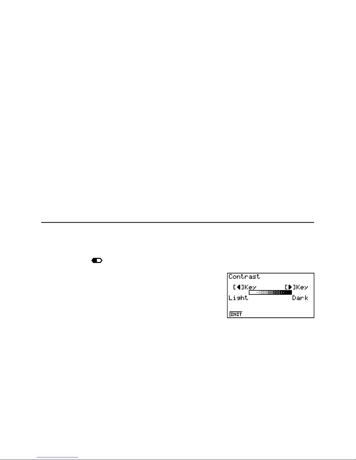
I Contrast Adjustment

Adjust the contrast whenever objects on the display appear dim or difficult to see.

1. Use the cursor keys (D, A, B, C) to select the SYSTEM icon and press U, then press (

) to display the contrast adjustment screen.

2. Adjust the contrast.

• The C cursor key makes display contrast darker.

• The B cursor key makes display contrast lighter.

• (INIT) returns display contrast to its initial default.

3. To exit display contrast adjustment, press K.

1-1

Chapter 1 Basic Operation

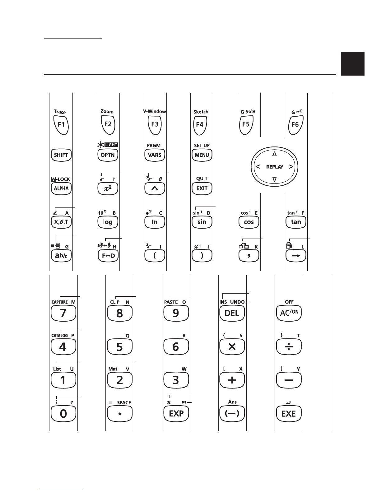
1. Keys

I Key Table

Not all of the functions described above are available on all models covered by this manual. Depending on calculator model, some of the above keys may not be included on your calculator.

Page Page Page Page Page Page

Page Page Page Page Page

2-1

5-29 5-5 5-3

2-14

1-18, 2-14

1-2

2-7

2-14 2-14

5-28 5-30 5-1

5-24

1-25 1-26

1-2 1-22 1-23 1-2

2-14

2-13

2-13 2-13

2-1

1-12 1-18 2-19

2-1

2-6

2-30

1-11

1-19 2-19

2-19

1-16 1-6

2-1

2-9 2-1

1-6,1-15

2-1

1-9

2-13 2-7

1-8

2-41

1-30

1-9

3-2

2-30

10-11 10-9

Page Page Page Page Page Page

Page Page Page Page Page

2-1

5-29 5-5 5-3

2-14

1-18, 2-14

1-2

2-7

2-14 2-14

5-28 5-30 5-1

5-24

1-25 1-26

1-2 1-22 1-23 1-2

2-14

2-13

2-13 2-13

2-1

1-12 1-18 2-19

2-1

2-6

2-30

1-11

1-19 2-19

2-19

1-16 1-6

2-1

2-9 2-1

1-6,1-15

2-1

1-9

2-13 2-7

1-8

2-41

1-30

1-9

3-2

2-30

10-11 10-9

1-2

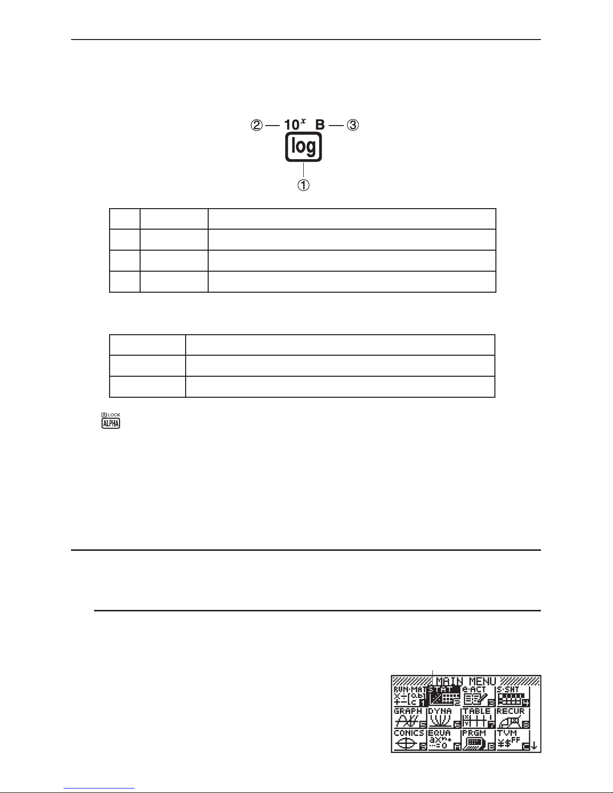
I Key Markings

Many of the calculator’s keys are used to perform more than one function. The functions marked on the keyboard are color coded to help you find the one you need quickly and easily.

Function Key Operation



log



J



The following describes the color coding used for key markings.

Color Key Operation

Yellow

Press  and then the key to perform the marked function.

Red

Press ? and then the key to perform the marked function.

•

Alpha Lock

Normally, once you press ? and then a key to input an alphabetic character, the keyboard reverts to its primary functions immediately. If you press  and then ?, the keyboard locks in alpha input until you press ? again.

2. Display

I Selecting Icons

This section describes how to select an icon in the Main Menu to enter the mode you want.

S To select an icon

1. Press K to display the Main Menu.

2. Use the cursor keys (B, C, D, A) to move the highlighting to the icon you want.

Currently selected iconCurrently selected icon

1-3

3. Press U to display the initial screen of the mode whose icon you selected. Here we will enter the STAT mode.

• You can also enter a mode without highlighting an icon in the Main Menu by inputting the

number or letter marked in the lower right corner of the icon.

• Use only the procedures described above to enter a mode. If you use any other procedure,

you may end up in a mode that is different than the one you thought you selected.

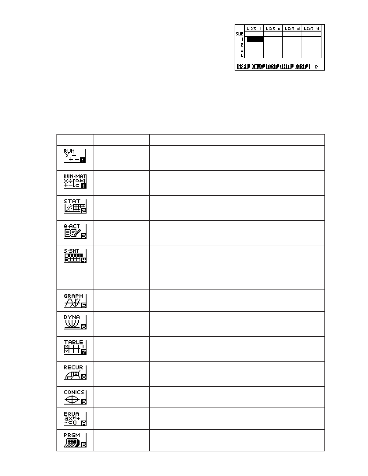
The following explains the meaning of each icon.

Icon Mode Name Description

RUN (fx-7400Gɉ only)

Use this mode for arithmetic calculations and function calculations, and for calculations involving binary, octal, decimal, and hexadecimal values.

RUN • MAT*

(Run • Matrix)

Use this mode for arithmetic calculations and function calculations, and for calculations involving binary, octal, decimal, and hexadecimal values and matrices.

STAT (Statistics)

Use this mode to perform single-variable (standard deviation) and paired-variable (regression) statistical calculations, to perform tests, to analyze data and to draw statistical graphs.

e • ACT*

(eActivity)

eActivity lets you input text, math expressions, and other data in a notebook-like interface. Use this mode when you want to store text or formulas, or built-in application data in a file.

S • SHT*

(Spreadsheet)

Use this mode to perform spreadsheet calculations. Each file contains a 26-column × 999-line spreadsheet. In addition to the calculator’s built-in commands and S • SHT mode commands, you can also perform statistical calculations and graph statistical data using the same procedures that you use in the STAT mode.

GRAPH Use this mode to store graph functions and to draw graphs

using the functions.

DYNA*

(Dynamic Graph)

Use this mode to store graph functions and to draw multiple versions of a graph by changing the values assigned to the variables in a function.

TABLE Use this mode to store functions, to generate a numeric table

of different solutions as the values assigned to variables in a function change, and to draw graphs.

RECUR*

(Recursion)

Use this mode to store recursion formulas, to generate a numeric table of different solutions as the values assigned to variables in a function change, and to draw graphs.

CONICS*

Use this mode to draw graphs of conic sections.

EQUA (Equation)

Use this mode to solve linear equations with two through six unknowns, and high-order equations from 2nd to 6th degree.

PRGM (Program)

Use this mode to store programs in the program area and to run programs.

1-4

Icon Mode Name Description

TVM*

(Financial)

Use this mode to perform financial calculations and to draw cash flow and other types of graphs.

E-CON2*

Use this mode to control the optionally available EA-200 Data Analyzer. For more information about the E-CON2 mode, download the E-CON2 manual (English version only) from: http://edu.casio. com.

LINK Use this mode to transfer memory contents or back-up data to

another unit or PC.

MEMORY Use this mode to manage data stored in memory.

SYSTEM Use this mode to initialize memory, adjust contrast, and to

make other system settings.

*1 Not included on the fx-7400Gɉ. *2 Not included on the fx-7400Gɉ/fx-9750Gɉ.

I About the Function Menu

Use the function keys ( to ) to access the menus and commands in the menu bar along the bottom of the display screen. You can tell whether a menu bar item is a menu or a command by its appearance.

I About Display Screens

This calculator uses two types of display screens: a text screen and a graph screen. The text screen can show 21 columns and 8 lines of characters, with the bottom line used for the function key menu. The graph screen uses an area that measures 127 (W) × 63 (H) dots.

Text Screen Graph Screen

I Normal Display

The calculator normally displays values up to 10 digits long. Values that exceed this limit are automatically converted to and displayed in exponential format.

S How to interpret exponential format

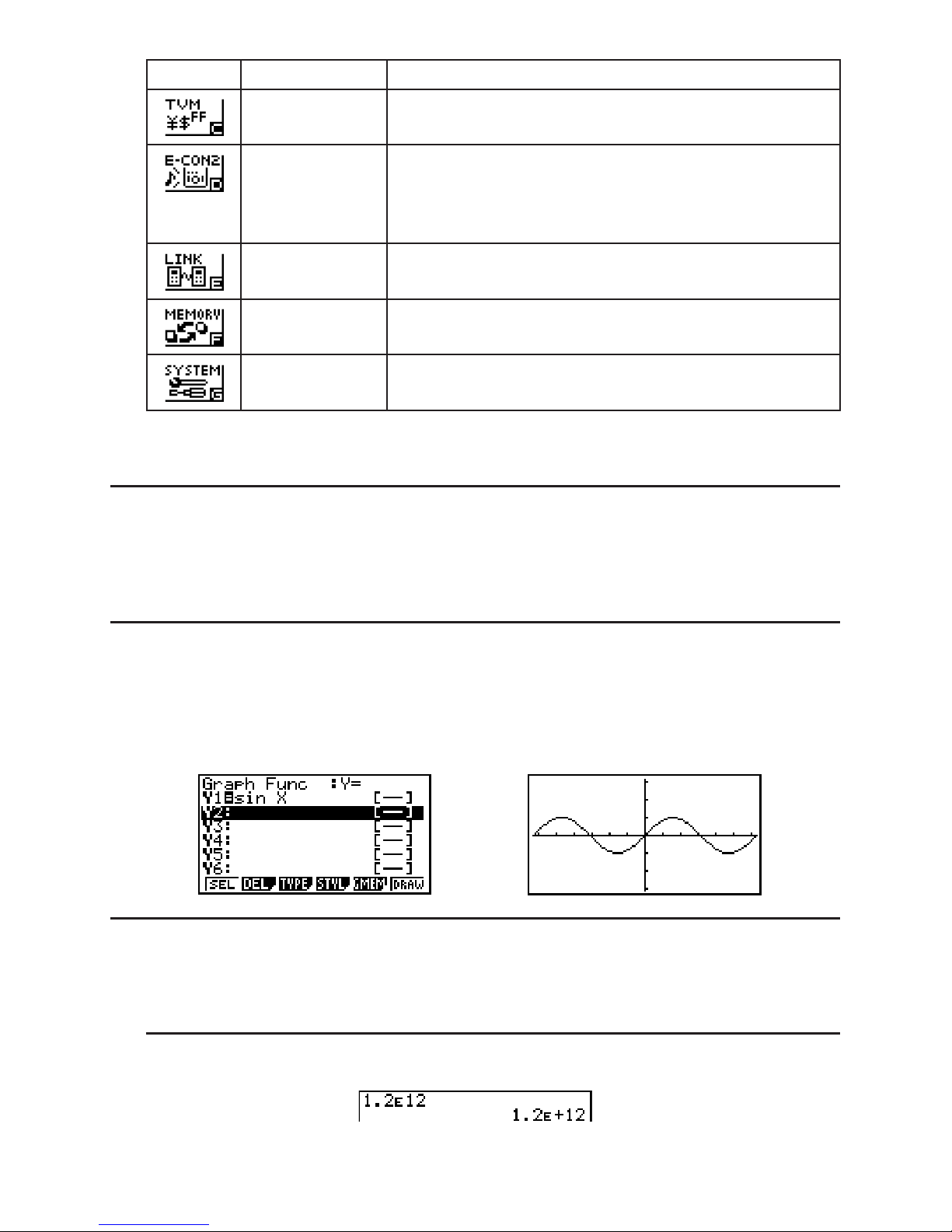
1.2E+12 indicates that the result is equivalent to 1.2 s 1012. This means that you should move

the decimal point in 1.2 twelve places to the right, because the exponent is positive. This results in the value 1,200,000,000,000.

1-5

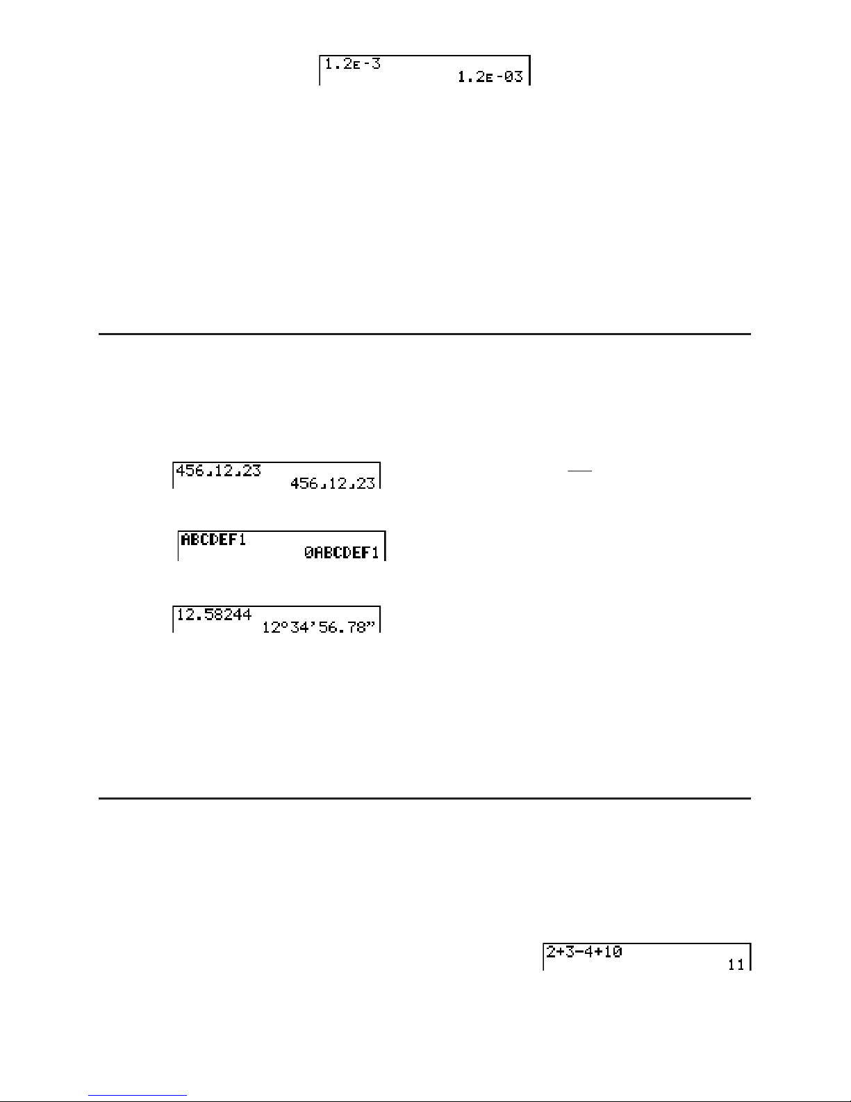
1.2E–03 indicates that the result is equivalent to 1.2 s 10–3. This means that you should move

the decimal point in 1.2 three places to the left, because the exponent is negative. This results in the value 0.0012.

You can specify one of two different ranges for automatic changeover to normal display.

Norm 1 ................... 10

–2

(0.01) > |x|, |x|  10

Norm 2 ................... 10–9 (0.000000001) > |x|, |x|  10

All of the examples in this manual show calculation results using Norm 1. See page 2-11 for details on switching between Norm 1 and Norm 2.

I Special Display Formats

This calculator uses special display formats to indicate fractions, hexadecimal values, and degrees/minutes/seconds values.

S Fractions

.................... Indicates: 456

12 23

S Hexadecimal Values

................... Indicates: 0ABCDEF1

(16)

, which equals

180150001

(10)

S Degrees/Minutes/Seconds

.................... Indicates: 12° 34’ 56.78”

• In addition to the above, this calculator also uses other indicators or symbols, which are

described in each applicable section of this manual as they come up.

3. Inputting and Editing Calculations

I Inputting Calculations

When you are ready to input a calculation, first press to clear the display. Next, input your calculation formulas exactly as they are written, from left to right, and press U to obtain the result.

Example 2 + 3 – 4 + 10 =

ABC@?U

1-6

I Editing Calculations

Use the B and C keys to move the cursor to the position you want to change, and then perform one of the operations described below. After you edit the calculation, you can execute it by pressing U. Or you can use C to move to the end of the calculation and input more.

• You can select either insert or overwrite for input*

. With overwrite, text you input replaces the text at the current cursor location. You can toggle between insert and overwrite by performing the operation: #(INS). The cursor appears as “I” for insert and as “ ” for overwrite.

With all models except the fx-7400Gɉ/fx-9750Gɉ, insert and overwrite switzng is possible only when the Linear input/output mode (page 1-29) is selected.

S To change a step

Example To change cos60 to sin60

AE?

BBB

S To delete a step

Example To change 369 ss 2 to 369 s 2

BEHA

In the insert mode, the # key operates as a backspace key.

S To insert a step

Example To change 2.362 to sin2.36

ABEV

BBBBB

1-7

I Using Replay Memory

The last calculation performed is always stored into replay memory. You can recall the contents of the replay memory by pressing B or C. If you press C, the calculation appears with the cursor at the beginning. Pressing B causes the calculation to appear with the cursor at the end. You can make changes in the calculation as you wish and then execute it again.

• Replay memory is enabled in the Linear input/output mode only. In the Math input/output mode, the history function is used in place of replay memory. For details, see “History Function” (page 1-17).

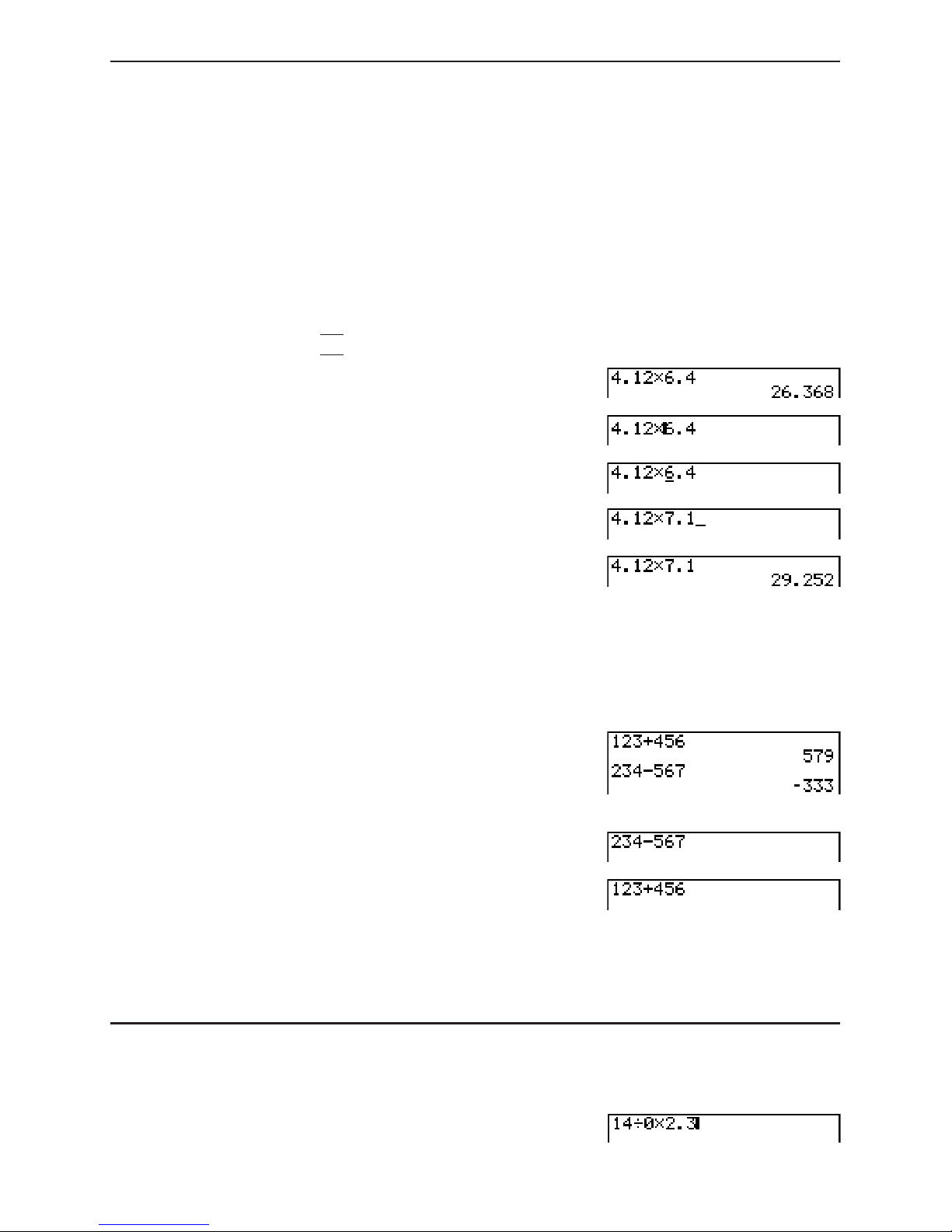
Example 1 To perform the following two calculations

4.12 s 6.4 = 26.368

4.12 s 7.1 = 29.252

C@AECU

BBBB

#(INS)

F@

After you press , you can press D or A to recall previous calculations, in sequence from the newest to the oldest (Multi-Replay Function). Once you recall a calculation, you can use C and B to move the cursor around the calculation and make changes in it to create a new calculation.

Example 2

@ABCDEU

ABCDEFU

D (One calculation back)

D (Two calculations back)

• A calculation remains stored in replay memory until you perform another calculation.

• The contents of replay memory are not cleared when you press the key, so you can recall a calculation and execute it even after pressing the key.

I Making Corrections in the Original Calculation

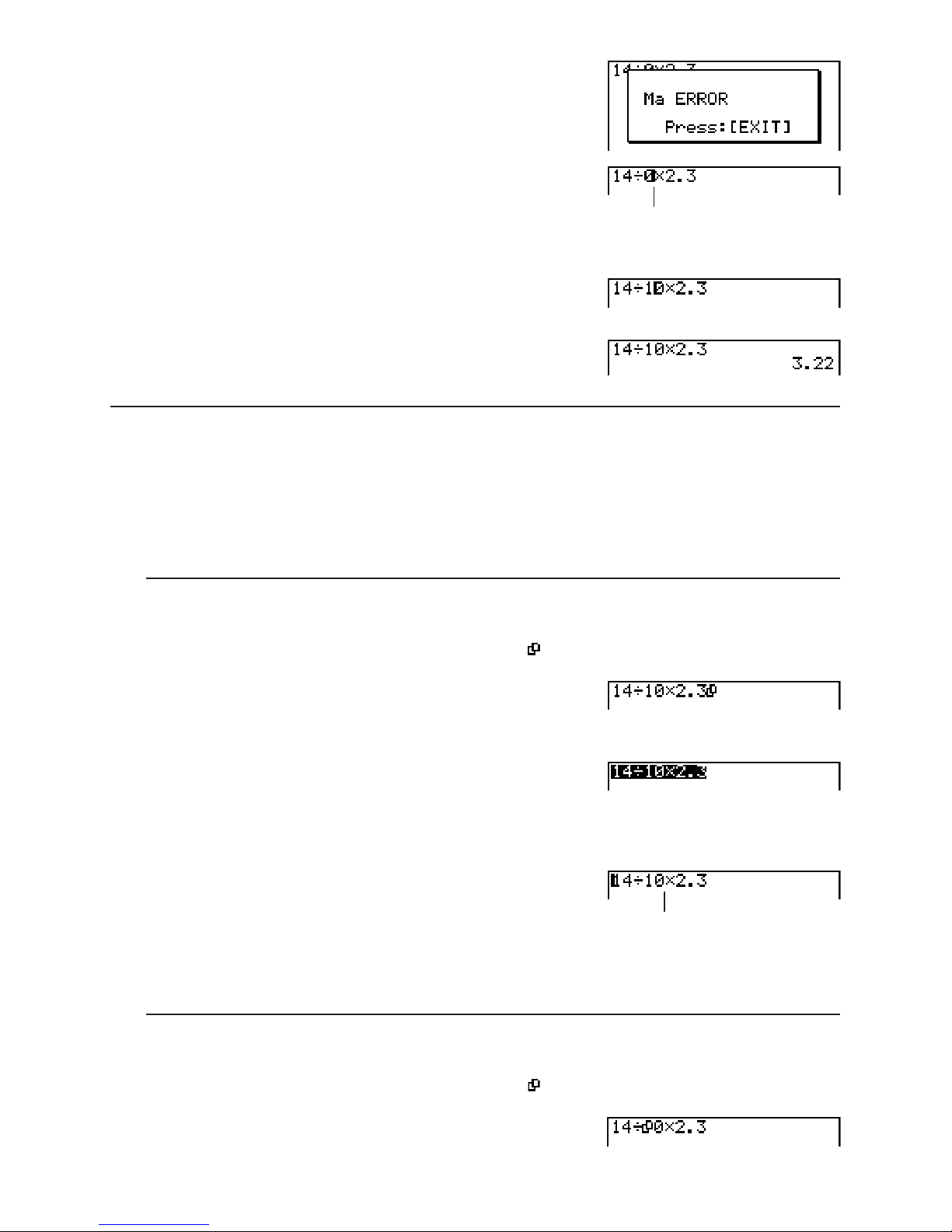
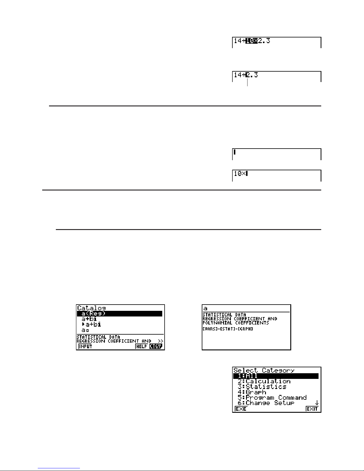
Example 14 w 0 s 2.3 entered by mistake for 14 w 10 s 2.3

@C?AB

1-8

Press ).

Cursor is positioned automatically at the location of the cause of the error.

Make necessary changes.

Execute again. U

I Using the Clipboard for Copy and Paste

You can copy (or cut) a function, command, or other input to the clipboard, and then paste the clipboard contents at another location.

• The procedures described here all use the Linear input/output mode. For details about the copy and paste operation while the Math input/output mode is selected, see “Using the Clipboard for Copy and Paste in the Math Input/Output Mode” (page 1-18).

S To specify the copy range

1. Move the cursor (I) to the beginning or end of the range of text you want to copy and then

press G(CLIP). This changes the cursor to “ ”.

2. Use the cursor keys to move the cursor and highlight the range of text you want to copy.

3. Press (COPY) to copy the highlighted text to the clipboard, and exit the copy range

specification mode.

The selected characters are not changed when you copy them.

To cancel text highlighting without performing a copy operation, press ).

S To cut the text

1. Move the cursor (I) to the beginning or end of the range of text you want to cut and then

press G(CLIP). This changes the cursor to “ ”.

1-9

2. Use the cursor keys to move the cursor and highlight the range of text you want to cut.

3. Press (CUT) to cut the highlighted text to the clipboard.

Cutting causes the original characters to be deleted.

S Pasting Text

Move the cursor to the location where you want to paste the text, and then press H(PASTE). The contents of the clipboard are pasted at the cursor position.

H(PASTE)

I Catalog Function

The Catalog is an alphabetic list of all the commands available on this calculator. You can input a command by calling up the Catalog and then selecting the command you want.

S To use the Catalog to input a command

1. Press C(CATALOG) to display an alphabetic Catalog of commands.

• The screen that appears first is the last one you used for command input.

• With the fx-9860G Slim, the first two lines of explanation text for the currently selected command will appear at the bottom of the screen. Pressing (HELP) will display a fullscreen view of the text for reading. If the text does not fit within a single screen, you can use D and A to scroll it.

(HELP)

m k

)

To close the help text screen, press ).

2. Press (CTGY) to display the category list.

• You can skip this step and go straight to step 5, if you want.

3. Use the cursor keys (D, A) to highlight the command category you want, and then press (EXE) or U.

• This displays a list of commands in the category you selected.

1-10

4. Input the first letter of the command you want to input. This will display the first command that starts with that letter.

5. Use the cursor keys (D, A) to highlight the command you want to input, and then press (INPUT) or U.

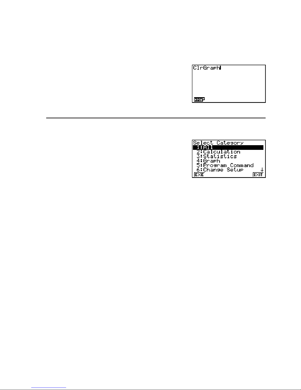
Example To use the Catalog to input the ClrGraph command

C(CATALOG)((C)A~AU

Pressing ) or )(QUIT) closes the Catalog.

S To input a command with ; (fx-9860G Slim only)

1. Press ;.

• This will display the category selection screen.

• (EXE)... {displays a list of commands in the currently selected category}

• (EXIT)... {exits the category selection screen}

2. Continue from step 3 of the procedure under “To use the Catalog to input a command”.

4. Using the Math Input/Output Mode

Important!

• The fx-7400G

ɉ and fx-9750Gɉ are not equipped with a Math input/output mode.

Selecting “Math” for the “Input/Output” mode setting on the Setup screen (page 1-29) turns on the Math input/output mode, which allows natural input and display of certain functions, just as they appear in your textbook.

• The operations in this section all are performed in the Math input/output mode.

- The initial default setting for the fx-9860G

ɉ SD/fx-9860Gɉ/fx-9860G AU PLUS is the Math

input/output mode. If you have changed to the Linear input/output mode, switch back to the Math input/output mode before performing the operations in this section. See “Using the Setup Screen” (page 1-26) for information about how to switch modes.

- The initial default setting for the fx-9860G Slim/fx-9860G SD/fx-9860G/fx-9860G AU is the Linear input/output mode. Switch to the Math input/output mode before performing the operations in this section. See “Using the Setup Screen” (page 1-26) for information about how to switch modes.

• In the Math input/output mode, all input is insert mode (not overwrite mode) input. Note that the #(INS) operation (page 1-6) you use in the Linear input/output mode to switch to insert mode input performs a completely different function in the Math input/output mode. For more information, see “Using Values and Expressions as Arguments” (page 1-14).

1-11

• Unless specifically stated otherwise, all operations in this section are performed in the RUN • MAT mode.

I Input Operations in the Math Input/Output Mode

S Math Input/Output Mode Functions and Symbols

The functions and symbols listed below can be used for natural input in the Math input/output mode. The “Bytes” column shows the number of bytes of memory that are used up by input in the Math input/output mode.

Function/Symbol Key Operation Bytes

Fraction (Improper)

Mixed Fraction*

6()

Power

Square

Negative Power (Reciprocal)

(

–1

)



V()

Cube Root

(

)

Power Root

,(

)

((ex)

J(10x)

log(a,b) (Input from MATH menu*

Abs (Absolute Value) (Input from MATH menu*

Linear Differential*

(Input from MATH menu*2)7

Quadratic Differential*Differential*

(Input from MATH menu*2)7

Integral*

(Input from MATH menu*2)8

3 Calculation*

(Input from MATH menu*2)11

Matrix (Input from MATH menu*

) 14*

Parentheses

 and 

Braces (Used during list input.)

( { ) and ( } )

Brackets (Used during matrix input.)

( [ ) and ( ] )

Mixed fraction is supported in the Math input/output mode only.

For information about function input from the MATH function menu, see “Using the MATH Menu” described below.

Tolerance cannot be specified in the Math input/output mode. If you want to specify tolerance, use the Linear input/output mode.

For 3 calculation in the Math input/output mode, the pitch is always 1. If you want to specify a different pitch, use the Linear input/output mode.

This is the number of bytes for a 2 × 2 matrix.

1-12

S Using the MATH Menu

In the RUN • MAT mode, pressing (MATH) displays the MATH menu. You can use this menu for natural input of matrices, differentials, integrals, etc.

•{MAT} ... {displays the MAT submenu, for natural input of matrices}

•{2s2} ... {inputs a 2 × 2 matrix}

•{3s3} ... {inputs a 3 × 3 matrix}

•{

msn} ... {inputs a matrix with m lines and n columns (up to 6 × 6)}

•{log

b} ... {starts natural input of logarithm logab}

•{Abs} ... {starts natural input of absolute value |X|}

•{

d/dx} ... {starts natural input of linear differential

(x)

}

•{

/dx2} ... {starts natural input of quadratic differential

f(x

)

}

•{°

dx} … {starts natural input of integral

f(x)dx

}

•{3(} … {starts natural input of 3 calculation

f(x

)

x=A

}

S Math Input/Output Mode Input Examples

This section provides a number of different examples showing how the MATH function menu and other keys can be used during Math input/output mode natural input. Be sure to pay attention to the input cursor position as you input values and data.

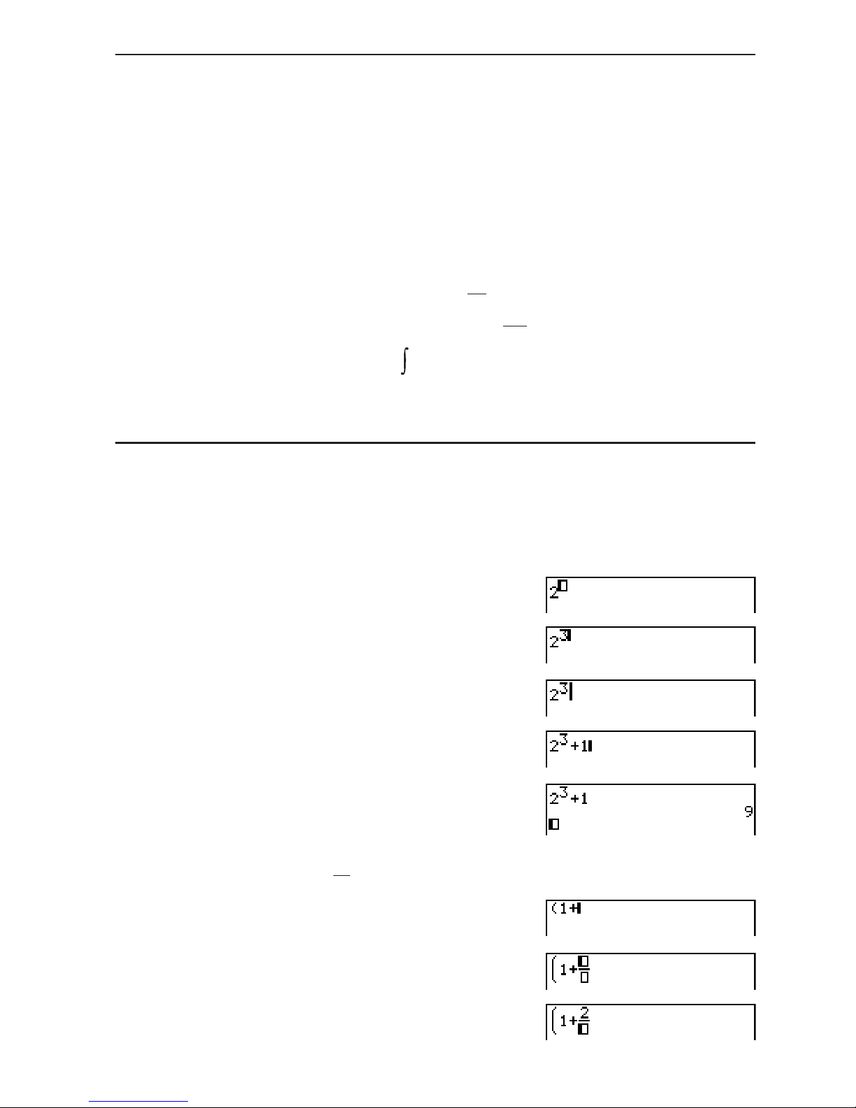
Example 1 To input 2

+ 1

@

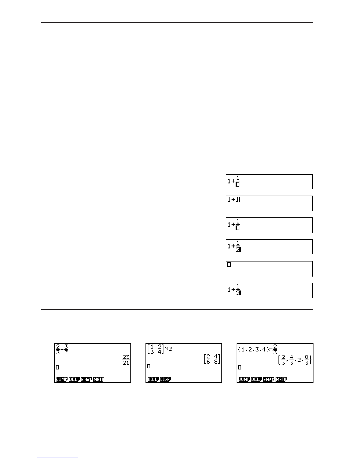
Example 2 To input

()

2 5

@

1-13

V

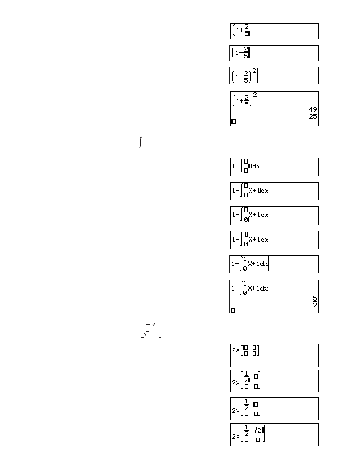
Example 3 To input

1+ x +1dx

@(MATH)(E)(

)

T@

Example 4 To input

2 ×

1 2

A(MATH)(MAT)(2×2)

6@AA

V()AC

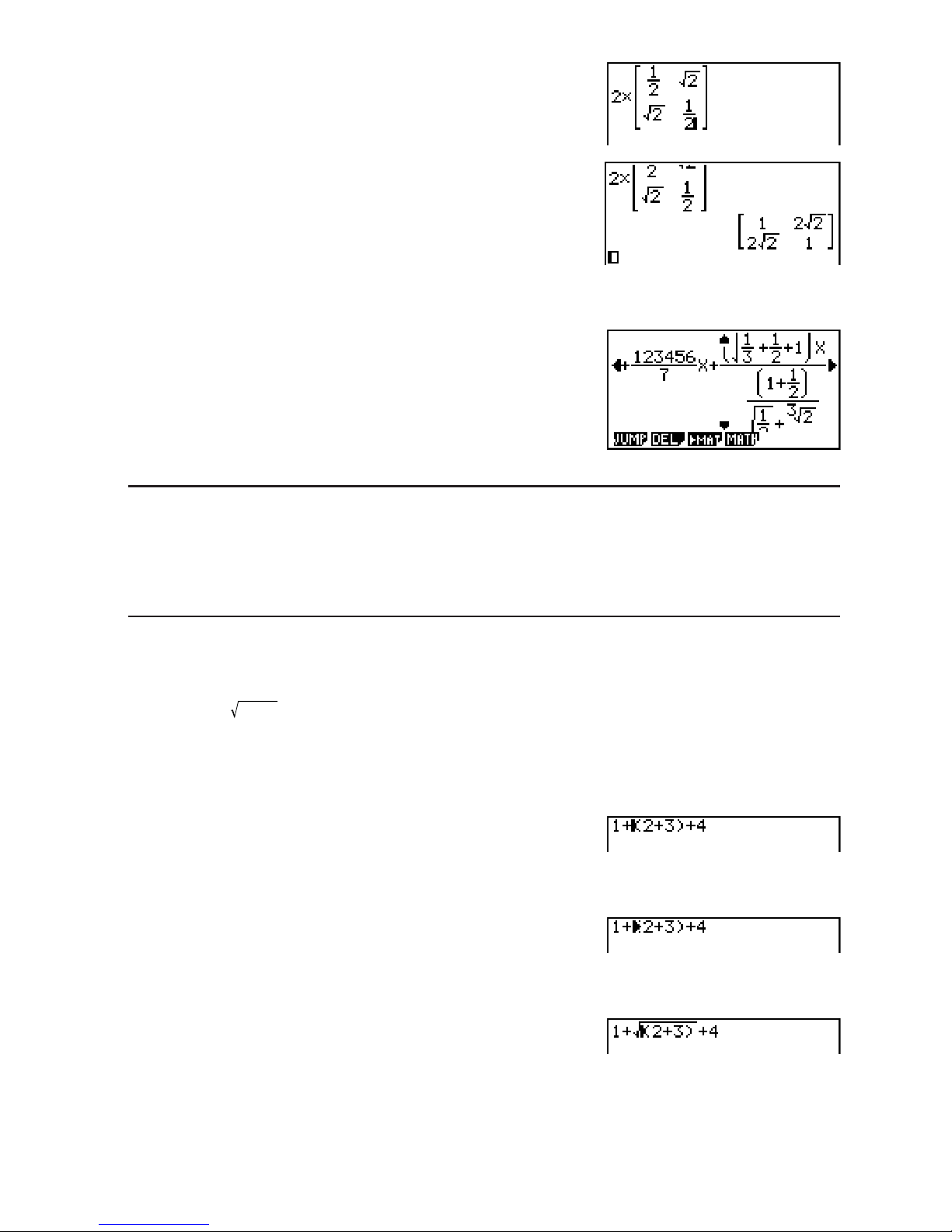
1-14

CV()ACC6@AA

S When the calculation does not fit within the display window

Arrows appear at the left, right, top, or bottom edge of the display to let you know when there is more of the calculation off the screen in the corresponding direction.

When you see an arrow, you can use the cursor keys to scroll the screen contents and view the part you want.

S Math Input/Output Mode Input Restrictions

Certain types of expressions can cause the vertical width of a calculation formula to be greater than one display line. The maximum allowable vertical width of a calculation formula is about two display screens (120 dots). You cannot input any expression that exceeds this limitation.

S Using Values and Expressions as Arguments

A value or an expression that you have already input can be used as the argument of a function. After you have input “(2+3)”, for example, you can make it the argument of , resulting in

(2+3)

Example

1. Move the cursor so it is located directly to the left of the part of the expression that you want

to become the argument of the function you will insert.

2. Press #(INS).

• This changes the cursor to an insert cursor ().

3. Press V() to insert the  function.

• This inserts the  function and makes the parenthetical expression its argument.

As shown above, the value or expression to the right of the cursor after #(INS) are pressed becomes the argument of the function that is specified next. The range encompassed as the argument is everything up to the first open parenthesis to the right, if there is one, or everything up to the first function to the right (sin(30), log2(4), etc.).

1-15

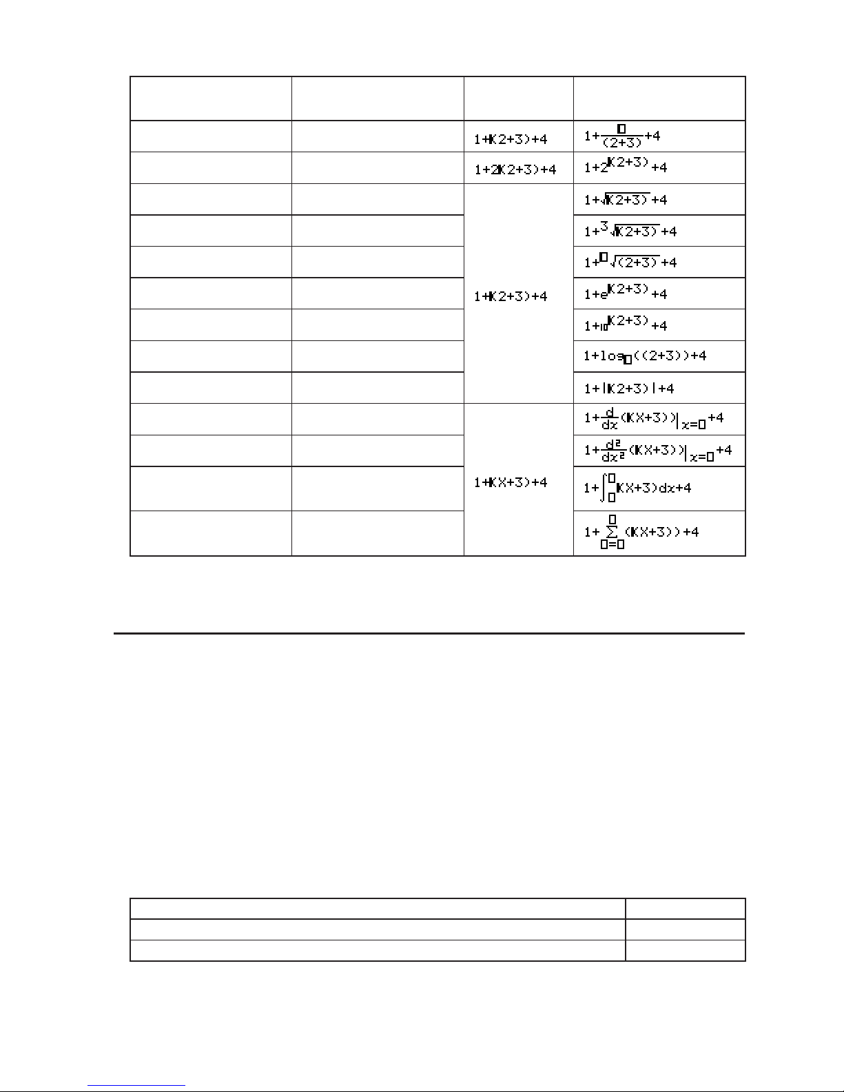
This capability can be used with the following functions.

Function Key Operation

Original

Expression

Expression After

Insertion

Improper Fraction

Power



V()

Cube Root

(

)

Power Root

,(

)

((ex)

J(10x)

log(a,b)

(MATH)(log

Absolute Value

(MATH)(Abs)

Linear Differential

(MATH)(

d/dx)

Quadratic Differential

(MATH)(

/dx2)

Integral

(MATH)(E) (°

dx)

3 Calculation

(MATH)(E) (3( )

• In the Linear input/output mode, pressing #(INS) will change to the insert mode. See page 1-6 for more information.

S Editing Calculations in the Math Input/Output Mode

The procedures for editing calculations in the Math input/output mode are basically the same as those for the Linear input/output mode. For more information, see “Editing Calculations” (page 1-6).

Note however, that the following points are different between the Math input/output mode and the Linear input/output mode.

• Overwrite mode input that is available in the Linear input/output mode is not supported by the Math input/output mode. In the Math input/output mode, input is always inserted at the current cursor location.

• In the Math input/output mode, pressing the # key always performs a backspace operation.

• Note the following cursor operations you can use while inputting a calculation with Math input/output mode.

To do this: Press this key:

Move the cursor from the end of the calculation to the beginning

Move the cursor from the beginning of the calculation to the end

1-16

I Using Undoing and Redoing Operations

You can use the following procedures during calculation expression input in the Math input/ output mode (up until you press the U key) to undo the last key operation and to redo the key operation you have just undone.

- To undo the last key operation, press: ?#(UNDO).

- To redo a key operation you have just undone, press: ?#(UNDO) again.

• You also can use UNDO to cancel an key operation. After pressing to clear an expression you have input, pressing ?#(UNDO) will restore what was on the display before you pressed .

• You also can use UNDO to cancel a cursor key operation. If you press C during input and then press ?#(UNDO), the cursor will return to where it was before you pressed C.

• The UNDO operation is disabled while the keyboard is alpha-locked. Pressing ?#(UNDO) while the keyboard is alpha-locked will perform the same delete operation as the # key alone.

Example

@6@C

?#(UNDO)

I Math Input/Output Mode Calculation Result Display

Fractions, matrices, and lists produced by Math input/output mode calculations are displayed in natural format, just as they appear in your textbook.

Sample Calculation Result Displays

• Fractions are displayed either as improper fractions or mixed fractions, depending on the “Frac Result” setting on the Setup screen. For details, see “Using the Setup Screen” (page 1-26).

1-17

• Matrices are displayed in natural format, up to 6 × 6. A matrix that has more than six rows or columns will be displayed on a MatAns screen, which is the same screen used in the Linear input/output mode.

• Lists are displayed in natural format for up to 20 elements. A list that has more than 20 elements will be displayed on a ListAns screen, which is the same screen used in the Linear input/output mode.

• Arrows appear at the left, right, top, or bottom edge of the display to let you know when there is more data off the screen in the corresponding direction.

You can use the cursor keys to scroll the screen and view the data you want.

• Pressing (DEL)(DEL

•

L) while a calculation result is selected will delete both the result

and the calculation that produced it.

• The multiplication sign cannot be omitted immediately before an improper fraction or mixed fraction. Be sure to always input a multiplication sign in this case.

Example:

2×

2 5

AA6D

•A,, V, or (

–1

) key operation cannot be followed immediately by another ,, V, or (x–1) key operation. In this case, use parentheses to keep the key operations separate.

Example: (3

2)–1

BV(x–1)

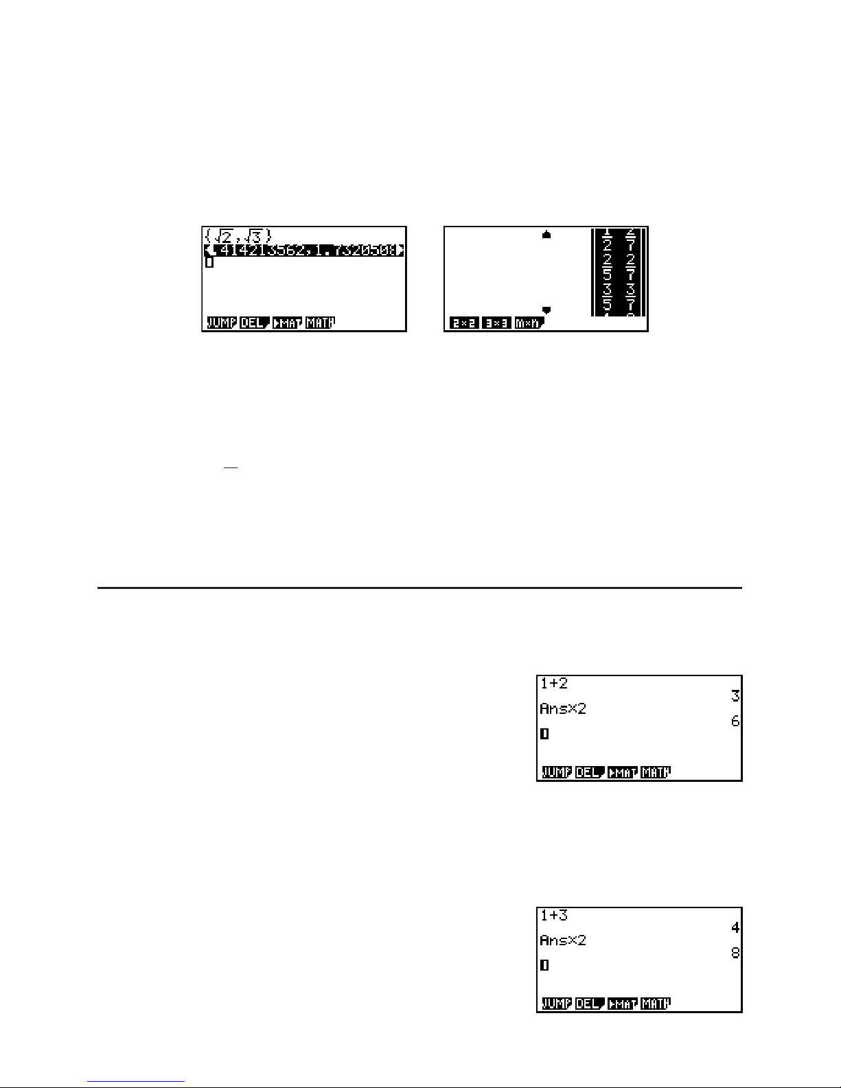
I History Function

The history function maintains a history of calculation expressions and results in the Math input/output mode. Up to 30 sets of calculation expressions and results are maintained.

@AU AU

You can also edit the calculation expressions that are maintained by the history function and recalculate. This will recalculate all of the expressions starting from the edited expression.

Example To change “1+2” to “1+3” and recalculate

Perform the following operation following the sample shown above.

DDDDB#BU

1-18

• The value stored in the answer memory is always dependent on the result produced by the last calculation performed. If history contents include operations that use the answer memory, editing a calculation may affect the answer memory value used in subsequent calculations.

- If you have a series of calculations that use the answer memory to include the result of the

previous calculation in the next calculation, editing a calculation will affect the results of all the other calculations that come after it.

- When the first calculation of the history includes the answer memory contents, the answer

memory value is “0” because there is no calculation before the first one in history.

I Using the Clipboard for Copy and Paste in the Math Input/Output Mode

You can copy a function, command, or other input to the clipboard, and then paste the clipboard contents at another location.

• In the Math input/output mode, you can specify only one line as the copy range.

• The CUT operation is supported for the Linear input/output mode only. It is not supported for the Math input/output mode.

S To copy text

1. Use the cursor keys to move the cursor to the line you want to copy.

2. Press G(CLIP). The cursor will change to “

”.

3. Press (CPY· L) to copy the highlighted text to the clipboard.

S To paste text

Move the cursor to the location where you want to paste the text, and then press

H(PASTE). The contents of the clipboard are pasted at the cursor position.

I Calculation Operations in the Math Input/Output Mode

This section introduces Math input/output mode calculation examples.

• For details about calculation operations, see “Chapter 2 Manual Calculations”.

S Performing Function Calculations Using Math Input/Output Mode

Example Operation

4×5610



( )

cos

(Angle: Rad)

6645U

A$(P)63CU

log

8 = 3

123 = 1.988647795

2 + 3 × 364 − 4 = 10

(MATH)(logab) 2C8U ,(

) 7C123U

23,(

) 3C64C4U

= 0.1249387366log

(MATH)(Abs)J364U

1-19

+ 3 =

1.5 + 2.3

265C36()1C4U

1.52.3?(

i)U,

( )

+x− 6

x = 3

= 52

(MATH)(d/dx)T,3C4

TVT6C3U

+ 3x + 4

404



(MATH)(E)(°dx) 2TV3T4C1 C5U

(

− 3k + 5) = 55

∑

(MATH)(E)(3)?(K)V3?(K) 5C?(K)C2C6U

I Performing Matrix Calculations Using Math Input/Output Mode

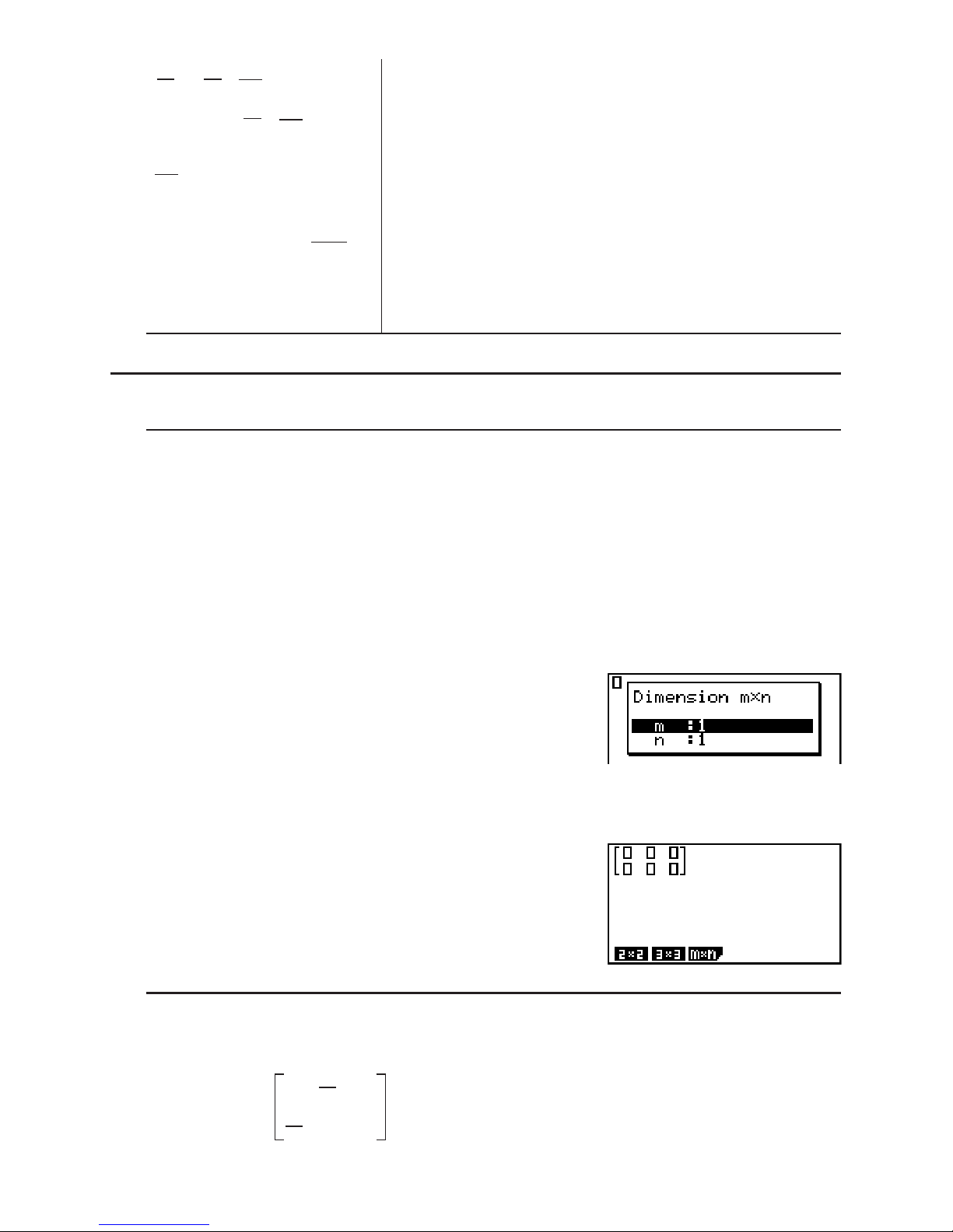
S To specify the dimensions (size) of a matrix

1. In the RUN• MAT mode, press K(SET UP)(Math)).

2. Press (MATH) to display the MATH menu.

3. Press (MAT) to display the following menu.

•{2s2} … {inputs a 2 × 2 matrix}

•{3s3} … {inputs a 3 × 3 matrix}

•{

msn} … {inputs an m-row × n-column matrix (up to 6 × 6)}

Example To create a 2-row s 3-column matrix

(

msn)

Specify the number of rows. AU Specify the number of columns. BU U

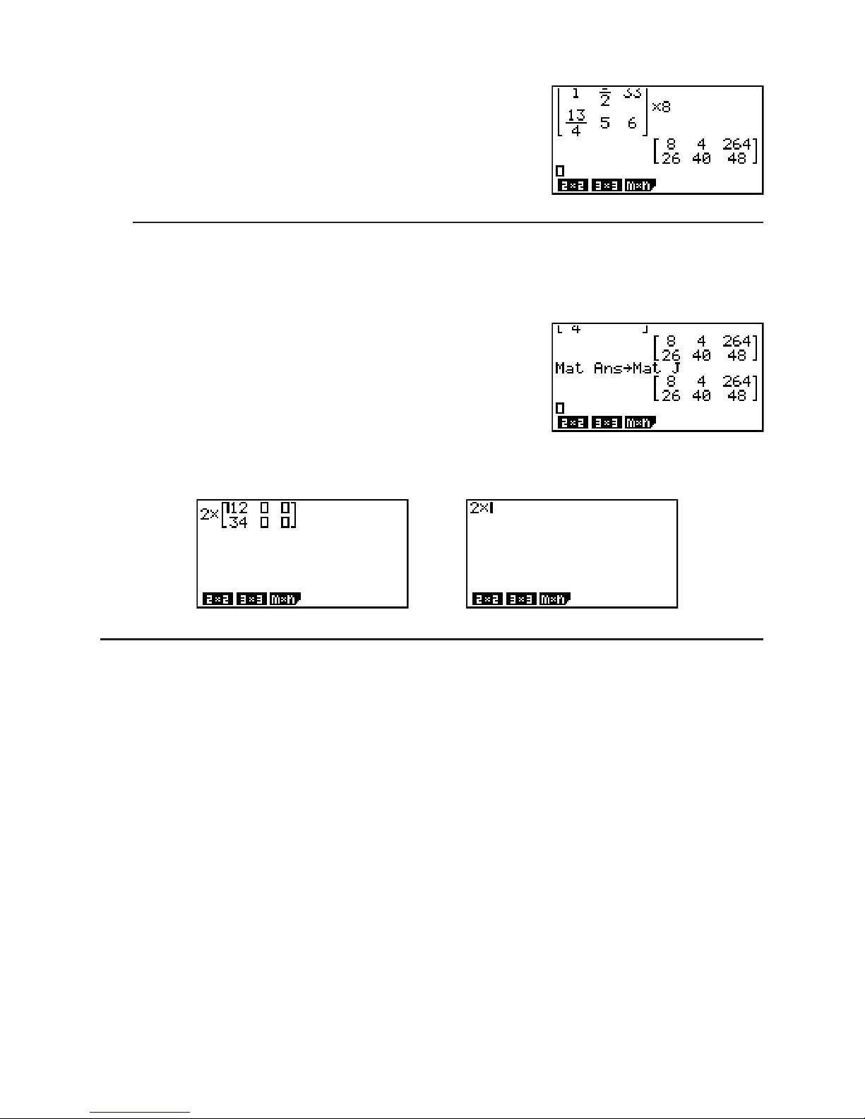
S To input cell values

Example To perform the calculation shown below

× 8

1 2

× 8

1 2

1-20

The following operation is a continuation of the example calculation on the previous page.

@C@6ACCBBC @B6CCCDCEC GU

S To assign a matrix created using Math input/output mode to a MAT mode

matrix

Example To assign the calculation result to Mat J

A(Mat)(Ans)?

A(Mat)?(J)U

• Pressing the # key while the cursor is located at the top (upper left) of the matrix will delete the entire matrix.



I Using Graph Modes and the EQUA Mode in the Math Input/Output

Mode

Using the Math input/output mode with any of the modes below lets you input numeric expressions just as they are written in your text book and view calculation results in natural display format.

Modes that support input of expressions as they are written in textbooks:

RUN • MAT, e • ACT, GRAPH, DYNA, TABLE, RECUR, EQUA (SOLV)

Modes that support natural display format:

RUN • MAT, e • ACT, EQUA

The following explanations show Math input/output mode operations in the GRAPH, DYNA, TABLE, RECUR and EQUA modes, and natural calculation result display in the EQUA mode.

• See the sections that cover each calculation for details about its operation.

• See “Input Operations in the Math Input/Output Mode” (page 1-11) and “Calculation Operations in the Math Input/Output Mode” (page 1-18) for details about Math input/output mode input operations and calculation result displays in the RUN • MAT mode.

• e • ACT mode input operations and result displays are the same as those in the RUN • MAT mode. For information about e • ACT mode operations, see “Chapter 10 eActivity”.

1-21

Important!

• On a model whose operating system has been updated to OS 2.00 from an older OS version, Math input/output mode input and result display are not supported in any mode except the RUN • MAT mode and e • ACT mode.

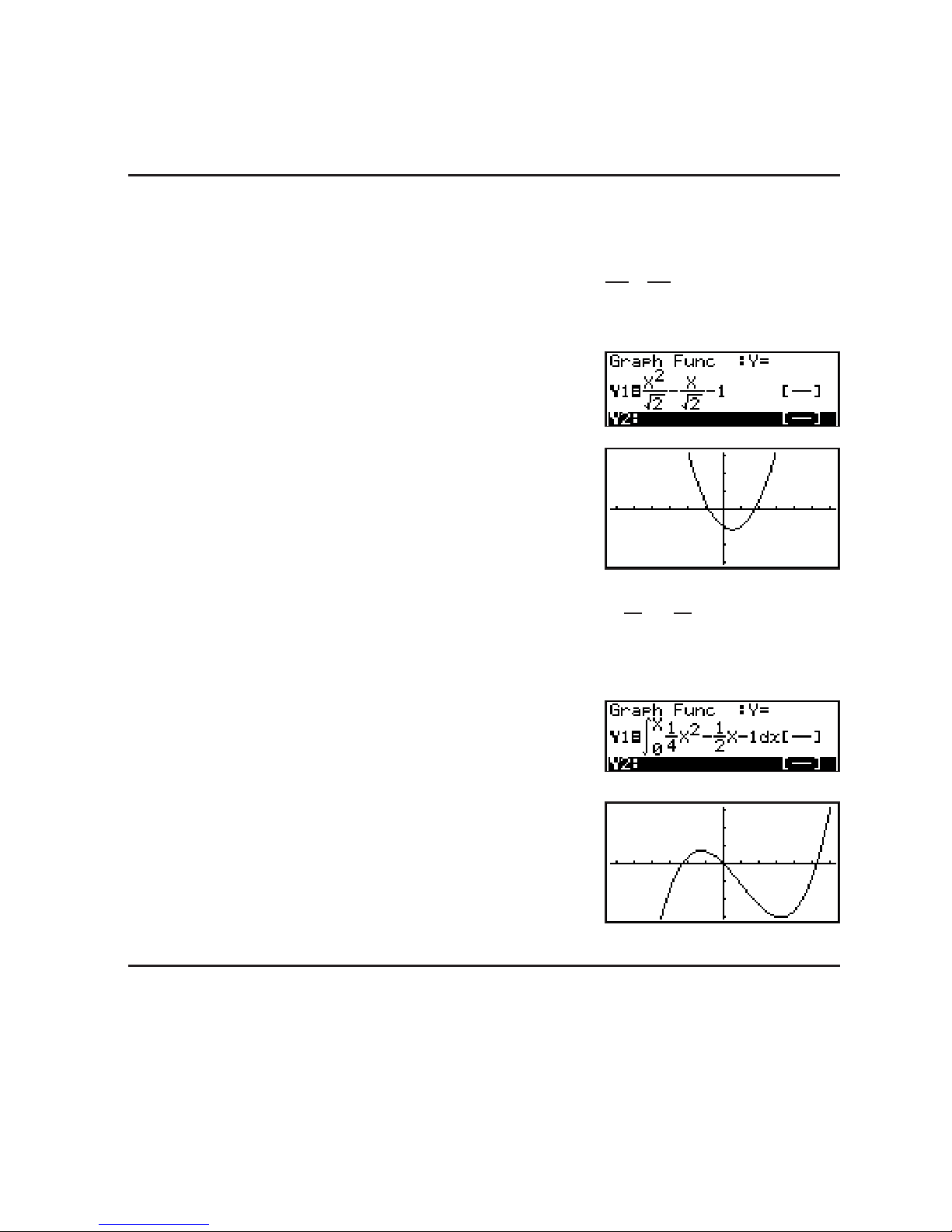
S Math Input/Output Mode Input in the GRAPH Mode

You can use the Math input/output mode for graph expression input in the GRAPH, DYNA, TABLE, and RECUR modes.

Example 1 In the GRAPH mode, input the function

−−1

and then graph it. Make sure that initial default settings are configured on the View Window.

KGRAPHTV6V()A\

CCT6V()ACC\

@U

(DRAW)

Example 2 In the GRAPH mode, input the function

−

x−1d



and then graph it. Make sure that initial default settings are configured on the View Window.

KGRAPH*(CALC)(°dx)

@6CCTV@6AC

T@C?CTU

(DRAW)

• Math Input/Output Mode Input and Result Display in the EQUA Mode

You can use the Math input/output mode in the EQUA mode for input and display as shown below.

• In the case of simultaneous equations ((SIML)) and high-order equations ((POLY)), solutions are output in natural display format (fractions, , P are displayed in natural format) whenever possible.

• In the case of Solver ((SOLV)), you can use Math input/output mode natural input.

1-22

Example To solve the quadratic equation

+ 3x + 5 = 0 in the EQUA mode

KEQUAK(SET UP) AAAA(Complex Mode)

(a+b

i))

(POLY)(2)@UBUDUU

5. Option (OPTN) Menu

The option menu gives you access to scientific functions and features that are not marked on the calculator’s keyboard. The contents of the option menu differ according to the mode you are in when you press the * key.

• The option menu does not appear if you press * while binary, octal, decimal, or hexadecimal is set as the default number system.

• For details about the commands included on the option (OPTN) menu, see the “* key” item in the “PRGM Mode Command List” (page 8-37).

• The meanings of the option menu items are described in the sections that cover each mode.

The following list shows the option menu that is displayed when the RUN • MAT (or RUN) or PRGM mode is selected.

Item names below that are marked with an asterisk (*) are not included on the fx-7400G

ɉ.

•{LIST} ... {list function menu}

•{MAT}* ... {matrix operation menu}

•{CPLX} ... {complex number calculation menu}

•{CALC} ... {functional analysis menu}

•{STAT} ... {paired-variable statistical estimated value menu} (fx-7400G

ɉ)

{menu for paired-variable statistical estimated value, distribution, standard deviation, variance, and test functions} (all models except fx-7400Gfx-7400Gɉ)

•{CONV} ... {metric conversion menu}

•{HYP} ... {hyperbolic calculation menu}

•{PROB} ... {probability/distribution calculation menu}

•{NUM} ... {numeric calculation menu}

•{ANGL} ... {menu for angle/coordinate conversion, sexagesimal input/conversion}

•{ESYM} ... {engineering symbol menu}

•{PICT} ... {graph save/recall menu}

•{FMEM} ... {function memory menu}

•{LOGIC} ... {logic operator menu}

•{CAPT} ... {screen capture menu}

•{TVM}* ... {financial calculation menu}

• The PICT, FMEM and CAPT items are not displayed when “Math” is selected for the “Input/ Output” mode setting on the Setup screen.

1-23

6. Variable Data (VARS) Menu

To recall variable data, press ) to display the variable data menu. {V-WIN}/{FACT}/{STAT}/{GRPH}/{DYNA}/{TABL}/{RECR}/{EQUA}/{TVM}/{Str}

• Note that the EQUA and TVM items appear for function keys ( and ) only when you access the variable data menu from the RUN • MAT (or RUN) or PRGM mode.

• The variable data menu does not appear if you press ) while binary, octal, decimal, or hexadecimal is set as the default number system.

• Depending on the calculator model, some menu items may not be included.

• For details about the commands included on the variable data (VARS) menu, see the “) key” item in the “PRGM Mode Command List” (page 8-37).

• Item names below that are marked with an asterisk (*) are not included on the fx-7400G

ɉ.

S V-WIN — Recalling V-Window values

• {X}/{Y}/{T,Ƨ} ... {x-axis menu}/{y-axis menu}/{T,Ƨmenu}

•

{R-X}/{R-Y}/{R-T,Ƨ} ... {x-axis menu}/{y-axis menu}/{T,Ƨmenu} for right side of Dual

Graph

•{min}/{max}/{scal}/{dot}/{ptch} ... {minimum value}/{maximum value}/{scale}/{dot value*

}/{pitch}

The dot value indicates the display range (Xmax value – Xmin value) divided by the

screen dot pitch (126). The dot value is normally calculated automatically from the minimum and maximum values. Changing the dot value causes the maximum to be calculated automatically.

S FACT — Recalling zoom factors

• {Xfct}/{Yfct} ... {x-axis factor}/{y-axis factor}

S STAT — Recalling statistical data

•{X} … {single-variable, paired-variable x-data}

• {

n}/{¯x}/{3x}/{3x

}/{Ʊx}/{sx}/{minX}/{maxX} ... {number of data}/{mean}/{sum}/{sum of squares}/{population standard deviation}/{sample standard deviation}/{minimum value}/{maximum value}

•

{Y} ... {paired-variable y-data}

• {

Κ}/{3y}/{3y

}/{3xy}/{Ʊx}/{sy}/{minY}/{maxY} ... {mean}/{sum}/{sum of squares}/{sum of products of x-data and y-data}/{population standard deviation}/{sample standard deviation}/{minimum value}/{maximum value}

•

{GRPH} ... {graph data menu}

• {a}/{b}/{c}/{d}/{e} ... {regression coefficient and polynomial coefficients}

• {r}/{r

} ... {correlation coefficient}/{coefficient of determination}

• {MSe} ... {mean square error}

• {Q

}/{Q3} ... {first quartile}/{third quartile}

• {Med}/{Mod} ... {median}/{mode} of input data

• {Strt}/{Pitch} ... histogram {start division}/{pitch}

•

{PTS} ... {summary point data menu}

• {

}/{y1}/{x2}/{y2}/{x3}/{y3} ... {coordinates of summary points}

1-24

•

{INPT}* ... {statistical calculation input values}

• {n}/{¯x}/{sx}/{n1}/{n2}/{¯x1}/{¯x2}/{s

}/{s

}/{sp} ... {size of sample}/{mean of sample}/{sample standard deviation}/{size of sample 1}/{size of sample 2}/{mean of sample 1}/{mean of sample 2}/{standard deviation of sample 1}/{standard deviation of sample 2}/{standard deviation of sample p}

•

{RESLT}* ... {statistical calculation output values}

• {TEST} ... {test calculation results}

• {

p}/{z}/{t}/{Chi}/{F}/{ˆp}/{ ˆp

}/{ˆp2}/{df}/{se}/{r}/{r2}/{pa}/{Fa}/{Adf}/{SSa}/{MSa}/{pb}/{Fb}/

{Bdf}/{SSb}/{MSb}/{pab}/{Fab}/{ABdf}/{SSab}/{MSab}/{Edf}/{SSe}/{MSe}

... {p-value}/{z score}/{t score}/{C2 value}/{F value}/{estimated sample proportion}/ {estimated proportion of sample 1}/{estimated proportion of sample 2}/{degrees of freedom}/{standard error}/{correlation coefficient}/{coefficient of determination}/ {factor A p-value}/{factor A F value}/{factor A degrees of freedom}/{factor A sum of squares}/{factor A mean squares}/{factor B p-value}/{factor B F value}/{factor B degrees of freedom}/{factor B sum of squares}/ {factor B mean squares}/{factor AB p-value}/{factor AB F value}/{factor AB degrees of freedom}/{factor AB sum of squares}/{factor AB mean squares}/{error degrees of freedom}/{error sum of squares}/{error mean squares}

• {INTR} ... {confidence interval calculation results}

• {Left}/{Right}/{

ˆp}/{ ˆp

}/{ˆp2}/{df} ... {confidence interval lower limit (left edge)}/ {confidence interval upper limit (right edge)}/{estimated sample proportion}/ {estimated proportion of sample 1}/{estimated proportion of sample 2}/{degrees of freedom}

• {DIST} ... {distribution calculation results}

• {

p}/{xInv}/{x1Inv}/{x2Inv}/{zLow}/{zUp}/{tLow}/{tUp} ... {probability distribution

or cumulative distribution calculation result (p-value)}/{inverse Student-t, C2, F, binomial, Poisson, geometric or hypergeometric cumulative distribution calculation result}/{inverse normal cumulative distribution upper limit (right edge) or lower limit (left edge)}/{inverse normal cumulative distribution upper limit (right edge)}/{normal cumulative distribution lower limit (left edge)}/{normal cumulative distribution upper limit (right edge)}/{Student-t cumulative distribution lower limit (left edge)}/{Student-t cumulative distribution upper limit (right edge)}

S GRPH — Recalling graph functions

•{Y}/{r} ... {rectangular coordinate or inequality function}/{polar coordinate function}

•{Xt}/{Yt} ... parametric graph function {Xt}/{Yt}

•{X} ... {X=constant graph function}

• Press these keys before inputting a value to specify a memory area.

S DYNA* — Recalling dynamic graph setup data

•{Strt}/{End}/{Pitch} ... {coefficient range start value}/{coefficient range end value}/ {coefficient value increment}

S TABL — Recalling table setup and content data

•{Strt}/{End}/{Pitch} ... {table range start value}/{table range end value}/{table value increment}

•{Reslt*

} ... {matrix of table contents}

The Reslt item appears only when the TABL menu is displayed in the RUN • MAT (or RUN) and PRGM modes.

1-25

S RECR* — Recalling recursion formula*1, table range, and table content data

•{FORM} ... {recursion formula data menu}

• {an}/{a

}/{a

}/{bn}/{b

}/{b

}/{cn}/{c

}/{c

} ... {an}/{a

}/{a

}/{bn}/{b

}/{b

}/{cn}/

}/{c

} expressions

•{RANG} ... {table range data menu}

• {Strt}/{End} ... table range {start value}/{end value}

• {

}/{a1}/{a2}/{b0}/{b1}/{b2}/{c0}/{c1}/{c2} ... {a0}/{a1}/{a2}/{b0}/{b1}/{b2}/{c0}/{c1}/{c2} value

• {

St}/{bnSt}/{cnSt} ... origin of {an}/{bn}/{cn} recursion formula convergence/divergence

graph (WEB graph)

•{Reslt*

}* ... {matrix of table contents*3}

An error occurs when there is no function or recursion formula numeric table in memory.

“Reslt” is available only in the RUN • MAT and PRGM modes.

Table contents are stored automatically in Matrix Answer Memory (MatAns).

S EQUA* — Recalling equation coefficients and solutions*1 *

•{S-Rlt}/{S-Cof} ... matrix of {solutions}/{coefficients} for linear equations with two through six unknowns*

•{P-Rlt}/{P-Cof} ... matrix of {solution}/{coefficients} for a quadratic or cubic equation *

Coefficients and solutions are stored automatically in Matrix Answer Memory (MatAns).

The following conditions cause an error.

- When there are no coefficients input for the equation

- When there are no solutions obtained for the equation

Coefficient and solution memory data for a linear equation cannot be recalled at the same time.

S TVM* — Recalling financial calculation data

•{n}/{I%}/{PV}/{PMT}/{FV} ... {payment periods (installments)}/{annual interest rate}/ {present value}/{payment}/{future value}

•{

P/Y}/{C/Y} ... {installment periods per year}/{compounding periods per year}

S Str — Str command

•{Str} ... {string memory}

7. Program (PRGM) Menu

To display the program (PRGM) menu, first enter the RUN • MAT (or RUN) or PRGM mode from the Main Menu and then press )(PRGM). The following are the selections available in the program (PRGM) menu.

•{COM} ...... {program command menu}

•{CTL} ....... {program control command menu}

•{JUMP}..... {jump command menu}

•{?} ............ {input command}

•{<} .......... {output command}

•{CLR} ....... {clear command menu}

1-26

•{DISP} ...... {display command menu}

•{REL} ....... {conditional jump relational operator menu}

•{I/O} ......... {I/O control/transfer command menu}

•{:} ............. {multi-statement command}

•{STR} ....... {string command}

The following function key menu appears if you press )(PRGM) in the RUN • MAT (or RUN) mode or the PRGM mode while binary, octal, decimal, or hexadecimal is set as the default number system.

•{Prog}....... {program recall}

•{JUMP}/{?}/{<}/{REL}/{:}

The functions assigned to the function keys are the same as those in the Comp mode. For details on the commands that are available in the various menus you can access from the

program menu, see “Chapter 8 Programming”.

8. Using the Setup Screen

The mode’s Setup screen shows the current status of mode settings and lets you make any changes you want. The following procedure shows how to change a setup.

S To change a mode setup

1. Select the icon you want and press U to enter a mode and display its initial screen. Here

we will enter the RUN • MAT (or RUN) mode.

2. Press K(SET UP) to display the mode’s Setup

screen.

• This Setup screen is just one possible example. Actual Setup screen contents will differ according to the mode you are in and that mode’s current settings.

3. Use the D and A cursor keys to move the highlighting to the item whose setting you

want to change.

4. Press the function key ( to ) that is marked with the setting you want to make.

5. After you are finished making any changes you want, press ) to exit the Setup screen.

I Setup Screen Function Key Menus

This section details the settings you can make using the function keys in the Setup screen.

indicates default setting.

Item names below that are marked with an asterisk (*) are not included on the fx-7400G

ɉ.

1-27

S Mode (calculation/binary, octal, decimal, hexadecimal mode)

•{Comp} ... {arithmetic calculation mode}

•{Dec}/{Hex}/{Bin}/{Oct} ... {decimal}/{hexadecimal}/{binary}/{octal}

S Frac Result (fraction result display format)

•{d/c}/{ab/c} ... {improper}/{mixed} fraction

S Func Type (graph function type)

Pressing one of the following function keys also switches the function of the T key.

•{Y=}/{r=}/{Parm}/{X=} ... {rectangular coordinate (Y=

I(x) type)}/{polar coordinate}/

{parametric}/{rectangular coordinate (X=

I(y) type)} graph

•{Y>}/{Y<}/{YP}/{YO} ... {

y>f(x)}/{y<f(x)}/{yrf(x)}/{ybf(x)} inequality graph

•{X>}/{X<}/{XP}/{XO} ... {

x>f(y)}/{x<f(y)}/{xrf(y)}/{xbf(y)} inequality graph

S Draw Type (graph drawing method)

•{Con}/{Plot} ... {connected points}/{unconnected points}... {connected points}/{unconnected points}

S Derivative (derivative value display)

•{On}/{Off} ... {display on}/{display off} while Graph-to-Table, Table & Graph, and Trace are being used

S Angle (default angle unit)

•{Deg}/{Rad}/{Gra} ... {degrees}/{radians}/{grads}

S Complex Mode

•{Real} ... {calculation in real number range only}

•{

a+bi}/{rƧ} ... {rectangular format}/{polar format} display of a complex calculation

S Coord (graph pointer coordinate display)

•{On}/{Off} ... {display on}/{display off}

S Grid (graph gridline display)

•{On}/{Off} ... {display on}/{display off}

S Axes (graph axis display)

•{On}/{Off} ... {display on}/{display off}

S Label (graph axis label display)

•{On}/{Off} ... {display on}/{display off}

S Display (display format)

•{Fix}/{Sci}/{Norm}/{Eng} ... {fixed number of decimal places specification}/{number of significant digits specification}/{normal display setting}/{engineering mode}

S Stat Wind (statistical graph V-Window setting method)

•{Auto}/{Man} ... {automatic}/{manual}

S Resid List (residual calculation)

•{None}/{LIST} ... {no calculation}/{list specification for the calculated residual data}

1-28

S List File (list file display settings)

•{FILE} ... {settings of list file on the display}

S Sub Name (list naming)

•{On}/{Off} ... {display on}/{display off}

S Graph Func (function display during graph drawing and trace)

•{On}/{Off} ... {display on}/{display off}

S Dual Screen (dual screen mode status)

•{G+G}/{GtoT}/{Off} ... {graphing on both sides of dual screen}/{graph on one side and numeric table on the other side of dual screen}/{dual screen off}

S Simul Graph (simultaneous graphing mode)

•{On}/{Off} ... {simultaneous graphing on (all graphs drawn simultaneously)}/{simultaneous graphing off (graphs drawn in area numeric sequence)}

S Background (graph display background)

•{None}/{PICT} ... {no background}/{graph background picture specification}

S Sketch Line (overlaid line type)

•{ }/{ }/{ }/{ } ... {normal}/{thick}/{broken}/{dotted}

S Dynamic Type* (dynamic graph type)

•{Cnt}/{Stop} ... {non-stop (continuous)}/{automatic stop after 10 draws}

S Locus* (dynamic graph locus mode)

•{On}/{Off} ... {locus drawn}/{locus not drawn}

S Y=Draw Speed* (dynamic graph draw speed)

•{Norm}/{High} ... {normal}/{high-speed}

S Variable (table generation and graph draw settings)

•{RANG}/{LIST} ... {use table range}/{use list data}

S 3 Display* (3 value display in recursion table)

•{On}/{Off} ... {display on}/{display off}

S Slope* (display of derivative at current pointer location in conic section

graph)

•{On}/{Off} ... {display on}/{display off}

S Payment* (payment period setting)

•{BGN}/{END} ... {beginning}/{end} setting of payment period

S Date Mode* (number of days per year setting)

•{365}/{360} ... interest calculations using {365}*1/{360} days per year

The 365-day year must be used for date calculations in the TVM mode. Otherwise, an

error occurs.

1-29

S Periods/YR. * (payment interval specification)

•{Annu}/{Semi} ... {annual}/{semiannual}

S Ineq Type (inequality fill specification)

•{AND}/{OR} ... When graphing multiple inequalities, {fill areas where all inequality conditions are satisfied}/{fill areas where each inequality condition is satisfied}

S Simplify (calculation result auto/manual reduction specification)

•{Auto}/{Man} ... {auto reduce and display}/{display without reduction}

S Q1Q3 Type (Q1/Q3 calculation formulas)

•{Std}/{OnData} ... {Divide total population on its center point between upper and lower groups, with the median of the lower group Q1 and the median of the upper group Q3}/ {Make the value of element whose cumulative frequency ratio is greater than 1/4 and nearest to 1/4 Q1 and the value of element whose cumulative frequency ratio is greater than 3/4 and nearest to 3/4 Q3}

The following items are not included on the fx-7400G

ɉ/fx-9750Gɉ.

S Input/Output (input/output mode)

•{Math}/{Line}*1 ... {Math}/{Linear} input/output mode

S Auto Calc (spreadsheet auto calc)

•{On}/{Off} ... {execute}/{not execute} the formulas automatically

S Show Cell (spreadsheet cell display mode)

•{Form}/{Val} ... {formula}*2/{value}

S Move (spreadsheet cell cursor direction)*

•{Low}/{Right} ... {move down}/{move right}

The initial default setting of the fx-9860G Slim (OS 2.00)/fx-9860G SD (OS 2.00)/fx-

9860G (OS 2.00)/fx-9860G AU (OS 2.00) is the “Line” input/output mode.

Selecting “Form” (formula) causes a formula in the cell to be displayed as a formula. The

“Form” does not affect any non-formula data in the cell.

Specifies the direction the cell cursor moves when you press the U key to register cell

input, when the Sequence command generates a number table, and when you recall data from List memory.

9. Using Screen Capture

Any time while operating the calculator, you can capture an image of the current screen and save it in capture memory.

S To capture a screen image

1. Operate the calculator and display the screen you want to capture.

1-30

2. Press F(CAPTURE).

• This displays a memory area selection dialog box.

3. Input a value from 1 to 20 and then press U.

• This will capture the screen image and save it in capture memory area named “Capt

n”

(n = the value you input).

• You cannot capture the screen image of a message indicating that an operation or data

communication is in progress.

• A memory error will occur if there is not enough room in main memory to store the screen

capture.

S To recall a screen image from capture memory

This operation is possible only while the Linear input/output mode is selected.

1. In the RUN• MAT (or RUN) mode, press *(E)

(E)(CAPT)((CAPT) on the fx-7400G

ɉ)

(RCL).

2. Enter a capture memory number in the range of 1 to 20, and then press U.

• This displays the image stored in the capture memory you specified.

3. To exit the image display and return to the screen you started from in step 1, press ).

• You can also use the RclCapt command in a program to recall a screen image from capture

memory.

10. When you keep having problems…

If you keep having problems when you are trying to perform operations, try the following before assuming that there is something wrong with the calculator.

I Getting the Calculator Back to its Original Mode Settings

1. From the Main Menu, enter the SYSTEM mode.

2. Press (RSET).

3. Press (STUP), and then press (Yes).

4. Press )K to return to the Main Menu. Now enter the correct mode and perform your calculation again, monitoring the results on the

display.

1-31

I Restart and Reset

S Restart

Should the calculator start to act abnormally, you can restart it by pressing the RESTART button (P button). Note, however, that you should only use the RESTART button only as a last resort. Normally, pressing the RESTART button reboots the calculator’s operating system, so programs, graph functions and other data in calculator memory is retained.

Important!

The calculator backs up user data (main memory) when you turn power off and loads the backed up data when you turn power back on.

When you press the RESTART button, the calculator restarts and loads backed up data. This means that if you press the RESTART button after you edit a program, graph function, or other data, any data that has not been backed up will be lost.

S Reset

Use reset when you want to delete all data currently in calculator memory and return all mode settings to their initial defaults.

Before performing the reset operation, first make a written copy of all important data. For details, see “Reset” (page 12-3).

I Low Battery Message

If the following message appears on the display, immediately turn off the calculator and replace batteries as instructed.

If you continue using the calculator without replacing batteries, power will automatically turn off to protect memory contents. Once this happens, you will not be able to turn power back on, and there is the danger that memory contents will be corrupted or lost entirely.

• You will not be able to perform data communications operations after the low battery

message appears.

fx-9860G SD fx-9860G fx-9860G AU PLUS

fx-9750G fx-7400G

fx-9860G SD fx-9860G

fx-9860G Slim

RESTART button

P button

fx-9860G SD fx-9860G fx-9860G AU PLUS

fx-9750G fx-7400G

fx-9860G SD fx-9860G

fx-9860G Slim

RESTART button

P button

2-1

Chapter 2 Manual Calculations

1. Basic Calculations

I Arithmetic Calculations

• Enter arithmetic calculations as they are written, from left to right.

• Use the  key to input the minus sign before a negative value.

• Calculations are performed internally with a 15-digit mantissa. The result is rounded to a 10-

digit mantissa before it is displayed.

• For mixed arithmetic calculations, multiplication and division are given priority over addition

and subtraction.

Example Operation

56 × (–12) ÷ (–2.5) = 268.8

56122.5U

(2+3)× 10

= 500

231$2U

2+3×(4+5)=29

2345U*

4×5

= 0.3

645U

Final closed parentheses (immediately before operation of the U key) may be omitted, no matter how many are required.

I Number of Decimal Places, Number of Significant Digits, Normal

Display Range

[SET UP]-[Display]-[Fix] / [Sci] / [Norm]

• Even after you specify the number of decimal places or the number of significant digits,

internal calculations are still performed using a 15-digit mantissa, and displayed values are stored with a 10-digit mantissa. Use Rnd of the Numeric Calculation Menu (NUM) (page 2-12) to round the displayed value off to the number of decimal place and significant digit settings.

• Number of decimal place (Fix) and significant digit (Sci) settings normally remain in effect

until you change them or until you change the normal display range (Norm) setting.

Example 1 100 w 6 = 16.66666666...

Condition Operation Display

1006U

16.66666667

4 decimal places

K(SET UP) DD

(Fix)CU)U

16.6667

5 significant digits

K(SET UP) DD

(Sci)DU)U

1.6667E+01

Cancels specification

K(SET UP) DD

(Norm))U

16.66666667

Displayed values are rounded off to the place you specify.

*1*

2-2

Example 2 200 w 7 s 14 = 400

Condition Operation Display

200714U

400

3 decimal places

K(SET UP) DD

(Fix)BU)U

400.000

Calculation continues using display capacity of 10 digits

2007U



14U

28.571

Ans s

400.000

• If the same calculation is performed using the specified number of digits:

2007U

28.571

The value stored internally is rounded off to the number of decimal places specified on the Setup screen.

*(E)(NUM)*(Rnd)U



14U

28.571

Ans s

399.994

2007U

28.571

You can also specify the number of decimal places for rounding of internal values for a specific calculation. (Example: To specify rounding to two decimal places)

(E)(RndFi)(Ans)2



14U

RndFix(Ans,2)

28.570

Ans s

399.980

* fx-7400G

II: (NUM)

I Calculation Priority Sequence

This calculator employs true algebraic logic to calculate the parts of a formula in the following order:

 Type A functions

• Coordinate transformation Pol (

x, y), Rec (r,

)

• Functions that include parentheses (such as derivatives, integrations, 3, etc.)

d/dx, d

/dx2, °dx, 3, Solve, FMin, FMax, ListmMat, Fill, Seq, SortA, SortD, Min, Max,

Median, Mean, Augment, MatmList, P(, Q(, R(, t(, RndFix, logab

• Composite functions*

, List, Mat, fn, Yn, rn, Xtn, Ytn, Xn  Type B functions With these functions, the value is entered and then the function key is pressed.

, x–1, x!, ° ’ ”, ENG symbols, angle unit °,r,

 Power/root ^(xy),x  Fractions

 Abbreviated multiplication format in front of P, memory name, or variable name. 2P, 5A, Xmin, F Start, etc.  Type C functions With these functions, the function key is pressed and then the value is entered. ,

, log, In, ex, 10x, sin, cos, tan, sin–1, cos–1, tan–1, sinh, cosh, tanh, sinh–1, cosh–1,

2-3

tanh–1, (–), d, h, b, o, Neg, Not, Det, Trn, Dim, Identity, Ref, Rref, Sum, Prod, Cuml, Percent, List, Abs, Int, Frac, Intg, Arg, Conjg, ReP, ImP

 Abbreviated multiplication format in front of Type A functions, Type C functions, and

parenthesis. 23, A log2, etc.

 Permutation, combination

nPr, nCr

 Metric conversion commands  s, ÷, Int÷, Rnd

 +, –

 Relational operators =, x,>,<,r, b  And (logical operator), and (bitwise operator)  Or, Xor (logical operator), or, xor, xnor (bitwise operator)

You can combine the contents of multiple function memory (fn) locations or graph memory (Yn, rn, Xtn, Ytn, Xn) locations into composite functions. Specifying fn1(fn2), for example, results in the composite function fn1°fn2 (see page 5-7). A composite function can consist ofA composite function can consist of up to five functions.

Example 2 + 3 s (log sin2P

+ 6.8) = 22.07101691 (angle unit = Rad)

• You cannot use a differential, quadratic differential, integration, 3, maximum/minimum value,

Solve, RndFix or logab calculation expression inside of a RndFix calculation term.

• When functions with the same priority are used in series, execution is performed from right to

left.

In 120 m ex{In( 120)}

Otherwise, execution is from left to right.

• Compound functions are executed from right to left.

• Anything contained within parentheses receives highest priority.

I Calculation Result Irrational Number Display

(fx-9860GII SD/fx-9860GII/fx-9860G AU PLUS only)

You can configure the calculator to display calculation results in irrational number format (including  or P) by selecting “Math” for the “Input/Output” mode setting on the Setup screen.

Example 2 + 8 = 32 (Input/Output: Math)

V()ACV()GU

2-4

S Calculation Result Display Range with 

Display of a calculation result in  format is supported for result with  in up to two terms. Calculation results in  format take one of the following forms.

ab, p d p ab, p

a'b

d'e

• The following are the ranges for each of the coefficients (a, b, c, d, e, f) can be displayed in

the  calculation result format.

1

a < 100, 1 < b < 1000, 1  c < 100

0

d < 100, 0  e < 1000, 1  f < 100

• In the cases shown below, a calculation result may be able to be displayed in  format even

if their coefficients (

a, c, d) are outside the above ranges.

A format calculation result uses a common denominator.

a'b

d'e

+d´

* c´ is the least common multiple of c and f.

Since the calculation result uses a common denominator, calculation result still may be displayed using the  format even when coefficients (

a´, c´, d´) are outside the corresponding

range of coefficients (a, c, d).

Example:

10'3 + 11'2

110

Calculation Examples

This calculation: Produces this type of display:

2 s (3–25)=6–45  format

352 s 3 = 148.492424 (=

105

2)*

Decimal format

150'2

= 8.485281374*

23 s (5–23) = 35.32566285 (=

115

–463)*

Decimal format

2+3+8=3+32  format

2 + '3 + '6

= 5.595754113*

Decimal format

Decimal format because values are outside of range.

Decimal format because calculation result has three terms.

• The calculation result is displayed using decimal format even if an intermediate result goes

greater than two terms. Example: (1 + 2+3) (1 – 2–3) (=–4–26) = –8.898979486

• If the calculation formula has a  term and a term that cannot be displayed as a fraction,

the calculation result will be displayed in decimal format. Example: log3 + 2 = 1.891334817

2-5

S Calculation Result Display Range with P

A calculation results is displayed using P format in the following cases.

• When the calculation result can be displayed in the form

n is an integer up to |10

• When the calculation result can be displayed in the form

P or

b c

However, {number of

a digits + number of b digits + number of c digits} must be 9 or less

when the above

b c

is reduced.*1*2Also, the maximum number of allowable c digits is

three.*

*1 When c < b, the number of a, b, and c digits are counted when the fraction is converted

from an improper fraction (

b c

) to a mixed fraction (

When “Manual” is specified for the Setup screen “Simplify” setting, the calculation result

may be displayed in decimal format, even if these conditions are met.

Calculation Examples

This calculation: Produces this type of display:

78Ps 2 = 156PPformat

123456Ps9 = 3490636.164 (=

11111104

P)*

Decimal format

105

568 824

P = 105

103

P format

258

3238

P =

6.533503684

129

1619

2

Decimal format

Decimal format because calculation result integer part is |106| or greater. *

Decimal format because number of denominator digits is four or greater for the

b c

P form.

I Multiplication Operations without a Multiplication Sign

You can omit the multiplication sign (s) in any of the following operations.

• Before Type A functions ( on page 2-2) and Type C functions ( on page 2-2), except for

negative signs

Example 1 2sin30, 10log1.2, 2

, 2Pol(5, 12), etc.

• Before constants, variable names, memory names

Example 2 2P, 2AB, 3Ans, 3Y

1, etc.

• Before an open parenthesis

Example 3 3(5 + 6), (A + 1)(B – 1), etc.

2-6

I Overflow and Errors

Exceeding a specified input or calculation range, or attempting an illegal input causes an error message to appear on the display. Further operation of the calculator is impossible while an error message is displayed. For details, see the “Error Message Table” on page A-1.

• Most of the calculator’s keys are inoperative while an error message is displayed. Press )

to clear the error and return to normal operation.

I Memory Capacity

Each time you press a key, either one byte or two bytes is used. Some of the functions that require one byte are: @, A, B, sin, cos, tan, log, In, , and P. Some of the functions that take up two bytes are d/dx(, Mat, Xmin, If, For, Return, DrawGraph, SortA(, PxIOn, Sum, and

• The required number of bytes to input functions and commands is different in the Linear

input/output mode and the Math input/output mode. For details about the number of bytes

required for each function in the Math input/output mode, see page 1-11.

2. Special Functions

I Calculations Using Variables

Example Operation Display

193.2??T(A)U

193.2

193.2 ÷ 23 = 8.4

?T(A)23U

8.4

193.2 ÷ 28 = 6.9

?T(A)28U

6.9

I Memory

S Variables (Alpha Memory)

This calculator comes with 28 variables as standard.You can use variables to store values you want to use inside of calculations.Variables are identified by single-letter names, which are made up of the 26 letters of the alphabet, plus r andQ. The maximum size of values that you can assign to variables is 15 digits for the mantissa and 2 digits for the exponent.

• Variable contents are retained even when you turn power off.

S To assign a value to a variable

[value] ? [variable name] U

Example 1 To assign 123 to variable A

@AB??T(A)U

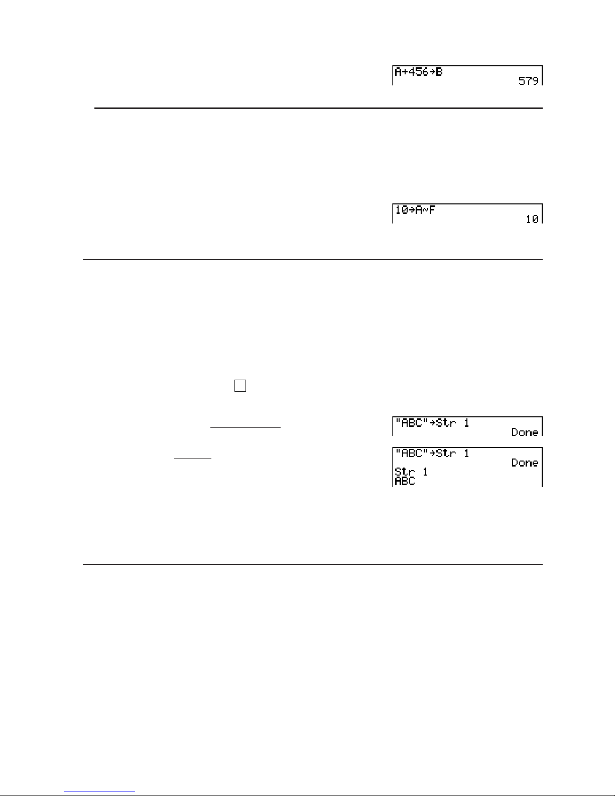
2-7

Example 2 To add 456 to variable A and store the result in variable B

?T(A)CDE?

?J(B)U

S To assign the same value to more than one variable

[value]? [first variable name]?(~) [last variable name]U

• You cannot use “

r”or“

Q

” as a variable name.

Example To assign a value of 10 to variables A through F

@???T(A) ?(~)?R(F)U

S String Memory

You can store up to 20 strings (named Str 1 to Str 20) in string memory. Stored strings can be output to the display or used inside functions and commands that support the use of strings as arguments.

For details about string operations, see “Strings” (page 8-18).

Example To assign string “ABC” to Str 1 and then output Str 1 to the display

?(

-LOCK)$(”)T(A) J(B)((C)$(”)?(Releases Alpha Lock.) ?)(E)(Str)*@U

(Str)*@U * fx-7400GII: (Str)

String is displayed justified left.

• Perform the above operation in the Linear input/output mode. It cannot be performed in the

Math input/output mode.

S Function Memory [OPTN]-[FMEM]

Function memory is convenient for temporary storage of often-used expressions. For longer term storage, we recommend that you use the GRAPH mode for expressions and the PRGM mode for programs.

• {STO}/{RCL}/{fn}/{SEE} ... {function store}/{function recall}/{function area specification as a

variable name inside an expression}/{function list}

2-8

S To store a function

Example To store the function (A+B) (A–B) as function memory number 1

?T(A)?J(B) ?T(A)?J(B)

*(E)(E)(FMEM)* (STO)@U * fx-7400G

II: (FMEM)

)))

• If the function memory number to which you store a function already contains a function, the

previous function is replaced with the new one.

• You can also use ? to store a function in function

memory in a program. In this case, you must enclose the function inside of double quotation marks.

S To recall a function

Example To recall the contents of function memory number 1

*(E)(E)(FMEM)* (RCL)@U * fx-7400G

II: (FMEM)

• The recalled function appears at the current location of the cursor on the display.

S To recall a function as a variable

B??T(A)U @??J(B)U *(E)(E)(FMEM)*(fn) @AU * fx-7400G

II: (FMEM)

S To display a list of available functions

*(E)(E)(FMEM)* (SEE) * fx-7400G

II: (FMEM)

2-9

S To delete a function

Example To delete the contents of function memory number 1

*(E)(E)(FMEM)* (STO)@U * fx-7400G

II: (FMEM)

• Executing the store operation while the display is blank deletes the function in the function

memory you specify.

I Answer Function

The Answer Function automatically stores the last result you calculated by pressing U (unless the U key operation results in an error).The result is stored in the answer memory.

• The largest value that the answer memory can hold is 15 digits for the mantissa and 2 digits

for the exponent.

• Answer memory contents are not cleared when you press the key or when you switch

power off.

S To use the contents of the answer memory in a calculation

Example 123 + 456 = 579

789 – 579 = 210

@ABCDEU FGH(Ans)U

fx-7400G

II, fx-9750GII users...

• The answer memory contents are not changed by an operation that assigns values to Alpha

memory (such as: D??J(B)U).

fx-9860G

II SD, fx-9860GII, fx-9860G AU PLUS, fx-9860G Slim users...

• In the Math input/output mode, the operation to recall answer memory contents is different

from the operation in the Linear input/output mode. For details, see “History Function” (page 1-17).

• Performing an operation that assigns a value to an Alpha memory (such as

D??J(B)U), answer memory contents are updated in the Math input/output mode but not in the Linear input/output mode.

2-10

I Performing Continuous Calculations

Answer memory also lets you use the result of one calculation as one of the arguments in the next calculation.

Example 1 w 3 =

1 w 3 s 3 =

@BU (Continuing)BU

Continuous calculations can also be used with Type B functions (

, x–1, x!, on page 2-2), +, –,

^(xy),x, ° ’ ”, etc.

3. Specifying the Angle Unit and Display Format

Before performing a calculation for the first time, you should use the Setup screen to specify the angle unit and display format.

I Setting the Angle Unit [SET UP]- [Angle]

1. On the Setup screen, highlight “Angle”.

2. Press the function key for the angle unit you want to specify, then press ).

• {Deg}/{Rad}/{Gra} ... {degrees}/{radians}/{grads}

• The relationship between degrees, grads, and radians is shown below. 360° = 2P radians = 400 grads 90° = P/2 radians = 100 grads

I Setting the Display Format [SET UP]- [Display]

1. On the Setup screen, highlight “Display”.

2. Press the function key for the item you want to set, then press ).

• {Fix}/{Sci}/{Norm}/{Eng} ... {fixed number of decimal places specification}/

{number of significant digits specification}/{normal display}/{Engineering mode}

S To specify the number of decimal places (Fix)

Example To specify two decimal places

(Fix)AU

Press the number key that corresponds to the number of decimal places you want to specify (

n = 0 to 9).

• Displayed values are rounded off to the number of decimal places you specify.

2-11

S To specify the number of significant digits (Sci)

Example To specify three significant digits

(Sci)BU

Press the number key that corresponds to the number of significant digits you want to specify (

n = 0 to 9). Specifying 0 makes the number of significant digits 10.

• Displayed values are rounded off to the number of significant digits you specify.

S To specify the normal display (Norm 1/Norm 2)

Press (Norm) to switch between Norm 1 and Norm 2.

Norm 1: 10

–2

(0.01) > |x|, |x| 10

Norm 2: 10–9(0.000000001) > |x|, |x| 10

S To specify the engineering notation display (Eng mode)

Press (Eng) to switch between engineering notation and standard notation.The indicator “/E” is on the display while engineering notation is in effect.

You can use the following symbols to convert values to engineering notation, such as 2,000 (= 2 × 10

) m 2k.

E (Exa)

s 10

m (milli)

s 10

–3

P (Peta)

s 10

M (micro) s 10

–6

T(Tera)

s 10

n (nano)

s 10

–9

G (Giga)

s 10

p (pico)

s 10

–12

M (Mega)

s 10

f (femto)

s 10

–15

k (kilo)

s 10

• The engineering symbol that makes the mantissa a value from 1 to 1000 is automatically

selected by the calculator when engineering notation is in effect.

4. Function Calculations

I Function Menus

This calculator includes five function menus that give you access to scientific functions not printed on the key panel.

• The contents of the function menu differ according to the mode you entered from the Main

Menu before you pressed the * key. The following examples show function menus that appear in the RUN • MAT (or RUN)orPRGM mode.

2-12

S Hyperbolic Calculations (HYP) [OPTN]-[HYP]

• {sinh}/{cosh}/{tanh} ... hyperbolic {sine}/{cosine}/{tangent}

• {sinh

–1

}/{cosh–1}/{tanh–1} ... inverse hyperbolic {sine}/{cosine}/{tangent}

S Probability/Distribution Calculations (PROB) [OPTN]-[PROB]

• {

x!} ... {press after inputting a value to obtain the factorial of the value}

• {

nPr}/{nCr} ... {permutation}/{combination}

• {RAND} ... {random number generation}

• {Ran#}/{Int}/{Norm}/{Bin}/{List} ... {random number generation (0 to 1)}/{random integer generation}/{random number generation in accordance with normal distribution based on mean

ƫ and standard deviation Ʊ}/{random number generation in accordance with

binomial distribution based on number of trials n and probability p}/{random number generation (0 to 1) and storage of result in ListAns}

• {P(}/{Q(}/{R(} ... normal probability {P(

t)}/{Q(t)}/{R(t)}

• {

t(} ... {value of normalized variate t(x)}

S Numeric Calculations (NUM) [OPTN]-[NUM]

• {Abs} ... {select this item and input a value to obtain the absolute value of the value}

• {Int}/{Frac} ... select the item and input a value to extract the {integer}/{fraction} part.

• {Rnd} ... {rounds off the value used for internal calculations to 10 significant digits (to match the value in the answer memory), or to the number of decimal places (Fix) and number of significant digits (Sci) specified by you}

• {Intg} ... {select this item and input a value to obtain the largest integer that is not greater than the value}

• {RndFi} ... {rounds off the value used for internal calculations to specified digits (0 to 9) (see

page 2-2).}

• {GCD} ... {greatest common divisor for two values}

• {LCM} ... {least common multiple for two values}

• {MOD} ... {remainder of division (remainder output when

n is divided by m)}

• {MOD

•

E} ... {remainder when division is performed on a power value (remainder output

when n is raised to p power and then divided by m)}

S Angle Units, Coordinate Conversion, Sexagesimal Operations (ANGL)

[OPTN]-[ANGL]

• {°}/{r}/{g} ... {degrees}/{radians}/{grads} for a specific input value

• {°’”} ... {specifies degrees (hours), minutes, seconds when inputting a degrees/minutes/ seconds value}

•{

°’”

} ... {converts decimal value to degrees/minutes/seconds value}

• The {

°’”

} menu operation is available only when there is a calculation result on the display.

• {Pol(}/{Rec(} ... {rectangular-to-polar}/{polar-to-rectangular} coordinate conversion

• {DMS} ... {converts decimal value to sexagesimal value}

2-13

S Engineering Symbol (ESYM) [OPTN]-[ESYM]

• {m}/{

μ}/{n}/{p}/{f} ... {milli (10

–3

)}/{micro (10–6)}/{nano (10–9)}/{pico (10

–12

)}/{femto (10

–15

)}

• {k}/{M}/{G}/{T}/{P}/{E} ... {kilo (10

)}/{mega (106)}/{giga (109)}/{tera (1012)}/{peta (1015)}/

{exa (1018)}

• {ENG}/{ENG} ... shifts the decimal place of the displayed value three digits to the {left}/{right} and {decreases}/{increases} the exponent by three.

When you are using engineering notation, the engineering symbol is also changed

accordingly.

• The {ENG} and {ENG} menu operations are available only when there is a calculation result

on the display.

I Angle Units

• Be sure to specify Comp for Mode in the Setup screen.

Example Operation

To convert 4.25 rad to degrees:

243.5070629

K(SET UP)AAAAAA*(Deg))

4.25*(E)(ANGL)**(r)U

47.3° + 82.5rad = 4774.20181°

47.382.5*(E)(ANGL)**(r)U

2°20´30˝ + 39´30˝ = 3°00´00˝

2*(E)(ANGL)**(° ’ ”) 20(° ’ ”) 30 (° ’ ”)0(° ’ ”)39(° ’ ”) 30(° ’ ”)U (

°’”

)

2.255° = 2°15´18˝

2.255*(E)(ANGL)**(E)(DMS)U

* fx-7400G

II, fx-9750GII: AAAAA ** fx-7400GII: (ANGL)

I Trigonometric and Inverse Trigonometric Functions

• Be sure to set the angle unit before performing trigonometric function and inverse trigonometric function calculations.

• Be sure to specify Comp for Mode in the Setup screen.

Example Operation

cos (



rad) = 0.5

K(SET UP)AAAAAA*(Rad)) A$(P)3U

•

sin 45° s cos 65° = 0.5976724775

K(SET UP)AAAAAA*(Deg)) 2Q45A65U*

sin–10.5 = 30° (

x when sinx = 0.5)

Q(sin

–1

) 0.5*2U

 can be omitted. * fx-7400GII, fx-9750GII: AAAAA

Input of leading zero is not necessary.

(90° = radians = 100 grads)



(90° = radians = 100 grads)



2-14

I Logarithmic and Exponential Functions

• Be sure to specify Comp for Mode in the Setup screen.

Example Operation

log 1.23 (log

1.23) = 0.08990511144

J1.23U

log

8=3

*(CALC)*(E)(logab)28U

(–3)

= (–3) s (–3) s (–3) s (–3) = 81

3,4U

123 (= 123

1 7

) = 1.988647795

7,(

)123U

* fx-7400G

II: (CALC)

• The Linear input/output mode and Math input/output mode produce different results when two or more powers are input in series, like: 2 , 3 , 2.

Linear input/output mode: 2^3^2 = 64 Math input/output mode:

= 512

This is because the Math input/output mode internally treats the above input as: 2^(3^(2)).

I Hyperbolic and Inverse Hyperbolic Functions

• Be sure to specify Comp for Mode in the Setup screen.

Example Operation

sinh 3.6 = 18.28545536

*(E)(HYP)*(sinh)3.6U

cosh

–1

= 0.7953654612

*(E)(HYP)*(cosh–1)2015U

* fx-7400G

II: (HYP)

I Other Functions

• Be sure to specify Comp for Mode in the Setup screen.

Example Operation

2+5 = 3.65028154

V()2V()5U

(–3)

= (–3) s (–3) = 9

3VU

8! (= 1 s 2 s 3 s .... s 8) = 40320

8*(E)(PROB)*1(x!)U

What is the integer part of – 3.5?

–3

*(E)(NUM)*2(Int)3.5U

*1fx-7400GII: (PROB) *2fx-7400GII: (NUM)

2-15

I Random Number Generation (RAND)

S Random Number Generation (0 to 1) (Ran#, RanList#)

Ran# and RanList# generate 10 digit random numbers randomly or sequentially from 0 to 1. Ran# returns a single random number, while RanList# returns multiple random numbers in list form. The following shows the syntaxes of Ran# and RanList#.

Ran# [a] 1 

a  9

RanList# (n [,a]) 1 

n  999

•

n is the number of trials. RanList# generates the number of random numbers that

corresponds to n and displays them on the ListAns screen. A value must be input for n.

• “

a” is the randomization sequence. Random numbers are returned if nothing is input for “a”.

Entering an integer of 1 through 9 for

a will return the corresponding sequential random

number.

• Executing the function Ran# 0 initializes the sequences of both Ran# and RanList#. The sequence also is initialized when a sequential random number is generated with a different sequence of the previous execution using Ran# or RanList#, or when generating a random number.

Ran# Examples

Example Operation

Ran# (Generates a random number.)

*(E)(PROB)*(RAND) (Ran#)U

(Each press of U generates a new random number.)

U U

Ran# 1 (Generates the first random number in sequence 1.)

(Generates the second random number in sequence 1.)

*(E)(PROB)*(RAND) (Ran#)1U

Ran# 0 (Initializes the sequence.)

Ran# 1 (Generates the first random number in sequence 1.)

(Ran#)0U

(Ran#)1U

* fx-7400G

II: (PROB)

2-16

RanList# Examples

Example Operation

RanList# (4) (Generates four random numbers and displays the result on the ListAns screen.)

*(E)(PROB)*(RAND)(List)

4U

RanList# (3, 1) (Generates from the first to the third random numbers of sequence 1 and displays the result on the ListAns screen.)

)*(E)(PROB)*(RAND) (List) 31U

(Next, generates from the fourth to the sixth random number of sequence 1 and displays the result on the ListAns screen.)

Ran# 0 (Initializes the sequence.)

)(Ran#)0U

RanList# (3, 1) (Re-generates from the first to the third random numbers of sequence 1 and displays the result on the ListAns screen.)

(List)31U

* fx-7400G

II: (PROB)

S Random Integer Generation (RanInt#)

RanInt# generates random integers that fall between two specified integers. RanInt# (A, B [,n]) A < B |A|,|B| < 1

E10 B–A<1E10 1  n  999

• A is the start value and B is the end value. Omitting a value for

n returns a generated random

number as-is. Specifying a value for n returns the specified number of random values in list form.

Example Operation

RanInt# (1, 5) (Generates one random integer from 1 and

5.)

*(E)(PROB)*(RAND)(Int)

15U

RanInt# (1, 10, 5) (Generates five random integers from 1 to 10 and displays the result on the ListAns screen.)

*(E)(PROB)*(RAND)(Int)

1105U

* fx-7400GII: (PROB)

S Random Number Generation in Accordance with Normal Distribution

(RanNorm#)

This function generates a 10-digit random number in accordance with normal distribution based on a specified mean ƫ and standard deviation Ʊ values.

RanNorm# (

Ʊ, ƫ [,n]) Ʊ >0 1 n  999

• Omitting a value for

n returns a generated random number as-is. Specifying a value for n

returns the specified number of random values in list form.

2-17

Example Operation

RanNorm# (8, 68) (Randomly produces a body length value obtained in accordance with the normal distribution of a group of infants less than one year old with a mean body length of 68cm and standard deviation of 8.)

*(E)(PROB)*(RAND)(Norm)

868U

RanNorm# (8, 68, 5) (Randomly produces the body lengths of five infants in the above example, and displays them in a list.)

*(E)(PROB)*(RAND)(Norm)

8685U

* fx-7400G

II: (PROB)

S Random Number Generation in Accordance with Binomial Distribution

(RanBin#)

This function generates random integers in accordance with binomial distribution based on values specified for the number of trials n and probability p.

RanBin# (n, p [,m]) 1 

n  100000 1  m  999 0  p  1

• Omitting a value for

m returns a generated random number as-is. Specifying a value for m

returns the specified number of random values in list form.

Example Operation

RanBin# (5, 0.5) (Randomly produces the number of heads that can be expected in accordance with binomial distribution for five coin tosses where the probability of heads is 0.5.)

*(E)(PROB)*(RAND)(Bin)

50.5U

RanBin# (5, 0.5, 3) (Performs the same coin toss sequence described above three times and displays the results in a list.)

*(E)(PROB)*(RAND)(Bin)

50.53U

* fx-7400GII: (PROB)

I Coordinate Conversion

S Rectangular Coordinates S Polar Coordinates

• With polar coordinates,

Ƨ can be calculated and displayed within a range of

–180°< Ƨ  180° (radians and grads have same range).

• Be sure to specify Comp for Mode in the Setup screen.

2-18

Example Operation

Calculate

r and Ƨ° when x =14andy = 20.7

K(SET UP)AAAAAA* (Deg)) *(E)(ANGL)**(E)(Pol() 1420.7U)

Calculate

x and y when r =25andƧ = 56°

(Rec()2556U

* fx-7400G

II, fx-9750GII: AAAAA ** fx-7400GII: (ANGL)

I Permutation and Combination

S Permutation S Combination

• Be sure to specify Comp for Mode in the Setup screen.

Example 1 To calculate the possible number of different arrangements using 4

items selected from among 10 items

Formula Operation

10P4 = 5040

10*(E)(PROB)*(nPr)4U

* fx-7400G

II: (PROB)

Example 2 To calculate the possible number of different combinations of 4 items

that can be selected from among 10 items

Formula Operation

10C4 = 210

10*(E)(PROB)*(nCr)4U

* fx-7400G

II: (PROB)

I Greatest Common Divisor (GCD), Least Common Multiple (LCM)

Example Operation

To determine the greatest common divisor of 28 and 35 (GCD (28, 35) = 7)

*(E)(NUM)*(E)(GCD)28 35U

To determine the least common multiple of 9 and 15 (LCM (9, 15) = 45)

*(E)(NUM)*(E)(LCM)915 U

* fx-7400G

II: (NUM)

1 24.98924.98979792 (r) 2 55.928  55.92839019 ( )



1 24.98924.98979792 (r) 2 55.928  55.92839019 ( )



1 13.97913.97982259 (x) 2 20.725  20.72593931 (y)

nPr

nCr

(

n–r

r!(n–r

nPr

nCr

(

n–r

r!(n–r

2-19

I Division Remainder (MOD), Remainder of Exponential Division (MOD

Exp)

Example Operation

To determine the remainder when 137 is divided by 7 (MOD (137, 7) = 4)

*(E)(NUM)*(E)(MOD)1377 U

To determine the remainder when 53is divided by 3 (MOD•E (5, 3, 3) = 2)

*(E)(NUM)*(E)(MOD•E)

533U

* fx-7400GII: (NUM)

I Fractions

• In the Math input/output mode, the fraction input method is different from that described below. For fraction input operations in the Math input/output mode, see page 1-11.

• Be sure to specify Comp for Mode in the Setup screen.

Example Operation

2173

–

–+3––=––

–

5420

= 3.65 (Conversion to decimal)*

25314U

–

–––– + ––––

–

2578 4572

= 6.066202547 s 10

–4*2

1257814572U

–

s 0.5 = 0.25*

12.5U

Fractions can be converted to decimal values and vice versa.

When the total number of characters, including integer, numerator, denominator and delimiter

marks exceeds 10, the fraction is automatically displayed in decimal format.

Calculations containing both fractions and decimals are calculated in decimal format.

• Pressing the ,(



) key toggles the display fraction between mixed fraction and

improper fraction format.

I Engineering Notation Calculations

Input engineering symbols using the engineering notation menu.

• Be sure to specify Comp for Mode in the Setup screen.

Example Operation

999k (kilo) + 25k (kilo)

= 1.024M (mega)

K(SET UP)DD(Eng))999*(E)(E) (ESYM)*(E)(k)25(k)U

9 w 10 = 0.9 = 900m (milli) = 0.9

910U

*(E)(E)(ESYM)*(E)(E)(ENG)*

2-20

= 0.0009k (kilo) = 0.9 = 900m

(ENG)*

(ENG)*

* fx-7400GII: (ESYM)

Converts the displayed value to the next higher engineering unit, by shifting the decimal point three places to the right.

Converts the displayed value to the next lower engineering unit, by shifting the decimal point three places to the left.

I Logical Operators (AND, OR, NOT, XOR) [OPTN]-[LOGIC]

The logical operator menu provides a selection of logical operators.

• {And}/{Or}/{Not}/{Xor} ... {logical AND}/{logical OR}/{logical NOT}/{logical XOR}

• Be sure to specify Comp for Mode in the Setup screen.

Example What is the logical AND of A and B whenA=3andB=2?

AANDB=1

Operation Display

3??T(A)U

2??J(B)U

?T(A)*(E)(E)

(LOGIC)*(And)?J(B)U

* fx-7400G

II: (LOGIC)

S About Logical Operations

• A logical operation always produces either 0 or 1 as its result.

• The following table shows all of possible results that can be produced by AND, OR and XOR operations.

Value or Expression A Value or Expression B A AND B A OR B A XOR B

A x 0Bx 0

110

A x 0

B=0 0 1 1

A=0

B x 0

011

A=0 B=0 0 0 0

• The following table shows the results produced by the NOT operation.

Value or Expression A NOT A

A x 0

A=0 1

2-21

5. Numerical Calculations

The following explains the numerical calculation operations included in the function menu displayed when *(CALC) ((CALC) on the fx-7400G

II) is pressed. The following

calculations can be performed.

• {Int÷}/{Rmdr}/{Simp} ... {quotient}/{remainder}/{simplification}

• {Solve}/{

d/dx}/{d

/dx2}/{°dx}/{SolvN} ... {equality solution}/{differential}/{quadratic differential}/

{integration}/{f(x) function solution}

• {FMin}/{FMax}/{3(}/{log

b} ... {minimum value}/{maximum value}/{summation}/{logarithm

logab}

I Quotient of Integer ÷ Integer [OPTN]-[CALC]-[Int÷]

The “Int÷” function can be used to determine the quotient when one integer is divided by another integer.

Example To calculate the quotient of 107 ÷ 7

@?F*(CALC)*(E) (E)(Int÷)F U * fx-7400G

II: (CALC)

I Remainder of Integer ÷ Integer [OPTN]-[CALC]-[Rmdr]

The “Rmdr” function can be used to determine the remainder when one integer is divided by another integer.

Example To calculate the remainder of 107 ÷ 7

@?F*(CALC)*(E) (E)(Rmdr)F U * fx-7400G

II: (CALC)

I Simplification [OPTN]-[CALC]-[Simp]

The “Simp” function can be used to simplify fractions manually. The following operations can be used to perform simplification when an unsimplified calculation result is on the display.

• {Simp} U ... This function automatically simplifies the displayed calculation result using the

smallest prime number available. The prime number used and the simplified result are shown on the display.

• {Simp}

n U ... This function performs simplification according to the specified divisor n.

2-22

Under initial default settings, this calculator automatically simplifies fraction calculation results before displaying them. Before performing the following examples, use the Setup screen to change the “Simplify” setting from “Auto” to “Manual” (page 1-29).

• When “a+b

i”or“r

” is specified for the Setup screen “Complex Mode” setting, fraction calculation results always are simplified before being displayed, even if the “Simplify” setting is “Manual”.

• If you want to simplify fractions manually (Simplify: Manual), make sure that the “Real” is selected for the “Complex Mode” setting.

Example 1 To simplify

15 60

2014

@DE?U *(CALC)*(E)(E)(Simp)U

* fx-7400GII: (CALC)

(Simp)U

The “F=” value is the divisor.

Example 2 To simplify

27 63

specifying a divisor of 9

27 63

3 7

AFEBU*(CALC)* (E)(E)(Simp)HU

* fx-7400G

II: (CALC)

• An error occurs if simplification cannot be performed using the specified divisor.

• Executing Simp while a value that cannot be simplified is displayed will return the original value, without displaying “F=”.

I Solve Calculations [OPTN]-[CALC]-[Solve]

The following is the syntax for using the Solve function in a program.

Solve(

f(x), n, a, b)(a: lower limit, b: upper limit, n: initial estimated value)

There are two different input methods that can be used for Solve calculations: direct assignment and variable table input.

With the direct assignment method (the one described here), you assign values directly to variables.This type of input is identical to that used with the Solve command used in the PRGM mode.

2-23

Variable table input is used with the Solve function in the EQUA mode.This input method is recommended for most normal Solve function input.

An error (Time Out) occurs when there is no convergence of the solution. For information about Solve calculations, see page 4-4.

• You cannot use a quadratic differential, 3, maximum/minimum value or Solve calculation expression inside of any of the above functions.

• Pressing during calculation of Solve (while the cursor is not shown on the display) interrupts the calculation.

I Solving an f(x) Function [OPTN]-[CALC]-[SolvN]

You can use SolvN to solve an

f(x) function using numerical analysis. The following is the input

syntax.

SolveN (left side [=right side] [,variable] [, lower limit, upper limit])

• The right side, variable, lower limit and upper limit all can be omitted.

• “left side[=right side]” is the expression to be solved. Supported variables are A through Z,

and

. When the right side is omitted, solution is perform using right side = 0.

• The variable specifies the variable within the expression to be solved for (A through Z,

Omitting a variable specification cause X to be used as the variable.

• The lower limit and upper limit specify the range of the solution. You can input a value or an expression as the range.

• The following functions cannot be used within any of the arguments.

Solve(,

/dx2, FMin(, FMax(, 3(

Up to 10 calculation results can be displayed simultaneously in ListAns format.

• The message “No Solution” is displayed if no solution exists.

• The message “More solutions may exist.” is displayed when there may be solutions other than those displayed by SolvN.

Example To solve

–5x –6=0

*(CALC)*(SolvN) TVDTEU

* fx-7400GII: (CALC)

)

2-24

I Differential Calculations [OPTN]-[CALC]-[d/dx]

To perform differential calculations, first display the function analysis menu, and then input the values using the syntax below.

*(CALC)* (

d/dx) f(x)atol * fx-7400GII: (CALC)

(

a: point for which you want to determine the derivative, tol: tolerance)

The differentiation for this type of calculation is defined as:

In this definition, infinitesimal is replaced by a sufficiently small

x, with the value in the

neighborhood of f'(a) calculated as:

In order to provide the best precision possible, this unit employs central difference to perform differential calculations.

Example To determine the derivative at point

x = 3 for the function

y = x

+4x2+ x – 6, with a tolerance of “tol”=1E –5

Input the function f(x).

*(CALC)* (

d/dx)T,BCTVTE

* fx-7400G

II: (CALC)

Input point

x = a for which you want to determine the derivative.

B

Input the tolerance value.

@$DU

Using Differential Calculation in a Graph Function

• Omitting the tolerance (tol) value when using the differential command inside of a graph function simplifies the calculation for drawing the graph. In such a case, precision is sacrificed for the sake of faster drawing.The tolerance value is specified, the graph is drawn with the same precision obtained when you normally perform a differential calculation.

• You can also omit input of the derivative point by using the following format for the differential graph:Y2=

d/dx(Y1). In this case, the value of the X variable is used as the derivative point.

Differential Calculation Precautions

• In the function f(x), only X can be used as a variable in expressions. Other variables (A through Z excluding X, r, Ƨ) are treated as constants, and the value currently assigned to that variable is applied during the calculation.

• Input of the tolerance (

tol) value and the closing parenthesis can be omitted. If you omit

tolerance (tol) value, the calculator automatically uses a value for tol as 1E–10.

• Specify a tolerance (

tol) value of 1E–14 or greater. An error (Time Out) occurs whenever no

solution that satisfies the tolerance value can be obtained.

• Pressing during calculation of a differential (while the cursor is not shown on the display) interrupts the calculation.

d/dx

(f

(x)

,

)



(a)

d/dx

(f

(x)

,

)



(a)

f(a

x)–f(a

)

f(a

) = lim

–––––––––––––





f(a

x)–f(a

)

f(a

) = lim

–––––––––––––





f(a

x)–f(a

)

f(a

)

–––––––––––––



f(a

x)–f(a

)

f(a

)

–––––––––––––



2-25

• Inaccurate results and errors can be caused by the following:

- discontinuous points in

x values

- extreme changes in

x values

- inclusion of the local maximum point and local minimum point in

x values

- inclusion of the inflection point in

x values

- inclusion of undifferentiable points in

x values

- differential calculation results approaching zero

• Always use radians (Rad mode) as the angle unit when performing trigonometric differentials.

• You cannot use a differential, quadratic differential, integration, 3, maximum/minimum value, Solve, RndFix or log

b calculation expression inside a differential calculation term.

• In the Math input/output mode, the tolerance value is fixed at 1

E–10 and cannot be changed.

I Quadratic Differential Calculations [OPTN]-[CALC]-[d2/dx

]

After displaying the function analysis menu, you can input quadratic differentials using the following syntax.

*(CALC)*(

/dx2) f(x)atol * fx-7400GII: (CALC)

(

a: differential coefficient point, tol: tolerance)

Quadratic differential calculations produce an approximate differential value using the following second order differential formula, which is based on Newton’s polynomial interpretation.

In this expression, values for “sufficiently small increments of

h” are used to obtain a value that

approximates f"(a).

Example To determine the quadratic differential coefficient at the point where

x = 3 for the function y = x

+4x2+ x –6

Here we will use a tolerance tol =1E –5

Input the function

f(x).

*(CALC)* (

/dx2) T,BCTVTE

* fx-7400G

II: (CALC)

Input 3 as point

a, which is the differential coefficient point.

B

Input the tolerance value.

@$D

Quadratic Differential Calculation Precautions

–

–– (

f(x),a

)



–––

f(a

)

–

–– (

f(x),a

)



–––

f(a

)

''(a) =

180h

2 f(a + 3h) – 27 f(a + 2h) + 270 f(a + h) – 490 f(a) + 270 f(a – h) – 27 f(a –2h) + 2 f(a – 3h)

''(a) =

180h

2 f(a + 3h) – 27 f(a + 2h) + 270 f(a + h) – 490 f(a) + 270 f(a – h) – 27 f(a –2h) + 2 f(a – 3h)

2-26

• Input of the tolerance (tol) value and the closing parenthesis can be omitted.

• Specify a tolerance (

tol) value of 1E–14 or greater. An error (Time Out) occurs whenever no

solution that satisfies the tolerance value can be obtained.

• The rules that apply for linear differential also apply when using a quadratic differential calculation for the graph formula (see page 2-24).

• Inaccurate results and errors can be caused by the following:

- discontinuous points in

x values

- extreme changes in

x values

- inclusion of the local maximum point and local minimum point in

x values

- inclusion of the inflection point in

x values

- inclusion of undifferentiable points in

x values

- differential calculation results approaching zero

• You can interrupt an ongoing quadratic differential calculation by pressing the key.

• Always use radians (Rad mode) as the angle unit when performing trigonometric quadratic differentials.

• You cannot use a differential, quadratic differential, integration, 3, maximum/minimum value, Solve, RndFix or log

b calculation expression inside of a quadratic differential calculation

term.

• With quadratic differential calculation, calculation precision is up to five digits for the mantissa.

• In the Math input/output mode, the tolerance value is fixed at 1

E–10 and cannot be changed.

I Integration Calculations [OPTN]-[CALC]-[°dx]

To perform integration calculations, first display the function analysis menu and then input the values using the syntax below.

*(CALC)* (°

dx) f(x)  a  b  tol  * fx-7400GII: (CALC)

(

: start point,b: end point,

tol

: tolerance)

Area of





f(x)dx

is calculated

As shown in the illustration above, integration calculations are performed by calculating integral values from

a through b for the function y = f (x) where a  x  b, and f (x)  0. This in

effect calculates the surface area of the shaded area in the illustration.





f(x),a

b, tol

)







f(x)d





f(x),a

b, tol

)







f(x)d

2-27

Example To perform the integration calculation for the function shown below,

with a tolerance of “

tol”=1E –4

Input the function f (x).

*(CALC)* (°

dx)ATVBTC

* fx-7400G

II: (CALC)

Input the start point and end point.

@D

Input the tolerance value.

@$CU

Note the following points to ensure correct integration values.

(1) When cyclical functions for integration values become positive or negative for different

divisions, perform the calculation for single cycles, or divide between negative and positive, and then add the results together.

Positive part (

)

Negative part (

)

Positive part (S) Negative part (S)

(2) When minute fluctuations in integration divisions produce large fluctuations in integration

values, calculate the integration divisions separately (divide the large fluctuation areas into smaller divisions), and then add the results together.

• Pressing during calculation of an integral (while the cursor is not shown on the display) interrupts the calculation.

• Always use radians (Rad mode) as the angle unit when performing trigonometric integrations.

• An error (Time Out) occurs whenever no solution that satisfies the tolerance value can be obtained.



(2x2 + 3x + 4) dx



(2x2 + 3x + 4) dx





f(x)dx =





f(x)dx

+ (–





f(x)dx

)





f(x)dx =





f(x)dx

+ (–





f(x)dx

)





f(x)dx =





f(x)dx





f(x)dx

+.....+





f(x)dx





f(x)dx =





f(x)dx





f(x)dx

+.....+





f(x)dx

2-28

Integration Calculation Precautions

• In the function f(x), only X can be used as a variable in expressions. Other variables (A through Z excluding X,

r, Ƨ) are treated as constants, and the value currently assigned to

that variable is applied during the calculation.

• Input of “

tol” and closing parenthesis can be omitted. If you omit “tol,” the calculator

automatically uses a default value of 1E–5.

• Integration calculations can take a long time to complete.

• You cannot use a differential, quadratic differential, integration, 3, maximum/minimum value, Solve, RndFix or log

b calculation expression inside of an integration calculation term.

• In the Math input/output mode, the tolerance value is fixed at 1

E–5 and cannot be changed.

I 3 Calculations [OPTN]-[CALC]-[3(]

To perform 3 calculations, first display the function analysis menu, and then input the values using the syntax below.

*(CALC)* (E)(3()

ak  k 

B n  * fx-7400GII: (CALC)

(

n: distance between partitions)

Example To calculate the following:

Use

n = 1 as the distance between partitions.

*(CALC)*(E)(3()?(K) VB?(K)D ?(K)AE@U

* fx-7400G

II: (CALC)

3 Calculation Precautions

• The value of the specified variable changes during a 3 calculation. Be sure to keep separate written records of the specified variable values you might need later before you perform the calculation.

• You can use only one variable in the function for input sequence

ak.

• Input integers only for the initial term (

) of sequence ak and last term (B) of sequence ak.

• Input of

n and the closing parentheses can be omitted. If you omit n, the calculator

automatically uses n =1.

• Make sure that the value used as the final term

is greater than the value used as the initial

term

. Otherwise, an error will occur.

• To interrupt an ongoing 3 calculation (indicated when the cursor is not on the display), press the key.

• You cannot use a differential, quadratic differential, integration, 3, maximum/minimum value, Solve, RndFix or log

b calculation expression inside of a 3 calculation term.

• In the Math input/output mode, the distance between partitions (

n) is fixed at 1 and cannot be

changed.





(

,

)





+........+



k =







(

,

)





+........+



k =





(

–3k+5)

k = 2



(

–3k+5)

k = 2

2-29

I Maximum/Minimum Value Calculations [OPTN]-[CALC]-[FMin]/[FMax]

After displaying the function analysis menu, you can input maximum/minimum calculations using the formats below, and solve for the maximum and minimum of a function within interval

a  x  b.

S Minimum Value

*(CALC)* (E)(FMin) f (x)  a  b  n  * fx-7400GII: (CALC) (

a: start point of interval, b: end point of interval, n: precision (n =1to9))

S Maximum Value

*(CALC)* (E)(FMax) f (x) a  b  n  * fx-7400GII: (CALC) (

a: start point of interval, b: end point of interval, n: precision (n =1to9))

Example To determine the minimum value for the interval defined by start

point

a = 0 and end point b = 3, with a precision of n = 6 for the function

y = x

–4x +9

Input f (x).

*(CALC)* (E)(FMin)TVCTH * fx-7400G

II: (CALC)

Input the interval

a =0,b =3.

?B

Input the precision

n =6.

EU

• In the function

f (x), only X can be used as a variable in expressions. Other variables (A

through Z excluding X, r, Ƨ) are treated as constants, and the value currently assigned to that variable is applied during the calculation.

• Input of

n and the closing parenthesis can be omitted.

• Discontinuous points or sections with drastic fluctuation can adversely affect precision or even cause an error.

• Inputting a larger value for

n increases the precision of the calculation, but it also increases

the amount of time required to perform the calculation.

• The value you input for the end point of the interval (

b) must be greater than the value you

input for the start point (

a). Otherwise an error occurs.

• You can interrupt an ongoing maximum/minimum calculation by pressing the key.

• You can input an integer in the range of 1 to 9 for the value of

n. Using any value outside this

range causes an error.

• You cannot use a differential, quadratic differential, integration, 3, maximum/minimum value, Solve, RndFix or log

b calculation expression inside of a maximum/minimum calculation

term.

2-30

6. Complex Number Calculations

You can perform addition, subtraction, multiplication, division, parentheses calculations, function calculations, and memory calculations with complex numbers just as you do with the manual calculations described on pages 2-1 to 2-14.

You can select the complex number calculation mode by changing the Complex Mode item on the Setup screen to one of the following settings.

•{Real} ... Calculation in the real number range only*

•{a+bi} ... Performs complex number calculation and displays results in rectangular form

•{

rƧ} ... Performs complex number calculation and displays results in polar form*

*1 When there is an imaginary number in the argument, however, complex number calculation

is performed and the result is displayed using rectangular form. Examples: ln 2

i = 0.6931471806 + 1.570796327i

ln 2i + ln (– 2) = (Non-Real ERROR)

The display range of Ƨ depends on the angle unit set for the Angle item on the Setup

screen.

• Deg ... –180 <

Ƨ  180

• Rad ... – P <

Ƨ  P

• Gra ... –200 <

Ƨ  200

Press *(CPLX) (*(CPLX) on the fx-7400G

II) to display the complex calculation

number menu, which contains the following items.

•{

i} ... {imaginary unit i input}

•{Abs}/{Arg} ... obtains {absolute value}/{argument}

•{Conj} ... {obtains conjugate}

•{ReP}/{ImP} ... {real}/{imaginary} part extraction

•{rƧ}/{a+bi} ... converts the result to {polar}/{rectangular} form

• You can also use ?(

i) in place of *(CPLX) (*(CPLX) on the fx-7400GII)

(i).

• Solutions obtained by the Real,

a+bi and rƧ modes are different for power root (x

)

calculations when x < 0 and y = m/n when n is an odd number. Example: 3

 (– 8) = – 2 (Real)

= 1 + 1.732050808i (a+bi) = 260 (rƧ)

• To input the “  ” operator into the polar coordinate expression (

rƧ), press T().

2-31

I Arithmetic Operations [OPTN]-[CPLX]-[i]

Arithmetic operations are the same as those you use for manual calculations. You can even use parentheses and memory.

Example (1 + 2

i)+(2+3i)

*(CPLX)* @A(

i)

AB(

i)U

* fx-7400G

II: (CPLX)

I Reciprocals, Square Roots, and Squares

Example (3 + i)

*(CPLX)* V()B(

i)U

* fx-7400G

II: (CPLX)

I Complex Number Format Using Polar Form

Example 230 s 345=675

K(SET UP)AAAAAA* (Deg)A(

rƧ))

AT()B?B T()CDU

* fx-7400G

II, fx-9750GII: AAAAA

I Absolute Value and Argument [OPTN]-[CPLX]-[Abs]/[Arg]

The unit regards a complex number in the form

a + bi as a coordinate on a Gaussian plane,

and calculates absolute value²Z²and argument (arg).

Example To calculate absolute value (

r) and argument (Ƨ) for the complex number

3+4

i, with the angle unit set for degrees

Imaginary axis

Real axis

2-32

*(CPLX)*(Abs) BC(

i)U

(Calculation of absolute value) * fx-7400G

II: (CPLX)

*(CPLX)*(Arg) BC(

i)U

(Calculation of argument) * fx-7400G

II: (CPLX)

• The result of the argument calculation differs in accordance with the current angle unit setting (degrees, radians, grads).

I Conjugate Complex Numbers [OPTN]-[CPLX]-[Conj]

A complex number of the form

a + bi becomes a conjugate complex number of the form

a – bi.

Example To calculate the conjugate complex number for the complex number

2+4

*(CPLX)*(Conj) AC(

i)U

* fx-7400G

II: (CPLX)

I Extraction of Real and Imaginary Parts [OPTN]-[CPLX]-[ReP]/[lmP]

Use the following procedure to extract the real part

a and the imaginary part b from a complex

number of the form

a + bi.

Example To extract the real and imaginary parts of the complex number2+5

*(CPLX)*(E)(ReP) AD(E)(

i)U

(Real part extraction)

* fx-7400G

II: (CPLX)

*(CPLX)*(E)(ImP) AD(E)(

i)U

(Imaginary part extraction)

* fx-7400G

II: (CPLX)

I Polar and Rectangular Form Transformation [OPTN]-[CPLX]-[rƧ]/[a+bi]

Use the following procedure to transform a complex number displayed in rectangular form to polar form, and vice versa.

2-33

Example To transform the rectangular form of complex number 1 + 3 i to its

polar form

K(SET UP)AAAAAA* (Deg)A(

a+bi))

@V()B *(CPLX)**(

i)(E)(r

* fx-7400G

II, fx-9750GII: AAAAA

** fx-7400G

II: (CPLX)

AT()E?

*(CPLX)*(E)(

a+bi)U

* fx-7400G

II: (CPLX)

• The input/output range of complex numbers is normally 10 digits for the mantissa and two digits for the exponent.

• When a complex number has more than 21 digits, the real part and imaginary part are displayed on separate lines.

• The following functions can be used with complex numbers. ,

, x–1, ^(xy),3,x, In, log, logab, 10x, ex, Int, Frac, Rnd, Intg, RndFix(, Fix, Sci, ENG,

ENG, ° ’ ”,

° ’ ”

/c, d/c

7. Binary, Octal, Decimal, and Hexadecimal Calculations with Integers

You can use the RUN•MAT (or RUN) mode and binary, octal, decimal, and hexadecimal settings to perform calculations that involve binary, octal, decimal and hexadecimal values. You can also convert between number systems and perform bitwise operations.

• You cannot use scientific functions in binary, octal, decimal, and hexadecimal calculations.

• You can use only integers in binary, octal, decimal, and hexadecimal calculations, which

means that fractional values are not allowed. If you input a value that includes a decimal part, the calculator automatically cuts off the decimal part.

• If you attempt to enter a value that is invalid for the number system (binary, octal, decimal,

hexadecimal) you are using, the calculator displays an error message. The following shows the numerals that can be used in each number system.

Binary: 0, 1 Octal: 0, 1, 2, 3, 4, 5, 6, 7 Decimal: 0, 1, 2, 3, 4, 5, 6, 7, 8, 9 Hexadecimal: 0, 1, 2, 3, 4, 5, 6, 7, 8, 9, A, B, C, D, E, F

• Negative binary, octal, and hexadecimal values are produced using the two’s complement of

the original value.

• The following are the display capacities for each of the number systems.

2-34

Number System Binary Octal Decimal Hexadecimal

Display Capacity 16 digits 11 digits 10 digits 8 digits

• The alphabetic characters used in the hexadecimal number appear differently on the display

to distinguish them from text characters.

Normal Text ABCDEF

Hexadecimal Values

STUV W X

Keys

TJ ( Q A R

• The following are the calculation ranges for each of the number systems.

Binary Values

Positive: 0 

x  111111111111111

Negative: 1000000000000000 

x  1111111111111111

Octal Values

Positive: 0 

x  17777777777

Negative: 20000000000 

x  37777777777

Decimal Values

Positive: 0 

x  2147483647

Negative: –2147483648 

x  –1

Hexadecimal Values

Positive: 0 

x  7FFFFFFF

Negative: 80000000 

x  FFFFFFFF

S To perform a binary, octal, decimal, or hexadecimal calculation

[SET UP]-[Mode]-[Dec]/[Hex]/[Bin]/[Oct]

1. In the Main Menu, select RUN•MAT (or RUN).

2. Press K(SET UP). Move the highlighting to “Mode”, and then specify the default

number system by pressing (Dec), (Hex), (Bin), or (Oct) for the Mode setting.

3. Press ) to change to the screen for calculation input. This causes a function menu with

the following items to appear.

•{d~o}/{LOG}/{DISP} ... {number system specification}/{bitwise operation}/

{decimal/hexadecimal/binary/octal conversion} menu

I Selecting a Number System

You can specify decimal, hexadecimal, binary, or octal as the default number system using the Setup screen.

S To specify a number system for an input value

You can specify a number system for each individual value you input. Press (d~o) to display a menu of number system symbols. Press the function key that corresponds to the symbol you want to select and then input the value.

•{d}/{h}/{b}/{o} ... {decimal}/{hexadecimal}/{binary}/{octal}

2-35

S To input values of mixed number systems

Example To input 12310, when the default number system is hexadecimal

K(SET UP) Move the highlighting to “Mode”, and then

press (Hex)).

(d~o)(d)@ABU

I Negative Values and Bitwise Operations

Press (LOG) to display a menu of negation and bitwise operators.

•{Neg} ... {negation}*

•{Not}/{and}/{or}/{xor}/{xnor} ... {NOT}*2/{AND}/{OR}/{XOR}/{XNOR}*

*1two’s complement *

one’s complement (bitwise complement)

bitwise AND, bitwise OR, bitwise XOR, bitwise XNOR

S Negative Values

Example To determine the negative of 1100102

K(SET UP) Move the highlighting to “Mode”, and then

press (Bin)). (LOG)(Neg) @@??@?U

• Negative binary, octal, and hexadecimal values are produced by taking the binary two’s

complement and then returning the result to the original number base. With the decimal number base, negative values are displayed with a minus sign.

S Bitwise Operations

Example To input and execute “12016 and AD16”

K(SET UP) Move the highlighting to “Mode”, and then

press (Hex)). @A?(LOG) (and) #U

I Number System Transformation

Press (DISP) to display a menu of number system transformation functions.

•{

Dec}/{Hex}/{Bin}/{Oct} ... transformation of displayed value to its {decimal}/

{hexadecimal}/{binary}/{octal} equivalent

2-36

S To convert a displayed value from one number system to another

Example To convert 2210 (default number system) to its binary or octal value

K(SET UP) Move the highlighting to “Mode”, and then

press (Dec)).

(d~o)(d)AAU

)(DISP)(Bin)U

(Oct)U

8. Matrix Calculations

Important!

• Matrix calculations cannot be performed on the fx-7400GII.

From the Main Menu, enter the RUN • MAT mode, and press (MAT) to perform Matrix calculations.

26 matrix memories (Mat A through Mat Z) plus a Matrix Answer Memory (MatAns), make it possible to perform the following matrix operations.

• Addition, subtraction, multiplication, division

• Scalar multiplication calculations

• Determinant calculations

• Matrix transposition

• Matrix inversion

• Matrix squaring

• Raising a matrix to a specific power

• Absolute value, integer part extraction, fractional part extraction, maximum integer calculations

• Inputting complex numbers in matrix elements and using complex number related functions

• Matrix modification using matrix commands

The maximum number of rows that can be specified for a matrix is 999, and the maximum number of columns is 999.

About Matrix Answer Memory (MatAns)

• The calculator automatically stores matrix calculation results in Matrix Answer Memory. Note the following points about Matrix Answer Memory.

• Whenever you perform a matrix calculation, the current Matrix Answer Memory contents are replaced by the new result. The previous contents are deleted and cannot be recovered.

• Inputting values into a matrix does not affect Matrix Answer Memory contents.

2-37

I Inputting and Editing Matrices

Pressing (MAT) displays the Matrix Editor screen. Use the Matrix Editor to input and edit matrices.

m s n … m (row) s n (column) matrix

None… no matrix preset

•{DEL}/{DEL

•

A} ... deletes {a specific matrix}/{all matrices}

•{DIM} ... {specifies the matrix dimensions (number of cells)}

S Creating a Matrix

To create a matrix, you must first define its dimensions (size) in the Matrix Editor. Then you can input values into the matrix.

S To specify the dimensions (size) of a matrix

Example To create a 2-row s 3-column matrix in the area named Mat B

Highlight Mat B. A

(DIM) (This step can be omitted.)

Specify the number of rows.

Specify the number of columns.

• All of the cells of a new matrix contain the value 0.

• Changing the dimensions of a matrix deletes its current contents.

• If “Memory ERROR” remains next to the matrix area name after you input the dimensions, it means there is not enough free memory to create the matrix you want.

S To input cell values

Example To input the following data into Matrix B:

1 2 3 4 5 6

2-38

The following operation is a continuation of the example calculation on the previous page.

@UAUBU CUDUEU (Data is input into the highlighted cell. Each

time you press U, the highlighting moves to the next cell to the right.)

• Displayed cell values show positive integers up to six digits, and negative integers up to five digits (one digit used for the negative sign). Exponential values are shown with up to two digits for the exponent. Fractional values are not displayed.

S Deleting Matrices

You can delete either a specific matrix or all matrices in memory.

S To delete a specific matrix

1. While the Matrix Editor is on the display, use D and A to highlight the matrix you want to

delete.

2. Press (DEL).

3. Press (Yes) to delete the matrix or (No) to abort the operation without deleting

anything.

S To delete all matrices

1. While the Matrix Editor is on the display, press (DEL • A).

2. Press (Yes) to delete all matrices in memory or (No) to abort the operation without

deleting anything.

I Matrix Cell Operations

Use the following procedure to prepare a matrix for cell operations.

1. While the Matrix Editor is on the display, use D and A to highlight the name of the matrix

you want to use. You can jump to a specific matrix by inputting the letter that corresponds to the matrix name. Inputting ?G(N), for example, jumps to Mat N. Pressing (Ans) jumps to the matrix current memory.

2. Press U and the function menu with the following items appears.

•{R-OP} ... {row operation menu}

•{ROW}

• {DEL}/{INS}/{ADD} ... row {delete}/{insert}/{add}

•{COL}

• {DEL}/{INS}/{ADD} ... column {delete}/{insert}/{add}

•{EDIT} ... {cell editing screen}

All of the following examples use Matrix A.

2-39

S Row Calculations

The following menu appears whenever you press (R-OP) while a recalled matrix is on the display.

•{Swap} ... {row swap}

•{sRw} ... {product of specified row and scalar}

•{sRw+} ... {addition of one row and the product of a specified row with a scalar}

•{Rw+} ... {addition of specified row to another row}

S To swap two rows

Example To swap rows two and three of the following matrix:

All of the operation examples are performed using the following matrix.

Matrix A =

(R-OP)(Swap) Input the number of the rows you want to swap. AUBUU

S To calculate the scalar multiplication of a row

Example To calculate the product of row 2 and the scalar 4

(R-OP)(sRw) Input multiplier value.* CU Specify row number. AUU * A complex number also can be input as multiplier value (k).

S To calculate the scalar multiplication of a row and add the result to another

row

Example To calculate the product of row 2 and the scalar 4, then add the result to

row 3

(R-OP)(sRw+) Input multiplier value.* CU Specify number of row whose product should be calculated. AU Specify number of row where result should be added.

BUU * A complex number also can be input as multiplier value (k).

2-40

S To add two rows together

Example To add row 2 to row 3

(R-OP)(Rw+) Specify number of row to be added.

AU Specify number of row to be added to.

BUU

S Row Operations

•{DEL} ... {delete row}

•{INS} ... {insert row}

•{ADD} ... {add row}

S To delete a row

Example To delete row 2

(ROW)A

(DEL)

S To insert a row

Example To insert a new row between rows one and two

(ROW)A (INS)

S Toaddarow

Example To add a new row below row 3

(ROW)AA (ADD)

2-41

S Column Operations

•{DEL} ... {delete column}

•{INS} ... {insert column}

•{ADD} ... {add column}

S To delete a column

Example To delete column 2

(COL)C (DEL)

I Modifying Matrices Using Matrix Commands [OPTN]-[MAT]

S To display the matrix commands

1. From the Main Menu, enter the RUN • MAT mode.

2. Press * to display the option menu.

3. Press (MAT) to display the matrix command menu.

The following describes only the matrix command menu items that are used for creating matrices and inputting matrix data.

•{Mat} ... {Mat command (matrix specification)}

•{MmL} ... {MatmList command (assign contents of selected column to list file)}

•{Aug} ... {Augment command (link two matrices)}

•{Iden} ... {Identity command (identity matrix input)}

•{Dim} ... {Dim command (dimension check)}

•{Fill} ... {Fill command (identical cell values)}

• You can also use A(Mat) in place of *(MAT)(Mat).

S Matrix Data Input Format [OPTN]-[MAT]-[Mat]

The following shows the format you should use when inputting data to create a matrix using the Mat command.

= [ [a

, a12, ..., a

] [a21, a22, ..., a

] .... [a

, a

, ..., amn] ]

m Mat [letter A through Z]

a12... a

a22... a

m1am2

... a

...

a12... a

a22... a

m1am2

... a

...

2-42

Example To input the following data as Matrix A:

( [ )( [ )@BD ( ] )( [ )ACE ( ] )( ] )?*(MAT) (Mat)?T(A)

Matrix name

• The maximum value of both m and n is 999.

• An error occurs if memory becomes full as you are inputting data.

• You can also use the above format inside a program that inputs matrix data.

S To input an identity matrix [OPTN]-[MAT]-[Iden]

Use the Identity command to create an identity matrix.

Example To create a 3 s 3 identity matrix as Matrix A

*(MAT)(E)(Iden) B?(E)(Mat)?T(A)U

Number of rows/columns

S To check the dimensions of a matrix [OPTN]-[MAT]-[Dim]

Use the Dim command to check the dimensions of an existing matrix.

Example 1 To check the dimensions of Matrix A

*(MAT)(E)(Dim) (E)(Mat)?T(A)U

The display shows that Matrix A consists of two rows and three columns. Since the result of the Dim command is list type data, it is stored in ListAns Memory.

You can also use {Dim} to specify the dimensions of the matrix.

Example 2 To specify dimensions of 2 rows and 3 columns for Matrix B

( H )AB( J )? *(MAT)(E)(Dim) (E)(Mat)?J(B)U

S Modifying Matrices Using Matrix Commands

You can also use matrix commands to assign values to and recall values from an existing matrix, to fill in all cells of an existing matrix with the same value, to combine two matrices into a single matrix, and to assign the contents of a matrix column to a list file.

1 3 5 2 4 6

2-43

S To assign values to and recall values from an existing matrix

[OPTN]-[MAT]-[Mat]

Use the following format with the Mat command to specify a cell for value assignment and recall.

Mat X [

m, n]

X = matrix name (A through Z, or Ans)

m = row number n = column number

Example 1 To assign 10 to the cell at row 1, column 2 of the following matrix:

Matrix A =

@??*(MAT)(Mat) ?T(A)( F )@A ( G )U

Example 2 Multiply the value in the cell at row 2, column 2 of the above matrix by 5

*(MAT)(Mat) ?T(A)( F )AA ( G )DU

S To fill a matrix with identical values and to combine two matrices into a

single matrix

[OPTN]-[MAT]-[Fill]/[Aug]

Use the Fill command to fill all the cells of an existing matrix with an identical value and the Augment command to combine two existing matrices into a single matrix.

Example 1 To fill all of the cells of Matrix A with the value 3

*(MAT)(E)(Fill)

B(E)(Mat)?T(A)U (Mat)?T(A)U

Example 2 To combine the following two matrices:

*(MAT)(Aug) (Mat)?T(A) (Mat)?J(B)U

• The two matrices you combine must have the same number of rows. An error occurs if you try to combine two matrices that have different number of rows.

2-44

• You can use Matrix Answer Memory to assign the results of the above matrix input and edit operations to a matrix variable. To do so, use the following syntax.

Fill (

n, Mat

)

Augment (Mat

, Mat B) m Mat

In the above, A,B, and G are any variable names A through Z, and n is any value. The above does not affect the contents of Matrix Answer Memory.

S To assign the contents of a matrix column to a list [OPTN]-[MAT]-[MmL]

Use the following format with the MatmList command to specify a column and a list.

Mat m List (Mat X,

m) m List n

X = matrix name (A through Z)

m = column number n = list number

Example To assign the contents of column 2 of the following matrix to list 1:

Matrix A =

*(MAT)(MmL) (Mat)?T(A)A ?*(LIST)(List)@U (List)@U

I Matrix Calculations [OPTN]-[MAT]

Use the matrix command menu to perform matrix calculation operations.

S To display the matrix commands

1. From the Main Menu, enter the RUN • MAT mode.

2. Press * to display the option menu.

3. Press (MAT) to display the matrix command menu.

The following describes only the matrix commands that are used for matrix arithmetic operations.

•{Mat} ... {Mat command (matrix specification)}

•{Det} ... {Det command (determinant command)}

•{Trn} ... {Trn command (transpose matrix command)}

•{Iden} ... {Identity command (identity matrix input)}

•{Ref} ... {Ref command (row echelon form command)}

•{Rref} ... {Rref command (reduced row echelon form command)}

All of the following examples assume that matrix data is already stored in memory.

2-45

S Matrix Arithmetic Operations [OPTN]-[MAT]-[Mat]/[Iden]

Example 1 To add the following two matrices (Matrix A + Matrix B):

*(MAT)(Mat)?T(A) (Mat)?J(B)U

Example 2 To multiply the two matrices in Example 1 (Matrix A s Matrix B)

*(MAT)(Mat)?T(A) (Mat)?J(B)U

• The two matrices must have the same dimensions in order to be added or subtracted. An error occurs if you try to add or subtract matrices of different dimensions.

• For multiplication (Matrix 1 s Matrix 2), the number of columns in Matrix 1 must match the number of rows in Matrix 2. Otherwise, an error occurs.

S Determinant [OPTN]-[MAT]-[Det]

Example Obtain the determinant for the following matrix:

Matrix A =

1 2 3

4 5 6

−1 −2 0

*(MAT)(Det)(Mat) ?T(A)U

• Determinants can be obtained only for square matrices (same number of rows and columns). Trying to obtain a determinant for a matrix that is not square produces an error.

• The determinant of a 2 s 2 matrix is calculated as shown below.

|A| =

a11a

=a11a22–a12a

a21a

• The determinant of a 3 s 3 matrix is calculated as shown below.

=a11a22a33 + a12a23a31 + a13a21a

32–a11a23a32

– a12a21a33 – a13a22a

a11a12a

a21a22a

a31a32a

|A| =

S Matrix Transposition [OPTN]-[MAT]-[Trn]

A matrix is transposed when its rows become columns and its columns become rows.

Example To transpose the following matrix:

Matrix A =

2 1

2 3

2 1

2 3

2 1

2-46

*(MAT)(Trn)(Mat) ?T(A)U

S Row Echelon Form [OPTN]-[MAT]-[Ref]

This command uses the Gaussian elimination algorithm to find the row echelon form of a matrix.

Example To find the row echelon form of the following matrix:

Matrix A =

*(MAT)(E)(Ref) (E)(Mat)?T(A)U

S Reduced Row Echelon Form [OPTN]-[MAT]-[Rref]

This command finds the reduced row echelon form of a matrix.

Example To find the reduced row echelon form of the following matrix:

Matrix A =

*(MAT)(E)(Rref) (E)(Mat)?T(A)U

• The row echelon form and reduced row echelon form operation may not produce accurate results due to dropped digits.

S Matrix Inversion [x

–1

]

Example To invert the following matrix:

Matrix A =

*(MAT)(Mat) ?T(A)(

–1

1 2 3

4 5 6

1 2 3

4 5 6

2 −1 3 19

1 1 −5 −21

0 4 3 0

2 −1 3 19

1 1 −5 −21

0 4 3 0

2-47

• Only square matrices (same number of rows and columns) can be inverted. Trying to invert a matrix that is not square produces an error.

• A matrix with a determinant of zero cannot be inverted. Trying to invert a matrix with determinant of zero produces an error.

• Calculation precision is affected for matrices whose determinant is near zero.

• A matrix being inverted must satisfy the conditions shown below.

AA–1 = A–1 A = E =

10 01

The following shows the formula used to invert Matrix A into inverse matrix A–1.

A =

ab cd

A–1=

ad – bc

d–b

–c a

Note that ad – bc x 0.

S Squaring a Matrix [x

]

Example To square the following matrix:

Matrix A =

*(MAT)(Mat)?T(A)VU

S Raising a Matrix to a Power [^]

Example To raise the following matrix to the third power:

Matrix A =

*(MAT)(Mat)?T(A)

,BU

• For matrix power calculations, calculation is possible up to a power of 32766.

S Determining the Absolute Value, Integer Part, Fraction Part, and Maximum

Integer of a Matrix

[OPTN]-[NUM]-[Abs]/[Frac]/[Int]/[Intg]

Example To determine the absolute value of the following matrix:

Matrix A =

*(E)(NUM)(Abs) *(MAT)(Mat)?T(A)U

1 –2

–3 4

1 –2

–3 4

2-48

S Complex Number Calculations with a Matrix

Example To determine the absolute value of a matrix with the following complex

number elements:

Matrix D =

*(E)(NUM)(Abs) *(MAT)(Mat)?Q(D)U

• The following complex number functions are supported in matrices.

i, Abs, Arg, Conjg, ReP, ImP, a+bi, r

Note, however, that “a+bi” and “rQ” cannot be used in the Linear input/output mode.

Matrix Calculation Precautions

• Determinants and inverse matrices are subject to error due to dropped digits.

• Matrix operations are performed individually on each cell, so calculations may require considerable time to complete.

• The calculation precision of displayed results for matrix calculations is p1 at the least significant digit.

• If a matrix calculation result is too large to fit into Matrix Answer Memory, an error occurs.

• You can use the following operation to transfer Matrix Answer Memory contents to another matrix (or when Matrix Answer Memory contains a determinant to a variable).

MatAns m Mat

In the above, A is any variable name A through Z. The above does not affect the contents of Matrix Answer Memory.

9. Metric Conversion Calculations

You can convert values from one unit of measurement to another. Measurement units are classified according to the following 11 categories. The indicators in the “Display Name” column show the text that appears in the calculator’s function menu.

Display Name Category Display Name Category Display Name Category

LENG Length TMPR Temperature PRES Pressure

AREA Area VELO Velocity ENGY Energy/Work

VLUM Volume MASS Mass PWR Power

TIME Time FORC Force/Weight

–1 + i 1 +



1 + i–2 + 2

–1 + i 1 +



1 + i–2 + 2

2-49

You can convert from any unit in a category to any other unit in the same category.

• Attempting to convert from a unit in one category (such as “AREA”) to a unit in another category (such as “TIME”) results in a Conversion ERROR.

• See the “Unit Conversion Command List” (page 2-50) for information about the units included in each category.

I Performing a Unit Conversion Calculation [OPTN]-[CONV]

Input the value you are converting from and the conversion commands using the syntax shown below to perform a unit conversion calculation.

{value converting from}{conversion command 1}  {conversion command 2}

• Use {conversion command 1} to specify the unit being converted from and {conversion command 2} to specify the unit being converted to.

•  is a command that links the two conversion commands. This command is always available at () of the Conversion menu.

• Real numbers or a list that contains real number elements only can be used as the value being converted from. When values being converted from are input into a list (or when list memory is specified), conversion calculation is performed for each element in the list and calculation results are returned in list format (ListAns screen).

• A complex number cannot be used as a value to be converted from. An error occurs if even a single element of a list being used as the value being converted from contains a complex number.

Example 1 To convert 50cm to inches

D?*(E)(CONV)*(LENG) D(cm)()(LENG)CA(in)U * fx-7400G

II: (CONV)

Example 2 To convert {175, 162, 180} centimeters to feet

({)@FD@EA @G?(}) *(E)(CONV)*(AREA)A(m

) ()(AREA)B(ha)U * fx-7400G

II: (CONV)

2-50

I Unit Conversion Command List

Cat. Display Name Unit Cat. Display Name Unit

Length

fm fermi

Volume

cubic centimeter

Å angstrom mL milliliter

micrometer L liter

mm millimeter m

cubic meter

cm centimeter in

cubic inch

m meter ft

cubic foot

km kilometer fl_oz(UK) ounce

AU astronomical unit fl_oz(US) fluid ounce (U.S.)

l.y. light year gal(US) gallon

pc parsec gal(UK) UK gallon

Mil 1/1000 inch pt pint

in inch qt quart

ft foot tsp teaspoon

yd yard tbsp tablespoon

fath fathom cup cup

rd rod

Time

ns nanosecond

mile mile

microsecond

n mile nautical mile ms millisecond

Area

square centimeter s second

square meter min minute

ha hectare h hour

square kilometer day day

square inch week week

square foot yr year

square yard s-yr sidereal year

acre acre t-yr tropical year

mile

square mile

2-51

Cat. Display Name Unit Cat. Display Name Unit

Temperature

°C degrees Celsius

Pressure

Pa Pascal

K Kelvin kPa Kilo Pascal

°F degrees Fahrenheit mmH

O millimeter of water

°R degrees Rankine mmHg millimeter of Mercury

Velocity

m/s meter per second atm atmosphere

km/h kilometer per hour inH

O inch of water

knot knot inHg inch of Mercury

ft/s foot per second lbf/in

pound per square inch

mile/h mile per hour bar bar

Mass

u atomic mass unit kgf/cm

kilogram force per square centimeter

mg milligram

Energy/Work

eV electron Volt

g gram J Joule

kg kilogram cal

calorie

mton metric ton cal

calorie (15°C)

oz avoirdupois ounce cal

calorie

lb pound mass kcal

kilocalorie

slug slug kcal

kilocalorie (15°C)

ton(short) ton, short (2000lbm) kcal

kilocalorie

ton(long) ton, long (2240lbm) l-atm liter atmosphere

Force/Weight

N newton kW•h kilowatt hour

lbf pound of force ft

•

lbf foot-pound

tonf ton of force Btu British thermal unit

dyne dyne erg erg

kgf kilogram of force kgf

•

m kilogram force meter

Power

W watt

cal

/s calorie per second

hp horsepower

•

lbf/s

foot-pound per second

Btu/min

British thermal unit per minute

Source: NIST Special Publication 811 (1995)

3-1

Chapter 3 List Function

A list is a storage place for multiple data items. This calculator lets you store up to 26 lists in a single file, and you can store up to six files in memory. Stored lists can be used in arithmetic and statistical calculations, and for graphing.

Element number Display range Cell Column

List name Sub name

Row

1. Inputting and Editing a List

When you enter the STAT mode, the “List Editor” will appear first. You can use the List Editor to input data into a list and to perform a variety of other list data operations.

S To input values one-by-one

Use the cursor keys to move the highlighting to the list name, sub name or cell you want to select. Note that A does not move the highlighting to a cell that does not contain a value.

The screen automatically scrolls when the highlighting is located at either edge of the screen. The following example is performed starting with the highlighting located at Cell 1 of List 1.

1. Input a value and press U to store it in the list.

• The highlighting automatically moves down to the next cell for input.

2. Input the value 4 in the second cell, and then input the result of 2 + 3 in the next cell.

CUABU

• You can also input the result of an expression or a complex number into a cell.

• You can input values up to 999 cells in a single list.

List 1 List 2 List 3 List 4 List 5 List 26

SUB

56 1 107 3.5 4 0 2 37 2 75 6 0 0 3 21 4 122 2.1 0 0 4 69 8 87 4.4 2 0 5 40 16 298 3 0 0 648 32 48 6.8 3 0 7 93 64 338 2 9 0 8 30 128 49 8.7 0 0

••••••

•

• •••••

List 1 List 2 List 3 List 4 List 5 List 26

SUB

56 1 107 3.5 4 0 2 37 2 75 6 0 0 3 21 4 122 2.1 0 0 4 69 8 87 4.4 2 0 5 40 16 298 3 0 0 648 32 48 6.8 3 0 7 93 64 338 2 9 0 8 30 128 49 8.7 0 0

••••••

•

• •••••

3-2

S To batch input a series of values

1. Use the cursor keys to move the highlighting to another list.

2. Press ( { ), and then input the values you want, pressing  between each one. Press ( } ) after inputting the final value.

( { )EFG( } )

3. Press U to store all of the values in your list.

• Remember that a comma separates values, so you should not input a comma after the final

value of the set you are inputting. Right: {34, 53, 78} Wrong: {34, 53, 78,}

You can also use list names inside of a mathematical expression to input values into another cell. The following example shows how to add the values in each row in List 1 and List 2, and input the result into List 3.

1. Use the cursor keys to move the highlighting to the name of the list where you want the calculation results to be input.

2. Press * and input the expression.

*(LIST)(List)@ *(LIST)(List)AU

• You can also use @(List) in place of *(LIST)(List).

I Editing List Values

S To change a cell value

Use the cursor keys to move the highlighting to the cell whose value you want to change. Input the new value and press U to replace the old data with the new one.

S To edit the contents of a cell

1. Use the cursor keys to move the highlighting to the cell whose contents you want to edit.

2. Press (E)(EDIT).

3. Make any changes in the data you want.

3-3

S To delete a cell

1. Use the cursor keys to move the highlighting to the cell you want to delete.

2. Press (E)(DEL) to delete the selected cell and cause everything below it to be shifted up.

• The cell delete operation does not affect cells in other lists. If the data in the list whose cell

you delete is somehow related to the data in neighboring lists, deleting a cell can cause related values to become misaligned.

S To delete all cells in a list

Use the following procedure to delete all the data in a list.

1. Use the cursor key to move the highlighting to any cell of the list whose data you want to delete.

2. Pressing (E)(DEL

•

A) causes a confirmation message to appear.

3. Press (Yes) to delete all the cells in the selected list or (No) to abort the delete operation without deleting anything.

S To insert a new cell

1. Use the cursor keys to move the highlighting to the location where you want to insert the new cell.

2. Press (E)(INS) to insert a new cell, which contains a value of 0, causing everything below it to be shifted down.

• The cell insert operation does not affect cells in other lists. If the data in the list where you

insert a cell is somehow related to the data in neighboring lists, inserting a cell can cause related values to become misaligned.

I Naming a List

You can assign List 1 through List 26 “sub names” of up to eight bytes each.

S To name a list

1. On the Setup screen, highlight “Sub Name” and then press (On)).

2. Use the cursor keys to move the highlighting to the SUB cell of the list you want to name.

3-4

3. Type in the name and then press U.

• To type in a name using alpha characters, press ? to enter the ALPHA-LOCK

mode.

Example: YEAR

(Y)A(E)T(A)E(R)U

• The following operation displays a sub name in the RUN • MAT (or RUN) mode.

@(List)

n( [ )?( ] )U

(

n = list number from 1 to 26)

• Though you can input up to 8 bytes for the sub name, only the characters that can fit within

the List Editor cell will be displayed.

• The List Editor SUB cell is not displayed when “Off” is selected for “Sub Name” on the Setup

screen.

I Sorting List Values

You can sort lists into either ascending or descending order. The highlighting can be located in any cell of the list.

S To sort a single list

Ascending order

1. While the lists are on the screen, press (E)(TOOL)(SRT

•

A).

2. The prompt “How Many Lists?:” appears to ask how many lists you want to sort. Here we will input 1 to indicate we want to sort only one list.

3. In response to the “Select List List No:” prompt, input the number of the list you want to sort.

Descending order

Use the same procedure as that for the ascending order sort. The only difference is that you should press (SRT

•

D) in place of (SRT

•

A).

S To sort multiple lists

You can link multiple lists together for a sort so that all of their cells are rearranged in accordance with the sorting of a base list. The base list is sorted into either ascending order or descending order, while the cells of the linked lists are arranged so that the relative relationship of all the rows is maintained.

3-5

Ascending order

1. While the lists are on the screen, press (E)(TOOL)(SRT

•

A).

2. The prompt “How Many Lists?:” appears to ask how many lists you want to sort. Here we will sort one base list linked to one other list, so we should input 2.

3. In response to the “Select Base List List No:” prompt, input the number of the list you want to sort into ascending order. Here we will specify List 1.

4. In response to the “Select Second List List No:” prompt, input the number of the list you want to link to the base list. Here we will specify List 2.

Descending order

Use the same procedure as that for the ascending order sort. The only difference is that you should press (SRT

•

D) in place of (SRT

•

A).

• You can specify a value from 1 to 6 as the number of lists for sorting.

• If you specify a list more than once for a single sort operation, an error occurs.

An error also occurs if lists specified for sorting do not have the same number of values (rows).

2. Manipulating List Data

List data can be used in arithmetic and function calculations. In addition, various list data manipulation functions make manipulation of list data quick and easy.

You can use list data manipulation functions in the RUN • MAT (or RUN), STAT, TABLE, EQUA and PRGM modes.

I Accessing the List Data Manipulation Function Menu

All of the following examples are performed after entering the RUN • MAT (or RUN) mode. Press * and then (LIST) to display the list data manipulation menu, which contains the

following items.

• {List}/{LmM}/{Dim}/{Fill}/{Seq}/{Min}/{Max}/{Mean}/{Med}/{Aug}/{Sum}/{Prod}/{Cuml}/

{%}/{ }

Note that all closing parentheses at the end of the following operations can be omitted.

S To transfer list contents to Matrix Answer Memory [OPTN]-[LIST]-[LmM]

(Not included on the fx-7400G

II)

*(LIST)(LmM)(List) <list number 1-26> (List) <list number 1-26> ... (List) <list number 1-26> U

• You can skip input (List) in the part of the above operation.

• All the lists must contain the same number of data items. If they don’t, an error occurs.

Example: List m Mat (1, 2)U

3-6

Example To transfer the contents of List 1 (2, 3, 6, 5, 4) to column 1, and the

contents of List 2 (11, 12, 13, 14, 15) to column 2 of Matrix Answer Memory

*(LIST)(LmM) (List)@(List)AU

S To count the number of data items in a list [OPTN]-[LIST]-[Dim]

*(LIST)(Dim)(List) <list number 1 - 26> U

• The number of cells a list contains is its “dimension.”

Example To count the number of values in List 1 (36, 16, 58, 46, 56)

*(LIST)(Dim) (List)@U

S To create a list by specifying the number of data items [OPTN]-[LIST]-[Dim]

Use the following procedure to specify the number of data in the assignment statement and create a list.

<number of data

n> ?*(LIST)(Dim)(List) <list number 1 - 26> U (n = 1 - 999)

Example To create five data items (each of which contains 0) in List 1

D?*(LIST)(Dim) (List)@U

You can view the newly created list by entering the STAT mode.

S To replace all data items with the same value [OPTN]-[LIST]-[Fill]

*(LIST)(Fill) <value> (List) <list number 1 - 26> U

Example To replace all data items in List 1 with the number 3

*(LIST)(Fill) B(List)@U

The following shows the new contents of List 1.

3-7

S To generate a sequence of numbers [OPTN]-[LIST]-[Seq]

*(LIST)(Seq) <expression>  <variable name>  <start value>  <end value>  <increment> U

• The result of this operation is stored in ListAns Memory.

Example To input the number sequence 1

, 62, 112, into a list, using the function

f(x) = X

. Use a starting value of 1, an ending value of 11, and an

increment of 5.

*(LIST)(Seq)TV T@@@DU

Specifying an ending value of 12, 13, 14, or 15 produces the same result as shown above since they are less than the value produced by the next increment (16).

S To find the minimum value in a list [OPTN]-[LIST]-[Min]

*(LIST)(E)(Min)(E)(E)(List) <list number 1 - 26> U

Example To find the minimum value in List 1 (36, 16, 58, 46, 56)

*(LIST)(E)(Min) (E)(E)(List)@U

S To find which of two lists contains the greatest value [OPTN]-[LIST]-[Max]

*(LIST)(E)(Max)(E)(E)(List) <list number 1 - 26> (List) <list number 1 - 26> U

• The two lists must contain the same number of data items. If they don’t, an error occurs.

• The result of this operation is stored in ListAns Memory.

Example To find whether List 1 (75, 16, 98, 46, 56) or List 2 (35, 59, 58, 72, 67)

contains the greatest value

*(LIST)(E)(Max) (E)(E)(List)@ (List)AU

S To calculate the mean of data items [OPTN]-[LIST]-[Mean]

*(LIST)(E)(Mean)(E)(E)(List) <list number 1 - 26> U

Example To calculate the mean of data items in List 1 (36, 16, 58, 46, 56)

*(LIST)(E)(Mean) (E)(E)(List)@U

3-8

S To calculate the median of data items of specified frequency

[OPTN]-[LIST]-[Med]

This procedure uses two lists: one that contains values and one that indicates the frequency (number of occurrences) of each value. The frequency of the data in Cell 1 of the first list is indicated by the value in Cell 1 of the second list, etc.

• The two lists must contain the same number of data items. If they don’t, an error occurs.

*(LIST)(E)(Med)(E)(E)(List) <list number 1 - 26 (data)> (List) <list number 1 - 26 (frequency)> U

Example To calculate the median of values in List 1 (36, 16, 58, 46, 56), whose

frequency is indicated by List 2 (75, 89, 98, 72, 67)

*(LIST)(E)(Med) (E)(E)(List)@ (List)AU

S To combine lists [OPTN]-[LIST]-[Aug]

• You can combine two different lists into a single list. The result of a list combination operation

is stored in ListAns memory.

*(LIST)(E)(Aug)(E)(E)(List) <list number 1 - 26> (List) <list number 1 - 26> U

Example To combine the List 1 (–3, –2) and List 2 (1, 9, 10)

*(LIST)(E)(Aug) (E)(E)(List)@ (List)AU

S To calculate the sum of data items in a list [OPTN]-[LIST]-[Sum]

*(LIST)(E)(E)(Sum)(E)(List) <list number 1 - 26> U

Example To calculate the sum of data items in List 1 (36, 16, 58, 46, 56)

*(LIST)(E)(E)(Sum) (E)(List)@U

S To calculate the product of values in a list [OPTN]-[LIST]-[Prod]

*(LIST)(E)(E)(Prod)(E)(List) <list number 1 - 26> U

Example To calculate the product of values in List 1 (2, 3, 6, 5, 4)

*(LIST)(E)(E)(Prod) (E)(List)@U

3-9

S To calculate the cumulative frequency of each data item [OPTN]-[LIST]-[Cuml]

*(LIST)(E)(E)(Cuml)(E)(List) <list number 1 - 26> U

• The result of this operation is stored in ListAns Memory.

Example To calculate the cumulative frequency of each data item in List 1

(2, 3, 6, 5, 4)

*(LIST)(E)(E)(Cuml) (E)(List)@U

S To calculate the percentage represented by each data item [OPTN]-[LIST]-[%]

*(LIST)(E)(E)(%)(E)(List) <list number 1 - 26> U

• The above operation calculates what percentage of the list total is represented by each data

item.

• The result of this operation is stored in ListAns Memory.

Example To calculate the percentage represented by each data item in List 1

(2, 3, 6, 5, 4)

*(LIST)(E)(E)(%) (E)(List)@U

S To calculate the differences between neighboring data inside a list

[OPTN]-[LIST]-[ ]

*(LIST)(E)(E)( ) <list number 1 - 26> U

• The result of this operation is stored in ListAns Memory.

Example To calculate the difference between the data items in List 1 (1, 3, 8, 5, 4)

*(LIST)(E)(E)( ) @U

2+3= 2+3+6= 2+3+6+5= 2+3+6+5+4=

× 100 =2/(2+3+6+5+4) 3/(2+3+6+5+4) × 100 = 6/(2+3+6+5+4) × 100 = 5/(2+3+6+5+4) × 100 = 4/(2+3+6+5+4) × 100 =

3 – 1 = 8 – 3 = 5 – 8 = 4 – 5 =

3-10

• You can specify the storage location in list memory for a calculation result produced by a list

calculation whose result is stored in ListAns memory. For example, specifying “ List 1 m List 2” will store the result of List 1 in List 2.

• The number of cells in the new List is one less than the number of cells in the original list.

• An error occurs if you execute List for a list that has no data or only one data item.

3. Arithmetic Calculations Using Lists

You can perform arithmetic calculations using two lists or one list and a numeric value.

Calculation results are stored in ListAns Memory.

I Error Messages

• A calculation involving two lists performs the operation between corresponding cells. Because of this, an error occurs if the two lists do not have the same number of values (which means they have different “dimensions”).

• An error occurs whenever an operation involving any two cells generates a mathematical error.

I Inputting a List into a Calculation

There are three methods you can use to input a list into a calculation.

• Specification of the list number of a list created with List Editor.

• Specification of the sub name of a list created with List Editor.

• Direct input of a list of values.

S To specify the list number of a list created with List Editor

1. In the RUN • MAT (or RUN) mode, perform the following key operation. *(LIST)(List)

• Enter the “List” command.

2. Enter the list number (integer from 1 to 26) you want to specify.

S To specify the sub name of a list created with List Editor

1. In the RUN • MAT (or RUN) mode, perform the following key operation. *(LIST)(List)

• Enter the “List” command.

2. Enter the sub name of the list you want to specify, enclosed in double quotes (" ").

Example: "QTY"

List Numeric Value

List

Numeric Value

− × ÷

List

ListAns Memory

List Numeric Value

List

Numeric Value

− × ÷

List

ListAns Memory

3-11

S To directly input a list of values

You can also directly input a list of values using {, }, and .

Example To input the list: 56, 82, 64

( { )DEGA EC( } )

S To assign the contents of one list to another list

Use ? to assign the contents of one list to another list.

Example To assign the contents of List 3 (41, 65, 22) to List 1

*(LIST)(List)B?(List)@U

In place of (LIST)(List)B operation in the above procedure, you could input ( { )C@EDAA( } ).

S To recall the value in a specific list cell

You can recall the value in a specific list cell and use it in a calculation. Specify the cell number by enclosing it inside square brackets.

Example To calculate the sine of the value stored in Cell 3 of List 2

Q*(LIST)(List)A( [ )B( ] )U

S To input a value into a specific list cell

You can input a value into a specific list cell inside a list. When you do, the value that was previously stored in the cell is replaced with the new value you input.

Example To input the value 25 into Cell 2 of List 3

AD?*(LIST)(List)B( [ )A( ] )U

I Recalling List Contents

Example To recall the contents of List 1

*(LIST)(List)@U

• The above operation displays the contents of the list you specify and also stores them in ListAns Memory. You can then use the ListAns Memory contents in a calculation.

Casio FX-9860GI SLIM - SOFTWARE VERSION 2-00, FX-7400GII - SOFTWARE VERSION 2-00, fx-9750GII, FX-9860G - SOFTWARE VERSION 2-00, fx-9860G User Manual

Specifications and Main Features

Frequently Asked Questions

User Manual