Anritsu MA244 User Manual

User Guide

MA244xxA Microwave USB Peak Power Sensors

Anritsu Company
490 Jarvis Drive
Morgan Hill, CA 95037-2809
USA

http://www.anritsu.com

Part Number: 10585-00033

©Copyright 2021 Anritsu Company

Published: February 2021

Revision: C

Unauthorized Use or Disclosure

Anritsu Company has prepared the product user documentation for use by Anritsu Company personnel and
customers as a guide for the proper installation, operation, and maintenance of Anritsu Company equipment and
software programs. The drawings, specifications, and information contained therein are the property of Anritsu
Company, and any unauthorized use of these drawings, specifications, and information is prohibited; they shall not be
reproduced, copied, or used in whole or in part as the basis for manufacture or sale of the equipment or software
programs without the prior written consent of Anritsu Company.

Export Management

The Anritsu products identified herein and their respective manuals may require an Export License or approval by
the government of the product country of origin for re-export from your country. Before you export these products or
any of their manuals, please contact Anritsu Company to confirm whether or not these items are export-controlled.
When disposing of export-controlled items, the products and manuals must be broken or shredded to such a degree
that they cannot be unlawfully used for military purposes.

Front-2 PN: 10585-00033 Rev. C MA244xxA UG

Table of Contents

Chapter 1—General Information

1-1 Introduction . . . . . . . . . . . . . . . . . . . . . . . . . . . . . . . . . . . . . . . . . . . . . . . . . . . . . . . . . . . . . . . . 1-1

Before You Begin . . . . . . . . . . . . . . . . . . . . . . . . . . . . . . . . . . . . . . . . . . . . . . . . . . . . . . . . 1-1

Additional Documentation . . . . . . . . . . . . . . . . . . . . . . . . . . . . . . . . . . . . . . . . . . . . . . . . . . 1-1

1-2 Manual Organization. . . . . . . . . . . . . . . . . . . . . . . . . . . . . . . . . . . . . . . . . . . . . . . . . . . . . . . . . 1-1

1-3 Instrument Description . . . . . . . . . . . . . . . . . . . . . . . . . . . . . . . . . . . . . . . . . . . . . . . . . . . . . . . 1-2

1-4 Architecture. . . . . . . . . . . . . . . . . . . . . . . . . . . . . . . . . . . . . . . . . . . . . . . . . . . . . . . . . . . . . . . . 1-3

1-5 Instrument Care and Preventive Maintenance . . . . . . . . . . . . . . . . . . . . . . . . . . . . . . . . . . . . . 1-4

Connector Care . . . . . . . . . . . . . . . . . . . . . . . . . . . . . . . . . . . . . . . . . . . . . . . . . . . . . . . . . . 1-4

ESD Caution . . . . . . . . . . . . . . . . . . . . . . . . . . . . . . . . . . . . . . . . . . . . . . . . . . . . . . . . . . . . 1-5

1-6 Contacting Anritsu for Sales and Service . . . . . . . . . . . . . . . . . . . . . . . . . . . . . . . . . . . . . . . . . 1-5

Chapter 2—Installation

2-1 Introduction . . . . . . . . . . . . . . . . . . . . . . . . . . . . . . . . . . . . . . . . . . . . . . . . . . . . . . . . . . . . . . . . 2-1

2-2 Unpacking. . . . . . . . . . . . . . . . . . . . . . . . . . . . . . . . . . . . . . . . . . . . . . . . . . . . . . . . . . . . . . . . . 2-1

2-3 Repacking. . . . . . . . . . . . . . . . . . . . . . . . . . . . . . . . . . . . . . . . . . . . . . . . . . . . . . . . . . . . . . . . . 2-1

2-4 Installing MA244xxA Software . . . . . . . . . . . . . . . . . . . . . . . . . . . . . . . . . . . . . . . . . . . . . . . . . 2-2

Chapter 3—Getting Started

3-1 MA244xxA Input Power Requirements. . . . . . . . . . . . . . . . . . . . . . . . . . . . . . . . . . . . . . . . . . . 3-1

3-2 Connecting the MA244xxA Peak Power Sensors. . . . . . . . . . . . . . . . . . . . . . . . . . . . . . . . . . . 3-1

3-3 Status LED Codes . . . . . . . . . . . . . . . . . . . . . . . . . . . . . . . . . . . . . . . . . . . . . . . . . . . . . . . . . . 3-3

3-4 Starting the MA244xxA Peak Power Analyzer . . . . . . . . . . . . . . . . . . . . . . . . . . . . . . . . . . . . . 3-4

3-5 MA244xxA Peak Power Analyzer Basics . . . . . . . . . . . . . . . . . . . . . . . . . . . . . . . . . . . . . . . . . 3-6

Dockable Windows . . . . . . . . . . . . . . . . . . . . . . . . . . . . . . . . . . . . . . . . . . . . . . . . . . . . . . . 3-6

Available Resources Window . . . . . . . . . . . . . . . . . . . . . . . . . . . . . . . . . . . . . . . . . . . . . . . 3-8

Virtual Power Analyzer Main Toolbar . . . . . . . . . . . . . . . . . . . . . . . . . . . . . . . . . . . . . . . . . 3-9

Trace View Window. . . . . . . . . . . . . . . . . . . . . . . . . . . . . . . . . . . . . . . . . . . . . . . . . . . . . . 3-11

Virtual Power Analyzer Lower Toolbar . . . . . . . . . . . . . . . . . . . . . . . . . . . . . . . . . . . . . . . 3-12

Channel Control Window. . . . . . . . . . . . . . . . . . . . . . . . . . . . . . . . . . . . . . . . . . . . . . . . . . 3-12

Time / Trigger Settings Window . . . . . . . . . . . . . . . . . . . . . . . . . . . . . . . . . . . . . . . . . . . . 3-14

Marker Settings Window . . . . . . . . . . . . . . . . . . . . . . . . . . . . . . . . . . . . . . . . . . . . . . . . . . 3-15

Pulse Definitions Window . . . . . . . . . . . . . . . . . . . . . . . . . . . . . . . . . . . . . . . . . . . . . . . . . 3-16

Stat Mode Control Window . . . . . . . . . . . . . . . . . . . . . . . . . . . . . . . . . . . . . . . . . . . . . . . . 3-17

Automatic Measurements Window . . . . . . . . . . . . . . . . . . . . . . . . . . . . . . . . . . . . . . . . . . 3-18

Display (Graph) Settings Window . . . . . . . . . . . . . . . . . . . . . . . . . . . . . . . . . . . . . . . . . . . 3-20

CCDF View Window . . . . . . . . . . . . . . . . . . . . . . . . . . . . . . . . . . . . . . . . . . . . . . . . . . . . . 3-21

Statistical Measurements Window. . . . . . . . . . . . . . . . . . . . . . . . . . . . . . . . . . . . . . . . . . . 3-22

Chapter 4—Operation

4-1 Introduction . . . . . . . . . . . . . . . . . . . . . . . . . . . . . . . . . . . . . . . . . . . . . . . . . . . . . . . . . . . . . . . . 4-1

4-2 The Trace View Display . . . . . . . . . . . . . . . . . . . . . . . . . . . . . . . . . . . . . . . . . . . . . . . . . . . . . . 4-1

The Main Toolbar . . . . . . . . . . . . . . . . . . . . . . . . . . . . . . . . . . . . . . . . . . . . . . . . . . . . . . . . 4-4

MA244xxA UG PN: 10585-00033 Rev. C Contents-1

Table of Contents (Continued)

Time/Trigger Control Window . . . . . . . . . . . . . . . . . . . . . . . . . . . . . . . . . . . . . . . . . . . . . . . 4-5

Channel Control Window . . . . . . . . . . . . . . . . . . . . . . . . . . . . . . . . . . . . . . . . . . . . . . . . . . 4-10

Automatic Measurements Display . . . . . . . . . . . . . . . . . . . . . . . . . . . . . . . . . . . . . . . . . . . 4-15

Pulse Definitions Window . . . . . . . . . . . . . . . . . . . . . . . . . . . . . . . . . . . . . . . . . . . . . . . . . 4-19

Marker Settings Window . . . . . . . . . . . . . . . . . . . . . . . . . . . . . . . . . . . . . . . . . . . . . . . . . . 4-20

Statistical CCDF Graph Display. . . . . . . . . . . . . . . . . . . . . . . . . . . . . . . . . . . . . . . . . . . . . 4-22

Statistical Mode Control Window . . . . . . . . . . . . . . . . . . . . . . . . . . . . . . . . . . . . . . . . . . . . 4-23

Statistical Measurements Display . . . . . . . . . . . . . . . . . . . . . . . . . . . . . . . . . . . . . . . . . . . 4-24

Meter View Display . . . . . . . . . . . . . . . . . . . . . . . . . . . . . . . . . . . . . . . . . . . . . . . . . . . . . . 4-25

Acquisition Status Bar . . . . . . . . . . . . . . . . . . . . . . . . . . . . . . . . . . . . . . . . . . . . . . . . . . . . 4-27

Archiving Measurement Setups. . . . . . . . . . . . . . . . . . . . . . . . . . . . . . . . . . . . . . . . . . . . . 4-27

4-3 Multichannel Operation . . . . . . . . . . . . . . . . . . . . . . . . . . . . . . . . . . . . . . . . . . . . . . . . . . . . . . 4-29

Multichannel Measurements . . . . . . . . . . . . . . . . . . . . . . . . . . . . . . . . . . . . . . . . . . . . . . . 4-29

4-4 Data Buffer Mode (API Remote Programming Only) . . . . . . . . . . . . . . . . . . . . . . . . . . . . . . . 4-33

Overview . . . . . . . . . . . . . . . . . . . . . . . . . . . . . . . . . . . . . . . . . . . . . . . . . . . . . . . . . . . . . . 4-34

Data Buffer Mode Operation . . . . . . . . . . . . . . . . . . . . . . . . . . . . . . . . . . . . . . . . . . . . . . . 4-35

Data Buffer Mode User Settings . . . . . . . . . . . . . . . . . . . . . . . . . . . . . . . . . . . . . . . . . . . . 4-38

Chapter 5—Making Measurements

5-1 Pulse Measurements . . . . . . . . . . . . . . . . . . . . . . . . . . . . . . . . . . . . . . . . . . . . . . . . . . . . . . . . 5-1

Pulse Definitions . . . . . . . . . . . . . . . . . . . . . . . . . . . . . . . . . . . . . . . . . . . . . . . . . . . . . . . . . 5-1

Standard IEEE Pulse . . . . . . . . . . . . . . . . . . . . . . . . . . . . . . . . . . . . . . . . . . . . . . . . . . . . . . 5-1

5-2 Marker Measurements . . . . . . . . . . . . . . . . . . . . . . . . . . . . . . . . . . . . . . . . . . . . . . . . . . . . . . . 5-6

5-3 Automatic Statistical Measurements. . . . . . . . . . . . . . . . . . . . . . . . . . . . . . . . . . . . . . . . . . . . . 5-8

Contents-2 PN: 10585-00033 Rev. C MA244xxA UG

Chapter 1 — General Information

1-1 Introduction

The MA244xxA Microwave USB Peak Power Sensors (MA244xxA Peak Power Sensorss) are designed to
provide accurate, peak-power measurements from 50 MHz to 6 GHz, 18 GHz, and 40 GHz with up to 80 dB of
dynamic range and 195 MHz of video bandwidth. The sensors employ real-time processing, a unique parallel
processing methodology that performs the multi-step process of RF power measurement. While conventional
power meters and USB sensors perform steps serially resulting in long re-arm times and missed data,
Anritsu’s MA244xxA Peak Power Sensors capture, display, and measure every pulse, glitch, and detail with
virtually no gaps in data and with zero latency.

Before You Begin

Read the Anritsu Power Meters, Power Sensors, and Power Analyzer Product Information, Compliance, and
Safety Guide (PN: 10100-00066) for important safety, legal, and regulatory notices before operating the

equipment.

Additional Documentation

Table 1-1. Related Manuals

Document Part Number Description

10100-00066 Important Product Information, Compliance, and Safety Notices

11410-01127 Microwave USB Peak Power Sensors Technical Data Sheet

10585-00034 Programming Manual

For additional information and literature covering your product, visit the product page of your instrument and
select the Library tab: https://www.anritsu.com/en-us/test-measurement/products/ma24400a

1-2 Manual Organization

This User Manual provides the information needed to install, operate, and maintain the MA244xxA Peak
Power Sensors.

The manual is organized into these seven chapters:

Chapter 1, “General Information” presents summary descriptions of the sensors and their principal features,

accessories, and options. Also included are specifications for the instrument.

Chapter 2, “Installation” provides instructions for unpacking the sensor, setting it up for operation, connecting

power, and signal cables, and initial power-up.

Chapter 3, “Getting Started” describes the basic operation of the Microwave Peak Power Sensors and the

Power Analyzer Software.

Chapter 4, “Operation” describes, in detail, the Graphical User Interface (GUI) of the Power Analyzer Software

and the MA244xxA Peak Power Sensors.

Chapter 5, “Making Measurements” provides definitions for key terms used in this manual and on the GUI

displays, as well as methodologies used to calculate automated pulse, marker, and statistical measurements.

MA244xxA UG PN: 10585-00033 Rev. C 1-1

1-3 Instrument Description General Information

1-3 Instrument Description

This modular product line offers speed and accuracy in a USB form-factor. The new line includes 6, 18 and 40
GHz models, and measures wideband modulated signals.

The MA244xxA Peak Power Sensors are the latest series of products from Anritsu that turn your PC or laptop
using a standard USB 2.0 port into a state-of-the-art peak power analyzer without the need for any other
instrument. Power measurements from the MA244xxA Peak Power Sensors can be displayed on your computer
or can be integrated into a test system with a set of user-defined software functions.

The MA244xxA Peak Power Sensors include the models MA24406A, MA24408A, MA24418A, MA24440A,
MA24419A, and MA24441A. Collectively, they cover a frequency range of 50 MHz to 40 GHz and offer
broadband measurements with rise times as fast as 3 ns, time resolution of 100 ps, and video bandwidths up to
195 MHz.

The MA244xxA Peak Power Sensors enable rapid-pulse integrity determinations. Effective sampling rate is up
to one hundred times faster than conventional power sensors. This makes finer waveform details visible. The
sensors perform automatic capture of pulse power, overshoot, droop, edge delay, skew timing, and edge
transition times.

The MA244xxA Peak Power Sensors have exceptional trigger stability—of less than 100 ps trigger jitter
regardless of the trigger source—which yields greater waveform detail because a stable trigger point yields a
stable waveform. Using dedicated trigger circuitry rather than software-based, triggering provides precise
time-stamping of relative trigger-to-sample delay. This precision permits the use of random interleaved
sampling (RIS) for repetitive waveforms. This results in an effective sampling rate of 10 GS/s, which permits
accurate, direct-measurement of fast timing events without requiring interpolation between samples.

Real-time processing offers new possibilities for power integrity measurements because every pulse is analyzed
and none are discarded. Trace acquisition, averaging, and envelope times are drastically reduced, resulting in
simultaneous analysis of average, peak, and minimum power values.

The MA244xxA Peak Power Sensors are supported by the MA244xxA Peak Power Analyzer, a Windows-based
software package that provides control and readout of the sensors. It is an easy-to-use program that provides
both time and statistical domain views of power waveforms with variable peak hold and persistence views. It
supports power measurements using automated pulse and statistical measurements, power level, and timing
markers. The GUI application is easily configured with dockable or floating windows and measurement tables
that can be edited to show only the measurements of interest.

The MA244xxA Peak Power Sensors are ideal for manufacturing, design, research, and service in commercial
and military applications such as telecommunications, avionics, RADAR, and medical systems. They are the
instrument of choice for fast, accurate, and highly-reliable RF power measurements, equally suitable for
product development, compliance testing, and site-monitoring applications.

1-2 PN: 10585-00033 Rev. C MA244xxA UG

General Information 1-4 Architecture

1-4 Architecture

The sensor functions as an ultra-fast, calibrated, power-measurement tool, which acquires and computes the
instantaneous, average, and peak RF power of a modulated, wideband RF signal. The internal A/D converter
samples the detected RF signal at up to 100 megasamples/second (MSa/s), and a digital signal processor carries
out the work of forming the digital samples into a correctly scaled and calibrated trace on the display.

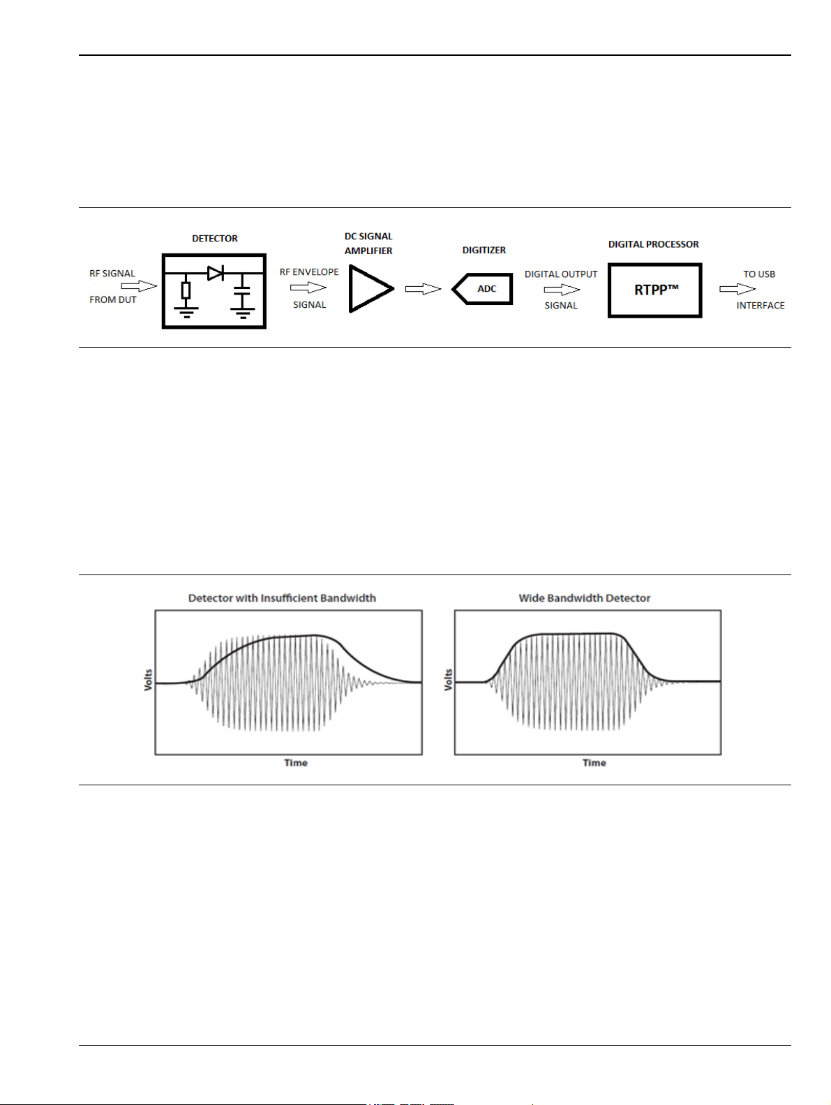
Figure 1-1 shows a block diagram of the peak power sensor.

Figure 1-1. MA244xxA Peak Power Sensors Block Diagram

The first and most critical stage of a peak power sensor is the detector, which removes the RF carrier signal
and outputs the amplitude of the modulating signal. The width of the detector’s video bandwidth dictates the
sensor’s ability to track the power envelope of the RF signal. The image on the left of Figure 1-2 shows how a
detector with insufficient bandwidth is unable to track the signal’s envelope effectively, affecting the accuracy
of the power measurement.

The image on the right shows sufficient video bandwidth to track the envelope accurately. The fast detectors
used in peak-power sensors are by their nature non-linear, so shaping procedures within the digital processor
must be used to linearize their response. When measuring instantaneous peak power, a high-sample rate is
important to ensure that no information is lost. The MA244xxA Peak Power Sensors have a sample rate of 100
MS/s, enabling capture and analysis of power versus time waveforms at a very high resolution.

Figure 1-2. Comparison of Bandwidth Detectors

MA244xxA UG PN: 10585-00033 Rev. C 1-3

1-5 Instrument Care and Preventive Maintenance General Information

1-5 Instrument Care and Preventive Maintenance

Instrument care and preventive maintenance consist of proper operation in a suitable environment, occasional
cleaning of the instrument, and inspecting and cleaning the RF connectors and all accessories before use.
Clean the instrument with a soft, lint-free cloth dampened with water or water and a mild cleaning solution.

Caution To avoid damaging the display or case, do not use solvents or abrasive cleaners.

Connector Care

Clean the RF connectors and center pins with a cotton swab dampened with denatured alcohol. Visually
inspect the connectors. The fingers of the N(f) connectors and the pins of the N(m) connectors should be
unbroken and uniform in appearance. If you are unsure whether the connectors are undamaged, gauge the
connectors to confirm that the dimensions are correct. Visually inspect the test port cable(s). The test port
cable should be uniform in appearance and not stretched, kinked, dented, or broken.

To prevent damage to your instrument, do not use pliers or a plain wrench to tighten the Type-N connectors.
The recommended torque is 12 lbf·in (1.35 N · m). The recommended torque for K connectors (2.92 mm) is
8 lbf·in (0.9 N·m). Inadequate torque settings can affect measurement accuracy. Over-tightening connectors
can damage the cable, the connector, the instrument, or all of these items.

Visually inspect connectors for general wear, cleanliness, and for damage such as bent pins or connector rings.
Repair or replace damaged connectors immediately. Dirty connectors can limit the accuracy of your
measurements. Damaged connectors can harm the instrument. Connection of cables carrying an electrostatic
potential, excess power, or excess voltage can damage the connector, the instrument, or both.

Connecting Procedure

1. Carefully align the connectors. The male connector center pin must slip concentrically into the contact
fingers of the female connector.

2. Align and push connectors straight together. Do not twist or screw them together. A slight resistance can
usually be felt as the center conductors mate.

3. To tighten, turn the connector nut, not the connector body. Major damage can occur to the center
conductor and to the outer conductor if the connector body is twisted.

4. If you use a torque wrench, initially tighten by hand so that approximately 1/8 turn or 45 degrees of
rotation remains for the final tightening with the torque wrench.

Relieve any side pressure on the connection (such as from long or heavy cables) in order to assure
consistent torque. Use an open-end wrench to keep the connector body from turning while tightening
with the torque wrench.

Do not over-torque the connector.

Disconnecting Procedure

1. If a wrench is needed, use an open-end wrench to keep the connector body from turning while loosening
with a second wrench.

2. Complete the disconnection by hand, turning only the connector nut.

3. Pull the connectors straight apart without twisting or bending.

1-4 PN: 10585-00033 Rev. C MA244xxA UG

General Information 1-6 Contacting Anritsu for Sales and Service

ESD Caution

The MA244xxA power sensors, like other high performance instruments, are susceptible to electrostatic
discharge (ESD) damage. Coaxial cables and antennas often build up a static charge, which (if allowed to
discharge by connecting directly to the instrument without discharging the static charge) may damage the
MA244xxA input circuitry. Instrument operators must be aware of the potential for ESD damage and take all
necessary precautions.

Operators should exercise practices outlined within industry standards such as JEDEC-625 (EIA-625),
MIL-HDBK-263, and MIL-STD-1686, which pertain to ESD and ESDS devices, equipment, and practices.
Because these apply to the MA244xxA power sensors, it is recommended that any static charges that may be
present be dissipated before making connection. It is important to remember that the operator may also carry
a static charge that can cause damage. Following the practices outlined in the above standards will ensure a
safe environment for both personnel and equipment.

1-6 Contacting Anritsu for Sales and Service

Customers having questions or equipment problems should visit this website and select the services in your
region: http://www.anritsu.com/contact-us.

MA244xxA UG PN: 10585-00033 Rev. C 1-5

1-6 Contacting Anritsu for Sales and Service General Information

1-6 PN: 10585-00033 Rev. C MA244xxA UG

Chapter 2 — Installation

1

2

6

5 4 3

2-1 Introduction

This chapter contains unpacking and repacking instructions, installation instructions for the software, and
power requirements for the sensors.

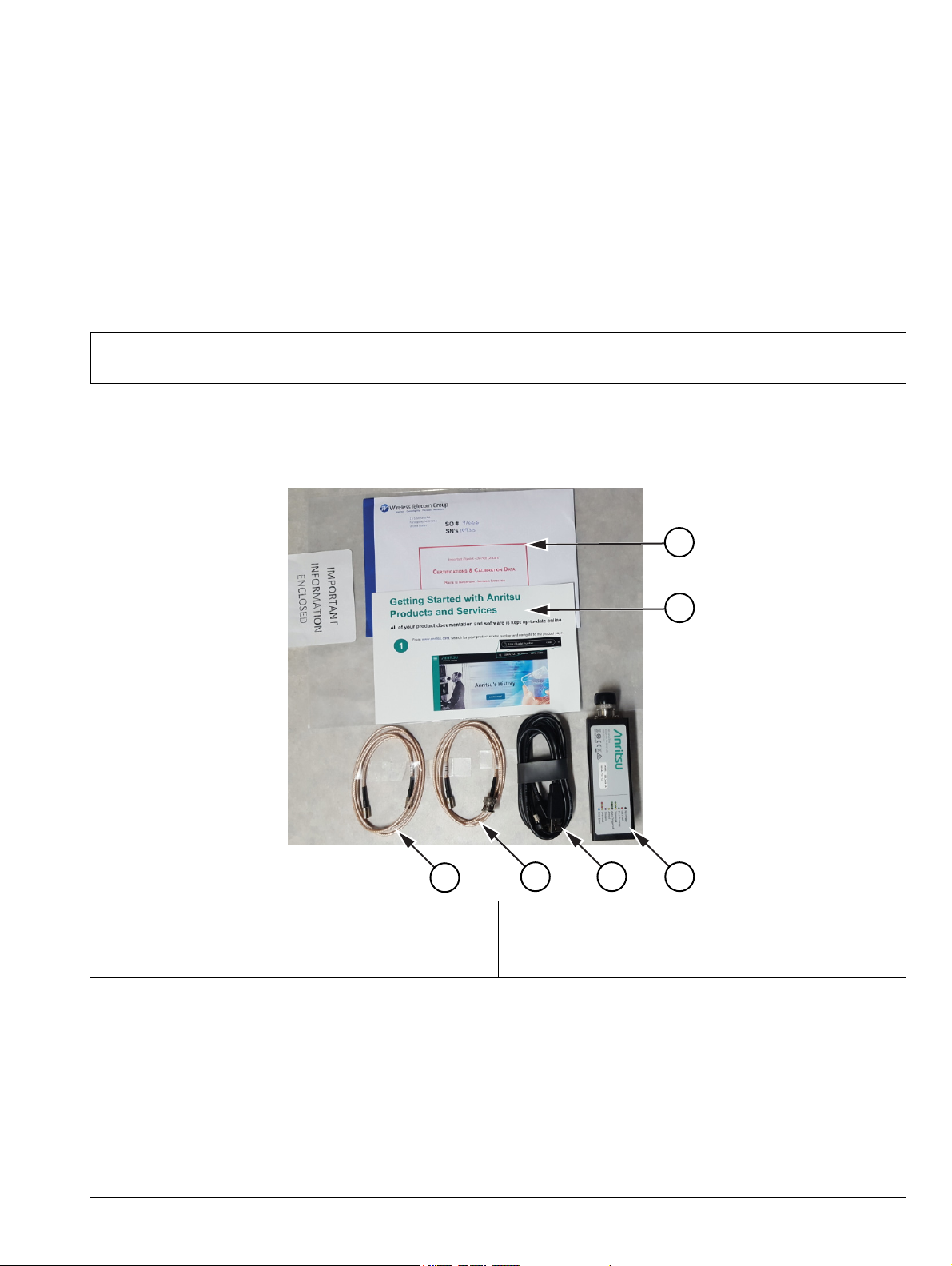
2-2 Unpacking

Caution

The MA244xxA Peak Power Sensors are shipped complete and are ready to use upon receipt. Verify the items
in your power sensor package as shown in Figure 2-1, If any of the items are missing or damaged, refer to
contact Anritsu Customer Service.

Follow all ESD (electro-static discharge) precautions and procedures when handling, connecting, or
disconnecting the MA244xxA Peak Power Sensors.

1. Calibration Certificate

2. Information Card

3. MA244xxA Power Sensor

Figure 2-1. MA244xxA Peak Power Sensors Kit

4. USB Type-A Cable (6 ft)

5. External Trigger Multi-I/O Cable (SMB to BNC)

6. Trigger Sync Cable (SMB to SMB)

2-3 Repacking

When repacking the sensor, use the original packing materials or equivalent.

MA244xxA UG PN: 10585-00033 Rev. C 2-1

2-4 Installing MA244xxA Software Installation

2-4 Installing MA244xxA Software

This section describes the installation and use of the MA244xxA USB Peak Power Sensor software. Before you
start, check your computer for compatibility against these minimum computer characteristics:

Caution

• Processor: 1.3 GHz or higher, recommended

• RAM: 512 MB (1 GB or more, recommended)

• Operating System:

• Hard-disk free space: 1.0 GB free space to install or run

• Display resolution: 800x600 (1280x1024 or higher, recommended)

• Interface: USB 2.0 high-speed

Installation Procedure

MA244xxA provides a PC User Interface for making Peak Power Measurements.

To install the MA244xxA Peak Power Analyzer software:

1. Download the latest MA244xxA USB Peak Power Sensor software from the Anritsu Website:

https://www.anritsu.com/en-us/test-measurement/support/downloads/software/dwl19784

2. Click Download

3. Select Run to start the installation.

4. Click through the installation screens. The installation creates a folder on the users PC that is located

here: C:\Program Files (x86)\MA24400A Peak Power Analyzer. Open the folder to launch
AnritsuPowerAnalyzer.exe. Once launched, the MA244xxA PC User Interface will appear as shown in

Figure 2-2.

Do not connect the MA244xxA Peak Power Sensors to your PC until you have installed the
MA244xxA Peak Power Analyzer software.

• Microsoft® Windows® 10

• Microsoft® Windows® 8 (32-bit and 64-bit)

• Microsoft® Windows® 7 (32-bit and 64-bit)

Figure 2-2. MA244xxA PC Interface Display

2-2 PN: 10585-00033 Rev. C MA244xxA UG

Chapter 3 — Getting Started

This chapter provides MA244xxA Peak Power Sensors basic connection and operation. For a detailed
functional description, see Chapter 4, “Operation."

3-1 MA244xxA Input Power Requirements

The MA244xxA Peak Power Sensors require 2.5 Watts at 5 Volts, this is supplied via a USB port. Therefore,
power sensor MUST be connected to a USB 2.0 compatible port that is able to supply 500 mA.

Usually a USB 2.0 port is capable of supplying 500 mA current through its port. When an

Note

3-2 Connecting the MA244xxA Peak Power Sensors

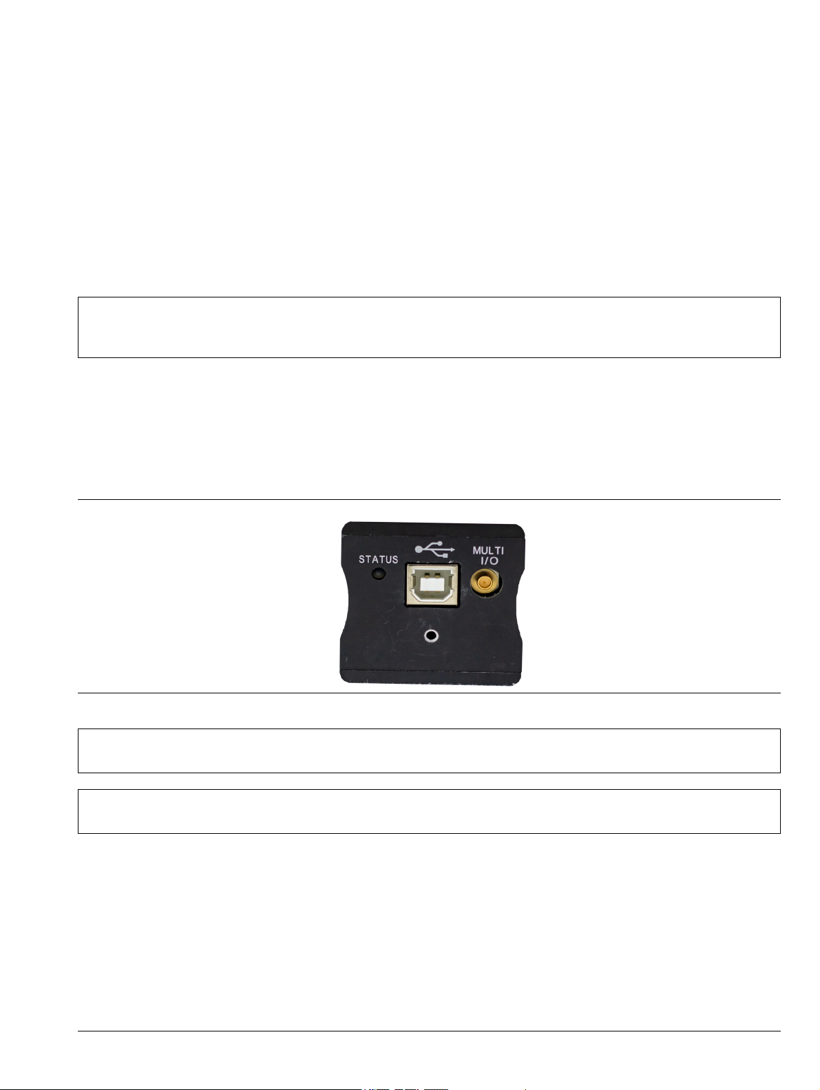
The rear panel of the MA244xxA Peak Power Sensors, shown in Figure 3-1, has two connectors and a status
LED. The larger connector is a USB Type B receptacle used to connect the MA244xxA Peak Power Sensors to
the host computer. The connector labeled MULTI I/O is an SMB plug and can serve as a trigger input, a status
output, or as a trigger-synchronizing interconnection when multiple MA244xxA Peak Power Sensors are used.

un-powered USB hub is used (sometimes the hub is internal), available current may need to be
shared between connected devices.

Figure 3-1. The Power Sensor Rear Panel

Note

Caution

To connect the sensor to the PC and to an RF source:

MA244xxA UG PN: 10585-00033 Rev. C 3-1

The MA244xxA Peak Power Analyzer software must be installed prior to connecting the sensor but
should not be started until the sensor is connected.

Follow all ESD (electrostatic discharge) precautions and procedures when handling, connecting, or
disconnecting the MA244xxA Peak Power Sensors.

3-1 MA244xxA Input Power Requirements Getting Started

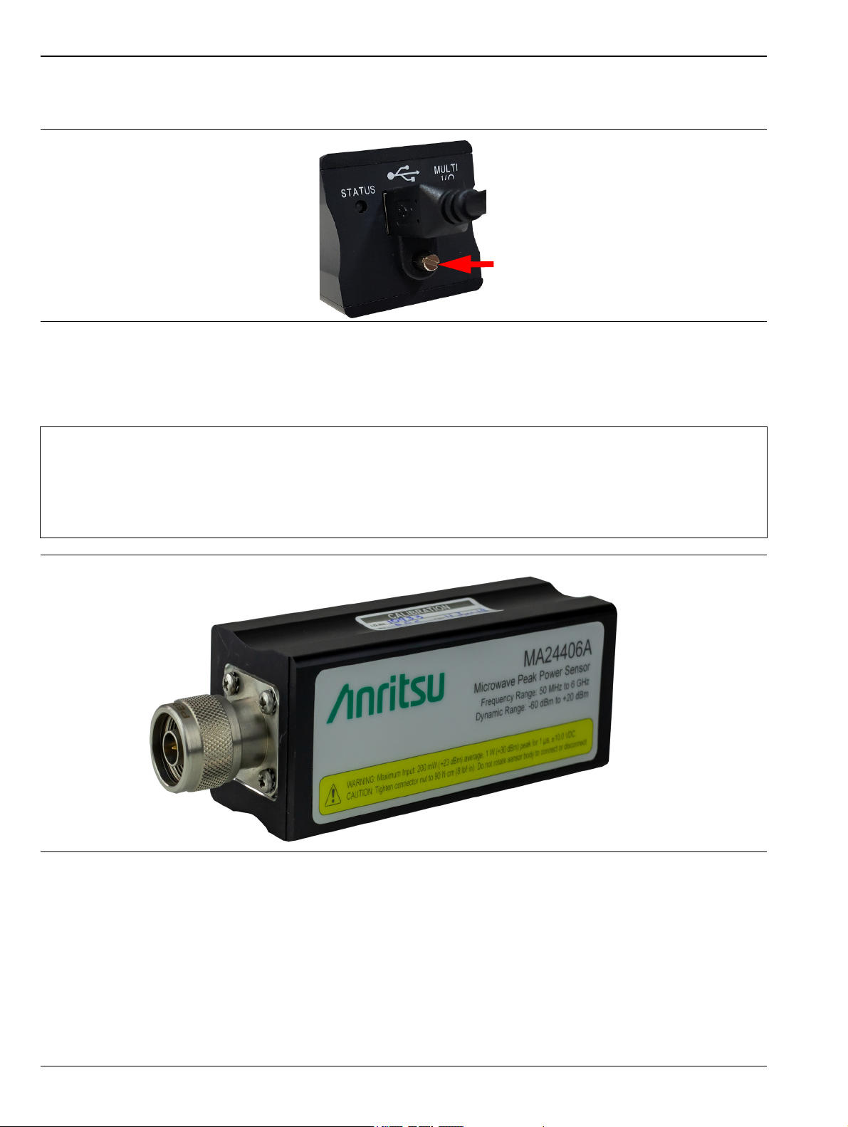
1. Connect the power sensor to your PC with the supplied USB cable. The cable should be secured
(hand-tight only) to the sensor using the captive screw on the USB plug. See Figure 3-2

Figure 3-2. Captive Screw for the USB Cable

2. Connect the MA244xxA Peak Power Sensors to the RF signal to be measured. All MA244xxA Peak
Power Sensors models are equipped with either a precision Type-N male RF connector (for applications
up to 20 GHz) or a precision 2.92 mm male RF connector (for applications up to 40 GHz).

Use the connecting and disconnecting procedures described in “Instrument Care and Preventive

Maintenance” on page 1-4.

Caution

Do not exceed the specified RF input power as specified on the front label. See Figure 3-3 for
location of this information.

Ensure that you do not apply any excessive forces to the sensor after it is connected.

Figure 3-3. MA24406A With N-Type Connector

3. Connect additional sensors according to your needs. See “Multichannel Operation” on page 4-29 for
connection schemes for multichannel situations.

Up to eight sensors can be connected to the MA244xxA Peak Power Analyzer.

4. Start the MA244xxA Peak Power Analyzer. Refer to “Starting the MA244xxA Peak Power Analyzer”.

3-2 PN: 10585-00033 Rev. C MA244xxA UG

Getting Started 3-3 Status LED Codes

No Power

Init Fault

Free Runing

Triggered

Auto Triggered

3-3 Status LED Codes

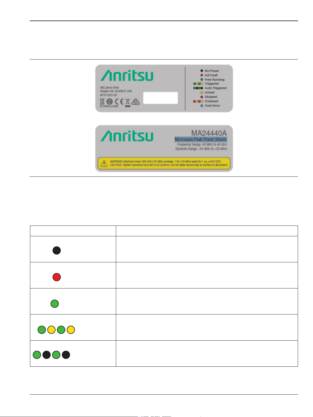
The rear panel shown in Figure 3-1 on page 3-1 includes a status LED. The color and flash pattern indicate the
sensor’s status as indicated on the label on the side panel shown in Figure 3-4.

Figure 3-4. Information Labels on the MA244xxA Peak Power Sensors

The information labels (see Figure 3-3 and Figure 3-4) on the MA244xxA Peak Power Sensors contain
information on the maximum input power levels and a description of the various status LED flash patterns.

Table 3-1. LED Status Indicators

Icon Description

No Power: No input power detected.

Init Fault: Initialize meter setting failed.

Free Running: Generating horizontal sweeps asynchronously, without

regard to trigger conditions.

Triggered: Indicates a preset triggered condition has occurred.

Auto Triggered: Automatically generates a trace if no trigger edges are

detected for a period of time.

MA244xxA UG PN: 10585-00033 Rev. C 3-3

3-4 Starting the MA244xxA Peak Power Analyzer Getting Started

Armed

Stopped

Overload

Cmd Error

Tab le 3- 1 . LED Status Indicators

Icon Description

Armed: Meter is armed and waiting for trigger event.

Stopped: Measurement Stopped.

Overload: Input power is too high. Reduce input power.

Cmd Error: Command Error return. Measurement is not valid.

3-4 Starting the MA244xxA Peak Power Analyzer

After you have installed the software and connected the power sensor to the PC, you are ready to make
measurements using the MA244xxA Peak Power Analyzer.

To start making measurements:

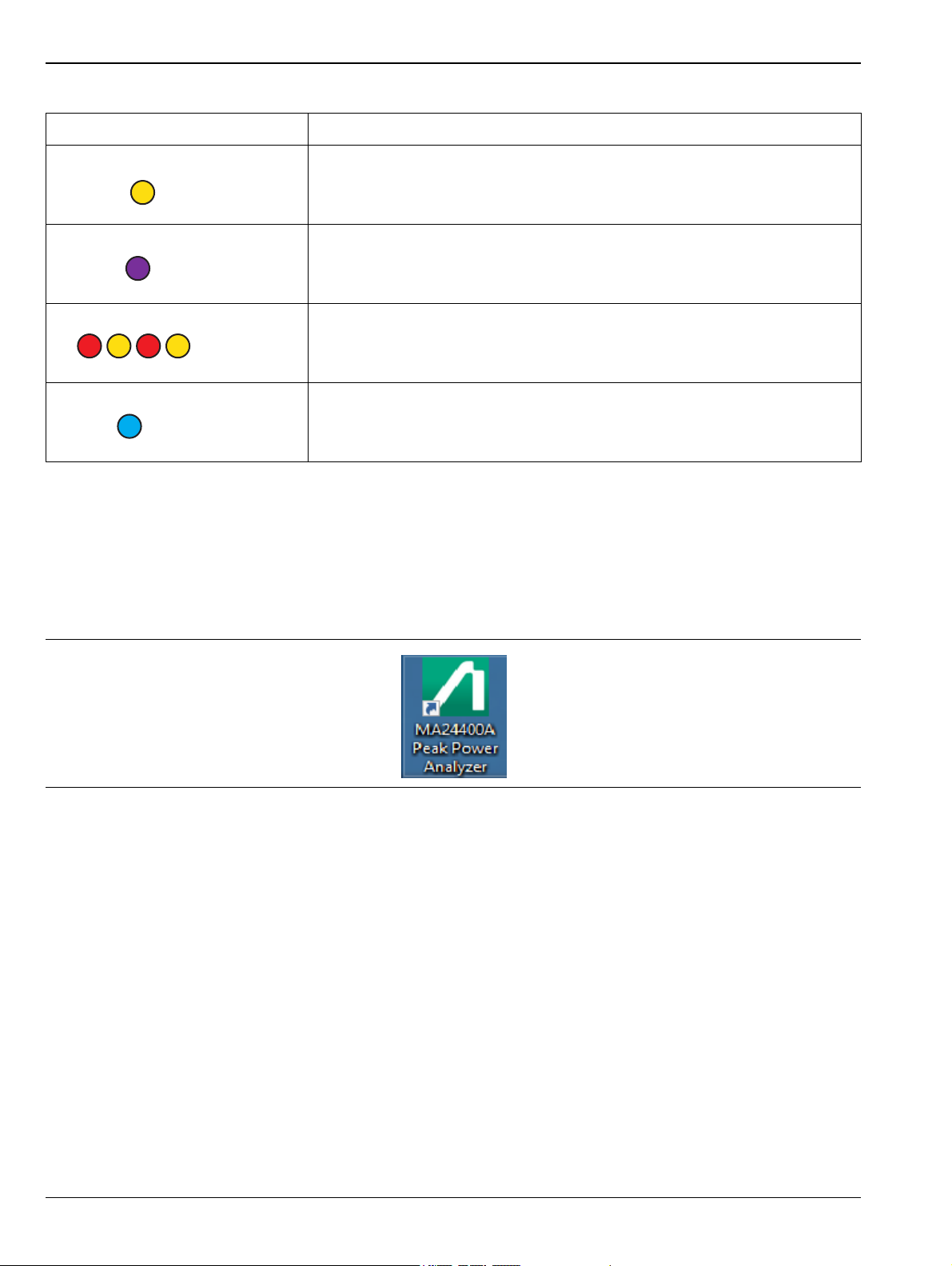
1. Start the MA244xxA Peak Power Analyzer by double-clicking the desktop icon.

Figure 3-5. MA244xxA Peak Power Analyzer Desktop Icon

A splash screen welcomes you to the application.

3-4 PN: 10585-00033 Rev. C MA244xxA UG

Getting Started 3-4 Starting the MA244xxA Peak Power Analyzer

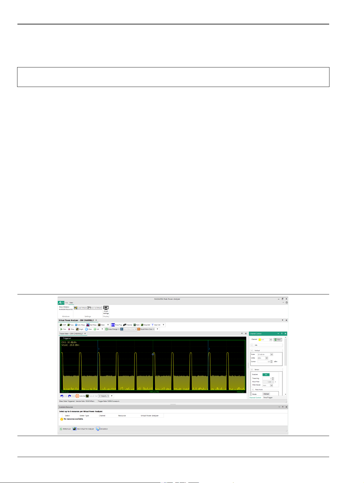
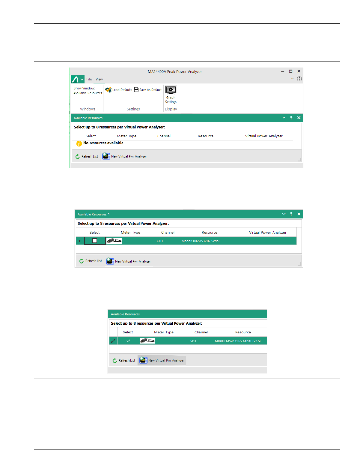
If no sensors are connected, the MA244xxA Peak Power Analyzer displays the No resources available
message as shown in Figure 3-6. If this is the case, close the analyzer, connect one or more sensors and
restart the analyzer.

Figure 3-6. No Resources View Available

With a sensor connected, the Available Resources window shows a list of the connected devices

Figure 3-7. Available Resources Box

2. In the Available Resources window, check select boxes for one or more connected sensors.

Figure 3-8. Selecting a Sensor from the Available Resources List

MA244xxA UG PN: 10585-00033 Rev. C 3-5

3-5 MA244xxA Peak Power Analyzer Basics Getting Started

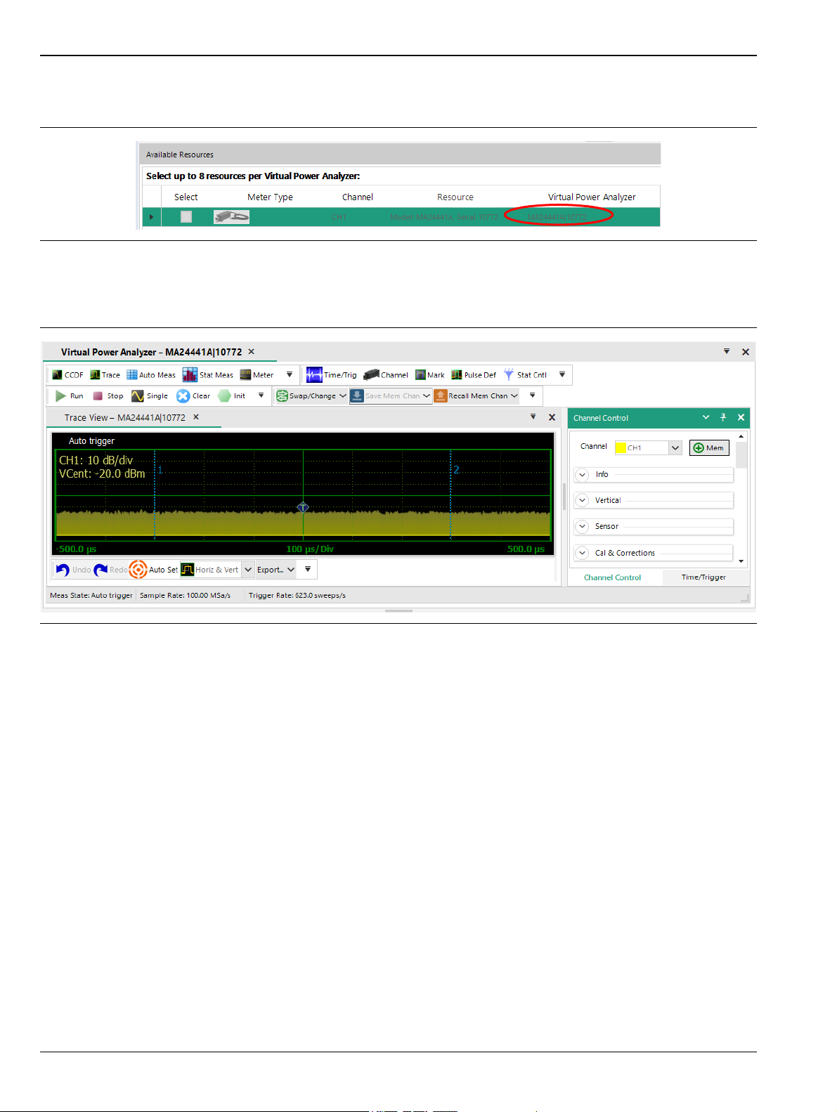
3. Click New Virtual Pwr Analyzer. This launches a new Virtual Power Analyzer instance containing trace
and control panels, and adds the Virtual Power Analyzer name to the Available Resource entries.

Figure 3-9. The Available Resources Box Shows Assigned Devices

4. If you have an RF signal connected to the USB sensor, the measured signal's waveform appears in the
trace window.

Figure 3-10. Initial View of the Virtual Power Analyzer

A Virtual Power Analyzer is analogous to a bench-top RF power analyzer with one or more sensors connected.
Time and trigger controls are typically common to all sensors within a MA244xxA Peak Power Analyzer, while
channel-specific controls are available for most other settings. This offers users the familiar, multi-channel
approach common to power meters and oscilloscopes.

When independent control of timebase-related settings is desired, you may open multiple MA244xxA Peak
Power Analyzer windows, each with their own sets of controls.

3-5 MA244xxA Peak Power Analyzer Basics

Dockable Windows

The MA244xxA Peak Power Analyzer uses dockable windows that allow you to arrange the various windows
into the configuration of your choice. You can drag a docked window by clicking its title bar. This action enables
them to move the window to a different docked position or undock it.

To dock tool windows:

1. Click and hold the title bar of the tool window you want to dock.

2. Start dragging the window.

Guide arrows appear pointing toward the four sides of the main window.

3-6 PN: 10585-00033 Rev. C MA244xxA UG

Getting Started 3-5 MA244xxA Peak Power Analyzer Basics

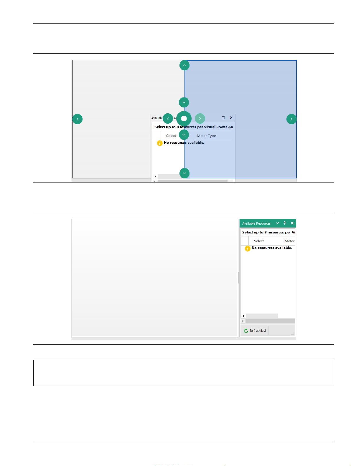
3. When the tool window you are dragging reaches the location where you want to dock it, move the pointer
over the corresponding portion of the guide diamond. The designated area is shaded blue.

Figure 3-11. Docking a Window

4. To dock the window in the position indicated, release the mouse button.

Figure 3-12. Docking a Window to the Right-side of the Main Window

Each of the tool windows may be positioned by dragging in any direction within the main window.

Note

Figure 3-11 on page 3-7 is one example; but you can rearrange tool windows as you prefer to see

them within the main software window or onto the desktop; Figure 3-13 shows this.

5. Docked windows can be overlapped. By selecting individual tabs, it is possible to resize and reposition
each tool window.

MA244xxA UG PN: 10585-00033 Rev. C 3-7

3-5 MA244xxA Peak Power Analyzer Basics Getting Started

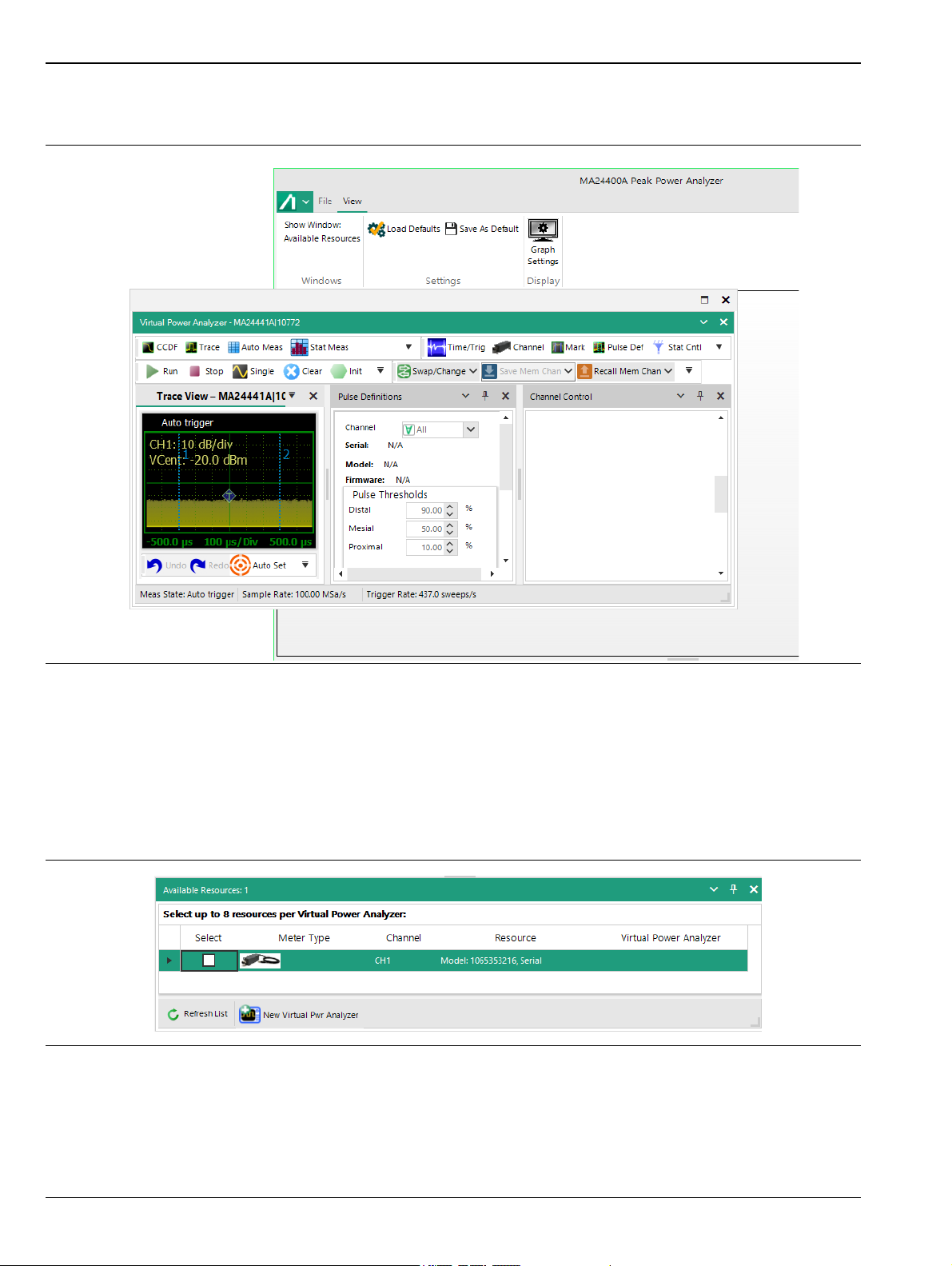
6. Docked windows can also be moved partially or completely out of the MA244xxA Peak Power Analyzer
main window.

Figure 3-13. Partial Window Repositioning

Available Resources Window

Sensors can be selected from the Available Resources window. A description for each connected resource
indicates the hardware version, model, and channel information, including alias. Users can select up to eight
resources per Virtual Power Analyzer instance. After selecting sensors, click New Virtual Pwr Analyzer and a
new Virtual Power Analyzer instance opens for those sensors with default configurations suitable for pulse
measurements.

Figure 3-14. Selecting a Sensor Using the Available Resources Box

3-8 PN: 10585-00033 Rev. C MA244xxA UG

Getting Started 3-5 MA244xxA Peak Power Analyzer Basics

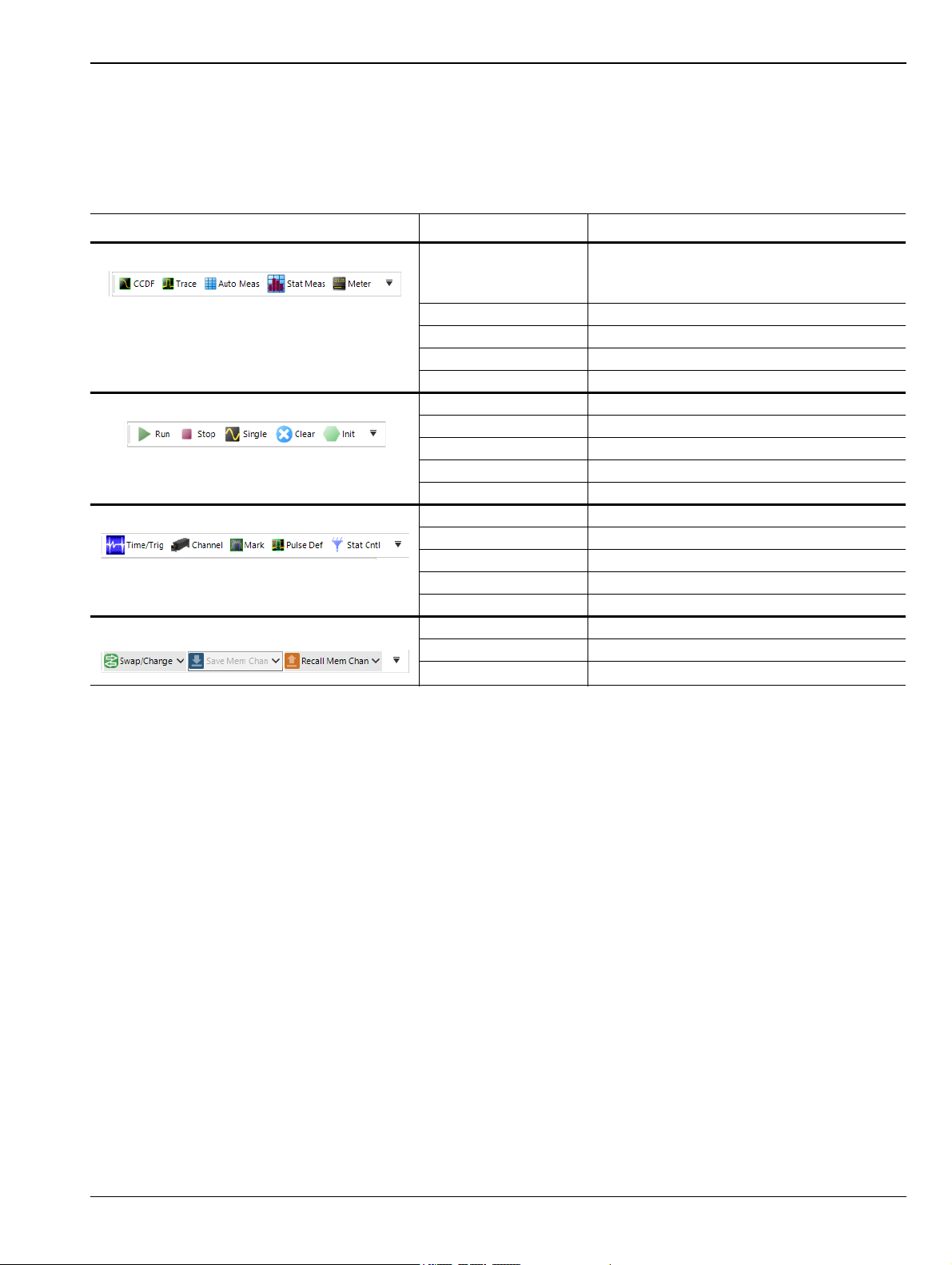
Virtual Power Analyzer Main Toolbar

Each Virtual Power Analyzer window displays a main toolbar at the top of its window which hosts shortcuts to
commonly used functions and measurement modes. The main toolbar is subdivided into smaller toolbars by
function; the order of tools in each toolbar may be customized or the groups may be dragged and dropped as
needed to provide more usable arrangements.

Toolbar Tool Description

Measurement Control CCDF Opens the CCDF window

(Complementary Cumulative Distribution

Function)
Trace Opens the trace window
Auto Meas Opens the auto measurement window
Statistical Meas Opens the stat measurement window
Meter Opens the meter view

Acquisition Control Run Starts a capture

Stop Stops a capture
Single Performs a single sweep
Clear Clears measurement buffer
Init Initializes meter settings

Control Windows Time/Trig Views time and trigger settings

Channel Views channel controls
Mark Opens marker control form
Pulse Def Opens pulse definition editor
Stat Cntl Opens stat mode control editor

Memory Channel

Swap/Change Swaps the USB power meter for a channel
Save Mem Channel Saves (archives) a memory channel
Recall Mem Channel Loads an archived memory channel

Figure 3-15. Main Toolbar Toolbars

MA244xxA UG PN: 10585-00033 Rev. C 3-9

3-5 MA244xxA Peak Power Analyzer Basics Getting Started

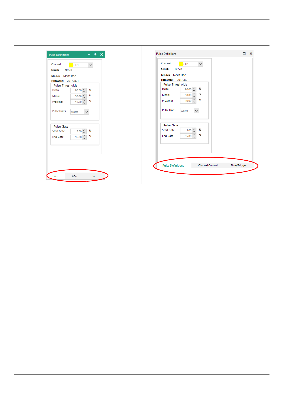
With each of these tools is associated a dialog; these are described in Chapter 4 in more detail. When several
are open simultaneously you can switch between them using the shortcuts at the bottom of the dialog.

Figure 3-16. Toolbar Shortcuts: Left View is Docked; Right View is Undocked.

3-10 PN: 10585-00033 Rev. C MA244xxA UG

Getting Started 3-5 MA244xxA Peak Power Analyzer Basics

Trace Group

Trigger Group

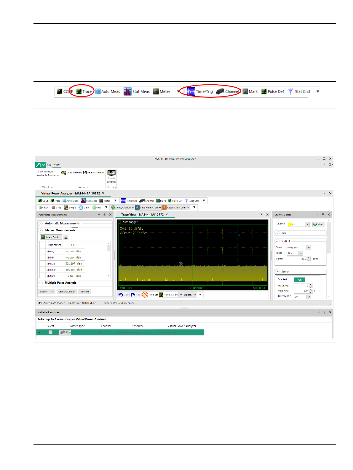
Trace View Window

To display a pulse measurement, select the Trace button from the Measurement toolbar. This is the default
view for a Virtual Power Analyzer instance.

The Channel and Time/Trig(ger) settings are related to pulse measurement can be selected from the Control
toolbar and can be applied to the measurement.

Figure 3-17. The Trace, Channel, and Time/Trigger Buttons

A Virtual Power Analyzer instance, in a configuration suitable for pulse measurements, is shown in

Figure 3-18. This shows a large trace window, automatic measurements, and a tabbed control box for time and

channel settings.

Figure 3-18. Main Application Window of the MA244xxA Peak Power Analyzer

The Virtual Power Analyzer allows you to directly enter numeric values for most settings in the Channel
Control and Time/Trigger windows. For many of the controls, additional methods such as increment/decrement
or preset buttons are available.

MA244xxA UG PN: 10585-00033 Rev. C 3-11

3-5 MA244xxA Peak Power Analyzer Basics Getting Started

Virtual Power Analyzer Lower Toolbar

Trace Pan and Zoom

The mouse can be used to select a zoom area to view detail in an area of interest on the displayed waveform.
The highlighted dragged rectangular area indicates the minimum area that will be shown when the zoom
operation completes.

Horizontal pan or zoom adjusts the timebase (within preset values) and the trigger delay to highlight an area
of interest without vertical rescaling.

You can also directly pan or zoom to waveform areas of interest by selecting any option from the lower toolbar
of the trace window. Available options for zoom/pan control are: Horizontal & Vertical, Horizontal, Pan and
None.

Clicking the Trace View display, dragging a zoom box, and releasing the mouse button results in the trace being
expanded to show the area outlined by the zoom indicators.

AutoSet

The Auto Set button tries to configure level scaling, trigger level, and timing for a best-fit display based upon
amplitude and timing of the applied signal. All other parameters are set to defaults. If the Auto Set process
fails, all settings are left untouched.

You can undo or redo an action with the undo and redo buttons.

Trace Data Export

Any trace window can be exported and saved or printed as a PDF or CSV document by selecting PDF or CSV
from the Export drop-down menu. An exported trace file can easily be imported into a spreadsheet or other
report file or documentation.

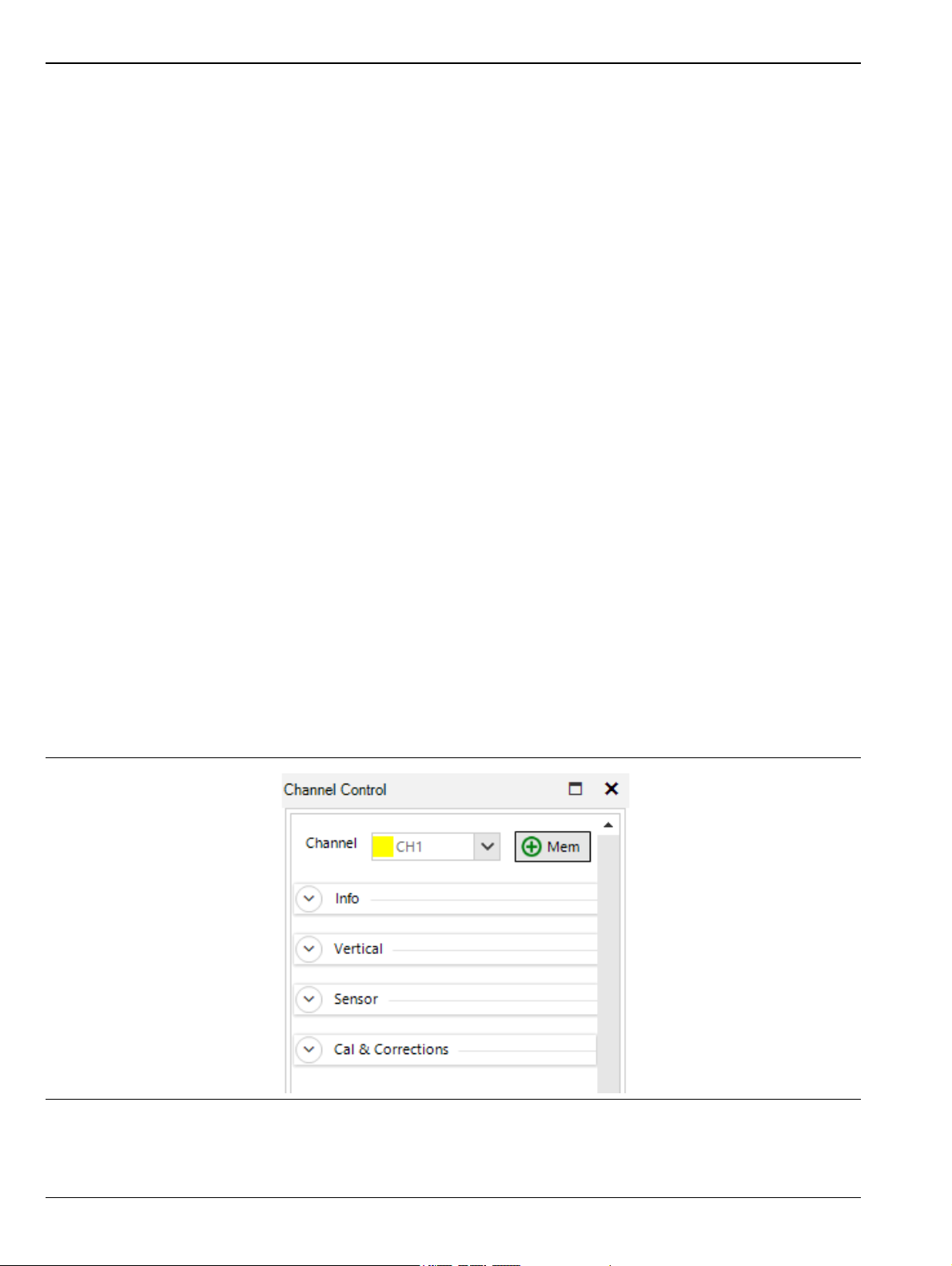
Channel Control Window

Select the Channel button of the Trigger group and a dockable sidebar appears, by default, on the right-hand
side of the main application window. This allows you to change all the related settings that control one or more
sensor channels. The Channel Control is defined by these parameters.

Figure 3-19. Channel Control Dialog

3-12 PN: 10585-00033 Rev. C MA244xxA UG

Getting Started 3-5 MA244xxA Peak Power Analyzer Basics

Channel

Select one channel to update from the drop-down list or select All channels (available only with multiple
channels) to simultaneously update all measurement channels (up to 8) for most settings.

Memory Pull-down

You can select the stored memory channels.

Info Group

Serial: Displays the serial number of the sensor.

Model: Displays the model number of the sensor.

Firmware: Displays the date of the firmware version.

FPGA: Displays the FPGA version.

Mark Control: Brings up the Mark Control dialog.

Pulse Definition: Brings up the Pulse Definition dialog.

Vertical Group

Scale: Sets vertical amplitude scaling and centering of the displayed waveform. These settings

affect only the Trace display.

Units: Selects dBm, Watts, or Volts measurement units. Selection affects displayed text,

measurements, and trace.

Center: The center frequency for the display.

Sensor Group

Sensor Enabled: Enable or disable individual connected sensors.

Trace Avg: Sets number of acquired sweeps averaged together for displayed trace in pulse/triggered

modes. Useful for noisy signals.

Mod Filter: Sets the modulation filter integration time.

Filter Mode: Sets manual or automatic filter integration time window for measurements in modulated

(non-triggered) acquisition modes.

Video BW: Selects sensor video bandwidth, high or low.

Frequency: Sets measurement frequency for the applied RF signal.

Peak Hold Group

Mode: Sets the mode of the sensor to either manual or tracking.

Decay Count: Sets peak hold duration (# of sweeps).

Cal&Corrections Group

Offset: Compensates reading for external gain/loss.

Zero and Fixed Cal : Performs sensor zeroing or fixed calibration by selecting each specific button.

Clear User Cal: Clears any user calibration for the sensor selected (refer to “Channel” on page 3-13).

Fixed Cal: Performs a calibration at 0 dBm at the currently set frequency.

MA244xxA UG PN: 10585-00033 Rev. C 3-13

3-5 MA244xxA Peak Power Analyzer Basics Getting Started

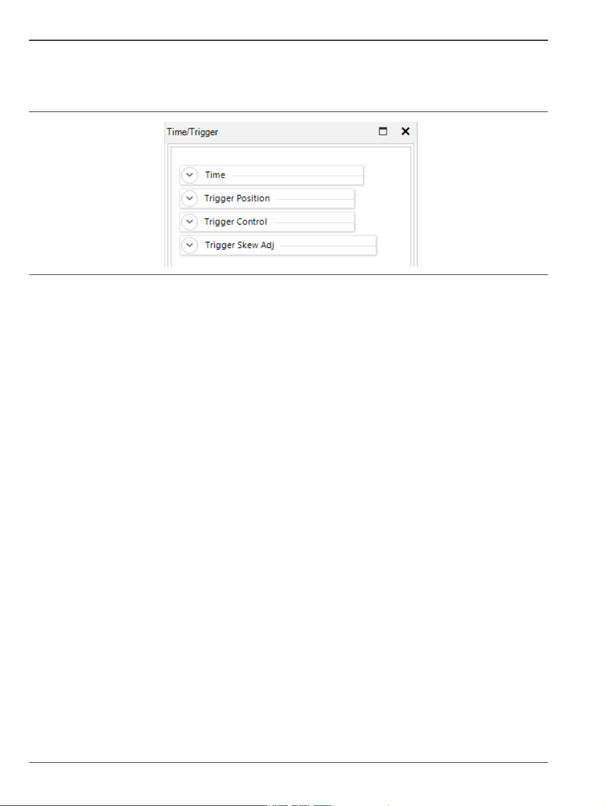
Time / Trigger Settings Window

Click the Time/Trig button of the Trigger group to customize all related settings for both timebase and trigger of
a pulse signal. Refer “Time/Trigger Control Window” on page 4-5 for details.

Figure 3-20. Time and Trigger Dialog

Time

Timebase: Acquisition time in seconds per division. The power sensors use a fixed grid of 10

divisions for the sweep extents. Settings are in a 1-2-5 sequence. Consult series
specifications for timebase range.

Trigger: Delay The trigger delay can be adjusted by manually entering a numerical value into the

field or using the up-down arrow keys. Refer to “Time Control” on page 4-6.

Trigger Position

The trigger position can be changed by entering numerical values into the Divisions field, clicking the
scroll arrows, dragging the slide control, or by clicking the L/M/R (Left/Middle/Right) indicators. Refer to

“Trigger Position Control” on page 4-7.

Trigger Control

Source: Several trigger modes are available for each trigger source under Trigger Control section.

Multiple trigger sources are available under the drop-down list including both Internal
and External selection.

Mode: Select Normal, Auto, AutoLevel or Free run.

Level: Sets trigger level when trigger source is INT and trigger mode is Auto or Normal.

Slope: Selects rising- or falling-edge triggering.

Holdoff: Sets trigger holdoff time.

Holdoff Mode : Selects between Normal or Gap.

Trigger Skew

Adjustment: Adjusts the skew for internal trigger with master trigger output, and also external and

slave triggers. Skew adjustments allow you to calibrate out-trigger delay between sensors
so the you can measure the propagation delay of the DUT from input to output. Manual
skew adjustments can be made by entering the skew value in the numeric entry field.
The button to the right of each skew adjustment is the Auto-Skew, which allows
automatic adjustment of the skew. Refer to“Trigger Skew Adj(ust)” on page 4-9.

3-14 PN: 10585-00033 Rev. C MA244xxA UG

Getting Started 3-5 MA244xxA Peak Power Analyzer Basics

Marker Settings Window

Click Mark of the Control Windows toolbar to control settings for time markers and reference lines of a pulse
signal. refer to “Marker Settings Window” on page 4-20.

Figure 3-21. Marker Settings Window

Markers: Allow you to change both Marker 1 and Marker 2 time positions by using either arrow

keys or entering numerical values into the fields. It also displays the time delta value
between the two markers. You may also drag the markers in the active window and their
values will be reflected in this window.

Reference Lines: Also known as Horizontal Markers, they can be enabled by selecting the On/Off button for

each individual channel. After they are enabled, users may select several options for
automatic amplitude tracking from the Tracking drop-down list: Off, Markers,
TopBottom, DistalMesial and DistalProximal. Two reference lines can be set by using
up/down arrow keys. Horizontal markers are useful to determine the difference with
regard to loss.

MA244xxA UG PN: 10585-00033 Rev. C 3-15

3-5 MA244xxA Peak Power Analyzer Basics Getting Started

Pulse Definitions Window

Click Pulse Def of the Trigger group to access settings for the pulse definitions. Refer to “Pulse Definitions

Window” on page 4-19.

Figure 3-22. Pulse Definitions Menu

Channel: The channel to which the definitions will be applied.

Serial: The serial number of the unit. (Not applicable when all channels are selected.)

Model: The model number of the unit. (Not applicable when all channels are selected.)

Firmware: The version number of the installed firmware on the unit. (Not applicable when all

channels are selected.)

Pulse Thresholds:

Pulse definition settings allow you to define distal, mesial, and proximal values for pulse thresholds. You
may change the pulse unit between watts and volts.

Pulse Gate

Pulse Start and End Gates can be changed both numerically and by using the up/down arrow keys. It is
not necessary that the two of them total to 100%.

Chapter 5, “Making Measurements” contains a detailed description of the Pulse Threshold level and the pulse

measurement process.

3-16 PN: 10585-00033 Rev. C MA244xxA UG

Getting Started 3-5 MA244xxA Peak Power Analyzer Basics

Stat Mode Control Window

Click Stat Cntl of the Trigger group to access settings for the pulse definitions. Refer to “Statistical Mode

Control Window” on page 4-23.

Figure 3-23. Pulse Definitions Menu

Capture: Set to On to capture the stat mode.

Reset: Click to reset all the parameters.

Te rm Ac t io n : The action to take upon termination: Decimate, Restart, and Stop.

Term Count (Msa): Type or use the arrow buttons to enter a sample limit.

Terminal Time (s): The time in seconds for the sample period to end.

Horiz Offset (dB): Use the up-down arrow buttons to modify the amount of offset.

Horiz Scale: Choose the scale from six fixed values from 0.1dB to 5.0dB.

Cursor Type: Choose between percent (%) and power.

Cursor Pos (%): The position of the cursor in Type units.

Gating: Choose between Freerun and Markers.

Mark Cntrl: Opens the Marker Settings dialog.

MA244xxA UG PN: 10585-00033 Rev. C 3-17

3-5 MA244xxA Peak Power Analyzer Basics Getting Started

Automatic Measurements Window

Select the Auto Meas button to display three tabulated fields with lists of parameters for Multiple Pulse
Measurements, Automatic Measurements, and Marker Measurements. Figure 3-21 is an example screenshot
for Automatic Measurements displayed for a typical pulse measurement. Refer to “Automatic Measurements

Display” on page 4-15

Figure 3-24. Automatic Measurements Window: Collapsed View

All parameters are customizable and may be edited or deleted from these lists. A part of or the whole table may
be copied and pasted into a spreadsheet. Adding screenshots from the Export>PDF you make any custom
report file along. Export>CSV exports all the parameters from these lists to a CSV file.

To add a row to any table click on the table icon or Click here to add a new row. You may select from any of the
parameters in the drop-down list. Generally, this feature is used to replace any row that was deleted.

Figure 3-25. Selecting Automatic Parameters

Click Restore to restore all the factory default values to the parameter in the lists.

3-18 PN: 10585-00033 Rev. C MA244xxA UG

Getting Started 3-5 MA244xxA Peak Power Analyzer Basics

Customize Field Parameters

All field parameters under automatic measurement are customizable. They can be edited or deleted from the
list by selecting individual parameters with the right mouse button. Right-click a parameter to access its Edit
pop-up.

Figure 3-26. Pulse Measurement Pop-up

Export or Copy Field Parameters

The whole or partial automatic table or field can be copied and pasted into any spreadsheet or document.
Control+click those rows needed to make a custom report, and include screenshots captured by the application.

Figure 3-27. Select Multiple Parameters and Right-click to Copy

MA244xxA UG PN: 10585-00033 Rev. C 3-19

3-5 MA244xxA Peak Power Analyzer Basics Getting Started

Display (Graph) Settings Window

Select Graph Settings from the window toolbar to customize data and trace colors for each measurement
channel, and enable or disable trace display features such as Average, Envelope, Maximum, Minimum, and
Persistence.

Figure 3-28. Graph Setting Icon

It is also possible to adjust marker color, background, grid colors, and more under Graph Colors section of the
display settings.

Figure 3-29. Display Settings

3-20 PN: 10585-00033 Rev. C MA244xxA UG

Getting Started 3-5 MA244xxA Peak Power Analyzer Basics

CCDF View Window

For statistical measurements, select the CCDF (Complementary Cumulative Distribution Function) icon from
menu bar to view a CCDF graph. The sidebar on the CCDF screen allows adjustment of horizontal scale,
horizontal offset, cursor type, cursor position, and dB offset. You can also enable/disable capture or reset the
statistical data acquisition.

Figure 3-30. CCDF Graph

MA244xxA UG PN: 10585-00033 Rev. C 3-21

3-5 MA244xxA Peak Power Analyzer Basics Getting Started

Statistical Measurements Window

Click the Stat Meas button to display a tabulated list of statistical measurements. Figure 3-31 is an example
parameters text display for statistical measurements.

Figure 3-31. Statistical Measurements Window

This data can also be exported by holding Shift and pressing the up or down arrow keys until all the rows
needed are selected. Right-click on any of the selected rows and click Copy.

Figure 3-32. Exporting Data

3-22 PN: 10585-00033 Rev. C MA244xxA UG

Chapter 4 — Operation

4-1 Introduction

This chapter presents the procedures for using the MA244xxA Peak Power Analyzer to operate the MA244xxA
Peak Power Sensors. All the display windows that control the sensors are illustrated and accompanied by
instructions for each control in the window.

The MA244xxA Peak Power Analyzer is a Windows-based software program that provides immediate RF
power measurements from MA244xxA Peak Power Sensors without the need for programming on your
Windows OS-based computer. RF power measurements from the power sensor can be displayed on your
computer or can be integrated into a test system using an Application Program Interface (API).

This section of the manual requires that the MA244xxA Peak Power Analyzer is installed on a

Note

4-2 The Trace View Display

The Trace View shown in Figure 4-1, “Horizontal and Vertical Zoom on a Trace” is the default view when a
Virtual Power Analyzer is first opened. It displays a trace of power versus time. The readout in the upper left
corner shows the channel number of the trace, the vertical scale factor, and the vertical center. In Figure 4-1,
CH1 is displayed with a vertical scale of 10 dB/div(ision) and a vertical center of –20 dBm.

• The horizontal scale of the trace in the Trace View window is shown at the bottom of the grid. At the
center of the horizontal axis is the horizontal scale factor. Numbers at the right and left ends of the
horizontal axis show the trace start and end times relative to the trigger.

• The two vertical blue lines labeled 1 and 2 are markers used for measurements of the displayed signals.
Refer to “Marker Settings Window” on page 4-20.

• The bar at the bottom of the Trace View window provides useful tools that can be used to optimize the
trace display and archive the trace(s):

computer using the instructions provided in Chapter 2, “Installation” and that one or more sensors
are connected according to instructions provided in Chapter 3, “Getting Started”.

• The Export button is used to export any trace window as a PDF or CSV document. These exported
trace files can be used for a report or document.

• The Undo and Redo buttons work in conjunction with the display expansion (zoom) function to
remove (Undo) and restore (Redo) changes in display scaling.

• Autoset provides an automatic setup of the trace display scaling that optimizes the trace view in
the Trace View window.

• The pull-down menu selects the zoom mode from these options:

• Horiz(ontal) & Vert(ical), refer to “Trace Zoom: Horizontal and Vertical”

• Horizontal, refer to “Trace Zoom: Horizontal Only” on page 4-2

• Pan allows you to click and drag the trace either horizontally or vertically. You may also

drag the trace symbol to adjust the position of the trace.

• None prevents all zoom and pan actions.

MA244xxA UG PN: 10585-00033 Rev. C 4-1

4-2 The Trace View Display Operation

Trace Zoom: Horizontal and Vertical

The analyzer has a trace-zoom feature which lets you to drag a rectangular box (like the one shown in

Figure 4-1) around the trace to zoom onto a special area of the displayed waveform. The rectangular area

indicates the area that is enlarged when the mouse button is released. The zoom area is constrained to the
preset timebase settings and trigger Vernier limits. Note in Figure 4-1 that the zoom horizontal scale changes
from 10 µs/div to 1 µs/div (the nearest available fixed timebase setting). Vertical scaling is similarly
constrained.

Figure 4-1. Horizontal and Vertical Zoom on a Trace

Trace Zoom: Horizontal Only

Horizontal-only display expansion (zoom) is accomplished by clicking on the trace view and dragging the mouse
horizontally. A shaded box outlines the area to be expanded. Releasing the mouse button rescales the trace.

Figure 4-2. Horizontal Zoom

4-2 PN: 10585-00033 Rev. C MA244xxA UG

Operation 4-2 The Trace View Display

Formatting Trace View Display Settings

In the upper left-hand corner, click View (next to File) and then click the Graph Settings icon. This opens the
Display Settings popup as shown in Figure 4-3.

Figure 4-3. The Display Settings Popup

The Display Settings popup is used to configure the Graph View. The elements to be displayed can be chosen
and their colors may be selected, along with the background color.

The upper section of the Display Settings, labeled Trace, controls the configuration of the selected trace. There
can be a maximum of eight traces. The configuration of each trace includes the trace color, the choice of five
viewable trace attributes, and the trace refresh time. Trace attributes include graphical view of the average
value, envelope, maximums, minimums, and persistence (trace history). The defaults are Show Avg and Show

Envelope. Each of the selected elements is overlaid on the trace.

The sensor acquires all three traces (average, min and max) when required for a trace. These are
used for several of the marker measurements, such as interval, peak-to-average, and others. The
sensor also tracks Min and Max (highest maximum trace and lowest minimum trace points) as well

Note

as MinF and MaxF (minimum and maximum filtered) which are the highest and lowest points on the
average trace. The former measurements are useful for looking at modulation, while the latter are
most useful for seeing systematic peaks and dips (for example, ringing) of a repetitive waveform with
the noise reduced.

A check box for Disable HW Acceleration can be checked if the computer does not have a monitor or graphics
card or if it is operated remotely using Remote Desktop.

Note This change takes effect the next time a trace window is opened.

MA244xxA UG PN: 10585-00033 Rev. C 4-3

4-2 The Trace View Display Operation

The lower section of the Display Settings popup provides controls for color choices for trace grid, border, and
background. Markers, axis label, and crosshair color selections are also included. Color choices are made by
clicking on the ellipsis symbol (…) adjacent to each element. This brings up the Color Dialog palette used to set
the desired color for the element

The Main Toolbar

The MA244xxA Peak Power Analyzer always displays the Main Toolbar at the top of the main program
window and contains shortcuts to commonly used functions and measurements. The Main Toolbar can be
customized as discussed below. Figure 4-4 shows the Main Toolbar:

Figure 4-4. The Main Toolbar

The Main toolbar contains three sections. The group of shortcuts on the left, including CCDF, Trace, Auto
Meas (Measurement) and Stat Meas (Statistical Measurement) comprise the Measurement Windows toolbar
and bring up trace display or measurement panels. The middle group with Time/Trig (Trigger), Channel,
Mark, Pulse Def (Definitions) and Stat Cntl (Statistical Control) are the Control Windows toolbar. They cause
setup and control windows to be displayed. The right-most group including Run, Stop, Single, Clear, and Init
(Initialize) are the Acquisition Control toolbar and affect the state of the acquisition.

Any of the toolbars may be separated from the Main Toolbar and re-positioned by clicking on the ellipsis
symbol at the left end of any of the groups and dragging the toolbar.

The drop-down menu bar on the right of each section allows you to edit the tools bar by adding or removing any
of the items under the Items tab. The toolbars tab allows you to show or hide the toolbars.

The Acquisition Control Toolbar

The buttons on this toolbar control the state of the acquisition:

Run: Starts the measurement acquisition and allows it to run continuously until stopped.

Stop: Stops the measurement acquisition.

Single: Starts a single measurement acquisition and then stops.

Clear: Erases the acquired data trace. Useful when clearing single or averaged acquisitions.

Init: Initializes or resets all settings for the active Virtual Power Meter to default values.

The Measurement Control Toolbar

The buttons on this toolbar create Trace View and CCDF Graph displays as well as the automated power
measurement and statistical Measurement tabular display windows:

CCDF: This button turns on the complementary cumulative distribution function (CCDF)

display. If the CCDF display is already opened but hidden behind the Trace View display,
clicking this button brings the CCDF trace to the foreground. Refer to “Statistical CCDF

Graph Display” on page 4-22.

Trace: This button turns on the Trace View trace that displays power versus time. Refer to “The

Trace View Display” on page 4-1.

Auto Meas: This button opens Automatic Measurement windows showing the automatic Pulse and

Marker Measurements tables. Refer to “Automatic Measurements Display” on page 4-15.

Stat Meas: This button opens the Statistical Measurements window displaying the measurements

associated with the CCDF Graph. Refer to “Statistical Measurements Display”

on page 4-24

4-4 PN: 10585-00033 Rev. C MA244xxA UG

Operation 4-2 The Trace View Display

The Control Windows Toolbar

The buttons on this toolbar control the setup windows for the acquisition, and measurement functions.

Time/Trig: This button displays the Time/Trigger control windows. Refer to “Time/Trigger Control

Window” on page 4-5.

Channel: This button brings up the Channel Control Window, allowing control of the vertical range

and offset as well as sensor-related settings. Refer to “Channel Control Window”

on page 4-10.

Mark: This button causes the Marker Settings window to be displayed. Marker and reference

lines can be controlled from here. Refer to “Marker Settings Window” on page 4-20.

Pulse Def: This button displays the Pulse Definitions window controlling the pulse measurement

thresholds, units, and gating. Refer to “Pulse Definitions Window” on page 4-19.

Stat Cntl: This button brings up the Stat Mode Control window with scaling and population control

for the CCDF display. Refer to “Statistical Mode Control Window” on page 4-23.

Memory Channel Toolbar

The Memory Channel is a reference trace that appears on the Trace View when Mem+ is enabled. The Memory
Channel toolbar contains Swap/Change, Save Mem(ory) Chan(nel), and Upload Mem(ory) Chan(nel) options, and
these control the sensor connection source and the saving and recalling Mem(ory) traces.

Swap/Change: Allows you to change sensors for a particular session if more than one are connected.

Save Mem Chan: Saves the current memory channel archive to a user-selected folder on the computer.

Recall Mem Chan: Recalls a stored memory channel archive to the Memory Channel Trace on the Trace

View.

Time/Trigger Control Window

Pressing the Time/Trig button icon the Control Windows toolbar brings up the Time/Trigger control window.

Figure 4-5. The Time/Trigger Control Window

This window has these sections: Time (time base and delay), Trigger Position, Trigger Control, and Trigger
Skew Adj(ust). Any of these sections can be opened or collapsed by clicking the up/down arrow buttons to the
left of the section title.

MA244xxA UG PN: 10585-00033 Rev. C 4-5

4-2 The Trace View Display Operation

Time Control

These settings affect the horizontal scaling of the acquired waveform.

Figure 4-6. Time Control Settings

Timebase: Controls the timebase or horizontal scale of the acquisition and is noted on the horizontal

axis label of the Trace View. The Timebase pull-down menu permits selection of fixed
timebase ranges from 5 ns/div to 50 ms/div (sensor series dependent) in a 1-2-5
progression.

Click the icon to reset the trigger delay to zero seconds.

Trig(ger) Delay: This setting can be adjusted either manually, by entering a numerical value into the

field, or by using the up-down arrow keys.

The trigger delay time is set in seconds with respect to the trigger. Positive values mean
that the trace display shows a time interval after the trigger event. This positions the
trigger event to the left of the trigger point on the display, and is useful for viewing
events during a pulse, or some fixed-delay time after the rising edge trigger. Negative
trigger delay means that the trace display shows a time interval before the trigger event,
and is useful for looking at events preceding the trigger edge.

Pressing the '0' button to the right of the trigger delay entry field resets the trigger delay
to zero.

The range of trigger delay times is dependent on the timebase setting and is summarized
in Table 4-1. Note the range also depends upon the trigger position.

Tab le 4- 1 . Trigger Delay Summary

Timebase Setting Trigger Delay Range

5 ns/div to 10 us/div –1.26 ms to 100 ms

20 us/div –1.26 ms to 200 ms

50 us/ div –5.04 ms to 200 ms

100 us/ div –6.3 ms to 500 ms

200 us/div –12.6 ms to 1

500 us/div –31.5 ms to 1 s

1 ms/div –63 ms to 1 s

2 ms/div to 10 ms/div –126 ms to 1 s

20 ms/div –252 ms to 1 s

50 ms/div –628 ms to 1 s

4-6 PN: 10585-00033 Rev. C MA244xxA UG

Operation 4-2 The Trace View Display

Trigger delay ranges in Table4-1 onpage4-6 are for the trigger position set to 0 divisions (Left). If

Note

trigger delay and position settings result in a pretrigger capture interval greater than 1.26 ms, the
sensor automatically reduces the sample rate to avoid overflowing its pretrigger memory.

Trigger Position Control

This setting affects the position of the acquired waveform.

Figure 4-7. Trigger Position Setting

Trigger Position: This control sets the location of the trigger point on the acquired trace waveform. It can

be changed by entering numerical values into the Divisions field from –30 to +30
divisions, by positioning the horizontal slider bar, or by clicking on the L, M or R
indicators to select one of three default positions: Left (zero divisions), Middle (five
divisions) or Right (ten divisions).

Trigger Control

Settings in the Trigger Control group provide controls to affect these aspects of a trigger: the source, mode,
level, slope, holdoff duration, and holdoff mode.

Figure 4-8. Trigger Control Setting

MA244xxA UG PN: 10585-00033 Rev. C 4-7

4-2 The Trace View Display Operation

Source: The trigger source can be any of the resource channels (CH1, CH2, etc.), or the Ext(ernal)

trigger input signal. The Ind(ependent) trigger setting allows each connected sensor to
trigger independently from its own RF input.

The external trigger is attached to the MA244xxA Peak Power Sensors via the multi-I/O
connector adjacent to the USB port on the MA244xxA Peak Power Sensors. The
connector is an SMB type. The external trigger requires a TTL signal level, minimum
pulse width of 10 ns, and maximum frequency of 50 MHz.

In a multichannel set-up, the sensors can be triggered independently as described above
or in a master/slave configuration. In master/slave configuration, one channel (CH1,
CH2, etc.) is selected as the source (master) and the remaining sensors automatically
operate in slave mode. See multichannel mode for additional information.

Mode: There are four available trigger modes: Normal, Auto, Autolevel, and Freerun.

Normal Triggers when the amplitude of selected trigger source transitions above the
preset trigger level when positive trigger slope is selected or if it transitions below the
preset trigger level when negative trigger slope is selected. No automatic trigger actions
take place.

Auto Operates in much the same way as Normal trigger mode, but automatically
generates a trace if no trigger edges are detected for a period of time. If a triggerable
signal edge occurs during auto-trigger operation, the trigger system resynchronizes with
the signal. For trigger rates below approximately 10 Hz, the Auto trigger time delay
might interfere with resynchronization. Use Normal mode if this occurs.

AutoLevel Performs the same function as Auto and, in addition, automatically sets the
trigger level based on the peak-to-peak amplitude of the signal. For many signals this
provides a fully automatic trigger system. For slow rate signals and complex level
patterns, it might not produce the desired display. Use Normal mode if this occurs.

Freerun Generates horizontal sweeps asynchronously, without regard to trigger
conditions. This mode is useful for locating low duty-cycle events visually.

Level: Sets the threshold level for the trigger signal in the Auto and Normal trigger modes. The

trigger level can be entered numerically or changed by using arrow keys. The trigger
level range has a maximum value of 20 dBm and a minimum range that is sensor model
dependent (refer to the sensor specifications for your specific sensor model)

The trigger range is automatically adjusted to include the dB Offset parameter selected
in the Cal & Corrections section of the Channel Control window. For example, if the
trigger level = 10 dBm and the dB Offset is changed from 0 to 20 dB, then the
offset-adjusted trigger level is adjusted to 30 dBm. Likewise, the maximum trigger level
range is extended to 40 dBm. The trigger level set point and setting range are both
shifted upward by 20 dB

Slope: Sets the trigger slope or polarity. When set to Pos(itive), trigger events are generated

when a signal's rising edge crosses the trigger level threshold. When Neg(ative) is
selected, trigger events are generated when the falling edge of the pulse crosses the
threshold. Trigger slope can be selected by using Pos and Neg button boxes under slope.

Holdoff (Time): The holdoff time, in microseconds, can be entered and adjusted numerically to 0.01 µs

resolution, or using the up and down arrow keys in 1 µs increments. The effect of Holdoff
time depends on the Holdoff Mode.

Holdoff Mode: There are two trigger holdoff modes: Normal and Gap.

Normal Normal trigger holdoff is used to disable the trigger for a specified amount of
time after each trigger event. The holdoff time starts immediately after each valid trigger
edge, and not permit any new triggers until the time has expired. When the holdoff time
is up, the trigger re-arms, and the next valid trigger event (edge) causes a new sweep.

4-8 PN: 10585-00033 Rev. C MA244xxA UG

Operation 4-2 The Trace View Display

This feature is used to help synchronize the MA244xxA Peak Power Sensors with burst
waveforms such as a TDMA or GSM frame. For periodic burst signals, the trigger holdoff
time should be set slightly shorter than the burst or frame repetition interval.

Gap Gap or frame holdoff is very useful for packet-based communication signals where
the transmission burst contains deep modulation which may fall briefly below the trigger
threshold, or when bursts or pulses are of varying length and spacing, and so make
normal holdoff ineffective. In most cases, the off time between transmission bursts, or
frames, is considerably longer than the instantaneous modulation dips.

In Gap Holdoff the trigger is not armed until the trigger source remains inactive (below
the trigger threshold for positive trigger slope, or above the threshold for negative slope)
for at least the set duration. So if trigger polarity is positive, and gap holdoff is set for 1
µs, then the signal must stay below the trigger level for at least 1 µs before the trigger is
armed. Then, the next rising edge following a gap of 1 µs or longer triggers the
acquisition.

Trigger Skew Adj(ust)

Trigger Skew aligns the edge crossing with the trigger point for each of the trigger sources. This is done
internally by adding a trim value to the trigger delay setting. Because the different trigger sources (Int
(internal), Ext (external), and Slave) have different delays, the system stores a value for each.

Trigger Skew requires a fast RF pulse (Trise < 10 ns) to adjust Int skew. To auto-adjust Ext also requires a fast
RF pulse aligned with a fast external trigger pulse applied to the sensor's MIO input. Adjusting the Slave
source requires two sensors connected to a common, fast RF pulse (Trise < 10 ns) and interconnected for
cross-trigger via their MIO inputs. You can deskew one setting at a time until all three sources are calibrated.

Deskewing can be done automatically by clicking the double slope icon on the left of ns, shown in Figure 4-9.
Automatic deskewing requires a fast-edge, repetitive signal.

Figure 4-9. The Automatic Deskew Icons

MA244xxA UG PN: 10585-00033 Rev. C 4-9

4-2 The Trace View Display Operation

Channel Control Window

The Channel Control window allows you to change all related settings to control sensor channels.

Memory Channel

Figure 4-10. Channel Control Dialog

The MA244xxA Peak Power Analyzer has the capability of handling multiple control channels by selecting
each individually from the drop-down list. The Channel Control settings are defined by these parameters.

Channel

Channel selects an individual channel or, for multi-channel operation, all measurement channels from the
drop-down list. The channel labeled MEM1 is a memory channel which is a reference trace that can be stored
and recalled as needed. See Figure 4-10.

The Mem button causes the current trace to be stored in the Memory Channel. The current memory channel
can be stored to the computer hard drive using the Save Mem Chan button in the Memory Channel toolbar.
Likewise, a previously stored memory trace can be recalled using the Upload Mem Chan button.

To turn off the Memory Channel, select MEM1 or MEM2 from the Channel drop down menu, then click On next
to Enabled in the Sensor menu (see Figure 4-16, “Channel Control: Sensor Group”) to select Off.

Info

Shows the pertinent information for the selected sensor. The model number, serial number, and firmware and
FPGA versions for the selected channel are displayed in this group.

Figure 4-11. Channel Control: Info Group

4-10 PN: 10585-00033 Rev. C MA244xxA UG

Operation 4-2 The Trace View Display

Advanced: Displays the Sensor Info popup (see Figure 4-12).

Figure 4-12. Channel Control: Sensor Group

The popup has these tabs:

Sensor Data contains identification and calibration information for the sensor.

Cal Factors contains the frequency response calibrations factors for both high and low

bandwidth calibration.

Hardware Info contains information on the current state of the sensor hardware
including the detector temperature and key power source voltage readings.

Mark Control: Brings up the Marker Settings control dialog (see Figure 4-13).

Figure 4-13. Channel Control: Info Marker Settings Dialog

MA244xxA UG PN: 10585-00033 Rev. C 4-11

4-2 The Trace View Display Operation

Pulse Definition: Brings up the Pulse Definition dialog; refer to “Pulse Definitions Window” on page 4-19.

Figure 4-14. Channel Control: Info Pulse Definitions Dialog

Vertical

These controls affect the vertical settings for the selected power sensor.

Figure 4-15. Channel Control: Vertical Group

Scale: Vertical scale sets the scaling of the level axis of the Trace View based on the selection of

units as shown in Table 4-2.

Tab le 4- 2 . Vertical Scale range for each Units setting

Units Scale

dBm 0.1, 0.2, 0.5 1, 2, 5, 10, 20, 50 dB/div

Watts 1 pW to 500 MW/div in a 1-2-5 progression

Volts 1 µV to 100 kV/ div in a 1-2-5 progression

Units: The trace presentation may be shown in units of dBm, Watts or Volts. The Units

selection determines the range of the scale values. Note that the Units setting also affects
text measurement values in the Measurement windows.

Center: Set the power or voltage level of the horizontal centerline of the graph for the specified

channel in the selected channel units. The center position can be entered numerically or
adjusted by using up and down arrow keys.

4-12 PN: 10585-00033 Rev. C MA244xxA UG

Operation 4-2 The Trace View Display

Sensor

These settings control the acquisition parameters for the selected power sensor.

Figure 4-16. Channel Control: Sensor Group

Enabled: Individual sensors or all the selected sensors can be enabled or disabled by using the

alternate action On/Off button. This functionality also enables or disables the MEM
channels.

Trace Avg: Trace averaging can be used to reduce display noise on both the visible trace, and on

automatic marker and pulse measurements. Trace-averaging is a continuous process in
which the measurement points from each sweep are weighted (multiplied) by an
appropriate factor and averaged into the existing trace data points. In this way, the most
recent data always have the greatest effect upon the trace waveform, and older
measurements are decayed at a rate determined by the averaging setting and trigger
rate. This averaging technique is often referred to as 'exponential' averaging because
averaging imposes a first-order Infinite Impulse Response (IIR) exponential filter with a
time constant of n, where n is the Trace Avg (number of averages) setting.

Sensor Avg: Sensor averaging can be set by selecting a number of averages from 1 (no averaging) to

16384 in binary steps using the up and down arrow buttons in the Trace Avg field.

For timebase settings of 200 ns/div and faster, the sensor acquires samples using a technique called
equivalent time or random interleaved sampling (RIS). In this mode, not every pixel on the trace gets

Note

updated on each sweep, and the total number of sweeps needed to satisfy the average setting is
increased by the sample interleave ratio of that particular timebase. At all times the average trace is
the average of all samples for each pixel, and the min/max are the lowest and highest of that same
block of samples for each pixel.

Mod Filter: Sets the modulation filter integration time. It is used in modulated mode measurements

and does not affect the pulse mode (triggered) measurements shown in the trace view.
The modulation filter is a sliding window filter which averages samples taken within a
time window whose duration is set by this field. All samples within the time window are
equally weighted.

Filter Mode: Controls the modulation filter. The filter can be set to On (manual filter time setting),

None (integration time is set to the minimum 1 ms value), or Auto (integration time
automatically selected based upon input level).

Video BW: Sets the sensor video bandwidth for the selected sensor. High is appropriate for most

measurements, and the actual bandwidth depends upon the sensor model. Low
bandwidth offers additional noise reduction for CW or signals with very low modulation
bandwidth. If Low bandwidth is used on signals with fast modulation, measurement
errors may result if the sensor cannot track the fast-changing envelope of the signal.

MA244xxA UG PN: 10585-00033 Rev. C 4-13

4-2 The Trace View Display Operation

Frequency: Sets to the RF frequency that is applied to the sensor for the current measurement. The

appropriate frequency calibration factor from the sensor's calibration table is
interpolated and applied automatically. Application of this calibration factor
compensates for the effect of variations in the flatness of the sensor's frequency response.

The power sensor has no way to determine the carrier frequency of the applied signal, so
you must always enter the frequency.

Peak Hold: Controls the operating mode of the selected channel's peak hold function. Peak Hold

affects the envelope trace (if displayed) as well as peak or dynamic range marker and
pulse measurements.

Infinite Hold

Figure 4-17. Channel Control: Peak Hold

Note

Mode: Click the button to toggle between Tracking and Manual modes.

Tracking mode: Traces the maximum and minimum decay towards the average with

a time constant that is the same as the averaging setting. If averaging is set fast
(Trace Avg is set to a low value), then the maximums and minimums decay quickly
(are not held very long) while long averaging (Trace Avg is set to a high value) settings
yields a 'flatter' trace and maximums and minimums peaks decay slowly back to the
average power level.

Manual mode: Makes the averaging and peak time constants independent (they do
not track each other). Rather, peaks are held for a time proportional to the Decay
Count setting.

Manual mode sets the averaging short to watch short-term signal fluctuations from
one trace to the next, and holds peaks for a long time to get a better feel of longer-term
peak stress on your system.

Decay Count: Specifies the decay from 1 to 16384 and increments in binary steps.

Infinite Hold: (Manual mode only) Sets the Decay Count to infinity. Signal peaks and

dips are held indefinitely and never decayed. This is useful for long-term monitoring for
glitches, spikes, dropouts, and other intermittent signal events.

The effects of the Peak Hold, i.e. min/max decay, are only visible when the envelope or min/max
display is enabled in the view options (refer to “Display (Graph) Settings Window” on page 3-20).
However, marker min/max values are always affected.

4-14 PN: 10585-00033 Rev. C MA244xxA UG

Operation 4-2 The Trace View Display

Cal & Corrections

The Calibration and Corrections group controls coarse and fine corrections to the measurements.

Figure 4-18. Channel Control: Cal & Corrections

Offset: Sets a measurement offset in dB for the selected sensor. This compensates for external

couplers, attenuators, or amplifiers in the RF signal path ahead of the power sensor.

Zero: Performs a zero offset null adjustment. The sensor does not need to be connected to any

calibrator for zeroing. This action removes the effect of small, residual power offsets, and
should be performed prior to low-level measurements. Note that there should be no RF
signal applied to the sensor input prior to zeroing.

Clear User Cal: Clears any user calibration for the selected sensor (refer to “Channel” on page 3-13).

Fixed Cal: Performs a calibration at 0 dBm at the currently set frequency. This requires a calibrated

0 dBm (1.00 mW) signal source at the current measurement frequency.

Automatic Measurements Display

Clicking AutoMeas icon in the Measurement Control Toolbar brings up the Automatic Measurements window
to the left of the Trace View as shown in Figure 4-19. This window includes two, related, sub-windows: Pulse
Measurements and Marker Measurements.

Figure 4-19. Automatic Measurements

All field parameters are customizable, can be edited or deleted from the list by selecting individual

Note

MA244xxA UG PN: 10585-00033 Rev. C 4-15

parameter fields and then by using right click button of the mouse. The whole table can be copied
and pasted into a spreadsheet to make any custom report file along with captured screenshots by
selecting export button as provided by the software.

4-2 The Trace View Display Operation

Automatic Measurements

Shows the 16 default, field-pulse parameters. The field pulse parameter measurements are computed with
methods described in IEEE Std 181™-2011 (refer to “Standard IEEE Pulse” on page 5-1.).

Figure 4-20. Automatic Measurements Parameters Window

The Pulse Def button brings up the Pulse Definitions dialog. See “Pulse Definitions Window”.

Clicking the printer icon opens a Print Preview window allowing you to print the table.

4-16 PN: 10585-00033 Rev. C MA244xxA UG

Operation 4-2 The Trace View Display

Marker Measurements

Shows 21 marker measurements.

Figure 4-21. Marker Measurements Display

Any individual parameter or group of parameters on Automatic or Marker measurements can be highlighted
by holding the Cntl key and left-clicking each parameter. Selected cells can be copied by right-clicking on the
parameter(s) and selecting copy. The copied cells can be pasted into a spreadsheet or document.

Clicking the printer icon opens a Print Preview window allowing you to print the table.

Clicking Export opens a viewer showing the whole table. The contents of the viewer can be saved or printed as
PDF or CSV files if desired.

The Mark Cntl button brings up the Marker Settings dialog. See “Marker Settings Window”.

MA244xxA UG PN: 10585-00033 Rev. C 4-17

4-2 The Trace View Display Operation

Multiple Pulse Analysis

Shows the list of parameter for pulse analysis and allows you to edit them and modify the list.

Figure 4-22. Multiply Pulse Analysis Settings

Click Config... to open the Pulse configuration wizard. Through it you can set the number of pulses (1 to 20) to
analyze and set the measurements you want displayed.

Figure 4-23. Pulse Configuration Wizard

Clicking the printer icon opens a Print Preview window allowing you to print the table.

4-18 PN: 10585-00033 Rev. C MA244xxA UG

Operation 4-2 The Trace View Display

Pulse Definitions Window

Clicking Pulse Def in the Measurement Control Toolbar opens the Pulse Definitions window shown in

Figure 4-24. This window contains the pulse thresholds, pulse analysis units, and the gate settings for the

selected sensor.

Figure 4-24. The Pulse Definitions Window

Basic Information

Channel: Contains several choices: All, CH1-N, and MEM1-N, where N is an integer 1 to 8.

Serial: Shows the serial number for the sensor.

Model: Shows the model of the sensor.

Firmware: Shows the version identifier of the firmware loaded on the sensor.

Pulse Thresholds

Pulse thresholds settings allow users to define distal, mesial, and proximal values for pulse thresholds, and the
pulse units.

Distal: Sets the pulse amplitude percentage that defines the end of a rising edge or beginning of

a falling edge transition. Typically, this is 90% voltage or 81% power relative to the top
level of the pulse. This setting is used when making automatic pulse risetime and
falltime calculations.

Mesial: Sets the pulse amplitude percentage that defines the midpoint of a rising or falling edge

transition. Typically, this is 50% voltage or 25% power relative to the top level of the
pulse. This setting is used when making automatic pulse width and duty cycle
calculations.

Proximal: Sets the pulse amplitude percentage that defines the beginning of a rising edge or end of

a falling edge transition. Typically, this is 10% voltage or 1% power relative to the top
level of the pulse. This setting is used when making automatic pulse risetime and
falltime calculations.

MA244xxA UG PN: 10585-00033 Rev. C 4-19

4-2 The Trace View Display Operation

Pulse Units: Controls whether the distal, mesial, and proximal thresholds are computed as voltage or

power percentages of the top/bottom amplitudes. If volts is selected, the pulse transition
thresholds are computed as voltage percentages, and if watts, they are computed as
power percentages.

Many pulse measurements call for 10% to 90% voltage (which equates to 1% to 81%
power) for risetime and falltime measurements, and measure pulse widths from the
half-power (–3 dB, 50% power, or 71% voltage) points. The Pulse Units setting is
independent of the channel's display units setting.

Pulse Gate

The Pulse Gate settings define the measurement interval for the following power related pulse measurements:
Pulse Average, Pulse Peak, Pulse Minimum and Pulse Droop/Tilt. Pulse timing measurements between mesial
crossings such as width and period are not affected. The purpose of the Pulse Gate setting is to exclude edge
transition effects from the pulse power measurements. Automatic pulse measurements are then performed
between Start Gate and End Gate points.

Start Gate: Sets the beginning of the pulse measurement region as a percentage of the pulse width.

The Start Gate has a continuous range of 0.0% to 40% of the pulse width and may be
entered numerically or varied using the up or down arrows.

End Gate: Sets the end of the pulse measurement region as a percentage of the pulse width. The

End Gate has a continuous range of 60.0% to 100.0% of the pulse width and may be
entered numerically or varied using the up or down arrows.

Marker Settings Window

Clicking Mark in the Measurement Control Toolbar opens the Marker Settings window shown in Figure 4-25.

Figure 4-25. Marker Settings Window

This window contains vertical marker locations and marker delta and horizontal reference line locations for
the selected sensor.

4-20 PN: 10585-00033 Rev. C MA244xxA UG

Operation 4-2 The Trace View Display

Markers

Time Markers are a pair of vertical cursors that allow level measurements at specific times relative to the
trigger event. Markers can be moved to any portion of the trace that is visible on the screen, and these can be
used to identify regions of interest for detailed power analysis. Power measurements can be performed at each
marker, as well as average, minimum and maximum power in the time interval between the two markers.

Marker 1 and Marker

2: Marker settings allow you to change both marker 1 and marker 2 positions by using

either arrow keys or entering numerical values into the field. The Marker locations can
also be set graphically by clicking on the marker in the Trace View and dragging the
marker left or right.

Marker Delta: The Marker Delta window indicates the time interval between Marker 1 and Marker 2.

Reference Lines

Channel: Selects the channel to which the reference lines are applied.

Enabled: Turns the reference lines on or off for the selected channels. When off, reference lines are

not visible.

Tracking: The Reference Line Tracking setting allows the selection of either manual control of the

reference line amplitudes or selection of a set of commonly used reference amplitudes.

Off: Allows the reference levels to be set independently using the Refline 1 and Refline 2
entry fields. Levels can be entered numerically or by using the up and down arrows. The
reference levels can also be set graphically by clicking on the reference line in the Trace
View and dragging the line up or down. The vertical units match the Units selection in
the Channel Control window.

Refline 1 and Refline

2: Displays these horizontal lines on the Trace View, and may be used to indicate user-set

Markers: Links the reference levels to the amplitudes where the markers cross the pulse
waveform on the Trace View. Reference level Refline 1 tracks the amplitude where
Marker 1 crosses the pulse waveform and Refline 2 tracks the amplitude where Marker 2
crosses the pulse waveform.

TopBottom: Moves Refline1 to the measured Top amplitude and Refline 2 to the
measured Bottom amplitude.

DistalMesial: Moves Refline 1 to the measured distal (upper pulse threshold) amplitude
and Refline 2 to the measured mesial (mid pulse threshold) amplitude. Pulse threshold
levels are those set in the Pulse Definitions window.

DistalProximal: Moves Refline 1 to the measured distal (upper pulse threshold)
amplitude and Refline 2 to the measured proximal (lower pulse threshold) amplitude.
Pulse threshold levels are those set in the Pulse Definitions window.

amplitude levels for each sensor, or measurement-specific levels.

MA244xxA UG PN: 10585-00033 Rev. C 4-21

4-2 The Trace View Display Operation

Statistical CCDF Graph Display

The statistical analysis of the current sample population is displayed using a normalized Complementary
Cumulative Distribution Function (CCDF) presentation shown in Figure 4-26. The CCDF expresses the
probability of occurrence of a range of peak-to-average power ratios on a log-log scale, and a cursor (green
diamond) allows measurement of power or percentage at a user-defined point on the CCDF. As with all other
graphical displays, the trace can be easily scaled and zoomed, or the statistical data may be presented in a
tabular format.

Figure 4-26. The CCDF Graph

The CCDF Graph view provides a statistical view of the peak-to-average power ratio. It has become a useful
tool for analyzing communication signals that have a Gaussian like distribution (CDMA, OFDM) where signal
compression can be observed at rarely occurring peaks. It is most often presented graphically using a log-log
format where the X axis represents the relative offset in dB from the average power level and the log-scaled Y
axis is the percent probability that power exceed the X-axis value.

At the bottom of the CCDF Graph window is a status bar reporting Stat Capturing status (On or Off), Gating
type (Markers or Freerun), Total Time (HH:MM:SS), and the number of Points (MSa/s) in the statistical
population.

Additionally, there is an Export button and a Show Gaussian Ref check box. Clicking Export brings up a Viewer
popup window offering the ability to export the CCDF Graph in PDF or CSV format. Actuating the Show
Gaussian Ref displays a Gaussian CCDF reference curve on the graph, as shown in Figure 4-26.

4-22 PN: 10585-00033 Rev. C MA244xxA UG

Operation 4-2 The Trace View Display

Statistical Mode Control Window

The Stat Mode Control window, shown in Figure 4-27, appears with the CCDF Graph is displayed or by
clicking the Stat Ctrl button on the Control Windows toolbar. The Stat Mode Control window controls the data
acquisition for the CCDF Graph.

Figure 4-27. The CCDF Stat Mode Control window

Capture: Select On to begin acquiring samples. Off stops the acquisition.

Reset: Clears the acquired statistical sample population. If Capture is ON, a new acquisition

begins.

Te rm Ac t io n : Selects the action to take when either the terminal count is reached or the terminal time

has elapsed. The available choices are Stop, Restart, or Decimate.

Stop: Stop accumulating samples and hold the result.

Restart: Clears the statistical sample population starts a new one.

Decimate: Divide all sample bins by 2 and continue. The total sample count is halved

each time decimation occurs. This should have very little visible effect on the CCDF
values, because the entire population is decimated uniformly and the shape of the
distribution is maintained.

Term Count: Sets the terminal sample count for the CCDF acquisition. The range of
values is 1 to 1 billion MSa.

Terminal Time: Terminal Time sets the terminal running time for the CCDF
acquisition. The range of values is 1 to 3600 seconds.

Horiz Offset Horiz(ontal): Sets the horizontal offset for the CCDF Graph statistical
display. The value in dBr chosen appears at the leftmost edge of the graph. The range of
values is –50.00 dBr to +50.00 dBr.

Horiz Scale: Selects the horizontal scale for CCDF Graph statistical display. Scale
factors are from 0.1 to 5 dB/div in a 1-2-5 progression.

MA244xxA UG PN: 10585-00033 Rev. C 4-23

4-2 The Trace View Display Operation

Cursor Type: Select the independent variable for the CCDF cursor. If Percent is
selected, relative power at the cursor's intersection with the CCDF curve is measured. If
Power is selected, probability at the cursor's intersection with the CCDF curve is
measured.

Cursor Pos: Sets the CCDF cursor to the desired probability or power depending on the
setting of Cursor Type.

Gating: Select either Markers or Freerun gating for statistical acquisition. If Markers is
selected, then only samples within the time marker interval on the Pulse Mode triggered
sweep are included in the statistical sample population. If Freerun is selected, then all the
samples are acquired without regard to sweep acquisition.

Mark Ctrl: Brings up the Marker Settings window allowing Marker locations to be set
when marker gating is used for statistical capture. See “Marker Settings Window”

on page 4-20.

Statistical Measurements Display

Click the Stat Meas icon on the Measurement Control toolbar to bring up the Statistical Measurements
window, shown in Figure 4-28.

Figure 4-28. Statistical Measurements Window

4-24 PN: 10585-00033 Rev. C MA244xxA UG

Operation 4-2 The Trace View Display

The tabulated field parameters are displayed on the left side of the CCDF Graph by default. Table 4-3
describes the key statistical parameters.

Table 4-3. Statistical Parameters

Parameter Measurement Description

10% to 0.0001%

Pct at 0 dB Displays percent CCDF at the average power.

Cursor Pct Displays percent CCDF at the stat mode cursor.

Cursor Pwr

Average

Max Displays absolute maximum power.

Min Displays absolute minimum power.

Peak/Avg Displays crest factor (pk/avg ratio).

Dynamic Rng Displays dynamic range (max/min ratio).

Status is reported by the four fields at the bottom of the Statistical Measurements window:

Stat Capturing: Choose On or Off to enable or disable sampling.

Gating: Choose the style of gating involved: Markers or Freerun.

To ta l Ti m e: Shows the total elapsed time of the sampling in HH:MM:SS format.

Points: Shows the number of points used in generating the statistics in MSa.

Export PDF: Brings up a PDF Viewer popup so that the CCDF Graph can be exported in PDF format.

Displays crest factor relative to population average power at each
specified percent CCDF.

Displays crest factor relative to population average power at the
Stat Mode cursor.

Displays absolute average power of the statistical sample
population.

Meter View Display

Meter View mode is designed for continuous, true average power measurements of complex, continuously
modulated CW signals. The mode is similar to the operation of a conventional CW power meter, but it does not
have the measurement inaccuracies of some diode sensors.

Continuous (untriggered / freerun) sample acquisition is performed using sliding-window filtering on the
samples. Filtered average power, peak power, and minimum power measurements are continuously
performed. The measured result is the average power of the signal. Because the graphic display would
basically just show a straight line, measurements in this mode are best viewed using the Meter View display
window. Figure 4-29 shows a Modulated Mode measurement displaying the average, minimum and maximum
power in modulated signal.

Because this mode performs a continuous measurement, it does not differentiate when a pulsed or periodic
signal is off or when it is on. If you wish to make measurements that are synchronous with a period of a
waveform, consider using a triggered sweep and marker analysis instead.

The MA244xxA Peak Power Sensors belong to the family of Peak Power sensors which respond to
the amplitude modulation of a modulated carrier with constant amplitude modulation schemes such

Note

as frequency and phase modulations (FM/PM) that can be considered as a continuous wave (CW)
carrier for power measurement purposes. Therefore, the Trace View display for a CW, PM/FM
modulated (PSK, QPSK, etc) signal appears as a flat line trace in the time domain.

MA244xxA UG PN: 10585-00033 Rev. C 4-25

4-2 The Trace View Display Operation

The Meter View measurement display window showing the average, minimum, and maximum power of a
modulated waveform.

Figure 4-29. The Meter View Measurement Display Window

Anritsu Company recommends Meter View for measuring these signal types:

• Noise-like digitally modulated signals such as CDMA and OFDM when only average measurements are
needed.

• When simple, non-synchronous measurements on a periodic or non-periodic signal are needed (overall
average and peak power).

Controls for the Meter View can be found in the Channel Control panel's Sensor section. Refer to “Meter View

Display”.

Filter Mode sets the setting of the integration filter on the selected channel to one of these settings:

• Off provides minimal filtering (1 ms integration window), and can be used at high signal levels when
minimum settling time is required.

• On allows a user-specified integration time as entered in the Mod Filter setting.

• Auto uses a variable amount of filtering, which is set automatically, by the power meter based on the

current signal level, to a value that gives a good compromise between measurement noise and settling
time at most levels.

• Mod Filter sets the current length of the modulation mode integration filter on the selected channel when
Filter Mode is set to On. The integration time can be set from 2 milliseconds to 2.048 seconds in 1 ms
increments.

4-26 PN: 10585-00033 Rev. C MA244xxA UG

Operation 4-2 The Trace View Display

Acquisition Status Bar

Figure 4-30 highlights the Acquisition status bar with a red rectangle. This bar, located beneath the graphical

display, contains three status readouts: Meas State, Sample Rate, and Trigger Rate.

Figure 4-30. The Acquisition Status Bar

The sampling rate and trigger rate are not reported in any other control window. These are affected by the
Timebase setting in the Time/Trigger Control window.

Archiving Measurement Setups

Measurement setups can be stored and recalled using the Save and Load buttons under the File menu as
shown in Figure 4-31.

Figure 4-31. Load and Save Buttons

Load and Save buttons for saving and recalling measurement setups.

MA244xxA UG PN: 10585-00033 Rev. C 4-27

4-2 The Trace View Display Operation

After the Power Analyzer Software is configured for a particular measurement, the application state can be
saved by clicking File>Save. You are prompted to enter a file name and path to save the measurement state.
Measurement States are stored in BMS file format.

Figure 4-32. Save Measurement Setup Dialog

Saved measurement states can be restored with the Load button; it prompts you to choose the desired .BMS
file.

Figure 4-33. Load Measurement Setup Dialog

4-28 PN: 10585-00033 Rev. C MA244xxA UG

Operation 4-3 Multichannel Operation

4-3 Multichannel Operation

The MA244xxA Peak Power Analyzer supports simultaneous operation of up to eight MA244xxA Peak Power
Sensors. Figure 4-34 shows a Trace View example using two power sensors each in a distinct color which
matches the on-screen annotation.

Multichannel Measurements

When multiple sensors are connected to the USB ports of the computer, make sure all sensors are displayed in
the Available Resources. If a sensor is not selectable, this means it is already assigned to a Virtual Power
Analyzer instance. All sensors assigned to a Virtual Power Analyzer instance are displayed on the same Trace
Window, if enabled.

Figure 4-34. Power Analyzer Software Display

The Channel Control selection list offers control of individual sources CH1, CH2, …,CH8, as well as
corresponding memory channels MEM1, MEM2, …., MEM8, and ALL. If an individual measurement or
memory channel is selected, then the channel control settings only affect that channel. If ALL is selected, then
the channel control settings affect all measurements simultaneously (memory channels are not grouped with
some ALL settings). The timebase settings are common to all measurement channels displayed with the same
Virtual Power Analyzer instance.

Multichannel Automatic Measurement

Clicking Auto Meas in the measurement toolbar displays the Automatic Measurements, Marker
Measurements, and Multiple Pulse Analysis windows and these show measurements for each active sensor.
Pulse definitions, like channel control, can be applied to each trace source individually or to all sources
simultaneously. Marker location settings, being time locations, are common to all traces. Reference Lines are
also associated, individually, with each displayed trace. Reference lines are color-coded to match each trace.

MA244xxA UG PN: 10585-00033 Rev. C 4-29

4-3 Multichannel Operation Operation

Multichannel CCDF Graph View

Statistical analysis behaves identically to the trace view. All the CCDF channel traces are displayed on a
common axis. Each has a measurement column for each sensor as shown in Figure 4-35.

Figure 4-35. CCDF Graph Window

Similar to the Trace View, there is a color-coded trace for each sensor in the CCDF Graph View displayed on a
common grid. Statistical Mode controls affect all traces in the common display.

Triggering Options

When using more than one sensor, there are different triggering options as shown in Figure 4-36.

Figure 4-36. Trigger Source Selection Dialog for Two Sensors

4-30 PN: 10585-00033 Rev. C MA244xxA UG

Operation 4-3 Multichannel Operation

Virtual Power
Analyzer on a
Host PC

USB

Ext. TTL
Trigger
(BNC)

Trigger Distribution
via Multi I/O Interconnect

MA244xxA

MA244xxA

MA244xxA

Unless they are intended to be triggered independently, power sensors should be connected to each other
using the configuration shown in Figure 4-37. To establish a communications path between the modules,
a trigger sync bus is used to control both arming and triggering.

Multichannel Internal

Triggering : When the Trigger Source for a multichannel Virtual Power Analyzer is set to CH1, CH2,

etc., one of the connected sensors is used as a common trigger for all channels. To
facilitate this, the multi-I/O connectors of all active sensors (channels) must be
interconnected to create a trigger distribution bus. The master sensor (selected trigger
source) detects the trigger condition and distributes that event to other slave sensors to
ensure synchronized triggering of all channels. Figure 4-37 illustrates this connection.

Figure 4-37. Multichannel Triggering

Note When three or more channels are present, use a “tee” adapter to interconnect them in parallel.

Due to propagation delays in the master-to-slave trigger distribution, there is a small
timing skew between the master and slave channels. Sensors come preadjusted to
minimize this skew, but you can perform a fine trigger-skew adjustment for performing
critical channel-to-channel timing measurements. Refer to“Trigger Skew Adj(ust)”

on page 4-9.

MA244xxA UG PN: 10585-00033 Rev. C 4-31

4-3 Multichannel Operation Operation

USB

Ext. TTL
Trigger
(BNC)

Trigger Distribution
via Multi I/O Interconnect

MA244xxA

MA244xxA

Virtual Power
Analyzer on a
Host PC

External Triggering: When the Trigger Source for a single channel or multichannel Virtual Power Analyzer is

set to EXT, a single, user-supplied TTL signal is used as a common trigger for all
channels. To facilitate this, the multi-I/O connectors of all active sensors (channels) must
be driven by the external trigger signal to ensure synchronized triggering of all channels.

Figure 4-38 illustrates this connection.

Figure 4-38. Multi I/O Setup for Using a Common External Trigger

When two or more channels are present, a tee adapter is required to drive all multi-I/O
connectors in parallel.

Due to propagation delays in the external trigger system, there is a small amount of
timing skew between the external trigger edge and the RF signal for each channel.
Sensors come preadjusted to minimize this skew, but it is possible to perform a fine
trigger skew adjustment for performing critical channel-to-channel timing
measurements. Refer to “Trigger Skew Adj(ust)” on page 4-9.

Independent

Triggering: Each sensor is internally triggered from its RF input signal. Select Ind from the

drop-down menu of Source located in the Trigger Control panel of the Time/Trigger
control window. See Figure 4-36. Note that Ind source does not use the Multi-I/O
connector.

Multichannel Individual Sensor Tabs

Multiple sensors can also be employed individually, each associated to its own Virtual Power Analyzer. To
accomplish this:

1. Starting with multiple sensors listed in the Available Resources window, click one sensor, then click New
Virtual Power Analyzer button. A Virtual Power Analyzer (VPA) tab is opened, listing the model and serial

number of the selected sensor.

2. Click another sensor in the Available Resources window and then click New Virtual Power Analyzer button
again. A second VPA tab is opened as shown in Figure 4-39. This mode of multichannel operation treats
each sensor individually.

4-32 PN: 10585-00033 Rev. C MA244xxA UG

Operation 4-4 Data Buffer Mode (API Remote Programming Only)

3. Select a VPA tab and all the control windows apply only to the selected sensor. Each VPA Trace View
shows the selected sensor as Channel 1 (CH1). They are differentiated by the model and serial number
listed on the tab. Likewise, all measurement windows list measurements only for the selected sensor.

Figure 4-39. Multichannel Sensors Virtual Power Analyzer (VPA) Tabs.

Each sensor has its own control and measurement windows associated with it which are available when the
sensor VPA tab is selected.

In this mode, it is like having two different instances of the MA244xxA Peak Power Analyzer and switching
between them by selecting the appropriate VPA tab. There is no method to add a second sensor to an existing
single-channel VPA. The only way to do that is to close the VPA channel and restart it as a multi-channel VPA.

4-4 Data Buffer Mode (API Remote Programming Only)

The MA244xxA Peak Power Sensors Data Buffer Mode works in conjunction with real-time processing to
provide all relevant burst information including power and crest factors while eliminating the need to buffer,
download and post-process large sample buffers.

Data Buffer Mode captures and analyzes the input signal during time intervals of interest and discards
information that occurs during non-relevant intervals. This mode of operation performs most analysis in
real-time during capture. The big advantage this data buffer mode offers is that it reduces the stream of
sample data to a single data record for each pulse, burst, or event. Even for the fastest pulse rates, the data
rate to the user is orders of magnitude less than the sample data rate, so in most situations it becomes possible
to store and transfer power analysis results to the user in real-time with no gaps in acquisition or analysis.

The Data Buffer Mode circuitry analyzes and buffers points at better than 2M buffered points per second
(depending upon operating mode). The MA244xxA Peak Power Sensors internal data buffer can capture,
analyze, and store measurements for up to 2048 bursts at full rate. Additionally, a circular or FIFO capability
allows continuous readout of buffered measurements by a host computer during capture and analysis. This
real-time feature effectively removes the 2048-point internal buffer limitation, and permits capture and
storage of test sequences of any size or duration to an external host data buffer. Continuous, buffered capturing
is possible at sustained rates of better than 100K buffered points per second to a host memory array or disk
file.

MA244xxA UG PN: 10585-00033 Rev. C 4-33

4-4 Data Buffer Mode (API Remote Programming Only) Operation

Overview

The MA244xxA Peak Power Sensors measurement buffer consists of 2048 buffer entries, each containing
information about a unique time interval.

Buffer Entries

Each "Buffer Entry" contains the following measurement values for that time interval:

• Average interval power

• Peak interval power

• Minimum interval power

• Interval start time (relative to start time of first entry)

• Interval duration (time from start to end of interval)

• Entry count (buffer reading number - increments for each entry). This counter (called sequence

number in the IVI driver), keeps track of the number buffer entries processed and stored.

Table 4-4 shows a sample measurement buffer consisting of seven buffer entries, each corresponding to a

single burst.

Tab le 4- 4 . Example of a Data Buffer Mode measurement containing seven entries

Interval

Entry Count Interval Start

0 0.00 us 5.01 us –0.043 dBm –39.042 dBm 8.826 dBm

1 9.99 us 5.00 us –0.006 dBm –38.431 dBm 8.827 dBm

2 19.99 us 5.01 us 0.039 dBm –41.549 dBm 9.742 dBm

3 30.00 us 5.00 us 0.017 dBm –38.551 dBm 9.802 dBm

4 40.01 us 5.00 us 0.022 dBm –40.699 dBm 9.477 dBm

5 49.99 us 5.00 us –0.020 dBm –39.706 dBm 8.102 dBm

6 60.00 us 5.00 us 0.036 dBm –37.803 dBm 9.750 dBm

Duration

Interval
Average

Interval
Minimum Interval Peak

Figure 4-40. Sample Burst Signal Showing Buffer Entry Elements

Buffer Gates

The measurement interval for each Buffer Entry is defined by a “gate” signal that controls the start and end of
data acquisition for that entry. At the start of each gate interval, a fresh acquisition interval is initiated, and at
the end of the gate, the acquisition interval is concluded and the result (the “buffer entry”), as shown in

Figure 4-40, is written to memory. The gate signal may be internally or externally generated in several

different ways - refer to “Gating Modes”.

4-34 PN: 10585-00033 Rev. C MA244xxA UG

Operation 4-4 Data Buffer Mode (API Remote Programming Only)

Buffer Sessions

Each Buffer Session consists of a series of acquired buffer entries, stored in sequential order to an on board
memory. The duration of a session may be monitored and controlled by user command, by an external run
signal, or limited to a preset number of entries or a preset time period. Refer to “Session Arming (Start)

Control” on page 4-37 and “Session Auto-Stop Conditions” on page 4-37. In the example above, the session

consists of seven buffer entries, acquired over approximately 65 microseconds.

Data Buffer Mode Operation

Gating Modes

Each Buffer Entry is controlled by a buffer gate that defines the start and end of the entry time interval. The
gate signal may be internally or externally generated in several different ways.

Marker Gate: Each buffer entry is between markers interval for one triggered sweep. This mode is used

with the power sensor operating in triggered pulse mode, and the sweep system and the
markers are used to define the start and end of each gate interval. The entire gate
interval must fall within the limits of the visible trace, so trigger and timebase settings
must be appropriate for the signal.

Burst AutoGate: Each buffer entry consists of a single pulse or burst. The start and end of the burst are

automatically identified by comparing the measured input signal to the trigger level
threshold. Gate-qualifying and delay options are available to align the gate interval with
the desired portion of a burst.

External Gate: Each buffer entry consists of a single measurement interval gated by the logic state of the

multi-I/O input. Qualifying and delay options are available to align the gate interval with
the multi-I/O input.

External Trigger

Gate: Each buffer entry is initiated by assertion of the multi-I/O input and ends after a

user-defined duration. Qualifying and delay options are available to align the gate start
with the multi-I/O input. If a qualified multi-I/O assertion (rising edge) occurs prior to
the programmed duration, the gate interval in progress ends immediately and a new
interval begins with no gap between intervals.

Periodic Gate: Buffer entries are self-timed intervals with user-defined period and duration. If period

setting is less than or equal to duration setting, the period setting is used for both and
there is no gap between successive intervals.

Acquisition of each entry begins with the assertion of the buffer gate, and concludes upon deassertion of the
buffer gate. When the gate interval starts, a fresh accumulation of power samples begins. When the entry
interval ends, the accumulated power samples are processed to yield one set of avg/min/max and duration
values for the entire interval, and this result is stored to the next available buffer location in memory.

Power samples are not accumulated when the gate is inactive. Buffer entries (gates) may not overlap; however
gap-less buffering (zero gate-inactive time) is possible in certain modes. In these cases, new gate intervals
begin immediately upon the end of the preceding gate interval.

Gate Qualifying

If the Gate Mode is set for Burst AutoGate or External Gate/Trigger, additional criteria and time delays may
be imposed to aid in aligning the gated measurement on a desired signal interval. Start and End qualifying
values indicate the time that the controlling input (RF signal level or MIO external gate) must remain above or
below the qualifying threshold (trigger level for RF input, TTL levels for MIO) to be recognized.

The Start qualifier can be used to reduce sensitivity to brief noise spikes while the burst is "off". Typically, the
start qualify time is short - perhaps 10 to 50 ns.

MA244xxA UG PN: 10585-00033 Rev. C 4-35

4-4 Data Buffer Mode (API Remote Programming Only) Operation

The End qualifier is commonly used to avoid premature burst end detection when burst modulation causes the
RF signal to briefly fall below the qualifying threshold. For wideband modulation, this value must be longer
than expected modulation dips, but shorter than intra-burst gaps - typically 50 to 200 ns.

The internal gate signal is automatically adjusted to align with the beginning of recognized qualifying
intervals - no user adjustment is necessary. This means that the qualified gate which controls buffering
corresponds to the actual start and end of the burst and will not be delayed by the qualifying times.

Gate Start/End Delay

If time adjustment of the qualified gate interval is needed to align the desired gate interval with signal timing,
the start and end times may be delayed by a user-controlled value. Gate delays may be positive or negative to
permit moving the gate interval ahead or back in time, respectively.

A positive start delay can be used to exclude the rising edge of a burst, or to exclude a training sequence of
known duration. Similarly, a negative end delay causes the qualified gate to end early, so can be used to
exclude the falling edge of a burst.

Because all processing is done in real-time, a built-in signal FIFO is used to permit the look-back action
necessary to start or end a gate interval prior to the qualifying event. Therefore, the difference of the qualifying
time and gate delay for both the start and end gates cannot exceed the FIFO depth of 20 microseconds
(implementation specific). This means that if the end qualify time is 2 us, the end delay may be no more
negative than –18 us. To simplify settings control, the available time is split in half between the gate qualify
and negative delay limits.

Figure 4-41. Gate Qualify and Delay

Figure 4-26 on page 4-22 illustrates how gate qualify and delay options may be combined to align the desired

buffer gate with a signal burst.

StartQualify: Time is set to 0.2 µs so the start of the burst is only recognized when the signal remains

above the gate threshold for 0.2 µs or longer. This ensures that brief noise spikes while
the burst is off are not recognized as a valid burst.

EndQualify: Time is set to 1.0 µs so the end of the burst is only recognized when the signal remains

below the gate threshold for 1.0 µs or longer. This ensures that brief modulation dips
during the burst do not prematurely end the gate interval.

StartDelay: Time is set to 0.5 µs. This begins the gate interval 0.5 µs after the beginning of the

StartQualify interval and is used to exclude rising edge effects such as transition time or
overshoot from the gate measurement.

EndDelay: Time is set to –0.5 µs. This ends the gate interval 0.5 µs before the beginning of the

EndQualify interval and is used to exclude falling edge effects such as transition time
from the gate measurement.

4-36 PN: 10585-00033 Rev. C MA244xxA UG

Operation 4-4 Data Buffer Mode (API Remote Programming Only)

The entire, qualified burst interval is 5 µs long, starting and ending at the beginning of the StartQualify and
EndQualify times. The final gate interval is offset at the start and end of the burst to exclude rising and falling
edge effects. Therefore, the measured duration stored in the buffer for the 5 µs burst shown is about 4 us.

Session Arming (Start) Control

Although buffered acquisition may be enabled (running), no data are collected unless the session is armed to
accept gate signals (refer to “Gating Modes” on page 4-35). Recognition of the selected gate signal is controlled
by arming or disarming the session.

When a session is armed, one buffer entry is written to the buffer memory at the conclusion of each gate
interval. When the session is not armed, gate signals are ignored, and no entries are saved. This permits a
session to be launched or controlled by user software or an external signal.

These settings are available to arm or control Mbuf sessions:

Immediate: The session is armed immediately - each valid gate signal generates a buffer entry. The

session remains armed until disarmed by other means (refer to “Session Auto-Stop

Conditions” below).

ExtStart: The session is armed upon assertion of an external start (arming) pulse on the multi-I/O.

After arming, the buffer system remains armed, and each valid gate signal generates a
buffer entry. The session remains armed until disarmed by other means (refer to “Session

Auto-Stop Conditions” below).

ExtEnable: The session is armed when the external enable signal to the multi-I/O is asserted, and

remains armed as long as the multi-I/O is asserted. If the multi-I/O is de-asserted, the
system disarms and sample acquisition halts. Asserting the multi-I/O signal again
re-arms and continues collecting buffer entries from the previous location - it does not
reset the buffer.

At the start of any Buffer Session, the buffer status is reset. This clears the entry count and discards any
unread entries.

Session Auto-Stop Conditions

Each Buffer Session may be automatically terminated; this disarms the session so no further entries are
stored. Entries already started are aborted without being stored. Automatic stops (buffer session terminations)
can occur in several ways:

Counted: When N buffer entries are acquired during the current buffer session.

Timed: When T seconds have elapsed after the start of the session.

ExtEnable: Upon de-assertion of an external-buffer-enable signal on the multi-I/O.

Overflow: When the number of unread entries reaches the capacity of the buffer.

Note

Auto-stop criteria are all examined; therefore, the session terminates for whichever event occurs
first. Users may opt to configure or disable any or all of the auto-stop criteria.

Mbuf Enablement Modes

Overall control of the Mbuf system is handled in much the same way as other measurements: user controls for
"Run", "Stop" and "Reset" are available.

MbufEnable=ON: Reset the MBuf system and enable a new MBUF session. Acquisition begins with the

first buffer entry after the system is armed (refer to “Session Arming (Start) Control”)
and a valid gate signal is received (refer to “Gating Modes” on page 4-35).

MbufEnable=OFF: Halts any MBUF session in progress. If the gate is currently active, its acquisition data

are lost. This functions as a stop command and all acquired buffer data are still available
to read. Note that sessions may already be stopped due to auto-stop conditions being met.

MA244xxA UG PN: 10585-00033 Rev. C 4-37

4-4 Data Buffer Mode (API Remote Programming Only) Operation

MbufReset: Halts and clears the Mbuf system. This forces MbufEnable to OFF. The read count and

write index are returned to zero and no buffer data are available to read.

Buffer Read

Users may read the entire buffer contents after the session is complete, or may read any newly acquired
entries while the buffer session is in progress. User-settings control the maximum number of entries to be
returned for each I/O read, up to the full capacity of the buffer. However, the number of returned entries is
limited to the number of new (i.e., acquired, unread) buffer entries.

Each time the user reads entries from the buffer, a read pointer is incremented by the number of entries
returned, and subsequent user reads return new buffer elements beginning with the first unread entry.

Circular/Continuous Buffer Acquisition

If the number of entries in a buffer session reaches the end of the measurement buffer without stopping,
buffered acquisition continues in circular fashion—that is, entries wrap and begin refilling the buffer from its
start.

Ordinarily, this would overwrite the buffer contents, resulting in loss of acquired measurements. However,
because users can read buffer sessions during acquisition, it is possible to periodically empty the buffer so
overwriting of old data does not occur.

From a user’s perspective, the buffer appears as a 2048-element FIFO. Provided the user avoids FIFO overflow
by reading the buffer periodically, the buffer entries may be stored externally by the user to create buffers of
any size desired.

If the user is not able to read the buffer before overflow occurs, two options are available to control behavior:

Overflow Protection

ON: (Default) Enables auto-stop for pending buffer overflow. Buffer entries continue to be

acquired in circular fashion provided the user periodically reads the buffer. But if the
buffer fills to capacity (2048 unread entries) without being emptied, the session is
terminated and no further entries are stored. This mode gives priority to the earliest
acquired entries and ignores events after the session terminates.

Overflow Protection

OFF: Disables auto-stop for buffer overflow. Buffer entries continue to be acquired in circular

fashion without regard to read status by the user. If the buffer fills to capacity (2048
unread entries) without being emptied, new entries are stored, and overwrite the oldest
entries. This mode gives priority to the latest acquired entries, and discards older events
regardless of whether the user has read them.

Data Buffer Mode User Settings

The following settings, queries and controls are exposed to the user with the applicable modes and argument
options or numeric ranges shown. Note that this is the SENSOR command interface, and may not align exactly
with the API interface. Refer to MA244xxA Peak Power Sensors Programming Reference Manual for available
settings and queries.

4-38 PN: 10585-00033 Rev. C MA244xxA UG

Operation 4-4 Data Buffer Mode (API Remote Programming Only)

Table 4-5. Gate Settings

Setting Value Description

MbufGateMode [ MarkerGate | BurstAutoGate |

ExtGate | ExtTrigGate |
PeriodicGate ]

MbufGateStartQual 0.0 to 10 µs (BurstAutoGate, ExtGate and ExtTrigGate)

MbufGateStartDelay –10 µs to 100 ms (BurstAutoGate, ExtGate and ExtTrigGate)

MbufGateEndQual 0.0 to 10 µs (BurstAutoGate and ExtGate)

MbufGateEndDelay 10 µs to 100 ms (BurstAutoGate and ExtGate)

MbufGatePeriod 100 ns to 10 s PeriodicGate)

MbufGateDuration 100 ns to 100 ms (ExtTrigGate and PeriodicGate)

Table 4-6. Session Control Settings

Tab le 4- 7 . Setting

Value Description

MbufStartMode [ Immediate | ExtStart | ExtEnable ]

MbufStopCount 1 to 1M rdgs (<=0 disables counted auto-stop)

MbufStopTime 1 ms to 1000 s (<=0 disables timed auto-stop)

MbufProtection [on | off] Enables auto-stop for buffer overwrite

MbufEnable [on | off] "run/stop" control

MbufReset Stops and resets mbuf

Table 4-8. Measbuf Readback Settings

Setting Value Description

MbufFetchCount 1 to 2048 Sets # of entries to be returned to user

MbufAvailCount? Returns # of unread entries in MBUF

MbufFetchNext? Returns next "MbufFetchCount" entries,

incr ptr

MbufFetchIndex[?] Sets or returns current read pointer index

Multi-I/O Priority: The MA244xxA Peak Power Sensors multi-I/O connector may be used as input or output

in several different ways. When conflicts occur, priority must be determined or undefined
behavior will result.

Multi-Channel

Operation: When synchronized buffering between multiple channels is required, the concept of

“master” and “slave” is needed to ensure gate intervals align between sensors. The
“Trigger Source” logic can be used here.

For all configurations requiring a separate master and slave, the supplied TriggerSync cable must be used to
interconnect the multi-I/O connectors of the master and all slaves. When more than one slave is used, use
additional cables and tee adapters for each parallel connection. Refer to

The multi-I/O connector is not required by the Mbuf system in many single-channel configurations

MA244xxA UG PN: 10585-00033 Rev. C 4-39

4-4 Data Buffer Mode (API Remote Programming Only) Operation

Tab le 4- 9 . Summary of the Data Buffer functions in a multi-channel environment

Mode Master Slave Required Connections

Marker Gate

Burst AutoGate

Pulse mode trigger out/arm
status in signal to/from the
multi-I/O connector. Mbuf
gate signal is internally
generated by sweep system
in each sensor.

RF Burst is qualified/delayed
by master to create the Mbuf
gate. Master multi-I/O outputs
the Mbuf gate to all slaves.

Pulse mode trigger in/arm
status out signal to/from
multi-I/O. Mbuf gate signal are
internally generated by sweep
system using the same marker
settings as master, so they are
synchronized.

Multi-I/O receives
qualified/delayed burst-detect
signal from master. Each slave
operates in "Ext Gate" Mbuf
mode, so they follow master.

External Gate There are no “master” and “slave” for this mode. All multi-I/O

inputs receive the ExtGate signal from a user source to gate
each Mbuf entry. Mbuf entries for all connected sensors start
and end in sync upon assertion and de-assertion of user
ExtGate signal.

External
TrigGate

There are no “master” and “slave” for this mode. All multi-I/O
inputs receive the ExtTrigGate signal from a user source to
initiate each Mbuf entry. Mbuf entries for all connected sensors
start in sync upon assertion of user ExtTrigGate signal and end
after user-configured time duration.

PeriodicGate

Master uses internal period
and duration timers to control
start and end of each Mbuf
entry. Multi-I/O of master
outputs 100 ns “start pulse” at
the start of each Mbuf period.

Slaves operate in External
Trigger Mbuf mode. All slave
multi-I/O inputs receive the
start pulse from master to
initiate each Mbuf entry. Each
slave times the duration to end
each entry.

Interconnect multi-I/O inputs of
master and all slaves.

Interconnect multi-I/O inputs of
master and all slaves.

Drive multi-I/O inputs of all
sensors from user-supplied
External Gate logic signal.

Drive multi-I/O inputs of all
sensors from user-supplied
External Gate logic signal.

Interconnect multi-I/O inputs of
master and all slaves.

Driver for MA244xxA

Peak Power Sensors

Functionality: The API for MA244xxA Peak Power Sensors exposes all of the measurement buffer

controls and functions described in this section. However, for most use cases, the API
offers a simplified set of methods and properties to allow you to specify an arbitrary
number of measurements to capture. This allows the programmer to specify the pertinent
modes and gate qualifications, acquire a user-specified number of measurements, and
then retrieve the buffered measurement arrays.

For further information, refer to the MA244xxA Peak Power Sensors Programming Reference Manual.

4-40 PN: 10585-00033 Rev. C MA244xxA UG

Chapter 5 — Making Measurements

5-1 Pulse Measurements

Pulse Definitions

IEEE Std 181™-2011 IEEE Standard for Transitions, Pulses, and Related Waveforms, provides
fundamental definitions for general use in time domain pulse technology. Several key terms defined in the
standard are reproduced in this subsection, which also defines the terms appearing in the MA244xxA Peak
Power Sensors text mode display of automatic measurement results.

Standard IEEE Pulse

The key terms defined by the IEEE standard are abstracted and summarized below. These terms are
referenced to the standard pulse illustrated in Figure 5-1.

Figure 5-1. IEEE Standard Pulse (IEEE Std 181™-2011)

IEEE Std 194™-1977 IEEE Standard for Pulse Terms and Definitions has been superseded by IEEE

Note

MA244xxA UG PN: 10585-00033 Rev. C 5-1

Std 181™-2003 and -2011. Many of the terms used below have been deprecated by the IEEE.
However, these terms are widely used in the industry and are familiar to users.

Tab le 5- 1 . Pulse Measurement Amplitude Threshold Terms

TERM DEFINITION

Making Measurements

Base Line

The two portions of a pulse waveform which represent the first nominal state from which a
pulse departs and to which it ultimately returns.

Top Line The portion of a pulse waveform which represents the second nominal state of a pulse.

First Transition

Last Transition

Proximal Line

Distal Line

Mesial Line

The major transition of a pulse waveform between the base line and the top line
(commonly called the rising edge).

The major transition of a pulse waveform between the top of the pulse and the base line.
(Commonly called the falling edge.)

A magnitude reference line located near the base of a pulse at a specified percentage
(normally 10%) of pulse magnitude.

A magnitude reference line located near the top of a pulse at a specified percentage
(normally 90%) of pulse magnitude.

A magnitude reference line located in the middle of a pulse at a specified percentage
(normally 50%) of pulse magnitude

Automatic Pulse Measurements

The MA244xxA Peak Power Sensors and the Power Analyzer Software or API automatically analyzes the
waveform data in the buffers and calculates key waveform parameters. The calculated values are displayed in
the Auto Meas window.

Table 5-2 summarizes the automatic field parameters available. The Pulse Measurements can be edited and

customized. Amplitude related parameters be displayed in the same units as selected in the Channel Control
Window.

Tab le 5- 2 . Automatic Field Parameters

Field Label Parameter Definition

Width Pulse Width

Rise Risetime

Fall Falltime

Period Pulse Period

PRF

Pulse Repetition
Frequency

Duty Duty Cycle The ratio of the pulse on-time to off-time.

Offtime Off-time

WavAv

PulsAv

Waveform Average
Power

Pulse Average On
Power

The interval between the first and second signal crossings of
the mesial line.

The rising edge time interval from the first crossing of the
proximal line to the first crossing of the distal line.

The falling edge time interval from the last crossing of the
distal line to the last crossing of the proximal line.

The time interval between two successive rising edges or two
successive falling edges. (This is the reciprocal of the Pulse
Repetition Frequency.)

The number of cycles of a repetitive signal that take place in
one second.

The time a repetitive pulse is off. (It is equal to the pulse
period minus the pulse width.)

Waveform Average Power.

The average on power level across the pulse width, defined
by the intersection of the pulse rising and falling edges with
the mesial line, and offset by the StartGate and EndGate
settings.

5-2 PN: 10585-00033 Rev. C MA244xxA UG

Making Measurements

Table 5-2. Automatic Field Parameters

Field Label Parameter Definition

PulsPk Pulse Peak Power The maximum power level of the captured waveform.

OvrSht Overshoot

Droop Pulse Droop

Top

Bot

IEEE Pulse Top
Amplitude

IEEE Pulse Bottom
Amplitude

Leading edge overshoot (The difference between the
maximum amplitude of the overshoot and the top line).

Rise or Droop in amplitude between the start and end of the
pulse, as defined by the StartGate and EndGate settings.

The amplitude of the top line. (See IEEE definitions.)

The amplitude of the base line. (See IEEE definitions.)

The delay time relative to the trigger of the first onscreen

EdgDly Edge Delay

mesial level transition of either polarity. The Edge Delay
value be negative if the mesial transition occurs before the
trigger event, and positive if it occurs after the trigger event.

The time between the mesial level of a pulse on Channel 1
and a pulse on Channel 2. The pulse can be the power or
trigger signal.

Skew

Channel-to-Channel
Skew

Automatic Pulse Measurement Criteria

Automatic measurements are made on repetitive signals that meet the following conditions:

Amplitude: The difference between the top and bottom signal amplitudes must exceed 6 dB to

calculate waveform timing parameters (pulse width, period, duty cycle). The
top-to-bottom amplitude difference must exceed 13 dB to measure rise and falltime.

Timing: To measure pulse repetition frequency and duty cycle, there must be at least three signal

transitions. The interval between the first and third transition must be at least 1/5 of a
division (1/50 of the screen width). For best accuracy on rise and falltime measurements,
the timebase should be set so the transition interval is at least one- half division on the
display.

Automatic Pulse Measurement Sequence

The Automatic Measurement process (the “process”) analyzes the captured signal data in the following
sequence:

1. Approximately 500 samples of the waveform (equivalent to one screen width) are scanned to determine
the maximum and minimum sample amplitudes.

2. The difference between the maximum and minimum sample values is calculated and stored as the
Signal Amplitude.

MA244xxA UG PN: 10585-00033 Rev. C 5-3

Making Measurements

3. The Transition Threshold is computed as one-half the sum of the maximum and minimum sample
amplitudes.

Figure 5-2. Step Waveforms

4. The processor locates each crossing of the Transition Threshold.

5. Starting at the left edge of the screen, the processor classifies each Transition threshold crossing

according to whether it is positive-going (– +) or negative-going (+ –). Because the signal is repetitive,
only three transitions are needed to classify the waveform, as shown in Table 5-3:

Tab le 5- 3 . Waveform Classification Types

Type Edge Sequence Description

0 none No crossings detected

1 Not used

2 + – One falling edge

3 – + One rising edge

4 + – +

5 – + –

One falling, followed by one rising
edge

One rising, followed by one falling
edge

6 + – + – Two falling edges

7 – + – + Two rising edges

6. If the signal is Type 0, (No crossings detected) no measurements can be performed and the routine is
terminated, pending the next reload of the data buffers.

7. The process locates the bottom amplitude (baseline) using the IEEE histogram method. A histogram is
generated for all samples in the lowest 12.8 dB range of sample values. The range is subdivided into 64
power levels of 0.2 dB each. The histogram is scanned to locate the power level with the maximum
number of crossings. This level is designated the baseline amplitude. If two or more power histograms
contain equal counts, the lower is selected.

8. The process follows a similar procedure to locate the top amplitude (top line). The power range for the top
histogram is 5 dB and the resolution is 0.02 dB, resulting in 250 levels. The level-crossing histogram is
computed for a single pulse, using the samples which exceed the transition threshold. If only one
transition exists in the buffer (Types 2 and 3), the process uses the samples that lie between the edge of
the screen and the transition threshold as shown in Figure 5-2.

9. The process establishes the proximal, mesial, and distal levels as a percentage of the difference between
top amplitude and bottom amplitude power. The percentage can be calculated on a power or voltage
basis. The proximal, mesial, and distal threshold values are user settable from 1% to 99%, with the

5-4 PN: 10585-00033 Rev. C MA244xxA UG

Making Measurements

t

x

t

n

P

mes

P

n

–

P

n 1+

Pn–

----------------------------+=

t

x

t

n

10 6.3–

12.6 6.3–

------------------------+=

restriction that the proximal < mesial < distal. Normally, these values be set to 10%, 50% and 90%,
respectively.

10. The process determines horizontal position, in pixels, at which the signal crosses the mesial value. This
is done to a resolution of 0.1 pixel, or 1/5000 of the screen width. Ordinarily, the sample values do not fall
precisely on the mesial line, and it is necessary to interpolate between the two nearest samples to
determine where the mesial crossing occurred. This process is illustrated in the example shown in

Figure 5-3.

Figure 5-3. Time Interpolation Example

Table 5-4. Values from Time Interpolation Example

Item dBm mW

Mesial value 10.0 10.0

Sample n 8.0 6.3

Sample n+1 11. 0 12.6

The interpolated crossing time, t

where P is in watts and n is the number of the sampling interval, referenced to the trigger event.

For this example:

, is calculated as follows:

x

MA244xxA UG PN: 10585-00033 Rev. C 5-5

5-2 Marker Measurements Making Measurements

t

x

t

n

0.6+=

11. The processor computes the rise and/or falltimes of waveforms that meet these conditions:

• The waveform must have at least one usable edge (Types 2 through 7, as shown in Table 5-3)

• The signal peak must be at least 13 dB greater than the minimum sample value.

The risetime is defined as the time between the proximal and distal crossings (– +).

The falltime is defined as the time between the distal and proximal crossings (+ –).

If no samples lie between the proximal and distal values for either edge (rise or fall), the risetime
for that edge is set to 0 seconds.

12. The processor calculates the output values if applicable according to these definitions:

• Pulse Width Interval between rising and falling edge mesial points

• Risetime - See Step 11

• Falltime - See Step 11

• Period Cycle time between successive mesial points of the same polarity

• Pulse Repetition Frequency Reciprocal of Period

• Duty Cycle Pulse Width/Period

• Off-time (Period) - (Pulse Width)

• Peak Power Maximum sample value between StartGate time and EndGate time (See Step 1)

• Pulse Power Average power between StartGate time and EndGate time

• Overshoot (Peak Power) - (Top Amplitude)

• Average Power. Refer to “Average Power Over a Time Interval”.

• Top Amplitude. See Step 8.

• Bottom Amplitude. See Step 7.

• Droop between StartGate time and EndGate time

• Skew. Refer to “Channel-to-Channel Skew”.

5-2 Marker Measurements

Table 5-5 summarizes the Marker Measurements available. Note that the Marker Measurements can be edited

and customized. Amplitude-related measurements are displayed in the same units selected in the Channel
Control window.

Tab le 5- 5 . Marker Measurements

Field Label Parameter Definition

MkAvg Marker Average Average power over marker interval

MkMin Marker Minimum Minimum instantaneous power over marker interval

MkMax Marker Maximum Maximum instantaneous power over marker interval

MkMaxF Marker Maximum Filtered Maximum average (filtered) power over marker interval

MkMinF Marker Minimum Filtered Minimum average (filtered) power over marker interval

MkPk2A Marker Peak to Average Peak-to-Average power ratio over marker interval

Mk1Lvl Marker 1 Level Average power at marker 1

Mk2Lvl Marker 2 Level Average power at marker 2

MkMaxAv Marker Max Interval Average Highest value of average-between-markers

5-6 PN: 10585-00033 Rev. C MA244xxA UG

Making Measurements 5-2 Marker Measurements

P

ave

1
2

---

P0Pn+

1

n 1–

-----------------

P

i

i 1=

n 1–



+=

Table 5-5. Marker Measurements

Field Label Parameter Definition

MkMinAv Marker Min Interval Average Lowest value of average-between-markers

Mk1Min Marker 1 Minimum Minimum power or voltage at the Marker 1

Mk1Max Marker 1 Maximum Maximum power or voltage at the Marker 1

Mk2Min Marker 2 Minimum Minimum power or voltage at the Marker 2

Mk2Max Marker 2 Maximum Maximum power or voltage at the Marker 2

MkRatio Marker Ratio Ratio of Marker 1 to Marker 2

MkDelta Marker Amplitude Difference Amplitude difference between Marker 1 and Marker 2

MkRDelta Marker Reverse Difference Amplitude difference between Marker 2 and Marker 1

MkRRatio Marker Reverse Ratio Ratio of Marker 2 to Marker 1

Mk1Time Marker 1 Time Time at Marker 1

Mk2Time Marker 2 Time Time at Marker 2

MkTimeDelt Marker Time Difference Time Difference between Marker 1 and Marker 2

Average Power Over a Time Interval

The average power of the signal over a time interval is computed by:

1. Summing the power values at each point within the interval.

2. Dividing the sum by the number of points.

This process calculates Pulse Power, Average Power, and the average power between markers. Because
each point represents the power over a finite time interval, the endpoints are handled separately to avoid
spreading the interval by one-half pixel at each end of the interval (see Figure 5-4).

Figure 5-4. Sampling Intervals

For the interval in Figure 5-4, the average power is given by:

MA244xxA UG PN: 10585-00033 Rev. C 5-7

5-3 Automatic Statistical Measurements Making Measurements

Channel-to-Channel Skew

To compute channel-to-channel Skew, the processor calculates the delay between the two measurement
channels. The time reference for each channel is established by the first signal crossing (starting from the left
edge of the screen) which passes through the mesial level (or 50% point in trigger view). The signal excursion
must be at least 6 dB.

5-3 Automatic Statistical Measurements

Statistical Measurements based on the CCDF Graph are summarized in Table 5-6.

Tab le 5- 6 . Automatic Statistical Measurements

Field Label Parameter Definition

10% Power at 10% probability Peak to average power corresponding to 10% probability.

1% Power at 1% probability Peak to average power corresponding to 1% probability.

0.1% Power at 0.1% probability Peak to average power corresponding to 0.1% probability.

0.01% Power at 0.01% probability Peak to average power corresponding to 0.01% probability.

0.001% Power at 0.001% probability Peak to average power corresponding to 0.001%
probability.

0.0001% Power at 0.0001% probability Peak to average power corresponding to 0.0001%
probability.

Pct at 0 dB Probability (percent) at 0 dB Probability corresponding to 0 dB on the CCDF Graph.

Cursor Pct Cursor Probability (percent) Probability at the Cursor Position on the CCDF Graph.

Cursor Pwr Cursor Power Peak to average power at the Cursor position on the

CCDF Graph.

Average Average The unweighted average of all power samples occurring

since acquisition started.

Max Maximum The highest power sample occurring since acquisition was

started.

Min Minimum The lowest power sample occurring since acquisition was

started.

Peak/Avg Peak /Average Ratio The ratio (in dB) of the Peak Power to the Average Power.

Dynamic Rng Dynamic Range The ratio (in dB) of the Peak Power to the Minimum

Power.

5-8 PN: 10585-00033 Rev. C MA244xxA UG

Anritsu utilizes recycled paper and environmentally conscious inks and toner.

Anritsu Company

Morgan Hill, CA 95037-2809

490 Jarvis Drive

USA

http://www.anritsu.com