Agilent Technologies MSO-X 4022A, MSO-X 4024A, MSO-X 4032A, MSO-X 4052A, MSO-X 4034A User Manual

...

Download

Agilent InfiniiVision 4000 X-Series Oscilloscopes

User's Guide

Notices

CAUTION

WARNING

any form or by any means (including electronic storage and retrieval or translation into a foreign language) without prior agreement and written consent from Agilent Technologies, Inc. as governed by United States and international copyright laws.

Manual Part Number

54709-97000

Edition

First edition, October 2012 Printed in Malaysia Agilent Technologies, Inc.

1900 Garden of the Gods Road Colorado Springs, CO 80907 USA

Print History

54709-97000, October 2012

Trademarks

Java is a U.S. trademark of Sun Microsystems, Inc.

Sun, Sun Microsystems, and the Sun Logo are trademarks or registered trademarks of Sun Microsystems, Inc. in the U.S. and other countries.

Warranty

The material contained in this document is provided “as is,” and is subject to being changed, without notice, in future editions. Further, to the maximum extent permitted by applicable law, Agilent disclaims all warranties, either express or implied, with regard to this manual and any information contained herein, including but not limited to the implied warranties of merchantability and fitness for a particular purpose. Agilent shall not be liable for errors or for incidental or consequential damages in connection with the furnishing, use, or performance of this document or of any information contained herein. Should Agilent and the user have a separate written agreement with warranty terms covering the material in this document that conflict with these terms, the warranty terms in the separate agreement shall control.

Technology Licenses

The hardware and/or software described in this document are furnished under a license and may be used or copied only in accordance with the terms of such license.

Restricted Rights Legend

If software is for use in the performance of a U.S. Government prime contract or subcontract, Software is delivered and licensed as “Commercial computer software” as defined in DFAR 252.227-7014 (June 1995), or as a “commercial item” as defined in FAR

2.101(a) or as “Restricted computer software” as defined in FAR 52.227-19 (June

1987) or any equivalent agency regulation or contract clause. Use, duplication or disclosure of Software is subject to Agilent Technologies’ standard commercial license terms, and non-DOD Departments and Agencies of the U.S. Government will receive no greater than Restricted Rights as

defined in FAR 52.227-19(c)(1-2) (June

1987). U.S. Government users will receive no greater than Limited Rights as defined in FAR 52.227-14 (June 1987) or DFAR

252.227-7015 (b)(2) (November 1995), as applicable in any technical data.

Safety Notices

A CAUTION notice denotes a hazard. It calls attention to an operating procedure, practice, or the like that, if not correctly performed or adhered to, could result in damage to the product or loss of important data. Do not proceed beyond a CAUTION notice until the indicated conditions are fully understood and met.

A WARNING notice denotes a hazard. It calls attention to an operating procedure, practice, or the like that, if not correctly performed or adhered to, could result in personal injury or death. Do not proceed beyond a WARNING notice until the indicated conditions are fully understood and met.

2 Agilent InfiniiVision 4000 X-Series Oscilloscopes User's Guide

InfiniiVision 4000 X-Series Oscilloscopes—At a Glance

Table 1 4000 X-Series Model Numbers, Bandwidths, Sample Rates

Bandwidth 200 MHz 350 MHz 500 MHz 1 GHz 1.5 GHz

Sample Rate (interleaved, non-interleaved)

2-Channel + 16 Logic Channels MSO

4-Channel + 16 Logic Channels MSO

2-Channel DSO DSO-X 4022A DSO-X 4032A DSO-X 4052A

4-Channel DSO DSO-X 4024A DSO-X 4034A DSO-X 4054A DSO-X 4104A DSO-X 4154A

5GSa/s,

2.5 GSa/s

MSO-X 4022A MSO-X 4032A MSO-X 4052A

MSO-X 4024A MSO-X 4034A MSO-X 4054A MSO-X 4104A MSO-X 4154A

5GSa/s,

2.5 GSa/s

5GSa/s,

2.5 GSa/s

5GSa/s,

2.5 GSa/s

5GSa/s,

2.5 GSa/s

Agilent InfiniiVision 4000 X-Series Oscilloscopes User's Guide 3

The Agilent InfiniiVision 4000 X-Series oscilloscopes deliver these features:

• 200 MHz, 350 MHz, 500 MHz, 1 GHz, and 1.5 GHz bandwidth models.

• 2- and 4- channel digital storage oscilloscope (DSO) models.

• 2+16- channel and 4+16- channel mixed- signal oscilloscope (MSO) models.

An MSO lets you debug your mixed- signal designs using analog signals and tightly correlated digital signals simultaneously. The 16 digital channels have a 1.25 GSa/s sample rate, with a 250 MHz toggle rate.

• 12.1 inch SVGA touchscreen display. The touchscreen makes the oscilloscope easier to use:

• You can "touch" inside alpha- numeric keypad dialogs to enter file,

label, network, and printer names, etc., instead of using softkeys and

the Entry knob.

• You can drag a finger across the screen to draw rectangular boxes

for zooming in on waveforms or setting up Zone triggers.

• You can touch the blue menu icon in the sidebar to display

information or control dialogs. You can drag (undock) these dialogs out of the sidebar, for example, to view cursor values and measurements at the same time.

• You can touch other areas of the screen as substitutes for using

front panel keys, softkeys, and knobs.

• Interleaved 4 Mpts or non-interleaved 2 Mpts MegaZoom IV memory for the fastest waveform update rates, uncompromised.

• All knobs are pushable for making quick selections.

• Trigger types: edge, edge then edge, pulse width, pattern, OR, rise/fall time, Nth edge burst, runt, setup & hold, video, and zone.

• Serial decode/trigger options for: CAN/LIN, FlexRay, I UART/RS232, MIL- STD- 1553/ARINC 429, and USB. There is a Lister for displaying serial decode packets.

• Math waveforms: add, subtract, multiply, divide, FFT, d/dt, integrate, square root, Ax+B, square, absolute value, common logarithm, natural logarithm, exponential, base 10 exponential, low pass filter, high pass filter, averaged value, magnify, measurement trend, chart logic bus timing, and chart logic bus state.

4 Agilent InfiniiVision 4000 X-Series Oscilloscopes User's Guide

C/SPI, I2S,

• Reference waveform locations (4) for comparing with other channel or math waveforms.

• Many built-in measurements and a measurement statistics display.

• Built- in, license- enabled 2- channel waveform generator with: arbitrary, sine, square, ramp, pulse, DC, noise, sine cardinal, exponential rise, exponential fall, cardiac, and Gaussian pulse. Modulated waveforms on WaveGen1 except for arbitrary, pulse, DC, and noise waveforms.

• USB and LAN ports make printing, saving, and sharing data easy.

• VGA port for displaying the screen on a different monitor.

• A Quick Help system is built into the oscilloscope. Press and hold any key to display Quick Help. Complete instructions for using the quick help system are given in “Access the Built- In Quick Help" on page 60.

For more information about InfiniiVision oscilloscopes, see:

"www.agilent.com/find/scope"

Agilent InfiniiVision 4000 X-Series Oscilloscopes User's Guide 5

In This Guide

This guide shows how to use the InfiniiVision 4000 X- Series oscilloscopes.

When unpacking and using the oscilloscope for the first time, see:

When displaying waveforms and acquired data, see:

When setting up triggers or changing how data is acquired, see:

Making measurements and analyzing data:

When using the built-in license enabled waveform generator, see:

• Chapter 1, “Getting Started,” starting on page 27

• Chapter 2, “Horizontal Controls,” starting on page 63

• Chapter 3, “Vertical Controls,” starting on page 79

• Chapter 4, “Math Waveforms,” starting on page 89

• Chapter 5, “Reference Waveforms,” starting on page

119

• Chapter 6, “Digital Channels,” starting on page 123

• Chapter 7, “Serial Decode,” starting on page 143

• Chapter 8, “Display Settings,” starting on page 149

• Chapter 9, “Labels,” starting on page 157

• Chapter 10, “Triggers,” starting on page 165

• Chapter 11, “Trigger Mode/Coupling,” starting on

page 205

• Chapter 12, “Acquisition Control,” starting on page 213

• Chapter 13, “Cursors,” starting on page 231

• Chapter 14, “Measurements,” starting on page 241

• Chapter 15, “Mask Testing,” starting on page 271

• Chapter 16, “Digital Voltmeter,” starting on page 283

• Chapter 17, “Waveform Generator,” starting on page

287

When saving, recalling, or printing, see:

When using the oscilloscope's utility functions or web interface, see:

6 Agilent InfiniiVision 4000 X-Series Oscilloscopes User's Guide

• Chapter 18, “Save/Recall (Setups, Screens, Data),”

starting on page 309

• Chapter 19, “Print (Screens),” starting on page 323

• Chapter 20, “Utility Settings,” starting on page 329

• Chapter 21, “Web Interface,” starting on page 349

For reference information, see: • Chapter 22, “Reference,” starting on page 367

TIP

When using licensed serial bus triggering and decode features, see:

• Chapter 23, “CAN/LIN Triggering and Serial Decode,”

starting on page 387

• Chapter 24, “FlexRay Triggering and Serial Decode,”

starting on page 405

• Chapter 25, “I2C/SPI Triggering and Serial Decode,”

starting on page 415

• Chapter 26, “I2S Triggering and Serial Decode,”

starting on page 435

• Chapter 27, “MIL-STD-1553/ARINC 429 Triggering and

Serial Decode,” starting on page 445

• Chapter 28, “UART/RS232 Triggering and Serial

Decode,” starting on page 461

• Chapter 29, “USB 2.0 Triggering and Serial Decode,”

starting on page 471

Abbreviated instructions for pressing a series of keys and softkeys

Instructions for pressing a series of keys are written in an abbreviated manner. Instructions for pressing [Key1], then pressing Softkey2, then pressing Softkey3 are abbreviated as follows:

Press [Key1] > Softkey2 > Softkey3. The keys may be a front panel [Key] or a Softkey. Softkeys are the six keys located directly

below the oscilloscope display.

Agilent InfiniiVision 4000 X-Series Oscilloscopes User's Guide 7

8 Agilent InfiniiVision 4000 X-Series Oscilloscopes User's Guide

Contents

InfiniiVision 4000 X-Series Oscilloscopes—At a Glance 3

In This Guide 6

1 Getting Started

Inspect the Package Contents 27

Tilt the Oscilloscope for Easy Viewing 30

Power-On the Oscilloscope 30

Connect Probes to the Oscilloscope 31

Maximum input voltage at analog inputs 32

Do not float the oscilloscope chassis 32

Input a Waveform 32

Recall the Default Oscilloscope Setup 33

Agilent InfiniiVision 4000 X-Series Oscilloscopes User's Guide 9

Use Auto Scale 33

Compensate Passive Probes 35

Learn the Front Panel Controls and Connectors 36

Front Panel Overlays for Different Languages 43

Learn the Touchscreen Controls 45

Draw Rectangles for Waveform Zoom or Zone Trigger Set

Up 45

Drag Waveforms Left and Right to Change the Horizontal

Position 46 Select Sidebar Information or Controls 47 Undock Sidebar Dialogs by Dragging 48

Select Dialog Menus and Close Dialogs 49 Drag Cursors 49 Touch Softkeys and Menus On the Screen 49 Enter Names Using Alpha-Numeric Keypad Dialogs 50 Change Waveform Offsets By Dragging Ground Reference

Icons 51 Access Controls and Menus Via the Spark Icon 52 Turn Channels On/Off and Open Scale/Offset Dialogs 54 Access the Horizontal Menu and Open the Scale/Delay

Dialog 54 Access the Trigger Menu, Change the Trigger Mode, and Open

the Trigger Level Dialog 55 Use a USB Mouse and/or Keyboard for Touchscreen

Controls 56

Learn the Rear Panel Connectors 56

Learn the Oscilloscope Display 58

Access the Built-In Quick Help 60

2 Horizontal Controls

To adjust the horizontal (time/div) scale 65

To adjust the horizontal delay (position) 65

Panning and Zooming Single or Stopped Acquisitions 66

To change the horizontal time mode (Normal, XY, or Roll) 67

XY Time Mode 68

To display the zoomed time base 71

To change the horizontal scale knob's coarse/fine adjustment

setting 73

To position the time reference (left, center, right) 73

Searching for Events 74

To set up searches 74

10 Agilent InfiniiVision 4000 X-Series Oscilloscopes User's Guide

Navigating the Time Base 75

3 Vertical Controls

To turn waveforms on or off (channel or math) 80

To adjust the vertical scale 81

To adjust the vertical position 81

To specify channel coupling 82

To specify channel input impedance 83

To specify bandwidth limiting 83

To change the vertical scale knob's coarse/fine adjustment

To copy search setups 75

To navigate time 76 To navigate search events 76 To navigate segments 77

setting 84

To invert a waveform 84

Setting Analog Channel Probe Options 85

To specify the channel units 85 To specify the probe attenuation 86 To specify the probe skew 86 To calibrate a probe 87

4Math Waveforms

To display math waveforms 89

To adjust the math waveform scale and offset 91

Units for Math Waveforms 91

Math Operators 92

Add or Subtract 92 Multiply or Divide 93

Agilent InfiniiVision 4000 X-Series Oscilloscopes User's Guide 11

Math Transforms 94

Differentiate 95 Integrate 96 FFT Measurement 98 Square Root 106 Ax + B 106 Square 107 Absolute Value 108 Common Logarithm 108 Natural Logarithm 109 Exponential 109 Base 10 Exponential 110

Math Filters 110

High Pass and Low Pass Filter 111 Averaged Value 112

Math Visualizations 112

Magnify 112 Measurement Trend 113 Chart Logic Bus Timing 115 Chart Logic Bus State 116

5 Reference Waveforms

12 Agilent InfiniiVision 4000 X-Series Oscilloscopes User's Guide

To save a waveform to a reference waveform location 119

To display a reference waveform 120

To scale and position reference waveforms 121

To adjust reference waveform skew 122

To display reference waveform information 122

To save/recall reference waveform files to/from a USB storage

device 122

6 Digital Channels

To connect the digital probes to the device under test 123

Acquiring waveforms using the digital channels 127

To display digital channels using AutoScale 127

Interpreting the digital waveform display 129

To change the displayed size of the digital channels 130

To switch a single channel on or off 130

To switch all digital channels on or off 130

To switch groups of channels on or off 130

To change the logic threshold for digital channels 131

To reposition a digital channel 131

To display digital channels as a bus 132

Probe cable for digital channels 124

Digital channel signal fidelity: Probe impedance and

grounding 135 Input Impedance 136

Probe Grounding 138 Best Probing Practices 140

To replace digital probe leads 140

7 Serial Decode

Serial Decode Options 143

Lister 144

Searching Lister Data 146

8 Display Settings

To adjust waveform intensity 149

Agilent InfiniiVision 4000 X-Series Oscilloscopes User's Guide 13

9Labels

To set or clear persistence 151

To clear the display 153

To select the grid type 153

To adjust the grid intensity 153

To display waveforms as vectors or dots 154

To freeze the display 155

To turn the label display on or off 157

To assign a predefined label to a channel 158

To define a new label 159

To load a list of labels from a text file you create 160

To reset the label library to the factory default 161

To add an annotation 162

10 Triggers

Adjusting the Trigger Level 167

Forcing a Trigger 167

Edge Trigger 168

Edge then Edge Trigger 170

Pulse Width Trigger 172

Pattern Trigger 175

Hex Bus Pattern Trigger 178

OR Trigger 178

Rise/Fall Time Trigger 180

Nth Edge Burst Trigger 182

14 Agilent InfiniiVision 4000 X-Series Oscilloscopes User's Guide

Runt Trigger 183

Setup and Hold Trigger 186

Video Trigger 187

To set up Generic video triggers 192 To trigger on a specific line of video 193 To trigger on all sync pulses 194 To trigger on a specific field of the video signal 195 To trigger on all fields of the video signal 196 To trigger on odd or even fields 197

Serial Trigger 200

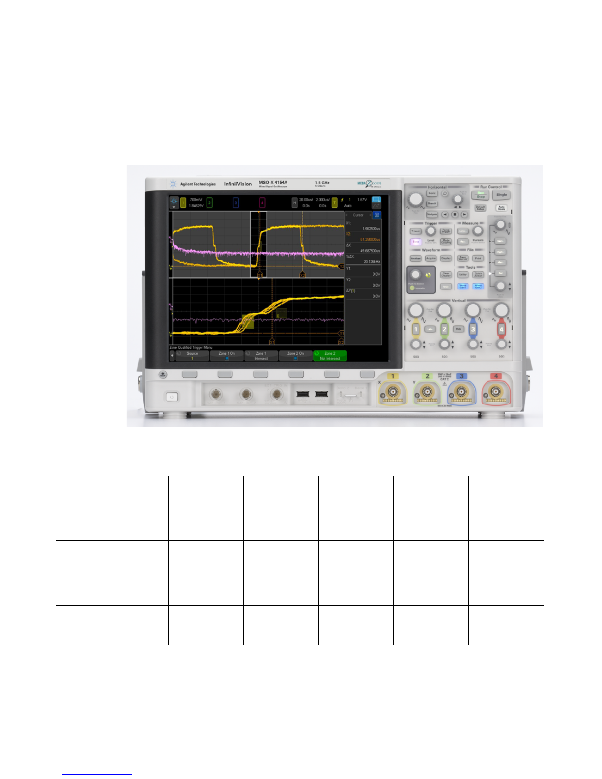
Zone Qualified Trigger 201

11 Trigger Mode/Coupling

To select the Auto or Normal trigger mode 206

To select the trigger coupling 208

To enable or disable trigger noise rejection 209

To enable or disable trigger HF Reject 209

To set the trigger holdoff 210

External Trigger Input 210

12 Acquisition Control

Running, Stopping, and Making Single Acquisitions (Run

Overview of Sampling 215

Maximum voltage at oscilloscope external trigger input 211

Control) 213

Sampling Theory 215 Aliasing 215 Oscilloscope Bandwidth and Sample Rate 216

Agilent InfiniiVision 4000 X-Series Oscilloscopes User's Guide 15

Oscilloscope Rise Time 217 Oscilloscope Bandwidth Required 218 Memory Depth and Sample Rate 219

Selecting the Acquisition Mode 219

Normal Acquisition Mode 220 Peak Detect Acquisition Mode 220 Averaging Acquisition Mode 223 High Resolution Acquisition Mode 225

Realtime Sampling Option 226

Realtime Sampling and Oscilloscope Bandwidth 227

Acquiring to Segmented Memory 228

Navigating Segments 229 Measurements, Statistics, and Infinite Persistence with

Segmented Memory 229 Segmented Memory Re-Arm Time 230 Saving Data from Segmented Memory 230

13 Cursors

To make cursor measurements 232

Cursor Examples 235

14 Measurements

To make automatic measurements 242

Measurements Summary 244

Snapshot All 246

Voltage Measurements 247

Peak-Peak 248 Maximum 248 Minimum 248 Amplitude 248 To p 249

16 Agilent InfiniiVision 4000 X-Series Oscilloscopes User's Guide

Base 250 Overshoot 250 Preshoot 251 Average 252 DC RMS 252 AC RMS 253 Ratio 255

Time Measurements 255

Period 256 Frequency 256 Counter 257 + Width 258 – Width 258 Burst Width 258 Duty Cycle 258 Rise Time 259 Fall Time 259 Delay 259 Phase 260 X at Min Y 262 X at Max Y 262

Agilent InfiniiVision 4000 X-Series Oscilloscopes User's Guide 17

Count Measurements 263

Positive Pulse Count 263 Negative Pulse Count 263 Rising Edge Count 264 Falling Edges Count 264

Mixed Measurements 264

Area 264

Measurement Thresholds 265

Measurement Window 267

Measurement Statistics 267

15 Mask Testing

To create a mask from a "golden" waveform (Automask) 271

Mask Test Setup Options 274

Mask Statistics 276

To manually modify a mask file 277

Building a Mask File 280

How is mask testing done? 282

16 Digital Voltmeter

17 Waveform Generator

To select generated waveform types and settings 287

To edit arbitrary waveforms 291

Creating New Arbitrary Waveforms 293 Editing Existing Arbitrary Waveforms 294 Capturing Other Waveforms to the Arbitrary Waveform 299

To output the waveform generator sync pulse 299

To specify the expected output load 300

To use waveform generator logic presets 300

To add noise to the waveform generator output 301

To add modulation to the waveform generator output 302

To set up Amplitude Modulation (AM) 303 To set up Frequency Modulation (FM) 304 To set up Frequency-Shift Keying Modulation (FSK) 306

To restore waveform generator defaults 307

To set up dual channel tracking 307

18 Agilent InfiniiVision 4000 X-Series Oscilloscopes User's Guide

18 Save/Recall (Setups, Screens, Data)

Saving Setups, Screen Images, or Data 309

To save setup files 311 To save BMP or PNG image files 311 To save CSV, ASCII XY, or BIN data files 312 Length Control 314 To save Lister data files 315 To save reference waveform files to a USB storage device 315 To save masks 316 To save arbitrary waveforms 316 To navigate storage locations 317 To en t e r file n a mes 317

Recalling Setups, Masks, or Data 318

To recall setup files 319 To recall mask files 319 To recall reference waveform files from a USB storage

device 319 To recall arbitrary waveforms 320

Recalling Default Setups 321

Performing a Secure Erase 321

19 Print (Screens)

To print the oscilloscope's display 323

To set up network printer connections 325

To specify the print options 326

To specify the palette option 327

20 Utility Settings

I/O Interface Settings 329

Setting up the Oscilloscope's LAN Connection 330

Agilent InfiniiVision 4000 X-Series Oscilloscopes User's Guide 19

To establish a LAN connection 331 Stand-alone (Point-to-Point) Connection to a PC 332

File Explorer 333

Setting Oscilloscope Preferences 335

To choose "expand about" center or ground 335 To disable/enable transparent backgrounds 336 To load the default label library 336 To set up the screen saver 336 To set AutoScale preferences 337

Setting the Oscilloscope's Clock 338

Setting the Rear Panel TRIG OUT Source 339

Setting the Reference Signal Mode 339

To supply a sample clock to the oscilloscope 340

Maximum input voltage at 10 MHz REF connector 340 To synchronize the timebase of two or more instruments 341

Performing Service Tasks 342

To perform user calibration 342 To perform hardware self test 344 To perform front panel self test 345 To display oscilloscope information 345 To display the user calibration status 345 To clean the oscilloscope 345 To check warranty and extended services status 346 To contact Agilent 346 To return the instrument 346

Configuring the [Quick Action] Key 347

21 Web Interface

Accessing the Web Interface 350

20 Agilent InfiniiVision 4000 X-Series Oscilloscopes User's Guide

22 Reference

Browser Web Control 351

Real Scope Remote Front Panel 352 Simple Remote Front Panel 353 Browser-Based Remote Front Panel 354 Remote Programming via the Web Interface 355 Remote Programming with Agilent IO Libraries 356

Save/Recall 357

Saving Files via the Web Interface 357 Recalling Files via the Web Interface 358

Get Image 359

Identification Function 360

Instrument Utilities 360

Setting a Password 363

Specifications and Characteristics 367

Measurement Category 367

Oscilloscope Measurement Category 368 Measurement Category Definitions 368 Transient Withstand Capability 369

Maximum input voltage at analog inputs 369

Maximum input voltage at digital channels 369

Environmental Conditions 369

Probes and Accessories 370

Passive Probes 371 Single-Ended Active Probes 371 Differential Probes 372 Current Probes 373

Agilent InfiniiVision 4000 X-Series Oscilloscopes User's Guide 21

Accessories Available 373

Loading Licenses and Displaying License Information 374

Licensed Options Available 375 Other Options Available 376 Upgrading to an MSO 376

Software and Firmware Updates 377

Binary Data (.bin) Format 377

Binary Data in MATLAB 378 Binary Header Format 378 Example Program for Reading Binary Data 381 Examples of Binary Files 381

CSV and ASCII XY files 384

CSV and ASCII XY file structure 385 Minimum and Maximum Values in CSV Files 385

Acknowledgements 386

23 CAN/LIN Triggering and Serial Decode

Setup for CAN Signals 387

CAN Triggering 389

CAN Serial Decode 391

Interpreting CAN Decode 392 CAN Totalizer 393 Interpreting CAN Lister Data 394 Searching for CAN Data in the Lister 395

Setup for LIN Signals 396

LIN Triggering 397

LIN Serial Decode 399

Interpreting LIN Decode 401 Interpreting LIN Lister Data 402

22 Agilent InfiniiVision 4000 X-Series Oscilloscopes User's Guide

Searching for LIN Data in the Lister 403

24 FlexRay Triggering and Serial Decode

Setup for FlexRay Signals 405

FlexRay Triggering 406

Triggering on FlexRay Frames 407 Triggering on FlexRay Errors 408 Triggering on FlexRay Events 408

FlexRay Serial Decode 409

Interpreting FlexRay Decode 410 FlexRay Totalizer 411 Interpreting FlexRay Lister Data 412 Searching for FlexRay Data in the Lister 413

25 I2C/SPI Triggering and Serial Decode

Setup for I2C Signals 415

I2C Triggering 416

I2C Serial Decode 420

Interpreting I2C Decode 421 Interpreting I2C Lister Data 423 Searching for I2C Data in the Lister 423

Setup for SPI Signals 424

SPI Triggering 428

SPI Serial Decode 430

Interpreting SPI Decode 432 Interpreting SPI Lister Data 433 Searching for SPI Data in the Lister 433

26 I2S Triggering and Serial Decode

Setup for I2S Signals 435

Agilent InfiniiVision 4000 X-Series Oscilloscopes User's Guide 23

I2S Triggering 438

I2S Serial Decode 441

Interpreting I2S Decode 442 Interpreting I2S Lister Data 443 Searching for I2S Data in the Lister 444

27 MIL-STD-1553/ARINC 429 Triggering and Serial Decode

Setup for MIL-STD-1553 Signals 445

MIL-STD-1553 Triggering 447

MIL-STD-1553 Serial Decode 448

Interpreting MIL-STD-1553 Decode 449 Interpreting MIL-STD-1553 Lister Data 450 Searching for MIL-STD-1553 Data in the Lister 451

Setup for ARINC 429 Signals 452

ARINC 429 Triggering 453

ARINC 429 Serial Decode 455

Interpreting ARINC 429 Decode 457 ARINC 429 Totalizer 458 Interpreting ARINC 429 Lister Data 459 Searching for ARINC 429 Data in the Lister 460

28 UART/RS232 Triggering and Serial Decode

Setup for UART/RS232 Signals 461

UART/RS232 Triggering 463

UART/RS232 Serial Decode 465

Interpreting UART/RS232 Decode 467 UART/RS232 Totalizer 468 Interpreting UART/RS232 Lister Data 469 Searching for UART/RS232 Data in the Lister 469

24 Agilent InfiniiVision 4000 X-Series Oscilloscopes User's Guide

29 USB 2.0 Triggering and Serial Decode

Setup for USB 2.0 Signals 471

USB 2.0 Triggering 473

USB 2.0 Serial Decode 475

Interpreting USB 2.0 Decode 476 Interpreting USB 2.0 Lister Data 478 Searching for USB 2.0 Data in the Lister 479

Index

Agilent InfiniiVision 4000 X-Series Oscilloscopes User's Guide 25

26 Agilent InfiniiVision 4000 X-Series Oscilloscopes User's Guide

Agilent InfiniiVision 4000 X-Series Oscilloscopes User's Guide

1 Getting Started

Inspect the Package Contents 27 Tilt the Oscilloscope for Easy Viewing 30 Power-On the Oscilloscope 30 Connect Probes to the Oscilloscope 31 Input a Waveform 32 Recall the Default Oscilloscope Setup 33 Use Auto Scale 33 Compensate Passive Probes 35 Learn the Front Panel Controls and Connectors 36 Learn the Touchscreen Controls 45 Learn the Rear Panel Connectors 56 Learn the Oscilloscope Display 58 Access the Built-In Quick Help 60

This chapter describes the steps you take when using the oscilloscope for the first time.

Inspect the Package Contents

• Inspect the shipping container for damage.

If your shipping container appears to be damaged, keep the shipping container or cushioning material until you have inspected the contents of the shipment for completeness and have checked the oscilloscope mechanically and electrically.

1 Getting Started

• Verify that you received the following items and any optional

accessories you may have ordered:

• InfiniiVision 4000 X- Series oscilloscope.

• Power cord (country of origin determines specific type).

• Oscilloscope probes:

• Two probes for 2-channel models.

• Four probes for 4- channel models.

• Digital probe kit (MSO models only).

• Documentation CD- ROM.

28 Agilent InfiniiVision 4000 X-Series Oscilloscopes User's Guide

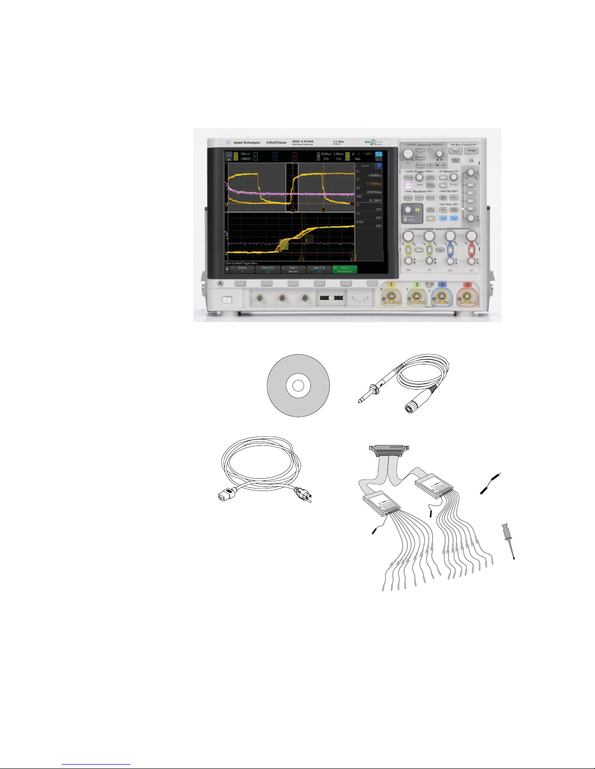
InfiniiVision 4000 X-Series oscilloscope

Getting Started 1

N2894A probes (Qty 2 or 4)

Documentation CD

Digital Probe Kit* (MSO models only)

Power cord (Based on country

f origin)

*N6450-60001 Digital Probe Kit contains: N6450-61601 16-channel cable (qyt 1) 01650-82103 2-inch probe ground leads (qyt 5) 5090-4832 Grabber (qyt 20)

Digital probe replacement parts are listed in the "Digital Channels" chapter.

See Also • “Accessories Available" on page 373

Agilent InfiniiVision 4000 X-Series Oscilloscopes User's Guide 29

1 Getting Started

Tilt the Oscilloscope for Easy Viewing

The oscilloscope can be tilted up for easier viewing. 1 Tilt the oscilloscope forward. Rotate the foot down and toward the rear

of the oscilloscope. The foot will lock into place.

2 Repeat for the other foot. 3 Rock the oscilloscope back so that it rests securely on its feet.

To retract the feet: 1 Tilt the oscilloscope forward. Press the foot release button and rotate

the foot up and toward the front of the oscilloscope.

2 Repeat for the other foot.

Power-On the Oscilloscope

Power

Requirements

Line voltage, frequency, and power:

• ~Line 100- 120 Vac, 50/60/400 Hz

• 100- 240 Vac, 50/60 Hz

• 120 W max

30 Agilent InfiniiVision 4000 X-Series Oscilloscopes User's Guide

Getting Started 1

WARNING

Ventilation

Requirements

To power -o n t he

oscilloscope

The air intake and exhaust areas must be free from obstructions. Unrestricted air flow is required for proper cooling. Always ensure that the air intake and exhaust areas are free from obstructions.

The fan draws air in from the left side and bottom of the oscilloscope and pushes it out behind the oscilloscope.

When using the oscilloscope in a bench- top setting, provide at least 2" clearance at the sides and 4" (100 mm) clearance above and behind the oscilloscope for proper cooling.

1 Connect the power cord to the rear of the oscilloscope, then to a

suitable AC voltage source. Route the power cord so the oscilloscope's feet and legs do not pinch the cord.

2 The oscilloscope automatically adjusts for input line voltages in the

range 100 to 240 VAC. The line cord provided is matched to the country of origin.

Always use a grounded power cord. Do not defeat the power cord ground.

3 Press the power switch.

The power switch is located on the lower left corner of the front panel. The oscilloscope will perform a self- test and will be operational in a few seconds.

Connect Probes to the Oscilloscope

1 Connect the oscilloscope probe to an oscilloscope channel BNC

connector.

2 Connect the probe's retractable hook tip to the point of interest on the

circuit or device under test. Be sure to connect the probe ground lead to a ground point on the circuit.

Agilent InfiniiVision 4000 X-Series Oscilloscopes User's Guide 31

1 Getting Started

CAUTION

WARNING

Maximum input voltage at analog inputs

CAT I 300 Vrms, 400 Vpk; transient overvoltage 1.6 kVpk

Ω input: 5 Vrms Input protection is enabled in 50 Ω mode and the 50 Ω load will

50 disconnect if greater than 5 Vrms is detected. However the inputs could still be damaged, depending on the time constant of the signal. The 50 functions when the oscilloscope is powered on.

With 10073C 10:1 probe: CAT I 500 Vpk, CAT II 400 Vpk With N2871A, N2872A, N2873A 10:1 probe: CAT I 400 Vpk, transient overvoltage

1.25 kVpk, CAT II 300 Vpk

Do not float the oscilloscope chassis

Defeating the ground connection and "floating" the oscilloscope chassis will probably result in inaccurate measurements and may also cause equipment damage. The probe ground lead is connected to the oscilloscope chassis and the ground wire in the power cord. If you need to measure between two live points, use a differential probe with sufficient dynamic range.

Ω input protection only

Do not negate the protective action of the ground connection to the oscilloscope. The oscilloscope must remain grounded through its power cord. Defeating the ground creates an electric shock hazard.

Input a Waveform

The first signal to input to the oscilloscope is the Demo 2, Probe Comp signal. This signal is used for compensating probes.

1 Connect an oscilloscope probe from channel 1 to the Demo 2 (Probe

Comp) terminal on the front panel.

2 Connect the probe's ground lead to the ground terminal (next to the

Demo 2 terminal).

32 Agilent InfiniiVision 4000 X-Series Oscilloscopes User's Guide

Recall the Default Oscilloscope Setup

To recall the default oscilloscope setup: 1 Press [Default Setup].

The default setup restores the oscilloscope's default settings. This places the oscilloscope in a known operating condition. The major default settings are:

Table 2 Default Configuration Settings

Horizontal Normal mode, 100 µs/div scale, 0 s delay, center time reference.

Getting Started 1

Use Auto Scale

Vertical (Analog)

Trigger Edge trigger, Auto trigger mode, 0 V level, channel 1 source, DC coupling,

Display Persistence off, 20% grid intensity, 50% waveform intensity.

Other Acquire mode normal, [Run/Stop] to Run, cursors and measurements off.

Labels All custom labels that you have created in the Label Library are preserved (not

In the Save/Recall Menu, there are also options for restoring the complete factory settings (see “Recalling Default Setups" on page 321) or performing a secure erase (see “Performing a Secure Erase" on page 321).

Use [Auto Scale] to automatically configure the oscilloscope to best display the input signals.

1 Press [Auto Scale].

Channel 1 on, 5 V/div scale, DC coupling, 0 V position, 1 M

rising edge slope, 40 ns holdoff time.

erased), but all channel labels will be set to their original names.

Ω impedance.

You should see a waveform on the oscilloscope's display similar to this:

Agilent InfiniiVision 4000 X-Series Oscilloscopes User's Guide 33

1 Getting Started

How AutoScale

Works

2 If you want to return to the oscilloscope settings that existed before,

press Undo AutoScale.

3 If you want to enable "fast debug" autoscaling, change the channels

autoscaled, or preserve the acquisition mode during autoscale, press Fast Debug, Channels, or Acq Mode.

These are the same softkeys that appear in the AutoScale Preferences Menu. See “To set AutoScale preferences" on page 337.

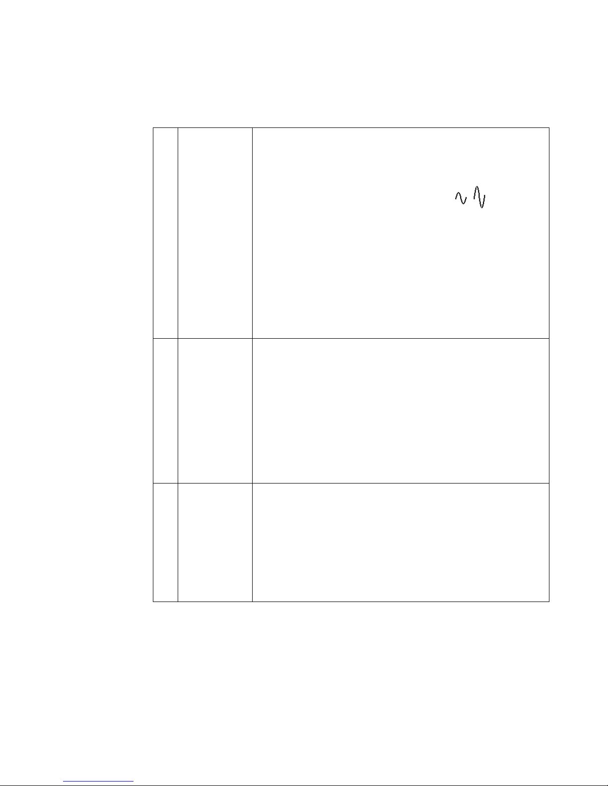
If you see the waveform, but the square wave is not shaped correctly as shown above, perform the procedure “Compensate Passive Probes" on page 35.

If you do not see the waveform, make sure the probe is connected securely to the front panel channel input BNC and to the left side, Demo 2, Probe Comp terminal.

Auto Scale analyzes any waveforms present at each channel and at the external trigger input. This includes the digital channels, if connected.

34 Agilent InfiniiVision 4000 X-Series Oscilloscopes User's Guide

Auto Scale finds, turns on, and scales any channel with a repetitive waveform that has a frequency of at least 25 Hz, a duty cycle greater than

0.5%, and an amplitude of at least 10 mV peak- to- peak. Any channels where no signal is found are turned off.

The trigger source is selected by looking for the first valid waveform starting with external trigger, then continuing with the lowest number analog channel up to the highest number analog channel, and finally (if digital probes are connected) the highest number digital channel.

During Auto Scale, the delay is set to 0.0 seconds, the horizontal time/div (sweep speed) setting is a function of the input signal (about 2 periods of the triggered signal on the screen), and the triggering mode is set to Edge.

Compensate Passive Probes

Each oscilloscope passive probe must be compensated to match the input characteristics of the oscilloscope channel to which it is connected. A poorly compensated probe can introduce significant measurement errors.

1 Input the Probe Comp signal (see “Input a Waveform" on page 32).

Getting Started 1

2 Press [Default Setup] to recall the default oscilloscope setup (see “Recall

the Default Oscilloscope Setup" on page 33).

3 Press [Auto Scale] to automatically configure the oscilloscope for the

Probe Comp signal (see “Use Auto Scale" on page 33).

4 Press the channel key to which the probe is connected ([1], [2], etc.). 5 In the Channel Menu, press Probe. 6 In the Channel Probe Menu, press Probe Check; then, follow the

instructions on- screen.

If necessary, use a nonmetallic tool (supplied with the probe) to adjust the trimmer capacitor on the probe for the flattest pulse possible.

On the N2862/63/90 probes, the trimmer capacitor is the yellow adjustment on the probe tip. On other probes, the trimmer capacitor is located on the probe BNC connector.

Agilent InfiniiVision 4000 X-Series Oscilloscopes User's Guide 35

1 Getting Started

Perfectly compensated

Over compensated

Under compensated

7 Connect probes to all other oscilloscope channels (channel 2 of a

2- channel oscilloscope, or channels 2, 3, and 4 of a 4- channel oscilloscope).

8 Repeat the procedure for each channel.

Learn the Front Panel Controls and Connectors

On the front panel, key refers to any key (button) you can press.

Softkey specifically refers to the six keys that are directly below the

display. The legend for these keys is directly above them, on the display. Their functions change as you navigate through the oscilloscope's menus.

For the following figure, refer to the numbered descriptions in the table that follows.

36 Agilent InfiniiVision 4000 X-Series Oscilloscopes User's Guide

Getting Started 1

14. Tools keys

1. Power switch

2. Softkeys

3. [Intensity] key

4. Entry knob

6. Trigger controls

5. Waveform keys

18. Demo 2, Ground, and Demo 1

terminals

17. Analog channel

inputs

19. USB Host

ports

15. [Help] key

13. File keys

8. Run Control keys

12. Measure controls

11. Additional waveform controls

7. Horizontal controls

10. [Auto Scale] key

9. [Default Setup] key

16. Vertical controls

21. Waveform generator

outputs

20. EXT TRIG IN connector

Back

1. Power switch Press once to switch power on; press again to switch power off. See

“Power-On the Oscilloscope" on page 30.

2. Softkeys The functions of these keys change based upon the menus shown on the display directly above the keys.

The Back/Up key moves up in the softkey menu hierarchy. At the

top of the hierarchy, the Back/Up key turns the menus off, and oscilloscope information is shown instead.

3. [Intensity] key Press the key to illuminate it. When illuminated, turn the Entry knob to adjust waveform intensity. You can vary the intensity control to bring out signal detail, much like an analog oscilloscope. Digital channel waveform intensity is not adjustable. More details about using the Intensity control to view signal detail are on

“To adjust waveform intensity" on page 149.

Agilent InfiniiVision 4000 X-Series Oscilloscopes User's Guide 37

1 Getting Started

4. Entry knob The Entry knob is used to select items from menus and to change values. The function of the Entry knob changes based upon the current menu and softkey selections.

Note that the curved arrow symbol above the entry knob illuminates whenever the entry knob can be used to select a value. Also,

note that when the Entry knob symbol appears on a softkey, you can use the Entry knob, to select values. Often, rotating the Entry knob is enough to make a selection. Sometimes, you can push the Entry knob to enable or disable a selection. Pushing the Entry knob also makes popup menus disappear.

5. Waveform keys [Analyze] key — Press this key to access analysis features like:

• Trigger level setting.

• Measurement threshold setting.

• Video trigger automatic set up and display.

• Mask testing (see Chapter 15, “Mask Testing,” starting on page 271).

• The DSOX4PWR power measurement and analysis application.

• Digital voltmeter (DVM) (see Chapter 16, “Digital Voltmeter,” starting

on page 283). The [Acquire] key lets you select Normal, Peak Detect, Averaging, or High Resolution acquisition modes (see “Selecting the Acquisition

Mode" on page 219) and use segmented memory (see “Acquiring to Segmented Memory" on page 228).

The [Display] key lets you access the menu where you can enable persistence (see “To set or clear persistence" on page 151), clear the display, and adjust the display grid (graticule) intensity (see “To adjust

the grid intensity" on page 153).

[Touch] key — Press this key to disable/enable the touchscreen.

6. Trigger controls These controls determine how the oscilloscope triggers to capture data.

38 Agilent InfiniiVision 4000 X-Series Oscilloscopes User's Guide

See Chapter 10, “Triggers,” starting on page 165 and Chapter 11, “Trigger Mode/Coupling,” starting on page 205.

Getting Started 1

7. Horizontal controls

The Horizontal controls consist of:

• Horizontal scale knob — Turn the knob in the Horizontal section that

is marked to adjust the time/div (sweep speed) setting. The symbols under the knob indicate that this control has the effect of spreading out or zooming in on the waveform using the horizontal scale.

• Horizontal position knob — Turn the knob marked to pan through the waveform data horizontally. You can see the captured waveform before the trigger (turn the knob clockwise) or after the trigger (turn the knob counterclockwise). If you pan through the waveform when the oscilloscope is stopped (not in Run mode) then you are looking at the waveform data from the last acquisition taken.

• [Horiz] key — Press this key to open the Horizontal Menu where you can select XY and Roll modes, enable or disable Zoom, enable or disable horizontal time/division fine adjustment, and select the trigger time reference point.

• Zoom key — Press the zoom key to split the oscilloscope display into Normal and Zoom sections without opening the Horizontal Menu.

•[Search] key — Lets you search for events in the acquired data.

•[Navigate] keys — Press these keys to navigate through captured

data via time, search events, or segmented memory acquisition. See

“Navigating the Time Base" on page 75.

For more information see Chapter 2, “Horizontal Controls,” starting on page 63.

8. Run Control keys

9. [Default Setup] key

When the [Run/Stop] key is green, the oscilloscope is running, that is, acquiring data when trigger conditions are met. To stop acquiring data, press [Run/Stop]. When the [Run/Stop] key is red, data acquisition is stopped. To start acquiring data, press [Run/Stop]. To capture and display a single acquisition (whether the oscilloscope is running or stopped), press [Single]. The [Single] key is yellow until the oscilloscope triggers. For more information, see “Running, Stopping, and Making Single

Acquisitions (Run Control)" on page 213.

Press this key to restore the oscilloscope's default settings (details on

“Recall the Default Oscilloscope Setup" on page 33).

Agilent InfiniiVision 4000 X-Series Oscilloscopes User's Guide 39

1 Getting Started

10. [Auto Scale] key

11. Additional waveform controls

When you press the [AutoScale] key, the oscilloscope will quickly determine which channels have activity, and it will turn these channels on and scale them to display the input signals. See “Use Auto Scale" on page 33.

The additional waveform controls consist of:

•[Math] key — provides access to math (add, subtract, etc.) waveform functions. See Chapter 4, “Math Waveforms,” starting on page 89.

•[Ref] key — provides access to reference waveform functions. Reference waveforms are saved waveforms that can be displayed and compared against other analog channel or math waveforms. Also, measurements can be made on reference waveforms. See Chapter 5, “Reference Waveforms,” starting on page 119.

•[Digital] key — Press this key to turn the digital channels on or off (the arrow to the left will illuminate). When the arrow to the left of the [Digital] key is illuminated, the upper multiplexed knob selects (and highlights in red) individual digital channels, and the lower multiplexed knob positions the selected digital channel. If a trace is repositioned over an existing trace the indicator at the left edge of the trace will change from Dnn designation (where nn is a one or two digit channel number from 0 to 15) to D*. The "*" indicates that two or more channels are overlaid. You can rotate the upper knob to select an overlaid channel, then rotate the lower knob to position it just as you would any other channel. For more information on digital channels see Chapter 6, “Digital Channels,” starting on page 123.

•[Serial] key — This key is used to enable serial decode. The multiplexed scale and position knobs are not used with serial decode. For more information on serial decode, see Chapter 7, “Serial Decode,” starting on page 143.

• Multiplexed scale knob — This scale knob is used with Math, Ref, or Digital waveforms, whichever has the illuminated arrow to the left. For math and reference waveforms, the scale knob acts like an analog channel vertical scale knob.

• Multiplexed position knob — This position knob is used with Math, Ref, or Digital waveforms, whichever has the illuminated arrow to the left. For math and reference waveforms, the position knob acts like an analog channel vertical position knob.

40 Agilent InfiniiVision 4000 X-Series Oscilloscopes User's Guide

Getting Started 1

12. Measure controls

13. File keys Press the [Save/Recall] key to save or recall a waveform or setup. See

14. Tools keys The Tools keys consist of:

The measure controls consist of:

• Cursors knob — Push this knob to select cursors from a popup menu. Then, after the popup menu closes (either by timeout or by pushing the knob again), rotate the knob to adjust the selected cursor position.

• [Cursors] key — Press this key to open a menu that lets you select the cursors mode and source.

•[Meas] key — Press this key to access a set of predefined measurements. See Chapter 14, “Measurements,” starting on page

241.

Chapter 18, “Save/Recall (Setups, Screens, Data),” starting on page 309.

The [Print] key opens the Print Configuration Menu so you can print the displayed waveforms. See Chapter 19, “Print (Screens),” starting on page

323.

• [Utility] key — Press this key to access the Utility Menu, which lets you configure the oscilloscope's I/O settings, use the file explorer, set preferences, access the service menu, and choose other options. See

Chapter 20, “Utility Settings,” starting on page 329.

• [Quick Action] key — Press this key to perform the selected quick action: measure all snapshot, print, save, recall, freeze display, and more. See “Configuring the [Quick Action] Key" on page 347.

• [Wave Gen1], [Wave Gen2] keys — Press these keys to access waveform generator functions. See Chapter 17, “Waveform Generator,” starting on page 287.

15. [Help] key Opens the Help Menu where you can display overview help topics and select the Language. See also “Access the Built-In Quick Help" on page 60.

Agilent InfiniiVision 4000 X-Series Oscilloscopes User's Guide 41

1 Getting Started

16. Vertical

controls

17. Analog channel

inputs

The Vertical controls consist of:

• Analog channel on/off keys — Use these keys to switch a channel on

or off, or to access a channel's menu in the softkeys. There is one channel on/off key for each analog channel.

• Vertical scale knob — There are knobs marked for each

channel. Use these knobs to change the vertical sensitivity (gain) of each analog channel.

• Vertical position knobs — Use these knobs to change a channel's

vertical position on the display. There is one Vertical Position control for each analog channel.

•[Label] key — Press this key to access the Label Menu, which lets

you enter labels to identify each trace on the oscilloscope display. See

Chapter 9, “Labels,” starting on page 157.

For more information, see Chapter 3, “Vertical Controls,” starting on page 79.

Attach oscilloscope probes or BNC cables to these BNC connectors. With the InfiniiVision 4000 X-Series oscilloscopes, you can set the input impedance of the analog channels to either 50

specify channel input impedance" on page 83.

The InfiniiVision 4000 X-Series oscilloscopes also provide the AutoProbe interface. The AutoProbe interface uses a series of contacts directly below the channel's BNC connector to transfer information between the oscilloscope and the probe. When you connect a compatible probe to the oscilloscope, the AutoProbe interface determines the type of probe and sets the oscilloscope's parameters (units, offset, attenuation, coupling, and impedance) accordingly.

Ω or 1 MΩ. See “To

18. Demo 2, Ground, and Demo 1 terminals

42 Agilent InfiniiVision 4000 X-Series Oscilloscopes User's Guide

• Demo 2 terminal — This terminal outputs the Probe Comp signal which helps you match a probe's input capacitance to the oscilloscope channel to which it is connected. See “Compensate

Passive Probes" on page 35. With certain licensed features, the

oscilloscope can also output demo or training signals on this terminal.

• Ground terminal — Use the ground terminal for oscilloscope probes connected to the Demo 1 or Demo 2 terminals.

• Demo 1 terminal — With certain licensed features, the oscilloscope can output demo or training signals on this terminal.

Getting Started 1

19. USB Host ports These ports are for connecting a USB mass storage device, printer, mouse, or keyboard to the oscilloscope. Connect a USB compliant mass storage device (flash drive, disk drive, etc.) to save or recall oscilloscope setup files and reference waveforms or to save data and screen images. See Chapter 18, “Save/Recall (Setups, Screens, Data),” starting on page 309. To print, connect a USB compliant printer. For more information about printing see Chapter 19, “Print (Screens),” starting on page 323. You can also use the USB port to update the oscilloscope's system software when updates are available. You do not need to take special precautions before removing the USB mass storage device from the oscilloscope (you do not need to "eject" it). Simply unplug the USB mass storage device from the oscilloscope when the file operation is complete.

CAUTION: Do not connect a host computer to the oscilloscope's USB host port. Use the device port. A host computer sees the

oscilloscope as a device, so connect the host computer to the oscilloscope's device port (on the rear panel). See “I/O Interface

Settings" on page 329.

There is a third USB host port on the back panel.

20. EXT TRIG IN

connector

21. Waveform

generator outputs

External trigger input BNC connector. See “External Trigger Input" on page 210 for an explanation of this feature.

Built-in, license-enabled 2-channel waveform generator can output arbitrary, sine, square, ramp, pulse, DC, noise, sine cardinal, exponential rise, exponential fall, cardiac, or Gaussian pulse waveforms on the Gen Out 1 or Gen Out 2 BNC connectors. Modulated waveforms are available on WaveGen1 except for arbitrary, pulse, DC, and noise waveforms. Press the [Wave Gen1] or [Wave Gen2] keys to set up the waveform generator. See Chapter 17, “Waveform Generator,” starting on page 287.

Front Panel Overlays for Different Languages

Front panel overlays, which have translations for the English front panel keys and label text, are available in 10 languages. The appropriate overlay is included when the localization option is chosen at time of purchase.

To install a front panel overlay:

1 Gently pull on the front panel knobs to remove them. 2 Insert the overlay's side tabs into the slots on the front panel.

Agilent InfiniiVision 4000 X-Series Oscilloscopes User's Guide 43

1 Getting Started

3 Reinstall the front panel knobs.

Front panel overlays may be ordered from "www.parts.agilent.com" using the following part numbers:

Language 2 Channel Overlay 4 Channel Overlay

French 54709-94315 54709-94316

German 54709-94313 54709-94314

Italian 54709-94317 54709-94318

Japanese 54709-94321 54709-94322

Korean 54709-94311 54709-94312

Portuguese 54709-94323 54709-94324

Russian 54709-94325 54709-94326

Simplified Chinese 54709-94306 54709-94308

Spanish 54709-94319 54709-94320

Traditional Chinese 54709-94309 54709-94310

44 Agilent InfiniiVision 4000 X-Series Oscilloscopes User's Guide

Learn the Touchscreen Controls

When the [Touch] key is lit, you can control the oscilloscope by touching different areas of the screen. You can:

• “Draw Rectangles for Waveform Zoom or Zone Trigger Set Up" on

page 45

• “Drag Waveforms Left and Right to Change the Horizontal Position" on

page 46

• “Select Sidebar Information or Controls" on page 47

• “Undock Sidebar Dialogs by Dragging" on page 48

• “Select Dialog Menus and Close Dialogs" on page 49

• “Drag Cursors" on page 49

• “Touch Softkeys and Menus On the Screen" on page 49

• “Enter Names Using Alpha-Numeric Keypad Dialogs" on page 50

• “Change Waveform Offsets By Dragging Ground Reference Icons" on

page 51

Getting Started 1

• “Access Controls and Menus Via the Spark Icon" on page 52

• “Turn Channels On/Off and Open Scale/Offset Dialogs" on page 54

• “Access the Horizontal Menu and Open the Scale/Delay Dialog" on

page 54

• “Access the Trigger Menu, Change the Trigger Mode, and Open the

Trigger Level Dialog" on page 55

• “Use a USB Mouse and/or Keyboard for Touchscreen Controls" on

page 56

Draw Rectangles for Waveform Zoom or Zone Trigger Set Up

1 Touch the upper-right corner to select the rectangle draw mode.

Agilent InfiniiVision 4000 X-Series Oscilloscopes User's Guide 45

1 Getting Started

2 Drag your finger across the screen to draw a rectangle. 3 Take your finger off the screen. 4 Touch the desired option from the popup menu.

Drag Waveforms Left and Right to Change the Horizontal Position

1 Touch the upper-right corner to select the horizontal drag mode.

46 Agilent InfiniiVision 4000 X-Series Oscilloscopes User's Guide

Getting Started 1

2 Drag your finger across the screen to change the horizontal delay.

Select Sidebar Information or Controls

1 Touch the blue menu icon in the sidebar. 2 In the popup menu, touch the type of information or controls you want

to see in the sidebar.

Agilent InfiniiVision 4000 X-Series Oscilloscopes User's Guide 47

1 Getting Started

Undock Sidebar Dialogs by Dragging

Sidebar dialogs can be undocked and placed anywhere on the screen. 1 Drag the sidebar dialog title wherever you like.

This lets you view multiple types of information or controls at the same time.

48 Agilent InfiniiVision 4000 X-Series Oscilloscopes User's Guide

Select Dialog Menus and Close Dialogs

• Touch the blue menu icon in the dialog for options.

• Touch the red "X" icon to close a dialog.

Drag Cursors

When cursors are displayed, you can drag the name handles to position them.

Getting Started 1

Touch Softkeys and Menus On the Screen

• Touch onscreen softkey labels to select them.

Agilent InfiniiVision 4000 X-Series Oscilloscopes User's Guide 49

1 Getting Started

This is the same as pressing the softkey keys.

• When softkeys provide menus, double-touch to select a menu item.

This may be an easier than selecting a menu item via the Entry knob.

Enter Names Using Alpha-Numeric Keypad Dialogs

Some softkeys open alpha- numeric dialogs that let you touch to enter names.

50 Agilent InfiniiVision 4000 X-Series Oscilloscopes User's Guide

Getting Started 1

Change Waveform Offsets By Dragging Ground Reference Icons

You can drag ground icons to change a waveform's vertical offset.

Agilent InfiniiVision 4000 X-Series Oscilloscopes User's Guide 51

1 Getting Started

Access Controls and Menus Via the Spark Icon

1 Touch the upper-left spark icon to open the main menu.

2 Touch left side controls to perform oscilloscope operations.

52 Agilent InfiniiVision 4000 X-Series Oscilloscopes User's Guide

Getting Started 1

3 Touch menu items and submenu items to access menus and additional

controls.

Agilent InfiniiVision 4000 X-Series Oscilloscopes User's Guide 53

1 Getting Started

Turn Channels On/Off and Open Scale/Offset Dialogs

• Touch channel numbers to turn them on or off.

• When channels are on, touch the scale and offset values to access a

dialog for changing them.

Access the Horizontal Menu and Open the Scale/Delay Dialog

• Touch "H" to access the Horizontal Menu.

• Touch the horizontal scale and delay values to access a dialog for

changing them.

54 Agilent InfiniiVision 4000 X-Series Oscilloscopes User's Guide

Getting Started 1

Access the Trigger Menu, Change the Trigger Mode, and Open the Trigger Level Dialog

• Touch "T" to access the Trigger Menu.

• Touch the trigger level value(s) to access a dialog for changing the

level(s).

• Touch "Auto" or "Trig'd" to quickly toggle the trigger mode.

Agilent InfiniiVision 4000 X-Series Oscilloscopes User's Guide 55

1 Getting Started

Use a USB Mouse and/or Keyboard for Touchscreen Controls

Connecting a USB mouse gives you a mouse pointer on the display. Mouse clicks and drags behave the same as screen touches and finger drags.

If you connect a USB keyboard, you can use it to enter values in alpha- numeric keypad dialogs.

Learn the Rear Panel Connectors

For the following figure, refer to the numbered descriptions in the table that follows.

56 Agilent InfiniiVision 4000 X-Series Oscilloscopes User's Guide

Getting Started 1

9. USB Device port

8. USB Host port

1. Power cord connector

2. Kensington lock hole

3. TRIG OUT connector

5. Calibration protect switch

4. 10 MHz REF connector

6. Digital channel inputs

7. VGA Video Out

10. LAN port

1. Power cord

connector

2. Kensington

lock hole

3. TRIG OUT

connector

4. 10 MHz REF

connector

5. Calibration

protect switch

Attach the power cord here.

This is where you can attach a Kensington lock for securing the instrument.

Trigger output BNC connector. See “Setting the Rear Panel TRIG OUT

Source" on page 339.

For synchronizing the timebase of multiple instruments. See “Setting the

Reference Signal Mode" on page 339.

See “To perform user calibration" on page 342.

Agilent InfiniiVision 4000 X-Series Oscilloscopes User's Guide 57

1 Getting Started

6. Digital channel

inputs

7. VGA video

output

8. USB Host port This port functions identically to the USB host port on the front panel.

9. USB Device

port

10. LAN port Lets you print to network printers (see Chapter 19, “Print (Screens),”

Connect the digital probe cable to this connector (MSO models only). See

Chapter 6, “Digital Channels,” starting on page 123.

Lets you connect an external monitor or projector to provide a larger display or to provide a display at a viewing position away from the oscilloscope. The oscilloscope's built-in display remains on even when an external display is connected. The video output connector is always active. For optimal video quality and performance, we recommend you use a shielded video cable with ferrite cores.

USB Host Port is used for saving data from the oscilloscope and loading software updates. See also USB Host port (see page 43).

This port is for connecting the oscilloscope to a host PC. You can issue remote commands from a host PC to the oscilloscope via the USB device port. See “Remote Programming with Agilent IO Libraries" on page 356.

starting on page 323) and access the oscilloscope's built-in web server. See Chapter 21, “Web Interface,” starting on page 349 and “Accessing

the Web Interface" on page 350.

Learn the Oscilloscope Display

The oscilloscope display contains acquired waveforms, setup information, measurement results, and the softkey definitions.

58 Agilent InfiniiVision 4000 X-Series Oscilloscopes User's Guide

Getting Started 1

Analog channel sensitivity

Status line

Analog channels and ground levels

Trigger level

Digital channels

Softkeys

Menu line

Trigger point, time reference

Delay time

Time/ div

Run/Stop status

Trigger type

Trigger source

Measurements

Trigger level or digital threshold

Sidebar information and controls area

Cursors defining measurement

Measurement statistics

Figure 1 Interpreting the oscilloscope display

Status line The top line of the display contains vertical, horizontal, and trigger setup

Display area The display area contains the waveform acquisitions, channel identifiers, and

information.

analog trigger, and ground level indicators. Each analog channel's information appears in a different color. Signal detail is displayed using 256 levels of intensity. For more information about viewing signal detail see “To adjust waveform intensity" on page 149. For more information about display modes see Chapter 8, “Display Settings,” starting on page 149.

Agilent InfiniiVision 4000 X-Series Oscilloscopes User's Guide 59

1 Getting Started

Back

Sidebar information and controls area

Menu line This line normally contains menu name or other information associated with

Softkey labels These labels describe softkey functions. Typically, softkeys let you set up

The sidebar information area can contain summary, cursors, measurements, or digital voltmeter information dialogs or it can contain navigation and other control dialogs. For more information, see:

• “Select Sidebar Information or Controls" on page 47

• “Undock Sidebar Dialogs by Dragging" on page 48

the selected menu.

additional parameters for the selected mode or menu.

Pressing the Back/Up key at the top of the menu hierarchy turns off softkey labels and displays additional status information describing channel offset and other configuration parameters.

Access the Built-In Quick Help

To view Q ui ck

Help

1 Press and hold the key or softkey for which you would like to view

help.

60 Agilent InfiniiVision 4000 X-Series Oscilloscopes User's Guide

Getting Started 1

Quick Help message

Press and hold front panel key or softkey (or right-click softkey when using web browser remote front panel).

To s elect th e us er

interface and

Quick Help

language

Quick Help remains on the screen until another key is pressed or a knob is turned.

To select the user interface and Quick Help language:

1 Press [Help], then press the Language softkey. 2 Repeatedly press and release the Language softkey or rotate the Entry

knob until the desired language is selected.

The following languages are available: English, French, German, Italian, Japanese, Korean, Portuguese, Russian, Simplified Chinese, Spanish, and Traditional Chinese.

Agilent InfiniiVision 4000 X-Series Oscilloscopes User's Guide 61

1 Getting Started

62 Agilent InfiniiVision 4000 X-Series Oscilloscopes User's Guide

Agilent InfiniiVision 4000 X-Series Oscilloscopes User's Guide

2 Horizontal Controls

To adjust the horizontal (time/div) scale 65 To adjust the horizontal delay (position) 65 Panning and Zooming Single or Stopped Acquisitions 66 To change the horizontal time mode (Normal, XY, or Roll) 67 To display the zoomed time base 71 To change the horizontal scale knob's coarse/fine adjustment setting 73 To position the time reference (left, center, right) 73 Searching for Events 74 Navigating the Time Base 75

The horizontal controls include:

• The horizontal scale and position knobs.

• The [Horiz] key for accessing the Horizontal Menu.

• The zoom key for quickly enabling/disabling the split- screen zoom

display.

• The [Search] key for finding events on analog channels or in serial

decode.

• The [Navigate] keys for navigating time, search events, or segmented

memory acquisitions.

• Touchscreen controls for setting the horizontal scale and position

(delay), accessing the Horizontal Menu, and navigating.

The following figure shows the Horizontal Menu which appears after pressing the [Horiz] key.

2 Horizontal Controls

Trigger point

Sample rate

Time reference

Delay time

Time/ div

Trigger source

Trigger level or threshold

XY or Roll mode

Normal time mode

Zoomed time base

Fine control

Time reference

Figure 2 Horizontal Menu

The Horizontal Menu lets you select the time mode (Normal, XY, or Roll), enable Zoom, set the time base fine control (vernier), and specify the time reference.

The current sample rate is displayed in the right- side information area.

64 Agilent InfiniiVision 4000 X-Series Oscilloscopes User's Guide

To adjust the horizontal (time/div) scale

1 Turn the large horizontal scale (sweep speed) knob marked to

change the horizontal time/div setting.

You can also make this adjustment using the touchscreen. See "Access

the Horizontal Menu and Open the Scale/Delay Dialog" on page 54.

Notice how the time/div information in the status line changes. The ∇ symbol at the top of the display indicates the time reference point.

The horizontal scale knob works (in the Normal time mode) while acquisitions are running or when they are stopped. When running, adjusting the horizontal scale knob changes the sample rate. When stopped, adjusting the horizontal scale knob lets you zoom into acquired data. See "Panning and Zooming Single or Stopped Acquisitions" on page 66.

Horizontal Controls 2

Note that the horizontal scale knob has a different purpose in the Zoom display. See "To display the zoomed time base" on page 71.

To adjust the horizontal delay (position)

1 Turn the horizontal delay (position) knob ( ).

The trigger point moves horizontally, pausing at 0.00 s (mimicking a mechanical detent), and the delay value is displayed in the status line.

You can also make this adjustment using the touchscreen. See "Drag

Waveforms Left and Right to Change the Horizontal Position" on

page 46 and "Access the Horizontal Menu and Open the Scale/Delay

Dialog" on page 54.

Changing the delay time moves the trigger point (solid inverted triangle) horizontally and indicates how far it is from the time reference point (hollow inverted triangle ∇). These reference points are indicated along the top of the display grid.

Agilent InfiniiVision 4000 X-Series Oscilloscopes User's Guide 65

2 Horizontal Controls

Figure 2 shows the trigger point with the delay time set to 200 µs. The

delay time number tells you how far the time reference point is located from the trigger point. When delay time is set to zero, the delay time indicator overlays the time reference indicator.

All events displayed left of the trigger point happened before the trigger occurred. These events are called pre- trigger information, and they show events that led up to the trigger point.

Everything to the right of the trigger point is called post- trigger information. The amount of delay range (pre- trigger and post- trigger information) available depends on the time/div selected and memory depth.

The horizontal position knob works (in the Normal time mode) while acquisitions are running or when they are stopped. When running, adjusting the horizontal scale knob changes the sample rate. When stopped, adjusting the horizontal scale knob lets you zoom into acquired data. See "Panning and Zooming Single or Stopped Acquisitions" on page 66.

Note that the horizontal position knob has a different purpose in the Zoom display. See "To display the zoomed time base" on page 71.

Panning and Zooming Single or Stopped Acquisitions

When the oscilloscope is stopped, use the horizontal scale and position knobs to pan and zoom your waveform. The stopped display may contain several acquisitions worth of information, but only the last acquisition is available for pan and zoom.

The ability to pan (move horizontally) and scale (expand or compress horizontally) an acquired waveform is important because of the additional insight it can reveal about the captured waveform. This additional insight is often gained from seeing the waveform at different levels of abstraction. You may want to view both the big picture and the specific little picture details.

The ability to examine waveform detail after the waveform has been acquired is a benefit generally associated with digital oscilloscopes. Often this is simply the ability to freeze the display for the purpose of measuring with cursors or printing the screen. Some digital oscilloscopes

66 Agilent InfiniiVision 4000 X-Series Oscilloscopes User's Guide

go one step further by including the ability to further examine the signal

NOTE

details after acquiring them by panning through the waveform and changing the horizontal scale.

There is no limit imposed on the scaling ratio between the time/div used to acquire the data and the time/div used to view the data. There is, however, a useful limit. This useful limit is somewhat a function of the signal you are analyzing.

Zooming into stopped acquisitions

The screen will still contain a relatively good display if you zoom-in horizontally by a factor of 1000 and zoom-in vertically by a factor of 10 to display the information from where it was acquired. Remember that you can only make automatic measurements on displayed data.

To change the horizontal time mode (Normal, XY, or Roll)

Horizontal Controls 2

1 Press [Horiz]. 2 In the Horizontal Menu, press Time Mode; then, select:

• Normal — the normal viewing mode for the oscilloscope.

In the Normal time mode, signal events occurring before the trigger are plotted to the left of the trigger point (▼) and signal events after the trigger plotted to the right of the trigger point.

• XY — XY mode changes the display from a volts-versus- time display

to a volts-versus-volts display. The time base is turned off. Channel 1 amplitude is plotted on the X- axis and Channel 2 amplitude is plotted on the Y- axis.

You can use XY mode to compare frequency and phase relationships between two signals. XY mode can also be used with transducers to display strain versus displacement, flow versus pressure, volts versus current, or voltage versus frequency.

Use the cursors to make measurements on XY mode waveforms.

For more information about using XY mode for measurements, refer to "XY Time Mode" on page 68.

Agilent InfiniiVision 4000 X-Series Oscilloscopes User's Guide 67

2 Horizontal Controls

• Roll — causes the waveform to move slowly across the screen from

right to left. It only operates on time base settings of 50 ms/div and slower. If the current time base setting is faster than the 50 ms/div limit, it will be set to 50 ms/div when Roll mode is entered.

In Roll mode there is no trigger. The fixed reference point on the screen is the right edge of the screen and refers to the current moment in time. Events that have occurred are scrolled to the left of the reference point. Since there is no trigger, no pre- trigger information is available.

If you would like to pause the display in Roll mode press the [Single] key. To clear the display and restart an acquisition in Roll mode, press the [Single] key again.

Use Roll mode on low-frequency waveforms to yield a display much like a strip chart recorder. It allows the waveform to roll across the display.

XY Time Mode

Example This exercise shows a common use of the XY display mode by measuring

The XY time mode converts the oscilloscope from a volts- versus- time display to a volts-versus- volts display using two input channels. Channel 1 is the X- axis input, channel 2 is the Y-axis input. You can use various transducers so the display could show strain versus displacement, flow versus pressure, volts versus current, or voltage versus frequency.

the phase difference between two signals of the same frequency with the Lissajous method.

1 Connect a sine wave signal to channel 1, and a sine wave signal of the

same frequency but out of phase to channel 2.

2 Press the [AutoScale] key, press the [Horiz] key; then, press Time Mode

and select "XY".

3 Center the signal on the display with the channel 1 and 2 position ( )

knobs. Use the channel 1 and 2 volts/div knobs and the channel 1 and 2 Fine softkeys to expand the signal for convenient viewing.

The phase difference angle (θ) can be calculated using the following formula (assuming the amplitude is the same on both channels):

68 Agilent InfiniiVision 4000 X-Series Oscilloscopes User's Guide

Figure 3 XY time mode signals, centered on display

sinθ =Aor

Signal must be cent ered i n “X”

Measuring

phase difference

Signals 90 degrees

out of phase

Signals

in phase

Horizontal Controls 2

4 Press the [Cursors] key. 5 Set the Y2 cursor to the top of the signal, and set Y1 to the bottom of

the signal. Note the ΔY value at the bottom of the display. In this example, we are

using the Y cursors, but you could have used the X cursors instead.

6 Move the Y1 and Y2 cursors to the intersection of the signal and the Y

axis. Again, note the ΔY value.

Agilent InfiniiVision 4000 X-Series Oscilloscopes User's Guide 69

2 Horizontal Controls

sinθ =

second Δ Y

first Δ Y

1.319

2.297

; θ = 35.05 degrees of phase shift

Figure 4 Phase difference measurements, automatic and using cursors

7 Calculate the phase difference using the formula below.

For example, if the first ΔY value is 2.297 and the second ΔY value is

1.319:

70 Agilent InfiniiVision 4000 X-Series Oscilloscopes User's Guide

NOTE

Z-Axis Input in XY Display Mode (Blanking)

When you select the XY display mode, the time base is turned off. Channel 1 is the X-axis input, channel 2 is the Y-axis input, and the EXT TRIG IN is the Z-axis input. If you only want to see portions of the Y versus X display, use the Z-axis input. Z-axis turns the trace on and off (analog oscilloscopes called this Z-axis blanking because it turned the beam on and off). When Z is low (<1.4 V), Y versus X is displayed; when Z is high (>1.4 V), the trace is turned off.

To display the zoomed time base

Zoom, formerly called Delayed sweep mode, is a horizontally expanded version of the normal display. When Zoom is selected, the display divides in half. The top half of the display shows the normal time/div window and the bottom half displays a faster Zoom time/div window.

The Zoom window is a magnified portion of the normal time/div window. You can use Zoom to locate and horizontally expand part of the normal window for a more detailed (higher-resolution) analysis of signals.

To turn on (or off) Zoom:

Horizontal Controls 2

1 Press the zoom key (or press the [Horiz] key and then the Zoom

softkey).

Agilent InfiniiVision 4000 X-Series Oscilloscopes User's Guide 71

2 Horizontal Controls

These markers show the beginning and end of the Zoom window

Normal window

Time/div for zoomed window

Time/div for normal window

Delay time momentarily displays when the Horizontal position knob is turned

Zoom window

Signal anomaly expanded in zoom window

Select Zoom

The area of the normal display that is expanded is outlined with a box and the rest of the normal display is ghosted. The box shows the portion of the normal sweep that is expanded in the lower half.

To change the time/div for the Zoom window, turn the horizontal scale (sweep speed) knob. As you turn the knob, the zoomed window time/div is highlighted in the status line above the waveform display area. The Horizontal scale (sweep speed) knob controls the size of the box.

The Horizontal position (delay time) knob sets the left- to- right position of the zoom window. The delay value, which is the time displayed relative to the trigger point) is momentarily displayed in the upper- right portion of the display when the delay time ( ) knob is turned.

72 Agilent InfiniiVision 4000 X-Series Oscilloscopes User's Guide

Horizontal Controls 2

Negative delay values indicate you're looking at a portion of the waveform before the trigger event, and positive values indicate you're looking at the waveform after the trigger event.

To change the time/div of the normal window, turn off Zoom; then, turn the horizontal scale (sweep speed) knob.

For information about using zoom mode for measurements, refer to "To

isolate a pulse for Top measurement" on page 249 and "To isolate an event for frequency measurement" on page 256.

To change the horizontal scale knob's coarse/fine adjustment setting

1 Push the horizontal scale knob (or press [Horiz] > Fine) to toggle between

fine and coarse adjustment of the horizontal scale.

When Fine is enabled, turning the horizontal scale knob changes the time/div (displayed in the status line at the top of the display) in smaller increments. The time/div remains fully calibrated when Fine is on.

When Fine is turned off, the Horizontal scale knob changes the time/div setting in a 1- 2- 5 step sequence.

To position the time reference (left, center, right)

Time reference is the reference point on the display for delay time (horizontal position).

1 Press [Horiz]. 2 In the Horizontal Menu, press Time Ref; then, select:

• Left — the time reference is set to one major division from the left

edge of the display.

• Center — the time reference is set to the center of the display.

• Right — the time reference is set to one major division from the right

edge of the display.

A small hollow triangle (∇) at the top of the display grid marks the position of the time reference. When delay time is set to zero, the trigger point indicator (▼) overlays the time reference indicator.

Agilent InfiniiVision 4000 X-Series Oscilloscopes User's Guide 73

2 Horizontal Controls

The time reference position sets the initial position of the trigger event within acquisition memory and on the display, with delay set to 0.

Turning the Horizontal scale (sweep speed) knob expands or contracts the waveform about the time reference point (∇). See "To adjust the horizontal

(time/div) scale" on page 65.

Turning the Horizontal position ( ) knob in Normal mode (not Zoom) moves the trigger point indicator (▼) to the left or right of the time reference point (∇). See "To adjust the horizontal delay (position)" on page 65.

Searching for Events

You can use the [Search] key and menu to search for Edge, Pulse Width, Rise/Fall Time, Runt, and Serial events on the analog channels.

Setting up searches (see "To set up searches" on page 74) is similar to setting up triggers. In fact, except for Serial events, you can copy search setups to trigger setups and vice- versa (see "To copy search setups" on page 75).

Searches are different than triggers in that they use the measurement threshold settings instead of trigger levels.

Found search events are marked with white triangles at the top of the graticule, and the number of events found is displayed in the menu line just above the softkey labels.

To set up searches

1 Press [Search]. 2 In the Search Menu, press Search; then, turn the Entry knob to select

the search type.

3 Press Settings, and use the Search Settings Menu to set up the selected

search type.

Setting up searches is similar to setting up triggers:

• For setting up Edge searches, see "Edge Trigger" on page 168.

74 Agilent InfiniiVision 4000 X-Series Oscilloscopes User's Guide

• For setting up Pulse Width searches, see "Pulse Width Trigger" on

page 172.

• For setting up Rise/Fall Time searches, see "Rise/Fall Time

Trigger" on page 180.

• For setting up Runt searches, see "Runt Trigger" on page 183.

• For setting up Serial searches, see Chapter 10, “Triggers,” starting on

page 165 and "Searching Lister Data" on page 146.

Remember that searches use the measurement threshold settings instead of trigger levels. Use the Thresholds softkey in the Search Menu to access the Measurement Threshold Menu. See "Measurement Thresholds" on page 265.

To copy search setups

Except for Serial event search setups, you can copy search setups to trigger setups and vice- versa.

Horizontal Controls 2

1 Press [Search]. 2 In the Search Menu, press Search; then, turn the Entry knob to select

the search type.

3 Press Copy. 4 In the Search Copy Menu:

• Press Copy to Trigger to copy the setup for the selected search type to

the same trigger type. For example, if the current search type is Pulse Width, pressing Copy to Trigger copies the search settings to the Pulse Width trigger settings and selects the Pulse Width trigger.

• Press Copy from Trigger to copy the trigger setup for the selected search

type to the search setup.

• To undo a copy, press Undo Copy.

The softkeys in the Search Copy Menu may not be available when one of the settings cannot be copied or there is no trigger type that corresponds to the search type.

Navigating the Time Base

You can use the [Navigate] key and controls to navigate through:

Agilent InfiniiVision 4000 X-Series Oscilloscopes User's Guide 75

2 Horizontal Controls

• Captured data (see "To navigate time" on page 76).

• Search events (see "To navigate search events" on page 76).

• Segments, when segmented memory acquisitions are turned on (see "To

You can also access navigation controls on the touchscreen. See "Select

Sidebar Information or Controls" on page 47.

To navigate time

When acquisitions are stopped, you can use the navigation controls to play through the captured data.

1 Press [Navigate]. 2 In the Navigate Menu, press Navigate; then, select Time.

3 Press the navigation keys to play backward, stop, or play

navigate segments" on page 77).

forward in time. You can press the or keys multiple times to speed up the playback. There are three speed levels.

You can also access navigation controls on the touchscreen. See "Select

Sidebar Information or Controls" on page 47.

To navigate search events

When acquisitions are stopped, you can use the navigation controls to go to found search events (set using the [Search] key and menu, see

"Searching for Events" on page 74).

1 Press [Navigate]. 2 In the Navigate Menu, press Navigate; then, select Search.

3 Press the back and forward keys to go to the previous or next

search event.

When searching Serial decode:

• You can press the stop key to set or clear a mark.

• The Auto zoom softkey specifies whether the waveform display is

automatically zoomed to fit the marked row as you navigate.

76 Agilent InfiniiVision 4000 X-Series Oscilloscopes User's Guide

• Pressing the Scroll Lister softkey lets you use the Entry knob to scroll

through data rows in the Lister display.

You can also access navigation controls on the touchscreen. See "Select

Sidebar Information or Controls" on page 47.

To navigate se gments

When the segmented memory acquisition is enabled and acquisitions are stopped, you can use the navigation controls to play through the acquired segments.

1 Press [Navigate]. 2 In the Navigate Menu, press Navigate; then, select Segments. 3 Press Play Mode; then, select:

• Manual — to play through segments manually.

In the Manual play mode:

Horizontal Controls 2

• Press the back and forward keys to go to the previous or

next segment.

• Press the softkey to go to the first segment.

• Press the softkey to go to the last segment.

• Auto — to play through segments in an automated fashion.

In the Auto play mode:

• Press the navigation keys to play backward, stop, or

play forward in time. You can press the or keys multiple times to speed up the playback. There are three speed levels.

You can also access navigation controls on the touchscreen. See "Select

Sidebar Information or Controls" on page 47.

Agilent InfiniiVision 4000 X-Series Oscilloscopes User's Guide 77

2 Horizontal Controls

78 Agilent InfiniiVision 4000 X-Series Oscilloscopes User's Guide

Agilent InfiniiVision 4000 X-Series Oscilloscopes User's Guide

3 Vertical Controls

To turn waveforms on or off (channel or math) 80 To adjust the vertical scale 81 To adjust the vertical position 81 To specify channel coupling 82 To specify channel input impedance 83 To specify bandwidth limiting 83 To change the vertical scale knob's coarse/fine adjustment setting 84 To invert a waveform 84 Setting Analog Channel Probe Options 85

The vertical controls include:

• The vertical scale and position knobs for each analog channel.

• The channel keys for turning a channel on or off and accessing the

channel's softkey menu.

• Touchscreen controls for setting the vertical scale and position (offset)

and accessing the Channel menus.

The following figure shows the Channel 1 Menu that appears after pressing the [1] channel key.

3 Vertical Controls

Channel, Volts/div

Channel 1 ground level

Trigger source

Trigger level or threshold

Channel 2 ground level

To turn waveforms on or off (channel or math)

80 Agilent InfiniiVision 4000 X-Series Oscilloscopes User's Guide

The ground level of the signal for each displayed analog channel is identified by the position of the icon at the far-left side of the display.

1 Press an analog channel key turn the channel on or off (and to display

the channel's menu).

When a channel is on, its key is illuminated.

You can also do this using the touchscreen. See "Turn Channels On/Off

and Open Scale/Offset Dialogs" on page 54.

NOTE

Turning channels off

You must be viewing the menu for a channel before you can turn it off. For example, if channel 1 and channel 2 are turned on and the menu for channel 2 is being displayed, to turn channel 1 off, press [1] to display the channel 1 menu; then, press [1] again to turn channel 1 off.

To adjust the vertical scale

1 Turn the large knob above the channel key marked to set the

vertical scale (volts/division) for the channel.

You can also do this using the touchscreen. See "Turn Channels On/Off

and Open Scale/Offset Dialogs" on page 54.

The vertical scale knob changes the analog channel scale in a 1- 2- 5 step sequence (with a 1:1 probe attached) unless fine adjustment is enabled (see "To change the vertical scale knob's coarse/fine adjustment setting" on page 84).

Vertical Controls 3

The analog channel Volts/Div value is displayed in the status line.

The default mode for expanding the signal when you turn the volts/division knob is vertical expansion about the ground level of the channel; however, you can change this to expand about the center of the display. See "To choose "expand about" center or ground" on page 335.

To adjust the vertical position

1 Turn the small vertical position knob ( ) to move the channel's

waveform up or down on the display.

You can also make this adjustment using the touchscreen. See "Change

Waveform Offsets By Dragging Ground Reference Icons" on page 51 and "Turn Channels On/Off and Open Scale/Offset Dialogs" on page 54.

Agilent InfiniiVision 4000 X-Series Oscilloscopes User's Guide 81

3 Vertical Controls

TIP

The offset voltage value represents the voltage difference between the vertical center of the display and the ground level ( ) icon. It also

represents the voltage at the vertical center of the display if vertical expansion is set to expand about ground (see "To choose "expand about"

center or ground" on page 335).

To specify channel coupling

Coupling changes the channel's input coupling to either AC (alternating current) or DC (direct current).

If the channel is DC coupled, you can quickly measure the DC component of the signal by simply noting its distance from the ground symbol.

If the channel is AC coupled, the DC component of the signal is removed, allowing you to use greater sensitivity to display the AC component of the signal.

1 Press the desired channel key. 2 In the Channel Menu, press the Coupling softkey to select the input

channel coupling:

• DC — DC coupling is useful for viewing waveforms as low as 0 Hz

that do not have large DC offsets.

• AC — AC coupling is useful for viewing waveforms with large DC

offsets. When AC coupling is chosen, you cannot select 50Ω mode. This is

done to prevent damage to the oscilloscope.

AC coupling places a 10 Hz high-pass filter in series with the input waveform that removes any DC offset voltage from the waveform.

Note that Channel Coupling is independent of Trigger Coupling. To change trigger coupling see "To select the trigger coupling" on page 208.

82 Agilent InfiniiVision 4000 X-Series Oscilloscopes User's Guide

To specify channel input impedance

NOTE

When you connect an AutoProbe, self-sensing probe, or a compatible InfiniiMax probe, the oscilloscope automatically configures the analog input channels to the correct impedance.

1 Press the desired channel key. 2 In the Channel Menu, press Imped (impedance); then, select either:

• 50 Ohm — matches 50 ohm cables commonly used in making high

frequency measurements, and 50 ohm active probes.

When 50 Ohm input impedance is selected, it is displayed with the channel information on- screen.

When AC coupling is selected (see "To specify channel coupling" on page 82) or excessive voltage is applied to the input, the oscilloscope automatically switches to 1M Ohm mode to prevent possible damage.

Vertical Controls 3

• 1M Ohm — is for use with many passive probes and for

general- purpose measurements. The higher impedance minimizes the loading effect of the oscilloscope on the device under test.

This impedance matching gives you the most accurate measurements because reflections are minimized along the signal path.

See Also • For more information on probing, visit:

"www.agilent.com/find/scope_probes"

• Information about selecting a probe can be found in document number

"Agilent Oscilloscope Probes and Accessories Selection Guide (part

number 5989- 6162EN)", available at "www.agilent.com".

To specify bandwidth limiting

1 Press the desired channel key. 2 In the Channel Menu, press the BW Limit softkey to enable or disable

bandwidth limiting.

Agilent InfiniiVision 4000 X-Series Oscilloscopes User's Guide 83

3 Vertical Controls

When bandwidth limit is on, the maximum bandwidth for the channel is approximately 20 MHz. For waveforms with frequencies below this, turning bandwidth limit on removes unwanted high frequency noise from the waveform. The bandwidth limit also limits the trigger signal path of any channel that has BW Limit turned on.

To change the vertical scale knob's coarse/fine adjustment setting

1 Push the channel's vertical scale knob (or press the channel key and

then the Fine softkey in the Channel Menu) to toggle between fine and coarse adjustment of the vertical scale.

You can also do this using the touchscreen. See "Turn Channels On/Off

and Open Scale/Offset Dialogs" on page 54.

When Fine adjustment is selected, you can change the channel's vertical sensitivity in smaller increments. The channel sensitivity remains fully calibrated when Fine is on.

The vertical scale value is displayed in the status line at the top of the display.

When Fine is turned off, turning the volts/division knob changes the channel sensitivity in a 1- 2- 5 step sequence.

To invert a waveform

1 Press the desired channel key. 2 In the Channel Menu, press the Invert softkey to invert the selected

channel.

When Invert is selected, the voltage values of the displayed waveform are inverted.

Invert affects how a channel is displayed. However, when using basic triggers, the oscilloscope attempts to maintain the same trigger point by changing trigger settings.

Inverting a channel also changes the result of any math function selected in the Waveform Math Menu or any measurement.

84 Agilent InfiniiVision 4000 X-Series Oscilloscopes User's Guide

Setting Analog Channel Probe Options

1 Press the probe's associated channel key. 2 In the Channel Menu, press the Probe softkey to display the Channel

Probe Menu.

This menu lets you select additional probe parameters such as attenuation factor and units of measurement for the connected probe.

The Channel Probe Menu changes depending on the type of probe connected.

For passive probes (such as the N2862A/B, N2863A/B, N2889A, N2890A, 10073C, 10074C, or 1165A probes), the Probe Check softkey appears; it guides you through the process of compensating probes.

Vertical Controls 3

For some active probes (such as InfiniiMax probes), the oscilloscope can accurately calibrate its analog channels for the probe. When you connect a probe that can be calibrated, the Calibrate Probe softkey appears (and the probe attenuation softkey may change). See "To

calibrate a probe" on page 87.

See Also • "To specify the channel units" on page 85

• "To specify the probe attenuation" on page 86

• "To specify the probe skew" on page 86

To specify the channel units

1 Press the probe's associated channel key. 2 In the Channel Menu, press Probe. 3 In the Channel Probe Menu, press Units; then, select:

• Volts — for a voltage probe.

• Amps — for a current probe.

Channel sensitivity, trigger level, measurement results, and math functions will reflect the measurement units you have selected.

Agilent InfiniiVision 4000 X-Series Oscilloscopes User's Guide 85

3 Vertical Controls

To specify the probe attenuation

This is set automatically if the oscilloscope can identify the connected probe. See Analog channel inputs (see page 42).

The probe attenuation factor must be set properly for accurate measurement results.

If you connect a probe that is not automatically identified by the oscilloscope, you can manually set the attenuation factor as follows:

1 Press the channel key. 2 Press the Probe softkey until you have selected how you want to specify

the attenuation factor, choosing either Ratio or Decibels.

3 Turn the Entry knob to set the attenuation factor for the

connected probe.

When measuring voltage values, the attenuation factor can be set from

0.1:1 to 10000:1 in a 1- 2- 5 sequence.

When measuring current values with a current probe, the attenuation factor can be set from 10 V/A to 0.0001 V/A.

When specifying the attenuation factor in decibels, you can select values from -20 dB to 80 dB.

If Amps is chosen as the units and a manual attenuation factor is chosen, then the units as well as the attenuation factor are displayed above the

Probe softkey.

To specify the probe skew

When measuring time intervals in the nanoseconds (ns) range, small differences in cable length can affect the measurement. Use Skew to remove cable-delay errors between any two channels.

1 Probe the same point with both probes. 2 Press one of the probes associated channel key.

86 Agilent InfiniiVision 4000 X-Series Oscilloscopes User's Guide

3 In the Channel Menu, press Probe.

NOTE

4 In the Channel Probe Menu, press Skew; then, select the desired skew

value.

Each analog channel can be adjusted ±100 ns in 10 ps increments for a total of 200 ns difference.

The skew setting is not affected by pressing [Default Setup] or [Auto Scale].

To calibrate a probe

The Calibrate Probe softkey guides you through the process of calibrating probes.

For certain active probes, such as InfiniiMax probes, the oscilloscope can accurately calibrate its analog channels for the probe. When you connect a probe that can be calibrated, the Calibrate Probe softkey in the Channel Probe Menu becomes active.

To calibrate one of these probes:

Vertical Controls 3

1 First, plug your probe into one of the oscilloscope channels.

This could be, for example, an InfiniiMax probe amplifier/probe head with attenuators attached.

2 Connect the probe to the left side, Demo 2, Probe Comp terminal, and

the probe ground to the ground terminal.

When calibrating a differential probe, connect the positive lead to the Probe Comp terminal and the negative lead to the ground terminal. You may need to connect an alligator clip to the ground lug to allow a differential probe to span between the Probe Comp test point and ground. A good ground connection ensures the most accurate probe calibration.

3 Press the Channel on/off key to turn the channel on (if the channel is

off).

4 In the Channel Menu, press the Probe softkey. 5 In the Channel Probe Menu, the second softkey from the left is for

specifying your probe head (and attenuation). Repeatedly press this softkey until the probe head selection matches the attenuator you are using.

Agilent InfiniiVision 4000 X-Series Oscilloscopes User's Guide 87

3 Vertical Controls

The choices are:

• 10:1 single- ended browser (no attenuator).

• 10:1 differential browser (no attenuator).

• 10:1 (+6 dB Atten) single- ended browser.

• 10:1 (+6 dB Atten) differential browser.

• 10:1 (+12 dB Atten) single- ended browser.

• 10:1 (+12 dB Atten) differential browser.

• 10:1 (+20 dB Atten) single- ended browser.

• 10:1 (+20 dB Atten) differential browser.

6 Press the Calibrate Probe softkey and follow the instructions on the

display.

For more information on InfiniiMax probes and accessories, see the probe's User's Guide.

88 Agilent InfiniiVision 4000 X-Series Oscilloscopes User's Guide

Agilent InfiniiVision 4000 X-Series Oscilloscopes User's Guide

4 Math Waveforms

To display math waveforms 89 To adjust the math waveform scale and offset 91 Units for Math Waveforms 91 Math Operators 92 Math Transforms 94 Math Filters 110 Math Visualizations 112

You can define up to four math functions. One math function waveform can be displayed at a time. The math function waveform is displayed in light purple.

Math functions can be performed on analog channels or they can be performed on lower math functions when using operators other than add, subtract, multiply, or divide.

To display math waveforms

1 Press the [Math] key on the front panel to display the Waveform Math

Menu.

2 Press the Display Math softkey and turn the Entry knob to select the

math function you want to display. Then, either push the Entry knob or

4 Math Waveforms

TIP

press the Display Math softkey again to display the selected math function.

3 Use the Operator softkey to select an operator, transform, filter, or

visualization.

For more information on the operators, see:

• "Math Operators" on page 92

• "Math Transforms" on page 94

• "Math Filters" on page 110

• "Math Visualizations" on page 112

4 Use the Source 1 softkey to select the analog channel (or lower math

function) on which to perform math. You can rotate the Entry knob or repetitively press the Source 1 softkey to make your selection.

Higher math functions can operate on lower math functions when using operators other than the simple arithmetic operations (+, - , *, /). For example, if Math 1 is set up as a subtract operation between channels 1 and 2, the Math 2 function could be set up as a FFT operation on the Math 1 function. These are called cascaded math functions.

To cascade math functions, select the lower math function using the Source 1 softkey.

When cascading math functions, to get the most accurate results, be sure to vertically scale lower math functions so that their waveforms take up the full screen without being clipped.

5 If you selected an arithmetic operator for the math function, use the

Source 2 softkey to select the second source for the arithmetic operation.

6 To re-size and re- position the math waveform, see "To adjust the math

waveform scale and offset" on page 91.

90 Agilent InfiniiVision 4000 X-Series Oscilloscopes User's Guide

TIP

Math Operating Hints

NOTE

If the analog channel or math function is clipped (not fully displayed on screen) the resulting displayed math function will also be clipped.

Once the function is displayed, the analog channel(s) may be turned off for better viewing of the math waveform.

The vertical scaling and offset of each math function can be adjusted for ease of viewing and measurement considerations.

The math function waveform can be measured using [Cursors] and/or [Meas].

To adjust the math waveform scale and offset

1 Make sure the multiplexed scale and position knobs above and below

the [Math] key are selected for the math waveform.

Math Waveforms 4

If the arrow to the left of the [Math] key is not illuminated, press the key.

2 Use the multiplexed scale and position knobs above and below the

[Math] key to re-size and re-position the math waveform.

Math Scale and Offset are Set Automatically

Any time the currently displayed math function definition is changed, the function is automatically scaled for optimum vertical scale and offset. If you manually set scale and offset for a function, select a new function, then select the original function, the original function will be automatically rescaled.

See Also • "Units for Math Waveforms" on page 91

Units for Math Waveforms

Units for each input channel can be set to Volts or Amps using the Units softkey in the channel's Probe Menu. Units for math function waveforms are:

Agilent InfiniiVision 4000 X-Series Oscilloscopes User's Guide 91

4 Math Waveforms

Math function Units

add or subtract V or A

Math Operators

multiply

d/dt V/s or A/s (V/second or A/second)

 dt

FFT dB* (decibels). See also "FFT Units" on

√(square root)

* When the FFT source is channel 1, 2, 3 or 4, FFT units will be displayed in dBV when channel units is set to Volts and channel impedance is set to 1 MΩ. FFT units will be displayed in dBm when channel units is set to Volts and channel impedance is set to 50 displayed as dB for all other FFT sources or when a source channel's units has been set to Amps.

, A2, or W (Volt-Amp)

Vs or As (V-seconds or A-seconds)

page 103.

1/2

, A

, or W

1/2

(Volt-Amp)

Ω. FFT units will be

A scale unit of U (undefined) will be displayed for math functions when two source channels are used and they are set to dissimilar units and the combination of units cannot be resolved.

Math operators perform arithmetic operations (like add, subtract, or multiply) on analog input channels.

• "Add or Subtract" on page 92

• "Multiply or Divide" on page 93

Add or Subtract

When you select add or subtract, the Source 1 and Source 2 values are added or subtracted point by point, and the result is displayed.

You can use subtract to make a differential measurement or to compare two waveforms.

92 Agilent InfiniiVision 4000 X-Series Oscilloscopes User's Guide

Math Waveforms 4

If your waveforms' DC offsets are larger than the dynamic range of the oscilloscope's input channels you will need to use a differential probe instead.

Figure 5 Example of Subtract Channel 2 from Channel 1

See Also • "Units for Math Waveforms" on page 91

Multiply or Divide

When you select the multiply or divide math function, the Source 1 and Source 2 values are multiplied or divided point by point, and the result is

displayed.

The divide by zero case places holes (that is, zero values) in the output waveform.

Multiply is useful for seeing power relationships when one of the channels is proportional to the current.

Agilent InfiniiVision 4000 X-Series Oscilloscopes User's Guide 93

4 Math Waveforms

See Also • "Units for Math Waveforms" on page 91

Math Transforms

Figure 6 Example of Multiply Channel 1 by Channel 2

Math transforms perform a transform function (like differentiate, integrate, FFT, or square root) on an analog input channel or on the result of an arithmetic operation.

• "Differentiate" on page 95

• "Integrate" on page 96

• "FFT Measurement" on page 98

• "Square Root" on page 106

• "Ax + B" on page 106

94 Agilent InfiniiVision 4000 X-Series Oscilloscopes User's Guide

• "Square" on page 107

i+4

+2y

i+2

−2y

i−2

− y

i−4

8Δt

• "Absolute Value" on page 108

• "Common Logarithm" on page 108

• "Natural Logarithm" on page 109

• "Exponential" on page 109

• "Base 10 Exponential" on page 110

Differentiate

d/dt (differentiate) calculates the discrete time derivative of the selected

source.

You can use differentiate to measure the instantaneous slope of a waveform. For example, the slew rate of an operational amplifier may be measured using the differentiate function.

Because differentiation is very sensitive to noise, it is helpful to set acquisition mode to Averaging (see "Selecting the Acquisition Mode" on page 219).

d/dt plots the derivative of the selected source using the "average slope estimate at 4 points" formula. The equation is:

Math Waveforms 4

Where:

• d = differential waveform.

• y = channel 1, 2, 3, 4, or Math 1, Math 2, Math 3 (lower math function)

data points.

• i = data point index.

• Δt = point- to- point time difference.

Agilent InfiniiVision 4000 X-Series Oscilloscopes User's Guide 95

4 Math Waveforms

In= co+Δt

∑

i=0

Figure 7 Example of Differentiate Function

See Also • "Units for Math Waveforms" on page 91

Integrate

 dt (integrate) calculates the integral of the selected source. You can use integrate to calculate the energy of a pulse in volt- seconds or measure the area under a waveform.

 dt plots the integral of the source using the "Trapezoidal Rule". The equation is:

Where:

96 Agilent InfiniiVision 4000 X-Series Oscilloscopes User's Guide

Math Waveforms 4

0 V level

Integrate without DC offset correction

• I = integrated waveform.

• Δt = point- to- point time difference.

• y = channel 1, 2, 3, 4, or Math 1, Math 2, Math 3 (lower math function)

data points.

• co = arbitrary constant.

• i = data point index.

The integrate operator provides an Offset softkey that lets you enter a DC offset correction factor for the input signal. Small DC offset in the integrate function input (or even small oscilloscope calibration errors) can cause the integrate function output to "ramp" up or down. This DC offset correction lets you level the integrate waveform.

Figure 8 Integrate Without Signal Offset

Agilent InfiniiVision 4000 X-Series Oscilloscopes User's Guide 97

4 Math Waveforms

Integrate with DC offset correction

Figure 9 Integrate With Signal Offset

See Also • "Units for Math Waveforms" on page 91

FFT Measurement

FFT is used to compute the fast Fourier transform using analog input channels or a lower math function. FFT takes the digitized time record of the specified source and transforms it to the frequency domain. When the FFT function is selected, the FFT spectrum is plotted on the oscilloscope display as magnitude in dBV versus frequency. The readout for the horizontal axis changes from time to frequency (Hertz) and the vertical readout changes from volts to dB.

Use the FFT function to find crosstalk problems, to find distortion problems in analog waveforms caused by amplifier non- linearity, or for adjusting analog filters.

To display a FFT waveform:

98 Agilent InfiniiVision 4000 X-Series Oscilloscopes User's Guide

Math Waveforms 4

1 Press the Display Math softkey and turn the Entry knob to select the

math function you want to display. Then, either push the Entry knob or press the Display Math softkey again to display the selected math function.

2 Press the [Math] key. Then, press the Display Math softkey and select the

math function you want to use. Then, press the Operator softkey and select FFT.

• Source 1 — selects the source for the FFT.

• Span — sets the overall width of the FFT spectrum that you see on

the display (left to right). Divide span by 10 to calculate the number of Hertz per division. It is possible to set Span above the maximum available frequency, in which case the displayed spectrum will not take up the whole screen. Press the Span softkey, then turn the Entry knob to set the desired frequency span of the display.

• Center — sets the FFT spectrum frequency represented at the center

vertical grid line of the display. It is possible to set the Center to values below half the span or above the maximum available frequency, in which case the displayed spectrum will not take up the whole screen. Press the Center softkey, then turn the Entry knob to set the desired center frequency of the display.

• Scale — lets you set your own vertical scale factors for FFT expressed

in dB/div (decibels/division). See "To adjust the math waveform scale

and offset" on page 91.

• Offset — lets you set your own offset for the FFT. The offset value is

in dB and is represented by the center horizontal grid line of the display. See "To adjust the math waveform scale and offset" on page 91.

• More FFT — displays the More FFT Settings Menu.

3 Press the More FFT softkey to display additional FFT settings.

Agilent InfiniiVision 4000 X-Series Oscilloscopes User's Guide 99

4 Math Waveforms

NOTE

• Window— selects a window to apply to your FFT input signal:

• Hanning — window for making accurate frequency measurements or

for resolving two frequencies that are close together.

• Flat Top — window for making accurate amplitude measurements of

frequency peaks.

• Rectangular — good frequency resolution and amplitude accuracy,

but use only where there will be no leakage effects. Use on self- windowing waveforms such as pseudo- random noise, impulses, sine bursts, and decaying sinusoids.

• Blackman Harris — window reduces time resolution compared to a

rectangular window, but improves the capacity to detect smaller impulses due to lower secondary lobes.

• Vertical Units — lets you select Decibels or V RMS as the units for the

FFT vertical scale.

• Auto Setup — sets the frequency Span and Center to values that will

cause the entire available spectrum to be displayed. The maximum available frequency is half the FFT sample rate, which is a function of the time per division setting. The FFT resolution is the quotient of the sampling rate and the number of FFT points (f

FFT Resolution is displayed above the softkeys.

/N). The current

Scale and offset considerations

If you do not manually change the FFT scale or offset settings, when you turn the horizontal scale knob, the span and center frequency settings will automatically change to allow optimum viewing of the full spectrum.

If you do manually set scale or offset, turning the horizontal scale knob will not change the span or center frequency settings, allowing you see better detail around a specific frequency.

Pressing the FFT Auto Setup softkey will automatically rescale the waveform and span and center will again automatically track the horizontal scale setting.

4 To make cursor measurements, press the [Cursors] key and set the

Source softkey to Math N.

100 Agilent InfiniiVision 4000 X-Series Oscilloscopes User's Guide

Agilent Technologies MSO-X 4022A, MSO-X 4024A, MSO-X 4032A, MSO-X 4052A, MSO-X 4034A User Manual

Specifications and Main Features

Frequently Asked Questions

User Manual