Agilent Technologies 71501D User Manual

Agilent 71501D Eye-Diagram Analysis User’s Guide

Agilent Part No. 70874- 90 02 3 Printed in USA May 2002

Agilent Technologies Lightwave Division 3910 Brickway Boulevard, Santa Rosa, CA 95403, USA

Notice.

The information contained in this document is subject to change without notice. Companies, names, and data used in examples herein are fictitious unless otherwise noted. Agilent Technologies makes no warranty of any kind with regard to this material, including but not limited to, the implied warranties of merchantability and fitness for a particular purpose. Agilent Technologies shall not be liable for errors contained herein or for incidental or consequential damages in connection with the furnishing, performance, or use of this material.

Restricte d Ri ghts Legend.

Use, duplication, or disclosure by the U.S. Government is subject to res tric tion s as se t forth in subparagraph (c) (1) (ii) of the Rights in Technical Data and Computer Software clause at DFARS 252.227-7013 for DOD agencies, and subparagraphs (c) (1) and (c) (2) of the Commercial Computer Software Restricted Rights clause at FAR 52.227-19 for other agencies.

Exclusive Remedies.

The remedies provided herein are buyer's sole and exclusive remedies. Agilent Technologies shall not be liable for any direct, indirect, speci a l, incidental, or consequential damages, whether based on contract, tort, or any other legal theory.

Safety Symbols.

CAUTION The caution sign denotes a

hazard. It calls attention to a procedure which, if not correctly performed or adhered to, could result in damage to or destruction of the product. Do not proceed beyond a caution sign until the indicated conditions are fully understood and met.

WARNING The warning sign denotes a

hazard. It calls attention to a procedure which, if not correctly performed or adhered to, could result in injury or loss of life. Do not proceed beyond a warning sign until the indicated conditions are fully understood and met.

The instruction manual symbol. The product is marked with this warning symbol when it is necessary for the user to refer to the instructions in the manual.

The laser radiation symbol. This warning symbol is marked on products which have a laser output.

The AC symbol is used to indicate the required nature of the line module input power.

| The ON symbols are

used to mark the positions of the instrument power line switch.

❍ The OFF symbols

are used to mark the positions of the instrument power line switch.

The CE mark is a registered trademark of the European Community.

The CSA mark is a registered trademark of the Canadian Standards Association.

The C-Tick mark is a registered trademark of the Australian Spectrum Management Agency.

This text denotes the

ISM1-A

instrument is an Industrial Scientific and Medical Group 1 Class A product.

Typographical Conventions.

The following conventions are used in this book:

Key type for keys or text located on the keyboard or instrument.

Softkey type for key names that are displayed on the instrument’s screen.

Display type for words or

characters displayed on the computer’s screen or instrument’s display.

User type for words or charac-

ters that you type or enter. Emphasis type for words or

characters that emphasize some point or that are used as place holders for text that you type.

General Safety Considera tions

General Safety Considerations

This product has been designed and tested in accordance with the standards listed on the Manufacturer’s Declaration of Conformity, and has been supplied in a safe condition. The documentation contains inform ati on and warnings that must be followed by the user to ensure safe operation and to maintain the product in a safe condition.

Install the instrument according to the enclosure protection provided. This instrument does not protect ag a inst the ingress of wa ter. This instrument protects against finger access to hazardous parts within the enclosure.

WARNI NG If this product is not used as specified, the protection provided by the

equipment could be impai red. This product must be used in a normal condition (in which all means for protection are intact) only.

WARNI NG No operator serviceable parts inside. Refer servicing to qualified

service personnel. To pr event electrical shock do not remove covers.

WARNI NG This is a Safety Class 1 Product (provided with a protectiv e earthing

ground incorporated in the power cord). The mains plug shall only be inserted in a socket outlet provided with a protective earth contact. Any interruption of the protective c o nductor inside or outside of the instrument is likely to make the instrument dangerous. Intentional interruption is prohi bited.

WARNI NG To prevent electrical shock, disconnect the instrument from mains

before cleaning. Use a dr y cloth or one slightly dampened with water to clean the external case parts. Do not attempt to clean internally.

WARNI NG For continued protection against fire hazard, replace line fuse only

with same type and ratings (type nA/nV). The use of other fuses or materials is prohibited.

iii

General Safety Considera tions

CAUTION Fiber-optic connectors are easily damaged when connected to dirty or

damaged cables and accessories. The Agilent 71501D’s front-panel input connector is no exception. Whe n y ou use improper cleaning and handling techniques, you risk expensive instrument repairs, damaged cables, and compromised measurements. Before you connect any fiber-optic cable to the Agilent 71501D cle an it th oroughly.

CAUTION This product i s designed for use in Installatio n Category II and Pollution

Degree 2 per IEC 61010- 1C and 664 respectively.

CAUTION Always use the three-pro ng ac power cord supplied with this inst rum ent.

Failure to ensure adeq uate earth grounding by not us ing this cord may cause instrument damage .

CAUTION This instrument has autoranging line voltage input. Be sure the supply voltage

is within the specified range.

CAUTION Use of controls or adjustment or performance of procedures other than those

specified herein may result in hazardous radiation exposure.

1 Getting Started

Steps for Setting Up Eye-Diagram Analysis 1-4

2 Application Tutorials

Tutorial 1: Measure Eye-Parameters 2-4 Tutorial 2: Measure in Optical Power Units 2-8 Tutorial 3: Measure Extinction Ratios on Low-Le vel Signals 2-10 Tutorial 4: Measure Laser Turn-on Delay 2-13 Tutorial 5: Use Software Filters 2-15 Tutorial 6: Test to Industry Standards 2-19 Tutorial 7: Default and Custom Mask or Limit Line Testing 2-23 Tutorial 8: Display the Data Pattern 2-27 Tutorial 9: Constructing a Low-Pass Filter from a Transfer Functi on 2-30 Tutorial 10: Create a Vertical Histogram 2-36 Tutorial 11: Create a Horizontal Histogram 2-41

3 Eye-Diagram Analyzer Refer enc e

Performing Eye-Diagra m M easurement s 3-3 Generating Histograms 3-7 Masks and Limit Lines 3-9 Eye-Diagram Menu Maps 3-12 Agilent 70820A Menus 3- 14 Controlling the Display 3-16 Calibrating the Eye-Diagram Analyzer 3-23 Displaying Traces 3-25 Using Markers 3-30 Applying Mask T esting 3-31 Saving to Mass Storage 3-34 Creating Copies of the Display 3-47 Agilent 70820A User-Corrections 3-49 Agilent 70820A Calibration 3- 61

4 Programming Commands

Introduction 4-3

Contents-1

Contents

5 Specifications and Characteristics

Vertical Specifications 5-3 Input Channel Specifications 5-4 Trigger Specifications 5-5 Trigger Specifications 5-6 Horizontal Specifications 5-7 Declaration of Conformity 5-8

Contents-2

Getting Started

Getting Started with th e Eye- Diagram Analyzer

Getting Started with the Eye-Diagram Analyzer

In this chapter, you will find information on the following topics:

• Steps for Setting Up Eye-Diagram Analysis 1-4

• Step 1. Connect the Equipment 1-12

• Step 2. Load the Personali ty 1-16

• Step 3. Complete the Installation Using the Screen Instructions 1-19

• Step 4. Set Up the Measurement Conditions 1-22

• Optional Step. Save Instrument State as Preset State 1-26

The Agilent 71501D Eye-Diagram Analysis

You can configure the 71501D system as a high-speed eye-diagram analyzer using Option 005 eye-diagra m analy si s so ftware. This software allows the system to operate similar to a high-speed sampling oscilloscope such as the Agilent 86100A Infiniium DCA.

The 71501D can perform eye-diagram analysis such as extinction-ratio testing and mask testing. In addition, the software allows the sys te m to oper ate in Agilent Eyeline mode. In eyeline mode the eye-diagram display shows continuous traces instead of synchronous dots. This allows pattern dependent effects to be investigated. For example, the trace leading to a mask violation can be captured and displayed. The eyeline eye-diagram can take advantage of trace averaging. Therefore, very small energy signals can be extracted from broadband noise. Finally, eye-diagrams can be analyzed using software filters. Fourth-order Bessel-Thompson filters can be easily designed for virtuall y an y data rate allowing analysis without having to actually construct a hardware filter.

Getting Started

Getting Started with th e Eye-Diagram Analyzer

The custom keypad

The eye-diagram analyzer comes with a custom keypad that sn aps into the front panel of 70004A displays. The keypad gives you quick access to common instrument functions. (Each of these functions can also be accessed using the normal softkey menus.)

If you have the cust om keypad, pract ic e using it. You will fin d tha t th e time required, for many of the proced ures in this book, will be significantly reduced.

CAUTION If you need to remove the custom keypad, do not pry it out. Simply push the tip

of a small flat-blade screwdriver straight into the removal hole, and the keypad will pop out.

1-3

Getting Started

Steps for Setting Up Eye-Diagram Analysis

1 Connect the equipment. 2 Load the eye-diagram personality. 3 Complete the installation using the self-guided screens. 4 Set up the measurement conditions.

Connect the Equipment

Load the EyeDiagram Personality

Complete the Installation Using Self-Guided Screens

You can connect the equipment in three possible config urations:

• With 70841A/B pattern generator and 70311 clock source modules. This is the preferred configuration.

• With an 70841 pattern generator modul e with a non- 70311 clock source module.

• With non- MMS70841 pattern generator and clock source modules.

Each time the 71501D is turned on, the 70874 A eye - diag ram analyzer personality (part number 70874-10001) must be loaded into memory. This occurs automatically if the 70874A memory card is inserted in the front-panel card slot before the instrument is turned on. You can also load the personality in a manual mode.

Installing the eye-diagram analyzer is easy due to a series of se lf -guided screens. Depending on the facto ry configuration of yo ur system, one or more of these screens may not be displayed.

After connecting the equipment and loading the program, you’ll need to respond to a series of screens from which to select the following:

• The pattern genera tor used.

• The source of the 10 MHz frequency referen ce.

Getting Started

Steps for Setting Up Eye-Diagram Analysis

Note When used with an 71612A/70843, the system requires a manual configuration.

Set Up the Measurement Conditions

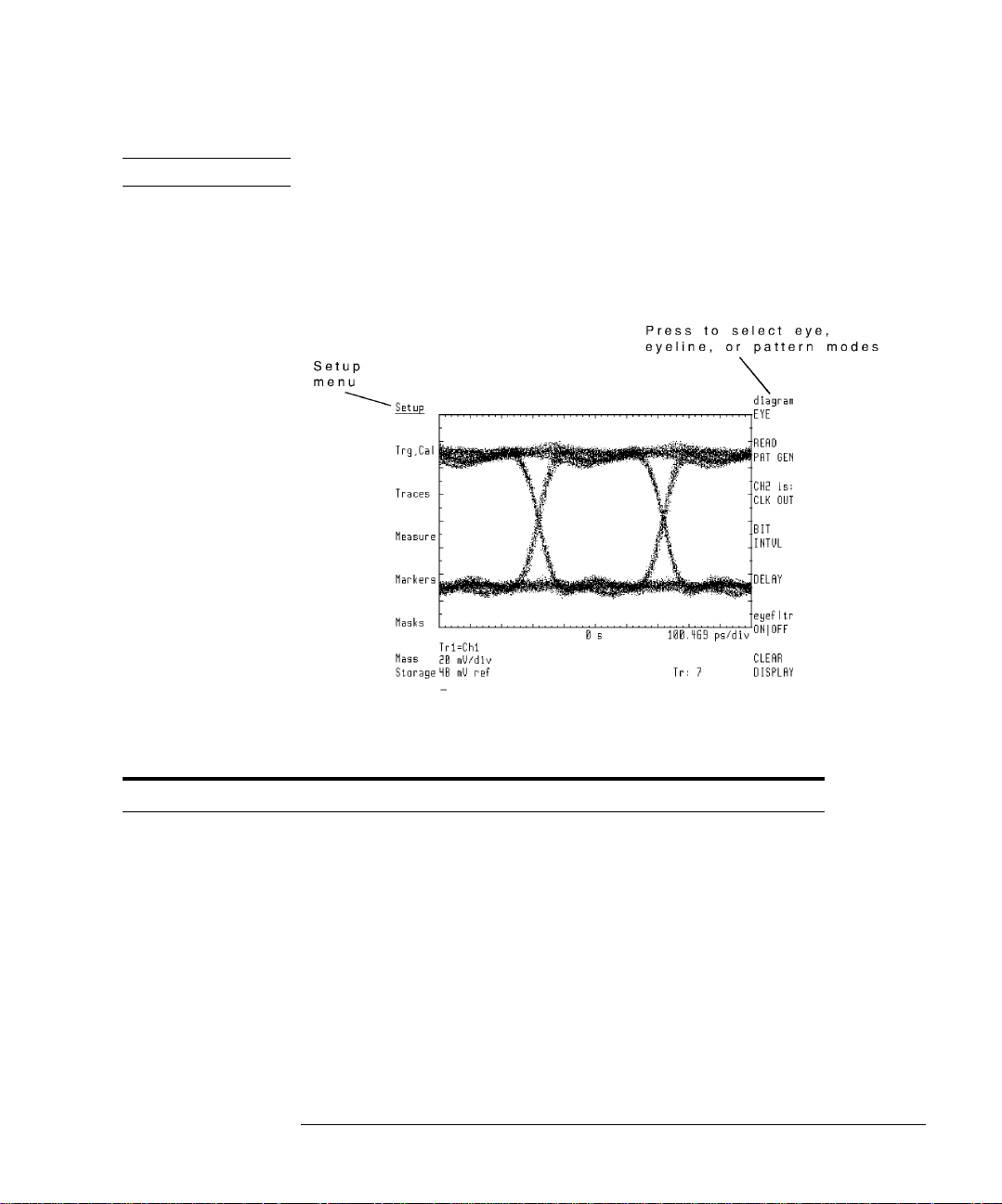
Select from eye, eyeline, and pattern modes

Use the Setup menu’s d iagram softkey to select from one of th re e measure- ment modes: eye, eyeline, and pattern.

Features Available in Each Mode

Eye Mode Eyeline Mode Pattern Mode

Eye Measurements X Extinction Ratio Measurements X X Mask Testing X X X Display the Mask Error Trace X X Improve Sensitivity Using Eye Filtering X X 40 GHz Extended Bandwidth X X User-Corrections X X Display Data Pattern X

1-5

Getting Started

Steps for Setting Up Eye-Diagram Analysis

Eye Mode The eye mode displays traces using individual dots in a manner that is similar

to conventional sampling oscillos c o pe s. Use this mode for the fol lowing:

• Typical eye-diagram measurements

• Extinction ratio measurements

Getting Started

Steps for Setting Up Eye-Diagram Analysis

Eyeline Mode : Eyeline mode disp la y s continuous traces. U se this mode for the following:

• Measure exti nc t i o n ratio

• Measure laser turn-on transition delay

• Examine laser overshoot

• Observe laser ringing

• Apply eye-filter

• Apply user-corre ctions

1-7

Getting Started

Steps for Setting Up Eye-Diagram Analysis

Pattern Mode Pattern mode displays the a c tual PRBS data strea m bits. This mode uses the

pattern trigger which allows the displ a y to show the same portion of the data stream from sweep to sweep.

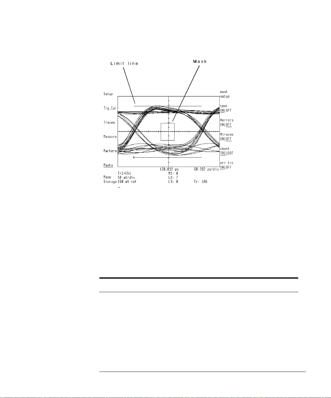
Mask/limit lines provide pass/fail testing

Mask/limit lines are displayed geometric shapes that define the accep table limits and shape of an eye -d ia gram. The following figure shows a mask. Use masks for pass/fail testing and as an aid to error analysis. The eye-diagram analyzer can capture and display the portion of the pattern that caused a mask violation. Built-in standard masks for the major SONET/SDH transmission rates are provided and can be applied with the press of a softkey. Or, you can create your own custom masks.

Getting Started

Steps for Setting Up Eye-Diagram Analysis

Apply software filters in eyeline mode

In eyeline mode, user frequency corrections can be appli ed to the data to simulate a hardware transmission filter. The eye-diagram analyzer comes with several Bessel-Thomson fil te rs. The se files are on the 71501D memory card. Refer toChapter 9, “Agilent 70820A: User Corrections” and Chapter 11, “Agi-

lent 70820A: Memory Cards, Disks, and RAM”for information on user-correc-

tions.

User Correction Files

File Name File Data

a_bt248832 4th order Bessel-Thomson filter for 2.48832 Gbit/sec transmission a_bt_62208 4th order Bessel- Thomson filter for 622.08 Mbit/sec transmi ssi on a_bt_15552 4th order Bessel- Thomson filter for 155.52 Mbit/sec transmi ssi on

1-9

Getting Started

Steps for Setting Up Eye-Diagram Analysis

Three sweep selections are available

• single

• continuous

• stopped

With the continuous selection, sweeps occur as soon as the selected triggering conditions are met and repeat continuously as long a s the trigg e r cond itions are met.

The source of the tri gg e r reference is selected using the Setup menu’s CH2 softkey. The following table shows the reference used when using an Agilent 7084X pattern generator.

Table 1-1.

Trigger Reference of 70841

Eye Mode

CLOCK

or TRIGGER CLOCK or TRIGGER TRIGGER

a. This connection provides faster trace updates.

Entering the pattern generator’s settings

The Setup menu’s READ PAT GEN softkey queries the 70841 patte rn g en er ator and 70311A signal generator for the clock freque ncy, pattern length, and any divide ratios. In the case of alternate configurations, an appropriate submenu will be displayed f or the param eters that require manual updating.

Note A READ PAT GEN should b e pe rformed after changing pattern generat or

settings, such a s c loc k frequency or patt e rn length.

Moving the measurement plane

Specifying an attenuation on channel 1 changes the measurem en t plan e fr om the front-panel RF INPUT 1 c onne ctor to include the indicate d attenuation. Specifying any attenuation on channel 2 may be necessary to ensure proper triggering. Use the Trg,Cal menu’s CH1 EXT ATTEN and CH2 EXT ATTEN softkeys to specify any external attenuation .

Getting Started

Steps for Setting Up Eye-Diagram Analysis

These softkeys can also be used to specify an optical-to-electrical responsivity conversion between the source and input channels. As a result, the display shows optical units referenced to the input of the optical-to-electrical converter. Channel and marker readouts change to watts/div. Also, the CH1 EXT A TTEN softkey changes to read CH1 RSPVTY (responsivity).

Autoranging

The Trg,Cal menu’s autorng ON OFF softkey turns on or off autoranging. When autoranging is activated, the eye-diagram analyzer automatically selects the appropriate hardware gain and offset to maximize the signal at the analogto-digital converter, regardless of the input signal’s amplitude.

Selecting the 10 MHz reference on Instrument Preset

Use the Trg,Cal menu’s IP REF softkey to select the source of the 10 MHz ref- erence on an INSTR PRESET. Choices are internal, external, or auto. With auto, the eye-diagram automatically selects an external refere nce if it is present at the 70820A’s rear-panel connector. Otherwise, the module’s inter- nal reference is selected.

Redefining the INSTR PRESET key

The Trg,Cal menu’s DEFINE U SE R IP so f tk ey redefines the settings invoked by the INSTR PRESET key. Redefini ng the instru ment preset can save valuable time when configuring for measurements.

1-11

70841A/B Pattern Generator and 70311A Signal Generator Modules

Getting Started

Steps for Setting Up Eye-Diagram Analysis

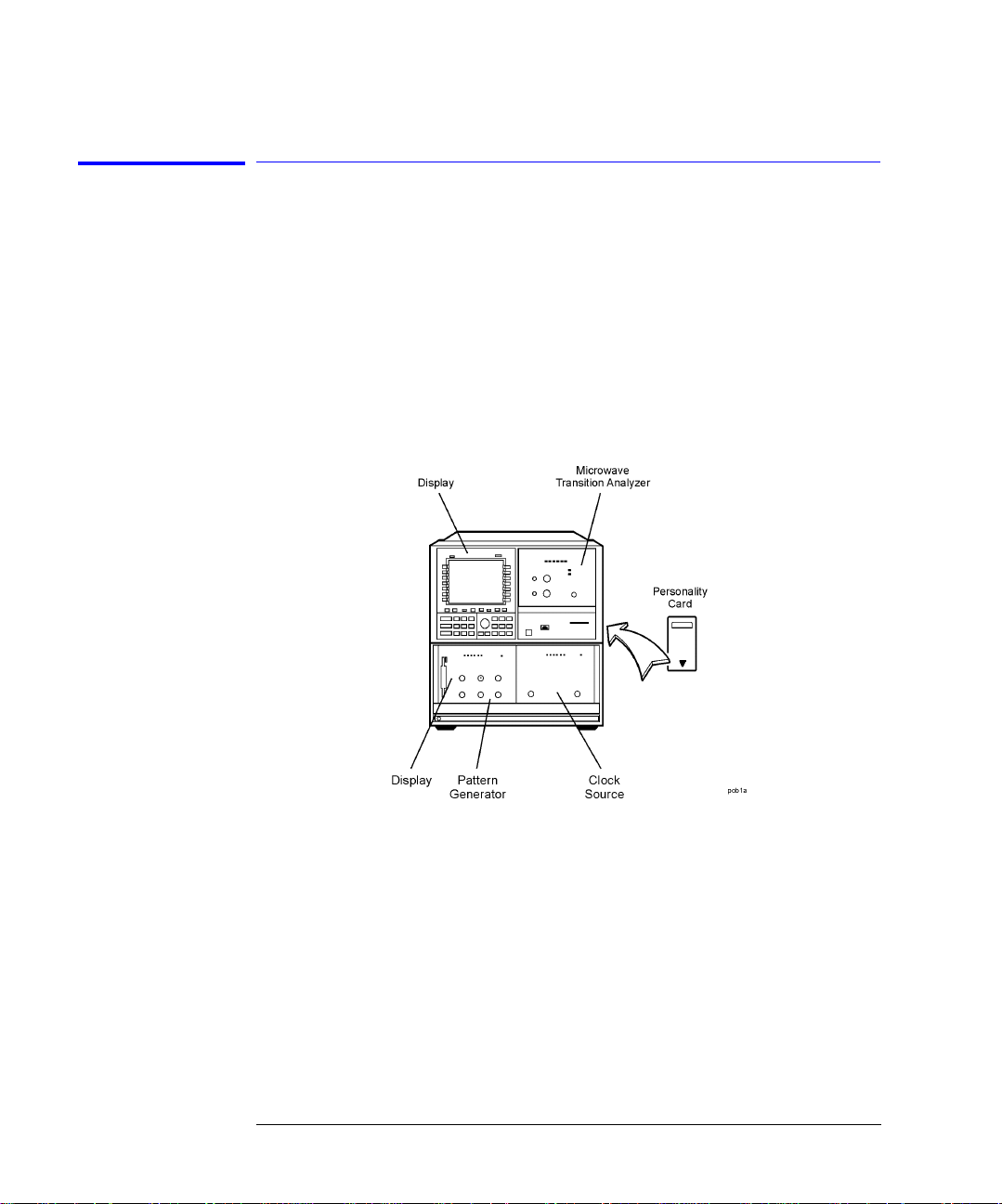
Step 1. Connect the Equipment

1 If you are using 70841A/B pattern generator and 70311A signal generator

modules with your eye-diagram analyzer, install them into an MMS mainframe as shown in the follo w in g figure.

Getting Started

Steps for Setting Up Eye-Diagram Analysis

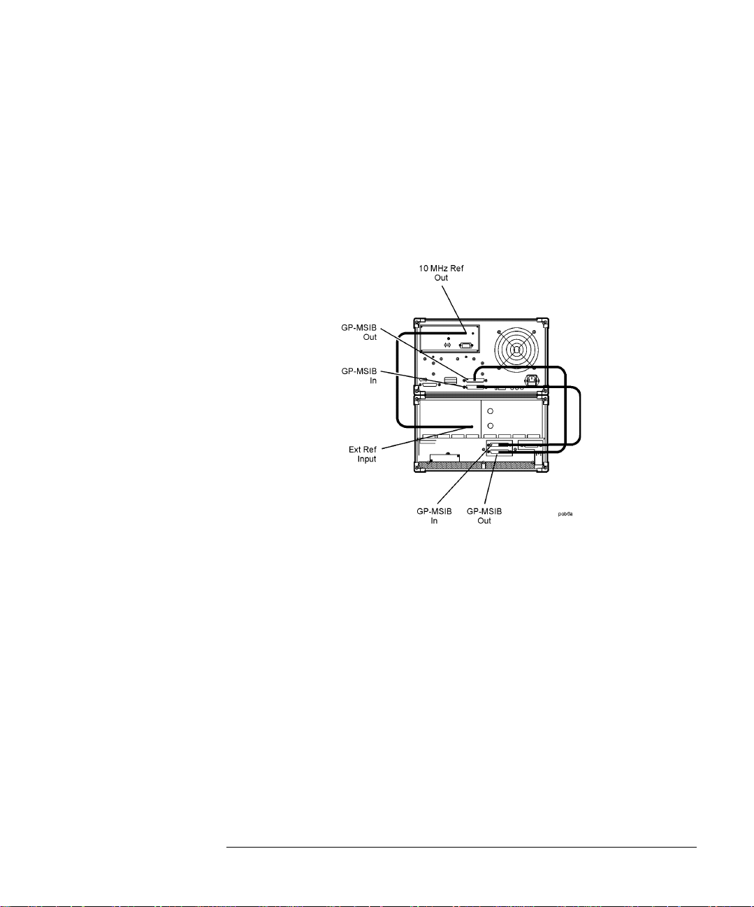
2 If you are using 70841A/B pattern generator and 70311A signal generator

modules with your eye-diagram analyzer, connect cables to the instruments as shown in the following graphic.

• If you are using a clock source other than an 70311A, make s ure that th e signal generator and 70820A microwave transition anal yze r modu le shar e the same frequency r eference. Use t he 10 MHz REF connecto rs on the rea r panel of the 70820A.

Rear-Panel Cable Connections

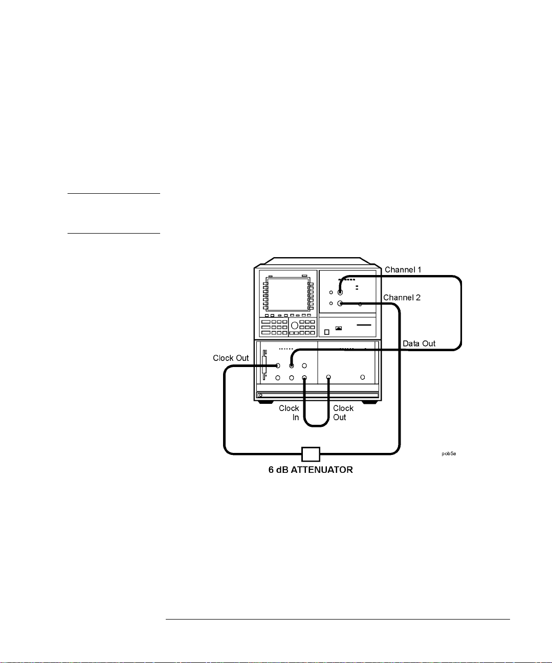
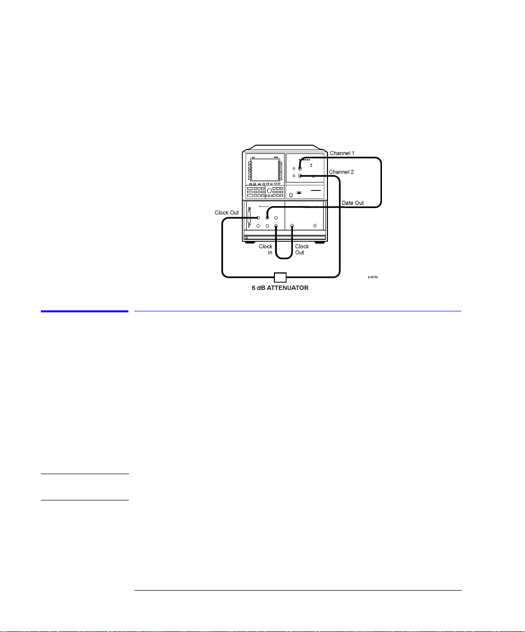
3 Connect the front -panel cables as show n i n the figure on the following page.

Use an adapter between the cables and channel connectors. The data signal connects to the 70820A’s RF INPUT 1 connector. The trigg er or clock signal connects to the 70820A’s RF INPUT 2 connector.

1-13

Getting Started

Steps for Setting Up Eye-Diagram Analysis

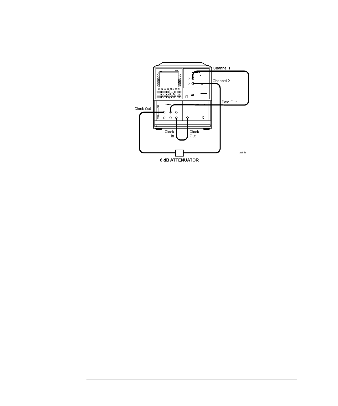
Front-Panel Cable Connections

Cables:

SMA to SMA (Channel 1) p/n 8120-4948 SMA to SMA (Channel 2) p /n 8120-4948 SMB to SMB (10 MHz Reference) p/n 8120-5025

Miscellaneous:

3.5 mm (f) to 2.4 mm (f) (two) p/n 1250-2277 6 dB attenuator 8493C

4 If the attenuator connected to the 70820A’s RF INPUT 2 connector is not 6

dB, press:

Trg,Cal, CH2 EXT ATTEN, then ente r the value of the attenuator

Getting Started

Steps for Setting Up Eye-Diagram Analysis

Laser and Opticalto-Electrical Converter

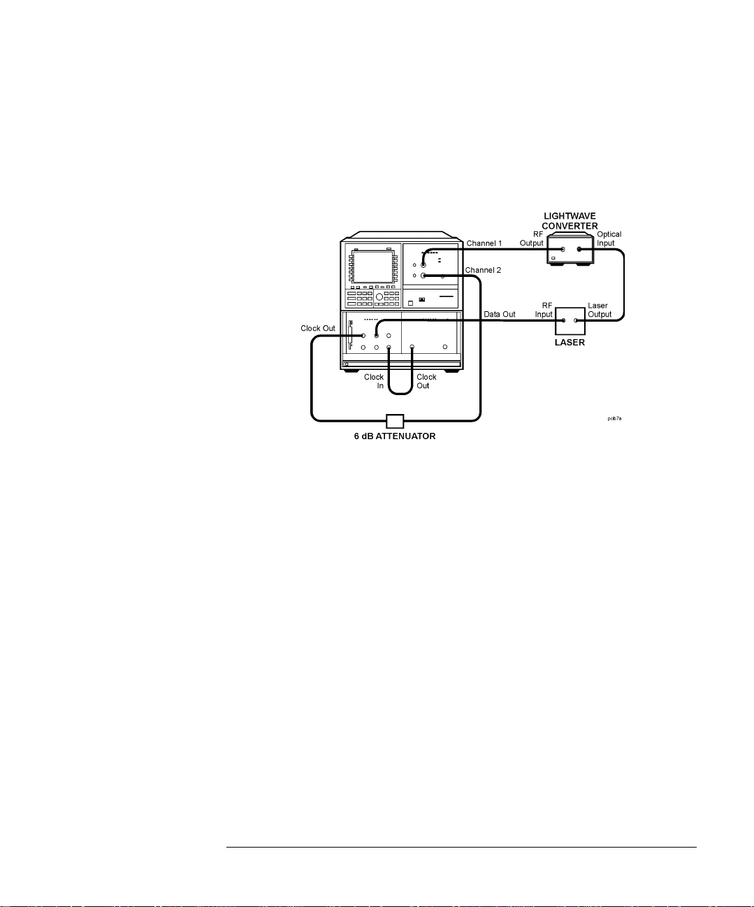
If you have access to a laser and an optical-to-electrical converter, use the connections shown in the following figure. To protect the input connectors, use adapters between the cables and the connectors. The laser i s the device being tested.

Cables:

SMA to SMA (Channel 1) p/n 8120-4948 SMA to SMA (Channel 2) p/n 8120-4948 SMB to SMB (10 MHz Reference) p/n 8120-5025

Miscellaneous:

3.5 mm (f) to 2.4 mm (f) (two) p/n 1250-2277 6 dB attenuator 8493C

1-15

Getting Started

Steps for Setting Up Eye-Diagram Analysis

Connections without a Laser Source and Converter

Automatically Load the Personality

If a laser source and optical-to-electrical converter are not available, use th e alternate connec tion shown in the following figure. In this c a se, the pattern generator’s data output is displayed. An electrical device could be inserted between the pattern ge nerator and the eye-diagram analyzer.

Step 2. Load the Personality

1 Insert the eye-diagram personality card into the front-panel card slot of the

microwave transition analyzer, facing the metal strip on the card downward and toward the inst rument. Make sure the ca rd is fully inserted into the card slot.

2 Switch on the power to all of the equipment. Switch on the power to the

70820A last. The start up process takes about 6 minutes.

Note Do not press any instrument keys until the program is loaded. Pressing keys

can cause the automatic program loading to abort.

Getting Started

Steps for Setting Up Eye-Diagram Analysis

If the Program Failed to Load

The program has failed to lo ad if one of the following occurs:

• The message Please wait... Loading 70874 never sho w s.

• The left-side softkeys match those shown in the followin g figure.

“Manually Load the Personality” on page 1-17

Manually Load the Personality

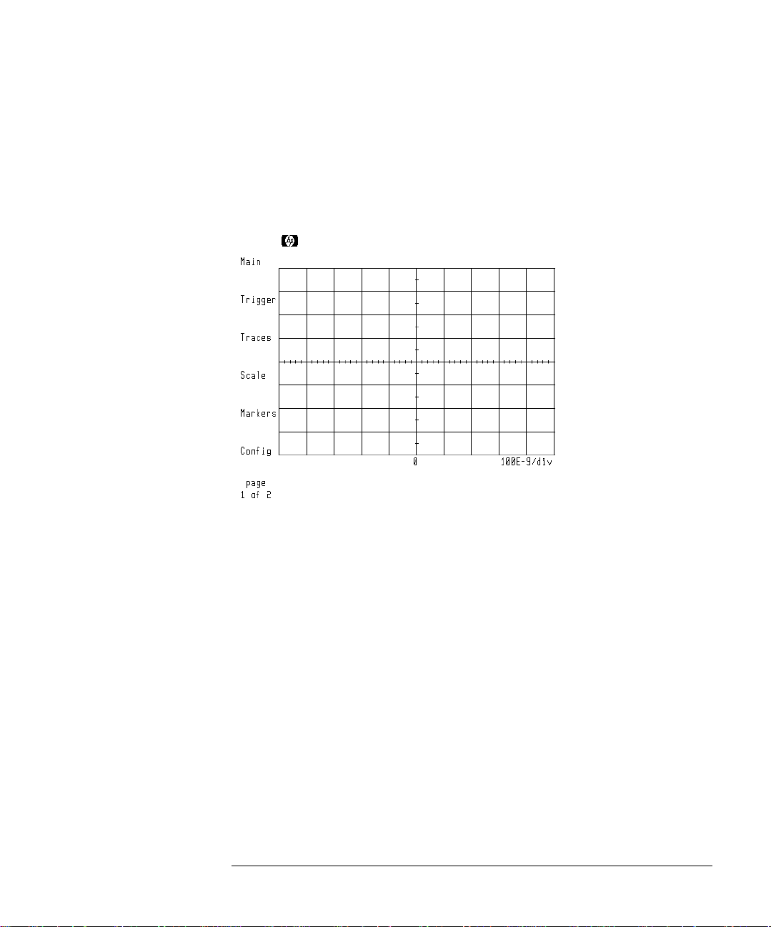
70820A Module’s Main Menu

1 Insert the 70874A eye-diagram memory card into the front-panel card slot. 2 Display a listin g of the files on the memory card by pressing:

MENU, page 1 of 2, States, more 1 of 2, mass storage

1-17

Getting Started

Steps for Setting Up Eye-Diagram Analysis

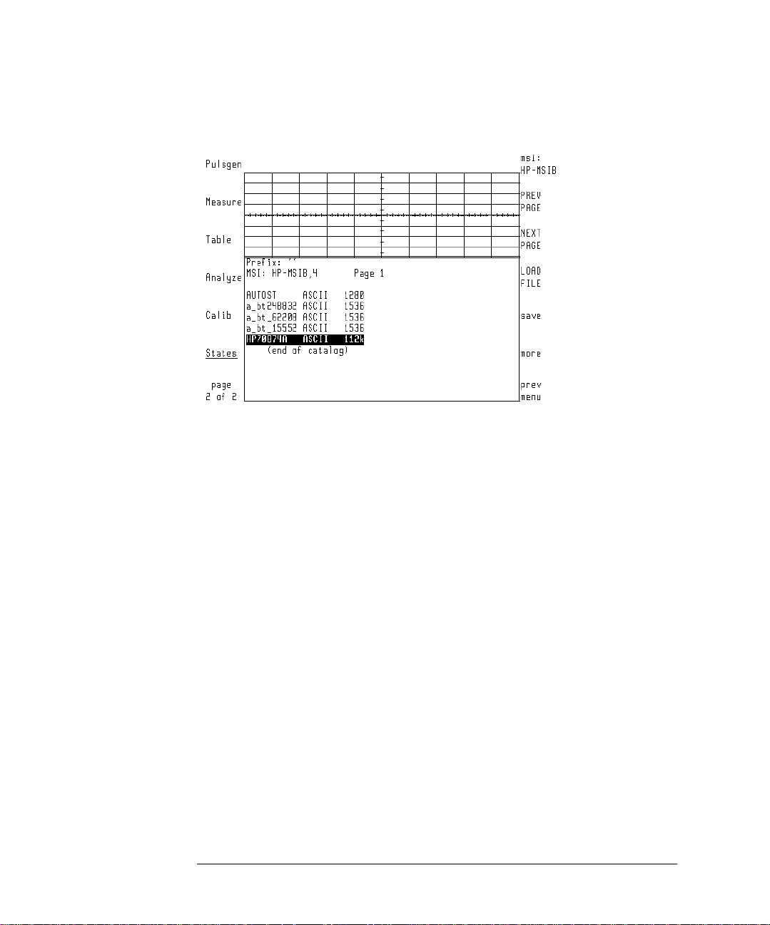
3 If the screen does not resemble the above figure, press:

msi:, HP-MSIB CARD, prev menu

DISPLAY, Mass Storage, msi, MEMORY CARD MENU

The list of files should now be displayed.

4 Turn the front-panel knob to highlight the file "AUTOST" and then press:

LOAD FILE

If you load the "70874" file by mistake, the message 7386 memory overflow may be displayed. This error message is a result of the manual loading pro-

cess and, in this instance, does not indicate a problem. The program still should be properly loaded.

Getting Started

Steps for Setting Up Eye-Diagram Analysis

Step 3. Complete the Installation Using the Screen Instructions

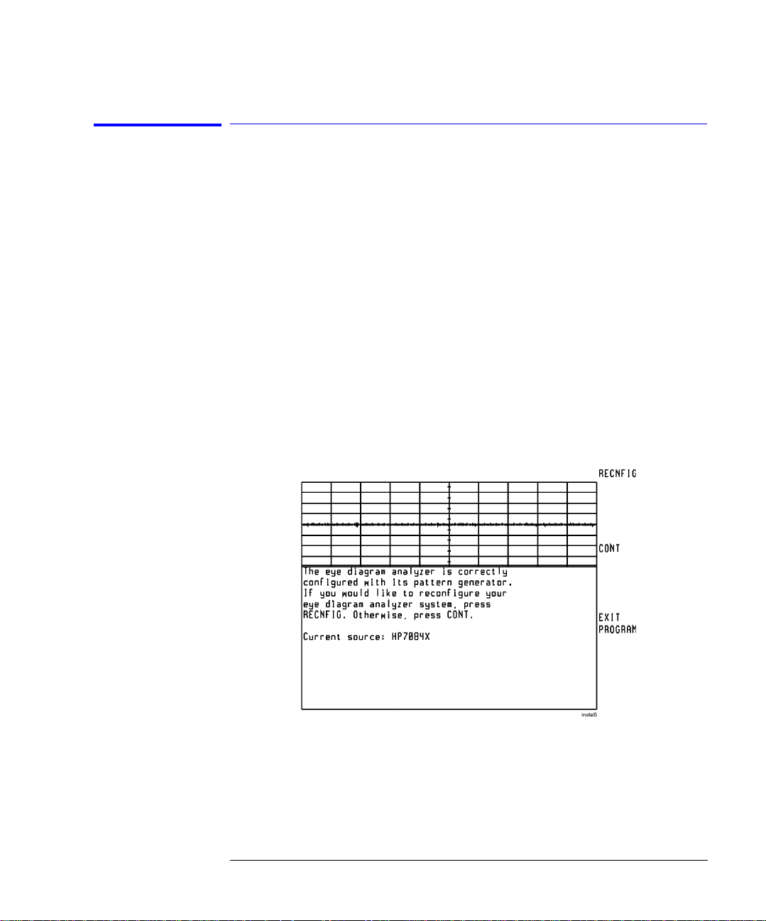
• If the displayed screen looks like the figure on the left side of this page, your system has been previously configured. Press CONT a nd the n c ontinue with "Step 4. Connect the front- pane l cab les". However, if you wish to reconfigure your system, press RECNFIG, and continue with the following explanation of the self-guided scree ns.

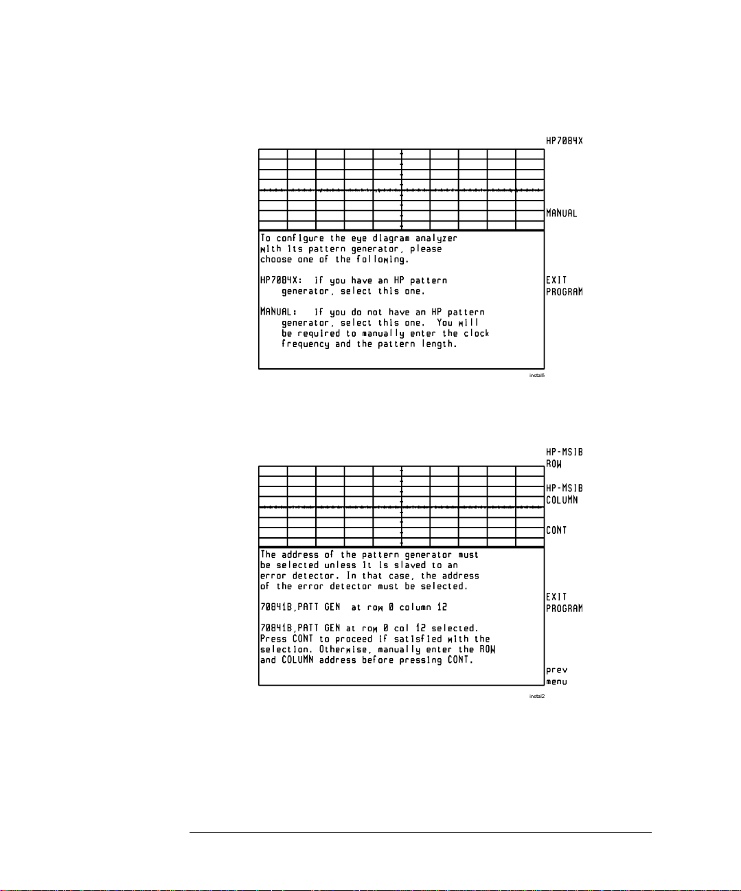
• If the screen looks like the figure on th e right side of this page, the first selfguided screen is displayed. Perform the following steps:

1 Press 7084X if you are using an 70841A/B pattern gener ator. If using an

70843A, or any other pattern generator, press MANUAL.

2 If you press 7084X, the screen shown on the following page is displayed. The

program automatically determines and displays the pattern generator module’s HP-MSIB addres s. For most installations, press CONT. To m a nually enter the HP-MSIB address , use the displayed softkeys.

Example of a Configuration Previously Done

1-19

Getting Started

Steps for Setting Up Eye-Diagram Analysis

First Self-Guided Screen

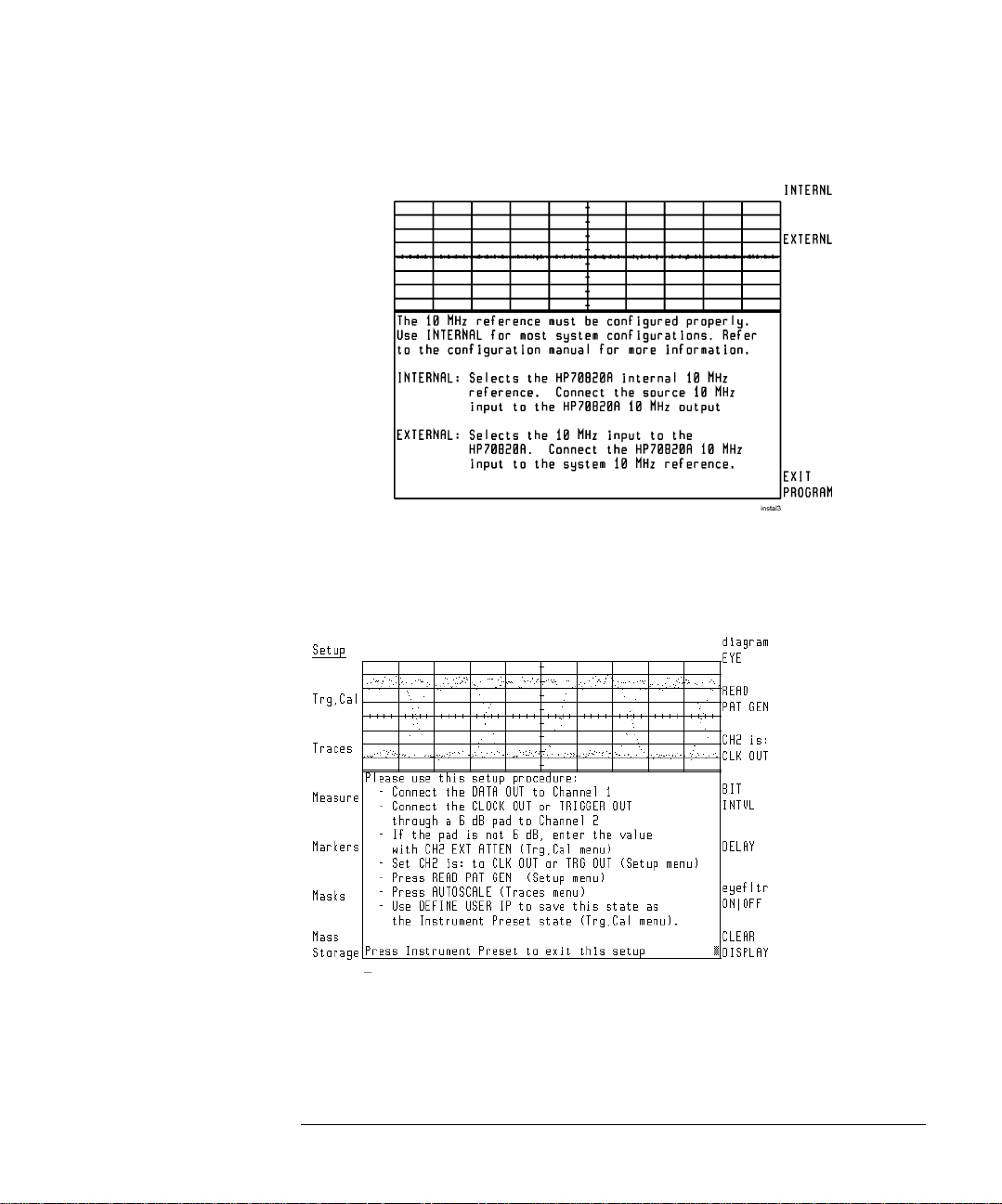
3 Use the following self-guided screen to indicate the 10 MHz frequency

reference used. Press INTERNL if the 70820A module is used as the reference. Press EXTERNL if the clock source is used as the reference.

Getting Started

Steps for Setting Up Eye-Diagram Analysis

4 The following screen should be displayed. Notice that the eye-diagram

analyzer’s left-side Setup menu is selected.

5 If you have not already connect the cables to the instruments’ front panels,

follow the instructions shown. Otherwise, proceed with “If you have not already

connect the cables to the instruments’ front panels, follow the instruct ions shown. Otherwise, proceed with “If you have not already connect the cables to

1-21

Select the Mode

Select Single or Continuous Sweeps

Getting Started

Steps for Setting Up Eye-Diagram Analysis

the instruments ’ front panels, follow the instructions shown. Otherwise, proceed with “If you have not already connect th e cables to th e inst rume nts ’ front panels, foll ow the instruction s shown. Otherwise, proceed with “If you have not already connect the cables to the instruments’ front panels, f ollow the instructions shown. Otherwis e, proceed with .” on page 1-21.” on page 1- 21. ” on page 1-22.” on page 1-22.

Step 4. Set Up the Measurement Conditions

1 To select the mode , press:

Setup, diagram, EYE, EYELINE, or PATTERN

2 Press the left-sid e Trg,Cal softkey.

Select Trigger Source

3 Select one of the following sweep states:

• Press SINGLE to select single sweeps. Each additional press of this softkey triggers another sweep.

• Press CONT STOP CONT

• Press CONT STOP STOP

4 Press the left-sid e Setup softkey. 5 Press CH2.

• If the pattern generator’s CLOCK OUT signal is connected to the RF INPUT

2 connector, press CLK OUT.

• If the pattern generator’s TRIGGER OUT signal is connected to the RF IN-

PUT 2 connector, press TRG OUT.

to select contin uous sweeps.

to stop the sweeps.

Getting Started

Steps for Setting Up Eye-Diagram Analysis

Note Using the CLOCK OUT trigger si gnal provides faster data acquisitio n for eye-

diagrams. If the amplitude of the trigger signal is too large, an over-range message is disp layed. If a message is displayed, reduce the amplitude of the signal; use an external attenuator, and enter the value using CH2 EXT ATTEN.

Select the Patt ern Generator Settings

6 If an 70841A/B pattern generator is used, press READ PAT GEN. 7 The eye-diagra m a n alyzer reads the settings of the pattern ge nerator. 8 If a pattern generator, such as the 70843A/71612A , is used in place of an

70841A/B pattern generator, press:

READ PAT GEN, CLOCK RATE and enter the rate of the clock signal CLOCK DIVISOR and enter the divisor for the clock signal

For example, whe n us ing a trigger or sync ou tput, enter 16 if the clock signal is divided by 16.

9 Enter the pattern repetition length by pr essing:

PATTERN LENGTH and enter the pattern repetition length

The pattern repetition length is entered in bits or as the binary power depending on the position of the 2^n-1 ON OFF softkey. If the function is on, binary powers are ent ered in the f orm 2

–1. This makes it very easy to set the pattern length for PRBS sequences. When the function is off, the pattern length is entered directly in bits.

10 Press PAT TRG FACTOR, and enter the factor that relates how many

repetitions of the pattern occur between trigger pulses . Frequently, 16 to 32 or more repetitions of the pattern occur between trigger

pulses.

Note When operating off a trigger or sync output with a divided clock frequency or

a pattern trigger, be sure to set CH2 is: to TRG OUT.

11 If a signal generator other than the 70311A is use d, ente r the pr eci se clock

frequency by pres sing:

prev menu, CLOCK RATE and enter the clock rate

1-23

Getting Started

Steps for Setting Up Eye-Diagram Analysis

Controlling an 70841A/B Pattern Generator

When using the 70311A clock source (below 3 Gb/s):

This section explains how to display the menus for the 70841A/B pattern generator. The display can be assigned to control either the eye-diagram analyzer or the 70841A/B pattern generator.

Note If the eye-diagram analyzer is conf igured with a non 70841 pattern gene rat o r,

you must manually set the trigger level. Refer to “To Manually Set the Trigger

Level” on page 1-25 in this c ha p ter.

1 Turn on the power fo r both mainframes. Wa it until the start-u p ro utines are

completed and the mainframes are ready for key presses.

2 Continue by pressing :

DISPLAY, NEX T INSTR

If several instrum ents are in the system, you may have to press NEXT INSTR several times.

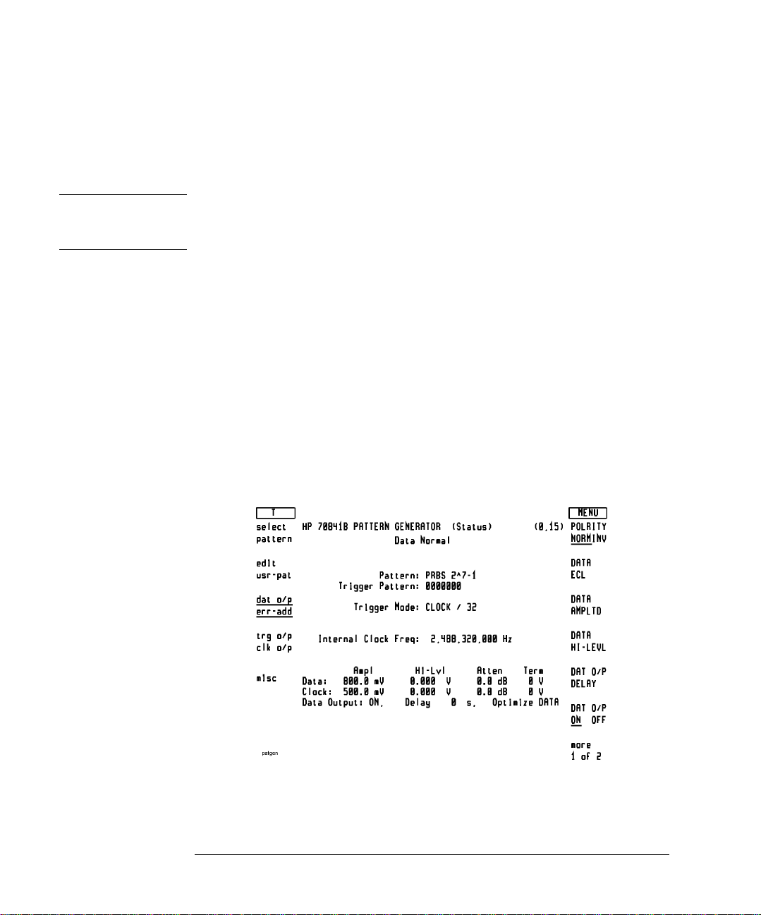
3 If the 70841A/B’s status screen , shown in th e following figure, is not shown, the

pattern generator is probably addressed as a slave instead of a master. Perform the following steps:

a Press the left-side Address Map softkey.

An Example 70841A/B’s Status Screen

b Use the front-panel knob to scroll the box to the column where the

Getting Started

Steps for Setting Up Eye-Diagram Analysis

70841A/B appears.

c Press ADJU ST ROW, and rotate the knob to move the box to the row where

the 70841A/B appears.

d Press ASSIGN BOTH.

4 Use the displayed softkey menus to set the pattern generator to the desired

settings. For an exa mple, refer to the paragraph "Configure the data signal" in

Chapter 2, “Applicatio n Tutorials”.

5 To return control to the eye-diagram analyzer, press:

DISPLAY, NEXT INSTR

6 To return to the eye-di a gram analyzer personality menus, press:

USER

To Manually Set the Trigger Level

If a pattern generator other than the 70841A/B is used, you must use the following procedure to manually set the tri gger level.

1 Select trace two an d turn the display on by pressing:

> prev menu, select:, TR2, display ON/OFF ON

2 Automatically scale the trigger trace and set the trigger level by pressing:

AUTO-SCALE, Trg,Cal, LEVEL

Use the knob to position the trigger level indicator line so it crosses an edge.

1-25

Getting Started

Steps for Setting Up Eye-Diagram Analysis

3 Turn the display off and sele ct tr ace one by pressing:

Move the Measurement Plane

Traces, display ON|OFF OFF

To move the measurement plane, press:

Trg,Cal, CH1 EXT ATTEN and enter the attenuati on on channe l 1 in put .

, select:, TR1

Optional Step. Save Instrument State as Preset State

1 Select the Traces menu and scale the screen to the displayed signal by

pressing:

Traces, AUTOSCALE

2 Save the current instrument state by pressing:

Trg,Cal, more 1 of 2, DEFINE USER IP, CONT

The current instrument state is sav ed, including the pattern generator’s HPMSIB address, th e frequency referen c e, scaling, and trig ger level. Whenever INSTR PRESET is pressed, the eye-diagram analyzer is automatically placed in these settings.

3 The eye-diagram i s now re ady for use.

Getting Started

Steps for Setting Up Eye-Diagram Analysis

To restore the factory instrument preset

Restore the fact o ry instrument preset b y pressing: MENU, page 1 of 2, States, more 1 of 2, preset: FAC|USR FAC

1-27

Getting Started

Steps for Setting Up Eye-Diagram Analysis

Application Tutorials

Application Tutorial s

Application Tutorials

This chapter contains nine tutorials that in troduce important eye-diagram analyzer feat ur es. The tutorials should be performed in the order listed . To create the data signal, you will need a pseudo-random binary sequence (PRBS) pattern generator. Refer to “Configure the Data Signal” on page 2-2 before you start the tutorials. You will find the following topics in this chapte r:

• Tutorial 1: Measure Eye-Parameters 2-4

• Tutorial 2: Measure in Optical Power Units 2-8

• Tutorial 3: Measure Extinction Ratios on Low-Le vel Signals 2-10

• Tutorial 4: Measure Laser Turn-on Delay 2-13

• Tutorial 5: Use Software Filters 2-15

• Tutorial 6: Test to Industry Standards 2-19

• Tutorial 7: Default and Custom Mask or Limit Line T esting 2-23

• Tutorial 8: Display the Data Pattern 2-27

• Tutorial 9: Constructing a Low-Pass Filter from a Transfer Functi on 2-30

• Tutorial 10: Create a Vertical Histogram 2-36

• Tutorial 11: Create a Horizontal Histogram 2-41

Configure th e Dat a Sign a l

The following li st shows typical settings that can be used for the data signal. The list assumes you are using an 70841A/B pattern generator. The exact settings depend upon the system you are using. If the system includes an 70841A/B pattern generator, use the pattern generator’s status screen to enter these values. The procedure for viewing the status scree n is e xplained in

“Controlling a n 70 841A/B Pattern G enerator” on page 1- 24.

• In the select pattern menu:

Pattern: PRBS 2^7-1

• In the dat o/p err-add menu: Data Ampl: typically 800 mV to 2 V (depending on laser) Data Hi-Lvl: 0 V (d epending on laser)

• In the trg o/p clk o/p menu:

Application Tutorials

Clock Freq: 2.48832 GHz Clock Ampl: 500 mV Clock Hi-Lvl: 0 V

If you’re performing these tutorials without the laser source and optical-toelectrical converter, reduce the level of the data signal as shown in the following settings :

• Data Ampl 250 mV

• Data Hi-Lvl 300 mV

2-3

Application Tutorials

Tutorial 1: Measure Eye-Parameters

The eye-diag ram analyzer performs automatic eye measurements in eye mode. This mode is similar to that of conventional sampling oscilloscopes; the display shows individual dot s.

View the Signal

1 To view the signal, press:

INSTR PRESET, Traces, persist, VARIABL

This turns the persi stence mode on. Refer to Chapter 3, “Eye-Diagram Ana-

lyzer Reference” for an explanation of the available persistence modes.

2 Enter the number of sw eeps by pressing:

PERSIST SWEEPS and enter 8

3 Turn autoscalin g on by pressing:

prev menu, AUTO-SCALE

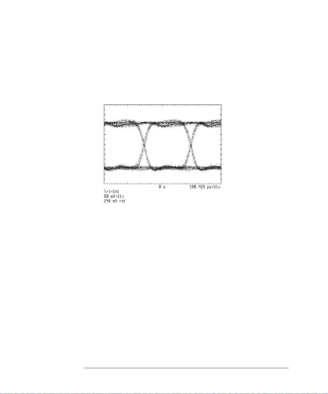
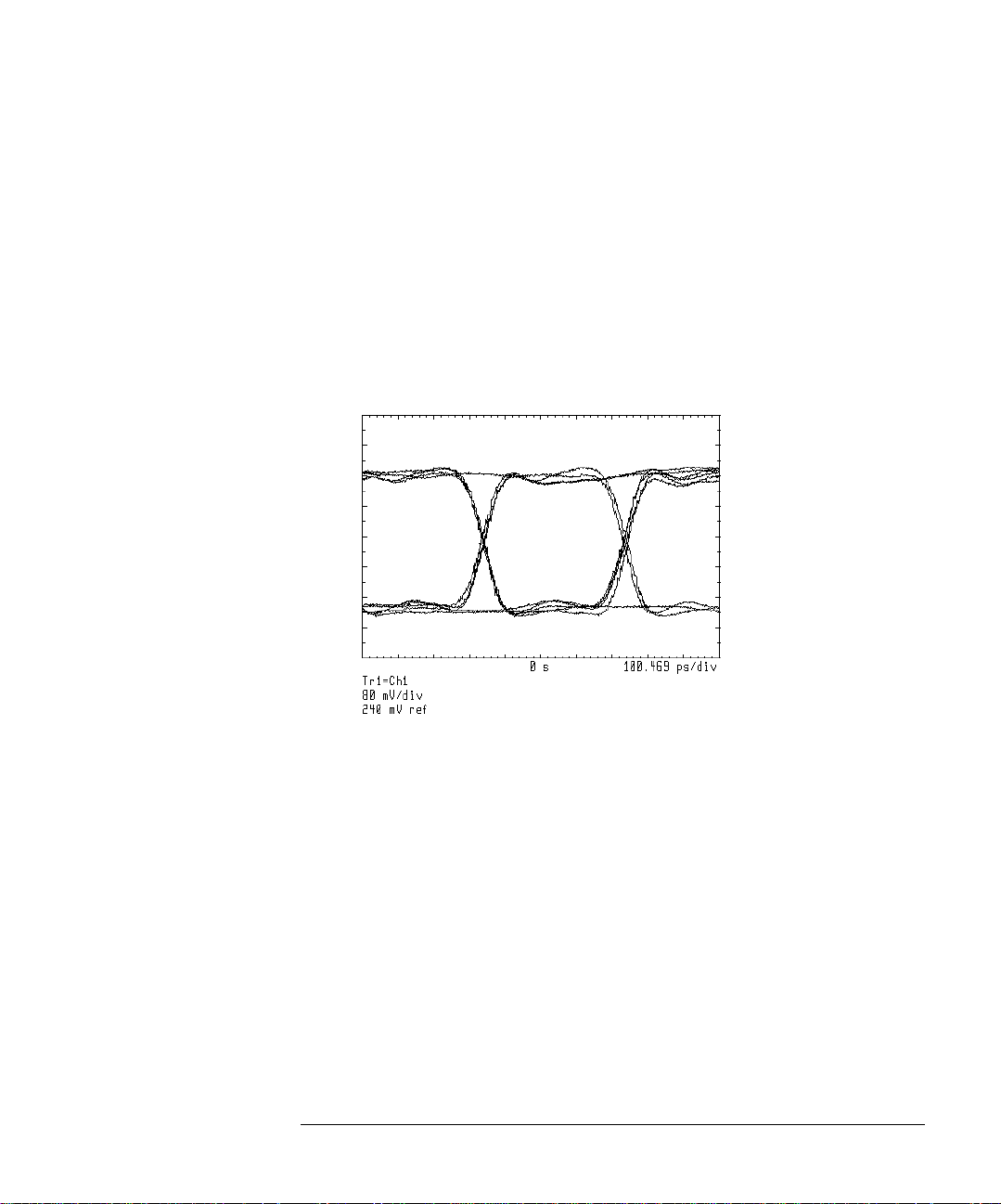
The display should look simila r to the display of a sampling oscilloscope . See the following figure.

The large overshoot shown is a result of the particular laser bias setting used. If the edges of the waveform are unstable in time (indicating no trigger), refer to the “T o Man u a lly Set the Trigger Level” on page 1-25.

Tutorial 1: Measure Eye-Parame ters

Example of a Large Overshoot Resul t i ng f r om Laser Bias

Application Tutorials

Perform an Offset Calibration

This calibrati on procedure re mo v es any offset that ma y be present in the optical-to-electrical converter. This is sometimes referred to as the "dark" level. The offset calibration ensures accurate measu rem en ts of the laser’s one a nd zero levels .

4 Turn the laser off . (If yo u a re measuring the pat tern generator directly,

disconnect the input signal at channel 1.)

5 Perform the ca libration by pressing:

Trg,Cal, OFFSET CAL, CONT

The calibration takes about a minute to execute. When th e ca libration is finished, DC NULL: done is displayed.

6 Turn the laser on. (I f yo u are measuring the pattern generator directly,

reconnect the input signal at channel 1.)

Measure Signal Parameters

7 To include the rise time and fall time measurement in the displayed results ,

press:

Measure, r/f tim ON OFF ON

2-5

Application Tutorials

Tutorial 1: Measure Eye-Parameters

Enabling this function approximately doubles the meas urement time.

8 Perform the eye measurement by pressing:

MEASURE EYE

After a brief period of time, the display should look like the following figure. Refer to Chapter 3, “Eye-Diagram Analy zer Reference” for definitions of each measurement listed on the screen.

Example Eye Measurements

Measure Extinction Ratio

9 Measure the extinction ratio by pressing:

EXTINCT RATIO

The results are added to the displayed list of measurement results.

Tutorial 1: Measure Eye-Parame ters

Example Extinction Ratio Measurement

10 Change the amount of data used for the hi stograms by pressing:

NUMBER SAMPLES and enter the # of samples

Application Tutorials

A larger value gives more accuracy, but increases the data acquisition time. When making extinct ion ratio measurem ents in eyeline mode, the number

of samples should be increased from the default of 1000 to something on the order of 20000 to insure a number of traces are evaluated to compute the extinction ratio.

11 Clear the measured data from the screen by pressing:

OFF

2-7

Application Tutorials

Tutorial 2: Measure in Optical Power Units

The analyzer display has the ability to show optical units referenced to th e input of the optical-to-electrical converter. This changes the channel and marker readouts to watts/div.

1 Set the analyzer to a known state by pressing:

INSTR PRESET, Trg,Cal, CH1 EXT ATTE N responsivity val u e, V/Watt

For example, th e following figure show s 350 V/Watt entered. Notice th e softkey label changes to CH1 RSPVTY (responsivity) .

2 To use the markers to read optical power, press:

Markers, Y1 (--)

3 Adjust the m arker l ine to th e p eak o f t he r es pons e. For examp le, t he f ollow i ng

figure shows a peak optical power of 1.5 mW.

Application Tutorials

Tutorial 2: Measure in Optical Power Units

2-9

Application Tutorials

Tutorial 3: Meas ur e Extinction Ratios on Low-Level Si gnals

Tutorial 3: Measure Extinction Ratios on LowLevel Signals

Repeatable extinction ratio measurements can be made on low-level signals. This is accomplished by applying a filter to the signal. This filter improves measurement sensitivity and is useful for analyzing:

• low-level extinction ra ti os

• pattern dependent trans it ion s

• intersymbol interference

In this tutorial, the eye-diagram analyzer is placed in eyeline mode so that the eye filter can be applied to reduce trace noise. T o measure the signal, a photodiode converter with a responsivity of 30 volts/watt is used.

When making extinct ion ratio measurem ents in eyeline mode, the number of samples should be increase d from the default of 1000 to something on the order of 20000. This insures a number of traces are evaluated to compute the extinction ra tio. The compatible mode is eyeline .

Change to Eyeline Mode

1 Set the instrument to a known state by pressing:

INSTR PRESET, Setup, diagram, EYELINE, Traces

2 Set the number of persistence sweeps by pressing:

persist, VARIABL, PERSIST SWEEPS and enter 5, prev menu

3 Turn on autoscaling by pressing:

Trg,Cal, more 1 of 2, Trac es, AUTO-SCALE

The display should look like the following figure. A low-amplitude response, similar to that shown in this figure, can result when

using non-amplified lightwave converters to measure opti cal sig nals.

Tutorial 3: Measure Extinction Ratios on Low-Le vel Signals

Autoscaled Display of Low-Level Signal

4 Turn filtering on b y pressing:

Application Tutorials

Setup, eyefltr ON OFF ON

Perform an Offset Calibration

5 Turn the laser off . (If yo u a re measuring the pat tern generator directly,

disconnect the input signal at channel 1.)

6 Perform the ca libration by pressing:

Trg,Cal, OFFSET CAL, CONT The calibration takes about a minu te to execute. When th e ca libration is

finished, DC NULL: done is displayed.

7 Turn the laser on. (I f yo u are measuring the pattern generator directly,

reconnect the input signal at channel 1.)

2-11

Application Tutorials

Tutorial 3: Meas ur e Extinction Ratios on Low-Level Si gnals

Measure the Extinction Ratio

8 To measure the extinc tion ratio, press:

Measure, NUMBER SAMPLES and enter 20000, EXTINCT RATIO

Refer to the follo wing figure.

Extinction Ratio Measurement on a Low-Level Signal with Eye Filtering On

Display the Signal in Optical Units

9 To display the signal in optical units, press:

Trg,Cal, CH1 EXT ATTEN and enter 30 V/Watt

Application Tutorials

Tutorial 4: Measure Laser Turn-on Delay

On-screen markers can be used to measure both amplitude and time separ ation in eye-diagrams. The compatible modes for markers a re eye, eyeline, and pattern.

Change to Eyeline Mode

1 Change to eyeline mod e, then turn filtering on by pressing:

INSTR PRESET, Setup, diagram, EYELINE, eyefltr ON OFF ON BIT INTVL and enter 1

2 Set the persistence to i nfinite by pressing:

Traces, persist, INFINIT, Trg,Cal

3 After several tra c es have been display ed, press:

CONT STOP STOP

Turn on the markers

4 Press X1 and X2 to activate markers 1 and 2. 5 Turn the front-panel knob to move the markers to different transition crossing

points on the waveform as show in the following figure. This provides an easy method to check the peak-to-peak difference in the laser

turn-on time measured at the crossing point. Notice in the fo llowing figure, a delta reading of 30 ps is displayed at the to p of the sc re en.

2-13

Application Tutorials

Tutorial 4: Measure Laser Turn-on Delay

Laser Overshoot and Turn-On Delay

Application Tutorials

Tutorial 5: Use Software Filters

This tutorial enables a software filter. The filter is designed with user frequency correcti o ns. User frequency corrections can be used for:

• Removing the effects of frequency response roll-off due to the optical-toelectrical converter and cables.

• Simulating hardware filters recommended for l ase r transmitter evaluation, such as 4th-order Bessel- Thom son filters.

The eye-diagram analyzer mus t b e in eyeline mode to a ppl y user-corrections. In eyeline mode, each sweep produces a continuous trace with the points connected. (This is opp o sed to unconnected dots with the eye mode.) Eyeline mode is especially useful for measuring variations in laser turn-on delay, overshoot, and ringing and for a ppl ying user frequency corrections. The compatible mode is eyeline.

Several Bessel-Thomson software filters are included on the 70874A eye-diagram analyzer’s memory card. These filters can be applied as user-corrections in the eyeline and pattern modes. (User corrections must be off in eye mode.) User correction files are identified by the prefix a_ as shown in the following table. Two addition al files on the card, AUTOST and 70874, comprise the eyediagram analyzer program.

Supplied User-Correction Files

File Name File Data

a_bt248832 4th order Bessel- Thomson filter for 2.48832 Gbit/sec transmiss ion. a_bt_62208 4th order Bessel- Thomson filter for 622.08 Mbit/sec transmi ssi on. a_bt_15552 4th order Bessel- Thomson filter for 155.52 Mbit/sec transmi ssi on.

2-15

Application Tutorials

Tutorial 5: Use Software Filters

User-Corrections Applied to the Data

Change to Eyeline Mode

1 Set the analyzer to a known state by pressing:

INSTR PRESET, Traces, persist, VARIABL and enter 5, diagram,

EYELINE

Notice the level of the las er ov er shoot, and the turn-on delay, varies from sweep to sweep, dependent on the previous pattern of ones and zeros.

Eyeline Display Showing Laser Overshoot

Load the Software Filter

Application Tutorials

Tutorial 5: Use Software Filters

2 Place the 70874A memory card in the front-panel card slot. 3 Display the catalog of files on the memory card by pressing:

Mass Storage

4 Turn the front - p anel knob to highlight the file "a_bt248832". 5 Load the file into user-corrections by pressing:

LOAD FILE This file simulates a 4th-order Bessel-Thomson filter with a cutoff at threequarters of the bit rate. This allows you to observe the laser transmitter signal in a specified bandwidth. This software filter is equivalent to using a hardware filter, except that trace nois e m a y be suppressed more .

6 Apply the filter data to the traces by pressing:

Trg,Cal, more 1 of 2, usr cor ON OFF ON

2-17

Application Tutorials

Tutorial 5: Use Software Filters

7 Turn the autoscale function on b y pr essing:

Traces, AUTO-SCALE

The display should look like the following figure. Notice that the laser overshoot is no longer visible, due to the filtering effect of

the user-corrections in the 71501A.

Example Filtered Laser Overshoot

Application Tutorials

Tutorial 6: Test to Industry Standards

Masks allow you to test eye-di a g ram s ag ainst industry standards. Th e eye-diagram analyze r provides built-in m a sks for testing the m a jo r SONET/SDH transmission rates. Compatible modes are eye and eyeline. Shown in this tutorial is the ability to:

• Count mask errors

• Allow for specified amount of margin testing

• Stop after a specif ie d num ber of trace errors

• Show the violation trace (eyeline mode only)

Select the Mask

1 Set the analyzer to a known state by pressing:

INSTR PRESET

2 You can use your own hardware filter during this tutorial, or load a software

filter as described in the previous tutorial.

3 Set the bit interval and delay by pressing:

Setup, BIT INTVL and enter 1.5, DELAY

Adjust the delay to center the eye.

4 Select a mask by pressing :

Masks, mask setup, default masks, STM-16 OC-48

The display shows an unscaled rectangle mask.

5 Align the mask by pressing:

MASK ALIGN Wait for the displayed # samp count to reach 100%.

This step aligns the mask to the data using automatic scal ing. Notice that, for the purposes of clarity, the graticule is tur n e d o ff. Th i s w as done using the 70820A Config menu.

2-19

Application Tutorials

Tutorial 6: Test t o Industry Standar ds

Turn Mask Testing On

6 Turn mask testin g on by pressing:

Masks, test ON OFF ON

This resets the error counters. Errors for the standard specifications show up beside the M1 screen annotation for mask violations, and beside L2 and L3 for upper and lower li mit violations , respectively .

Notice that in this case, violations are occurrin g due to too much overshoot.

Test with Additional Margin

7 Set a 15% mask margin and turn margin testing on by pressing:

mask setup, MASK MARGIN and enter 15, msk mar ON OFF ON

This displays a second set of mask and limit lines for the 15 percent margin. Errors for the specifications with the specified amount of margin show up beside the M4, L5 and L6 screen annotations.

The eye-diagram analyzer can count dot (trace poi nt) errors instead of trace errors. Use the count TRC DOT softkey to make the selection. If a given error puts 12 trace poin ts wit hin t he ma sk, th en the error coun ter in crement s by 12. This is useful for determining the extent of any given error. These features can be used with either eye or eyeline modes.

Application Tutorials

Tutorial 6: Test to Industry Standards

Stop on and Display Trace Errors

The eye-diagram analyzer has the ability to stop data acquisition when a mask violation occurs. The number of traces or errors that stop this data acquisition can be specified. In addition, if you are in eyeline mode, you can separately display the traces that have caused an error.

8 Set the bit interval and delay by pressing:

Setup, BIT INTVL and enter 1, DELAY and enter –3

The mask will be offset to the right side of the display.

9 Set the analyzer so testing will stop after two errors have occurred by pressing:

#Errors ON OFF ON

and enter 2

10 If #Traces is set to on, the eye-diagram analyzer stops sweeping when either

the error or trace limit is reached. Turn the number of traces func tio n off by pressing:

#Traces ON OFF OFF

11 Turn error tracing on by pre ss ing:

err trc ON OFF ON

Any trace which violates the mask shows on the lower-half of the screen.

12 Reset and start the trace and error counters by pressing :

2-21

Application Tutorials

Tutorial 6: Test t o Industry Standar ds

test ON OFF ON

The instrument stops sweeping after two error traces have been accumulated. Refer to the following figure. Note that for this figure, errors occur due to overshoot on a zero-to-one transition.

Turn off Mask Testing

13 Turn off error tracing and the display by pressing:

err trc ON OFF OFF STOP CONT

, mask setup, display ON OFF OFF, Trg,Cal, CONT

Application Tutorials

Tutorial 7: Default and Custom Mask or Limit Line Testing

The 70820A menus allow you to create and display up to eight limit lines and masks at one time. Five default mask/limit-line shapes are provided for your use:

• hexagon

• square

• equilateral tria ngle

• inverted equi lateral triangle

• flat line

You can stretch, shrink, or move any mask. It is also easy to add additional points or delete unneeded points from any shape. Both limit lines and masks can establish ei the r upper or lower limits for a response.

Custom masks are easy to cr ea te by editing the supplied default shapes . Th e compatible modes are eye, eyeline, and pattern.

Example of a User-Create d Mask

2-23

Application Tutorials

Tutorial 7: Default and Custom Mask or Limit Line Testing

Create a Mask or Limit Line

1 Set the analyzer to a known state by pressing:

INSTR PRESET, Setup, BIT INTVL and enter 1.5, Traces, persist, VARIABL, PERSIST SWEEPS and enter 8

MENU, page 1 of 2, Analyze, masks, limits, define shapes, type:

• If you want to create a mask, press MASK.

• If you want to create a limit line, press UPPER LIMIT or LOWER LIMIT.

Select a Default Mask Shape

2 Select the shape that most closely matches the mask you need. For example,

to display a hexagon, press:

default shapes, hexagon

Edit the Shape

3 To edit the shape, pr ess:

edit

Move a Point

4 To move a point, select the point to be moved by pressing: ⇑ or ⇓ 5 Select the direction to move by pressing: move X|Y

Move the point by rotating the front-panel knob or using the numeric keypad.

Add a Point

6 To add a point, select the point to be moved by pr essing: ⇑ or ⇓

Note Select the closest point counterclockwise from the one that you intend to add.

7 Add a point at the loca tion of the currently selected point by pre ssing: ADD

POINT

A point is inserted between the curren tl y selected point and th e next point.

8 Select the direction for moving the new point by pressing: move X|Y

Rotate the front-panel knob to m o ve the point.

Delete a Point

9 To delete a point, select the point to be moved by pressing: ⇑ or ⇓

10 Delete the point by pressing: DELETE POINT

Tutorial 7: Default and Custom Mask or Limit Line Testing

Stretch, Reduce, or Move the Mask

11 To stretch, reduce or move the mask by press:

prev menu, scale X|Y or offset X|Y

Add a Mask Margin

12 Press the left-s id e Masks softkey. 13 To automatically align the mask to a displayed signal, press:

MASK ALIGN

14 To add mask margins, press:

MASK MARGIN and enter the % of needed margi n

Application Tutorials

msk mar ON|OFF ON

, prev menu

Begin a Test

15 Display the Masks/Limits menu by pressing:

MENU, page 1 of 2, Analyze, masks, limits

16 Select the trace for testing by pressing:

trace:

17 If trace violations are to be counted as errors, press:

count TRC|DOT TRC

18 If measurement point violations are to be counted as errors, pre ss:

count TRC|DOT DOT

19 To select when te sting should stop, press:

end on:

20 If you want testing to stop after a set number of errors, press:

#errors ON|OFF ON

desired number of errors

21 If you want testing to stop after a set number of traces, press:

#traces ON|OFF ON

desired number of traces

22 To begin testing, press:

test ON|OFF ON

2-25

Application Tutorials

Tutorial 7: Default and Custom Mask or Limit Line Testing

Display the Error Trace

23 Display a mask and begin testing as described in this section, and then press:

err trc ON|OFF ON

Erase a Mask or Limit Line

24 Select the mask or limit line you wish to erase by pressing:

MENU, page 1 of 2, Analyze, masks, limits, define shapes, edit

SELECT the number of the mask or limit line to be era se d

25 Erase the mask by pressing:

delete shapes , DELETE CURRENT

Remove all Displayed Masks

26 Remove all displayed ma sks by pressing:

Masks, mask setup

27 To temporarily prevent the display of a mask without removing it, pre ss:

display ON|OFF OFF

28 To remove the mask, press:

CLEAR MASKS

Refer to “Applying Mask Testing” on page 3-31 to learn more about saving, recalling, and e ra sing masks.

Application Tutorials

T u to ria l 8: Displa y the Data Pattern

Tutorial 8: Display the Data Pattern

The eye-diagram analyzer can d isplay the data patte r n. T his is done by select ing the pattern mo de an d triggering the displa y tra ce update on the patte rn trigger. This insures the tra c e on the screen remains the same from sw eep to sweep. In this mode, trace averaging can be used for more repeatable measurements on nois y signals.

Masks and limit lines can be used with the pattern mode and are useful for testing specific portions of the data sequence for mask or template violations. This can uncover violations that happen only when a specific pattern of ones and zeros occur. The compatibl e m ode is Pattern.

Select Pattern Mode

1 Press INSTR PRESET. 2 If you are using an 70841A/B pattern generator, conne ct the TRIGGER OUT

signal to the 70820A module’s RF INPUT 2 connector. This procedure uses th e eye-diagram analyzer’s pattern mode. In pattern

mode, the trigge r signal must come from the TRIGGER OUT and not the CLOCK OUT connector. The pattern mode only works with a patte rn trigger, and not with a clock signal. The pattern trigger is derived from the clock signal divided by the pattern length.

3 Select the pattern mode by pressing:

Setup, diagram, PATTERN

Notice the CH2 is: softkey label has changed to indicate that the trigger source is connected to the TRIGGER OUT signal.

4 Select the bit interval and the delay by pressing:

BIT INTVL and enter 20, Traces

5 Turn autoscalin g on by pressing:

AUTO-SCALE

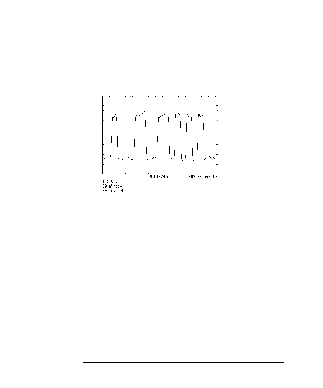
The display should look like the following figure.

2-27

Application Tutorials

Tutorial 8: Display the Data Pattern

Example Pattern Mode Display

Add Time Delay

6 Add time delay by pre ssing:

Setup, DELAY

Each push of the step keys (⇓ and⇑) gives a change in del a y equal to exactly one bit.

This technique c a n a lso be used to step the X o ffset of the mask one bit a t a time, to check for mask violations at each bit position.

7 Disconnect the RF cable from the patte rn g enerator’s TRIGGER OUT

connector and connect the cable to the CLOCK OUT connec tor.

Application Tutorials

T u to ria l 8: Displa y the Data Pattern

8 Set channel 2 by pressing:

CH2 is:, CLK OUT

Notice that the diagram sof tke y annotation no longer indicate s pattern mode, and a note is displayed on the screen as shown in the following figure.

Example Display of User-Error i n Pattern Mode

2-29

Application Tutorials

Tutorial 9: Constructing a Low-Pass Filter from a Transfer Function

This procedu re b u ilds a fourth order Bessel-Tho m son filter characterizing SONET/SDH transmitters operating at 2.48832 Gbit/sec. The filter is loaded into channel 1 user-correction data. The user-correction data is based on the transfer function:

----------------------------------------------------------------------------------- -=

p()

105 105y 45y

++++()

105

10y3y

where:

y 2.1140p=

jw wr⁄=

wr1.5πf

bit rate=

Note This tutorial of manually constructing a filter is useful as an example. To aid in

the construction of 4th order Bessel Thomson filters at other frequencies, use the MAKEFILT program located on the IBASIC UTILITIES FOR 71500 SERIES memory card. This card is supplied with the jitter and eye-diagram analyzer.

Construct the Filte r

For this example, f

=2.48832 Gbit/sec.

1 To construct the filter, press:

MENU, Config, TRACE POINTS and Enter 256

more 1 of 3, LINES DOTS LINES

2 Set an appropriate frequency ra ng e for the filter frequency poin ts b y se tting

the span to 2/f0. This is 803.75514 ps for this example. Press:

Main, SEC/DIV, and enter 803.75514 ps

Tutorial 9: Constructing a Low-Pass Filter from a Transfer Function

3 Turn the display off by pressing:

Application Tutorials

Traces, select:, TR1, display ON OFF OFF

4 Build the equation by pressing:

select:, TR2, input:, build eqn, CLR - END, SEL|EDT SEL

5 Turn the front-panel to hig hlight the j operand, and then pre ss:

INSERT

Continue using this technique to cons truct the trace equation shown in the following figure. Enter numbers using the front-panel num eric keypad.

2-31

Application Tutorials

Tutorial 9: Constructing a Low-Pass Filter from a Transfer Function

6 Build the trace equation shown in the following figure by pressing:

RETURN, select:, TR3, input:, build eqn, CLR - END, SEL|EDT SEL Build the trace equ a ti o n. Notice the cursor has wr apped to the following li ne . Be sure to include the last two right parenthesis char acte rs shown on the last line.

7 Turn auto-scaling on by pressing:

RETURN, format:, PHASE, Scale, AUTO-SCALE

8 Set the marker by pressing:

Markers, M1 ↓

Continue pressing M1 ( ↓) until TR3 is shown in the M1 ( ↓) softkey label.

9 Repeatedly press M2 ( ↓) until TR3 is shown in the M2 ( ↓) softkey label.

Application Tutorials

Tutorial 9: Constructing a Low-Pass Filter from a Transfer Function

10 Set the marker on 1.86224 GHz using the knob or numeric keypad.

11 Continue by pressing :

Scale, more 1 of 2, AUTO DELAY, Traces, store trace, to user correct , adaptiv ON|OFF ON

12 Store the filter resp onse in user-corr ections by pressing :

CHAN 1 USR COR

13 To view the response or to view the data, press:

Traces, select:, TR2, display ON|OFF OFF display ON|OFF OFF

, select:, TR1, input:

, select:, TR3,

2-33

Application Tutorials

Tutorial 9: Constructing a Low-Pass Filter from a Transfer Function

14 Highlight "UCORR1" using the knob.

15 Continue by pressing :

RETURN, Scale, AUTO-SCALE, page 1 of 2, Calib, user corr

Application Tutorials

Tutorial 9: Constructing a Low-Pass Filter from a Transfer Function

16 To store the filter to a memory card, press:

States, more 1 of 2, mass storage

17 If the mass-storage device needs to be selected, refer to “Saving to Mass

Storage” on page 3-34.

18 Save the user-corrections by pressing:

save, SAVE USR COR

19 To restore the instr um ent settings, press:

INSTR PRESET

2-35

Application Tutorials

Tutorial 10: Crea te a Vertical Histogr am

Tutorial 10: Create a Vertical Histogram

This tutorial creates a vertical histogram on data take n from a sine wave. The procedure, however, works for any type of waveform.

Select the Histogram Type

1 Display a trace to perform statistical analysis on. 2 Display the histogram menu by pressing:

page 1 of 2, Analyze, histogm

3 Select the trace to perform the statisti cal analy si s on by pre s si ng :

trace:

Use the knob to selec t the desired trace.

4 Select the Vertical Histogram function by pressing:

histog:, VERTICL HISTOGM VERTICL HISTOGM

Acquire the Data

5 Define the window for taking histogram data by pressing:

other, WINDOW MARKER1, WINDOW MARKER2

Notice the values of the marker positions are indicated at the top of the display.

Application Tutorials

Tutorial 10: Create a Vertical Hist ogram

6 Enter the number of samples to be taken for the histogram by pressing:

prev menu, NUMBER SAMPLES, # of samples, ENTER

The default number of sample s take n is 1000.

7 To draw the vertical histogram , pre ss:

SINGLE ACQUIRE

Data will be acquired once.

8 To continually acquire and update the his togram, press:

CONT ACQUIRE

2-37

Application Tutorials

Tutorial 10: Crea te a Vertical Histogr am

Perform Statistical Analysis

The range of sample points used to calculate the mean and standard deviation is the full screen.

9 To change the lim its , press:

other, UPPER LIMIT, LIMIT→ 0%-100%, new upper limit value, ENTER, LOWER LIMIT, LIMIT→ 0%-100%, new lower l imit value, ENTER

Notice the values of the limit-line positions are indicated at the top of the display.

Tutorial 10: Create a Vertical Hist ogram

10 To display a line indicating the location of the mean, pres s:

Application Tutorials

results, MEAN,

The mean and standard deviation values are also shown.

2-39

Application Tutorials

Tutorial 10: Crea te a Vertical Histogr am

11 To display a line indicating the location of the standard de viat ion , pres s:

STD DEV

Application Tutorials

Tutorial 11: Create a Horizontal Hist ogr am

Tutorial 11: Create a Horizontal Histogram

This tutorial creates a horizontal histogram on data taken from a sine wave. The procedure, however, works for any type of waveform.

Select the Histogram Type

1 Display a trace to perform statistical analysis on. 2 Display the histogram menu by pressing:

page 1 of 2, Analyze, histogm

3 Select the trace to perform the statisti cal analy si s on by pre s si ng :

trace:

Use the knob to selec t the desired trace.

4 Select the Vertical Histogram function by pressing:

histog:, HORZNTL HISTOGM

Acquire the Data

5 Define the window for taking histogram data by pressing:

other, WINDOW MARKER1, WINDOW MARKER2

Notice the values of the marker positions are indicated at the top of the display.

HORZNTL HISTOGM

2-41

Application Tutorials

Tutorial 11: Create a Horizontal Histo gram

6 Enter the number of samples to be taken for the histogram by pressing:

prev menu, NUMBER SAMPLES, # of samples, ENTER The default number of sample s take n is 1000.

7 To draw the horizontal histogram , pr ess:

SINGLE ACQUIRE

Data will be acquired once.

8 To continually acquire and update the histogram, press:

CONT ACQUIRE

Application Tutorials

Tutorial 11: Create a Horizontal Hist ogr am

Perform Statistical Analysis

The range of sample points used to calculate the mean and standard deviation is the full screen.

9 To change the lim its , press:

other, UPPER LIMIT, LIMIT→ 0%-100%, new upper limit value, ENTER, LOWER LIMIT, LIMIT→0%-100%, ne w lower limit value, ENTER

Notice the values of the limit-line positions are indicated at the top of the display.

2-43

Application Tutorials

Tutorial 11: Create a Horizontal Histo gram

10 To display a line indicating the locati o n of the mean, press:

results, MEAN

The mean and standard deviation values are also shown.

Application Tutorials

Tutorial 11: Create a Horizontal Hist ogr am

11 To display a line indicating the location of the standard de viat ion , pr es s:

STD DEV

2-45

Application Tutorials

Tutorial 11: Create a Horizontal Histo gram

Eye-Diagram Analyzer Reference

Eye-Diagram Analyzer Refer ence

Eye-Diagram Analyzer Reference

In this chapter, you will find information on the following topics:

• Performing Eye-Diagra m M easurement s 3-3

• Generating Histograms 3-7

• Masks and Limit Lines 3-9

• Eye-Diagram Menu Maps 3-12

• Agilent 70820A Menus 3-14

• Controlling the Display 3-16

• Calibrating the Eye-Diagram Analyzer 3-23

• Displaying Traces 3-25

• Using Markers 3-30

• Applying Mask T esting 3-31

• Saving to Mass Storage 3-34

• Creating Copies of the Display 3-47

• Agilent 70820A User-Corrections 3-49

• Agilent 70820A Calibration 3-61

Eye-Diagram Analyzer Reference

Performing Eye-Diagram Measurements

T o per form th e automat ic eye -diagra m measur ements, use the Measur e menu. With the exception of extinction rat io, these measurements must b e performed in eye mode.

Automatic Measurements

The Measure menu’s top two softkeys automatically start measurements:

• EXTINCT RATIO

• MEASURE EYE

• Use the EXTINCT RATI O softkey to automat ically compute the extinction rati o

in eye or eyel ine mode s. Thi s mea sur eme nt is a r at io of th e most p rev alent l ogical one level divided by the logical zero level over one bit interval. When making extinction ratio measurements in eyeline mode, the number of samples should be increased from the defaul t of 1000 to approximately 20000. This insures that a number of traces are evaluated to compute th e e xtinction ratio.

3-3

Eye-Diagram Analyzer Refer ence

Performing Eye-Diagram Measurements

Use the NUMBER SAM PLES softkey for this purpose.

• Use the MEASURE EYE to in itiate a number of automatic histogram me a su rements on an eye-diagram.

• Use the r/f tim ON OFF softkey to enable rise t ime an d fall time measur ements during the measure eye routine. This approximately doubles the measurement time.

• Use the UPPER THRSHLD and LOWER THRSHLD s oftkeys to set the upper

and lower edges for rise time and fall tim e measurements. These softkeys define the amplitude level to be used for the upper and lower part s of an edge definition fo r the a uto m a tic measurement func tions.

• The default upper threshold is 80%. The default lower threshold is 20%.

Measurement Definitions

Extinction Ratio This measurement is the ratio of th e m o st prevalent high le v el to the most

prevalent low level over one bit interval. The measurement results are displayed in both linear and logarithmic (10log) forms of the ra tio.

The peaks of the histogram are used to set initial limits for the computation of the one and zero leve ls. The i nitia l mean an d sigma o f the one level i s based on histogram data above the relative 50% point of the peaks. Th e l im its for the next evaluation of the histogram data are set to the initial mean plus-or-minus one sigma. The new mea n and sigma for the one level is determined. This process iterates several times until the sigma becomes small and the mean converges on the most prevalent one level. The determination of the most prevalent zer o level is based on the same algorithm , except the initial mean and sigma of the zero level are based on histogram data below the relative 50% point of the peaks.

1 Level (mean, σ) This measurement is the mean and sigma of the one level determined from a

20% window of a bit interval centered in the middle of the bit.

0 Level (mean, σ) This measurem ent is the mean and sigm a o f the zero level determined from a

20% window of a bit interval centered in the middle of the bit.

Eye Height This measurement is the difference between the mean minus-three sigma o f

the one level and the mean plus-three sigma of the zero level.

Eye-Diagram Analyzer Reference

Performing Eye-Diagram Measurements

Crossing Level This measurem ent is the amplitude th at the one level and zero le v el cross. It

also expresses the level as a percentage of the mean one le v el and mean zero level difference.

Eye Width Th is measurement is the eye width determined from the bit period and the

eye jitter. On the eye, the edges are defined to be the left crossing point plusthree sigma and the right crossing point minus-three sigma.

Eye Jitter (σ) This measurement is the sigma of a horizontal histogram at the crossing point.

Mean Rise Time This measurement is the mean time interval between a horizontal histogram

centered at the lower threshold point and a hori zontal histogram centered at the upper threshold point on a rising edge of an eye-diagram.

Mean Fall Tim e This measurement is the mean time interval between a horizontal histogram

centered at the upper threshold point and a horizontal hist og ram c ent ered at the lower threshold point on a fall ing edge of an eye-diagram.

Measure Fast Amplitude and Phase Transitions

The 70820A module measures fast ampl itu de and phase transitions on continuous wave (CW) and modulated signals. Time, frequency, and power sweeps can be performed from dc to 40 GHz. The 70820A module triggers on the RF input signal.

During stimulus/response measurements, the 70820A module controls an RF source instrument’s:

• frequency

• power

• pulse modulator

Viewing Repetitive and Non-Repetitive Signals

Because of the sampling techniques employed by the 70820A, the 70820A module is optimized for viewing repetitive input signals. However, there is single-shot operation for viewing baseband and modulated non-repetitive signals having bandwidths up to 10 MHz. Pre-trigger data can also be viewed. An example of using the single shot operation is measuring the turn-on characteristics of a pulse modulator. Single shot operation uses a maximum sampling rate of 20 MHz.

3-5

Eye-Diagram Analyzer Refer ence

Performing Eye-Diagram Measurements

For Optimum Performance

The 70820A module should be configured to:

• Control the RF source over the communications bus.

• Share the same frequency reference as the RF source.

Channels Versus Traces

The 70820A module has two input chann el s, four traces, and four trace memory registers.

• Channels are used to measure input signals.

• Traces are used to display measurement results.

• Trace memory registers can be used as a third channel.

Eye-Diagram Analyzer Reference

Generating Histograms

The 70820A can perform statistical analysi s on any displayed trace. After creating a vertical or horizontal histogram of the trace data, the display can show mean and standard deviation values of the histogram.

Histogram analysis is pe rformed using the Histogram menu. Press:

MENU, the left-s ide page 1 of 2, Analyze, Histogm The 70820A menus perform vertical or hori zontal histograms on any single

trace

You can control the number of samples taken, the window for valid data samples, and the sample bo unds for calculating mean and standard deviat ions

The Histogram Menu

3-7

Eye-Diagram Analyzer Refer ence

Generating Histogra m s

When generating histograms, yo u must perform the following basic steps:

1 Select a trace. 2 Select histogram typ e. 3 Enter the number of samples. 4 Set limits for acquired data. 5 Acquire the data. 6 Establish limit s for statistical a nalysis. 7 View the mean and standard de viation.

Histogram data can be acquired once using the SINGLE ACQUIRE softkey or continuously updated us ing the CONT ACQUIRE softkey .

Press other for this additional menu.

Eye-Diagram Analyzer Reference

Masks and Lim it Lin es

Masks and Limit Lines

Masks and limit lines allow you to test the shape (time or frequency versus amplitude) of a displayed response. Masks are closed polygon shapes. Limit lines are lines. Traces or measurement points that penetrate a mask or cross a limit line result in testing errors.

Two Masks Displayed on Screen

3-9

Eye-Diagram Analyzer Refer ence

Masks and Limit Lines

A Limit Line Displayed on Screen

Because you can perform repetitive testing of resp onse shapes, masks and limit lines are ideal for pass/fail testing on production lines. Y ou create, save, recall, and edit limit lines using the masks, limits menu. Access this menu using the left-side Analyze softkey.

Since masks and limit line s are treated similarly, in this chapter, most references to masks ap plies equally to limit lines.

Eye-Diagram Analyzer Reference

Masks and Lim it Lin es

Testing Responses

Once you’ve created a mask or limit line, set the following conditions for testing:

• Trace to which tes ting is applied.

• Violations defined as traces or m eas ure m ent points.

• Testing ends aft er a set number of errors.

• Testing ends aft er a set number of traces .

Use the test ON|OFF softkey to start testing. Testing stops whenever one of the following events occurs:

• A set number of trace sweeps.

• A set number of violations.

• test ON|OFF is se t to OF F .

Numbers displ a yed at the bottom of the screen indicate t he number of violations and trace sweeps that have occurred. The fol lowing figure shows a response that ha s v iolated a limit lin e three times on three sw e eps.

3-11

Eye-Diagram Analyzer Refer ence

Eye-Diagram Menu Maps

The two menu maps in this section graphically represent the eye-diagram analyzer’s softkey menus.

Setup and Trg, Cal Menus

Eye-Diagram Analyzer Reference

Eye-Diagram Menu Maps

Traces, Measure, Markers, Masks, and Mass Storage Menus

3-13

Eye-Diagram Analyzer Refer ence

Agilent 70820A Menus

This section discusses the softkey menus for the 70820A microwave transition analyzer module. To learn about the eye-diagram analyzer’s menus, refer to

“Eye-Diagram Menu Maps” on page 3-12. These menus provide additional fea-

tures useful for running the eye-diagram analyzer. You will find the preview feature discussed in this chapter very useful. It dis-

plays the programming command, corresponding to the response received, when most softkeys are pr essed.

Most front-panel controls are accessed via softkey menus . So ftke y s are the seven buttons located on each side of the screen. The functio ns of softkeys change according to the menus display ed on the scre en .

Page 1 of Top Level Menus

Eye-Diagram Analyzer Reference

Agilent 70820A Menus

The Left-Side Softkeys

Use the softkeys located on the left side of the display to access the twelve major menus. These softkeys are shown in two pages. Press page 1 of 2 to view

the second page of softkeys. When the 70820A module first turns on, the Main menu is automatically selected.

Page 2 of Top Level Menus

3-15

Eye-Diagram Analyzer Refer ence

Controlling the Display

To Control the Number of Bits Displayed

To Measure in Optical Power Units

The Setup menu’s BIT INTVL softkey allows you to select the number of bits that will be displayed on the screen. The horizontal time scale automatically changes to the appropriate setting. Use DELAY to enter time delay. The amount of delay is entered in bits. Use this feature, in pattern mode, to view different portions of the PRBS waveform.

The amount of delay can be as much as 1000 times the time span. In addition, the eye-diagram analyzer can v iew the trac e before t he tr igger ev ent. Negati ve time delay up to {-time span}over2 can be entered.

Set the number of bits displayed by pressing:

Setup, BIT INTVL and enter the number of bits to display.

Set the time delay by pr essing:

Setup, DELAY and enter the desired time delay

The Trg, Cal menu’s CH1 EX T ATTEN and CH2 EXT ATTEN softkeys all ow you to specify any external attenuation or optical-to -el ectrical responsivity conversion between the source and input channels. Specifying an attenuation on channel 1 changes the measurement plane from the front -panel channel 1 connector to include the indicated attenuati on. Specifying an optical-to-electrical responsivity displays optical units referenced to the input of the opticalto-electrical converter. Channel and marker readouts change to watts/div. Also, the CH1 EXT ATTEN softkey changes to read CH1 RSPVTY (responsivity).

To measure the optical power, press:

Trg, Cal, CH1 EXT ATTEN and enter the responsivity value in watt s/d iv

Notice the CH1 EXT ATTEN softkey changes to read CH1 RSPVTY (responsivity).

Eye-Diagram Analyzer Reference

Controlling the Display

To Improve the Sensitivity in Eyeline Mode

To Extend the Bandwidth to 40 GHz

In eyeline mode, additional eye filtering can be applied to improve the measurement sensitivity. This can be an advantage when measuring extinction ratios on low-level signals. Use the eyefltr ON OFF softkey to apply the filter. When the pattern repetition frequency is greater than 10 MHz, internal filtering is applied tha t p rov ides a 20 dB signal-t o-noise improvement. For pattern repetition freque nc i es less than 10 MHz, softw are filtering is applied that allows variable signal-to-noise improvement versus sweep time.

To improve sensitivity, press:

Setup, diagram, EYELINE or PATTERN, eyefltr ON OFF ON

Use the front-panel knob to adjust the amount of filtering applied.

Use the extd BW ON OFF softkey to enable RF corrections which extend the measurement bandwidth of the eye-diagram analyzer to 40 GHz. Extended bandwidth operation can be us ed in both eyeline and pattern modes, but not in eye mode.

1 Extend the measurement bandwidth by pressing:

Setup, diagram, EYELINE or PATTERN

The extended 40 GH z ba ndwidth cannot be us ed in eye mode.

2 Turn the extended bandwidth on by pressing:

Trg, Cal, more 1 of 2,, extd BW ON|OFF ON

To Apply UserCorrections

User-corrections provide a convenient method for modifying the display of input signals. Some of the applications for user-corrections include the following:

• Filtering inpu t signals to simulate the effects of circ uit design.

• Compensating fo r frequency and phase response of external probes.

• Compensating for fr equency and phase response of externa l test setups.

• Compensating for the frequency response of optical to electrical converters.

Several Bessel-Thomson software filters are included on the 70874A eye-diagram analyzer’s memory card. These filters can be applied as user-corrections in the eyeline and pattern modes. (User corrections must be off in eye mode.) User correction files are identified by the prefix a_ as shown in the following table. The files AUTOST and 70874 comprise the eye-diagram analyzer program.

3-17

Eye-Diagram Analyzer Refer ence

Controlling the Display

To learn more about these files and about cre ating and applying user-corrections, refer to “Tutorial 5: Use Software Filters” on page 2-15.

User-Correct ion Files

File Name File Data

a_bt248832 4th order Bessel- Thomson filter f or 2.48832 Gbit/sec transmission. a_bt_62208 4th order Bessel- Thomson filter for 622.08 Mbit/sec transmission. a_bt_15552 4th order Bessel- Thomson filter for 155.52 Mbit/sec transmission.

1 Place the 70874A eye-diagram analyzer memory card in the front-panel card

slot. The 70874A eye-diagram analyzer must already be loade d int o mem or y.

2 Display the eye-diagram analyzer’s menus by pressing:

USER, Setup, diagram, EYELINE or PATTERN

User corrections can not be applied in eye mode.

3 Display a catalog of the files contained on the memory card by pressing:

Mass Storage

Rotate the front-panel knob to highlight the desired file. User correction files are identified by the prefix a_.

4 Load the file by pressing:

LOAD FILE

Eye-Diagram Analyzer Reference

Controlling the Display

The file is loaded when user-corrections loaded is displayed on the screen.

5 Turn the user correction function on by pressing:

Trg, Cal, more 1 of 2, usr cor ON|OFF ON

3-19

Eye-Diagram Analyzer Refer ence

Controlling the Display

User-Corrections Applied to the Data

To View 70820A Menus

To Return to the Jitter Analyzer (or Eye-Diagram Analyzer)

To Preview Programming Commands

To View the Firmware Date Code

Press MENU.

Press USER. If the eye-diagram analyzer’s menus are not displayed, load the program as

explained in Chapter 1, “Getting Started”.

Press MENU, Config, more 1 of 3, preview ON|OFF ON For a demonstration of the Preview function, press persist ON|OFF. Notice the

corresponding programming command DISP:PERS 1024 is displayed at the bottom of the scr een.

Press MENU, Config, more 1 of 3, more 2 of 3, system, ROM VERSION

Agilent Technologies 71501D User Manual

Specifications and Main Features

Frequently Asked Questions

User Manual

Contents

Getting Started

Steps for Setting Up Eye-Diagram Analysis

Application Tutorials

Tutorial 1: Measure Eye-Parameters

Tutorial 2: Measure in Optical Power Units

Tutorial 3: Meas ur e Extinction Ratios on Low-Level Si gnals

Tutorial 4: Measure Laser Turn-on Delay

Tutorial 5: Use Software Filters

Tutorial 6: Test to Industry Standards

Tutorial 7: Default and Custom Mask or Limit Line Testing

T u to ria l 8: Displa y the Data Pattern

Tutorial 9: Constructing a Low-Pass Filter from a Transfer Function

Tutorial 10: Crea te a Vertical Histogr am

Tutorial 11: Create a Horizontal Hist ogr am

Eye-Diagram Analyzer Reference

Performing Eye-Diagram Measurements

Generating Histograms

Masks and Lim it Lin es

Eye-Diagram Menu Maps

Agilent 70820A Menus

Controlling the Display