YOKOGAWA LL1200 Operation Manual

Download

Instruction

Model LL1200

Manual

PC-based Custom Computation Building Tool

IM 5G1A11-01E

2nd Edition

Introduction

This instruction manual describes the functions of Model LL1200 PC-based Custom Computation Building Tool (hereinafter, simply referred to as the LL1200 tool in the main text), which is used with Model US1000 Digital Indicating Controller (hereinafter, simply referred to as the US1000 controller in the main text), and how to operate the tool.

The LL1200 tool consists of the following component tools.

• Custom computation building tool

• Parameters setting tool

This manual focuses exclusively on the custom computation building tool. For details on the handling of the parameters setting tool, see the Model LL1100 PC-based Parameters Setting Tool instruction manual (IM 5G1A01-01E).

■ Intended Readers

This manual is intended for people familiar with the functions of the US1000 digital indicating controller and capable of working with Windows 95 or Windows NT 4.0, such as instrumentation and control engineers and personnel in charge of maintaining instrumentation and control equipment.

■ Related Documents

The following instruction manuals all relate to the LL1200 tool. Read them as necessary. The codes enclosed in parentheses are the document numbers.

• US1000 Digital Indicating Controller-Operation (IM 5D1A01-01E)

• US1000 Digital Indicating Controller-Functions (IM 5D1A01-02E)

• US1000 Digital Indicating Controller-Communication Functions (IM 5D1A01-10E)

• LL1100 PC-based Parameters Setting Tool (IM 5G1A01-01E)

• LL1200 PC-based Custom Computation Building Tool-User’s Reference (IM 5G1A11-02E)

■ Trademarks

Windows 95 and Windows NT 4.0 are registered trademarks of Microsoft Corporation, USA.

Supplied with the US1000 controller, this manual explains the basic operations of the controller.

Supplied with the US1000 controller, this manual explains the functions of the controller in detail.

An instruction manual for the communication function of the US1000 controller. Supplied with models having the optional communication function.

An instruction manual for setting the parameters of the US1000 controller from a personal computer. Supplied with the LL1100 PC-Based Parameters Setting Tool or the LL1200 PC-based Custom Computation Building Tool.

An instruction manual that describes the functions needed to create US1000 custom computations. Refer to this manual if you are not familiar with the types of functions available or how these functions work. Supplied with the LL1200 PC-based Custom Computation Building Tool.

IM 5G1A11-01E

Visual Inspection and Cross-check of Accessories

Visually inspect the purchased product upon delivery to make sure it is not damaged in any way. Store the box and inner packing material of the package in a safe location - they may be needed should the product fail and need to be sent back to the manufacturer for repair.

■ Cross-check of Model and Suffix Codes

Refer to the following table to make sure the model and suffix codes of the LL1200 tool are as specified in your order.

Model Code Description

LL1200

Suffix Code

-E10

Custom computation building tool* Model for use with IBM PC/AT-compatible personal computers

* The LL1200 tool includes the same parameter setting function as the LL1100 PC-based Parameters

Setting Tool.

■ Confirmation of the Model and Suffix Codes

Make sure the delivered package contains all of the following items. If any item is missing or found to be damaged, immediately contact the sales office or dealership from which you purchased the product.

• 3.5-in. floppy disks (5 disks)

• Dedicated adapter, supplied with two AAA-size batteries (one unit)

• Dedicated cable (one cable)

• Model LL1100 PC-based Parameters Setting Tool instruction manual (one copy)

• Model LL1200 PC-based Custom Computation Building Tool instruction manual (one copy)-This manual

• Model LL1200 PC-based Custom Computation Building Tool -User’s Reference manual (one copy)

IM 5G1A11-01E

Documentation Conventions

■ Notational Conventions in This Manual

This manual uses the following notational conventions.

[ ]: indicates the name of a dialog box or message, or a view name (name indicated in the upper-left corner of a dialog box.) Example: • The [Input Block] dialog box appears.

< >: indicates the name of a command in a dialog box or the name of a tool menu (or a command in the menu). Examples: • Click the <OK> button.

• Click the <Cancel> button.

• Click the <Input Block> button.

• From the tool menus, choose <File>, then <Open>.

“ ”: indicates the text typed. Example: • Type “ABCD” in the <xxx> text box.

NOTE

Draws attention to information that is essential for understanding the operation and/or features of the product.

TIP

Gives additional information to complement the present topic and/or describe terms used in this document.

See Also

Gives reference locations for further information on the topic.

■ Description of Displays

(1) Some of the representations of product displays shown in this manual may be exaggerated,

simplified, or partially omitted for reasons of convenience when explaining them.

(2) Figures and illustrations representing the controller’s displays may differ from the real displays in

regard to the position and/or indicated characters (upper-case or lower-case, for example), to the extent that they do not impair a correct understanding of the functions and the proper operation and monitoring of the system.

IM 5G1A11-01E

iii

Notices

■ Regarding This Instruction Manual

(1) This manual should be passed on to the end user. Keep at least one extra copy of the manual in a

safe place.

(2) Read this manual carefully to gain a thorough understanding of how to operate this product before

you start using it.

(3) This manual is intended to describe the functions of this product. Yokogawa M&C Corporation

(hereinafter simply referred to as Yokogawa M&C) does not guarantee that these functions are suited to the particular purpose of the user.

(4) Under absolutely no circumstance may the contents of this manual, in part or in whole, be tran-

scribed or copied without permission. (5) The contents of this manual are subject to change without prior notice. (6) Every effort has been made to ensure accuracy in the preparation of this manual. Should any

errors or omissions come to your attention however, please contact your nearest Yokogawa

representative or our sales office.

■ Regarding Protection, Safety, and Prohibition Against Unauthorized Modification

(1) In order to protect the product and the system controlled by it against damage and ensure its safe

use, make sure that all of the instructions and precautions relating to safety contained in this

document are strictly adhered to. Yokogawa does not guarantee safety if products are not handled

according to these instructions. (2) The following safety symbols are used on the product and/or in this manual.

●Symbols Used on the Product and in This Manual

CAUTION

This symbol on the product indicates that the operator must refer to an explanation in the instruction manual to avoid the risk of injury or death of personnel or damage to the instrument. The manual describes how the operator should exercise special care to avoid electrical shock or other dangers that may result in injury or loss of life.

Protective Grounding Terminal This symbol indicates that the terminal must be connected to ground prior to operating the equipment.

Functional Grounding Terminal This symbol indicates that the terminal must be connected to ground prior to operating the equipment.

IM 5G1A11-01E

●Symbol Used in This Manual Only

Indicates that operating the hardware or software in this manner may damage it or lead to system failure.

■ Force Majeure

(1) Yokogawa M&C does not make any warranties regarding the product except those mentioned in

the WARRANTY provided separately. (2) Yokogawa M&C assumes no liability to any party for any loss or damage, direct or indirect,

caused by the use or any unpredictable defect of the product. (3) Be sure to use the spare parts approved by Yokogawa M&C when replacing parts or consumables. (4) Modification of the product is strictly prohibited. (5) This software may be used with one specified computer only. You must purchase another copy of

the software for use on each additional computer. (6) Copying this software for purposes other than backup is strictly prohibited. (7) Store the floppy disk(s) (original medium or media) containing this software in a secure place. (8) Reverse engineering such as the disassembly or decompilation of software is strictly prohibited. (9) No portion of the software supplied by Yokogawa M&C may be transferred, exchanged, leased or

sublet for use by any third party without the prior permission of Yokogawa M&C.

WARNING

IM 5G1A11-01E

Introduction........................................................................................................................... i

Visual Inspection and Cross-check of Accessories ........................................................... ii

Documentation Conventions.............................................................................................. iii

Notices .................................................................................................................................. iv

Contents ............................................................................................................................... vi

1. Overview ..................................................................................................................... 1-1

1.1 Function Overview of the LL1200 Tool ........................................................ 1-1

1.2 Operating Environment of the LL1200 Tool and Wiring Specifications ...... 1-4

1.3 Model and Suffix Codes of Applicable US1000 Controller Models............. 1-6

2. Setup ....................................................................................................................... 2-1

2.1 Installing the LL1200 Tool ............................................................................. 2-1

2.2 Uninstalling the LL1200 Tool ........................................................................ 2-4

2.3 Connecting the US1000 Controller to the Personal Computer ...................... 2-5

3. Using the LL1200 Tool .............................................................................................. 3-1

3.1 Starting and Exiting the Tool .......................................................................... 3-1

3.1.1 Starting the Tool....................................................................................... 3-1

3.1.2 Exiting the Tool ....................................................................................... 3-2

3.2 Flow of Working with the LL1200 Tool........................................................ 3-3

3.3 Dialog Boxes and Tool Menus ....................................................................... 3-4

4. Basic Operations for Configuring Custom Computations

and Relevant Explanations ....................................................................................... 4-1

4.1 Step 1: Choosing the Way Computations Are Configured ............................ 4-2

4.2 Step 2: Configuring Custom Computations in an Input Block ...................... 4-8

4.2.1 Step 2-1: Registering Computation Modules .......................................... 4-9

4.2.2 Step 2-2: Configuring the Inputs and Parameters

of Computation Modules ....................................................................... 4-13

4.2.3 Step 2-3: Connecting Computation Modules to the Control

and Computing Section.......................................................................... 4-17

4.2.4 Step 2-4: Setting the Analog-input Burnout Function ........................... 4-22

4.3 Step 3: Configuring Custom Computations in an Output Block ................. 4-23

4.3.1 Step 3-1: Registering Computation Modules ........................................ 4-24

4.3.2 Step 3-2: Configuring the Inputs and Parameters

of Computation Modules ....................................................................... 4-28

4.3.3 Step 3-3: Connecting Computation Modules to Output Signals ........... 4-32

4.4 Step 4: Configuring the Parameters of Ten-segment Linearizers

3 and 4 (as necessary) ................................................................................... 4-36

4.5 Step 5: Configuring USER Parameters (as necessary) ................................ 4-38

IM 5G1A11-01E

5. Basic Operations for Configuring Custom Displays

and Relevant Explanations ....................................................................................... 5-1

5.1 Step 1: Choosing the Method of Custom Display Configuration .................. 5-2

5.2 Step 2: Configuring Custom Displays ............................................................ 5-8

5.2.1 Step 2-1: Choosing the Custom Display.................................................. 5-9

5.2.2 Step 2-2: Setting Conditions Needed to Switch to Custom Displays.... 5-14

5.3 Step 3: Defining the Security Function (as necessary) ................................ 5-16

6. Editing .......................................................................................................................6-1

6.1 Editing Custom Computations ........................................................................ 6-1

6.1.1 Moving Computation Modules................................................................ 6-1

6.1.2 Deleting Computation Modules............................................................... 6-3

6.1.3 Adding Computation Modules ................................................................ 6-4

6.1.4 Changing the Order in Which Computation Modules Run ..................... 6-4

6.1.5 Changing the Way Computation Modules Are Connected ...................... 6-6

6.2 Editing Custom Displays .............................................................................. 6-13

6.2.1 Deleting Custom Displays ..................................................................... 6-13

6.2.2 Adding Custom Displays....................................................................... 6-14

7. Working with Custom Computation and Custom Display Data Files ................ 7-1

7.1 Setting the File Information ............................................................................ 7-1

7.2 Setting Comments for I/O Signals.................................................................. 7-2

7.3 Reading/Saving Data from/on Disk and Comparing Data Values................. 7-3

7.3.1 Reading Data from Disk .......................................................................... 7-3

7.3.2 Saving Data on Disk ................................................................................ 7-5

7.3.3 Compare between Data Values ................................................................ 7-5

8. Uploading/Downloading Data from/to US1000 Controller

and Comparing between Data Values ..................................................................... 8-1

8.1 Uploading Data from US1000 Controller ...................................................... 8-1

8.2 Downloading Data to US1000 Controller ...................................................... 8-3

8.3 Comparing Data Values with Those of the US1000 Controller .................... 8-5

9. Printing Custom Computations................................................................................ 9-1

10. Configuring Parameters ..........................................................................................10-1

11. Custom Computation Monitor ............................................................................... 11-1

11.1 Preparations for Monitoring of Custom Computations ................................ 11-2

11.2 Monitoring Custom Computations Configured in an Input Block .............. 11-2

11.2.1 Monitoring Data Values Fed to/from an Input Block ............................ 11-3

11.2.2 Monitoring the Inputs and Parameters of Computation Modules ......... 11-5

11.3 Monitoring Custom Computations Configured in an Output Block............ 11-6

11.3.1 Monitoring Data Values Fed to/from an Output Block.......................... 11-6

11.3.2 Monitoring the Inputs and Parameters of Computation Modules ......... 11-8

IM 5G1A11-01E

vii

12. Examples of Custom Computation and Custom Display Configurations .........12-1

12.1 Example 1: Applying Corrective Computation to the PV Input.................. 12-3

12.2 Example 2: Showing the PV Input Value

before Corrective Computation................................................................... 12-16

12.3 Example 3: Implementing Simple Logic Operations ................................. 12-25

12.4 Example 4: Applying Temperature-based Flowrate Corrections to

the PV Input ................................................................................................ 12-34

12.5 Example 5: Configuring Timers ................................................................. 12-44

12.5.1 Configuring a Four-second Timer........................................................ 12-44

12.5.2 Configuring a Fixed-interval Five-second Timer................................. 12-55

12.6 Example 6: Setting Parameters ................................................................... 12-62

12.7 Example 7: OR Function of Alarm Outputs .............................................. 12-69

13. Maintenance and Troubleshooting ......................................................................... 13-1

13.1 Replacing the Batteries ................................................................................. 13-1

13.2 Troubleshooting Problems with the Display

and Communication Functions ..................................................................... 13-3

13.2.1 Problems with the Display Functions .................................................... 13-3

13.2.2 Problems with the Communication Functions....................................... 13-3

Appendix 1. WORKSHEET ....................................................................................... A1-1

Appendix 2. DATASHEET ......................................................................................... A2-1

Appendix 3. Restrictions Imposed Depending on the Suffix Code

and/or Controller Type ......................................................................... A3-1

Appendix 4. Areas for Storing Data Output from Computation Modules ........... A4-1

Revision Record

viii

IM 5G1A11-01E

Chapter 1 Overview

1. Overview

This chapter first explains what custom computation is and then introduces the tool used to configure these computations and the model and suffix codes of the US1000 controller models to which the tool applies. This chapter also discusses the system requirements that must be met to be able to use the LL1200 tool and shows external views of the dedicated adapter and cable.

1.1 Function Overview of the LL1200 Tool

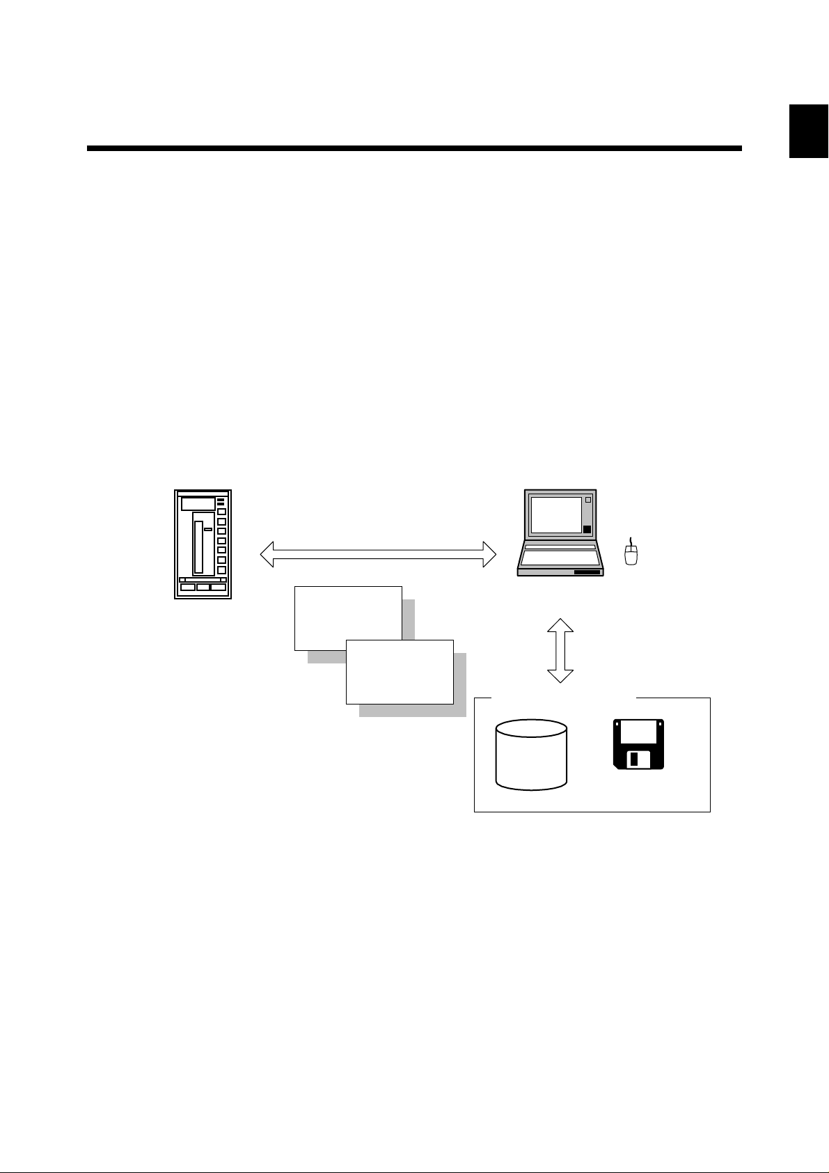
The LL1200 tool is designed to run on a personal computer connected to the US1000 controller. You can set a variety of functions for the US1000 controller from the personal computer. Inversely, you can read the settings from the US1000 controller. In addition to these operations, you can set the various parameters of the US1000. This particular function is the same as the one offered by Model LL1100 PC-based Parameters Setting Tool, another tool used with the US1000 controller. This manual does not therefore discuss this function in particular. When you use this function in your practical applications, refer to the Model LL1100 PC-based Parameters Setting Tool instruction manual (supplied together with this manual).

Uploading from/downloading

to US1000 controller

US1000 controller

(One-to-one communication)

Notebook PC

Custom computations

Custom displays

Saving to/reading from disks

Hard disk

Mouse

Reading from/saving

to disks

Floppy disk

Figure 1.1.1 Conceptual View of LL1200 Tool

The LL1200 tool is designed to run under Windows 95 or Windows NT 4.0. For details on how to use the personal computer and Windows software, see their respective instruction manuals.

IM 5G1A11-01E 1-1

The US1000 controller comes with built-in control functions and various controller modes (US modes) that provide different I/O computing functions. These modes are designed to support their

respective control applications. From these choices, you can choose one that best meets your application needs. In some control applications, however, you may want to execute special computations based upon specific input data or have a contact output of a specific data item in a specific control sequence. To be able to meet these needs, the US1000 controller provides a separate controller mode with which you can freely program your own computations. Computing functions available in these modes are referred to as custom computations.

Custom computations allow you to perform a variety of calculations based on input and output signals. These calculations include not only the four arithmetic operations and logical operations but also tensegment linear approximations, temperature and humidity computations, temperature-based correction coefficient computations, pressure-based correction coefficient computations, and so on. For example, you can use the four arithmetic operations to apply the desired type of correction to input signals, or use a logical operation to program a sequencing process that works between input and output contacts.

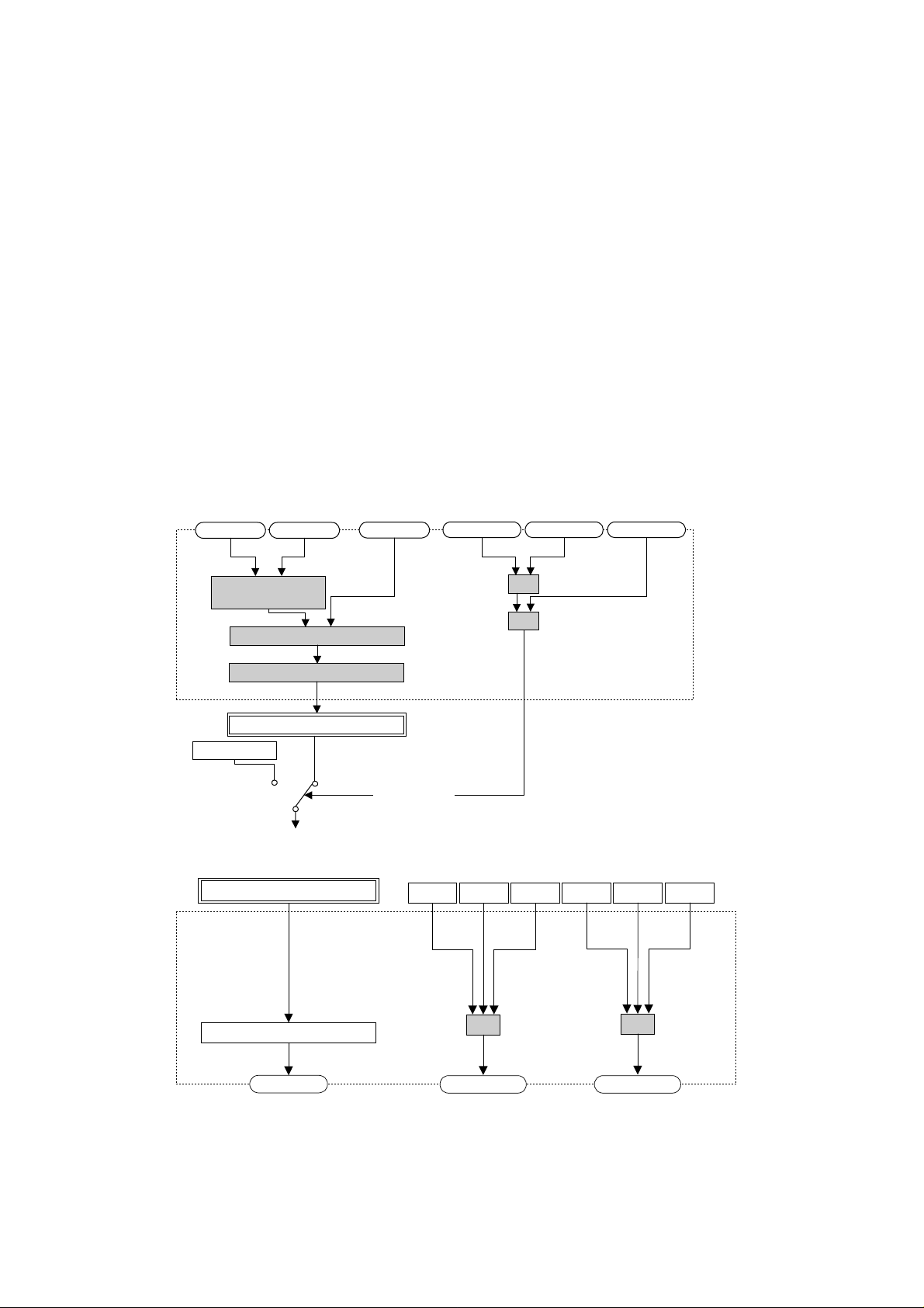
Custom computations are configured using the given methods of block connection, as shown in Figures 1.1.2 and 1.1.3.

Flowrate

Temperature-based

flowrate correction

MV output

Temperature

Fluid pressure correction

Square-root computation

Control and computing section

Pressure

A/M switching

Contact input 1

Contact input 2 Contact input 3

AND

Figure 1.1.2 Custom Computations Applied to Input Signals

Control and computing section

Alarm 1

Alarm 2 Alarm 3 Alarm 4 Alarm 5 Alarm 6

1-2

Control output processing

MV output

Contact output 1

Contact output 2

Figure 1.1.3 Custom Computations Applied to Output Signals

IM 5G1A11-01E

Chapter 1 Overview

When custom computations are in use, you can also freely configure the operation displays of the US1000 controller to suit your desired view. This function is designed so that you can choose from the preset menus the types of data items, the sequence in which the data items are shown, and the conditions required to show them on the PV and SV digital displays of the US1000 controller. The displays thus configured are referred to as custom displays.

Normally, the term “custom computing function” is used to include both the custom computation and custom display functions.

IM 5G1A11-01E 1-3

1.2 Operating Environment of the LL1200 Tool and Wiring Specifications

■ System Requirements

●Personal computer: Windows 95- or Windows NT 4.0-enabled IBM PC/AT-compatible model

●Operating system: Windows 95 or Windows NT 4.0

●CPU: 90-MHz Pentium processor or superior is recommended.

●Main memory: 16 MB minimum for Windows 95 or 24 MB minimum for Windows NT 4.0 is

recommended.

●Hard disk

Memory space required to store the tool’s programs: 9 MB Memory space required to store the parameter data: 2 MB minimum

●CRT display

800 3 600 pixels or superior Should be capable of handling at least 256 colors. Smaller fonts should be used.

●RS-232C communication ports: One channel, with 9-pin D-Sub connector

●3.5-inch floppy drive: One drive.

●Printer: As necessary.

■ Dedicated Adapter

●Communication method

US1000: Optical, contactless, bidirectional serial communication Personal computer: RS-232C half-duplex communication using the dedicated cable

●Power supply: Two AAA-size batteries or external power source

Use of an external power source is recommended for tuning over a prolonged time period.

●Battery life: Approximately 50 hours (when the adapter is continuously operated on alkaline

batteries)

●Specifications of external power source

●Should comply with EIAJ RC-6705.

Input ratings: 5 V DC/50 mA (Purchase a commercially available plug and AC adapter for the external power source.)

●Ambient temperature range: 0 to 50˚C

●Ambient humidity range: 20 to 90%RH (non-condensing)

●Transport and storage conditions: -25 to 70˚C, 5 to 95%RH (non-condensing)

●Dust- and water-proof construction: Not applied.

●Standards: Complies with the CE Mark system (EMC standard only)

1-4

WARNING

The dedicated adapter is not waterproof. Do not use the adapter in locations that are likely to be exposed to splashes of water or other liquids.

IM 5G1A11-01E

Chapter 1 Overview

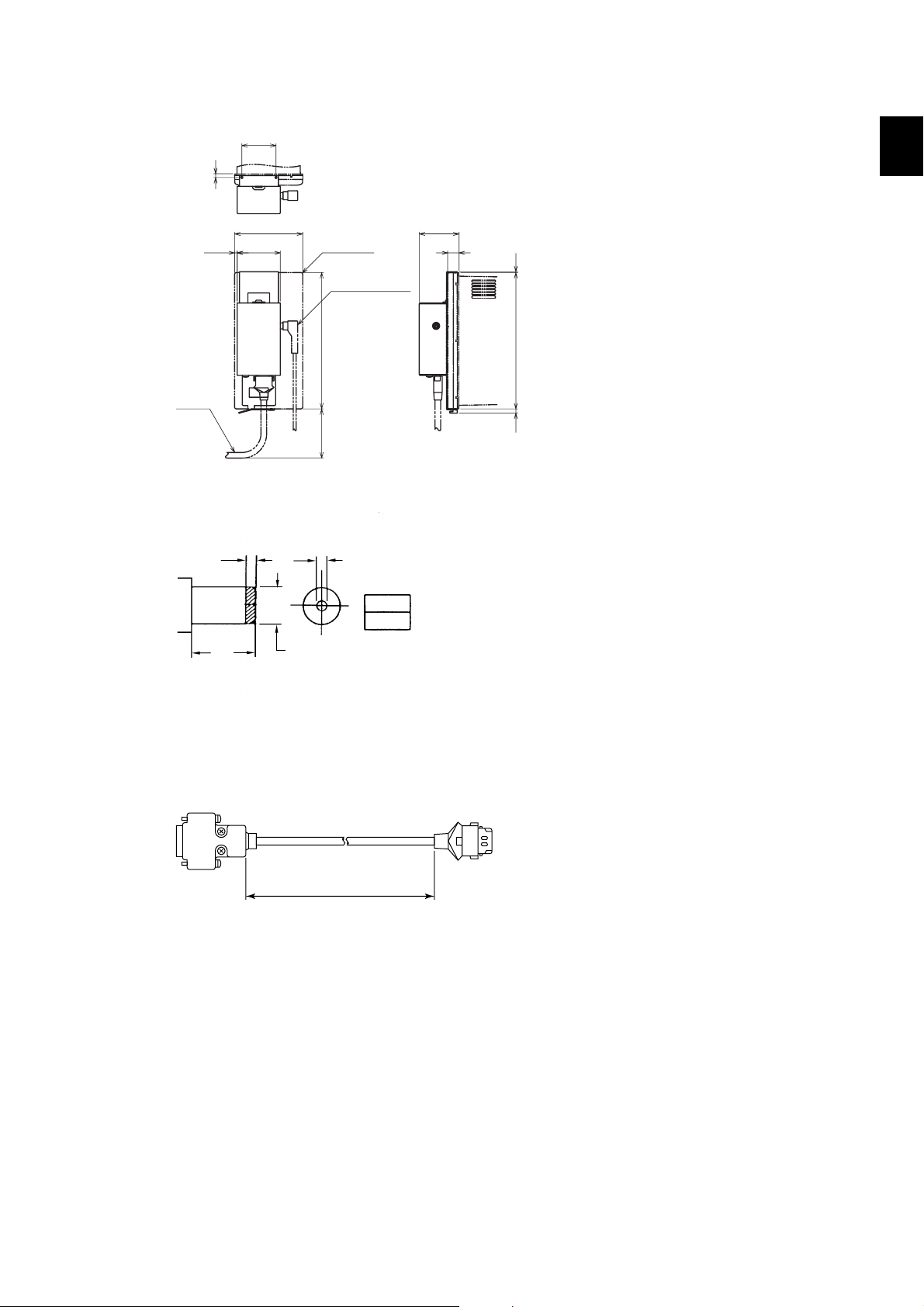
36 (1.42)

42 (1.66)

12 (0.47)

0.8

(0.03)

144 (5.69)

4.5 (0.18)

CABLE

2.8

(0.11)

72 (2.85)

45.5 (1.80)

US1000

DC POWER PLUG

144

(5.69)

(2.06)

Figure 1.2.1 External View of the Dedicated Adapter

Mate Plug

1.5

(0.06)

unit: mm

D' DIA

unit : mm(inch)

(0.37)

Figure 1.2.2 External View of the External Power Inlet on the Dedicated Adapter

■ Dedicated Cable

Cable with 9-pin D-Sub connector for IBM PC/AT-compatible models: 3-m long

To PC

Figure 1.2.3 External View of the Dedicated Cable

9.5

D' DIA

2.1

5.5 DIA

(0.08)

(0.22)

(EIAJ)

About 3000 (118.1)

PC/AT compatible machine

unit : mm(inch)

To adapter

IM 5G1A11-01E 1-5

1.3 Model and Suffix Codes of Applicable US1000 Controller Models

The US1000 controller models allowing for custom computations are as follows.

Model and Suffix Code Combination Description

US1000-11 US1000-11/A10 US1000-21 US1000-21/A10

When using custom computations for any of these controller models, set the controller mode (US mode) to “21.”

See Also

“What are the Controller Modes (US Modes)?” in Chapter 2, “Controller Modes (US Modes)” of the US1000 Digital Indicating Controller-Functions instruction manual (IM 5D1A01-02E).

Enhanced model of digital indicating controller without communication function Enhanced model of digital indicating controller with communication function Position-proportional model of digital indicating controller without communication function Position-proportional model of digital indicating controller with communication function

1-6

IM 5G1A11-01E

2. Setup

This chapter explains how to set up the hardware and software necessary to work with the LL1200 tool.

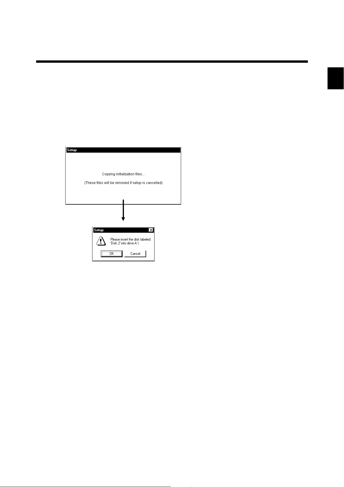
2.1 Installing the LL1200 Tool

(1) Insert Disk 1 of the LL1200 tool into the floppy drive. (2) From the Start menu of Windows, choose <Run . . .>. Type the name of the floppy drive

as \Setup.exe and click the <OK> button.

(3) To continue, follow the instructions given in each dialog box.

Chapter 2 Setup

Figure 2.1.1 Window for Installation Operations

When installation is complete, the <LL1200> option is registered with the <Programs> command in the <Start> menu.

IM 5G1A11-01E 2-1

■ LL1200 File Package and Files of Information on Configured Custom Computations

The LL1200 package files comprise a set of the files that are needed to run the LL1200 tool, the installation program, sample files, help files, and so on.

NOTE

The file names should contain no more than 16 half-byte alphanumeric characters, and their extensions should be as shown in the following tables.

●LL1200 Package Files

When the installation of the LL1200 tool is complete, the folders in the following table are set up.

Folder Name File

US Package files (those other than the sample files)

US\SAMPLE Sample files (********.1sc) US\USER User files (********.1sc, ********.1ec, ********.1sp, ********.1ep and ********.csv)

●Sample Files

The sample files contain information on custom computations in the I/O blocks of controller modes (US modes) 1 to 15.

Sample File File Name

Controller mode (US mode) 1: Sample file for single-loop control USM01.1SC Controller mode (US mode) 2: Sample file for cascade primary-loop control USM02.1SC Controller mode (US mode) 3: Sample file for cascade secondary-loop control USM03.1SC Controller mode (US mode) 4: Sample file for cascade control USM04.1SC Controller mode (US mode) 5: Sample file for loop control for backup USM05.1SC Controller mode (US mode) 6: Sample file for loop control with PV switching USM06.1SC Controller mode (US mode) 7: Sample file for loop control with PV auto-selector USM07.1SC Controller mode (US mode) 8: Sample file for loop control with PV-hold function USM08.1SC Controller mode (US mode) 11: Sample file for dual-loop control USM11.1SC Controller mode (US mode) 12: Sample file for temperature and humidity control USM12.1SC Controller mode (US mode) 13: Sample file for cascade control with two universal inputs USM13.1SC Controller mode (US mode) 14: Sample file for loop control with PV switching and two universal inputs USM14.1SC Controller mode (US mode) 15: Sample file for loop control with PV auto-selector and two universal inputs USM15.1SC

2-2

●User Files

The user files contain information on user-created custom computations.

Type of User File File Name

Data file for custom computations and displays ********.1sc Results of comparison between custom-computation data (text file) ********.1ec Parameter data file ********.1sp Results of comparison between parameter data (text file) ********.1ep Data for printouts (CSV-format file) ********.csv

IM 5G1A11-01E

●Help Files

Type of Help File File Name

Parameters setting tool help PARA.hlp Custom computation building tool help CUST.hlp Description of D-registers and I-relays DREG.hlp Description of module information MODUL.hlp

Chapter 2 Setup

IM 5G1A11-01E 2-3

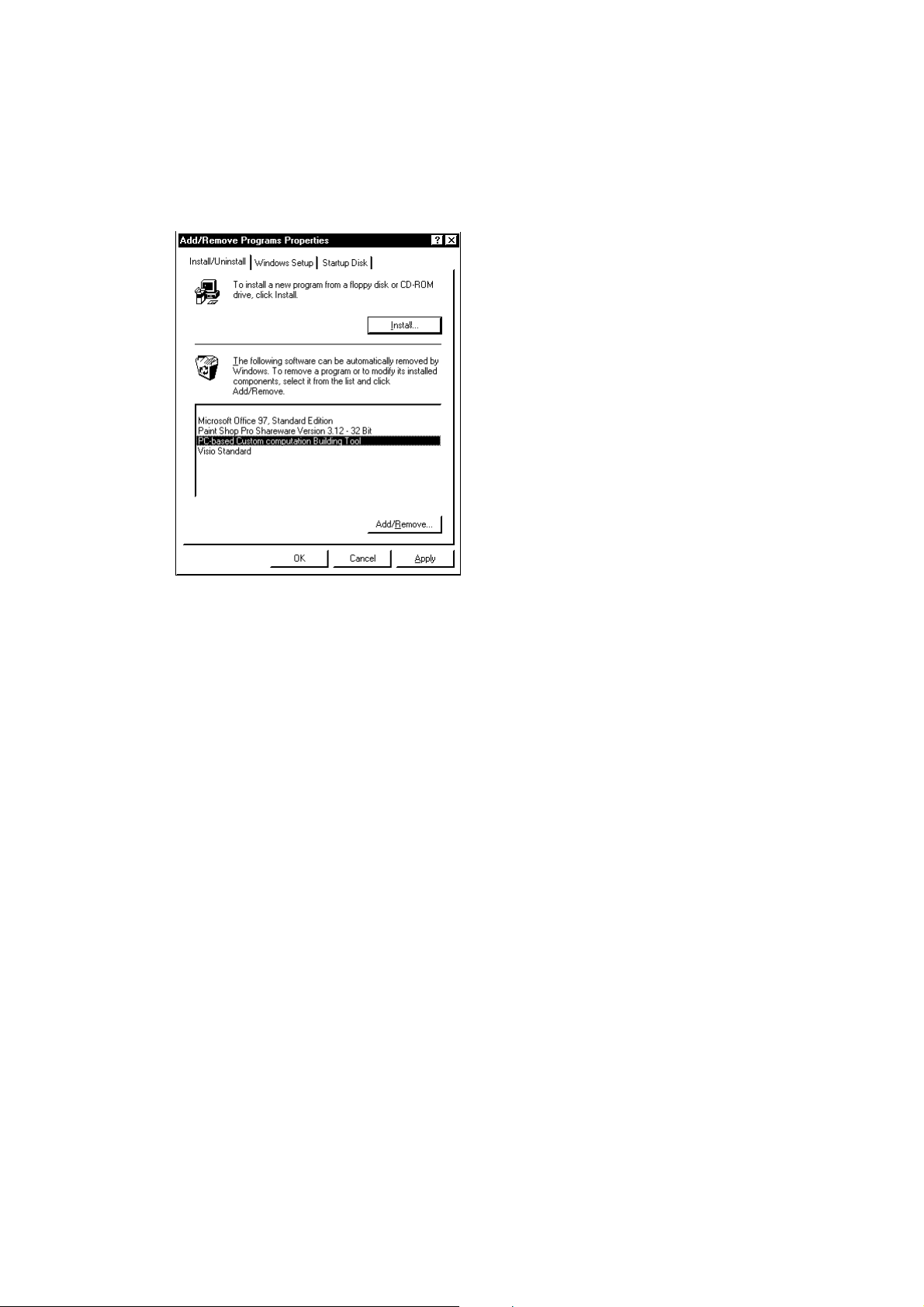
2.2 Uninstalling the LL1200 Tool

(1) Double-click the <Add/Remove Programs> icon in the Control Panel menu of Windows. (2) Choose <LL1200>, and then click the <Add/Remove . . .> button. (3) To continue, follow the instructions given in each dialog box.

Figure 2.2.1 Dialog Box for Uninstallation Operations

2-4

IM 5G1A11-01E

Chapter 2 Setup

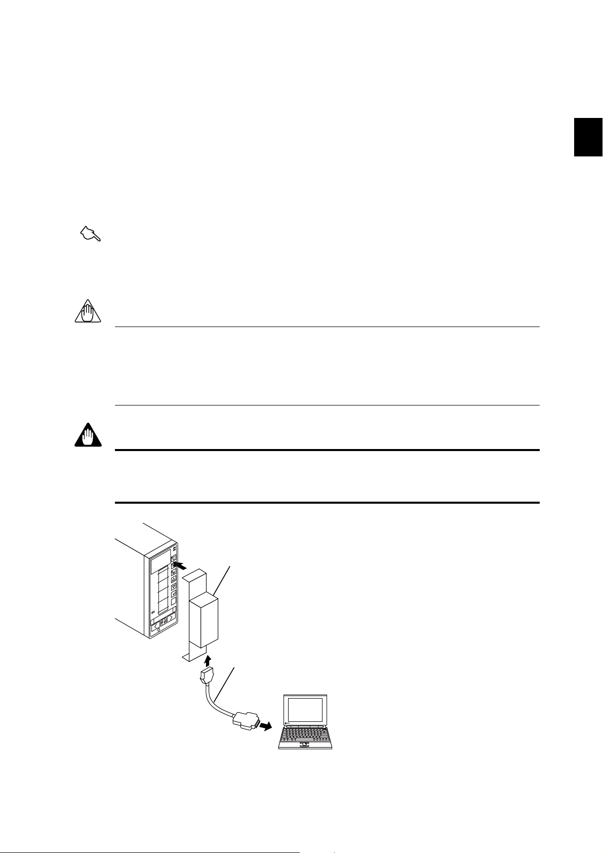
2.3 Connecting the US1000 Controller to the Personal Computer

The US1000 controller can be connected to a personal computer in two ways; using either the optical communication interface on the controller’s front panel or the RS-485 communication terminal on the rear panel (if the US1000 controller has the “/A10” option). This section discusses the way the US1000 controller is connected to the personal computer using the optical communication interface. Connect the controller to the computer either before or after you configure the custom computations. See Section 3.2, “Flow of Working with the LL1200 Tool,” for more information.

See Also

Chapter 1, “Setup,” in the US1000 Digital Indicating Controller-Communication Functions instruction manual (IM 5D1A01-10E), for details on how to wire the US1000 controller using the RS-485 communication terminal.

NOTE

The dedicated adapter has an internal switch (located where the adapter comes into contact with the US1000 controller). Exercise care to avoid breaking the switch when attaching the adapter onto the US1000 controller. Installing the adapter in place automatically turns on the switch, causing the batteries to discharge even if no communication is done. If you have no immediate plan to communicate, keep the adapter removed from the US1000 controller.

WARNING

When using an external power source, take care to ensure that the polarities of the AC adapter are correct. Do not apply power from the AC adapter in excess of the power ratings of the dedicated adapter. Either of these cases may result in damage to the controller.

ALM LP2

SV MV

100

Controller

DISP

YOKOGAWAÅŸ

Dedicated Adapter (Optical/electrical signal converter)

Dedicated cable

Personal computer

To RS-232C terminals

Figure 2.3.1 Connection of the US1000 Controller to the Personal Computer using the

Optical Communication Interface

IM 5G1A11-01E 2-5

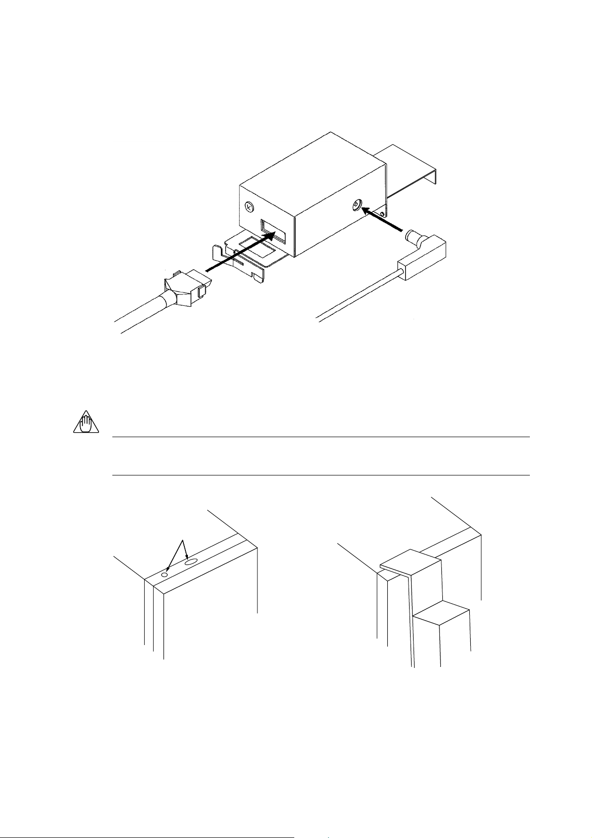
Follow the steps below to connect the dedicated adapter to the US1000 controller. (1) Wire the dedicated adapter to the RS-232C communication port on the personal computer using the

dedicated cable.

Dedicated Cable

Power supply plug

Figure 2.3.2 Connection of the Dedicated Cable to the Dedicated Adapter

(2) Hang the dedicated adapter on the top notches of the US1000 controller, as shown in Figure 2.3.3. (3) Push the adapter on to the controller’s front panel so it is securely fixed.

NOTE

Communication is not possible if the dedicated adapter on the US1000 controller is not horizontally aligned in the correct position. Install the adapter in an upright position on the US1000 controller.

Notch

2-6

Figure 2.3.3 Installation of the Dedicated Adapter

IM 5G1A11-01E

3. Using the LL1200 Tool

This chapter explains how to use the LL1200 tool. Be sure to read this chapter before you proceed any further.

Chapter 3 Using the LL1200 Tool

3.1 Starting and Exiting the Tool

3.1.1 Starting the Tool

(1) From the Start menu of Windows, choose <Programs>, then <LL1200>. (2) The LL1200 tool starts up and the following dialog box appears.

Figure 3.1.1 Dialog Box that Appears When the LL1200 Tool Starts Up

IM 5G1A11-01E 3-1

3.1.2 Exiting the Tool

(1) From the LL1200 tool menus, choose <File>, then <Exit>. (2) The following message box appears.

To save the data of your current work, click the <Yes> button and save the file. If the data need not be saved, click the <No> button.

Figure 3.1.2 [Exit LL1200 Tool] Message Box

3-2

IM 5G1A11-01E

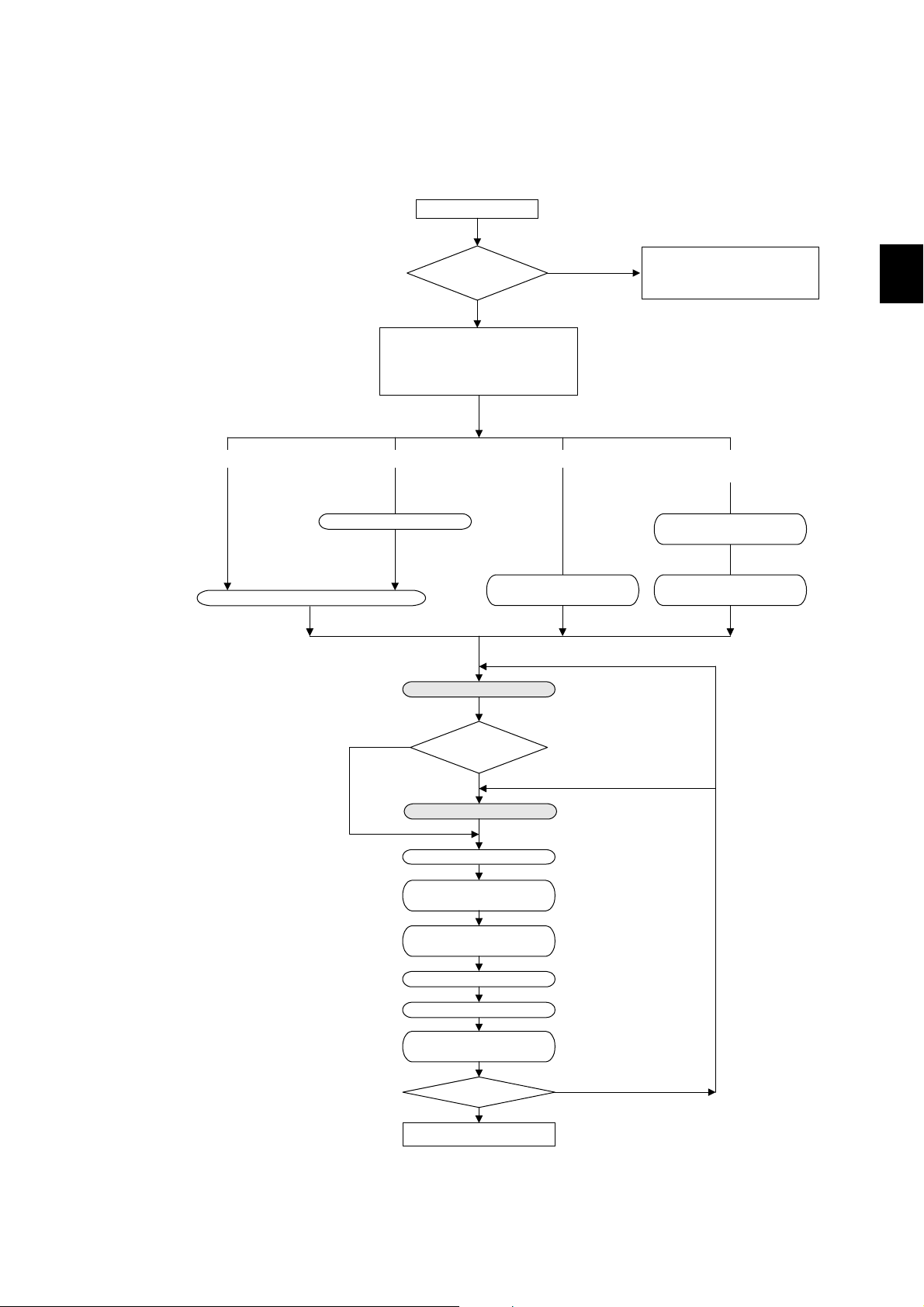
3.2 Flow of Working with the LL1200 Tool

Figure 3.2.1 shows the flow of work for configuring custom computations and displays.

Startup of LL1200 tool

Custom computation or

parameter setting?

Configuration of custom computations

Uploading data from US1000 controller?

Opening user file?

Opening sample file?

Creating new file?

Parameter setting

(Section 4.1)

Chapter 3 Using the LL1200 Tool

See the

Model LL1100 PC-based

Parameters

Setting Tool instruction

manual (IM 5G1A01-01E)

(Creating new file) (Opening sample file) (Opening user file) (Uploading data from

US1000 controller)

(Subsection 7.3.1)

Open a sample file

Connect the US1000 controller

(Section 2.3)

to a personal computer

(Section 8.1)(Subsection 7.3.1)

(Section 4.1)

Specify the suffix code and controller type

Configure the custom computations

Configure the custom displays

Save data in the user file

Connect the US1000 controller

to the personal computer

Open a user file of

custom computations

Configuring custom

displays?

Yes

(Modifying custom computations)

(Chapter 4)

(Modifying custom displays)

(Chapter 5)

(Subsection 7.3.2)

(Section 2.3)

Upload custom-computation data

from the US1000 controller

Download data to the

US1000 controller

Set parameters.

Print (if necessary)

Check the custom computation

monitor/custom displays

Modify

End of work

(Section 8.2)

(Chapter 10)

(Chapter 9)

(Chapter 11)

(Modify)

Figure 3.2.1 Flow of Work for Configuring US1000 Functions Using the LL1200 Tool

IM 5G1A11-01E 3-3

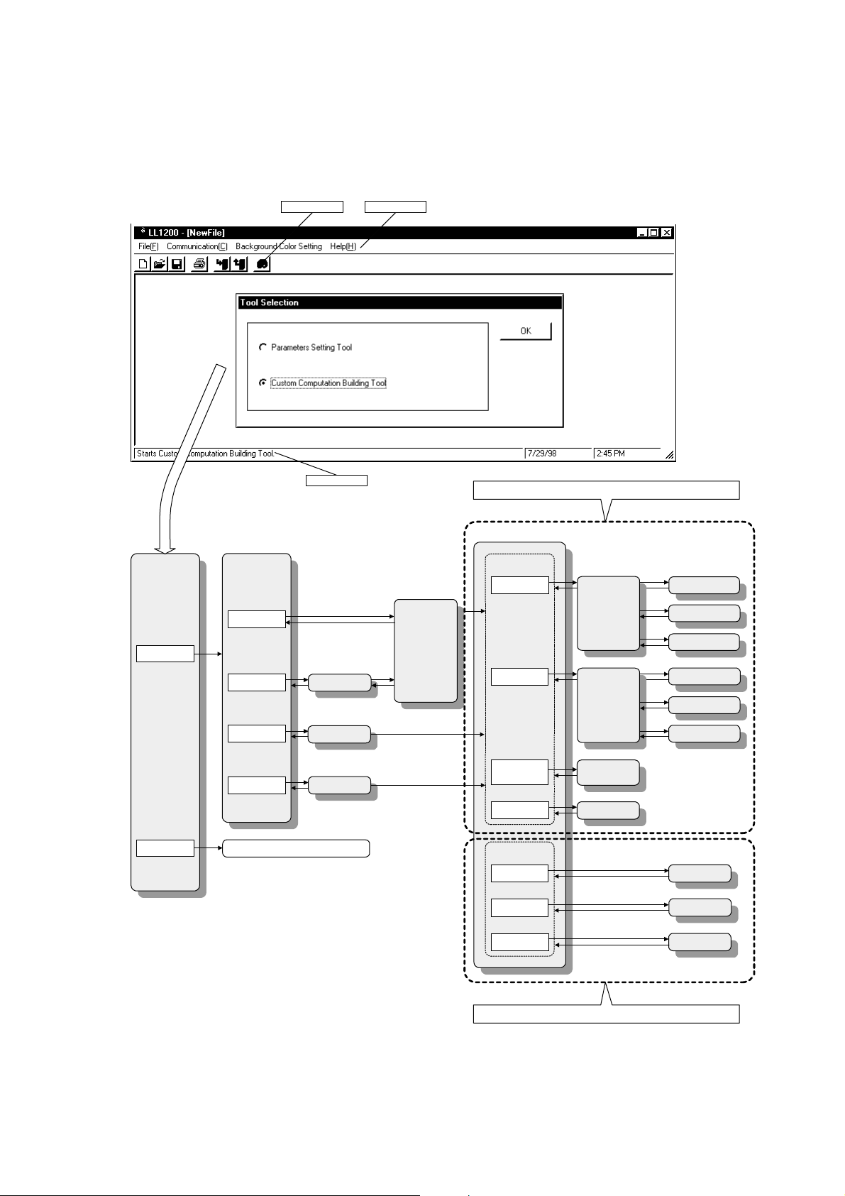
3.3 Dialog Boxes and Tool Menus

Figures 3.3.1 and 3.3.2 show how the dialog boxes and tool menus are organized within the LL1200 tool.

Tool Selection

Custom computation

building tool

New/Modification

New File

Open Sample File

Open User File

Upload from

US1000 Controller

Toolbar

Status bar

(Subsection 7.3.1)

Open

(Sample file)

(Subsection 7.3.1)

Open

(User file)

(Section 8.1) Upload from

US1000 Controller

Tool menus

Specify Suffix Code and Controller Type

Dialog boxes that appear when custom computations are configured

➀

Custom Computation

Configuration Menu

Input Block

Output Block

Ten-segment

Linearizer 3 and 4

Parameters

USER

Parameters

(Section 4.2)

Input Block

(Section 4.3)

Output Block

(Section 4.4)

Parameter Setting for

Ten-segment

Linearizers 3 and 4

(Section 4.5)

USER Parameters

Definition

(Subsection 4.2.1)

Module Configuration

(Subsection 4.2.2)

Module Setting

(Subsection 4.2.3)

Setting of Input Block

Connection Assignment

(Subsection 4.3.1)

Module Configuration

(Subsection 4.3.2)

Module Setting

(Subsection 4.3.3)

Setting of Output Block

Connection Assignment

3-4

Parameters

setting tool

Model LL1100 PC-based Parameters Setting

instruction manual (IM 5G1A01-01E)

Tool

Figure 3.3.1 Paths for Moving among Dialog Boxes

Custom Display

Configuration Menu

Custom Display

Selection

Custom Display

Switching Condition

Security Definitions

(Subsection 5.2.1)

Custom Display

Selection

(Subsection 5.2.2) Custom Display

Switching Conditions

(Section 5.3)

Security Definition

Dialog boxes that appear when custom displays are configured

IM 5G1A11-01E

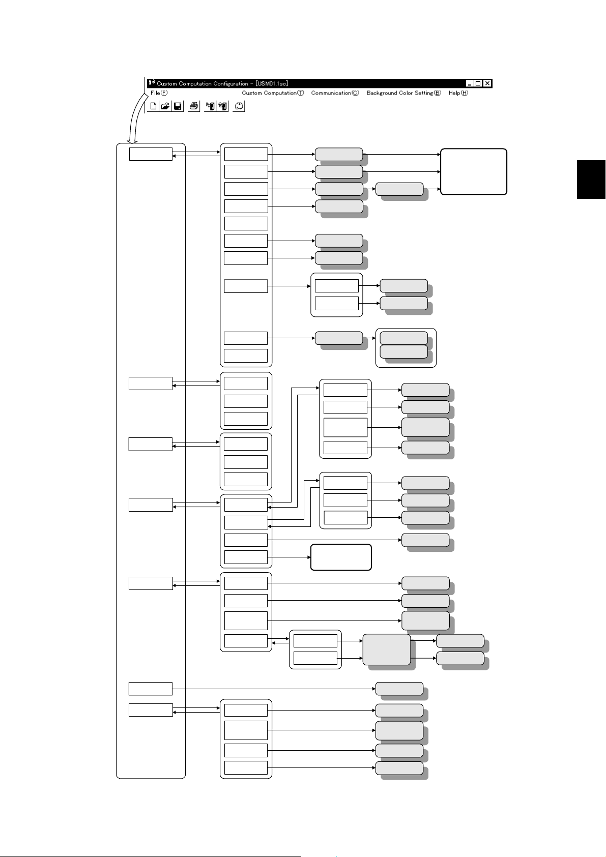
Tool menus

File

New

Open

Open Sample File

Save

Save As

Compare

Specify Suffix Code and Controller Type

Open

(User file)

Open

(Sample file)

Main Window

Save As

Compare

Specify Suffix Code and Controller Type

Chapter 3 Using the LL1200 Tool

Choosing any of these options switches to the window marked ➀ in Figure 3.3.1. For information on the subsequent windows, see the paragraphs describing the way the windows are organized.

Editing

Modify Configuration

Display Vertical Division

Horizontal Division

Custom Computation

Communication

Background

Color Setting

Help

Custom Computation

Custom Display

Configuration

Controller Type

Start Parameters

US1000 Controller

Custom Computation

Description of

Module Information

Version Information

Information

Exit

Connection

Delete

Cancel

Configuration

Changing of

Setting Tool

Download to

Upload from

Compare

Monitor

Building Tool

D-registers

and I-relays

File Information

I/O Signal Information

(Chapter 9)

Setting of Print Range

Input Block

Output Block

Ten-segment

Linearizers 3 and 4

Parameters

USER Parameters

Display Selection

Display Switching

Condition

Security Definition

Exit the custom computation building tool and start the parameters setting tool.

Input Block

Output Block

File Information

I/O Signal Information

Setting

Printer Setting

Print Preview

(Chapter 10)

Communication

Condition Setting

Background Color

Setting

Custom Computation

Building Tool

Description of

D-registers

and I-relays

Description of

Module Information

Version Information

Input Block

Output Block

Parameter Setting for

Ten-segment

Linearizer 3 and 4

USER Parameters

Custom Display

Selection

Custom Display

Switching Conditions

Security Definition

Specify Suffix Code and Controller Type

Download to

US1000 Controller Upload from US1000

Controller

Compare with

US1000 Controller's

Custom Data

Input Block Monitor

Output Block Monitor

(Chapter 8)

(Chapter 11)

Figure 3.3.2 Paths for Moving among the Options in the Tool Menus

IM 5G1A11-01E 3-5

Chapter 4

Basic Operations for Configuring Custom Computations and Relevant Explanations

This chapter explains the procedure for configuring custom computations. For details on the preparatory work for using the LL1200 tool, see Chapter 2, "Setup." Likewise, for

an overview of the procedure for configuring custom computations and displays, see Chapter 3, "Using the LL1200 Tool."

Also refer to Chapter 4, "List of Computation Modules and Their Functions," in the Model LL1200 PC-based Custom Computation Building Tool-User's Reference instruction manual (IM 5G1A11-02E), for detailed specifications of the computation modules.

In order to configure custom computations, you must follow the steps shown below.

●Step 1: Choosing the Way Computations Are Configured --------------------------- (Section 4.1)

●Step 2: Configuring Custom Computations in an Input Block ----------------------- (Section 4.2)

●Step 3: Configuring Custom Computations in an Output Block --------------------- (Section 4.3)

●Step 4: Setting Ten-segment Linearizers 3 and 4 Parameters (as necessary)- (Section 4.4)

●Step 5: Setting USER Parameters (as necessary) ------------------------------------- (Section 4.5)

When you are finished with these steps, download the configured custom computations to the US1000 controller (see Section 8.2). Then, verify their performance by means of custom computation monitoring (see Chapter 11).

IM 5G1A11-01E 4-1

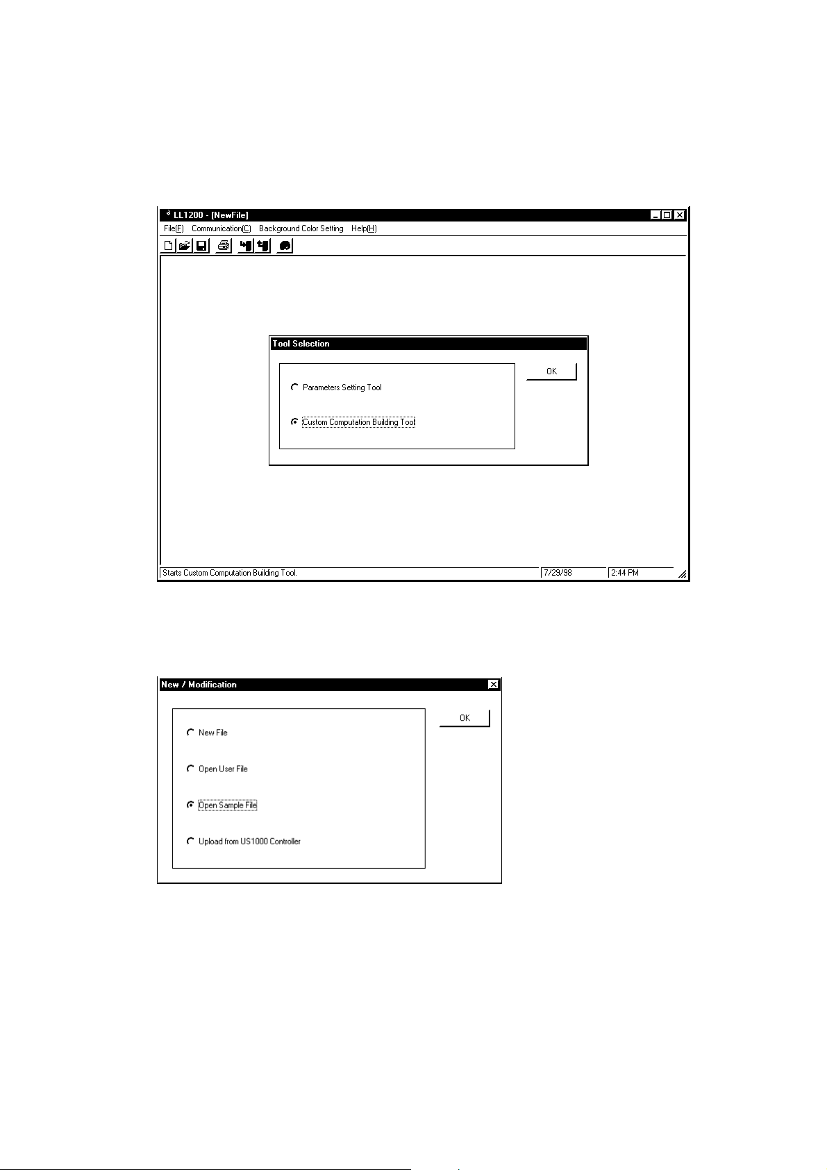
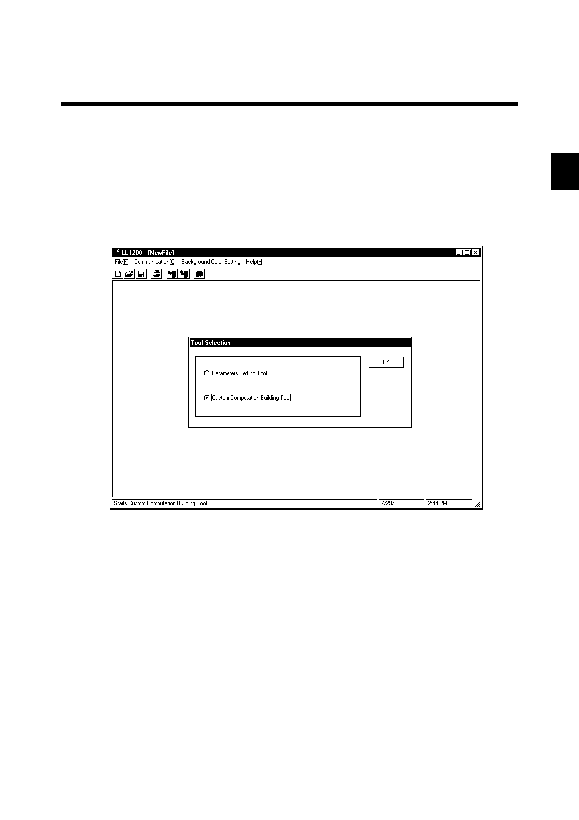
4.1 Step 1: Choosing the Way Computations Are Configured

When you start the LL1200 tool, a dialog box appears as shown in Figure 4.1.1.

Figure 4.1.1 [Tool Selection] Dialog Box

Click the <Custom Computation Building Tool> option button, and then the <OK> button. The [New/ Modification] dialog box (Figure 4.1.2) appears.

Figure 4.1.2 [New/Modification] Dialog Box

4-2

IM 5G1A11-01E

Chapter 4

There are four ways of configuring custom computations, as described below. Choose one of these four ways.

TIP

If you are configuring custom computations for the first time, it is advisable that you use a sample file. For your information, Section 4.2, “Step 2: Configuring Custom Computations in an Input Block,”

uses the sample file (USM01.1SC) for single-loop control to explain all the operating procedures that follow that particular section.

Basic Operations for Configuring Custom Computations and Relevant Explanations

① If you are configuring a custom computation from scratch, choose <New File>.

Click the <New File> option button, then the <OK> button. The [Specify Suffix Code and Controller Type] dialog box (Figure 4.1.3) appears.

② If you are configuring a custom computation using a user file, choose <Open User File>.

Click the <Open User File> option button, and then the <OK> button. The [Open User File] dialog box (Figure 4.1.4) appears.

③ If you are configuring a custom computation using a sample file, choose <Open Sample File>.

Click the <Open Sample File> option button, and then the <OK> button. The [Open Sample File] dialog box (Figure 4.1.5) appears.

④ If you are configuring a custom computation by uploading data from the US1000 controller,

choose <Upload from US1000 Controller>. Click the <Upload from US1000 Controller> option button, and then the <OK> button. The [Upload from US1000 Controller] dialog box (Figure 4.1.6) appears.

NOTE

When uploading custom computation information from US1000 controller, set the controller mode (US mode) to “21.”

IM 5G1A11-01E 4-3

■ [Specify Suffix Code and Controller Type] Dialog Box

If you choose <New File> in the [New/Modification] dialog box (Figure 4.1.2), the [Specify Suffix Code and Controller Type] dialog box (Figure 4.1.3) appears. This dialog box also appears if you choose <Open Sample File>. In the [Specify Suffix Code and Controller Type] dialog box, click the <OK> button. The [Custom Computation Configuration Menu] dialog box (Figure 4.1.7) appears.

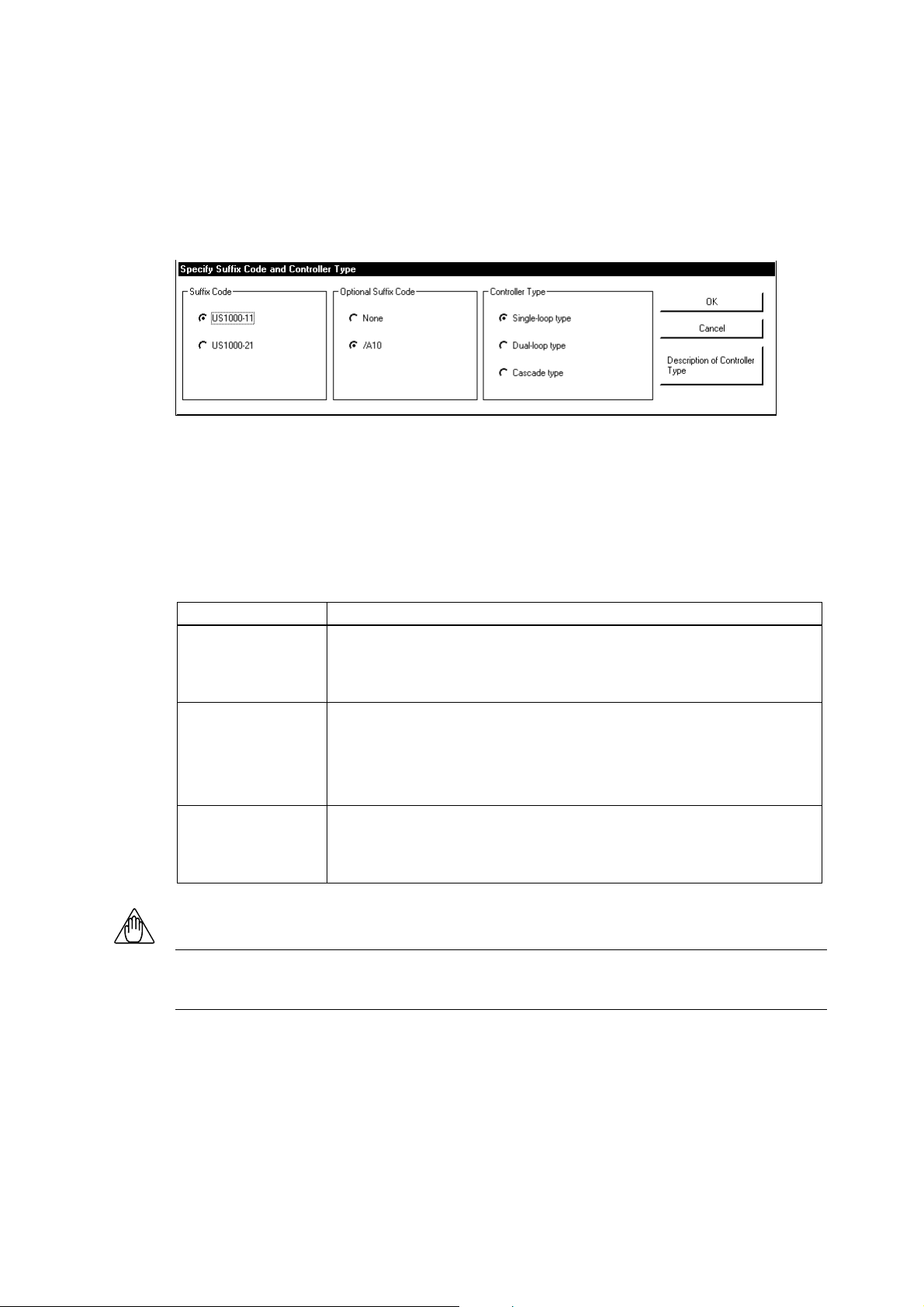
Figure 4.1.3 [Specify Suffix Code and Controller Type] Dialog Box

● Explanation of the [Specify Suffix Code and Controller Type] Option

The suffix code must be specified because the code needs to be verified when you download information on the custom computations you configured using the LL1200 tool, to the US1000 controller. Likewise, the controller type must be specified because you must decide upon the desired operating conditions for the US1000 controller.

Criteria for ChoiceController Type

Single-loop type

Dual-loop type

Cascade type

The following are used:

• One PID computation

• Switching among loop-1 CAS, AUTO and MAN modes

• Switching between RUN/STOP modes

• Switching between the loop-1 Open/Close modes The following are used:

• Two PID computations

• Switching among loop-1 CAS, AUTO and MAN modes

• Switching among loop-2 CAS, AUTO and MAN modes

• Switching between RUN/STOP modes

• Switching between the loop-1 Open/Close modes

• Switching between the loop-2 Open/Close modes The following are used:

• Two PID computations

• Switching between RUN/STOP modes

• Switching among the loop-1 CAS, AUTO and MAN modes

• Switching between the loop-2 Open/Close modes

NOTE

Data cannot be downloaded to US1000 controllers whose suffix codes do not match the one specified. Check the suffix and optional suffix codes of the US1000 controller to which you download data.

4-4

IM 5G1A11-01E

■ Open User File

In the [Open User File] dialog box, choose the file you wish to use and click the <Open> button. The [Custom Computation Configuration Menu] dialog box (Figure 4.1.7) appears.

Figure 4.1.4 [Open User File] Dialog Box

■ Open Sample File

In the [Open Sample File] dialog box, choose the file you wish to use and click the <Open> button. The [Specify Suffix Code and Controller Type] dialog box (Figure 4.1.3) appears. In the dialog box, click the <OK> button. The [Custom Computation Configuration Menu] dialog box (Figure 4.1.7) appears.

Chapter 4

Basic Operations for Configuring Custom Computations and Relevant Explanations

Figure 4.1.5 [Open Sample File] Dialog Box

IM 5G1A11-01E 4-5

■ Upload from US1000 Controller

If you choose <Upload from the US1000 Controller> in the [New/Modification] dialog box, the [Upload from US1000 Controller] dialog box (Figure 4.1.6) appears.

Option button

Drop-down list box

Figure 4.1.6 [Upload from US1000 Controller] Dialog Box

You can communicate with the US1000 controller in either of the following two ways.

●Communication Using the Front-panel Optical Interface ① In the [Upload from US1000 Controller] dialog box, click the <Front Terminal> option button. ② From the <Serial Port> drop-down list box, choose either COM1, COM2, COM3 or COM4. ③ Click the <Execute> button. Data are uploaded from the US1000 controller. ④ When uploading is complete, the [Custom Computation Configuration Menu] dialog box (Figure

4.1.7) appears.

⑤ For the subsequent operations, see Section 4.2 and the sections/subsections that follow.

●Communication Using the RS-485 Interface ① In the [Upload from US1000 Controller] dialog box, click the <Rear Terminal> option button. ② From the <Serial Port> drop-down list box, choose either COM1, COM2, COM3 or COM4. Then,

from the <Baud Rate>, <Parity> and <Address> drop-down list boxes, choose the options of the three communication conditions, the baud rate, parity and address. Also choose the options of the two communication conditions, the stop bit and data length, by clicking the appropriate option buttons in the <Stop Bit> and <Data Length> sections. Match the communication conditions of the US1000 controller with those of the personal computer.

③ Click the <Execute> button. The LL1200 tool begins uploading data from the US1000 controller. ④ When uploading is complete, the [Custom Computation Configuration Menu] dialog box (Figure

4.1.7) appears.

⑤ For the subsequent operations, see Section 4.2 and the sections/subsections that follow.

4-6

NOTE

If you have chosen RS-485 communication, set the communication protocol of the US1000 controller to [PC-link Communication]. Communication is not possible if you set the protocol to [PC-link Communication with Sum Check], [Modbus (RTU)] or [Modbus (ASCII)].

IM 5G1A11-01E

Chapter 4

■ Custom Computation Configuration Menu

The dialog box shown below is the first to appear when you configure custom computations. For further operations after this Custom Computation Configuration Menu dialog box, see Section 4.2 and the sections/subsections that follow.

Basic Operations for Configuring Custom Computations and Relevant Explanations

Options in Custom Computation Configuration Menu

Figure 4.1.7 [Custom Computation Configuration Menu] Dialog Box

IM 5G1A11-01E 4-7

4.2 Step 2: Configuring Custom Computations in an Input Block

The flow of work in step 2 is as follows.

This section explains the work flow using the single-loop control sample file (USM01.1SC). Read the sample file onto your personal computer before you start this step.

Start of custom computation

configuration

Configure the inputs and parameters

of computation modules

Connect the input block to the control

and computing section

Set the analog-input burnout prevention

function (as necessary)

End of custom computation

configuration

(Subsection 4.2.1)

(Subsection 4.2.2)

(Subsection 4.2.3)

(Subsection 4.2.4)

Figure 4.2.1 Flow of Work for Configuring Custom Computations in an Input Block

Figure 4.2.2 shows the [Custom Computation Configuration Menu] dialog box used to configure custom computations.

Option chosen to configure custom computations in an input block

4-8

Figure 4.2.2 [Custom Computation Configuration Menu] Dialog Box

IM 5G1A11-01E

Chapter 4

Basic Operations for Configuring Custom Computations and Relevant Explanations

4.2.1 Step 2-1: Registering Computation Modules

- Explanation

This step involves registering the computation modules you want to perform operations in an input block, in the order they are executed. You can register a maximum of 30 computation modules.

Figure 4.2.3 shows an input block for single-loop control where a module for a logical “NOT” operation is added. The following paragraphs explain how to add a NOT module to the diagram of an input block for single-loop control.

Computation module

ranked first in the

order of execution

(i.e., first-run module)

Computation module

ranked

second

third

in the

order of execution

(i.e., second-run module)

Computation module

ranked

order of execution

(i.e., third-run module)

PV input

IN1

P1=0 (AIN1)

41:EUCONV

33:PLINE1

PVIN. 1 R/S

P2=0 (PV1)

1401

IN1

1403

41:EUCONV

feedforward input

IN1

1405

CSVIN. 1

Cascade or

AIN3AIN1

13031301

P1=2 (AIN3) P2=0 (PV1)

Control and computing section

Output block

SV number selection

AUT1 MAN1

R/S

DI1. st

DI2. st DI3. st DI4. st DI5. st DI6. st DI7. st

5161

5162 5163 5164 5165 5166 5167

NOT module registered as one

IN1

17:NOT

1407

AUT. 1

ranked fourth in the order of execution (i.e., fourth-run module)

MAN. 1

SV. B0 SV. B1

SV. B2

SV. B3

Input block

Figure 4.2.3

Addition of a NOT Module to the Diagram of an Input Block for Single-loop Control

IM 5G1A11-01E 4-9

- Operation: Registering the Modules

TIP

Computation modules can be positioned anywhere within the input block. You should however locate them as close as possible to the input signals (AIN1 to AIN3 and DI1.st to DI7.st) for the input block connected to the modules. This strategy makes wiring between module I/Os visible and simple.

① In the [Custom Computation Configuration Menu] dialog box (Figure 4.2.2), click the <Input

Block> button. The [Input Block] dialog box appears. Figure 4.2.4 illustrates the [Input Block] dialog box for single-loop control.

4-10

Figure 4.2.4 [Input Block] Dialog Box for Single-loop Control

② In the [Input Block] dialog box, double-click a blank box. The [Module Configuration] dialog box

(Figure 4.2.5) appears. For ease of selection, modules are classified into four types; arithmetic operation, logical operation, special operation and special function.

IM 5G1A11-01E

Chapter 4

Basic Operations for Configuring Custom Computations and Relevant Explanations

Indexes

Figure 4.2.5 [Module Configuration] Dialog Box

③ Click the index that contains the computation module you register. ④ Double-clicking the module registers it.

Figure 4.2.6 shows an example where the <17: NOT> option in the <Logical Operation> index is registered.

Indicates the registered NOT module

Figure 4.2.6 Example where a NOT Module Is Registered as the Fourth-Run Module

IM 5G1A11-01E 4-11

TIP

To view an explanation on the selected module, click the right mouse button in the [Module Configuration] dialog box. And then click the [Module Description]. The [Custom Computation Module Help for US1000] view appears. Figure 4.2.7 shows an explanation on a NOT module.

Figure 4.2.7 [Custom Computation Module Help for US1000] View

Repeat steps ② to ④ to register other necessary computation modules also.

When you have finished registering modules, proceed to subsection 4.2.2, “Step 2-2: Configuring the Inputs and Parameters of Computation Modules.”

4-12

IM 5G1A11-01E

Chapter 4

Basic Operations for Configuring Custom Computations and Relevant Explanations

4.2.2 Step 2-2: Configuring the Inputs and Parameters of Computation Modules

- Explanation

Each computation module has inputs (8 maximum), parameters (4 maximum) and an output. This step involves configuring inputs and parameters only. The results of computation provided by the output are automatically stored, according to the module’s order of execution, in the data storage area of the US1000 controller.

Inputs (8 maximum)

• • •

IN1 IN2

OUT

Output (one)

Module

No. xx

IN8

• • •

Parameters

(4 maximum)

Figure 4.2.8 Conceptual View of Module Configuration

IM 5G1A11-01E 4-13

As was the case in the previous subsection, Figure 4.2.9 shows an input block for single-loop control where a logical NOT operation module is added. In this block diagram, analog input 1 (AIN1) is connected to the input of an EUCONV module ranked first in the order of execution. Since the EUCONV module requires parameters, a constant data value of 0 is set for both parameters P1 and P2. For more information on the handling of P1 and P2 parameters, see Chapter 4, “List of Computation Modules and Their Functions,” in the Model LL1200 PC-based Custom Computation Building Tool- User’s Reference instruction manual (IM 5G1A11-02E). The output of the EUCONV module, which is ranked first in the order of execution, is connected to the input of the PLINE1 module which is ranked second in the order of execution. The PLINE1 module has no parameters. Analog input AIN3 is connected to the input of the EUCONV module ranked third in the order of execution. The constant data values of 2 and 0 are set in parameters P1 and P2 of the EUCONV module. In addition, contact input 1 is connected to the input of the NOT module which was registered in the previous subsection and is ranked fourth in the order of execution.

Input of PLINE1 module

Input and parameters of EUCONV module

PV input

IN1

P1=0 (AIN1)

41:EUCONV

33:PLINE1

PVIN. 1 R/S

P2=0 (PV1)

1401

IN1

1403

feedforward input

IN1

41:EUCONV

1405

CSVIN. 1

Cascade or

AIN3AIN1

13031301

P1=2 (AIN3) P2=0 (PV1)

Control and computing section

Contact input 1 (DI1) is connected to the input of the NOT module

AUT1 MAN1

R/S

DI1. st

DI2. st DI3. st DI4. st DI5. st DI6. st DI7. st

5161

5162 5163 5164 5165 5166 5167

IN1

17:NOT

1407

Input and parameters of EUCONV module

MAN. 1 SV. B0 SV. B1

AUT. 1

SV number

selection

SV. B2

SV. B3

Input block

4-14

Output block

Figure 4.2.9 Contact Input 1 Connected to the Input of the NOT Module

IM 5G1A11-01E

Chapter 4

Basic Operations for Configuring Custom Computations and Relevant Explanations

- Operation: Configuring the Modules

This operation involves configuring the inputs and parameters of the computation modules. ① In the [Input Block] dialog box, click the module whose inputs and parameters you want to

configure. In the example shown in Figure 4.2.6, click the NOT module.

② From the tool menus, choose <Editing>, then <Connection>.

The [Module Setting] dialog box (Figure 4.2.10) appears.

Indexes

Figure 4.2.10 [Module Setting] Dialog Box

③ Click the input from among <IN1> to <IN8> or the parameter from among <P1> to <P4>, that

need to be configured.

④ Click the appropriate index.

Indexes are classified into <AINn>,<DIn.st>, <Module Output>, <D-register>, <I-relay> and <Constant Value>.

IM 5G1A11-01E 4-15

●Description of Indexes

Index Remarks

AINn

DIn.st

Module Output

D-Register

I-Relay

Constant Value

AIN1: Analog Input 1 AIN2: Analog Input 2 AIN3: Analog Input 3

DI1.st: Contact Input 1 DI2.st: Contact Input 2 DI3.st: Contact Input 3 DI4.st: Contact Input 4 DI5.st: Contact Input 5 DI6.st: Contact Input 6 DI7.st: Contact Input 7

IMO1L to IMO30L (outputs of input-block computation modules) OMO1L to OMO30L (outputs of output-block computation modules)

Process data, mode data, operation parameters, setup parameters

ON/OFF status, ON status, OFF status, SVNO, PIDNO, timer flags, power-on flags, alarm flags, etc.

Configurable range: -19999 to 30000

Description

Analog input data fed to input block

Contact input data fed to input block

See Appendix 4, “Areas for Storing Data Output from Computation Modules.”

See Sections 5.3 to 5.9 in the Model

LL1200 PC-based Custom Computation Building Tool—User’s Reference

instruction manual (IM 5G1A11-02E). See Sections 5.10 to 5.13 in the Model

LL1200 PC-based Custom Computation Building Tool—User’s Reference

instruction manual (IM 5G1A11-02E).

⑤ Double-clicking the appropriate input source configures the selected index.

To configure the <Constant Value> index, type a value in the text box, and then press the <Enter> key. The figure below shows an example of how to configure contact input 1 <DI1.st>.

➀ Click <IN1>

➁ Click the <DIn.st> index

➂ Click <DI1.st>.

Figure 4.2.11 Configuring Contact Input 1 <DI1.st>

⑥ Repeat steps ③ to ⑤ to configure the other necessary inputs among <IN1> to <IN8> or parameters

among <P1> to <P4>.

⑦ Clicking the <OK> button closes the [Module Setting] dialog box. When the dialog box closes,

the computation modules are automatically wired according to the inputs and parameters you configured.

⑧ Repeat steps ① to ⑦ to configure other computation modules also.

4-16

IM 5G1A11-01E

Chapter 4

Basic Operations for Configuring Custom Computations and Relevant Explanations

When you have finished configuring the inputs and parameters of computation modules, proceed to subsection 4.2.3, “Step 2-3: Connecting Computation Modules to the Control and Computing Section.”

4.2.3 Step 2-3: Connecting Computation Modules to the Control and Computing Section

- Explanation

This step involves making the settings needed to pass the results of computation to the control and computing section after completing the module configuration and settings discussed so far.

As was the case in the previous subsection, Figure 4.2.12 shows an input block for single-loop control where a logical NOT operation module is added.

In this block diagram, the output of the ten-segment linearizer 1 (PLINE1) module ranked second in the order of execution is connected to the loop-1 PV input (PVIN.1). The output of the EU range conversion (EUCONV) module ranked third in the order of execution is connected to the loop-1 cascade input (CSVIN.1). AIN3 is connected to the feedforward input (FF). In addition, the output of the NOT module ranked fourth in the order of execution is connected to the RUN/STOP mode (R/S) output signal.

PV input

IN1

41:EUCONV

1401

IN1

33:PLINE1

1403

P1=0 (AIN1) P2=0 (PV1)

feedforward input

IN1

41:EUCONV

1405

Cascade or

AIN3AIN1

13031301

P1=2 (AIN3) P2=0 (PV1)

AUT1 MAN1

R/S

DI1. st

DI2. st DI3. st DI4. st DI5. st DI6. st DI7. st

5161

5162 5163 5164 5165 5166 5167

The AIN3 input signal is passed to the FF output signal

IN1

17:NOT

1407

The output from the NOT module is passed

to the R/S output signal

SV number selection

Input block

SV. B3

SV. B2

The output from the PLINE1 module is passed to the PVIN.1 output signal

PVIN. 1 R/S

The output from the EUCONV module is passed to the CSVIN.1 output signal

CSVIN. 1

Control and computing section

Output block

AUT. 1

MAN. 1

SV. B0 SV. B1

Figure 4.2.12 Connection of the NOT Module’s Output to the Control and Computing

Section

IM 5G1A11-01E 4-17

- Operation: Connecting to the Control and Computing Section

This operation involves making the settings needed to pass the results of computation in the input block to the control and computing section.

① In the [Input Block] dialog box (Figure 4.2.13), click the appropriate output signal. Click <R/S> in

the example shown in Figure 4.2.13.

Output signals fed by the input block

Figure 4.2.13 Output Signals Fed by the Input Block

4-18

IM 5G1A11-01E

Chapter 4

Basic Operations for Configuring Custom Computations and Relevant Explanations

●Description of Output Signals Fed by the Input Block

Output Signal Fed by Input Block Description

PVIN.1 PVIN.2 CSVIN.1 CSVIN.2 GAIN.1 GAIN.2

TRK.1 TRK.2 FF CAS.1 AUT.1 MAN.1 CAS.2 AUT.2 MAN.2 O/C R/S TRF.1 TRF.2

Loop-1 PV input Loop-2 PV input Loop-1 cascade input Loop-2 cascade input Loop-1 gain setting value Loop-2 gain setting value

Loop-1 tracking input Loop-2 tracking input Feedforward input Loop-1 CAS mode Loop-1 AUTO mode Loop-1 MAN mode Loop-2 CAS mode Loop-2 AUTO mode Loop-2 MAN mode OPEN/CLOSE mode RUN/STOP mode Loop-1 tracking flag Loop-2 tracking flag

② From the tool menus, choose <Editing>, then <Connection>.

The [Setting of Input Block Connection Assignment] dialog box (Figure 4.2.14) appears.

Indexes

Figure 4.2.14 [Setting of Input Block Connection Assignment] Dialog Box

③ Click the appropriate index.

Indexes are classified into <AINn>,<DIn.st>, <Module Output>, <D-register>, <I-relay> and <Constant Value>.

IM 5G1A11-01E 4-19

●Description of Indexes

Index Remarks

AINn

DIn.st

Module Output

D-Register

I-Relay

Constant Value

AIN1: Analog Input 1 AIN2: Analog Input 2 AIN3: Analog Input 3

DI1.st: Contact Input 1 DI2.st: Contact Input 2 DI3.st: Contact Input 3 DI4.st: Contact Input 4 DI5.st: Contact Input 5 DI6.st: Contact Input 6 DI7.st: Contact Input 7

IMO1L to IMO30L (outputs of input-block computation modules) OMO1L to OMO30L (outputs of output-block computation modules)

Process data, mode data, operation parameters, setup parameters

ON/OFF status, ON status, OFF status, SVNO, PIDNO, timer flags, power-on flags, alarm flags, etc.

Configurable range: -19999 to 30000

Description

Analog input data fed to input block

Contact input data fed to input block

See Appendix 4, “Areas for Storing Data Output from Computation Modules.”

See Sections 5.3 to 5.9 in the Model

LL1200 PC-based Custom Computation Building Tool—User’s Reference

instruction manual (IM 5G1A11-02E). See Sections 5.10 to 5.13 in the Model

LL1200 PC-based Custom Computation Building Tool—User’s Reference

instruction manual (IM 5G1A11-02E).

④ Double-clicking the appropriate input source configures the selected index.

To configure the <Constant Value> index, type a value in the text box, and then press the <Enter> key. The figure below shows an example of how to configure <IMO4L>, the module that is the fourth input-block computation module to be carried out.

Indexes

Figure 4.2.15 Configuring <IMO4L>, the Fourth Input-block Computation Module to Be

Carried Out

⑤ Clicking the <OK> button after the configuration is completed closes the [Setting of Input Block

Connection Assignment] dialog box. When the dialog box closes, the computation modules are automatically wired according to the settings you defined.

⑥ Repeat steps ① to ⑤ to define the connection of other necessary output signals also.

4-20

IM 5G1A11-01E

Chapter 4

Figure 4.2.16 shows the input block with the configuration and setting of computation modules, as well as their connection to the control and computing block, completed.

Basic Operations for Configuring Custom Computations and Relevant Explanations

Figure 4.2.16 Registration of a NOT Module in the Diagram of an Input Block for Single-

loop Control (Finished View)

IM 5G1A11-01E 4-21

4.2.4 Step 2-4: Setting the Analog-input Burnout Function

- Explanation

The US1000 controller has a function designed to switch the output of a loop in use to the preset value in the event of an A/D conversion failure or analog-input burnout. This function is configured in the following step. To use the function, determine which output signal among PV1, PV2, CSV1 and CSV2 should be coupled with signals coming in through the AIN1, AIN2 and AIN3 inputs. In the example shown in the [Connection of Analog Input Burnout Information] dialog box (Figure

4.2.17), AIN1 is coupled with PVIN.1 and AIN3 with CSV.1. This configuration switches the loop-1 MV output value to the preset one if a burnout occurs at either the AIN1 or AIN3 input.

Figure 4.2.17 [Connection of Analog Input Burnout Information] Dialog Box

- Operation

① The [Connection of Analog Input Burnout Information] dialog box appears when you finish

configuring custom computations in the [Input Block] dialog box and click the <OK> button. If you do not need to set any analog-input burnout information, simply click the <OK> button.

② In the [Connection of Analog Input Burnout Information] dialog box, click the appropriate blank

box. A check mark (✔) appears in the box. The setting is complete if the box shows a check mark.

③ When the setting is complete, click the <OK> button. The display returns to the [Custom Compu-

tation Configuration Menu] dialog box (Figure 4.2.2).

If you also want to configure custom computations in the output block after you finish configuring the input-block custom computations, proceed to the next section.

4-22

IM 5G1A11-01E

Chapter 4

Basic Operations for Configuring Custom Computations and Relevant Explanations

4.3 Step 3: Configuring Custom Computations in an Output Block

The flow of work in step 3 is as follows.

Start of custom computation

configuration

Configure the inputs and parameters

of computation modules

Connect the computation modules'

outputs with the output signals

End of custom computation

configuration

(Subsection 4.3.1)

(Subsection 4.3.2)

(Subsection 4.3.3)

Figure 4.3.1 Flow of Work for Configuring Custom Computations in an Output Block

Figure 4.3.2 shows the [Custom Computation Configuration Menu] dialog box used to configure custom computations.

Option chosen to configure custom computations in an output block

Figure 4.3.2 [Custom Computation Configuration Menu] Dialog Box

IM 5G1A11-01E 4-23

4.3.1 Step 3-1: Registering Computation Modules

- Explanation

This step involves registering the computation modules you want to perform operations in an output block, in the order they are executed. You can register a maximum of 30 computation modules.

NOTE

It is recommended that the output blocks included in the US mode of the US1000 be used as they are. The output selection modules listed below can be used to select the output type using the output selection parameter (MVS1 or MVS2). If you make any change to the way an output selection module is connected, the output in question may fail to function correctly. Available output selection modules: OUTSEL1, OUTSEL11, OUTSEL12, OUTSEL13, OUTSEL2 and OUTSEL21

NOTE

When applying time-proportional PID computation, do not allow the computation to be carried out between the output selection module and an output signal (OUT1A, OUT2A, OUT1R or OUT2R).

Figure 4.3.3 shows an output block for single-loop control where a logical OR operation module is added. The following paragraphs explain how to add an OR module to the diagram of an output block for single-loop control.

These signals are automatically connected according to the setting in the MV output selection parameter (MVS1 setup parameter)

Computation module

ranked first in the order of execution (i.e., first-run module)

Computation module

ranked second in the

order of execution

(i.e., second-run module)

Computation module

ranked third in the order of execution

(i.e., third-run module)

Control and computing section

HMV. 1 CMV. 1MV. 1 RET1

1505

1507 1509 1511 1512

ALO13 ALO14

5691 5693

IN1 IN2 IN3 IN4

46:OUTSEL1

47:OUTSEL11348:OUTSEL12449:OUTSEL13

1603 1605

OUT1A

OUT2A OUT2ROUT1R

IN5 IN6 IN7

1601

1607

Computation module

ranked fourth in the

order of execution

(i.e., fourth-run module)

Input block

The OUTSEL1, OUTSEL11, OUTSEL12 and OUTSEL13 modules must always be used together as a set when you use the MV output as a time-proportional output or heating/cooling output

RET2

OR module registered as one ranked sixth in the order of execution (i.e., sixth-run module)

OUT3A

RET3

1513

ALO11 ALO12

5689 5690 5691 5693

IN4IN1IN2 IN3

15:OR

1613

DO1 DO2

ALO13

ALO14

Computation module

ranked sixth in the

order of execution

(i.e., sixth-run module)

DO3

DO4

IN1

13:CONST

1611

Computation module

ranked fifth in the order of execution (i.e., fifth-run module)

DO7

Output

block

4-24

Figure 4.3.3 Addition of an OR Module to the Diagram of an Output Block for Single-loop

Control

IM 5G1A11-01E

Chapter 4

Basic Operations for Configuring Custom Computations and Relevant Explanations

- Operation: Registering the Modules

TIP

Computation modules can be positioned anywhere within the output block. You should however locate them as close as possible to the output signals (PV.1, PV.2, CSV.1, CSV.2, MV.1, MV.2, HMV.1, HMV.2, CMV.1, CMV.2, RET1, RET2 and RET3) for the output block connected to the modules. This strategy makes wiring between module I/Os visible and simple.

① In the [Custom Computation Configuration Menu] dialog box (Figure 4.3.2), click the <Output

Block> button. The [Output Block] dialog box appears. Figure 4.3.4 illustrates the [Output Block] dialog box for single-loop control.

Figure 4.3.4 [Output Block] Dialog Box for Single-loop Control

② In the [Output Block] dialog box, double-click a blank box. The [Module Configuration] dialog

box (Figure 4.3.5) appears. For ease of selection, modules are classified into four types; arithmetic operation, logical operation, special operation and special function.

IM 5G1A11-01E 4-25

Indexes

Figure 4.3.5 [Module Configuration] Dialog Box

③ Click the index that contains the computation module you register. ④ Double-clicking the module registers it.

Figure 4.3.6 shows an example where the <15: OR> option in the <Logical Operation> index is registered.

4-26

Indicates the registered OR module

Figure 4.3.6 Example where an OR Module Is Registered as the Sixth-run Module

IM 5G1A11-01E

Chapter 4

TIP

Basic Operations for Configuring Custom Computations and Relevant Explanations

Figure 4.3.7 [Custom Computation Module Help for US1000] View

Repeat steps ② to ④ to register the other necessary computation modules also.

When you have finished registering modules, proceed to subsection 4.3.2, “Step 3-2: Configuring the Inputs and Parameters of Computation Modules.”

IM 5G1A11-01E 4-27

4.3.2 Step 3-2: Configuring the Inputs and Parameters of Computation Modules

- Explanation

Inputs (8 maximum)

• • •

IN1 IN2

OUT

Output (one)

Module

No. xx

IN8

• • •

Parameters

(4 maximum)

Figure 4.3.8 Conceptual View of Module Configuration

4-28

IM 5G1A11-01E

Chapter 4

Basic Operations for Configuring Custom Computations and Relevant Explanations

As was the case in the previous subsection, Figure 4.3.9 shows an output block for single-loop control where a logical OR operation module is added. In this block diagram, the MV.1, HMV.1, CMV.1 RET1, RET2 and RET3 control and computing signals are connected to the inputs of an OUTSEL1 module ranked first in the order of execution. This module has no parameters. The OUTSEL11, OUTSEL12 and OUTSEL13 modules, which are ranked second, third and fourth in the order of execution, respectively, have neither inputs nor parameters. The constant value “1” is coupled with the input of the CONST module ranked fifth in the order of execution. In addition, the output statuses of alarms 1 to 4 are coupled with the inputs of the OR module which was registered in the previous subsection and is ranked sixth in the order of execution.

These signals are automatically connected according to the setting in the MV output selection parameter (MVS1 setup parameter)

HMV. 1 CMV. 1MV. 1 RET1

1505

1507 1509 1511 1512

IN1 IN2 IN3 IN4

46:OUTSEL1

1601

47:OUTSEL11348:OUTSEL12449:OUTSEL13

1603 1605

Control and computing section

ALO13 ALO14

5691 5693

IN5 IN6 IN7

1607

Input block

RET2

The OUTSEL1, OUTSEL11, OUTSEL12 and OUTSEL13 modules must always be used together as a set when you use the MV output as a time-proportional output or heating/cooling output

RET3 1513

The output statuses of alarms 1 to 4 are coupled with the inputs of an OR module

ALO11 ALO12

5689 5690 5691 5693

15:OR

1613

ALO13

ALO14

IN4IN1IN2 IN3

IN1

13:CONST

1611

Output

block

OUT1A

OUT2A OUT2ROUT1R

OUT3A

DO1 DO2

DO3

DO4

DO7

Figure 4.3.9 Coupling of the Output Statuses of Alarms 1 to 4 with the Inputs of an OR

Module

IM 5G1A11-01E 4-29

- Operation: Configuring the Modules

This operation involves configuring the inputs and parameters of the computation modules. ① In the [Output Block] dialog box, click the module whose inputs and parameters you want to

configure. In the example shown in Figure 4.3.6, click the OR module.

② From the tool menus, choose <Editing>, then <Connection>.

The [Module Setting] dialog box (Figure 4.3.10) appears.

Indexes

Figure 4.3.10 [Module Setting] Dialog Box

③ Click the input from among <IN1> to <IN8> or the parameter from among <P1> to <P4>, that

needs to be configured.

④ Click the appropriate index.

Indexes are classified into <AINn>,<DIn.st>, <Module Output>, <D-register>, <I-relay> and <Constant Value>.

4-30

IM 5G1A11-01E

Chapter 4

Basic Operations for Configuring Custom Computations and Relevant Explanations

●Description of Indexes

Index Remarks

AINn

DIn.st

Module Output

D-Register

I-Relay

Constant Value

AIN1: Analog Input 1 AIN2: Analog Input 2 AIN3: Analog Input 3

DI1.st: Contact Input 1 DI2.st: Contact Input 2 DI3.st: Contact Input 3 DI4.st: Contact Input 4 DI5.st: Contact Input 5 DI6.st: Contact Input 6 DI7.st: Contact Input 7

IMO1L to IMO30L (outputs of input-block computation modules) OMO1L to OMO30L (outputs of output-block computation modules)

Process data, mode data, operation parameters, setup parameters

ON/OFF status, ON status, OFF status, SVNO, PIDNO, timer flags, power-on flags, alarm flags, etc.

Configurable range: -19999 to 30000

Description

Analog input data fed to input block

Contact input data fed to input block

See Appendix 4, “Areas for Storing Data Output from Computation Modules.”

See Sections 5.3 to 5.9 in the Model

LL1200 PC-based Custom Computation Building Tool—User’s Reference

instruction manual (IM 5G1A11-02E). See Sections 5.10 to 5.13 in the Model

LL1200 PC-based Custom Computation Building Tool—User’s Reference

instruction manual (IM 5G1A11-02E).

⑤ Double-clicking the appropriate input source configures the selected index.

To configure the <Constant Value> index, type a value in the text box, and then press the <Enter> key. The figure below shows an example of how to configure <ALO11> to <ALO14>, alarm outputs 1 to 4.

➀ Click <IN1>

➁ Click the <I-relay> index

Indexes

Drop-down list

➂ Click <Timer, Power-on and Alarm

Flags>

➃ Click <ALO11>

Figure 4.3.11 Configuring <ALO11> to <ALO14>, Alarm Outputs 1 to 4

⑥ Repeat steps ③ to ⑤ to configure the other necessary inputs among <IN1>to <IN8> or parameters

among <P1> to <P4>.

⑦ Clicking the <OK> button closes the [Module Setting] dialog box. When the dialog box closes,

the computation modules are automatically wired according to the inputs and parameters you configured.

⑧ Repeat steps ① to ⑦ to configure other computation modules also.

IM 5G1A11-01E 4-31

When you have finished configuring the inputs and parameters of computation modules, proceed to subsection 4.3.3, “Step 3-3: Connecting Computation Modules to Output Signals.”

4.3.3 Step 3-3: Connecting Computation Modules to Output Signals

- Explanation

This step involves making the settings needed to pass the results of computation to the output signals after completing the module configuration and setting discussed so far.

As was the case in the previous subsection, Figure 4.3.12 shows an output block for single-loop control where a logical OR operation module is added. In this block diagram, the outputs of the OUTSEL1, OUTSEL11, OUTSEL12 and OUTSEL13 modules, which are ranked first, second, third and fourth in the order of execution, are connected to OUT1R, OUT1A, OUT2A and OUT2R signals, respectively. The output of the CONST module ranked fifth in the order of execution is connected to the DO7 signal. In addition, the output of the OR module ranked sixth in the order of execution is connected to the DO1 signal.

Input block

Control and computing section

The OUTSEL1, OUTSEL11, OUTSEL12 and OUTSEL13 modules must always be used together as a set when you use the MV output as a time-proportional output or heating/cooling output

HMV. 1 CMV. 1MV. 1 RET1

1505

1507 1509 1511 1512

ALO13 ALO14

5691 5693

IN1 IN3 IN4

46:OUTSEL1

47:OUTSEL11348:OUTSEL12449:OUTSEL13

1603 1605

OUT1A

OUT2A OUT2ROUT1R

IN5 IN6 IN7

1601

RET2

1607

OUT3A

RET3

1513

ALO11 ALO12

5689 5690 5691 5693

15:OR

1613

DO1 DO2

ALO13

IN4IN1IN2 IN3

ALO14

The output from the OR module is passed to the DO1 signal

DO3

DO4

Figure 4.3.12 Connection of the OR Module’s Output to an Output Signal

IN1

13:CONST

1611

DO7

Output

block

4-32

IM 5G1A11-01E

Chapter 4

Basic Operations for Configuring Custom Computations and Relevant Explanations

- Operation: Connecting to Output Signals

This operation involves making the settings needed to pass the results of computation in the output block to output signals.

① In the [Output Block] dialog box (Figure 4.3.13), click the appropriate output signal.

Output signals fed by the output block

Figure 4.3.13 Output Signals Fed by the Output Block

●Description of Output Signals Fed by the Output Block

Output Signal Fed by Output Block

OUT1A OUT2A OUT3A OUT1R OUT2R DO1

DO2 DO3 DO4 DO5 DO6 DO7

Analog output 1 (current/voltage pulse) Analog output 2 (current/voltage pulse) Analog output 3 (voltage) MV1 relay output MV2 relay output Contact output 1 (relay)

Contact output 2 (relay) Contact output 3 (relay) Contact output 4 (open collector) Contact output 5 (open collector) Contact output 6 (open collector) Contact output 7 (open collector)

Description

IM 5G1A11-01E 4-33

② From the tool menus, choose <Editing>, then <Connection>.

The [Setting of Output Block Connection Assignment] dialog box (Figure 4.3.14) appears.

Indexes

Figure 4.3.14 [Setting of Output Block Connection Assignment] Dialog Box

③ Click the appropriate index.

Indexes are classified into <AINn>, <DIn.st>, <Module Output>, <D-register>, <I-relay> and <Constant Value>.

●Description of Indexes

Index Remarks

AINn

DIn.st

Module Output

D-Register

I-Relay

Constant Value

AIN1: Analog Input 1 AIN2: Analog Input 2 AIN3: Analog Input 3

DI1.st: Contact Input 1 DI2.st: Contact Input 2 DI3.st: Contact Input 3 DI4.st: Contact Input 4 DI5.st: Contact Input 5 DI6.st: Contact Input 6 DI7.st: Contact Input 7

IMO1L to IMO30L (outputs of input-block computation modules) OMO1L to OMO30L (outputs of output-block computation modules)

Process data, mode data, operation parameters, setup parameters

ON/OFF status, ON status, OFF status, SVNO, PIDNO, timer flags, power-on flags, alarm flags, etc.

Configurable range: -19999 to 30000

Description

Analog input data fed to input block

Contact input data fed to input block

See Appendix 4, “Areas for Storing Data Output from Computation Modules.”

See Sections 5.3 to 5.9 in the Model

LL1200 PC-based Custom Computation Building Tool—User’s Reference

instruction manual (IM 5G1A11-02E). See Sections 5.10 to 5.13 in the Model

LL1200 PC-based Custom Computation Building Tool—User’s Reference

instruction manual (IM 5G1A11-02E).

4-34

IM 5G1A11-01E

Chapter 4

Basic Operations for Configuring Custom Computations and Relevant Explanations

④ Double-clicking the appropriate input source configures the selected index.

To configure the <Constant Value> index, type a value in the text box, and then press the <Enter> key. The figure below shows an example of how to configure <OMO6L>, the sixth output-block computation module to be carried out.

Indexes

Figure 4.3.15 Configuring <OMO6L>, the Sixth Output-block Computation Module to Be

Carried Out

⑤ Clicking the <OK> button after the configuration is completed closes the [Setting of Output Block

Connection Assignment] dialog box. When the dialog box closes, the computation modules are automatically wired according to the settings you defined.

⑥ Repeat steps ① to ⑤ to define the connection of other necessary output signals also. Figure 4.3.16 shows the output block with the configuration and setting of computation modules, as

well as their connection to the output signals, completed.

Figure 4.3.16 Registration of an OR Module with the Diagram of an Output Block for Single-

loop Control (Finished View)

Now, you have finished configuring custom computations in a output block.

IM 5G1A11-01E 4-35

4.4 Step 4: Configuring the Parameters of Ten-segment Linearizers 3 and 4 (as necessary)

The settings of the parameters of ten-segment linearizers 3 and 4 can be used only if the ten-segment linearizers 3 and 4 (PLINE3 and PLINE4) modules are registered in an input or output block. Since these functions are designed for exclusive use with custom computations, the available unit of computation is “ABS0 (-19999 to 30000, with the maximum span of 30000)” only.

Option chosen to configure the parameters of ten-segment linearizers 3 and 4

Figure 4.4.1 [Custom Computation Configuration Menu] Dialog Box

4-36

IM 5G1A11-01E

Chapter 4

Basic Operations for Configuring Custom Computations and Relevant Explanations

- Operation

① In the [Custom Computation Configuration Menu] dialog box (Figure 4.4.1), click the <Ten-

segment Linearizers 3 and 4 Parameters> button. The [Parameter Setting for Ten-segment Linearizers 3 and 4] dialog box (Figure 4.4.2) appears.

Figure 4.4.2 [Parameter Setting for Ten-segment Linearizers 3 and 4] Dialog Box

The <n=3> and <n=4> fields in the dialog box denote ten-segment linearizers 3 and 4, respectively. ② In the [Parameter Setting for Ten-segment Linearizers 3 and 4] dialog box, click the appropriate

I/O parameters to input data.

③ When you are finished with all the necessary parameters, click the <OK> button. The [Parameter

Setting for Ten-segment Linearizers 3 and 4] dialog box closes.

Step 4, “Configuring the Parameters of Ten-segment Linearizers 3 and 4 (as necessary),” is now complete.

IM 5G1A11-01E 4-37

4.5 Step 5: Configuring USER Parameters (as necessary)

This step involves defining the setpoints and units of USER parameters. For details on how to use USER parameters, see “Example of Using User Parameters,” later in this

section.

Option chosen to configure USER parameters

Figure 4.5.1 [Custom Computation Configuration Menu] Dialog Box

① In the [Custom Computation Configuration Menu] dialog box (Figure 4.5.1), click the <USER

Parameter> button. The [USER Parameters Definition] dialog box (Figure 4.5.2) appears.

Figure 4.5.2 [USER Parameters Definition] Dialog Box

② From the given drop-down list box, choose the unit of the USER parameter in question.

- Operation

4-38

IM 5G1A11-01E

EU(PV2) EUS(PV2)

Chapter 4

% data type% Absolute-vale data without decimal pointABS0 Absolute-vale data with one decimal placeABS1 Absolute-vale data with two decimal placesABS2 Absolute-vale data with three decimal placesABS3 Absolute-vale data with four decimal placesABS4 Engineering unit of AIN1 rangeEU(AIN1) Engineering-unit span of AIN1 rangeEUS(AIN1) Engineering unit of AIN2 rangeEU(AIN2) Engineering-unit span of AIN2 rangeEUS(AIN2) Engineering unit of AIN3 rangeEU(AIN3) Engineering-unit span of AIN3 rangeEUS(AIN3) Engineering unit of PV1 rangeEU(PV1) Engineering-unit span of PV1 rangeEUS(PV1) Engineering unit of PV2 range Engineering-unit span of PV2 range

Basic Operations for Configuring Custom Computations and Relevant Explanations

DescriptionUnit

③ Type the setpoint of the USER parameter in the <Setpoint> text box.

NOTE

If you specify an EU (engineering unit) or EUS (engineering-unit span), the default is fixed to “0” (a value equivalent to 0%). This is because you are not allowed to specify a range of custom-computation data or engineering-unit span data. Alternatively, set the range in the [Analog Input Setting] dialog box of the parameters setting tool (Figure 4.5.3). Then, change the default to your desired value in the tool’s [USER Parameter Setting] dialog box (Figure 4.5.4).

④ Repeat steps ② and ③ to configure other necessary USER parameters. ⑤ Click the <OK> button.

The [USER Parameters Definition] dialog box closes.

IM 5G1A11-01E 4-39

Figure 4.5.3 [Analog Input Setting] Dialog Box (Parameters Setting Tool)

Figure 4.5.4 [USER Parameters Setting] Dialog Box (Parameters Setting Tool)

4-40

IM 5G1A11-01E

■ Example of Using USER Parameters

Figure 4.5.5 shows an input block for a case where the controller mode (US mode) is loop control with PV switching. Switching between PV input 1 and PV input 2 is achieved using the SELECT2 module. The SELECT2 module requires parameters and, thus, USER parameters U1, U2 and U3 are coupled with the inputs for these parameters.

Chapter 4

Basic Operations for Configuring Custom Computations and Relevant Explanations

PV input 1

EU range conversion

(EUCONV)

IN1 IN2

PV switching

(SELECT2)

Ten-segment

linearizer 1

(PLINE1)

PV input 2

EU range conversion

(EUCONV)

U1: PV upper limit for PV switching (default: 0; unit: EU (PV1))

U2: PV lower limit for PV switching (default: 0; unit: EU (PV1))

U3: Switching method (default: 0; unit: ABS0)

Figure 4.5.5 Example of Using User Parameters

TIP

USER parameters are used for the controller mode (US mode) 6, 7, 14 or 15 standard with the US1000 controller.

See Also

Controller modes (US modes) in Chapter 2, “Controller Modes (US Modes),” in the US1000 Digital Indicating Controller-Functions instruction manual (IM 5D1A01-02E)

IM 5G1A11-01E 4-41

Chapter 5 Basic Operations for Configuring Custom Displays and Relevant Explanations

5. Basic Operations for Configuring Custom

Displays and Relevant Explanations

This chapter explains the procedure for configuring custom displays.

For details on how to prepare the LL1200 tool for use, see Chapter 2, “Setup.” For an overview of the procedure for configuring custom computations and displays, see Chapter 3, “Using the LL1200 Tool.”

Also refer to Chapter 6, “Specifications of Custom Display Functions,” in the Model LL1200 PC- based Custom Computation Building Tool—User’s Reference instruction manual (IM 5G1A11-02E), for details on the available displays and the data items they show.

In order to configure custom displays, you must follow the steps shown below.

●Step 1: Choosing the Method of Custom Display Configuration (if no custom computations are configured yet) ----------------------------------------- (Section 5.1)

●Step 2: Choosing the Custom Display(s) ---------------------------------------------- (Section 5.2.1)

●Step 3: Setting Conditions Necessary to Switch to Custom Displays---------- (Section 5.2.2)

●Step 4: Defining the Security Function (as necessary)------------------------------- (Section 5.3)

When you finish configuring custom computations and displays, download the created data to the US1000 controller (see Section 8.2). Then, verify their performance using the custom computation monitor (see Chapter 11).

IM 5G1A11-01E 5-1

5.1 Step 1: Choosing the Method of Custom Display Configuration

If you have configured custom computations already, refer to Section 5.2 and subsequent subsections/paragraphs.

If you are configuring custom displays and no custom computations have been configured yet, follow the instructions below to retrieve the [Custom Display Configuration Menu] dialog box.

When you start the LL1200 tool, a dialog box appears as shown in Figure 5.1.1.

5-2

Figure 5.1.1 [Tool Selection] Dialog Box

Click the <Custom Computation Building Tool> option button, and then the <OK> button. The [New/ Modification] dialog box (Figure 5.1.2) appears.

Figure 5.1.2 [New/Modification] Dialog Box

IM 5G1A11-01E

Chapter 5 Basic Operations for Configuring Custom Displays and Relevant Explanations

There are four ways of configuring custom displays, as described below. Choose one of these four ways.

TIP

If you are configuring custom displays for the first time, it is advisable that you use a sample file. Section 5.2, “Step 2: Configuring Custom Displays,” uses a sample file to explain all the operating

procedures in that section.

① If you are configuring a custom display from scratch, choose <New File>.

Click the <New File> option button, then the <OK> button. The [Specify Suffix Code and Controller Type] dialog box (Figure 5.1.3) appears.

② If you are configuring a custom display using a user file, choose <Open User File>.

Click the <Open User File> option button, then the <OK> button. The [Open User File] dialog box (Figure 5.1.4) appears.

③ If you are configuring a custom display using a sample file, choose <Open Sample File>.

Click the <Open Sample File> option button, then the <OK> button. The [Open Sample File] dialog box (Figure 5.1.5) appears.

④ If you are configuring a custom display by uploading data from the US1000 controller, choose

<Upload from US1000 Controller>. Click the <Upload from US1000 Controller> option button, then the <OK> button. The [Upload from US1000 Controller] dialog box (Figure 5.1.6) appears.

NOTE

When uploading custom computation information from US1000 controller, set the controller mode (US mode) to “21.”

IM 5G1A11-01E 5-3

■ [Specify Suffix Code and Controller Type] Dialog Box

If you choose <New File> in the [New/Modification] dialog box (Figure 5.1.2), the [Specify Suffix Code and Controller Type] dialog box (Figure 5.1.3) appears. This dialog box also appears if you choose <Open Sample File>.

In the [Specify Suffix Code and Controller Type] dialog box, click the <OK> button. The [Custom Display Configuration Menu] dialog box (Figure 5.1.7) appears.

Figure 5.1.3 [Specify Suffix Code and Controller Type] Dialog Box

●Explanation of the [Specify Suffix Code and Controller Type] Dialog Box

The suffix code must be specified because the code needs to be verified when you download information on the custom computations you configured using the LL1200 tool, to the US1000 controller.

Likewise, the controller type must be specified because you must decide upon the desired operating conditions for the US1000 controller.

Selection CriteriaController Type

Single-loop type

Dual-loop type

Cascade type

The following are used:

• One PID computation

• Switching between loop-1 CAS, AUTO and MAN modes

• Switching between RUN/STOP modes

• Switching between loop-1 Open/Close modes The following are used:

• Two PID computations

• Switching between loop-1 CAS, AUTO and MAN modes

• Switching between loop-2 CAS, AUTO and MAN modes

• Switching between RUN/STOP modes

• Switching between loop-1 Open/Close modes

• Switching between loop-2 Open/Close modes The following are used:

• Two PID computations

• Switching between RUN/STOP modes

• Switching between loop-1 CAS, AUTO and MAN modes

• Switching between loop-2 Open/Close modes

NOTE

Data cannot be downloaded to US1000 controllers whose suffix codes do not match the one you specified.

Check the suffix and optional suffix codes of the US1000 controller to which you want to download data.

5-4

IM 5G1A11-01E

■ Open User File

In the [Open User File] dialog box, choose the file you want to use and click the <Open> button. The [Custom Display Configuration Menu] dialog box (Figure 5.1.7) appears.

Figure 5.1.4 [Open User File] Dialog Box

■ Open Sample File

In the [Open Sample File] dialog box, choose the file you want to use and click the <Open> button. The [Specify Suffix Code and Controller Type] dialog box (Figure 5.1.3) appears. In the dialog box, click the <OK> button. The [Custom Display Configuration Menu] dialog box (Figure 5.1.7) appears.

Chapter 5 Basic Operations for Configuring Custom Displays and Relevant Explanations

Figure 5.1.5 [Open Sample File] Dialog Box

IM 5G1A11-01E 5-5

■ Upload from US1000 Controller

If you choose <Upload from US1000 Controller> in the [New/Modification] dialog box, the [Upload from US1000 Controller] dialog box (Figure 5.1.6) appears.

Option button

Drop-down list box

Figure 5.1.6 [Upload from US1000 Controller] Dialog Box

You can communicate with the US1000 controller in either of the following two ways.

appears.

⑤ For the subsequent operations, see Section 5.2 and the sections/subsections that follow.

from the <Baud Rate>, <Parity> and <Address> drop-down list boxes, choose the options of the three communication conditions, the baud rate, parity and address. Also choose the options of the two communication conditions, the stop bit and data length, by clicking the appropriate option buttons in the <Stop bit> and <Data Length> sections. Match the communication conditions of the US1000 controller with those of the personal computer.

③ Click the <Execute> button. The LL1200 tool begins uploading data from the US1000 controller. ④ When uploading is complete, the [Custom Display Configuration Menu] dialog box (Figure 5.1.7)

appears.

⑤ For the subsequent operations, see Section 5.2 and the sections/subsections that follow.

5-6

NOTE

IM 5G1A11-01E

■ Custom Display Configuration Menu

The dialog box shown below is the first to appear when you configure custom Display. For further operations after this Custom Display Configuration Menu dialog box, see Section 5.2 and subsections that follow.

Chapter 5 Basic Operations for Configuring Custom Displays and Relevant Explanations

Options in Custom Display Configuration menu

Figure 5.1.7 [Custom Display Configuration Menu] Dialog Box

IM 5G1A11-01E 5-7

5.2 Step 2: Configuring Custom Displays

The flow of work in step 2 is as follows.

This section explains the work flow using the single-loop control sample file (USM01.1SC). Read the sample file onto your personal computer before you start this step.

Start of custom

display configuration

Choose the custom display

Set the conditions necessary to

switch to the custom display

End of custom

display configuration

(Subsection 5.2.1)

(Subsection 5.2.2)

Figure 5.2.1 Flow of Work for Configuring Custom Displays

Figure 5.2.2 shows the [Custom Display Configuration Menu] dialog box used to configure custom displays.

5-8

Options chosen to configure custom displays

Figure 5.2.2 [Custom Display Configuration Menu] Dialog Box

IM 5G1A11-01E

Chapter 5 Basic Operations for Configuring Custom Displays and Relevant Explanations

5.2.1 Step 2-1: Choosing the Custom Display

- Explanation

Two built-in custom displays, the PV1 & SV1 display and PV1 & MV1 display, are available for single-loop control, as shown in Figure 5.2.3.

This step explains the procedure for registering the Loop-1 Alarm display as an additional display for single-loop control.

Power-on

PV1 & SV1 Display PV1 & MV1 Display

SV MV

100

ALM LP2

PV input readout SV readout

SV MV

100

ALM

PV input readout

LP2

MV output readout (The MV indicator lamp is lit)

SET/ENT

YOKOGAWA

DISP

key

DISP

key

Figure 5.2.3 Displays for Single-loop Control

Power-on

PV1 & SV1 Display PV1 & MV1 Display

SV MV

100

YOKOGAWA

ALM LP2

PV input readout SV readout

SET/ENT

DISP

key

SV MV

100

YOKOGAWA

ALM LP2

SET/ENT

DISP

SET/ENT

DISP

YOKOGAWA

PV input readout MV output readout

(The MV indicator lamp is lit)

DISP

key

Loop-1 Alarm Display

SV MV

100

YOKOGAWA

ALM LP2

SET/ENT

DISP

Code of loop-1 alarm This shows that

alarms 1 and 3 are active

Same display as that for the previous alarm

DISP

key

Figure 5.2.4 Addition of Loop-1 Alarm Display to the Displays for Single-loop Control

IM 5G1A11-01E 5-9

- Operation

① In the [Custom Display Configuration Menu] dialog box (Figure 5.2.2), click the <Custom Display

Selection> button. The [Custom Display Selection] dialog box appears. Figure 5.2.5 illustrates the choices of custom displays for single-loop control.

Click here

Figure 5.2.5 Choices of Custom Displays for Single-loop Control

② In the [Custom Display Selection] dialog box (Figure 5.2.5), click the <Custom Display Selection>

cell in the <Custom Display 3> section of the rightmost box.

5-10

IM 5G1A11-01E

Chapter 5 Basic Operations for Configuring Custom Displays and Relevant Explanations

③ In the same dialog box, double-click <Loop-1 Alarm Display>—L1.ALM—in the <User Display>

list box positioned second from the left. <Loop-1 Alarm Display> is registered with the Custom Display 3 section (Figure 5.2.6).

➀ Double-click here

➁ The display is registered here

Figure 5.2.6 Registration of <Loop-1 Alarm Display> in the Custom Display 3 Section

IM 5G1A11-01E 5-11

④ Next, set the display conditions. Click the Display Conditions drop-down list box (Figure 5.2.7).

The default is “Always display.” The “Display when Close” and “Display when Open” options are selectable only if the controller mode is cascade-type.

Figure 5.2.7 Display Conditions Set for Loop-1 Alarm Display

Display Condition Description

Always display Display when Close

Display when Open

The custom display is always visible. The custom display is visible only when the CLOSE mode is selected for the OPEN/CLOSE Mode

operation parameter. The custom display is visible only when the OPEN mode is selected for the OPEN/CLOSE Mode

operation parameter.

⑤ Click the <OK> button. The [Custom Display Selection] dialog box closes.

Click here

5-12

IM 5G1A11-01E

■ Text Setting

The dialog box shown in Figure 5.2.8 appears if you click the <Setting of Display Characters> button in the [Custom Display Selection] dialog box.

You will need to use the <Setting of Display Characters> button when you register the DISP1 or DISP2 user display as the custom display. The DISP1 and DISP2 displays are available only if you register the DISP1 and DISP2 modules in an input or output block.

Chapter 5 Basic Operations for Configuring Custom Displays and Relevant Explanations

Figure 5.2.8 [Setting Character of DISP1, 2 Displays] Dialog Box

See Also

Chapter 4, “List of Computation Modules and Their Functions,” in the Model LL1200 PC-based Custom Computation Building Tool-User’s Reference instruction manual (IM 5G1A11-02E), for an

example of the DISP1 or DISP2 display.”

Step 2-1, “Choosing the Custom Display,” is now complete.

When you finish selecting the custom displays, proceed to subsection 5.2.2, “Step 2-2: Setting Conditions Needed to Switch to Custom Displays.”

IM 5G1A11-01E 5-13

5.2.2 Step 2-2: Setting Conditions Needed to Switch to Custom Displays

- Explanation

You can preset the desired conditions for the custom displays registered in the previous subsection so that those displays are switched to when the selected conditions become true. To achieve this, you must specify a custom display for each switching condition. You can set two or more conditions at the same time for a single custom display.

Power-on

PV1 & SV1 Display PV1 & MV1 Display

SV MV

100

This display is visible if one of the following conditions is true.

• A change is made to SV1 by manipulating the and keys when the operation display for loop 1 is active

•

The AT1 parameter is enabled when the operation display for loop 1 is active

• The power is turned on

YOKOGAWA

ALM LP2

PV input readout SV readout

SET/ENT

DISP

key

SV MV

100

YOKOGAWA

DISP

key

This display is visible if the following condition is true.

•

A change is made to MV1 by manipulating the < and > keys when the operation display for loop 1 is active and the controller is in the MAN1 mode

Figure 5.2.9 Switching Conditions when Loop-1 Alarm Display Is Added to the Displays for

Single-loop Control

ALM

PV input readout

LP2

MV output readout (The MV indicator lamp is lit)

SET/ENT

DISP

Loop-1 Alarm Display

SV MV

100

key

This display is visible if the following condition is true.

• A loop-1 alarm is raised

YOKOGAWA

ALM LP2

SET/ENT

DISP

Code of loop-1 alarm This shows that

alarms 1 and 3 are active

Same display as that for the previous alarm

5-14

IM 5G1A11-01E

Chapter 5 Basic Operations for Configuring Custom Displays and Relevant Explanations

- Operation

① In the [Custom Display Configuration Menu] dialog box (Figure 5.2.2), click the <Custom Display

Switching Condition> button. The [Custom Display Switching Condition] dialog box (Figure

5.2.10) appears.

➁ Double-click the custom display to which you

want the controller to switch.

➀ Click the line stating the condition on which

you want the controller to switch to the given custom display.

Figure 5.2.10 [Custom Display Configuration Menu] Dialog Box

② In the right-hand side area of the [Custom Display Switching Condition] dialog box, click the

option, among the options under “Custom Display Switching Condition,” you want to set.

③ Double-click the picture in the Custom Display section of the dialog box. ④ To set other necessary switching conditions, repeat steps ② and ③.

Step 2-2, “Setting Conditions Needed to Switch to Custom Displays,” is now complete.

IM 5G1A11-01E 5-15

5.3 Step 3: Defining the Security Function (as necessary)

This section explains the procedure for setting the security function. Security is defined by configuring the keylock setup and menu-lock setup parameters of the US1000

controller.

Keylock Setup Parameter Description

SVC

/ < / > C A M

Menu-lock Setup Parameter Description

MODE O.LP1 O.LP2 PID USR PYS1 PYS2 PWD

Prohibits the use of the SV Setting key when operation displays are active Prohibits the use of the Data Setting key Prohibits the use of the MV Manipulation key Prohibits the use of the C Mode key (CAS mode) Prohibits the use of the A Mode key (AUTO mode) Prohibits the use of the M Mode key (MAN mode)

Prohibits the showing of the MODE menu (Operation Parameter menu) Prohibits the showing of the O.LP1 menu (Operation Parameter menu) Prohibits the showing of the O.LP2 menu (Operation Parameter menu) Prohibits the showing of the PID menu item (Operation Parameter menu) Prohibits the showing of the USR menu item (Operation Parameter menu) Prohibits the showing of the PYS1 menu item (Operation Parameter menu) Prohibits the showing of the PYS2 menu item (Operation Parameter menu) Prohibits the showing of the password setup parameter

5-16

Figure 5.3.1 [Security Definition] Dialog Box

- Operation

① From the drop-down list box, choose the parameter whose security function you want to set up.

ON: Lock; OFF: Unlock

② Click the <OK> button.

Step 3, “Defining the Security Function,” is now complete.

IM 5G1A11-01E

6. Editing

This chapter explains the procedure for editing custom computations and displays.

6.1 Editing Custom Computations

6.1.1 Moving Computation Modules

The operations discussed here are used only for the purpose of moving computation modules visually. Use them when the automatic wiring is too complex or when you want to add a computation module or modules.

These operations are possible in full-screen windows, horizontally-split windows or vertically-split windows.

The following example shows a case where these operations are used within an input block; the operations can also be used within an output block.

Chapter 6 Editing

- Operation

① In the [Input Block] or [Output Block] dialog box, click the computation module you want to

move.

② Use a drag-and-drop operation to move the module to its destination (Figures 6.1.1 and 6.1.2).

IM 5G1A11-01E 6-1

Drag this module and drop it at the blank box on the right of the module

Figure 6.1.1 Computation Module before Move

6-2

The wiring is simplified after move

Figure 6.1.2 Computation Module after Move

IM 5G1A11-01E

6.1.2 Deleting Computation Modules

This subsection explains the procedure for deleting registered computation modules. The operations in this procedure are possible in full-screen windows, horizontally-split windows or

vertically-split windows. The following example shows a case where these operations are used within an input block; the

operations can also be used within an output block.

Chapter 6 Editing

Click the module you want to delete

Figure 6.1.3 Deletion of Computation Modules

NOTE

If you delete a computation module, the lines wired to the module are also deleted.

- Operation

① In the [Input Block] or [Output Block] dialog box, click the computation module you want to

delete.

② From the tool menus, choose <Editing>, then <Delete>.

IM 5G1A11-01E 6-3

6.1.3 Adding Computation Modules

You can add computation modules using the same procedure as used for configuring new custom computations.

The operations in this procedure are possible in full-screen windows, horizontally-split windows or vertically-split windows.

See Also

“Adding computation modules within an input block” in subsection 4.2.1, “Step 2-1: Registering Computation Modules,” and subsection 4.2.2, “Step 2-2: Configuring the Inputs and Parameters of Computation Modules.”

“Adding computation modules within an output block” in subsection 4.3.1, “Step 3-1: Registering Computation Modules,” and subsection 4.3.2, “Step 3-2: Configuring the Inputs and Parameters of Computation Modules.”

6.1.4 Changing the Order in Which Computation Modules Run

This subsection explains the procedure for changing the order in which registered computation modules are run.

The operations in this procedure are possible in full-screen windows, horizontally-split windows or vertically-split windows.

6-4

Swap the rank of the second-run EUCONV module with the third-run PLINE1 module in terms of their order of execution

Figure 6.1.4 Change in Computation Modules’ Order of Execution

IM 5G1A11-01E

Chapter 6 Editing

- Operation

① With the [Input Block] or [Output Block] dialog box shown, click the computation module, and

choose <Editing> from the tool menus, and then <Modify Configuration>, from the Editing menu. The [Modify Configuration] dialog box (Figure 6.1.5) appears. This dialog box lists the preregistered computation modules in their order of execution.

Click the third-run EUCONV, and then the <Up> button. The EUCONV module and the second-run PLINE1 module swap positions with each other

Figure 6.1.5 [Modify Configuration] Dialog Box

② Click the computation module whose order of execution you want to change. ③ Click the <Up> or <Down> button. The module moves up or down one line. ④ When the module is repositioned to the desired rank, click the <OK> button. ⑤ In the [Input Block] or [Output Block] dialog box, make sure the order of execution has been

changed.

41:EUCONV

Indicates the computation module’s

Figure 6.1.6 Computation Module’s Rank in the Order of Execution

rank in the order of excution

IM 5G1A11-01E 6-5

6.1.5 Changing the Way Computation Modules Are Connected

This subsection explains the procedure for changing the inputs and parameters of computation modules and for changing and deleting the way the modules are connected to the control and computing section and the output signals.

■ Reconfiguration of Module’s Inputs and Parameters

- Operation

① In the [Input Block] or [Output Block] dialog box, click the computation module whose inputs or

parameters you want to reconfigure.

② From the tool menus, choose <Editing>, then <Connection>.

The [Module Setting] dialog box (Figure 6.1.7) appears.

Indexes

Figure 6.1.7 [Module Setting] Dialog Box

③ Click the input or parameter you want to reconfigure from among <IN1> to <IN8> and <P1> to

<P4>, respectively.

④ Click the appropriate index.

Indexes are classified into <AINn>,<DIn.st>, <Module Output>, <D-register>, <I-relay> and <Constant Value>.

6-6

IM 5G1A11-01E

●Description of Indexes

Index Remarks

AINn

DIn.st

Module Output

D-Register

I-Relay

Constant Value

AIN1: Analog Input 1 AIN2: Analog Input 2 AIN3: Analog Input 3

DI1.st: Contact Input 1 DI2.st: Contact Input 2 DI3.st: Contact Input 3 DI4.st: Contact Input 4 DI5.st: Contact Input 5 DI6.st: Contact Input 6 DI7.st: Contact Input 7

IMO1L to IMO30L (outputs of input-block computation modules) OMO1L to OMO30L (outputs of output-block computation modules)

Process data, mode data, operation parameters, setup parameters

ON/OFF status, ON status, OFF status, SVNO, PIDNO, timer flags, power-on flags, alarm flags, etc.

Configurable range: -19999 to 30000

Description

Analog input data fed to input block

Contact input data fed to input block

See Appendix 4, “Areas for Storing Data Output from Computation Modules.”

See Sections 5.3 to 5.9 in the Model

LL1200 PC-based Custom Computation Building Tool—User’s Reference

instruction manual (IM 5G1A11-02E). See Sections 5.10 to 5.13 in the Model

LL1200 PC-based Custom Computation Building Tool—User’s Reference

instruction manual (IM 5G1A11-02E).

Chapter 6 Editing

⑤ Double-clicking the appropriate input source reconfigures the selected index.

To reconfigure the <Constant Value> index, type a value in the text box, and then press the <Enter> key.

⑥ Repeat steps ③ to ⑤ to reconfigure other necessary inputs among <IN1> to <IN8> or parameters

among <P1> to <P4>.

⑦ Clicking the <OK> button closes the [Module Setting] dialog box. When the dialog box closes,

the computation modules are rewired according to the inputs and parameters you reconfigured.

IM 5G1A11-01E 6-7

■ Changing and Deleting the Way Computation Modules Are Connected to the Control and Computing

Section

- Operation

This paragraph explains the procedure for changing and deleting the way signals fed by the input block are connected to the control and computing section.

① In the [Input Block] dialog box (Figure 6.1.8), click the appropriate output signal.

Signals fed by the input block

Figure 6.1.8 Output Signals Fed by the Input Block

6-8

IM 5G1A11-01E

●Description of Output Signals Fed by the Input Block

Output Signal Fed by Input Block Description

PVIN.1 PVIN.2 CSVIN.1 CSVIN.2 GAIN.1 GAIN.2

TRK.1 TRK.2 FF CAS.1 AUT.1 MAN.1 CAS.2 AUT.2 MAN.2 O/C R/S TRF.1 TRF.2

Loop-1 PV input Loop-2 PV input Loop-1 cascade input Loop-2 cascade input Loop-1 gain setting value Loop-2 gain setting value

Chapter 6 Editing

② From the tool menus, choose <Editing>, then <Connection>.

The [Setting of Input Block Connection Assignment] dialog box (Figure 6.1.9) appears.

Indexes

Figure 6.1.9 [Setting of Input Block Connection Assignment] Dialog Box

③ Click the appropriate index.

Indexes are classified into <AINn>,<DIn.st>, <Module Output>, <D-Register>, <I-Relay> and <Constant Value>.

IM 5G1A11-01E 6-9

●Description of Indexes

Index Remarks

AINn

DIn.st

Module Output

D-Register

I-Relay

Constant Value

AIN1: Analog Input 1 AIN2: Analog Input 2 AIN3: Analog Input 3

DI1.st: Contact Input 1 DI2.st: Contact Input 2 DI3.st: Contact Input 3 DI4.st: Contact Input 4 DI5.st: Contact Input 5 DI6.st: Contact Input 6 DI7.st: Contact Input 7

IMO1L to IMO30L (outputs of input-block computation modules) OMO1L to OMO30L (outputs of output-block computation modules)

Process data, mode data, operation parameters, setup parameters

ON/OFF status, ON status, OFF status, SVNO, PIDNO, timer flags, power-on flags, alarm flags, etc.

Configurable range: -19999 to 30000

Description

Analog input data fed to input block

Contact input data fed to input block

See Appendix 4, “Areas for Storing Data Output from Computation Modules.”

See Sections 5.3 to 5.9 in the Model

LL1200 PC-based Custom Computation Building Tool—User’s Reference

instruction manual (IM 5G1A11-02E). See Sections 5.10 to 5.13 in the Model

LL1200 PC-based Custom Computation Building Tool—User’s Reference

instruction manual (IM 5G1A11-02E).

④ Double-clicking the appropriate input source reconfigures the selected index.

To reconfigure the <Constant Value> index, type a value in the text box, and then press the <Enter> key.

⑤ Clicking the <OK> button after the reconfiguration is completed closes the [Setting of Input Block

Connection Assignment] dialog box. When the dialog box closes, the computation modules are rewired according to the reconfiguration.

6-10

IM 5G1A11-01E

Chapter 6 Editing

■ Changing and Deleting the Way Signals Fed by the Output Block Are Connected to the Output Signals

- Operation

This paragraph explains the procedure for changing and deleting the way signals fed by the output block are connected to the output signals.

① In the [Output Block] dialog box (Figure 6.1.10), click the appropriate output signal.

Signals fed by the output block

Figure 6.1.10 Output Signals Fed by the Output Block

●Description of Output Signals Fed by the Output Block

Output Signal Fed by Output Block

OUT1A OUT2A OUT3A OUT1R OUT2R DO1

DO2 DO3 DO4 DO5 DO6 DO7

Analog output 1 (current/voltage pulse) Analog output 2 (current/voltage pulse) Analog output 3 (voltage) MV1 relay output MV2 relay output Contact output 1 (relay)

Contact output 2 (relay) Contact output 3 (relay) Contact output 4 (open collector) Contact output 5 (open collector) Contact output 6 (open collector) Contact output 7 (open collector)

Description

IM 5G1A11-01E 6-11

② From the tool menus, choose <Editing>, then <Connection>.

The [Setting of Output Block Connection Assignment] dialog box (Figure 6.1.11) appears.

Indexes

Figure 6.1.11 [Setting of Output Block Connection Assignment] Dialog Box

③ Click the appropriate index.

Indexes are classified into <AINn>, <DIn.st>, <Module Output>, <D-register>, <I-relay> and <Constant Value>.

●Description of Indexes

Index Remarks

AINn

DIn.st

Module Output

D-Register

I-Relay

Constant Value

AIN1: Analog Input 1 AIN2: Analog Input 2 AIN3: Analog Input 3

DI1.st: Contact Input 1 DI2.st: Contact Input 2 DI3.st: Contact Input 3 DI4.st: Contact Input 4 DI5.st: Contact Input 5 DI6.st: Contact Input 6 DI7.st: Contact Input 7

IMO1L to IMO30L (outputs of input-block computation modules) OMO1L to OMO30L (outputs of output-block computation modules)

Process data, mode data, operation parameters, setup parameters

ON/OFF status, ON status, OFF status, SVNO, PIDNO, timer flags, power-on flags, alarm flags, etc.

Configurable range: -19999 to 30000

Description

Analog input data fed to input block

Contact input data fed to input block

See Appendix 4, “Areas for Storing Data Output from Computation Modules.”

See Sections 5.3 to 5.9 in the Model

LL1200 PC-based Custom Computation Building Tool—User’s Reference

instruction manual (IM 5G1A11-02E). See Sections 5.10 to 5.13 in the Model

LL1200 PC-based Custom Computation Building Tool—User’s Reference

instruction manual (IM 5G1A11-02E).

6-12

④ Double-clicking the appropriate input source reconfigures the selected index.

To reconfigure the <Constant Value> index, type a value in the text box, and then press the <Enter> key.

⑤ Clicking the <OK> button after the configuration is completed closes the [Setting of Output Block

Connection Assignment] dialog box. When the dialog box closes, the computation modules are automatically rewired according to the reconfiguration.

IM 5G1A11-01E

6.2 Editing Custom Displays

6.2.1 Deleting Custom Displays

- Operation

① In the [Custom Display Selection] dialog box (Figure 6.2.1), click the custom display you want to

delete.

Chapter 6 Editing

Click the custom display you want to delete. If you click custom display 1, custom display 2 takes the place of custom display 1

Figure 6.2.1 [Custom Display Selection] Dialog Box

IM 5G1A11-01E 6-13

② From the tool menus, choose <Editing>, then <Delete>.

The PV1 & MV1 display which belongs to custom display 2 is renamed as custom display 1

Figure 6.2.2 [Custom Display Selection] Dialog Box after Deletion of a Custom Display

6.2.2 Adding Custom Displays

New custom displays are added to the end of the list of preregistered custom displays in the dialog box. You cannot add a new display between any two options of the preregistered displays. For details on the procedure for adding custom displays, see Chapter 5, “Basic Operations for Configuring Custom Displays and Relevant Explanations.”

TIP

You cannot change the order in which custom displays are shown in the dialog box. After adding custom displays, refer to Chapter 5, “Basic Operations for Configuring Custom Displays

and Relevant Explanations,” to reregister the displays.

6-14

IM 5G1A11-01E

Chapter 7 Working with Custom Computation and Custom Display Data Files

7. Working with Custom Computation and Custom Display Data Files

This chapter explains the procedure for saving custom-computation data, which is newly created or uploaded from the US1000 controller on disk, and the procedure for reading files saved on the disk into the LL1200 tool. You can set user information, such as the creator, the date of creation and comments, in files to be saved on disk.

7.1 Setting the File Information

Before saving data in a created custom-computation data file, you can set the title, the creator, the date of creation and comments in the file.

Figure 7.1.1 [File Information] Dialog Box

- Operation

① From the tool menus, choose <File>, then <Information>, then <File Information>. The [File

Information] dialog box (Figure 7.1.1) appears.

② Type the necessary item of file information in each text box. ③ Click the <OK> button. The [File Information] dialog box closes. ④ Finally, save the data on disk.

See Also

Subsection 7.3.2, “Saving Data on Disk”

IM 5G1A11-01E 7-1

7.2 Setting Comments for I/O Signals

Before saving data in a file, you can set comments (temperature input, flowrate input, status signal, MV output, etc.) for the I/O signals of custom computations.

Figure 7.2.1 [I/O Signal Information Setting] Dialog Box

- Operation

① From the tool menus, choose <File>, then <Information>, then <I/O Signal Information>. The [I/

O Signal Information Setting] dialog box (Figure 7.2.1) appears.

② Type the necessary comments in a text box for each signal. ③ Click the <OK> button. The [I/O Signal Information Setting] dialog box closes. ④ Finally, save the data on disk.

See Also

Subsection 7.3.2, “Saving Data on Disk”

7-2

IM 5G1A11-01E

Chapter 7 Working with Custom Computation and Custom Display Data Files

7.3 Reading/Saving Data from/on Disk and Comparing

Data Values

7.3.1 Reading Data from Disk

NOTE

If you read new data from a disk, it entirely replaces the current data of the LL1200 tool. If you need the current data, save it on disk before you read the new data.

■ Open User File

Figure 7.3.1 [Open User File] Dialog Box

- Operation

① From the tool menus, choose <File>, then <Open...>. The [Open User File] dialog box (Figure

7.3.1) appears.

② From the list box, choose the file in question. ③ Click the <Open> button. ④ When file reading is complete, the [Custom Computation Configuration Menu/Custom Display

Configuration Menu] dialog box appears.

IM 5G1A11-01E 7-3

YOKOGAWA LL1200 Operation Manual

Specifications and Main Features

Frequently Asked Questions

User Manual

Introduction

Visual Inspection and Cross-check of Accessories

Documentation Conventions

Notices

Contents

1. Overview

1.1 Function Overview of the LL1200 Tool

2. Setup

2.1 Installing the LL1200 Tool

2.2 Uninstalling the LL1200 Tool

2.3 Connecting the US1000 Controller to the Personal Computer

3. Using the LL1200 Tool

3.1 Starting and Exiting the Tool

3.1.1 Starting the Tool

3.1.2 Exiting the Tool

3.2 Flow of Working with the LL1200 Tool

3.3 Dialog Boxes and Tool Menus

Basic Operations for Configuring Custom Computations and Relevant Explanations

4.2 Step 2: Configuring Custom Computations in an Input Block

4.2.1 Step 2-1: Registering Computation Modules

4.2.2 Step 2-2: Configuring the Inputs and Parameters of Computation Modules

4.2.4 Step 2-4: Setting the Analog-input Burnout Function

4.3.1 Step 3-1: Registering Computation Modules

4.3.2 Step 3-2: Configuring the Inputs and Parameters of Computation Modules

4.3.3 Step 3-3: Connecting Computation Modules to Output Signals

4.4 Step 4: Configuring the Parameters of Ten-segment Linearizers 3 and 4 (as necessary)

4.5 Step 5: Configuring USER Parameters (as necessary)

5.2 Step 2: Configuring Custom Displays

5.2.1 Step 2-1: Choosing the Custom Display

5.2.2 Step 2-2: Setting Conditions Needed to Switch to Custom Displays

5.3 Step 3: Defining the Security Function (as necessary)

6. Editing

6.1 Editing Custom Computations

6.1.1 Moving Computation Modules

6.1.2 Deleting Computation Modules

6.1.3 Adding Computation Modules

6.1.4 Changing the Order in Which Computation Modules Run

6.1.5 Changing the Way Computation Modules Are Connected

6.2 Editing Custom Displays

6.2.1 Deleting Custom Displays

6.2.2 Adding Custom Displays

7. Working with Custom Computation and Custom Display Data Files

7.1 Setting the File Information

7.2 Setting Comments for I/O Signals

7.3.1 Reading Data from Disk