VEGA SON71 User Manual

Download

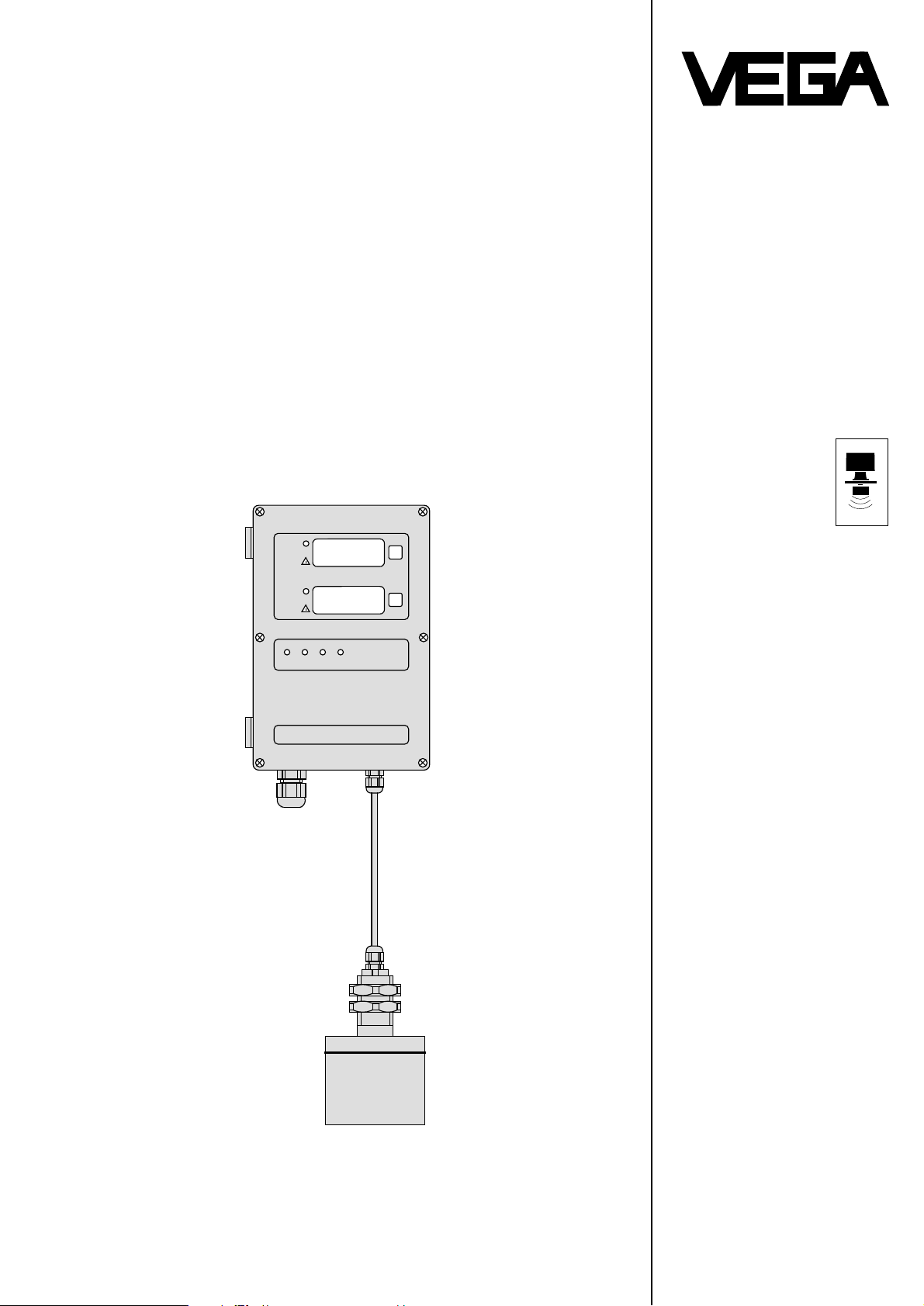
VEGASON 71 - D

TIB • Technical Information • Operating Instructions

Pulse-echo measuring system

1 2

1 2 3

5.000

VEGASON

Single channel flow measurement

Approvals for hazardous areas, certificate acc. to CENELEC

VEGA Grieshaber KG

Am Hohenstein 113 D-77761 Schiltach Phone 0 78 36 / 50 - 0 Fax 0 78 36 / 50 201

Contents

1 Introduction

1.1 Contents of the instruction manual .....................................................................................................................4

1.2 Safety information ...............................................................................................................................................4

1.3 Product description .............................................................................................................................................4

1.4 Approvals ............................................................................................................................................................4

2 Technical Information

2.1 Configuration of a measuring system .................................................................................................................5

2.2 Technical data, VEGASON 71 - D.......................................................................................................................6

2.3 Technical data, transducer ..................................................................................................................................7

2.3 Dimensional drawings ......................................................................................................................................... 8

2.4 Measuring range .................................................................................................................................................8

2.5 General installation instructions ..........................................................................................................................9

2.6 Installation fault .................................................................................................................................................10

2.7 Electrical connection ......................................................................................................................................... 11

Contents

3 Operating surface

3.1 Indicating and operating elements ....................................................................................................................12

3.2 Operation .......................................................................................................................................................... 13

4 Set-up

4.1 Flow chart for set-up ......................................................................................................................................... 14

4.2 Mode range, general parameter adjustment, mode 0 - 00 … 0 - 99 ................................................................. 15

5 Adjustment

5.1 Empty / full adjustment in metres without flow change ..................................................................................... 18

5.2 Demonstration and programming example .......................................................................................................18

6 Flow measurement

6.1 Linearization......................................................................................................................................................19

6.1.1 Meter flume / weir .................................................................................................................................. 19

6.1.2 Enquiry of linearization curves 4 … 6 ....................................................................................................20

6.2 Linearity protocol...............................................................................................................................................22

VEGASON 71 - D

Contents

7 Output results

7.1 Display ..............................................................................................................................................................23

7.1.1 Allocation of a multiplication factor.........................................................................................................23

7.1.2 Measuring unit .......................................................................................................................................23

7.1.3 Decimal point .........................................................................................................................................23

7.1.4 Integration time ......................................................................................................................................24

7.2 Adjustment max. flow ........................................................................................................................................24

7.3 Impulse value for flow relay ...............................................................................................................................24

7.4 Impulse value for sampling relay.......................................................................................................................24

7.5 Definition of the min. flow volume limit ..............................................................................................................25

7.6 Calculation examples of the max. flow ..............................................................................................................25

7.6.1 Khafagi-Venturi flume.............................................................................................................................26

7.6.2 Trapezoidal weir (Cipolletti) ....................................................................................................................27

7.6.3 Rectangular weir without throat .............................................................................................................28

7.6.4 Rectangular weir with throat ..................................................................................................................29

7.6.5 V-Notch .................................................................................................................................................. 30

7.6.6 Palmer-Bowlus-flume .............................................................................................................................31

7.7 Level module.....................................................................................................................................................32

7.7.1 Coordinations and their relations ...........................................................................................................32

7.7.2 Switching commands .............................................................................................................................32

7.8 Current module .................................................................................................................................................33

8 Supplementary programmings

8.1 Failure processing............................................................................................................................................. 33

8.2 Simulation .........................................................................................................................................................34

8.3 Basic adjustment, mode range general parameter adjustment.........................................................................34

8.4 Keyword ............................................................................................................................................................ 34

9 Optimization

9.1 Enquiry of the optimization................................................................................................................................35

9.2 Mode range optimization, mode 1 - 01 … 1 - 27...............................................................................................36

9.3 Definition of the operating range .......................................................................................................................37

9.4 Multiple echo reduction .....................................................................................................................................37

9.5 Adjustment of the max. gain .............................................................................................................................37

9.6 Fault signal........................................................................................................................................................ 38

9.8 Protocol of the optimization...............................................................................................................................38

9.7 Basic adjustment, mode range optimization .....................................................................................................38

10 Supplement

10.1 Error codes........................................................................................................................................................39

10.2 Error schedule...................................................................................................................................................39

VEGASON 71 - D

1 Introduction

1.1 Contents of the instruction manual

The Technical Information / Operating Instructions is called TIB. It contains all necessary information for correct

- installation

- connection

- set-up

- linearization

- optimization of the pulse-echo-measuring system VEGASON 71 - D.

VEGA regularly revises the contents of TIBs as technical improvements are made to the instruments.

1.2 Safety information

The described module must only be installed and operated as described in this TIB. Please note that other action can cause damage for which VEGA does not accept responsiblity.

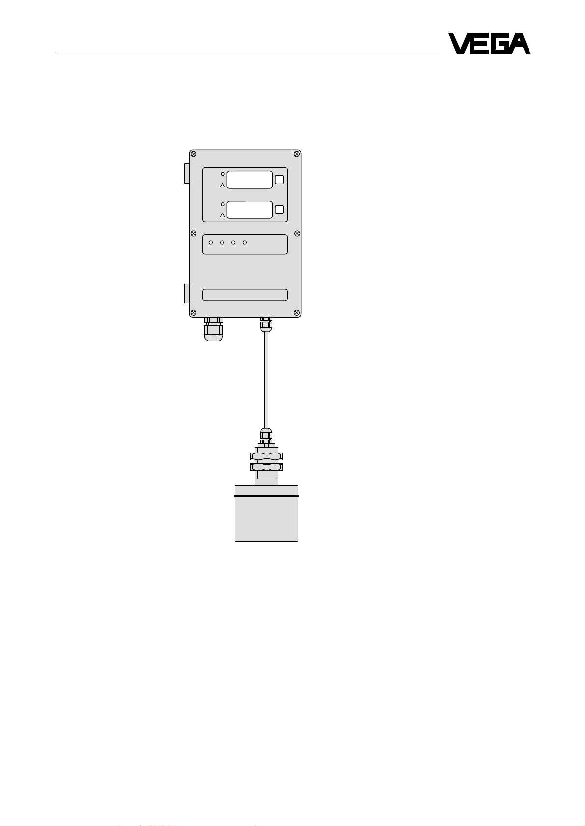
1.3 Product description

The pulse-echo measuring system VEGASON 71 - D is used for flow and level measurement.

A measuring system consists of

- a central electronics and

- a sensor. The sensor is provided with a temperature sensor for

compensation of the temperature influence to the sound running period. Measuring data and temperature information are transmitted along the same coaxial cable.

All adjustment procedures, optimizations etc. can be directly programmed via a keyboard on the central electronics.

1.4 Approvals

If a measuring system is mounted acc. to the following approval, the respective legal document has to be used and the regulations have to be strictly observed.

Approvals for hazardous areas, certificate acc. to CENELEC.

Consisting of:

- central electronics VEGASON 71 - D

- sensor SW 71 R Ex defined in the conformity certificate PTB-no. Ex-94.C.4066.

The running periods of periodically emitted sound impulse packets which are reflected by the flow product to be measured are evaluated.

The running period of sound is a measure of the distance between sensor and liquid surface.

The control electronics determines this distance and converts it into flow information.

The measuring results are indicated on the integral LCdisplay and acc. to the version, provided as relay and current outputs.

The conformity certificate is included with the product on delivery.

VEGASON 71 - D

2 Technical Information

2.1 Configuration of a measuring system

Input Central electronics Outputs

Measuring data from the sensor 2 LC-display (multi-functional indication)

5.000

1 2

1 2 3

VEGASON

Flow module

- 1 relay output for flow

- 1 relay output for sampling Level module

- 2 relay outputs Current module

- 1 output flow proportional module

- 1 output level proportional module

Sensor

Central electronics consisting of:

- plastic housing with cover

- operating elements (5 keys)

- LED-display

- two LC-displays (multi-functional displays)

- power supply unit

- data memory (EEPROM, no buffer battery required)

- outputs: flow module, level module, current module

- terminals for power supply, inputs and outputs

VEGASON 71 - D

Sensor:

- in standard version or

- in Ex-version, certificate acc. to CENELEC Accessories:

- swivelling holder for sensor mounting Options:

- totalising counter (flow)

- indicator VEGADIS 171 A

- overvoltage arresters

2.2 T echnical data, VEGASON 71 - D

Power supply

Operating voltage

- Standard U

- Option U Power consumption at U Fuse for version

and max-load 12 V A, 5 W

nenn

16 … 42 V AC or 16 … 60 V DC 2 A 90 … 250 V AC 500 mA

Measuring range

Min. distance 0.300 m Max. distance 4.000 m (5.000 m)

Measuring data

Min. span 10 cm Display in m (0.000 … 5.000 distance) Resolution in mm Scanning 3 mm Measuring frequency 50 kHz Measuring rate 0,4 sec. Angle of reflection (at –3 dB) 8° Linearity error after empty and full adjustment < 0,1 % of measuring range Temperature error of the electronics 0,1 % / 10 k of measuring range

= 24 V AC (16 … 42 V), 50/60 Hz

nenn

= 24 V DC (16 … 60 V)

nenn

= 230 V AC (90 … 250 V), 50/60 Hz

nenn

2 T echnical Information

Central electronics

Inputs 1 (1 channel, for 1 sensor) Outputs see section "output" Housing material Polycarbonate Electrical connection max. 1,5 mm

Cable entry 1 x Pg 7, 1 x Pg 13,5 (up to max. 5 x Pg 13,5) Protection IP 65 Ambient temperature -20°C … +60°C Storage and transport temperature -20°C … +80°C Weight approx. 1,9 kg

Output Indication

LC-display 2, 4-digit each

Flow module

1 flow relay output active, with status indication (LED)

- voltage impulse 24 V

- current impulse 20 mA

- pulse duration 200 ms 1 sampling relay output floating spdt, with status indication (LED)

- contact material AgCdO and Au plated

- min. turn-on voltage 10 mV switching current 10 µA

- max. turn-on voltage 250 V AC, 60 V DC switching current 2 A AC, 1 A DC

- max. breaking capacity 125 V A, 60 W

VEGASON 71 - D

2 Technical Information

Level module

2 relay outputs floating spdts each

and 2 status indications (LEDs)

- contact material AgCdO and Au plated

- min. turn-on voltage 10 mV switching current 10 µA

- max. turn-on voltage 250 V AC, 60 V DC switching current 2 A AC, 1 A DC

- max. breaking capacity 125 V A, 60 W

Current module

2 current outputs

- range 0/4 … 20 mA

- resolution 0,05 % of range

- load max. 500 Ohm

- load dependent error at 0 … 500 Ohm, < 0,2 % related to the range

or module as described above however with 2 floating outputs each

Fault signal

1 fail safe relay 1 floating spdt contact data as described under relay outputs 2 failure-LEDs

2.3 Technical data, transducer

Transducer SW 71

Material of the transducer housing PVDF Material of the fixing tube PVDF, thread G 1 A Connection cable to central electronics standard coaxial cable type RG 58 Cable length 5 m, as option 300 m Diameter of cable approx. 5 mm Temperature sensor integrated in the transducer Ambient temperature -20°C … +80°C Storage and transport pressure -20°C … +80°C Protection IP 68 Permissible ambient temperature 1 bar Weight approx. 0,8 kg

Transducer SW 71 R Ex

Ex-approval PTB-no. Ex-94.C.4066 Flame proofing Casting "m" Marking EEx m II T6 or T5 or T4 Material of the transducer housing PVDF Material of the fixing tube PVDF, thread G 1 A Connection cable to central electronics standard coaxial cable type RG 58 Cable length 5 m, as option up to 300 m Diameter of cable approx. 5 mm Temperature sensor integrated in the transducer Temperature class T6 = 60°C, T5 = 75°C, T4 = 80°C Storage and transport temperature -20°C … +80°C Protection IP 68 Permissible ambient pressure 1 bar Weight approx. 1,0 kg

VEGASON 71 - D

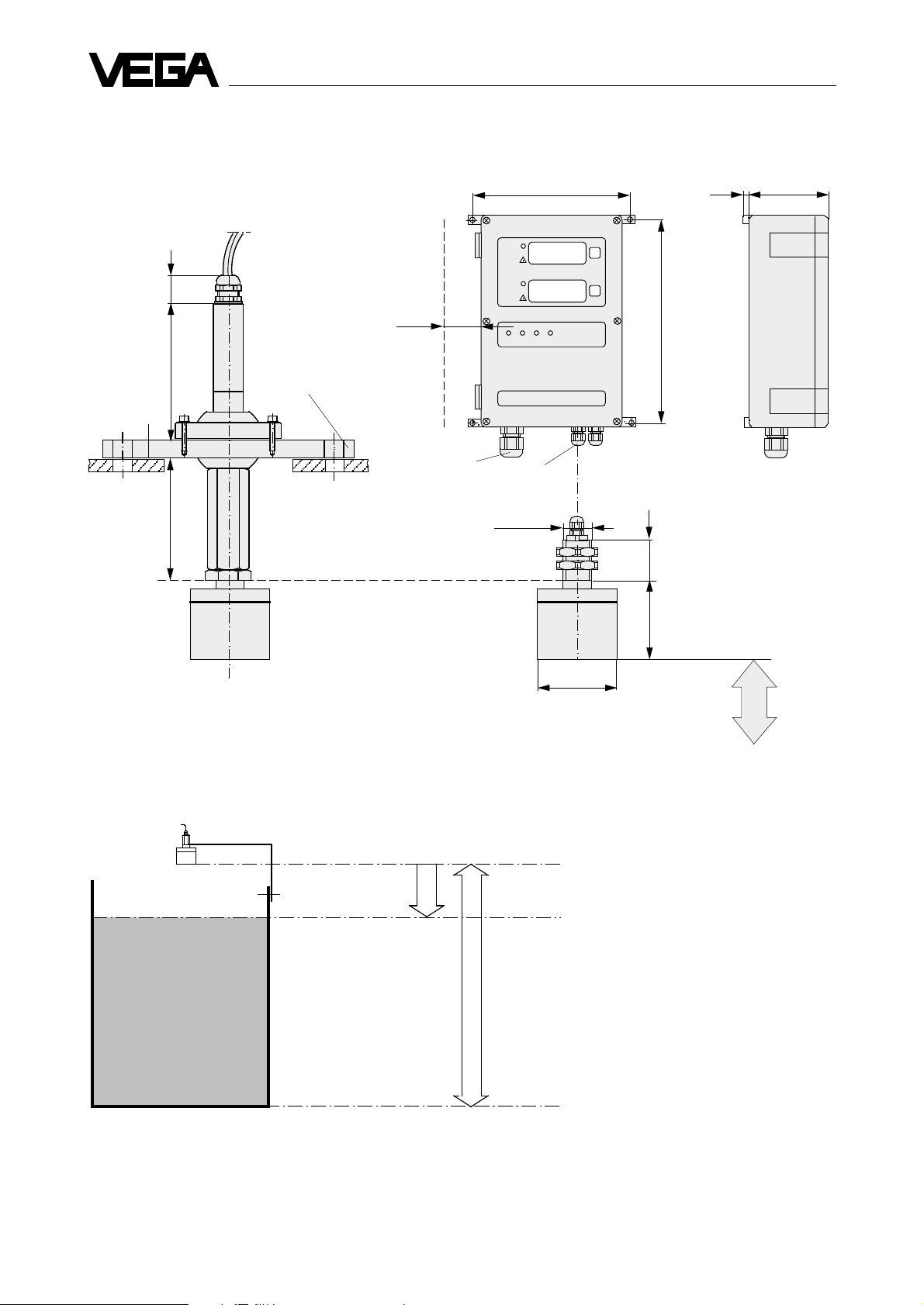
2.3 Dimensional drawings

(Dimensions in mm)

2 T echnical Information

Swivelling flange

138

Central electronics

Min. distance for adjacent instrument

Flange DN 150 PN 16

1 2

1 2 3

Pg 13,5 Pg 7

G 1 A

Sensor

*174

VEGASON

*229

* Mounting diemsnions

2.4 Measuring range

Reference plane

Min.-distance

Measuring range

ø95

Min.-distance

300 mm

0.000 m

0.300 m

max.

4.000 m (5.000 m)

VEGASON 71 - D

2 Technical Information

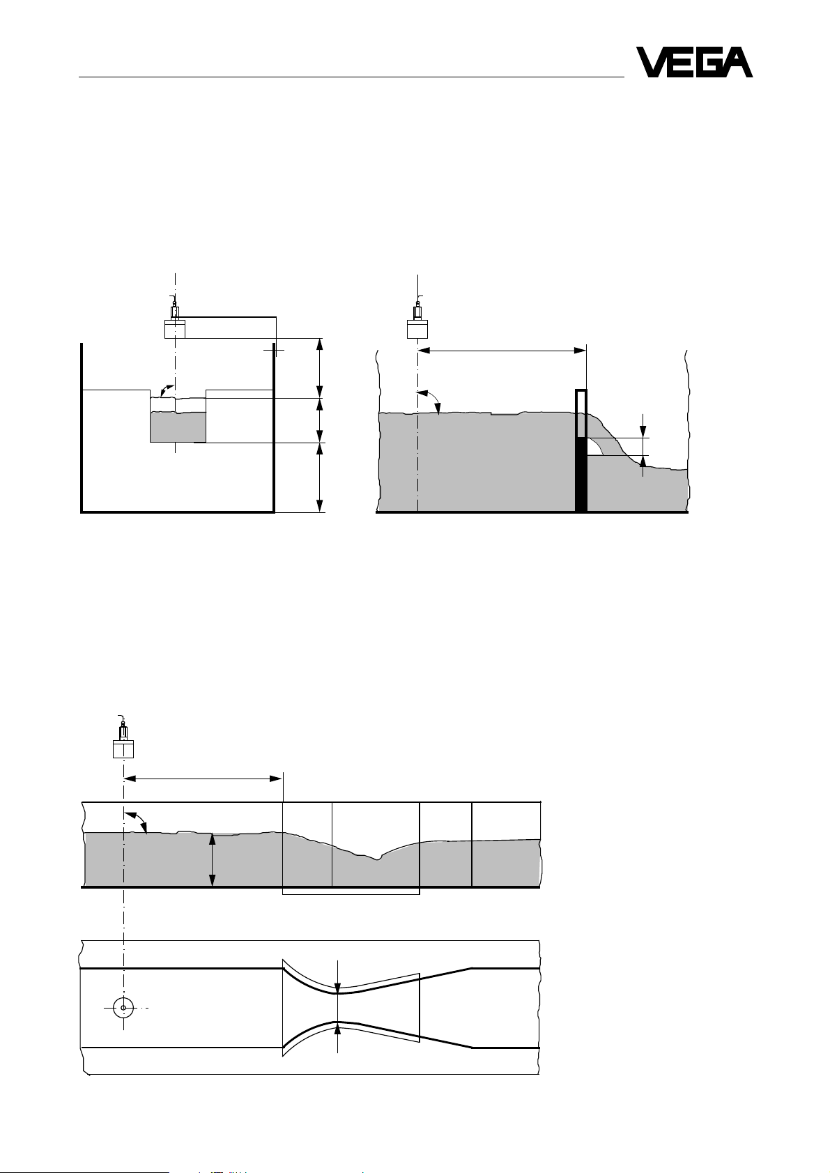
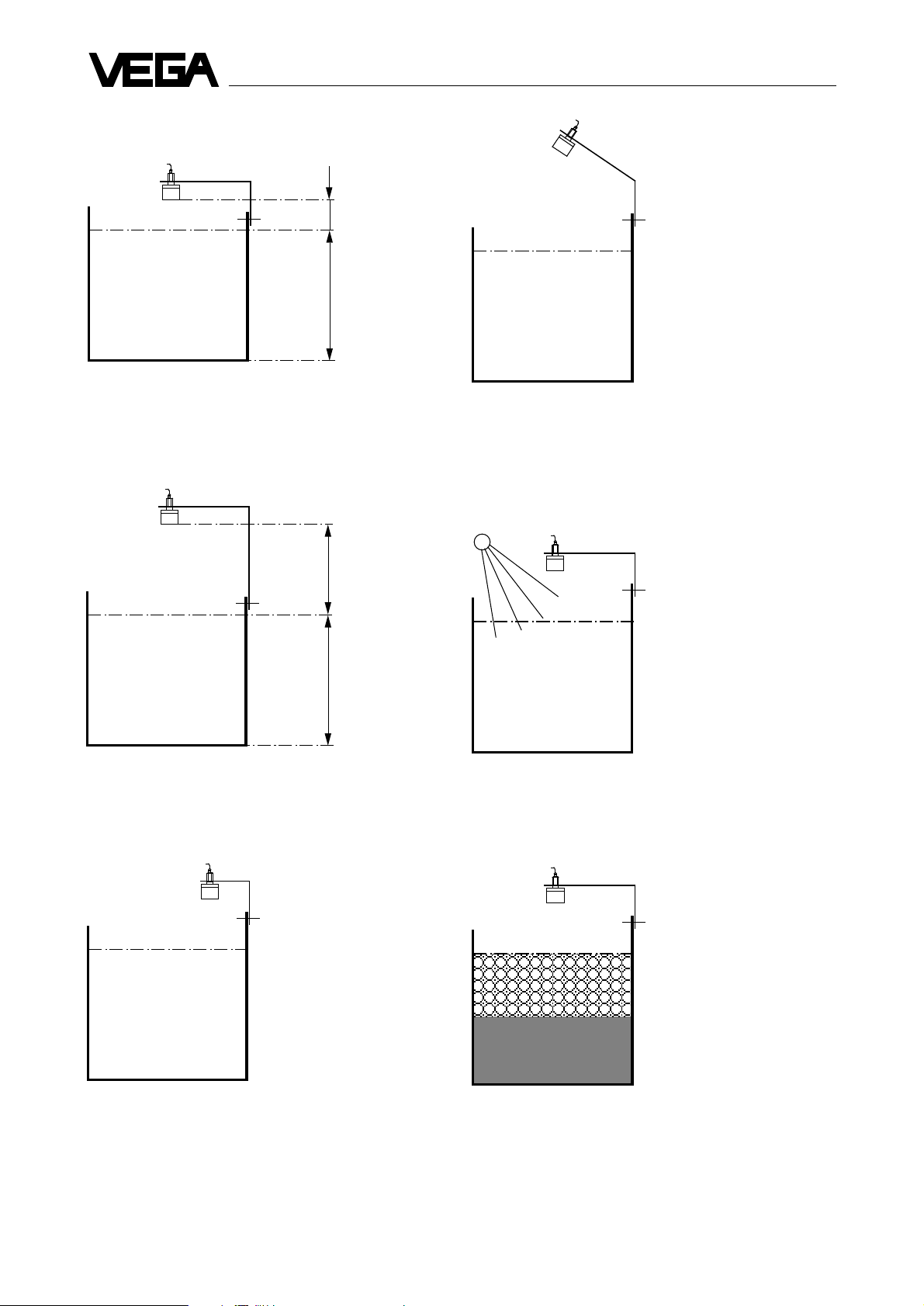
2.5 General installation instructions

Open flume with weir (e.g. rectangular)

- Installation of the transducer upstream

- Observe distance to the weir (3 … 4 x h

- Installation if possible centered to the flume

- Installation vertical to the surface of the flow product

- Observe min. distance relating to h

- Min. distance diaphragm opening to downstream water ≥ 5 cm

90°

weir

max

)

≥ Min.-

max

≥ 2 x h

distance

3 - 4 x h

max

90°

upstream water

≥ 5 cm

downstream water

Open flume with measuring channel (e.g. Khafagi-Venturi flume)

- Installation of the sensor at the inlet

- Observe distance to the Khafagi-Venturi flume (3…4xh

- Installation if possible centered to the flume

- Installation vertically to the surface of the flow product

- Min. distance relating to the height of damping h

max

Note

Otherwise follow the installation guidelines given by the channel manufacturer.

Sensor

3 - 4 x h

max

90°

max

)

Sensor

VEGASON 71 - D

2.6 Installation fault

< 300 mm

max

2 T echnical Information

Fault: Min. distance from sensor to h

maintained.

max

not

Problem: The upper range cannot be measured. Solution: Correct min. distance of the sensor to 0,3 m.

> 300 mm

max

Fault: Distance from sensor to h Problem: Unreliable results due to very weak echoes.

too large.

max

Solution: Correct min. distance of the sensor to 0,3 m.

Fault: Sensor is not directed vertically to the surface. Problem: Sensor receives weak echoes. Solution: Mount sensor vertically.

Fault: Strong heat fluctuations, e.g. sun. Problem: The measuring accuracy is not constant. Solution: Install a sun shield in the respective position.

Fault: Sensor too close to the flume wall, i.e. not

mounted in the centre.

Problem: Build-up and rough flume walls cause

measuring problems.

Solution: Mount sensor in the centre of the flume.

Fault: Surface has foaming problem. Problem: The surface of the foam is detected as level.

The measured value is wrong.

Solution: The used measuring principle is not suitable

and must be replaced e.g. by a hydrostatic system (pressure transmitter).

VEGASON 71 - D

2 Technical Information

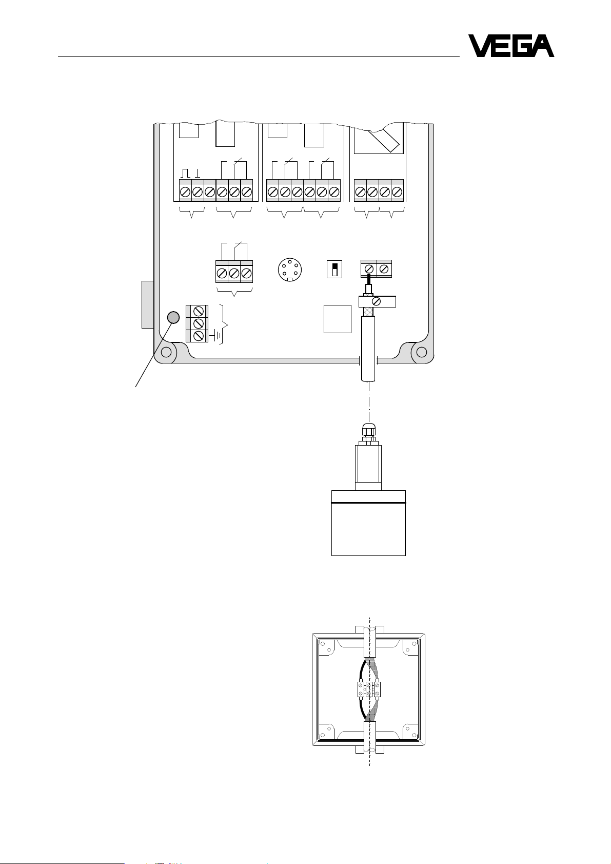
2.7 Electrical connection

Flow module

Flow module:

- Flow Terminal 9 and 10

- Sampling Terminal 12 … 14

91011

Relay output

Fuse type TR5 Manufacturer, e.g. Messrs. Wickmann, Current value see 2.2 Technical Data

1 2

13 14

Service socket

Failure relay output

Power supply

Level module

15 16

1 2

Relay output

Service switch

1 2

Attention!

High

voltage

Current module

+ - + -

21 22

1 2

Current output

standard coax cable max. cable length = 300 mm

Current module:

- flow proportional Terminal 21 and 22

- level proportional Terminal 23 and 24

Note

During operation the sensor is clocked with highperformance impulses. It is therefore recommended to provide all electrical connections first and then switch on the power supply.

The connection line to the sensor can be extended as shown. Therefore observe that a max. line length of 300 m is not be exceeded.

Sensor

standard waterproof distributor box

VEGASON 71 - D

3 Operating surface

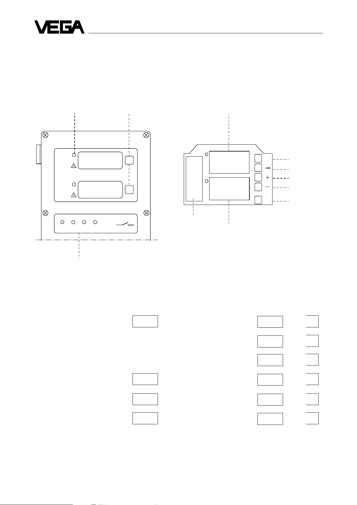
3.1 Indicating and operating elements

Outer view Inner view

3 Operating surface

LED-indication Fault signal

8888

1 2 3

LED-indication of the relay output 1 … 4

Measuring units as label in the provided window

Scheme of operation

Indication of measured values MODEFIELD

8888

PARAMETER FIELD

MOD

STO

Selection of mode

Cursor position figures raise figures lower

Memory

Indication of measured values

e.g. flow 00.00 … 75.00 11.25 m3/h

Demonstration after respective programming of

- Measuring unit

- Allocation of a multiplication factor

- Decimal point e.g. Flow 0 … 100 % 50.0 %

Level 0 … 100 % 50.00 %

Distance 0.000 … 5.000 m 5.000 m

Mode range

General parameter adjustment 0 - 00 … 99

Optimization 1 - 01 … 27

Linearization curve 4 4.H.01 … 32

Linearization curve 5 5.H.01 … 32

Linearization curve 6 6.H.01 … 32

Fault signals E2.01 … .04

VEGASON 71 - D

3 Operating surface

3.2 Operation

VEGASON 71 - D has 3 modes which can be enquired with the MOD-button (scrolling)

- indication of measured values

- mode range

- parameter adjustment. After 60 mins. VEGASON 71 - D resets automatically to mode "Indication of measured values".

1. Indication

of measured values

2. Mode

range

3. Parameter

adjustment

5.000

MOD

0Ê00 0Ê99

48.94

MOD

Cursor position Figures raise Figures lower

0 - 00

– – – – 0

Cursor position

MOD

Figures raise Figures lower

STO

1. Indication of measured value Flow in m

/h Flow in % Level in % Distance in m

2. Mode range Enquiry of the mode numbers in the MODEFIELD. The parameters of the enquired mode numbers can be checked or modified in mode 3.

3. Parameter adjustment Programming of the parameters in the PARAMETER FIELD. The parameter of the respectively enquired mode can be modified and stored with the key STO. Push the MOD-key if no modification is desired or if the modified parameter should not be stored. In both cases reset in mode 1.

In mode 99 the mode range of the general parameter adjustment can be quit and the optimization as well as the linearization curve 4 … 6 can be enquired. Reset also in mode 99.

If after STO the actual mode range is enquired again within 60 mins., the last enquired mode number appears automatically.

VEGASON 71 - D

4 Set-up

4.1 Flow chart for set-up

Connect sensor to control electronics and switch on the power supply .

4 Set-up

The software version is displayed and the fault signal responds.

The measuring system is ready and starts the self-check cycle. Preliminary indication:

0.000 m

Self-check cycle, i.e.:

1. Echo limitation from top to bottom.

2. Echo limitation from bottom to top.

3. Generation of a measuring window, within which a preferred processing of the echo is made.

Feeding

phase:

5 6

Sensor

Flume

48.94

0.000 m

Echo

Measuring window

After approx. 1 … 3 min. the measuring system is in operating status. The fault signal extinguishes. The measuring system has finished the self-check and operates with the parameters of the factory setting.

YES

Flow measurement

(level measurement in flume)

5 6

Optimization required.

In the flume a distance of e.g. 0,600 m is determined.

0.600 m

VEGASON 71 - D

4 Set-up

4.2 Mode range, general parameter adjustment, mode

0 - 000 - 00

0 - 00 …

0 - 000 - 00

0 - 990 - 99

0 - 99

0 - 990 - 99

Function Mode-no. Mode description Parameter Page

(bold = factory setting)

0 - 00 Software version .................................................... z.B. 48.94

0 - 01 … 10 not coordinated ...................................................... ––––

Adjustment 0 - 11 Empty adjustment

- distance in m ..................................................... 5.000 m … 0.000 m

- level in % ...........................................................

0.00.0

0.0 … 80.0 P. 18

0.00.0

0 - 12 Full adjustment

- distance in m ..................................................... 0.000 m … 5.000 m

- level in % ...........................................................

100.0100.0

100.0 … 20.0

100.0100.0

Display Allocation of a multiplication factor

function 0 - 13 - relating to 0 % ...................................................

0 - 14 - relating to 100 % ............................................... 0000 …

00000000

0000 … 9999

00000000

10001000

1000 … 9999

10001000

0 - 15 Measuring unit P. 23

- distance in m .....................................................

- level in % ........................................................... 2

- scaled value ...................................................... 3

0 - 16 Decimal point ......................................................... 0.000 …

0 - 17 Integration time ......................................................

0 … 900 P. 24

000.0 000.0

000.0 … 0000

000.0 000.0

Lineari- 0 - 18 Linearization curves

zation - linear ................................................................. 1

- not coordinated ................................................. 2

- not coordinated ................................................. 3

- individually programmable curve 4 .................... 4

- individually programmable curve 5 .................... 5

- individually programmable curve 6 .................... 6

- root function Q = K x h

- linear function Q = K x h

0,5

................................... 7

1,0

.................................

- Venturi flume rectangular flume rectangular weir trapezoidal weir Q = K x h

- Palmer Bowlus Flume Q = K x h

- quadratic function Q = K x h

- V-Notch Q = K x h

2,5

........................................................ 12

1,5

.............................. 9

1,86

................... 10

2,0

................................................

0 - 19 … 52 not coordinated ...................................................... ––––

Level 0 - 53 Coordination

module - measuring result in m ........................................ 1

Relay output 1

0 - 54 not coordinated ...................................................... –––– P. 32

- measuring result in %........................................

Switching command

0 - 55 - on ...................................................................... 0.000 m … 5.000 m

0 - 56 - off ...................................................................... 0.000 m … 5.000 m

8 P. 20

VEGASON 71 - D

0 - 57 not coordinated ...................................................... ––––

4 Set-up

4.2 Mode range, general parameter adjustment (continuation)

Function Mode-no. Mode description Parameter Page

(bold = factory settings)

(level 0 - 58 Coordination

module) - measuring result in m........................................ 1

Relay output 2

Current Characteristics

module 0 - 65 - end ....................................................................

Current output 1 + 2

0 - 59 not coordinated ...................................................... –––– P. 32

0 - 60 - on ...................................................................... 0.000 m … 5.000 m

0 - 61 - off ...................................................................... 0.000 m … 5.000 m

0 - 62 … 64 not coordinated ...................................................... ––––

0 - 66 - begin ................................................................. 00.00 …

0 - 67 … 81 not coordinated ...................................................... ––––

- measuring result in %........................................

Switching command

20.0020.00

20.00 … 00.00 P. 33

20.0020.00

04.0004.00

04.00 … 20.00

04.0004.00

Max. 0 - 82 Flow (max. 4 positions) .......................................... 0001 … 9999 …

flow 0 - 83 Multiplier

(at level - flow x 1 ..............................................................

100 %) - flow x 10 ............................................................ 1

- flow x 100 .......................................................... 2 P. 24

- flow x 1000 ........................................................ 3

0 - 84 Time unit for above flow

- seconds .............................................................

- minutes.............................................................. 2

- hours ................................................................. 3

Flow module

Pulse value 0 - 85 Flow quantity / impulse .......................................... 0001 … 9999 …

for flow 0 - 86 Multiplier

relay - flow quantity / impulse x 1 .................................

- flow quantity / impulse x 10 ............................... 1

- flow quantity / impulse x 100 ............................. 2

- flow quantity / impulse x 1000 ........................... 3

Pulse value 0 - 87 Flow quantity / impulse .......................................... 0001 … 9999 …

for samp- 0 - 88 Multiplier

ling relay - flow quantity / impulse x 1 ................................. 0

- flow quantity / impulse x 10 ...............................

- flow quantity / impulse x 100 ............................. 2 P. 25

- flow quantity / impulse x 1000 ........................... 3

- flow quantity / impulse x 10000 ......................... 4

- flow quantity / impulse x 100000 ....................... 5

- flow quantity / impulse x 1000000 ..................... 6

0 P. 24

10001000

1000

10001000

1000

10001000

1000

10001000

0 - 89 Time dependent controls in hours .........................

0 - 90 Min. flow volume limit in % .....................................

0 - 91 u. 92 not coordinated ...................................................... ––––

0 (off) … 100

0.00.0

0.0 … 100 P. 25

0.00.0

VEGASON 71 - D

4 Set-up

4.2 Mode range, general parameter adjustment (continuation)

Function Mode-no. Mode description Parameter Page

(bold = factory settings)

0 - 93 Failure processing

- store actual current,

switching relay unchanged ................................

- current 0 mA, switching relay de-energized ...... 2 P. 33

- current corresponds to 0 %,

switching relay de-energized ............................. 3

- current corresponds to 100 %,

switching relay de-energized ............................. 4

0 - 94 Simulation .............................................................. 0.000 m … 9.999 m P. 34

0 - 95 u. 96 not coordinated ...................................................... ––––

0 - 97 Basic adjustment

- switched off .......................................................

- switched on ....................................................... 1

0 - 98 Keyword (= 0070)

- switched off .......................................................

- switched on ....................................................... 1

0 P. 34

0 - 99 Change

- general parameter adjustment ..........................

- optimization ....................................................... 1 P. 20

- not coordinated ................................................. 2 and

- linearization curve 4 .......................................... 4 P. 35

- lineariztion curve 5 ............................................ 5

- linearization curve 6 .......................................... 6

VEGASON 71 - D

5 Adjustment

5.1 Empty / full adjustment in metres without flow change

With this adjustment procedure two distances in m are defined which correspond to the levels of 0 % and 100 %.

5.2 Demonstration and programming example

Demonstration

m %

0.000

0.350

0.700

100

0.35 m distance ^ 100 %

0.7 m distance ^0%

Programming example

0.350 m distance ^ 100 %

• Enquire mode 0 - 12 in the MODEFIELD

• Program 0.350 m in the PARAMETER FIELD

• Then store with key STO

0.700 m distance ^ 0 %

• Enquire mode 0 - 11 in the MODEFIELD

• Program 0.700 m in the PARAMETER FIELD

• Then store with key STO (The sequence of the empty and full adjustment is individual)

VEGASON 71 - D

6 Flow measurement

6.1 Linearization

6.1.1 Meter flume / weir

The system measures the level and calculates the flow. The relationship between level and flow is linear in most

cases. The level value (in %) must be therefore converted into a

flow porportional value. The necessary mathematical functions depend on the

flumes and weirs used. For the standard flumes and weirs the respective functions

are available as pre-programmed linearization curves and can be directly enquired.

Flumes / weirs which do not correspond to the known functions, can be imitated via three programmable linearization curves.

Standard flumes / weirs

Pre-programmed linearization curves

Enquire linearization curves

0 - 18 = 1

bis

NO standard flumes / weirs

Programmable linearization curves

Enquire mode range

0 - 99 = 4

5 6

Program index markers for linearization curves

4 - 01 … 32 5 - 01 … 32 6 - 01 … 32

Enquire linearization curves

0 - 18 = 4

5 6

Processing results flow proportional

VEGASON 71 - D

6 Flow measurement

6.1 Linearization (continuation)

6.1.2 Enquiry of linearization curves 4 … 6

In mode 0 - 99 linearization curves 4 … 6 can be enquired as well as the reset (mode 4 - 99, 5 - 99, 6 - 99) to the general parameter adjustment can be made.

0 - 9 9

5 H . 0 1

4 H . 0 1

Enquiry linearization curve 4 … 6

Reset to general parameter adjustment

0 - 0 1

Programming example

Linearization curve 4

• Enquire mode 0 - 99 in the MODEFIELD

• Program figure 4 in the PARAMETER FIELD

• Then store with STO

• Push MOD-key for enquiry of the index markers Reset is always made in mode 99 with figure 0 in the P ARAMETER FIELD.

Linearization curve 4

6 H . 0 1

4 - 9 9

Function Mode-no. Mode description Parameter

(bold = factory setting)

Index 4.H.01 1. index markers - level percent ................... 000.0 …

markers 4.L.01 - flow percent .................... 000.0 …

bis to

4.H.32 32. index markers - level percent ................... 000.0 …

4.L.32 - flow percent .................... 000.0 …

4 - 33 … 98 not coordinated .................................................... ––––

4 - 99 Change

- general parameter adjustment......................... 0

- optimization ..................................................... 1

- not coordinated ................................................ 2

- linearization curve 4 ........................................ 4

- linearization curve 5 ........................................ 5

- linearization curve 6 ........................................ 6

Linearization curve 5 as linearization curve 4, however 5.H.01 … 5.H.32

5.L.01 … 5.L.32 5 and 5 - 99

Linearization curve 6 as linearization curve 4, however 6.H.01 … 6.H.32

6.L.01 … 6.L.32 6 and 6 - 99

100.0100.0

100.0

100.0100.0

100.0

100.0100.0

100.0

100.0100.0

100.0

100.0100.0

VEGASON 71 - D

6 Flow measurement

Display

4 = no. of the linearization curve

Change-over

Display 1

Display 2

Display 1

Display 2

H H

4 .

H . 0 1

H H

1 0 0 . 0

L L

4 .

L . 0 1

L L

1 0 0 . 0

H = indication for level percent 01 = 1. index markers

MODEFIELD

P ARAMETER FIELD

level percent value (factory setting)

L = indication for flow percent 01 = 1. index markers

MODEFIELD

PARAMETER FIELD

flow percent value (factory setting)

4 .

0 1

4 .

9 1

4 .

H H

H . 0 1

H H

L L

L . 0 1

L L

Example of a linearization curve

Flow

%

4.L.05

100.0



100

4 .

4 . L

. 0

scrolling with key –>

scrolling with key + or –

Example of a linearity protocol

Index marker Level percent Flow percent no. (level)

01 30.0 % 10.0 % 02 50.0 % 15.0 % 03 75.0 % 40.0 % 04 90.0 % 70.0 % 05 100.0 % 100.0 %

4.L.01

010.0

VEGASON 71 - D

Level

50 100 %

4.H.01

030.0

4.H.05

100.0

6 Flow measurement

6.1 Linearization (continuation)

Programming example

When programming the level and flow percent values, observe the following:

- The starting point of the characteristics (index marker

00) is generated by the instrument itself and coordinated with the values H = 0.0, L = 0.0.

- The end (last index marker) can be made individually within the 32 value pairs.

- The last index marker must only consist of 100.0 level percent and 100.0 flow percent.

Programming acc. to linearity protocol

(see e.g. page 21)

Index marker 01 (level percent)

• Enquire index marker 4.H.01 in the MODEFIELD

• Program 30 % in the PARAMETER FIELD acc. to the linearization curve

• Then store with STO

Index marker 01 (flow percent)

• Enquire index marker 4.L.01 in the MODEFIELD

• Program 10 % in the PARAMETER FIELD acc. to the linearization curve

• Then store with STO

etc. acc. to linearity protocol. After programming of all data

- reset to mode range 0

- change display indication to flow proportional indication, i.e. mode 0 - 13 … 0 - 16

- here in the example activate the programmed linearization curve, i.e. mode 0 - 18 = 4.

6.2 Linearity protocol

Linearization curve

Index Level percent Flow percent marker no. (level)

01 02 03 04 05 06 07 08 09 10 11 12 13 14 15 16 17 18 19 20 21 22 23 24 25 26 27 28 29 30 31 32 Date Name

VEGASON 71 - D

7 Output results

7.1 Display

7.1.1 Allocation of a multiplication factor

If an indication in flow m3/h is requested, first an allocation of a multiplication factor to the measured level 0 % and 100 % must be carried out in mode 0 - 13 and 0 - 14.

This allocation of a multiplication factor is only valid for the indication and does not influence the output results for the relay and current outputs.

7.1.2 Measuring unit

In mode 0 - 15 first of all the level proportional indication is converted to a linearized, flow percentage indication, derived from the allocation of a multiplication factor.

Furthermore different measuring units can be inserted as label into the respective window.

7.1.3 Decimal point

Furthermore the position of the decimal point can be determined in mode 0 - 16.

Programming example

Allocation of a multiplier for 0 %

• Enquire mode 0 - 13 in the MODEFIELD

• Program the figure 0000 in the P ARAMETER FIELD

• Then store with STO On display 1 the actual distance of 0.525 m is indicated at

the moment.

Allocation of a multiplier for 100 %

• Enquire mode 0 - 14 in the MODEFIELD

• Program the figure 7500 in the PARAMETER FIELD

• Then store with STO On display 1 still the actual distance of 0.525 m is

indicated.

Measuring unit and label

• Enquire mode 0 - 15 in the MODEFIELD

• Program the figure 3 in the PARAMETER FIELD

• Then store with STO On the display 15 % (linearized value) of the previously

programmed allocation of a multiplier are indicated (112.5).

Demonstration to the programming example

- adjustment see page 18

- linearization curve, page 21

Mode

0-15 = 1 0-15 = 2 0-15 = 3 distance level flow in m in % in %

0.350

0.525

0.700

100

15 0

Position of the decimal point

• Enquire mode 0 - 16 in the MODEFIELD

• Shift with key –> the position of the decimal point to the right until the requested position is reached

• Then store with STO

The desired form is indicated on the display (11.25). Insert the label m

Flow acc. to allocation of a multiplier in m

0 - 14

= 75.00

= 00.00

0 - 13

/h into the window.

11.25

VEGASON 71 - D

7 Output results

7.1.4 Integration time

An integration time can be programmed in mode 0 - 17 to damp probable fluctuations during the indication of measured values.

Programming example

Integration time = 10 secs.

• Enquire mode 0 - 17 in the MODEFIELD

• Program figure 010 in the PARAMETER FIELD

• Then store with STO

7.2 Adjustment max. flow

The adjustment of the max. flow at 100 % is necessary to enable the conversion of flow to flow volume.

The value given by the manufacturer of the weir or flume at max. flow must be adjusted (this value must be reached at 100 % of the adjustment carried out).

If the weir of flume is oversized or the data for max. flow are not known, the required adjustment parameters can be determined as described in chapter "7.6 Calculation examples of the max. flow".

7.3 Impulse value for flow relay

It is possible to connect a counter to VEGASON 71 - D to detect the flow quantity. When using a 24 V counter, it can be directly connected to the flow module, terminal 9 and

10.

In mode 0 - 85 and 0 - 86 the multiplier of the step-down ratio (flow volume/pulse) can be determined.

Note

The instrument automatically takes the measuring unit selected for the adjustment of the max. flow.

Example

One impulse on the counter per 5 m corresponds to 0005 x 1 m

- Mode 0 - 85, flow volume / impulse = 0005

- Mode 0 - 86, multiplier = 0

Programming

Flow volume / impulse = 0005

• Enquire mode 0 - 85 in the MODEFIELD

• Program figure 0005 in the PARAMETER FIELD

• Then store with STO

Note

The adjusted measuring unit is also valid for the following programmings of the pulse rate.

Example

Max. flow acc. to manufacturers data = 364 m3/h corresponds to 0364 x 1 m

- Mode 0 - 82, flow = 0364

- Mode 0 - 83, multiplier = 0

- Mode 0 - 84, time unit = 3 (h)

Programming

Flow = 364

• Enquire mode 0 - 82 in the MODEFIELD

• Program figure 0364 in the PARAMETER FIELD

• Then store with STO

Multiplier = 0

• Enquire mode 0 - 83 In the MODEFIELD

• Program figure 0 in the PARAMETER FIELD

• Then store with STO

Time unit = 3

• Enquire mode 0 - 84 In the MODEFIELD

• Program figure 3 in the PARAMETER FIELD

• Then store with STO

Multiplier = 0

• Enquire mode 0 - 86 in the MODEFIELD

• Program figure 0 in the PARAMETER FIELD

• Then store with STO

7.4 Impulse value for sampling relay

A sampler can be connected to VEGASON 71 - D. The sampling relay is provided for the connection of such an instrument. The control for the sampler can be carried out flow dependent, time dependent or combined.

Mode 0 - 87 and 0 - 88 for flow dependent control, mode 0 - 89 for time dependent control.

Note

For flow dependent control the instrument automatically takes the measuring unit selected for the adjustment of max. flow.

VEGASON 71 - D

7 Output results

7.4 Impulse value for sampling relay (continuation)

Example

One impulse on the sampler per 50000 m corresponds to 5000 • 10 m

- Mode 0 - 87, flow volume / impulse = 5000

- Mode 0 - 88, multiplier = 1

- Mode 0 - 89, time dependent control

every 24 hours = 24

Programming

Flow volume / impulse = 5000

• Enquire mode 0 - 87 in the MODEFIELD

• Program figure 5000 in the PARAMETER FIELD

• Then store with STO

Multiplier = 1

• Enquire mode 0 - 88 in the MODEFIELD

• Program figure 1 in the PARAMETER FIELD

• Then store with STO

Time dependent control = 24

• Enquire mode 0 - 89 in the MODEFIELD

• Program figure 24 in the PARAMETER FIELD

• Then store with STO

7.6 Calculation examples of the max. flow

The expression "Max. flow" considers the following flume specific factors

- geometry

- flow rate

- flume material

The respectively valid value can therefore only be stated exactly by the flume manufacturer .

If this information to an available flume or weir is not available, it can be approximated.

Therefore the following schedules and fundamentals can be used.

It must be observed that for the various types of flumes and weir forms, different versions are possible, which are however not considered in the formulars.

Supplementary it is recommended to determine and observe the frame conditions defined in the literature for flow measurement (surface of flume, flow rate etc.).

The own manufacture of flumes and weirs based on the following versions is not possible.

7.5 Definition of the min. flow volume limit

With open flumes sediment build-up can cause a zero error. VEGASON 71 - D would therefore permanently detect a low flow which will be considered for flow volume counting.

A minimum flow volume limit can be set in mode 0 - 90 to eliminate this problem. If the flow is below this limit, this value is not considered for the determination of the flow volume.

This parameter adjustment does not influence the level proportional or flow proportional output via current outputs or switching relays.

Programming example

Min. flow volume limit at 0,5 %

• Enquire mode 0 - 90 in the MODEFIELD

• Program figure 000.5 in the PARAMETER FIELD

• Then store with STO

For the following flumes, flow schedules and calculation examples are stated

Page

- Venturi flume 26

- Trapezoidal weir (Cipoletti) 27

- Rectangular weir without throat 28

- Rectangular weir with throat 29

- V-Notch 30

- Palmer-Bowlus-flume 31

Conversion information

- Liter/sec • 3,6 = m3/h 1

-m

/h • ––– = Liter/sec

3,6

- Example 10 Liter/sec

^ 36 m3/h

VEGASON 71 - D

7.6.1 Khafagi-Venturi flume

with rectangular cross-section and flat bottom

Sensor

3 - 4 x h

max

90°

max

Explanation: Q

= max. flow in m3/h

max

B = flume width in mm or m K = flume specific factor h

= max. damming height in mm or m

max

7 Output results

Sensor

K (factor)

Selection of the actual flow (Q)

Flow schedule for usual V enturi flumes

BK Q in mm (Factor) in m3/h in mm in m3/h in mm

max

45 605 80 260 4,8 40 120 838 124 280 9,3 50 160 1106 210 330 16,2 60 200 1383 363 410 25,6 70 240 1654 532 470 37,4 80 320 2178 864 540 58,8 90 640 4280 3776 920 383 200

If a V enturi flume acc. to above value is used, the value for Q

can be taken out of the respective column and can be

max

used for programming of mode 0 - 82 … 0 - 84. Programming acc. to selection Q

- Mode 0 - 82, flow = 0864

- Mode 0 - 83, multiplier = 0

- Mode 0 - 84, time unit = 3 (h)

max

min

= 864 m3/h

max

min

Calculation of the actual flow value (Q)

The following formula can be used for calculation of the actual flow for liquid levels < h

Q = K • h

1,5

max

…>h

Q in m3/h B in m h in m

Assumed values for a calculation example B = 0,16 m K = 1106 (derived from B) h = 0,25 m

Calculation example Q = 1106 • 0,25

1,5

= 138,2 m3/h

Programming acc. to calculation example Q

= 138,2 m3/h

max

- Mode 0 - 82, flow = 0138

- Mode 0 - 83, multiplier = 0

- Mode 0 - 84, time unit = 3 (h)

min

VEGASON 71 - D

7 Output results

7.6.2 T rapezoidal weir (Cipolletti)

With sharp weir edge (Cipolletti)

≥ 2 x h

max

/4 h

max

Weir K (Factor)

2 - 3 x h

Explanation: Q

= max. flow in m3/h

max

B = weir width (bottom) in mm or m K = weir specific factor h

= max. weir height in mm or m

max

k = thickness of the weir in mm

Selection of the actual flow (Q)

Flow schedule for usual trapezoidal weir

BK Q in mm (Factor) in m3/h in mm in m3/h in mm

max

300 2011 116,8 150 29,5 60 450 3014 354,4 240 44,3 60 600 4011 760,4 330 58,9 60 800 5353 1457,0 420 78,7 60 1000 6688 2581,0 530 93,3 60 1500 10043 6523,0 750 147,6 60 2000 13381 14397,0 1050 196,7 60

3000 20082 36893,0 1500 295,1 60

max

min

3 - 4 x h

max

k ≈ 3 mm

45°

Calculation of the actual flow value (Q)

The following formula can be used for calculation of the actual flow for liquid levels < h

Q = K • h

1,5

max

…>h

Q in m3/h B in m h in m

Assumed values for a calculation example B = 0,6 m K = 4011 (derived from B) h = 0,27 m

min

If a trapezoidal weir acc. to above value is used, the value

can be taken out of the respective column and can

for Q

max

be used for programming of mode 0 - 82 … 0 - 84. Programming acc. to selection Q

- Mode 0 - 82, flow = 3689

= 36893 m3/h

max

- Mode 0 - 83, multiplier = 1

- Mode 0 - 84, time unit = 3 (h)

VEGASON 71 - D

Calculation example Q = 4011• 0,27

1,5

= 562,73 m3/h

Programming acc. to calculation example

= 562,73 m3/h

max

- Mode 0 - 82, flow = 0563

- Mode 0 - 83, multiplier = 0

- Mode 0 - 84, time unit = 3 (h)

7.6.3 Rectangular weir without throat

With sharp weir edge (without throat)

7 Output results

max

Weir edge

max

K = 6593

2 - 3 x h

Explanation: Q

= max. flow in m3/h

max

B = weir width in mm or m K = throat specific factor for above rectangular weir = 6593 h

= max. weir height in mm or m

max

k = thickness of the weir in mm

Selection of the actual flow (Q)

Flow schedule for usual rectangular weir

BQ in mm in m3/h in mm in m3/h in mm

max

200 54,81 120 19,4 60 400 310,0 240 38,7 60 600 650,0 300 58,1 60 800 1592,0 450 77,5 60 1000 3064,0 600 96,9 60 1500 6423,0 750 145,3 60

If a rectangular weir acc. to above value is used, the value for Q

can be taken out of the respective column and can

max

be used for programming of mode 0 - 82 … 0 - 84. Programming acc. to selection Q

- Mode 0 - 82, flow = 1592

- Mode 0 - 83, multiplier = 0

- Mode 0 - 84, time unit = 3

max

min

= 1592 m3/h

max

3 - 4 x h

max

k ≈ 3 mm

45°

Calculation of the actual flow value (Q)

The following formula can be used for calculation of the actual flow for liquid levels < h

Q = B • K • h

1,5

max

…>h

Q in m3/h B in m h in m

Assumed values for a calculation example B = 0,4 m K = 6593 h = 0,13 m

Calculation example Q = 0,4 • 6593• 0,13

1,5

= 123,61 m3/h

Programming acc. to calculation example

= 123,61 m3/h

max

- Mode 0 - 82, flow = 0124

- Mode 0 - 83, multiplier = 0

- Mode 0 - 84, time unit = 3

min

VEGASON 71 - D

7 Output results

7.6.4 Rectangular weir with throat

With sharp weir edge and throat

≥ 2 x h

max

Weir edge

max

K = 6290

2 - 3 x h

Explanation: Q

= max. flow in m3/h

max

B = weir width in mm or m K = throat specific factor for above rectangular weir = 6290 h

= max. weir height in mm or m

max

k = thickness of the weir in mm

Selection of the actual flow (Q)

Flow schedule for usual rectangular weir

BQ in mm in m3/h in mm in m3/h in mm

max

200 52,3 120 18,5 60 300 109,6 150 27,7 60 400 295,8 240 37,0 60 500 441,2 270 46,2 60 600 620,0 300 55,5 60 800 1519 450 73,9 60 1000 2923 600 92,4 60 1500 6128 750 138,7 60 2000 13535 1050 184,9 60

3000 34666 1500 277,3 60

If a rectangular weir acc. to above value is used, the value for Q

can be taken out of the respective column and can

max

be used for programming of mode 0 - 82 … 0 - 84. Programming acc. to selection Q

- Mode 0 - 82, flow = 1353

- Mode 0 - 83, multiplier = 1

- Mode 0 - 84, time unit = 3

max

min

= 13535 m3/h

max

3 - 4 x h

max

k ≈ 3 mm

45°

Calculation of the actual flow value (Q)

The following formula can be used for calculation of the actual flow for liquid levels < h

Q = B • K • h

1,5

max

…>h

Q in m3/h B in m h in m

Assumed values for a calculation example B = 0,4 m K = 6290 h = 0,13 m

Calculation example Q = 0,4 • 6290 • 0,13

1,5

= 117,9 m3/h

Programming acc. to calculation example

= 117,9 m3/h

max

- Mode 0 - 82, flow = 0118

- Mode 0 - 83, multiplier = 0

- Mode 0 - 84, time unit = 3

min

VEGASON 71 - D

7.6.5 V-Notch

With sharp weir edge

7 Output results

≥ 2 x h

max

K (Factor)

max

2 - 3 x h

Explanation: Q

= max. flow in m3/h

max

α = angle of beam K = weir specific factor h

= max. weir height in mm or m

max

k = thickness of the weir in mm

Selection of the actual flow (Q)

Flow schedule for usual V-Notch

α KQ in ° (Factor) in m3/h in mm in m3/h in mm

max

90 4966 1385,0 600 4,4 60 60 2869 800,0 600 2,5 60 45 2056 573,3 600 1,8 60 30 1334 372,0 600 1,2 60

22,5 989 275,8 600 0,87 60

If a V -Notch acc. to above value is used, the value for Q can be taken out of the respective column and can be used for programming of mode 0 - 82 … 0 - 84.

Programming acc. to selection Q

- Mode 0 - 82, flow = 0573

- Mode 0 - 83, multiplier = 0

- Mode 0 - 84, time unit = 3

max

min

= 573,3 m3/h

max

min

3 - 4 x h

max

k ≈ 3 mm

45°

Calculation of the actual flow value (Q)

The following formula can be used for calculation of the actual flow.

Q = K • h α in °

Q in m h in m

Assumed values for a calculation example α =45° K = 2056 (derived from α)

max

h = 0,33 m Calculation example

Q = 2056 • 0,33 Programming acc. to calculation example

- Mode 0 - 82, flow = 0129

- Mode 0 - 83, multiplier = 0

- Mode 0 - 84, time unit = 3

2,5

= 128,6 m3/h

max

2,5

= 128,6 m3/h

VEGASON 71 - D

7 Output results

7.6.6 Palmer-Bowlus-flume

D/4

30°

Explanation: Q

max

D = tube diameter in inch K = flume specific factor h

max

D/2 D/4

30°

= max. flow in m3/h

= max. height in mm or m

max

D/6

D/2

Selection of the actual flow (Q)

Flow schedule for usual flumes

DK Q in inch (Factor) in m3/h in mm in m3/h in mm

6" 1952 37,82 120 2,9 30

max

8" 2338 68,60 150 7,3 45 10" 2712 148,8 210 12,3 55 12" 3046 214,3 240 18,9 65 15" 3519 374,8 300 32,1 80 18" 3943 501,4 330 54,4 100 24" 4745 1074,0 450 114,5 135 30" 5488 2122,0 600 192,3 165

Note: The data of above schedule relate to Palmer-BowlusFlumes of Messrs. Plasti-Fab.

If a Palmer-Bowlus-Flume acc. to above values is used, the value for Q column and can be used for programming of mode

can be taken out of the respective

max

0 - 82 … 0 - 84. Programming acc. to selection Q

- Mode 0 - 82, flow = 2122

- Mode 0 - 83, multiplier = 0

- Mode 0 - 84, time unit = 3

max

min

= 2122 m3/h

max

min

Calculation of the actual flow value (Q)

The following formula can be used for calculation of the actual flow for liquid levels < h

Q = K • h D in inch

Q in m

1,86

max

…>h

h in m Assumed values for a calculation example

D = 12" K = 3046 (derived from D) h = 0,1 m

Calculation example Q = 3046 • 0,1

1,86

= 42,046 m3/h

Programming acc. to calculation example

= 42,042 m3/h

max

- Mode 0 - 82, flow = 0042

- Mode 0 - 83, multiplier = 0

- Mode 0 - 84, time unit = 3

min

VEGASON 71 - D

7 Output results

7.7 Level module

The pulse-echo measuring system can be equipped with a level module. This module is provided with two relays.

Mode coordination

Relay Coordination Switching command output ON OFF

1 Mode 0 - 53 Mode 0 - 55 Mode 0 - 56 2 Mode 0 - 54 Mode 0 - 60 Mode 0 - 61

7.7.1 Coordinations and their relations

For each relay or relay output the coordination can be programmed separately .

Relay Measur- Measur- Coordination Linearization

1 Distance

2 as above, however 0 - 54 = … 0 - 18 = …

7.7.2 Switching commands

Mode 0 - 53 defines the measuring result and its measuring unit coordinated to the relay output.

ing result ing unit Mode Mode

Level proportional

Volume Flow propor- in % 0 - 53 = 2 0 - 18 = tional 4 … 12

in m 0 - 53 = 1 0 - 18 = 1 Level

in % 0 - 53 = 2 0 - 18 = 1

Diagram for overfill protection

Two point level switch: switching command of f above switching command on means overfill protection (function A)

% m

100

switching command off Mode 0 - 56

switching command on Mode 0 - 55

off

Diagram for protection against dry running of pumps

Two point level switch: switching command of f above switching command on means protection against dry running of pumps (function B)

% m

100

switching command on Mode 0 - 55

switching command off Mode 0 - 56

off

Acc. to the sequence of the switching commands it is possible to program the respective relay output as overfill protection or protection against dry running of pumps (A/B-function).

The min-∆ for the switching commands is 10 mm or 0,5 %. Mode 0 - 55 means switching command on, i.e.

- the relay of output 1 is energized

- the LED-indication extinguishes Mode 0 - 56 means switching command off, i.e.

- the relay of output 1 is de-energized

- the LED-indication lights Same procedure for relay output 2, however mode 0 - 60

and 0 - 61.

Programming example for relay output 1

- coordination to measuring unit level in % corresponds

to 0 - 53 = 2

- two-point level switch as overfill protection

Coordination

• Enquire mode 0 - 53 in the MODEFIELD

• Program figure 2 in the PARAMETER FIELD

• Then store with STO

Switching command on

• Enquire mode 0 - 55 in the MODEFIELD

• Program 025.0 % in the PARAMETER FIELD

• Then store with STO

Switching command off

• Enquire mode 0 - 56 in the MODEFIELD

• Program 050.0 % in the PARAMETER FIELD

• Then store with STO

Same procedure for relay output 2, however mode 0 - 60 and 0 - 61.

VEGASON 71 - D

7 Output results / 8 Supplementary programmings

7.8 Current module

The pulse-echo measuring system can be equipped with another module. The module is provided with two current outputs.

Current output 1 is automatically coordinated to the flow proportional output result and current output 2 to the level proportional output result.

The course of characteristics of the current output is fixed by an initial and final point.

The factory setting defines a course of 4 … 20 mA corresponding to 0 … 100 %.

Within the whole range of 0.00 … 20.00 mA, each current value can be programmed for a raising or falling characteristics.

The current-∆ between initial and final value must be min. 1 mA.

Programming example

Factory setting Programming example

% mA

100

80 60 40

Mode 0 - 65

End of characteristics

mA 16

8 Supplementary programmings

8.1 Failure processing

In mode 0 - 93 the reaction of the relay and current outputs in case of failure can be defined.

Programming possibilites

Mode Current outputs Relay outputs 0 - 93 LED

= 1 actual currents are no change

stored

= 2 current - 0 mA = 3 current corresp. to 0 % operated relay de-energize = 4 current corresp. to 100%

Programming example

Change-over to failure processing

e.g. 0 - 93 = 4

• Enquire mode 0 - 93 in the MODEFIELD

• Program figure 4 in the PARAMETER FIELD

• Then store with STO

Note

For adjustment of the failure processing observe additionally the schedule of error codes in the supplement.

Mode 0 - 66

Begin of characteristics

End of characteristics 100 % ^ 16 mA

• Enquire mode 0 - 65 in the MODEFIELD

• Program 16.00 mA in the PARAMETER FIELD

• Then store with STO

Begin of characteristics 0 % ^ 0 mA

• Enquire mode 0 - 66 in the MODEFIELD

• Program 00.00 mA in the PARAMETER FIELD

• Then store with STO

VEGASON 71 - D

8 Supplementary programmings

8.2 Simulation

By this mode it is possible to simulate the outputs along the whole range of the distance in m, to test the functions of the connected process control. The simulation influences the relay outputs, the current outputs and the indication (display 2).

Operation

The key "+" increases and the key "–" reduces the outputs. First of all the simulation is made in 5 mm steps and is accelerated after approx. 10 secs. to 25 mm steps.

Relay outputs

Current outputs

Measured

Sensor

Simulation

Note

The simulation is marked by

- enquiry of mode 0 - 94

- flashing of all figures, e.g. 0.700 m

value

Indication

0 - 94

0.700

8.3 Basic adjustment, mode range general parameter adjustment

After parameter adjustment of one or several modes it is perhaps necessary to reset the parameters of this mode to factory setting.

Mode 0 - 97 offers this possibility, therefore the proviously adjusted parameters are cancelled. During the cancellation, CAL is displayed (approx. 5 sec.).

Programming example

• Enquire mode 0 - 97 in the MODEFIELD

• Program figure 1 in the P ARAMETER FIELD

• Then store with STO, CAL is displayed for approx.

5 secs. in the PARAMETER FIELD

8.4 Keyword

Acc. to the factory setting the keyword is switched off and the data input is released.

All mentioned modes can be now enquired and their parameters can be indicated on the display of the measuring system and modified if necessary, as described above.

The activation of the keyword (mode 0 - 98 = 1) protects the parameters from unauthorized and undesired modifications.

Warning

During simulation the measured values from the sensor are NOT transferred for processing. Mode 0 - 94 must be therefore quit immediately after simulation is finished. The timer reset (after 60 mins.) should be only seen as kick-off. After simulation, all outputs are up-dated with the valid measured value.

Programming example

Simulation example

• Enquire mode 0 - 94 in the MODEFIELD

• Activate simulation with key MOD, at the moment the actual measuring result flashes in the PARAMETER FIELD

• Modify the outputs respectively with key "+" or "–"

• After having finished the test procedures quit the simulation again with MOD or STO-key.

Another release of the data input is only possible after programming of the keyword (overwriting of the indicated key symbol).

The programming of the keyword can be made in any mode and is effective for the whole mode range (mode 98 is 0).

The keyword is: 0070

Programming

Activate keyword

• Enquire mode 0 - 98 in the MODEFIELD

• Program figure 1 in the P ARAMETER FIELD

• Then store with STO

Adjust keyword

• Enquire the desired mode no. for parameter adjustment in MODEFIELD, here in the example mode 0 - 53

• Enquire data input, the key symbol 0––n is displayed in the P ARAMETER FIELD

• Program 0070 as keyword

• Then store with STO

• The programming of e.g. mode 0 - 53 can be continued

VEGASON 71 - D

9 Optimization

When dispatched the measuring system is provided with all experience and practical parameters, so that generally no optimization is necessary.

9.1 Enquiry of the optimization

In mode 0 - 99 the optimization as well as the reset (mode 1 - 99) to the general parameter adjustment can be carried out.

0 - 9 9

Optimization

Reset to general parameter adjustment

0 - 0 1

Programming example

Optimization

• Enquire mode 0 - 99 in the MODEFIELD

• Program figure 1 in the PARAMETER FIELD

• Then store with STO

• For enquiry of the optimization, push MOD-key The reset is made in mode 99 with figure 0 in the PARAMETER FIELD.

1 - 0 1 0 - 9 9

VEGASON 71 - D

9 Optimization

9.2 Mode range optimization, mode

Mode-no. Mode description Parameter Page

1 - 01 u. 02 not coordinated ........................................................... – – – –

1 - 03 Instrument version ...................................................... 71 - D

1 - 04 not coordinated........................................................... ––––

1 - 05 Indication, distance in m 1 - 06 Indication, gain in dB

Operating range P. 37

1 - 07 - being of operating range 1 - 08 - end of operating range

1 - 09 … 11 not coordinated ........................................................... ––––

Multiple echo reduction

1 - 12 - reduction ..................................................................

1 - 13 - optimization ..............................................................

1 - 14 … 19 not coordinated ........................................................... ––––

Max. gain

1 - 20 - Indication, echo gain

1 - 21 - limitation ...................................................................

1 - 22 - optimization ..............................................................

1 - 011 - 01

1 - 01 …

1 - 011 - 01

1 - 271 - 27

1 - 27

1 - 271 - 27

(bold = factory setting)

0.0000.000

0.000 m

0.0000.000

6.0006.000

6.000 m

6.0006.000

0.000.00

0.00 … 1.25 V P. 37

0.000.00

0.00 … 1.25 V

0.000.00

0.030.03

0.03 … 4.95 V P. 37

0.030.03

0.03 … 4.95 V

0.030.03

1 - 23 not coordinated........................................................... ––––

1 - 24 Fault signal

switch off / switch on...................................................

1 - 25 u. 26 not coordinated ........................................................... ––––

Basic adjustment (factory setting)

1 - 27 switch off / switch on...................................................

1 - 51 … 75 Service activities......................................................... PASS

1 - 99 Change

- general parameter adjustment ................................

- optimization ............................................................. 1 P. 20

- not coordinated ....................................................... 2 and

- linearization curve 4 ................................................ 4 P. 35

- linearization curve 5 ................................................ 5

- linearization curve 6 ................................................ 6

0 / 1 P. 38

VEGASON 71 - D

9 Optimization

9.3 Definition of the operating range

The operating range can be limited in this mode by programming of

- operating range begin and

- operating range end. Echoes outside this limitation are ignored.

Note

The operating range end should always be programmed 10 % > than the flume end.

9.4 Multiple echo reduction

It is possible to reduce the echo gain by an offset function to gate out possible multiple echoes.

Reduction range (offset range) = 0.00 … 1.25 Practical values = 0.00 … 0.20

Useful echo

Multiple echoes

9.5 Adjustment of the max. gain

The pulse-echo measuring system tries to detect an echo by using the whole gain. This means, that in case of an empty flume the gain can be bigger than required for the useful echo when the flow is available.

This causes that sound reflections (false echoes) are detected as useful echoes. It is useful to limit the control range of the gain to avoid this.

Note

- The limitation can be adjusted from 0.03 V to 4.50 V, as optimization up to 4.95 V .

- The optimum adjustment of this mode is only possible when the flume is empty.

- For orientation a d is indicated on the display of the measuring system, as long as with the actual gain, an echo (false echo) is detected.

Programming example

Indication of the echo gain

• Enquire mode 1 - 20 in the MODEFIELD

• e.g. 2.00 is indicated in the P ARAMETER FIELD, i.e. in case of an obviously wrong indication of measured values, a false echo is detected with a gain of 2.000

The reduction (offset) depends on the function and starts with the end of the measuring window.

Programming example

Reduction and optimization to e.g. 0.20

Reduction

• Enquire mode 1 - 12 in the MODEFIELD

• Program reduction 0.12 (V) in the PARAMETER FIELD

• Then store with STO

Optimization

• Enquire mode 1 - 13 in the MODEFIELD

• Activate the optimization with MOD-key (the whole parameter indication 0.12 flashes)

• Optimize with "+"-key, until e.g. 0.20 (V) The optimization is made in 0.01 V steps

If during the optimization a modification in the other direction is required, this can be realized with key "–".

Limitation

• Enquire mode 1 - 21 in the MODEFIELD

• Program e.g. 2.30 as limitation in the PARAMETER FIELD

• Then store with STO

Optimization

• Enquire mode 1 - 22 in the MODEFIELD e.g. d 2.30 is displayed in the P ARAMETER FIELD

• Activate the optimization with MOD-key

• Optimize with "+"-key, until d extinguishes The optimization is made in 0.02 V steps.

Requirement for this adjustment is that with actually available flow, a considerably higher gain is sufficient (relate do above example ≈ 2,50 V).

If during the optimization a modification in the other direction is required, this can be realized with key "–".

VEGASON 71 - D

9 Optimization

9.6 Fault signal

The fault signal is triggered when the measuring reliability is not ensured. The measuring reliability is calculated out of the ratio echo measurement to noise level measurement.

The fault signal can be varied as follows: Explanation in case of fault

Fault signal of mode 1 - 24 = 0 (factory setting)

- Indication of the error code on the display.

- The last as correct detected measured value is stored.

- With the detection of a new correct echo, the last stored value is cancelled and the actual value is indicated.

Fault signal ON mode 1 - 24 = 1

- Indication of the error code on the display.

- The fail safe relay de-energizes.

- The signal LED lights.

- With the detection of a new correct echo, the fleeding phase is automatically started and after it is finished an actual measured value is given.

In both cases the relay and current outputs react acc. to the failure processing given in mode 0 - 93.

Programming example

• Enquire mode 1 - 24 in the MODEFIELD

• Program fault signal ON with 1 in the PARAMETER FIELD

• Then store with STO

9.7 Basic adjustment, mode range optimization

All parameters, their data modified during an optimization can be reset to factory setting if necessary.

Programming example

• Enquire mode 1 - 27 in the MODEFIELD

• Modify figure 0 to figure 1 in the P ARAMETER FIELD

• Then activate the basic adjustment with key STO

Influences

- CAL (flashing) appears for approx. 3 secs. on the

display.

- All modes of the optimization are reset to factory setting

(see protocol)

- The measuring system starts a new feeding phase,

therefore the fail safe relay de-energizes and the failure LED lights.

- CAL extinguishes after 3 secs. and the figures 0.000

remain displayed.

- This means, basic adjustment activated, feeding phase

started.

- After approx. 1 … 3 mins. the operating status is

reached again. The fault signal extinguishes and the measuring system operates with the parameters of the factory setting.

9.8 Protocol of the optimization

Mode-no. Mode description Factory setting Optimization

123

Operating range

1 - 07 - begin of operating range ................... 0.000 m

1 - 08 - end of operating range ...................... 6.000 m

Multiple echo reduction

1 - 12 - reduction in Volt................................. 0.00

1 - 13 - optimization in Volt ............................ 0.00

Max. gain

1 - 21 - limitation in Volt ................................. 0.03

1 - 22 - optimization in Volt ............................ 0.03

1 - 24 Fault signal .......................................... 0 (off)

1 - 27 Basic adjustment ................................. 0 (off)

Date Name

VEGASON 71 - D

10 Supplement

10.1 Error codes

Problemes during the measurement of wrong adjustmentes during the programming are commented via the displays with fault signals.

The fault signals are made in the mode "Indication of measured values" via display 1 (top).

In below error schedule the fault signals sometimes cause the fail safe relay to de-energize and the failure LED to light.

The current outputs as well as the relay outputs react acc. to the below schedule or their parameter adjustment in mode 0 - 93 (see page 33).

When the error source is removed (e.g. repair of a line break) the fault signal is cancelled.

Example of a fault signal:

1 E 3 . 0 4 Line break / temperature sensor defect

= Coding of the error = Error class = E = Error

The error E3.04 is indicated undelayed when switching on and during operation after approx. 15 secs.

10.2 Error schedule

Error Meaning Pre-adjustment Fail safe relay / Relay output / code Mode 1 - 24 -LED Current output

E2.01 Signal to noise distance = 0 acc. to parameter adjustment

< 1 dB in mode 0- 93

= 1 acc. to parameter adjustment

in mode 0 - 93

E2.02 Echo in dead time without influence Modification corresponds to E2.03 Postoscillation > 1,8 m the value for 100 %

E3.01 Data loss in the without influence E3.02 data memory acc. to parameter adjustment E3.03 in mode 0 - 93

E3.04 Line break/ = 0 acc. to parameter adjustment

Temperature sensor defect in mode 0 - 93

= 1 acc. to parameter adjustment

in mode 0 - 93

ERR Parameter exceeded without influence no change

during adjustment

VEGASON 71 - D

VEGA Grieshaber KG

Am Hohenstein 113 D-77761 Schiltach Phone 0 78 36 / 50 - 0 Fax 0 78 36 / 50 201

Technical data subject to alterations 2.15 573 / Febr. '95

VEGA SON71 User Manual

Specifications and Main Features

Frequently Asked Questions

User Manual