VEGA SON71 User Manual

Download

Page 1

VEGA Grieshaber KG

Electronic level measurement Am Hohenstein 113 Postfach 11 42 D-77757 Schiltach Phone 0 78 36/50-0 Fax 0 78 36/50-201

1 2 3

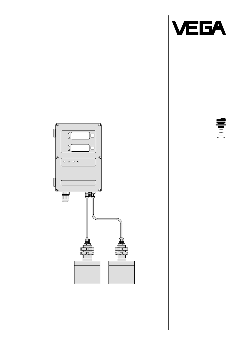
VEGASON

VEGASON 71 - 2 … 75 - 2

TIB • Technical Information • Operating Instructions

Pulse-Echo measuring system

Two channel operation 2-wire level measurement or

differential measurement Operating range up to

-5 m

- 10 m

- 20 m

- 30 m Compact unit with modules

for relay and current outputs Linearization Sensor optimization VEGASON 71 - 2 and 73 - 2

approved in hazardous areas of Ex - zone 1

5.00

Page 2

Contents

2 71 - 2 … 75 - 2

Introduction Contents of the instruction manual .....................................................4

Safety information ...............................................................................4

Special instructions for use in Ex-Zone 1 ...........................................4

Product description .............................................................................4

Technical Information Configuration of measuring system ....................................................5

Technical data ....................................................................................6

Dimensional drawing ..........................................................................8

Measuring range .................................................................................9

Installation examples - for liquid tanks ..........................................10

- for solids ..................................................11

Installation errors (tanks or silos) ......................................................11

Electrical connections .......................................................................12

Operating surface Indication and operating elements ....................................................13

Operating ..........................................................................................14

Start-up Flow diagram for start-up ..................................................................15

Mode listing 0, general parameter adjustments ................................16

Adjustment Level measurement ........................................................................20

Selection of the adjustment procedure .............................................20

Adjustment in m without level change ..............................................21

Adjustment in % with level change ...................................................21

Differential measurement ..............................................................22

Selection of the adjustment procedure .............................................22

Adjustment in m without level change ..............................................23

Linearization Adapting to the vessel geometry ......................................................24

Selection of the linearization curves 4 … 6 ......................................24

Mode listing 4 (5 and 6) ....................................................................25

Display demonstration ......................................................................25

Operation ..........................................................................................25

Determination of the index markers ..................................................26

Linearity protocol ..............................................................................27

Programming example .....................................................................28

Outputs Display function

Allocation of a multiplication factor ........................................29

Measuring units and pattern ..................................................29

Decimal point ........................................................................29

Module for relay outputs 1 … 4

Two-point level switch ...........................................................31

Pump function .......................................................................33

Tendency determination ........................................................35

Module for current output 1 and 2

Coordination and course of characteristics ...........................37

Page 3

Contents

71 - 2 … 75 - 2 3

Supplementary programming

Failure processing ............................................................................38

Simulation .........................................................................................39

Basic adjustment ..............................................................................40

Keyword ............................................................................................40

Sensor optimization Selection of sensor optimization .......................................................41

Mode listing 1 (2) sensor optimization ..............................................41

Information for sensor optimization ..................................................43

Limitation of the operating range

Start of operating range / end of operating range .............................44

Adapting

to the

product type ..........................................................................45

to the vessel geometry (liquid) ..........................................................45

to solids ............................................................................................46

Reduction of echo amplification

Multiple false echo reduction ............................................................47

Storage

of a false echo profile

False echo learn ....................................................................48

Profile interpolation ...............................................................49

Adapting

to filling and emptying speed

Rate of product level change ................................................50

Limitation

of the echo amplification

Max. gain ...............................................................................51

Supplementary optimization

Measuring window ............................................................................52

Fail safe ............................................................................................52

Real distance ....................................................................................53

Basic adjustment ..............................................................................53

Supplement

Protocol of sensor optimization ........................................................54

Error codes .......................................................................................55

Page 4

Product description

Introduction

4 71 - 2 … 75 - 2

Contents of the instruction manual

The Technical Information / Operating Instruc- tions is just called TIB. It contains all necessary information for correct:

- installation

- connection

- start-up

- linearization

- optimization the Pulse-Echo-measuring system VEGASON 71 - 2 … 75 - 2.

This TIB is supplied as part of the order. Knowledge of the contents is important for correct operation of the indicating instrument.

This TIB accompanies the product and is addressed to technical qualified staff which are trained or have knowledge of the use of level measurement and control equipment.

Safety information

The described module must only be inserted and operated as described in this TIB. Please note that other action can cause damage for which VEGA does not take liability.

VDE-regulations and the security measures valid for the respective applications should be observed.

Special instructions for the use in Ex-Zone 1

The transducers SW 71 … SW 73 (SW 71 applied) are also available in the Ex-flame proofing encapsulation "m". With the type designation SW 72 R and SW 73 R they have the flame proofing EEx m II T6 and can be used in Ex-Zone 1.

For these applications the regulations of the conformity certificate PTB-no. Ex–92.C.2113 as well as the special regulations acc. to VDE have to be observed. The above mentioned conformity certificate accompanies the instrument.

The Pulse-Echo-measuring system VEGASON 71 – 2 … 75 – 2 enables

- two channel level measurement or

- one differential measurement. The running periods of reflected sound impulse are

evaluated. The running period is a measure of the distance

between sensor (transducer) and product. The central electronics determines these distances

for each channel and converts them into the respective level.

Measurements are indicated on two integral LCdisplays and are either available as current or relay outputs.

A measuring system consists of

- one central electronics and

- two sensors (transducer). Each sensor has its own temperature sensor for

compensation of the temperature influence on the running period. The measuring data and temperature information are conducted via coax connection cable.

The measuring system is provided with factory-set parameters so that immediate use is possible for most applications.

The adjustment procedures and sensor optimizations etc. can be programmed directly via a keyboard on the central electronics.

Page 5

Technical Information

71 - 2 … 75 - 2 5

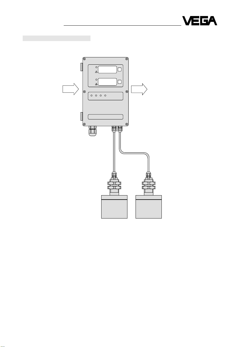
Configuration of a measuring system

Inputs Central electronics Outputs

Measuring data of transducer 1 channel 1

Measuring data of transducer 2 channel 2

Multi function indicator Module for relay output 1 and 2

Module for relay output 3 and 4 Module for current output 1 and 2

0 … 20 mA

Fail safe relay and fail safe-LEDs

1 2 3

VEGASON

Central electronics consists of:

- plastic housing with cover and integral

- operating elements (5 buttons)

- diodes (LED-indication)

- two multi function indications (LC-displays)

- power supply

- memory (EEPROM, no buffer battery required)

- outputs as modules (see above)

- terminals for power supply, inputs and outputs

Further instruments (option):

- indicating instrument VEGADIS 171 A (connection to 0 … 20 mA)

- overvoltage arrester

Transducer

Page 6

Technical data

Power supply operating voltage

standard U

nenn

= 24 V AC (16 … 42 V), 50 / 60 Hz = 24 V DC (16 … 60 V)

option U

nenn

= 230 V AC (90 … 250 V), 50 / 60 Hz

power consumption at U

nenn

and at max. load 12 VA / 5 W

fuse

for version 16 … 42 V AC or 16 … 60 V DC = 2 A

for version 90 … 250 V AC = 500 mA Type VEGASON 71 - 2 72 - 2 73 - 2 74 - 2 75 - 2 Minimum distance at liquids or 0,3 m 0,5 m –– –– ––

solids particle size ≥ 5 mm –– –– 0,8 m 0,8 m 1,0 m

particle size ≤ 5 mm –– –– 1,0 m 1,1 m 1,2 m

Maximum distance product and process dependent 5 m 5 m 10 m 20 m 30 m Input data min. measuring distance 10 cm 10 cm 10 cm 10 cm 10 cm

display in mm cm cm cm cm scanning 3 mm 3 mm 3 mm 3 mm 3 mm measuring frequency 50 kHz 40 kHz 33 kHz 22 kHz 16 kHz measuring rate 0,4 sec. 0,4 sec. 0,4 sec. 0,5 sec. 0,7 sec. angle of reflection at –3 dB) 7° 9° 12° 12° 12° linearity error acc. to empty / full adjustment < 0,1 % of measuring range temperature error of electronics 0,1 % / 10 k of measuring range

Sensor data number of transducer 2

transducer housing PVDF impedance adapter PE mounting tube type 71 … 73 PVDF, thread 1" BSP

type 74 and 75 RCH 1000, thread 1" BSP temperature sensor integrated in transducer permissible excess pressure in the vessel

- transducer 71 … 75 max. 1 bar

- transducer 71 R … 73 R max. 1 bar connection cable coax line type RG 58 line length standard 5 m

maximum 300 m cable diameter approx. 5 mm

Indication LC-display 2, 4-digits each Relay output max. 2 modules 2 relay 1 spdt per relay each

contact material AgCdO and Au plated min. turn-on voltage 10 mV

switching current 10 µA

max. turn-on voltage 250 V AC, 60 V DC

switching current 2 A AC, 1 A (DC)

max. breaking capacity 125 VA, 60 W

Technical Information

6 71 - 2 … 75 - 2

Page 7

Current outputs module - with 2 outputs

- range 0/4 … 20 mA

- resolution 0,05 % of range

- load max. 500 Ohm

- load dependent failure at 0 … 500 Ohm, < 0,2 % related to the range

or module - as above however with 2 floating outputs each

Fail safe function 1 relay for both channels 1 spdt

contact data as described under relay outputs 2 fail safe-LEDs separately per channel

Ambient ambient temperature on conditions - transducer 71 … 75 –20°C … +80°C / -4 … 176°F

- transducer 71 R … 73 R –20°C … +55°C / -4 … 131°F

- central electronics –20°C … +60°C / -4 … 140°F storage and transport temperature –20°C … +80°C / -4 … 176°F

Environmental protection protection - transducer 71 … 75 IP 68

- transducer 71 R … 73 R IP 68

- housing of central electronics IP 65 protection class II

Electrical terminals for max. 1 x 1,5 mm

connection cable entry 2 x Pg 7

1 x Pg 13,5, max. 5 x Pg 13,5

Material transducer PVDF

housing of central electronics Polycarbonate

Weight VEGASON 71 … 73 74 and 75

1 transducer (without cable) approx. 0,8 kg approx. 1,5 kg central electronics approx. 1,9 kg approx. 1,9 kg

Dimensions see dimensional drawing on following page

Technical Information

71 - 2 … 75 - 2 7

Technical data

(continuation)

Page 8

Technical Information

8 71 - 2 … 75 - 2

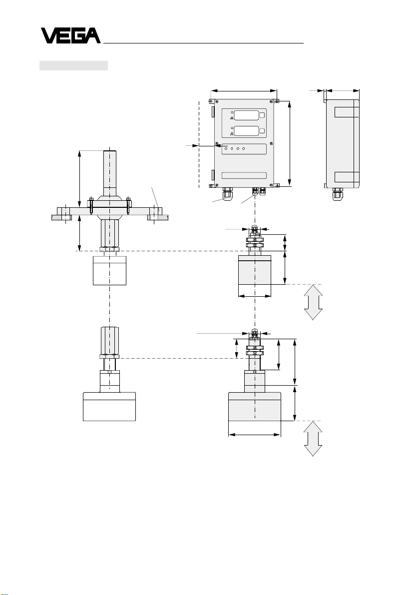
Dimensional drawing

(dimensions in mm)

411 2 3

VEGASON

*174

* Mounting dimensions

*229

Min. distance for

further instruments

ø95

appr. 100

Flange DN 150 PN 16

appr. 155

133

ø145

Sensor SW 72 / 73

Pg 13,5

Pg 7

Central electronics

G 1 A

Thread 1" BSP

0,5…0,8 m

0,8…1,2 m

Sensor SW 74 / 75

Flanged gimbal

Min. distance

Sensor SW 71 … 73 71 R … 73 R

Page 9

Technical Information

71 - 2 … 75 - 2 9

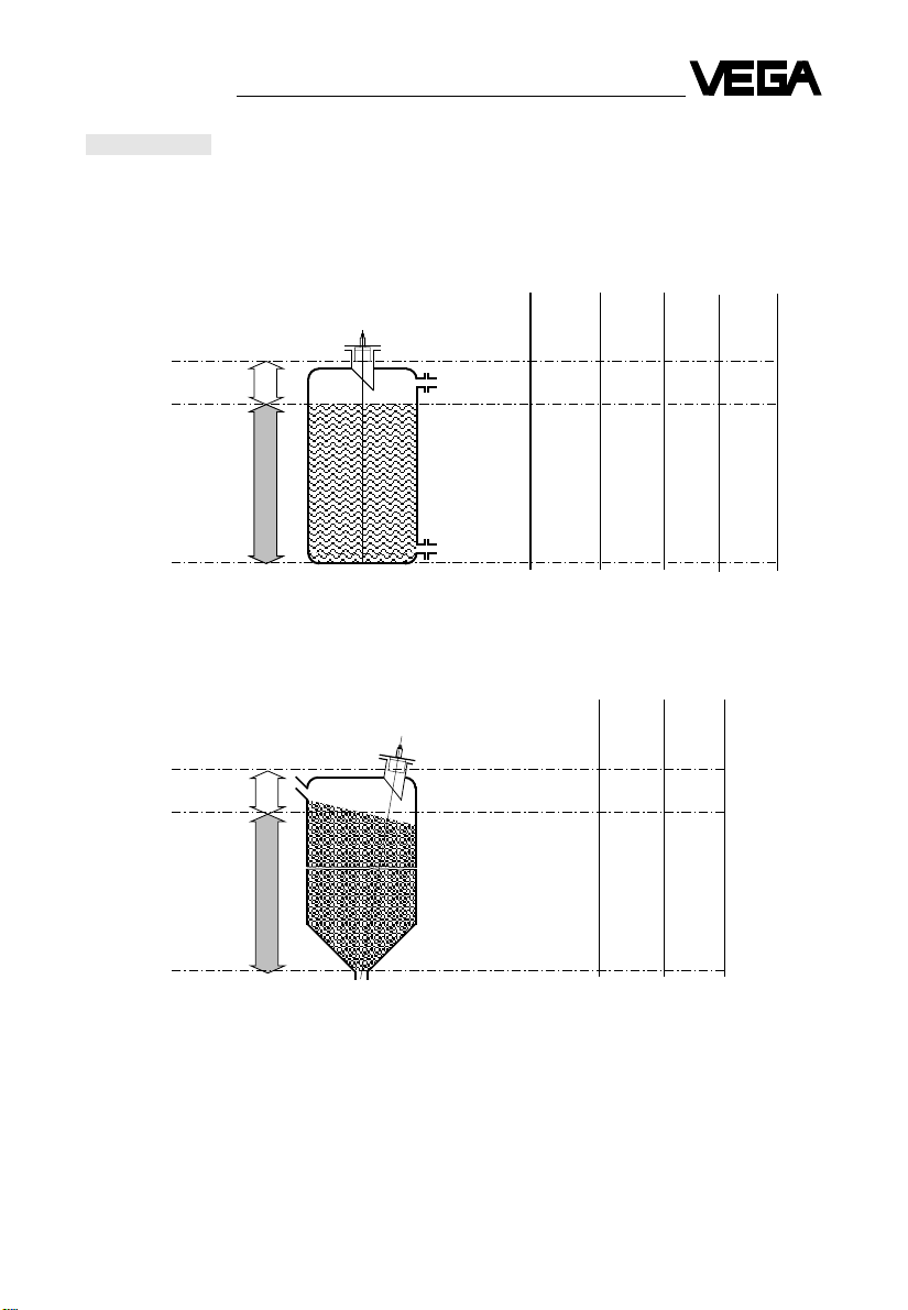
Measuring range

The measuring ranges described below are max. values and can change dependent on process conditions.

The location of the sensors should be carefully selected and it should be noted that no struts, edges or material inflow impede the measurement (see installation recommendations page 10 and 11).

for liquids

VEGASON 71 - 2 72 - 2 73 - 2 74 - 2 75 - 2

Reference pane

Min. distance 0,3 m 0,5 m 0,8 m 0,8 m 1,0 m

Measuring range

5 m 5 m 10 m 20 m 30 m

for solids

VEGASON 73 - 2 74 - 2 75 - 2

Reference pane

Min. distance particle size≥ 5 mm 0,8 m 0,8 m 1,0 m

particle size≤ 5 mm 1,0 m 1,1 m 1,2 m

Measuring range

10 m 20 m 30 m

Page 10

Technical Information

10 71 - 2 … 75 - 2

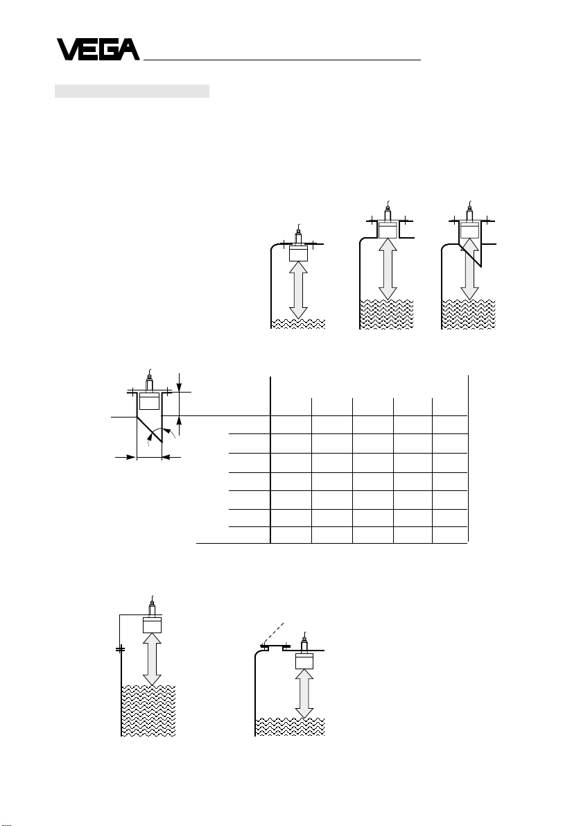
Installation example for liquid tanks

- Select sensor type and installation in relation to max. level to be measured.

- Protect the inner side of the socket piece for corrosion or use non-corrosive material.

- In case of round tank ceilings, the sensor should be installed on a socket piece not located in the centre or on an opening (on half radius).

In closed vessels:

Tube or direct mounting. If socket piece length > 100 mm or for VEGASON 72 / 73 or > 150 mm for VEGASON 74 / 75 are required (max. level). Note the dimensions in the following table.

in open vessels: Mounting via

Mounting by means access hatch: of bracketry Simple direct mounting

Max. socket piece length L at:

(dimensions in mm)

VEGASON 71 - 2 72 - 2 73 - 2 74 - 2 75 - 2

at socket 100 300 400 400 ––– ––– piece ø

150 300 500 400 300 300 200 ––– ––– 500 400 400 250 ––– ––– 600 500 500 300 ––– ––– ––– 600 600 350 ––– ––– ––– 700 700

Min. distance 300 500 800 800 1000

45°

Socket piece length

Page 11

Technical Information

71 - 2 … 75 - 2 11

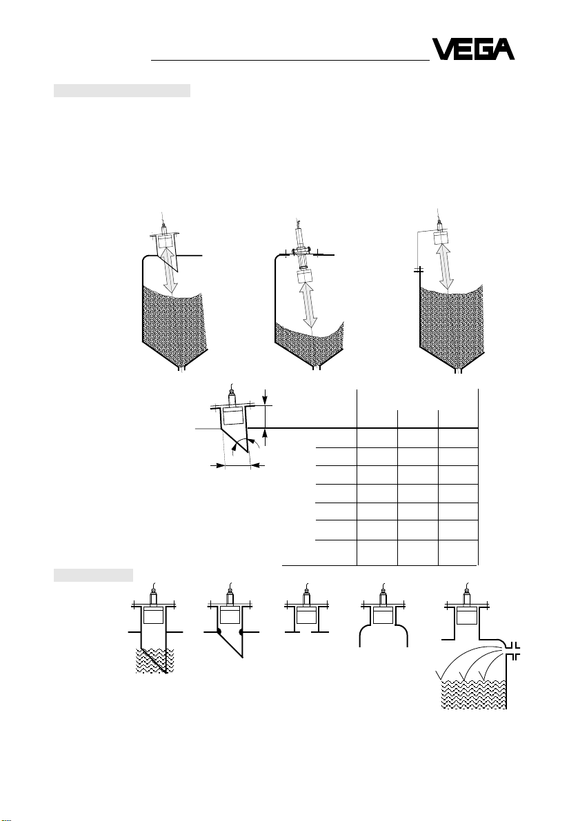
Installation examples for solids

- Select sensor type and installation in relation to max. level to be measured.

- Protect the inner side of the socket piece from corrosion or use non-corrosive material.

- Always direct the sensor (sound pulse) to the centre of the silo.

- Install sensor as far as possible from the filling entry.

- When using round ceilings, mount the sensor half way between silo middle and edge.

Installation with cylindrical socket piece

Installation with flanged gimbal

Installation in open silos via bracketry

socket piece length L at:

(dimensions in mm)

VEGASON 73 - 2 74 - 2 75 - 2

at socket 100 400 ––– ––– piece ø

150 400 300 300 200 500 400 400 250 600 500 500 300 ––– 600 600 350 ––– 700 700

Min. distance 800 … 800 … 1000 …

1000 1100 1200

Installation errors

(at tanks or silos)

45°

The socket piece should not be covered by the product.

The socket piece should not have weldment joints.

Access too small. Socket pieces in

the centre of round tank ceilings are not recommended for the sensor installation.

The beam should not cross the material inflow.

Page 12

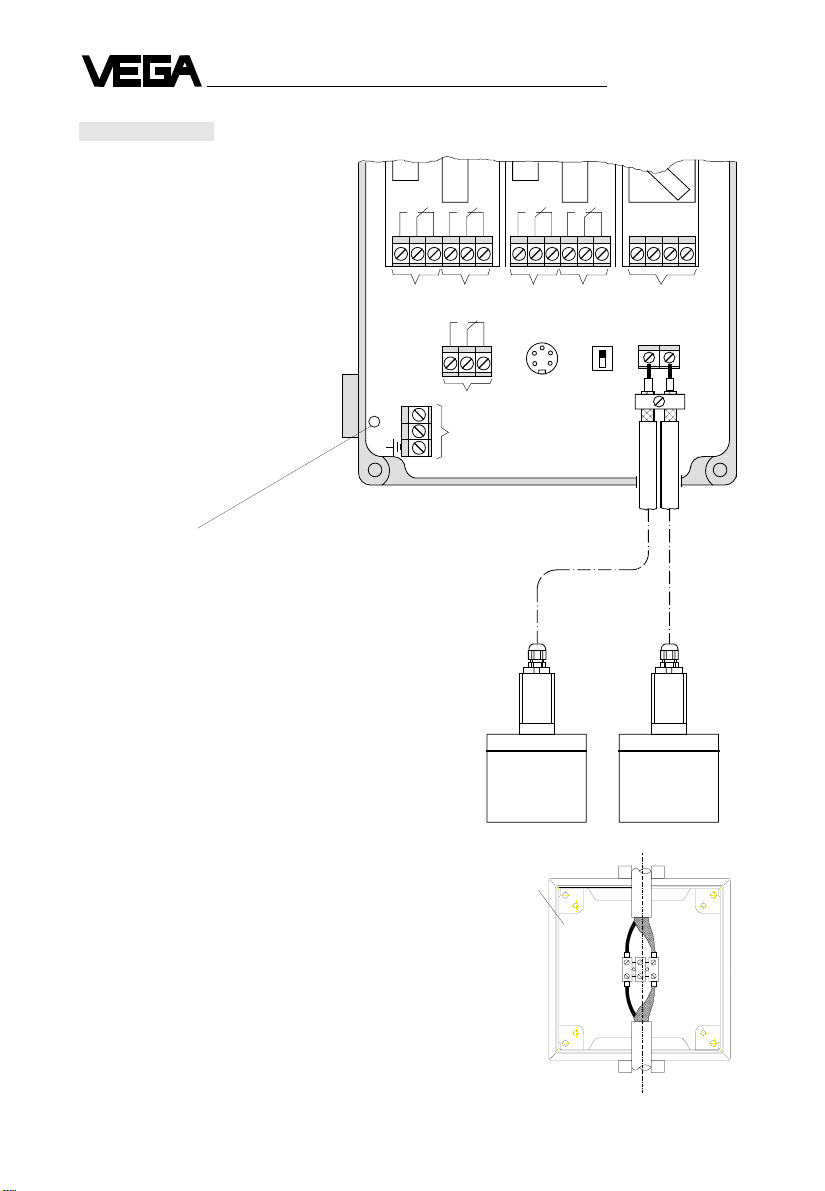
2 1

91011

13 14

21 22

15 16

+ - + -

Fail safe relay output

Supply voltage

Service socket

1 2

Service switch

1…………2 …………… 3………...4

Relay output

1………2

Current output

respective max. line length = 300 m

Sensor 1 Sensor 2

Channel 1

Channel 2

Technical Information

12 71 - 2 … 75 - 2

Electrical connection

Note:

During operation the transducer is pulsed with high voltages. It is therefore recommended that first all electrical connections are provided and then the power supply for the instrument switched on.

Attention!

Fuse Type TR5 Manufacturer e.g. Messrs. Wickmann Current values see technical data page 6

The connection line to the respective sensors can be extended afterwards as shown.

If must be observed that the max. line length of 300 m is not exceeded.

Standard waterproof dividing box

Page 13

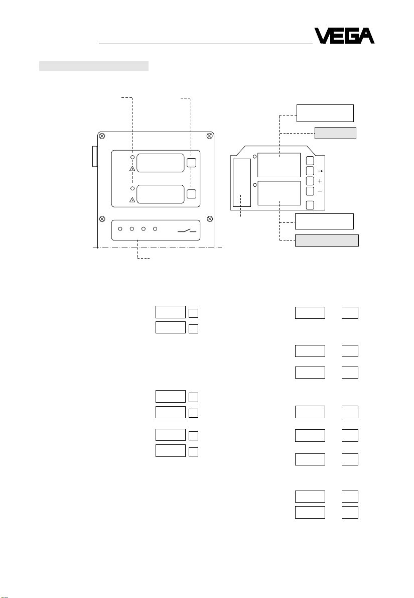
Operating surface

71 - 2 … 75 - 2 13

Indication and operating elements

Outer view Inner view

Indication of measured values

5.00 m

e.g. level 1 … 9 m

5.00 m

Demonstration form after programming of - multiplier

- allocation of decimal point

- decimal point e.g.

50.0 %

level 0 … 100 %

5.00 %

2000 hl

level 0 … 4000 hl

2000 hl

Mode range

general reset 0 - 00 … 99

sensor optimization 1 1 - 01 … 27

sensor optimization 2 2 - 01 … 27

linearization curve 4 4.H.01 … 32

linearization curve 5 5.H.01 … 32

linearization curve 6 6.H.01 … 32

fault signals channel 1 E2.01 … .04

channel 2 E2.01 … .04

1 2 3

MOD

STO

MODEFIELD

Indication of measured values 1

PARAMETER FIELD

Indication of measured values 2

8888

8888 8888

8888

LED-indication of relay outputs 1…4

Operating scheme

LED-indication fault signal channel 1 and 2

Units indicator visible in slot behind window

Selection of mode

Cursor position Figures raise Figures lower

Storage

Page 14

Operating surface

14 71 - 2 … 75 - 2

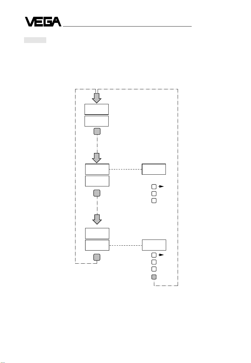
The VEGASON 71 - 2 … 75 - 2 has 3 modes which can be accessed (scrolling) via the MOD-button:

Mode: 1. indication of measured values

2. mode range

3. parameter input

If no push button is used for a 60 minutes period, the VEGASON 71 - 2 … 75 - 2 times out and reverts to the input value display.

Operating

In mode 99 the main stage 0 can be left and stage 1 and 4 … 6 can be selected. The reset to main stage 0 is done in the respective mode 99.

During a parameter adjustment the last mode number used is activated again after each STOcommand and entry to the mode range.

Indication of measured values: level in m level in % and acc. to the demonstration form e.g. quantity in hl.

For selection of the mode numbers see MODEFIELD. The parameters of the selected mode numbers can be checked or modified in mode 3.

Programming of parameters see PARAMETER FIELD. The parameters of the selected mode can be modified and stored with STO-button. With STO reset to mode 1.

MOD

STO

Cursor position Figures raise Figures lower

5.00

0 00000

16.93

0 99

0 - 00

– – – –

1. Indication of measured values

2. Mode range

3. Parameter adjustment

Page 15

Start-up

71 - 2 … 75 - 2 15

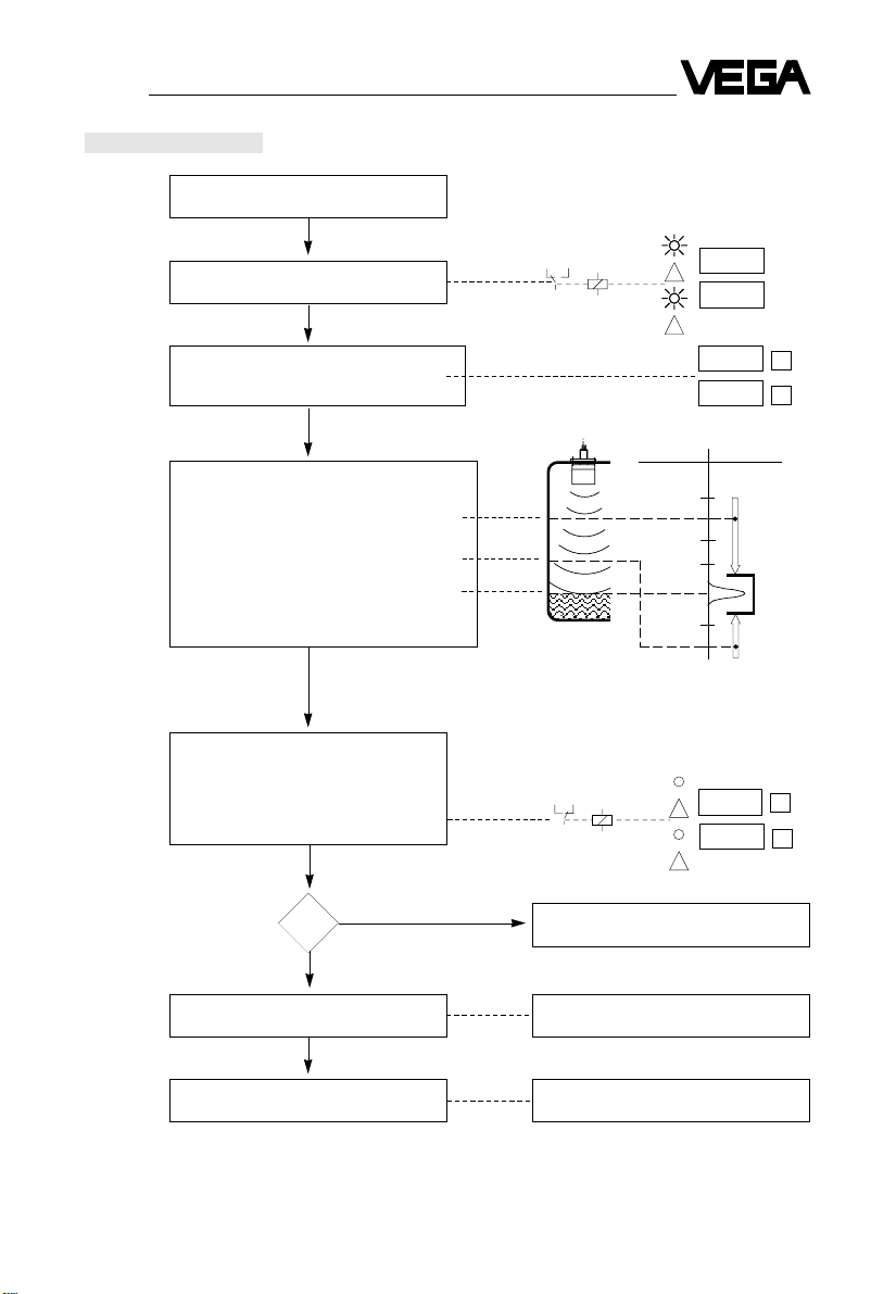
Flow diagram for start-up

Connect sensors with central electronics and supply with operating voltage.

The software version is indicated and the fault signal reacts.

The measuring system is now ready and starts for each separate channel with the commissioning preliminary indication: 0.00 m.

Commissioning, i.e.:

1. Echo limitation from top to bottom.

2. Echo limitation from bottom to top.

3. Formation of a measuring window within which an evaluation of the echo is carried out.

After approx. 1 … 3 minutes the measuring system is ready. The fault signal extinguishes. The sensors 1 and 2 adapted to the vessel feature and operate with the parameters of the VEGA-adjustments.

Level measurement 1

Level measurement 2

Sensor 2 determines in vessel 2 the actual distance of 9,50 m

Sensor 1 determines in vessel 1 the actual distance of 9,20 m

Optimizations are necessary for sensor 1 and / or sensor 2

YES

5 6

14.94

5 6

9.20

9.50

0.00

Page 16

Start-up

16 71 - 2 … 75 - 2

Mode listing 0

Function Mode-no. Mode description Parameter Page

( = factory preset)

0 - 00 Software version ........................................ e.g. 16.93

0 - 01

… 09 not used ..................................................... – – – –

Adjustment 0 - 10 Selection of adjustment procedure channel 1

- in m without level change ....................... 1

- per cent correction .................................. 2

- in % with level change ........................... 3

0 - 11

Empty adjustment

- distance in m........................................... sensor specific p. 20

- level in % ................................................ 0.0 … 80.0

0 - 12

Full adjustment

- distance in m........................................... sensor specific

- level in % ................................................ 100.0 … 20.0

Display Multiplier

function 0 - 13 - related to 0 % ......................................... 0000 … 9999

0 - 14 - related to 100 % ..................................... 0000 … 1000 … 9999

0 - 15 Measuring unit

- level percentage in m ............................. 1 p. 29

- level percentage in % ............................. 2

- volume percentage (scaled) ................... 3

0 - 16 Decimal point............................................ 0.000 … 000.0 … 0000

0 - 17 Integration time ........................................ 0 … 900

Lineari- 0 - 18 Linearization curves

zation - linear ...................................................... 1

- cylindrical tank ........................................ 2

- not used ................................................. 3 p. 24

- individually programmable curve 4 ......... 4

- individually programmable curve 5 ......... 5

- individually programmable curve 6 ......... 6

0 - 19 not used ..................................................... – – – –

Adjustment 0 - 20 Selection of adjustment procedure

channel 2 - in m without level change ....................... 1

- per cent correction ................................. 2

- in % with level change ........................... 3

0 - 21 Empty adjustment

- distance in m........................................... sensor specific p. 20

- level in % ................................................ 0.0 … 80.0

0 - 22 Full adjustment

- distance in m........................................... sensor specific

- level in % ................................................ 100.0 … 20.0

general parameters

Page 17

Start-up

71 - 2 … 75 - 2 17

Mode listing 0 general parameters

Display Multiplier

function 0 - 23 - related for 0 % ........................................ 0000 … 9999

0 - 24

- related for 100 % .................................... 0000 … 1000 … 9999

0 - 25

Measuring unit

- level percentage in m ............................. 1 p. 29

- level percentage in % .............................

- volume percentage (scaled) ................... 3

0 - 26 Decimal point ........................................... 0.000 … 000.0 … 0000

0 - 27 Integration time ........................................ 0 … 900

Lineari- 0 - 28 Linearization curves

zation - linear ...................................................... 1

- cylindrical tank ........................................ 2

- not used ................................................. 3 p. 24

- individually programmable curve 4 .........

- individually programmable curve 5 ......... 5

- individually programmable curve 6 ......... 6

0 - 29 not used ..................................................... – – – –

Adjustment 0 - 30 Selection of adjustment procedure

differential - in m without level change ....................... 1

measure- - percent correction .................................. 2

ment 0 - 31 Adjustment min. difference

- in m ......................................................... sensor specific p. 22

- percent correction .................................. 0.0 … 80.0

0 - 32 Adjustment max. difference

- in m ......................................................... sensor specific

- percent correction .................................. 100.0 … 20.0

Display Multiplier

function 0 - 33 - related to 0 % ......................................... 0000 … 9999

0 - 34 - related to 100 % ..................................... 0000 … 1000 … 9999

0 - 35 Measuring unit

- level percentage in m ............................. 1 p. 29

- level percentage in % ............................. 2

- volume percentage (scaled) ................... 3

0 - 36 Decimal point ........................................... 0.000 … 000.0 … 0000

0 - 37 … 39 not used ..................................................... ––––

Display 0 - 40 Display coordination

1 1 0 = inactive p. 22

Display 2 1 = level indication

(channel specific)

Display 1

2 = differential indication

0 - 41 u. 42 not used ..................................................... – – – –

Function Mode-no. Mode description Parameter Page

( = factory preset)

(continuation)

Page 18

Start-up

18 71 - 2 … 75 - 2

Mode listing 0 general parameters

Function Mode-no. Mode description Parameter Page

( = factory preset)

(continuation)

Relay 0 - 43 Coordination

output 1 - channel 1 ................................................ in m = 1 in % = 2

- channel 2 ................................................ 34

- difference ............................................... 56p. 31

0 - 44 Mode

- two-point level switch ............................. 1

- pump function switch .............................. 2

- tendency determination raising .............. 3

- tendency determination lowering ........... 4

0 - 45 Switching 1 (on) ............................. sensor specific

0 - 46 command 2 (off) ............................. sensor specific

0 - 47 Indication of running period ....................... indication in 10 h-units

Relay 0 - 48 Coordination

output 2 - channel 1 ................................................ in m = 1 in % = 2

- channel 2 ................................................ 34

- difference ............................................... 56p. 31

0 - 49 Mode

- two-point level switch ............................. 1

- pump function switch .............................. 2

- tendency determination raising .............. 3

- tendency determination lowering ........... 4

0 - 50 Switching 1 (on) ............................. sensor specific

0 - 51 command 2 (off) ............................. sensor specific

0 - 52 Indication of running period........................ indication in 10 h-units

Relay 0 - 53 Coordination

output 3 - channel 1 ................................................ in m = 1 in % = 2

- channel 2 ................................................ 34

- difference ............................................... 56p. 31

0 - 54 Mode

- two-point level switch.............................. 1

- pump function switch .............................. 2

- tendency determination raising .............. 3

- tendency determination lowering ........... 4

0 - 55 Switching 1 (on) ............................. sensor specific

0 - 56 command 2 (off) ............................. sensor specific

0 - 57 Indication of running period ....................... indication in 10 h-units

Relay 0 - 58 Coordination

output 4 - channel 1 ................................................ in m = 1 in % = 2

- channel 2 ................................................ 34

- difference ............................................... 56p. 31

0 - 59 Mode

- two-point level switch ............................. 1

- pump function switch .............................. 2

- tendency determination raising .............. 3

- tendency determination lowering ........... 4

0 - 60 Switching 1 (on) ............................. sensor specific

0 - 61 command 2 (off) ............................. sensor specific

0 - 62 Indication of running period ....................... indication in 10 h-units

0 - 63 Interval time for pump function .................. 0000 … 9999 p. 34

Page 19

Start-up

71 - 2 … 75 - 2 19

Mode listing 0 general parameters

Function Mode-no. Mode description Parameter Page

( = factory preset)

(continuation)

Current 0 - 64 Coordination - channel 1 ..................... 1

output 1 - channel 2 ..................... 2

- difference ..................... 3 p. 37

0 - 65 Charac- - end ............................... 20.00 … 00.00

0 - 66

teristics - start .............................. 00.00 … 04.00 … 20.00

0 - 67

not used ..................................................... – – – –

Current 0 - 68 Coordination - channel 1 ..................... 1

output 2 - channel 2 ..................... 2

- difference...................... 3 p. 37

0 - 69 Charac- - end................................ 20.00 … 00.00

0 - 70

teristics - start .............................. 00.00 … 04.00 … 20.00

0 - 71 … 92 not used ..................................................... – – – –

0 - 93 Fault signal processing

store actual current

1 1 1 switching relay p. 38

difference unchanged = 1 channel 2 current 0 mA channel 1 switching relay

de-energizes = 2 current goes to 0 % switching relay de-energizes = 3 current goes to 100 % switching relay de-energizes = 4

0 - 94 Simulation - channel 1 0 - 95 - channel 2 sensor specific in m p. 39 0 - 96 - difference

0 - 97 Basic - switched off .................. 0 p. 40

adjustment - switched on .................. 1

0 - 98 Keyword - switched off ................... 0 p. 40

- switched on .................. 1

0 - 99 Change - general parameter ................ 0

- sensor optimization 1 ........... 1

- sensor optimization 2 ........... 2 p. 41

- linearization curve 4 ............. 4

- linearization curve 5 ............. 5

- linearization curve 6 ............. 6

Page 20

Adjustment at level measurement

20 71 - 2 … 75 - 2

Level measurement

Two separate level measurements can be obtained with the VEGASON 71 - 2 … 75 - 2 (measuring system).

The adjustment is carried out for

- level measurement 1 = measuring channel 1 in mode range no. 10 … 12

- level measurement 2 = measuring channel 2 in mode range no. 20 … 22

The adjustment procedures are carried out separately for each sensor.

The display coordination is programmable and supplied as factory preset in mode 40 as follows:

0 – 4 0

1 1

level 2 (display 2) level 1 (display 1)

Selection of adjustment procedure

The type of empty adjustment (mode 11) and full adjustment (mode 12) is determined with the parameter adjustment of this mode.

The type of adjustment depends on the local conditions.

Mode description

Mode 10 = 1 means adjustment in m without product level change, i.e.

- with this adjustment procedure the distances in m determined from the vessel drawings are programmed relating to the levels 0 % and 100 %

- level is not important

Mode 10 = 3 means adjustment in % without product level change, i.e.

- with this adjustment procedure the levels are programmed in % and the respective measured distance (sensor … level) is calculated automatically

- product level change is needed.

Programming example

Change of mode 10 = 3 of mode 10 = 1 .................. • select mode 0 - 10 in MODEFIELD

• program figure1 in PARAMETER FIELD

• then store with STO-button

Same procedure for channel 2, however mode 0 - 20.

Demonstration

Mode 10 = 1 Mode 10 = 3

Min. distance ^ 100 %

partly filling = e.g. 75 %

partly emptying

= e.g. 25 % Max. distance ^0 %

MODE 0 - 10

Page 21

Adjustment at level measurement

71 - 2 … 75 - 2 21

Empty / full adjustment in m without product level change

Programming pre-requirement

Mode 10 = 1 Mode 40 = 11

With this adjustment procedure two distances (sensor … product surface) are defined in m relating to the levels of 0 % and 100 %.

MODE 0 - 11 and 0 - 12

Programming example with VEGASON 73 - 2 (individual programming sequence of the empty /

full adjustment)

• select mode 0 - 12 in MODEFIELD

• program 01.00 m in PARAMETER FIELD

• then store with STO-button

• select mode 0 - 11 in MODEFIELD

• program 09.00 m in PARAMETER FIELD

• then store with STO-button

Empty / full adjustment in % with product level change

Programming pre-requirement

Mode 10 = 3 Mode 40 = 11

MODE 0 - 11 and 0 - 12

Programming example with VEGASON 73 - 2 (individual programming sequence of the empty /

full adjustment)

• select mode 0 - 12 in MODEFIELD

• program 075.0 % in PARAMETER FIELD

• then store with STO-button

• select mode 0 - 11 in MODEFIELD

• program 025.0 % in PARAMETER FIELD

• then store with STO-button

With this adjustment procedure two levels are defined in % relating to two different, actually measured distances (sensor … product surface).

The difference should be as large as possible. The central electronics determines the adjusted range (e.g. 25 … 75 %) from the total range (0 … 100 %).

Same procedure for channel 2, however mode 0 - 21 and 0 - 22.

distance

100

m0%

1 m distance

^ 100 %

9 m distance

^0 %

19100

measured

distance

^ 75 %

measured

distance

^ 25 %

m0%

level

distance level

Page 22

Adjustment at differential measurement

22 71 - 2 … 75 - 2

Differential measurement

A differential measurement can be obtained with the measuring system VEGASON 71 - 2 … 75 - 2.

The difference is formed out of the values of channel 2 minus channel 1. If possible, mount the sensors at the same height.

The adjustment is made for both measuring channels together in mode range no. 30 … 32.

It is possible to adjust channels 1 and 2 separately as described under level measurement.

The display coordination is defined as follows in mode 0 - 40:

0 - 4 0

1 1

0 = display 2 switched off 1 = display 2 indicates level

of channel 2

2 = display 2 indicates difference 0 = display 1 switched off

1 = display 1 indicates level

of channel 1

2 = display 1 indicates difference

The pre-adjustment 1 for mode 0 - 30 should not be changed.

Mode description

Mode 0 - 30 = 1 mean adjustment in m without product level change, i.e.

- with this adjustment procedure various differences (levels, gauges etc.) are programmed relating to the values 0 % and 100 %

- already available levels or water gauges are unimportant

Selection of adjustment procedure MODE 0 - 30

MODE 0 - 40

Programming example

for - differential level on display 1

- level 2 (downstream water) on display 2 ....... • select mode 0 - 40 in MODEFIELD

• program figure 21 in PARAMETER FIELD

• then store with STO-button

Page 23

Adjustment at differential measurement

71 - 2 … 75 - 2 23

Differential adjustment in m without differential measurement

Programming as pre-requirement

Mode 30 = 1 Mode 40 = 21 or 12, display coordination

With this adjustment procedure two differences in m are defined, relating to the values of 0 % and 100 %.

MODE 0 - 31 and 0 - 32

Programming example 1

with VEGASON 71 - 2 mounted at the same height for weir control.

(Individual programming sequence of the min. / max. difference)

• select mode 0 - 31 in MODEFIELD

• program 00.00 m in PARAMETER FIELD

• then store with STO-button

• select mode 0 - 32 in MODEFIELD

• program 01.00 m in PARAMETER FIELD

• then store with STO-button The level difference can occur within the whole

range (in the example e.g. 0 … 5 m) and can be detected.

Programming example 2 as above, however sensors mounted at different height

program 0 m + 0,5 m = 0,5 m respective 0 % in mode 31 = 00.50 m

program 1 m + 0,5 m = 1,5 m respective 100 % in mode 32 = 01.50 m

Further adjustment of channel 1 and 2 Upstream adjustment Full adjustment mode 0 - 12 = 01.00 m program distance

(channel 1) Empty adjustment mode 0 - 11 = 05.00 m program distance Downstream adjustment Full adjustment mode 0 - 22

(channel 2) example 1 = 01.00 m or

example 2 = 01.50 m program distance

Empty adjustment mode 0 - 21

example 1 = 05.00 m or example 2 = 05.50 m program distance

m 0

distance level

channel 1

upstream liquid

Max-difference 1 m

^ 100 %

Min-difference 0 m

^0 %

downstream liquid

∆ = 1m

100

channel 2

+ 0,5

m 0

100

channel 1

distance level

upstream liquid

min-difference

max-difference

downstream liquid

channel 2

The value of the sensor in the plus range of channel 2 must be added to the min. and max. distance

Page 24

Linearization

24 71 - 2 … 75 - 2

Linearization

Adapting to vessel geometry (channel 1)

The most usual vessel geometries are adjusted as fixed curves in mode 0 - 18.

Mode 0 - 18 = 1 Fixed curve (linear) level percentage

for cylindrical tank output

Mode 0 - 18 = 2 Fixed curve for volume percentage

cylindrical tank output

It is also possible to program three customer specific curves by accessing linearization 4 … 6 and to activate them in mode 18.

Each linearization curve consists of max. 32 index markers, each index marker of a H/L-pair.

Mode 0 - 18 = 4 linearization curve 4 volume percentage

5 5 output 66

Output condition for the level in litres see page 26, related to channel 1

- adjustment related to 0 % and 100 %, is carried out

- Mode 0 - 15 = 3 (1 level percentage)

- Mode 0 - 18 = 1

- total volume of the vessel is known (for the following example 100 m

)

- part volume for gauging the capacitance in litres is known (for the following example = 5 m

)

Same procedure for channel 2.

MODE 0 - 18

Selection of linearization curve 4 … 6

Each linearization curve 4 … 6 can be accessed in mode 0 - 99 and the reset carried out.

MODE 0 - 99

Programming example Linearization 4 ............. • select mode 0 - 99 in MODEFIELD

• program figure 4 in PARAMETER FIELD

• then store with STO-button

• push MOD-button to select index markers Reset in mode 99 with figure 0 in PARAMETER

FIELD.

Selection of linearization curve 4 … 6

Reset to general parameter adjustment

0 - 99

0 - 01

4H.01

5H.01

6H.01

4 - 99

Page 25

Linearization

71 - 2 … 75 - 2 25

Display

number of the linearization curve 4 … 6 indication for level percentage = H

indication for volume percentage = L number of index marker 01 … 32

Display 1 4 . H . 0 1 MODEFIELD

Display 2 1 0 0 . 0 PARAMETER FIELD

Mode listing 4 Linearization curve 4 … 6

Function Mode-no. Mode description Parameter

( = factory preset)

Index 4.H.01 1. index - level percentage ........... 000.0 … 100.0

marker 4.L.01 marker - volume percentage ...... 000.0 … 100.0

•

4.H.32 32. index - level percentage ........... 000.0 … 100.0

4.L.32

marker - volume percentage ...... 000.0 … 100.0

4 - 33

… 98 not used ..................................................... – – – –

4 - 99 Change - general parameter ............. 0

- sensor optimization 1 .......... 1

- sensor optimization 2 .......... 2

- linearization curve 4 ............ 4

- linearization curve 5 ............ 5

- linearization curve 6 ............ 6

Linearization curve 4

Linearization curve 5 see above, however 5.H.01 … 5.H.32

5.L.01 … 5.L.32 5 - 99

Linearization curve 6 see above, however 6.H.01 … 6.H.32

6.L.01 … 6.L.32 6 - 99

Proceeding

4.H.011

4.HHHH.01 4.H.00001 4.H.011

scrolling with button

→

100.0

4.LLLL.01 4.H.99991 4.H.099

by scrolling with

button plus or minus

Page 26

Linearization

26 71 - 2 … 75 - 2

Determination of the index markers

Gauging the level in litres

- mode 40: coordinate display 1 to level 1

- mode 99: select linearization curve 4

- fill or empty step by step with part volume

- note the respectively measured values for H % (level percentage) of display 1 on the linearity protocol

- the respective value for L % (volume percentage) should be calculated as follows

100 % x part volume1 (…32)

L % = ––––––––––––––––––––––––

vessel volume

e.g. volume percentage for 1 part volume:

100 % x 5 m

L % = –––––––––––– = 5 % (acc. to example)

100 m

- note the calculated values for L % in the linearity protocol

- continue the procedure of "gauging the level in litres" with the same part volume until H 100 % and L 100 % as described above.

- Attention: The linearization curves must ALWAYS be finished with H 100 % and L 100 %. This finish can be programmed after any number of index markers.

Demonstration to the following programming example (see page 27)

Heights %

Volume %

etc.

level perc. 02

level perc. 01

100

10 20 30 40 50 60 70 80 90

100

100.0

12.0

4.H.01

4.L.01

4.L.32

5.0 100.0

4H.32

index marker

01 … 32

index marker 01 … 32

Page 27

Linearization

71 - 2 … 75 - 2 27

Linearity protocol

Linearization curve index level percentage volume perc.

marker no. H L 01 02 03 04 05 06 07 08 09 10 11 12 13 14 15 16 17 18 19 20 21 22 23 24 25 26 27 28 29 30 31 32

Date

Name

Linearization curve index level percentage volume perc.

marker no. H L 01 02 03 04 05 06 07 08 09 10 11 12 13 14 15 16 17 18 19 20 21 22 23 24 25 26 27 28 29 30 31 32

Date

Name

Page 28

Linearization

28 71 - 2 … 75 - 2

Programming example:

Index marker 01........................................................ • index marker 01 4.H.01

select level percentage MODEFIELD

Level percentage ...................................................... • acc. to linearity protocol program 12.0 % in

PARAMETER FIELD

• then store with STO-button

• index marker 01 4.L.01 select volume percentage MODEFIELD

Volume percentage................................................... • acc. to linearity protocol program 5 % in

PARAMETER FIELD

• then store with STO-button

Index marker 02 ....................................................... • index marker 02 4.H.02

select and program the data as described above etc.

After programming is finished .................................. i.e. transmission of all data noted in the linearity

protocol,

- reset factory settings

- mode 0 - 15 = 3 (volume percentage)

- activate linearization curve 4 in mode 0 - 18

(mode 0 - 18 = 4)

Same procedure for linearization curve 5 and 6.

Page 29

Measurement, Display function

71 - 2 … 75 - 2 29

Multiplier

for 0 % and 100 % (channel 1)

(channel 1)

MODE 0 - 13 and 0 - 14

Values of 0000 … 9999 can be coordinated to levels 0 % and 100 % after the adjustment procedure.

The central electronics calculates all intermediate values out of this data.

Measuring units and pattern MODE 0 - 15

Programming possibilities:

Mode combination

Demonstration / vessel geometry Measuring unit Measuring unit Linearization

0 - 15 0 - 18

Percentage level m / % / scaled m 1

1 scaled 3 (Mode 0 - 13, 0 - 14 and 0 - 16)

Percentage volume % / scaled % 2

2 scaled 3 and (Mode 0 - 13, 4 … 6 0 - 14 and 0 - 16)

Decimal point MODE 0 - 16

Summary

The display can be adjusted to a specific application by combinations of these modes and adaption of their parameters.

Mode 0 - 13 and 0 - 14

values of 0000 … 9999

2005 hl

Mode 0 - 16

position of decimal point

Mode 0 - 15

measuring unit (pattern)

The position of the decimal point can be determined in mode 16.

In mode 0 - 15 the signal conditioning instrument can be defined for the display either (proportional) volume or level. Measuring units can be selected and slotted into the window.

Pattern for: % m cm ft kg t gal hl m

Page 30

Measurement, Display function

30 71 - 2 … 75 - 2

Programming example

After multiplying

- the distance corresponds to 9 … 1 m

- the level corresponds to 10 … 4000 hl

(10 hl = min. quantity)

Example display 10 hl … 4000 hl

Multiplier for 0 % ...................................................... • select mode 0 - 13 in MODEFIELD

• program the value 001.0 in PARAMETER FIELD

• then store with STO-button The actual distance of 5.00 (m)

remains indicated on display 1.

Multiplier for 100 % .................................................. • select mode 0 - 14 in MODEFIELD

• program the value 400.0 in PARAMETER FIELD

• then store with STO-button The actual distance of 5.00 (m)

remains indicated on display 1.

Measuring unit and pattern ...................................... • select mode 0 - 15 in MODEFIELD

• program the figure 3 in PARAMETER FIELD

• then store with STO-button 50 % of the previously programmed

multiplication factor (

^ 199.5) plus

the min. quantity (

^ 1,0) is indicated

on the display, i.e.

Position of decimal point .......................................... • select mode 0 - 16 in MODEFIELD

• shift with button

→ the position of the decimal

point 1 x to the right

• then store with STO-button The desired range is displayed.

Insert pattern hl.

Follow the same procedure for channel 2, but use modes 0 - 23 … 0 - 26 or for differential measurement, modes 0 - 33 … 0 - 36.

100 %

Mode 14

Mode 13

4000 hl

2005

100

Mode 15+16

1 m

5 m

9 m

NiveauDistanz

5.00

2005

5.00

200.5

2005

Distance level

(linearized)

Page 31

Measurement, Relay output

71 - 2 … 75 - 2 31

Module for relay output 1 … 4

The pulse-echo measuring system can be equipped with max. two relay modules.

Each module has two relay outputs.

Two-point level switch

Mode coordination / meaning module relay coordi- mode switching command

output nation 1 and 2

1 1 0 - 43 0 - 44 = 1 0 - 45 and 0 - 46

2 0 - 48 0 - 49 = 1 0 - 50 and 0 - 51

2 3 0 - 53 0 - 54 = 1 0 - 55 and 0 - 56

4 0 - 58 0 - 59 = 1 0 - 60 and 0 - 61

Coordination

(Module 1, relay output 1)

MODE 0 - 43

For each relay output the coordination can be programmed separately and relates to:

- measurement (channel 1, 2 and difference)

- measuring unit

- level / volume percentage

vessel geometry / measuring result measuring unit coordination linearization

(channel definition) 0 - 43 0 - 18, 0 - 28

level percentage channel 1 m = 1

% = 2 0 - 18 = 1

channel 2 m = 3

% = 4 0 - 28 = 1

difference m = 5

%= 6

volume percentage channel 1 % = 2 0 - 18 = 2

or 4 … 6

channel 2 % = 4 0 - 28 = 2

or 4 … 6

difference % = 6

Mode

(Module 1, relay output 1)

MODE 0 - 44

Mode 0 - 44 = 1 two-point level switch switching command 2 via switching command 1 correspond to function A (overfill protection)

100

% m

distance acc.t o sensor type

mode combination

switching command 2, mode 0-46

switching command 1, mode 0-45

(off)

(on)

Page 32

Measurement, Relay output

32 71 - 2 … 75 - 2

Mode

(Module 1, relay output 1) continuation

Mode 0 - 44 = 1 two-point level switch switching command 1 via switching command 2 correspond to function B (protection against dry running of pumps)

Switching command 1 and 2

(Module 1, relay output 1)

MODE 0 - 45 and 0 - 46

Mode 0 - 43 defines the measurement units coordinated to the relay output.

Mode 0-44 determines the function of the relay output.

Mode 0-45 = switching command 1 corresponds

relay switched on (on)

Mode 0-46 = switching command 2 corresponds

relay switched off (off)

With the operating sequence of the switching commands, the A- or B-function i.e. overfill protection or protection against dry running of pumps is determined. See page 31 and 32.

The min. ∆ for the switching commands is 10 cm or 0,5 %.

Programming example for relay output 1 ............... - coordination to channel 1 with units in %

- mode 1

- two-point level switch in function A (see page 31)

Coordination (channel 1 in %) .................................. • select mode 0 - 43 in MODEFIELD

• program figure 2 in PARAMETER FIELD

• then store with STO-button

Mode (two-point level switch).................................... • select mode 0 - 44 in MODEFIELD

• program figure 1 in PARAMETER FIELD

• then store with STO-button

Switching command 1 (on) ...................................... • select mode 0 - 45 in MODEFIELD

• program 025.0 % in PARAMETER FIELD

• then store with STO-button

Switching command 2 (off) ....................................... • select mode 0 - 46 in MODEFIELD

• program 050.0 % in PARAMETER FIELD

• then store with STO-button

Same function and procedure for module 1, relay output 2 and module 2, relay output 3 and 4, however with respective modes, see page 31.

100

% m

distance acc. to sensor type

switching command 1, Mode 0-45

switching command 2, Mode 0-46

(off)

(on)

Page 33

Measurement, Relay output

71 - 2 … 75 - 2 33

Using the VEGASON-measuring system in pump stations allows several pumps to be used independent of the level. Due to the different switching commands there could be unequal pump running times (and wear).

With programming the mode "pump function" the switch on period of the respective relay outputs is monitored via the central electronics. An automatic change-over (priority determination) ensures equality of pump running periods. See the following example with three pumps.

Priority determination by:

- switching on the measuring system

- all relay outputs concerned in the pump function switched off, i.e. with all pumps

- with time interval, the time interval is active if within the time programmed in mode 63 all pumps are

not stopped. In this case first all relay outputs are switched off, the actual priority will be determined and the pumps will be switched on again in new sequence after 10 secs.

Factory preset of mode 0 - 63 with 9999 minutes ^ approx. 1 week to the max interval time.

Note:

Before changing this time, it should be checked if the (10 secs.) switch off of all pumps will create a problem.

P3 on

% m

100

P2 on

P1 on

P3 off

P2 off

P1 off

P1 on

P2 on

P3 on

P1 off

P2 off

P3 off

2h 4h 6h

6h 4h 2h

distance acc. to sensor type

running periods

= 8 h = 8 h

= 8 h

Two-point level switch with pump function switch

Page 34

Measurement, Relay output

34 71 - 2 … 75 - 2

Note

- The relay output included in the pump function must be coordinated to one channel.

- The switch points 1 (on) must be always above the switching commands 2 (off) (function B).

- When adding or cancelling a relay output of the pump function, first all relays and therefore all pumps de-energize and are switched on again after 10 secs. with new priority.

Before a manipulation of this type, the impact should be checked.

Indication of the running period

(maintenance info) The switching on period of the individual relay

outputs, i.e. the running period of the respective pump is determined by a software operating hour counter. This period can be indicated on the display in the mode range under various mode numbers (see table below).

The time unit corresponds to 10

Programming example for relay output 1 … 3 ....... - mode2

- two-point level switch with pump function switch in function B

- time interval 1,5 days

Coordination ............................................................. as described on page 31, but also for mode 0 - 48

and 0 - 53

Mode relay output 1 .......................... • select mode 0 - 44 in MODEFIELD

• program figure 2 in PARAMETER FIELD

• then store with STO-button

relay output 2 .......................... • as above, however mode 0 - 49

relay output 3 .......................... • as above, however mode 0 - 54

Switching command 1 and 2 for relay output 1 … 3 as described on page 32 (diagram), however for all

relay outputs with adapted % or m-values.

Time interval ............................................................. • select mode 0 - 63 in MODEFIELD

• program e.g. 2160 min. (1,5 days) in PARAMETER FIELD

• then store with STO-button

Indication of running period for relay output 1 .......... • select e.g. mode 0 - 47 in MODEFIELD on

display 2 to switch on time of relay output 1 is indicated, i.e. the running period of pump 1 (example indication 12

^ 120 hours).

Same procedure for all relay outputs, with associated mode, numbers see above.

Mode coordination / meaning

module relay coordi- mode switching com- indication of time interval

output nation mand 1 and 2 running period

1 1 0 - 43 0 - 44 = 2 0 - 45 and 0 - 46 0 - 47

2 0 - 48 0 - 49 = 2 0 - 50 and 0 - 51 0 - 52

0 - 63

2 3 0 - 53 0 - 54 = 2 0 - 55 and 0 - 56 0 - 57

4 0 - 58 0 - 59 = 2 0 - 60 and 0 - 61 0 - 62

Two-point level switch with pump function switch

(continuation)

Page 35

Measurement, Relay output

71 - 2 … 75 - 2 35

By parameter adjustment it is possible to define for each relay output the tendency determination mode and to coordinate this relay output to a channel.

The information for tendency determination is formed of the rate of level change per time unit (cm / min) and can be taken for raising and lowering tendency.

The adjustment is made in cm / min. and detects a range of 000.1 … 999.9 cm / min.

Programming example for tendency determination, e.g. 50 cm / min. Coordination as described on page 31

Mode for relay output 1 ..................................... • select mode 0 - 44 in MODEFIELD

• program figure 3 in PARAMETER FIELD

• then store with STO-button

Tendency determination for relay output 1................ • select mode 0 - 45 in MODEFIELD

• program e.g. 050.0 (cm / min.) in PARAMETER FIELD

• then store with STO-button

After above programming the relay output reacts as follows:

with raising rate of level change ≤ 50 cm / min.

> 50 cm / min.

Same procedure for relay output 2 … 4, however with respective modes, see above.

Mode coordination / meaning module relay coordi- mode tendency

output nation

1 1 0 - 43 0 - 44 = 3 or 4 0 - 45

2 0 - 48 0 - 49 = 3 or 4 0 - 50

2 3 0 - 53 0 - 54 = 3 or 4 0 - 55

4 0 - 58 0 - 59 = 3 or 4 0 - 60

Tendency determination

relating to increasing level example relay output 1

Requirement:

- enquire mode 3 (parameter 3) in mode 0 - 44

- program the value of the required tendency determination in mode 0 - 45

Procedure:

- relay is not operated

- if the level raises quicker than programmed in mode 0 - 45, the relay energizes

- if the filling speed is the same or lower than the given value, the relay de-energizes again

Tendency determination

Page 36

Measurement, Relay output

36 71 - 2 … 75 - 2

Programming example for tendency determination, e.g. 8 cm / Min. Coordination as described on page 31

Mode for relay output 1 ..................................... • select mode 0 - 44 in MODEFIELD

• program figure 4 in PARAMETER FIELD

• then store with STO-button

Tendency determination for relay output 1................ • select mode 0 - 45 in MODEFIELD

• program e.g. 008.0 (cm / min.) in PARAMETER FIELD

• then store with STO-button

After programming as above the relay output reacts as follows:

with reducing rate of level change ≤ 8 cm / min.

> 8 cm / min.

Tendency determination (continuation) relating to reducing level example for relay output 1

Requirement:

- enquire mode 4 (parameter 4) in mode 0 - 44

- program the value of the required tendency determination in mode 0 - 45

Procedure:

- relay is not operated

- if the level reduces quicker than programmed in mode 0 - 45, the relay energizes

- if the filling speed is the same or lower than the given value, the relay de-energizes again

Note

(for rising or falling tendency determination) If in case of fluctuating product surfaces of small

values are given for the tendency determination, it is useful to program additional integration time.

Uncontrolled and undesired operation of the relay output is then suppressed.

Same procedure for relay output 2 … 4, using associated modes, see page 35.

Example as guideline: at tendency determination < 10 cm / min. recommended integration time: 10 … 30 sec.

With < 10 cm / Min. the response time of the tendency determination can be several minutes.

Page 37

Measurement, Current output

71 - 2 … 75 - 2 37

The pulse-echo measuring system can be equipped with a current module.

The module has two current outputs.

Coordination MODE 0 - 64

Each current output can be coordinated separately to either channel (or difference).

Same procedure for current output 2, but with respective modes, see above.

Mode coordination / meaning current coordination range of characteristics

output final value initial value

1 0 - 64 = 1 channel 1

2 channel 2 0 - 65 0 - 66 3 difference

2 0 - 68 = 1 channel 1

2 channel 2 0 - 69 0 - 70 3 difference

Programming example

Coordinate current output 1, channel 2 .................... • select mode 0 - 64 in MODEFIELD

• program figure 2 in PARAMETER FIELD

• then store with STO-button

Output characteristic MODE 0 - 65 and 0 - 66

The characteristic of the current output is fixed by an initial and final point.

The factory preset defines a course of 4 … 20 mA acc. to 0 … 100 %.

Within the total range of 0.00 … 20.00 mA each current value can be programmed for a rising or falling level.

The current-∆ between initial and final value must be min. 1 mA.

• select mode 0 - 65 in MODEFIELD

• program 16.00 mA in PARAMETER FIELD

• then store with STO-button

• select mode 0 - 66 in MODEFIELD

• program 00.00 mA in PARAMETER FIELD

• then store with STO-button

% 100

mA 20

End of characteristic 100 %

^ 16 mA

Start of characteristic 0 %

^ 0 mA

Factory preset Programming example

Module for current output 1 and 2

Page 38

Supplementary programmings

38 71 - 2 … 75 - 2

Signal processing MODE 0 - 93

The parameter adjustment of mode 0 - 93 defines the condition of

- the relay outputs and

- the current outputs in case of failure. In the parameter field a figure is coordinated to

each channel (level measurement 1, 2 and difference). The parameter adjustment can differ for each channel.

0 - 9 3

1 1 1

difference level 2, channel 2 level 1, channel 1

Programming possibilities

Mode 0 - 93 relay output / LED current output

1 no change actual current is stored

2 operated current - 0 mA 3 relays / current acc. to 0 % 4 de-energized current acc. to 100 %

Programming example

Changeover of the signal processing

relating to channel 1 (input the figure 4) ................... • select mode 0 - 93 in MODEFIELD

• program figure 4 in PARAMETER FIELD

• then store with STO-button

Note:

When adjusting the signal processing note the table of error codes on page 55.

Page 39

Supplementary programmings

71 - 2 … 75 - 2 39

Simulation MODE 0 - 94 … 0 - 96

These modes enable the outputs for each channel to be simulated over the whole range of the distance in m, to test the function of the connected instrumentation.

The simulation influences the selected channel and therefore the outputs coordinated to this channel, i.e. the

- relay outputs

- current outputs and

- the indication (display 2).

Mode coordination / meaning mode function simulation range

no. 72 / 73 - 2 74 - 2 75 - 2 94 level 1 / channel 1 0 … 11 m

95 level 2 / channel 2 0 … 22 m 96 difference 0 … 33 m

Operation

The plus button increases, the minus button reduces the outputs.

The simulation operates first of all 0,05 m steps and is accelerated to 0,25 m steps after approx. 10 secs.

Note

The active simulation is recognized by

- selection of mode 94, 95 or 96

- flashing indication of all figures, e.g. .....................................................15.25 m.

Note:

If the simulation is active the measured values from the sensor are NOT transmitted.

Mode 0 - 94, 0 - 95 or 0 - 96 must therefore be immediately quit after the simulation is carried out.

The timer reset (after 60 minutes) should only be used if absolutely necessary.

After having finished the simulation all outputs are up-dated with the valid measured value.

Simulation example, e.g. channel 1 ....................... • select mode 0 - 94 in MODEFIELD

• activate simulation with button MOD, the actual measurement flashes in PARAMETER FIELD

• modify the outputs with button Plus or Minus

• After having finished the test procedures quit the simulation with MOD or STO-button.

relay output

measured value

sensor

current output

Simulation:

indication (in m)

15.25

0 - 94 96

Page 40

Supplementary programmings

40 71 - 2 … 75 - 2

Basic adjustment MODE 0 - 97

After having finished the parameter adjustments of one or several modes it may be necessary to reset the parameters of these modes to factory preset values.

Mode 0 - 97 offers this possibility. Previously adjusted parameters are cancelled. Cancellation is indicated with CAL on the display (approx. 5 secs.).

Programming example .......................................... • select mode 0 - 97 in MODEFIELD

• program figure 1 in PARAMETER FIELD

• then store with STO-button, CAL is displayed for 5 secs. in the PARAMETER FIELD

Keyword MODE 0 - 98

Description

Acc. to the factory preset the keyword is switched off and therefore data input is adjustable.

All mentioned modes can be selected as described before and their parameters indicated on the display of the sensors and perhaps modified.

The activation of the keyword (mode 0 - 98 = 1) ensures the protection of the parameters for unauthorized modifications.

Adjustment of the data input is possible only after programming the keyword (over writing of the indicated key symbol).

This programming can be carried out in each mode, the whole mode range is then accessible (mode 98 will be 0).

The keyword is: 0070

Activate keyword ...................................................... • select mode 0 - 98 in MODEFIELD

• program figure 1 in PARAMETER FIELD

• then store with STO-button

Adjust keyword ......................................................... • select the mode requested for parameter

adjustment, here in the example mode 0 - 40 in MODEFIELD

• select data input, the key symbol 0 – – n is indicated in the PARAMETER FIELD

• program

0070 as keyword

• then store with STO-button

• the parameter adjustment of e.g. mode 0 - 40 can be continued

Page 41

Sensor optimization

71 - 2 … 75 - 2 41

Selection of sensor optimization

In mode 0 - 99 the sensor optimization 1 and 2 and also the reset to the general parameter adjustment can be carried out.

Programming example sensor optimization 1 ....... • select mode 0 - 99 in MODEFIELD

• program e.g. figure 1 in PARAMETER FIELD

• then store with STO-button

• operate MOD-button to enquire the sensor optimization

Reset in mode 99, however with figure 0 in the PARAMETER FIELD.

Same procedure for sensor optimization 2 (however figure 2).

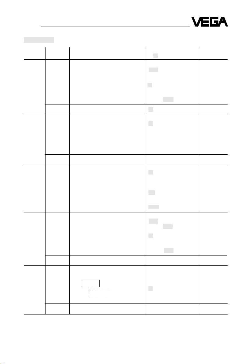
Mode listing 1

Mode-no. Mode description Parameter Page

( = factory preset)

1 - 01

1 - 02

not used ..................................................... – – – –

1 - 03 sensor type ................................................. 71 - 2 … 75 - 2

1 - 04 not used ..................................................... – – – –

1 - 05 - indication, distance in m 1 - 06 - indication, gain in dB p. 44

Working range

1 - 07 - start of working range ............................ 0 m

1 - 08 - end of working range ............................ 6 / 12 / 24 / 36 m

Product type

1 - 09 - liquids / solids ........................................ VEGASON 71 and 72 1 / 0 p. 45

VEGASON 73 … 75 1 / 0

Liquid

1 - 10 - vessel top flat / dished .......................... 1 / 0 p. 45

Solids

1 - 10 - angle of repose ..................................... 0 … 50 degrees p. 46

1 - 11 - particle size............................................ 1 … 11 mm

Sensor optimization 1, channel 1

0 - 99

0 - 01

1 - 01

2 - 01

1 - 99

MODE 0 - 99

Sensor optimization

Reset

Page 42

Sensor optimization

42 71 - 2 … 75 - 2

Mode listing 1

Sensor optimization 1, channel 1 (continuation)

Multiple echo

1 - 12 - reduction ............................................... 0.00 … 1.25 V p. 47

1 - 13 - optimization ........................................... 0.00 … 1.25 V

False echo learn

1 - 14 - indication, gain

1 - 15 - learn distance ........................................ 0,3 m … 12 / 24 / 36 m 2 m p. 48

1 - 16 - delete learn cycle .................................. 0 / 1

1 - 17 - activate learn cycle ............................... 0 / 1

Profile interpolation

1 - 18 - switched off / switched on ..................... 0 / 1 p. 49

1 - 19 Rate of product level change ..................... 0.01 … 11 cm / s (4 cm / s) p. 50

Max. gain

1 - 20 - indication, gain

1 - 21 - limitation................................................. 0.03 … 4.95 V p. 51

1 - 22 - optimization ........................................... 0.03 … 4.95 V

Measuring window

1 - 23 - switched on / switched off ..................... 1 / 0 p. 52

Fault signals

1 - 24 - switched on / switched off ..................... 0 / 1 p. 52

1 - 25 Real distance ............................................. 0,3 m … 12 / 24 / 36 m 2 m p. 53

1 - 26 not used ..................................................... – – – –

Basic adjustment (factory preset)

1 - 27 - switched off / switched on ..................... 0 / 1 p. 53

1 - 51 … 75 Service activities ........................................ PASS

1 - 99 Change

- general parameter ................................. 0

- sensor optimization 1 ............................ 1

- sensor optimization 2 ............................ 2

- linearization curve 4 .............................. 4

- linearization curve 5 .............................. 5

- linearization curve 6 .............................. 6

sensor optimization 2, channel 2 as above, however 2 - 01 … 2 - 99

Mode-no. Mode description Parameter Page

( = factory preset)

Page 43

Sensor optimization

71 - 2 … 75 - 2 43

Information for sensor optimization 1

If optimization is required, always compare the local conditions with the programmed parameters - if necessary correct or adapt.

Basic test of

Mode-no. Information Selection / measures Page

1 - 09 product type liquids or solids p. 45

1 - 10 vessel geometry vessel top flat or dished p. 45

1 - 10 solid define particle size / p. 46 1 - 11 angle of repose

1 - 19 rate of level change define in cm / sec. p. 50

False echo tests

Mode-no. Mode description Page

False echo BEFORE useful echo (output too high)

1 - 07 start of working range define p. 44

1 - 14 …17 false echo learn (activate) p. 48

1 - 18 profile interpolation activate p. 49

False echo AFTER useful echo (output too low)

1 - 08 end of working range define p. 44

1 - 12 / 13 multiple false echo reduce p. 47

1 - 21 / 22 max. gain limited p. 51

Supplementary programmings

1 - 23 measuring window switched on or off p. 52

1 - 24 false echo determine p. 52

1 - 25 real distance program p. 53

1 - 27 basic adjustment define p. 53

Above information for sensor optimization, relate to sensor 1, channel 1.

Sensor optimization for sensor 2, channel 2 as described on page 43 … 45, however mode 2 - 01 … 2 - 27.

Page 44

Working range reduction

44 71 - 2 … 75 - 2

Working range MODE 1 - 05 … 1 - 08

The working range can be limited in this mode by programming of

- start of working range and

- end of working range in case of failure. Echoes outside this limitation are ignored, e.g.

- false echoes in the narrow range

- multiple echoes by reflection in empty vessels (see programming example)

Note:

In case of multiple reflections, a limited operating range may not be sufficient. The end of working range should be programmed min. 10 % > than the max. vessel height.

min. distance (e.g. VEGASON 74 - 2)

max. vessel distance end of working range

max. distance (e.g. VEGASON 74 - 2)

Programming example:

Indication of distance in m ........................................ • can be indicated in mode 1 - 05

Indication of gain in dB ............................................. • can be indicated in mode 1 - 06

Start of working range............................................... • mode 1 - 07 is here indicated as programming

example

End of working range................................................ • select mode 1 - 08 in MODEFIELD

• program 14.00 m in PARAMETER FIELD

• then store with STO-button

0 m

Mode 07 / 08

0,8

false echo by reflections

Page 45

Adaption to the product

71 - 2 … 75 - 2 45

Product type MODE 1 - 09

The product type together with the vessel geometry can generate different reflections and therefore multiple echoes.

The available product type can be selected in this mode. With this selection the data of the factory preset of mode 1 - 10 and 1 - 11 can be activated.

The echo amplification is reduced or adapted after the measuring window.

Programming example:

Change of liquids to solids ....................................... • select mode 1 - 09 in MODEFIELD

• program figure 0 in PARAMETER FIELD

• then store with STO-button

(Requirement for page 45)

Product type ................................ Mode 1 - 09 = 1 = liquids Mode 1 - 09 = 0 = solids

Liquid Solid

vessel geometry solid features

- flat vessel top - particle size > 10 mm

- dished vessel top - angle of repose 0°

Liquid MODE 1 - 10

The vessel geometries of tank ceilings generate characteristic multiple echoes.

They can be suppressed by adaption. A flat ceiling is programmed as factory preset.

Features:

Mode 10 = 1 flat vessel top ............................... = weak tendency to multiple echoes

= 0 dished vessel top ......................... = strong tendency to multiple echoes

(parabolic effects in the top area of tank)

Programming example:

Change of flat to dished vessel top .......................... • select mode 1 - 10 in MODEFIELD

• program figure 0 in PARAMETER FIELD

• then store with STO-button

Adaption to the vessel geometry

Page 46

Adaption to the solid

46 71 - 2 … 75 - 2

Solid MODE 1 - 10 and 1 - 11

Certain characteristics can cause different multiple echoes, e.g.:

- surface structure of the solid

- type of filling / emptying

- angle of repose

- particle size of the solid.

In case the factory preset

- angle of repose 0°

- particle size > 11 mm do not ensure a reliable suppression of the multiple echoes, they can be adapted.

Min. distance e.g. VEGASON 74 - 2,

(at particle size < 5 mm)

Real echo

Multiple false echo

Max. distance (e.g. VEGASON 74 - 2)

Programming example:

Requirement: Solids activated (see page 45)

Programming the angle of repose (e.g. 30°) ............ • select mode 1 - 10 in MODEFIELD

• program angle of repose 30 degrees in PARAMETER FIELD

• then store with STO-button

Programming the particle size (e.g. 2 mm) .............. • select mode 1 - 11 in MODEFIELD

• program particle size 02 mm in PARAMETER FIELD

• then store with STO-button

0 m

1,1

Angle of repose

Page 47

Reduction of gain

71 - 2 … 75 - 2 47

Multiple false echo reduction MODE 1 - 12 and 1 - 13

Tanks with arched ceilings and therefore strong parabolic effects or silos with fine ground solids can cause strong multiple echoes.

If the measures carried out in mode 1 - 09 … 11 are not sufficient, an additional reduction by OFFSET can be carried out.

Reduction range (Offset range)

= 0.00 … 1.25

Practice values = 0.00 … 0.20

The reduction (offset) is carried out independent of the function and starts with the end of the measuring window

Programming example:

Reduction and optimization of e.g. 0,20

Reduction ................................................................. • select mode 1 - 12 in MODEFIELD

• program reduction 0.12 (V) in PARAMETER FIELD

• then store with STO-button

Optimization ............................................................. • select mode 1 - 13 in MODEFIELD

• activate optimization with MOD-button (the whole parameter indication 0,12 flashes)

• optimize with Plus-button up to e.g. 0,20 (V) (the optimization is operated in 0,01 V steps)

If during the optimization a modification to the opposite direction is required, this can be made with the minus button.

Real echo

Multiple false echo

Page 48

Storage of a false echo profile

48 71 - 2 … 75 - 2

False echo learn MODE 1 - 14 … 1 - 17

Construction details inside the vessel such as e.g.

- weldment joints

- edges

- ladders

- struts etc. create false echoes.

In a learn cycle these echoes can be determined and stored on

- location and

- strength (amplitude). In a later measuring cycle the stored false echoes

are gated out.

Requirements

- The strength (amplitude) of the useful echo must be larger in the interference position than that of the false echo.

- The vessel must be emptied to a minimum and the distance to the product must be determined, e.g. sounded.

Procedure

- program dipped value for the learn distance

- activate learn cycle With varying product surfaces the learn cycle can be repeated. The data is up-dated.

Programming example (with VEGASON 75 - 2)

Indication of gain ...................................................... • can be displayed in mode 1 - 14

Program learn distance ............................................ • select mode 1 - 15 in MODEFIELD

• program learn distance 24.00 in PARAMETER FIELD

• then store with STO-button

Activate cycle ........................................................... • select mode 1 - 17 in MODEFIELD

• select learn cycle in PARAMETER FIELD with the figure 1

• then store with STO-button, activate learn cycle During the learn cycle (approx. 3 … 4 Min.) CAL

flashes.

Delete false echo data ............................................. • the delete procedure can be triggered in mode

1–16

0 m

Real echo

False echo

sounding e.g. 24 m

Page 49

Storage of a false echo profile

71 - 2 … 75 - 2 49

Profile interpolation MODE 1 - 18

With the function "false echo learn" gaps can exist between the false echoes gated out.

With the activation of the profile interpolation, gaps smaller 3 m will be closed.

Build-up around struts, weldment joints etc. caused after the time cycle, generate additional false echoes.

Demonstration as comparison

Additional false echoes by build-up

Programming example .......................................... • select mode 1 - 18 in MODEFIELD

• program with figure 1 the profile interpolation in PARAMETER FIELD

• then store with STO-button

Profile interpolation ......................................... off .............. on

Page 50

Adaptation to filling and emptying speed

50 71 - 2 … 75 - 2

Rate of product level change MODE 1 - 19

The rate of product level change is factory set by VEGA within the adjustment range

- 0.01 … 11 cm / sec. with

- 4.00 cm / sec.

This adjustment should only be changed if this seems useful in case the actual rate of product level change exceeds the standard value.

Programming example

Change to 0,50 cm / sec. ......................................... • select mode 1 - 19 in MODEFIELD

• program 0.50 in PARAMETER FIELD

• then store with STO-button

Conversion schedule ............................................. cm / sec. m / hours

Adjustment range ........ 0,01 0,36

0,05 1,8 0,1 3,6 0,5 18,0 1,0 36,0 2,0 72,0 4,0 144,0 6,8 216,0 8,0 288,0

10,0 360,0

Page 51

Limitation of the echo gain

71 - 2 … 75 - 2 51

Max. gain MODE 1 - 20 … 1 - 22

By using the whole gain, the pulse echo measuring system tries to detect an echo. This means that in empty vessels the gain can be bigger than required for the useful echo.

This is why sound reflections are detected as false echoes. Therefore it is necessary to limit the control range of the gain.

Note:

- The limitation is adjustable from 0.03 V to

4.50 V, as optimization up to 4.95 V.

- The optimum adjustment of this mode is only possible with empty vessel.

- For orientation a d is displayed as long as an echo (false echo) is detected with actual gain.

Programming example:

Indication of echo gain ............................................. • select mode 1 - 20 in MODEFIELD

• e.g. 2.00 is indicated in the PARAMETER FIELD, i.e. a false echo is detected with a gain of

2.00 Volt

Limitation .................................................................. • select mode 1 - 21 in MODEFIELD

• program as limitation in PARAMETER FIELD e.g.

2.30

• then store with STO-button

Optimization ............................................................. • select mode 1 - 22 in MODEFIELD

• e.g. d 2.30 is displayed in the PARAMETER FIELD

• activate the optimization with MOD-button

• optimize with Plus-button the gain as long as the d extinguishes (the optimization is made in 0,02 V-steps)

If during the optimization a modification to the opposite direction is required, this can be made with the minus button.

Page 52

Supplementary optimization

52 71 - 2 … 75 - 2

Fault signal MODE 1 - 24

The fault signal is triggered when the reliability cannot be guaranteed. The reliability is calculated from the ratio between echo measurement to noise level measurement.

The fault signal can be modified as follows:

Explanation in case of failure

Fault signal off = 0 (factory preset):

- no fault signal is indicated

- the last correctly detected measured value is stored

- with the detection of new correct echo, the last stored value is cancelled and the actual one indicated

The relay and current outputs react in both cases acc. to their channel coordinations and to the failure actions adjusted in mode 0 - 93.

Fault signal on = 1:

- no fault signal is indicated

- fail safe relay de-energizes

- the failure LED of the concerned channel lights

- with the correction of a new correct echo, the feeding phase is automatically started and after it is finished, an actual measured value is indicated

Programming example

for fault signal on ...................................................... • select mode 1 - 24 in MODEFIELD

• program fault signal on 1 in PARAMETER FIELD

• then store with STO-button

Measuring window MODE 1 - 23

The measuring window must be switched off to achieve reliable measuring results in case of level changes > 10 cm / sec. or fluctuating level changes.

Attention:

When switching off the measuring window always the first large echo is detected within the working range.

Programming example .......................................... • select mode 1 - 23 in MODEFIELD

• program measuring window off 0 in PARAMETER FIELD

• then store with STO-button

Any learn cycle already activated in mode 17 is not used, however its data is not lost.

Page 53

Supplementary optimization

71 - 2 … 75 - 2 53

Basic adjustment MODE 1 - 27

All parameters, the data of which had been modified during start-up or sensor optimization, can be reset to the factory preset if necessary.

Note:

- the data of the false echo memory determined in mode 17 is not detected

- switching to of the basic adjustments triggers a new start-up condition

- the fail safe relay de-energizes

Result:

- the display indicates for approx. 3 secs. CAL (flashing)

- all modes of sensor optimization 1 or 2 are reset to factory preset (see protocol page 54)

- the respective sensor starts operating, therefore the fail safe relay de-energizes and the failure LED lights

- CAL extinguishes after approx. 3 secs. and the figures 0.000 are indicated

- this means that the basic adjustment is activated

- acc. to the time schedule a measurement is indicated or the measuring system repeats its operation (E2.01) using the basic adjustment (factory preset)

Programming example .......................................... • select mode 1 - 27 in MODEFIELD

• in PARAMETER FIELD change the figure 0 to figure 1 (prepare basic adjustment for activation)

• then store with STO-button the basic adjustment

Real distance MODE 1 - 25

As described before, all echoes within the measuring window are evaluated (useful and false echo). Therefore the measuring window can position on a false echo for different reasons. The cause is a false measurement.

In these cases an actual value can be defined by correction of the distance, i.e. by positioning the measuring window correctly and updating the measurement. To avoid repetition it is useful that the respective optimizations are carried out, e.g.

Preventive optimizations

- angle of repose adapted (mode 1 - 10)

- particle size adapted (mode 1 - 11)

- start false echo learn (mode 1 - 17)

- switch on profile interpolation (mode 1 - 18)

- adjust rate of product level change very precisely (mode 1 - 19)

Procedure

- determine the actual distance to the product surface (e.g. dip etc.).

- program this value in mode 1 - 25

With reducing level a build-up of e.g. 10 m is detected and evaluated. The actual level however is lowered to 23 m.

Programming example .......................................... • select mode 1 - 25 in MODEFIELD

• program the real distance of 23.00 (real echo) in PARAMETER FIELD

• then store with STO-button

Page 54

Supplement

54 71 - 2 … 75 - 2

Mode-no. Mode description Factory preset Sensor optimization 1 - or 2 - 123

Working range

07 - start ....................................................... 0.00 m

08 - end 71 - 2 ................................... 6.00 m

72 - 2 ................................... 12.00 m

73 - 2 ................................... 12.00 m

74 - 2 ................................... 24.00 m

75 - 2 ................................... 36.00 m

Product type

09 - liquid / solid

for VEGASON 72 .................................. 1 (liquid)

for VEGASON 73 … 75 ........................ 0 (solid)

Solid

10 - angle of repose in degrees ................... 0 degrees

11 - particle size ........................................... 11 mm

Liquid

10 - vessel top flat / dished .......................... 1 (flat)

Multiple false echo

12 - reduction in Volt .................................... 0.00

13 - optimization ........................................... 0.00

False echo learn

15 - learn distance in m ................................ 2.00

16 - delete learn cycle .................................. 0 (off)

17 - activate learn cycle ............................... 0 (off)

18 Profile interpolation .................................... 0 (off)

19 Rate of product level change in cm / sec. .. 4.00

Max. gain

21 - limitation in Volt ..................................... 0.03

22 - optimization in Volt ................................ 0.03

23 Measuring window ..................................... 1 (on)

24 Fault signal ................................................ 0 (off)

25 Real distance in m ..................................... 2.00

27 Basic adjustment ....................................... 0 (off)

Date Name

Protocol of the sensor optimization

Page 55

Supplement

71 - 2 … 75 - 2 55

Error codes

Problems during measurement or faulty adjustments during the programming are indicated on the display with a fault signal.

Fault signals are made in the measured value (mode) with channel specific indication via the respective display.

The following fixed coordination is valid:

- display 1 indicates fault signals of channel 1

- display 2 indicates fault signals of channel 2, also if the differential result has been coordinated to the respective display (mode 40).

Acc. to the table below, fault signals can cause the fail safe relay to de-energize and the failure LEDs light (channel 1 = LED 1, channel 2 = LED 2).

The current outputs as well as the switching relays react channel specific acc. to the table below or their parameter adjustment in mode 93.

After removing the failure (e.g. repair of a line break) the fault signal extinguishes automatically.

Example of a fault signal: 1 E 3 . 0 4 Fault in channel 1:

line break / temperature sensor defect

= coding of the error = error class = E = Error

Error

E3.04

- is undelayed with the switch on,

- is indicated during operation after approx. 15 secs.

error error preset fail safe relay output / code meaning mode 1 - 24 relay / -LED current output

or 2 - 24

E2.01 signal- / noise = 0

distance < 1 dB acc. to parameter adjustment

in mode 93

= 1

E2.02 echo in dead band no modification corresponds to E2.03 postoscillation influence the value for 100 %

> 1,8 m

E3.01 data loss in the no E3.02 data memory influence no modification E3.03

E3.04 line break / = 0

temperature acc. to parameter adjustment sensor defect in mode 93

= 1

ERR parameter range no

exceeded by influence no modification adjustment

Page 56

VEGA Grieshaber KG

Electronic level measurement Am Hohenstein 113 Postfach 11 42 D-77757 Schiltach Phone 0 78 36/50-0 Fax 0 78 36/50-201

2.14 655 / April '94Technical data subject to alterations

VEGA SON71 User Manual

Specifications and Main Features

Frequently Asked Questions

User Manual