UVP Doc-It Life Science User Manual

Doc-It® Life Science Software

Installation and User Instructions

Doc-It®LS Image Acquisition Software Doc-It®LS Image Analysis Software

UVP, LLC Ultra-Violet Products Ltd

2066 W 11th Street, Upland, CA 91786 Unit 1, Trinity Hall Farm Estate Tel: (800) 452-6788 / (909) 946-3197 Nuffield Road, Cambridge CB4 1TG UK Fax: (909) 946-3597 Tel: +44(0)1223-420022 / Fax: +44(0)1223-420561 Email: info@uvp.com Email: uvp@uvp.co.uk

Web site: uvp.com

81-0328-01 Rev B

Table of Contents

Introduction.................................................................................................................................................... 1

Welcome .................................................................................................................................................... 1

Minimum System Requirements ................................................................................................................ 2

Registering and Activating the Software .................................................................................................... 2

Single-User License ................................................................................................................................... 4

User Administration .................................................................................................................................... 4

Technical Support ...................................................................................................................................... 7

License Agreement .................................................................................................................................... 8

Navigating the Software .............................................................................................................................. 10

Main Window ........................................................................................................................................... 10

Menus ...................................................................................................................................................... 10

Toolbars ................................................................................................................................................... 11

Image Windows ....................................................................................................................................... 13

Using Plug-In Modules ................................................................................................................................ 15

Overview .................................................................................................................................................. 15

Positioning Plug-in Modules .................................................................................................................... 16

Histogram Controls .................................................................................................................................. 17

Digital Video Player .................................................................................................................................. 17

Image Controls Plug-In ............................................................................................................................ 21

3D Plots ................................................................................................................................................... 23

FTP Transfer ............................................................................................................................................ 24

Log Viewer ............................................................................................................................................... 24

Zoom/Pan ................................................................................................................................................ 24

Camera Plug-In ........................................................................................................................................... 27

Capturing Images ........................................................................................................................................ 30

Creating Templates ..................................................................................................................................... 31

Set-Up Templates .................................................................................................................................... 31

Edit and Delete Templates ...................................................................................................................... 31

Set-Up Canon Capture Templates .......................................................................................................... 31

Creating Colony Templates ..................................................................................................................... 32

Deleting Colony Counting Templates ...................................................................................................... 33

Editing Images ............................................................................................................................................ 34

Overview .................................................................................................................................................. 34

Copy ......................................................................................................................................................... 34

Paste ........................................................................................................................................................ 35

Undo and Redo ........................................................................................................................................ 35

Using the Region of Interest Tools .......................................................................................................... 36

Using Image Filters ..................................................................................................................................... 37

Overview .................................................................................................................................................. 37

Filter Navigation ....................................................................................................................................... 37

Filter Menu ............................................................................................................................................... 37

Filter Plugins ............................................................................................................................................ 37

Background Filter ..................................................................................................................................... 38

Burn Changes to a New Image ................................................................................................................ 39

Convert Image ......................................................................................................................................... 39

Duplicating Images .................................................................................................................................. 39

Flip Image ................................................................................................................................................ 39

Image Enhancement Filters ..................................................................................................................... 40

Image History ........................................................................................................................................... 41

Measurement Tools ................................................................................................................................. 42

Merging Two Images ............................................................................................................................... 43

Obtaining Image Information ................................................................................................................... 44

Pseudocolor ............................................................................................................................................. 45

Reduce Image to Mono............................................................................................................................ 46

Resize Image ........................................................................................................................................... 46

Rotate and Align Image ........................................................................................................................... 47

Rulers ....................................................................................................................................................... 48

Scanning Images ..................................................................................................................................... 48

Spatial Calibration .................................................................................................................................... 49

Annotations ................................................................................................................................................. 51

Overview .................................................................................................................................................. 51

Types Of Annotation ................................................................................................................................ 51

Viewing And Hiding Annotations .............................................................................................................. 52

Synchronize Size with Image Zoom ........................................................................................................ 52

New Annotation Window .......................................................................................................................... 52

To Edit the Text of a Text Annotation ...................................................................................................... 52

Selecting Annotations .............................................................................................................................. 53

Moving And Resizing Annotations ........................................................................................................... 53

Formatting Annotations ............................................................................................................................ 55

Deleting Annotations ................................................................................................................................ 55

Creating Annotations ............................................................................................................................... 56

Loading and Saving Images ....................................................................................................................... 57

Loading Images ....................................................................................................................................... 57

Saving Images ......................................................................................................................................... 57

Burn in Changes to a New Image ............................................................................................................ 58

Image File Types ..................................................................................................................................... 58

Performing 1D Analysis ............................................................................................................................... 60

Navigating 1D Analysis ............................................................................................................................ 60

1D Analysis Plugin Module ...................................................................................................................... 60

1D Analysis Context Menu Commands ................................................................................................... 62

Finding Lanes and Bands ........................................................................................................................ 62

1D Analysis Image Window Features ...................................................................................................... 64

1D Analysis Settings ................................................................................................................................ 65

Manually Modifying Lanes and Bands ..................................................................................................... 65

Lane and Band Information ..................................................................................................................... 68

Lane Profile Graph ................................................................................................................................... 69

Viewing and Printing 1D Gel Analysis ..................................................................................................... 71

Viewing Data Explorer Results ................................................................................................................ 72

Printing Data Explorer Tabular Reports ................................................................................................... 75

Performing Concentration Calibrations .................................................................................................... 77

Performing Molecular Weight Calibration ................................................................................................ 82

Retardation factor (Rf) Lines .................................................................................................................... 86

Performing Dendrogram Analysis ............................................................................................................ 87

Performing Colony Counting ....................................................................................................................... 91

Colony Count Module .............................................................................................................................. 91

Preference Settings for Colony Counting ................................................................................................ 92

Automatic Counting .................................................................................................................................. 93

Manual Counting ...................................................................................................................................... 93

Manual Counting Step 1: Select Classes ................................................................................................ 94

Manual Counting Step 2: Finish ............................................................................................................... 94

Edit Colonies ............................................................................................................................................ 95

Add Colonies ............................................................................................................................................ 95

Delete Colonies ........................................................................................................................................ 96

Split Colonies ........................................................................................................................................... 96

Merging Colonies ..................................................................................................................................... 97

User Defined Template Counting ............................................................................................................ 97

Spiral Counting ........................................................................................................................................ 97

Zone Analysis .......................................................................................................................................... 98

Renumbering Colony/Zone Values .......................................................................................................... 99

Reporting Functions ................................................................................................................................. 99

Classes .................................................................................................................................................... 99

Statistics ................................................................................................................................................. 100

Distribution ............................................................................................................................................. 100

Export and Print Colony Results ............................................................................................................ 100

Printing Reports and Images .................................................................................................................... 101

File Print Command ............................................................................................................................... 101

iii

Printing Image History............................................................................................................................ 101

Print ........................................................................................................................................................ 102

Supporting 21 CFR Part 11 Compliance ................................................................................................... 103

Purpose .................................................................................................................................................. 103

Features ................................................................................................................................................. 103

Usage ..................................................................................................................................................... 103

Glossary .................................................................................................................................................... 105

Introduction

Welcome

Life Science (LS) software from UVP lets users acquire, enhance, and analyze images in a simple and efficient way.

The software is designed to image electrophoresis gels (DNA, RNA, Protein), blots, membranes, plates, plants, and animals. Once the image has been captured with an application-specific camera, it can be saved for record keeping purposes, manipulated for analysis, and annotated to point out key features.

If a software function is grayed out, the function is not available with the version of software loaded on the user’s computer.

Getting Started

Minimum System Requirements Registering and Activating the Software

Capturing Images

Cameras

Performing Analysis Functions on Images

1D Analysis Molecular Weight Calibrations Concentration Calibrations Dendrogram Analysis Counting Colonies

Minimum System Requirements

Windows XP Professional with Service Pack-2 or higher (32 bit only), Vista (32 bit only), or

Windows 7 (32 bit only)

Internet Explorer 6.0 or higher [To determine the version of Internet Explorer, open Internet

Explorer and click on Help > About] Intel Pentium Processor or equivalent, 1.6 GHz or higher 1 GB of RAM or greater (2 GB recommended) 200 MB of available hard disk space for the program, more for data To avail the functionality of 21 CFR Part 11, the partition must be formatted with NTFS. CD-ROM drive Color monitor, supporting at least 1024 x 768 resolution and 16-bit or better colors; 24-bit or 32-

bit color is strongly recommended

Registering and Activating the Software

Overview

Introduction

Single-User License User Administration

Overview

Use of LS software requires activation of a security code from UVP. Registration and activation of the software can be accomplished by phone, email or by the Internet. Two types of licenses are available, single-user or network-user with a five-user license. Additional licenses are available.

Registering the Software

Activate the software by entering an activation code provided by UVP in order to gain full access rights to the software.

Once the LS software is installed, it will operate in full-future trial mode for 14 days. Within the 14-day trial mode, the LS software must be registered with UVP. Otherwise the software will only operate in demonstration mode after the 14-day trail period. The demonstration mode limits the software to only open and use the demonstration images provided by UVP.

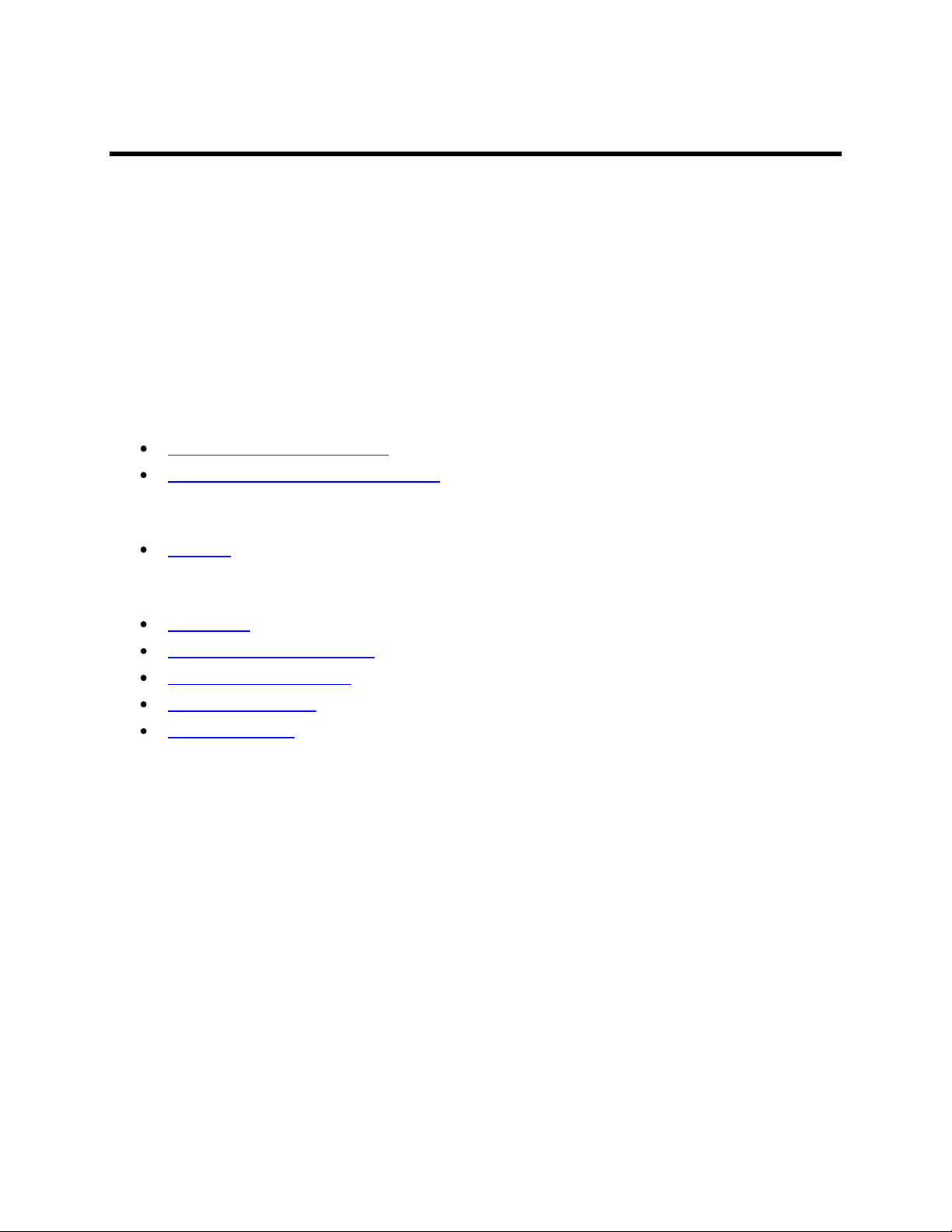
The License Wizard window will appear. There are three ways to retrieve an activation code: phone, email or Internet and selecting one of the options from the License Wizard window.

On the Fly Activation: Choose this option to activate the software immediately through the

Internet. Already Have an Activation ID: This option is useful when reloading (or upgrading) the software

after receiving an initial activation code. Offline Activation: This option is used if the computer is not connected to the Internet. This

allows the user to obtain the activation code and enter it at another time

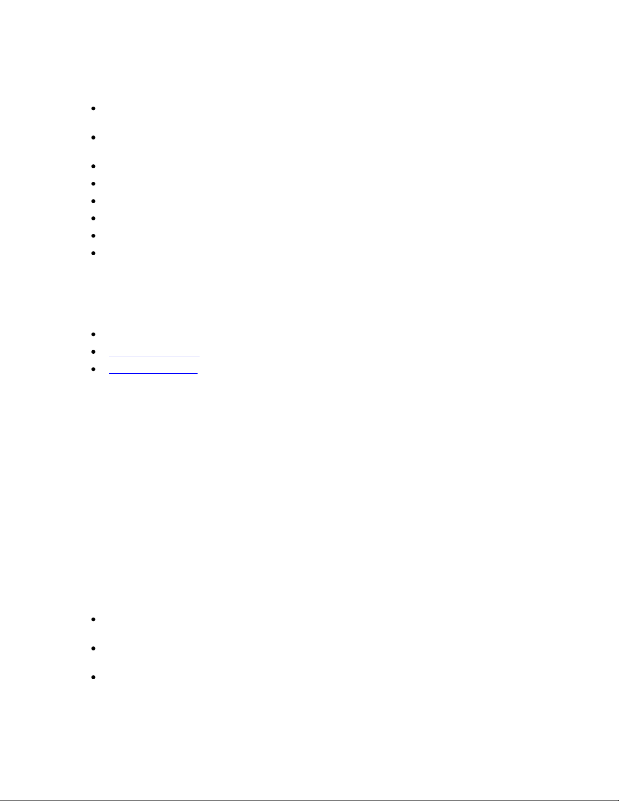
On the Fly Activation

To immediately activate the software through the Internet:

Choose On the fly activation. If the computer is not connected to the Internet, follow the

instructions for Offline activation or call UVP to register the software.

Introduction

Click Next to continue. Complete all required information on the form.

Fill out the Serial Number located on the CD. The number should be four sets of six numbers. Click the Get Activation No. button and then click onto Activate when the Activation Number

appears in the box.

Already Have an Activation ID

Select Already have an activation ID from the buttons. This activation function is useful when

reloading the software after receiving an initial activation code. Click Next to continue. Click the link provided and complete the form to obtain instructions. Click Finish.

Introduction

Offline Activation

Select Offline Activation if the computer is not connected to the Internet. This allows the user to

obtain the activation code and enter it at another time. Click Next to continue. Click the link provided and complete the form to obtain instructions. Click Finish.

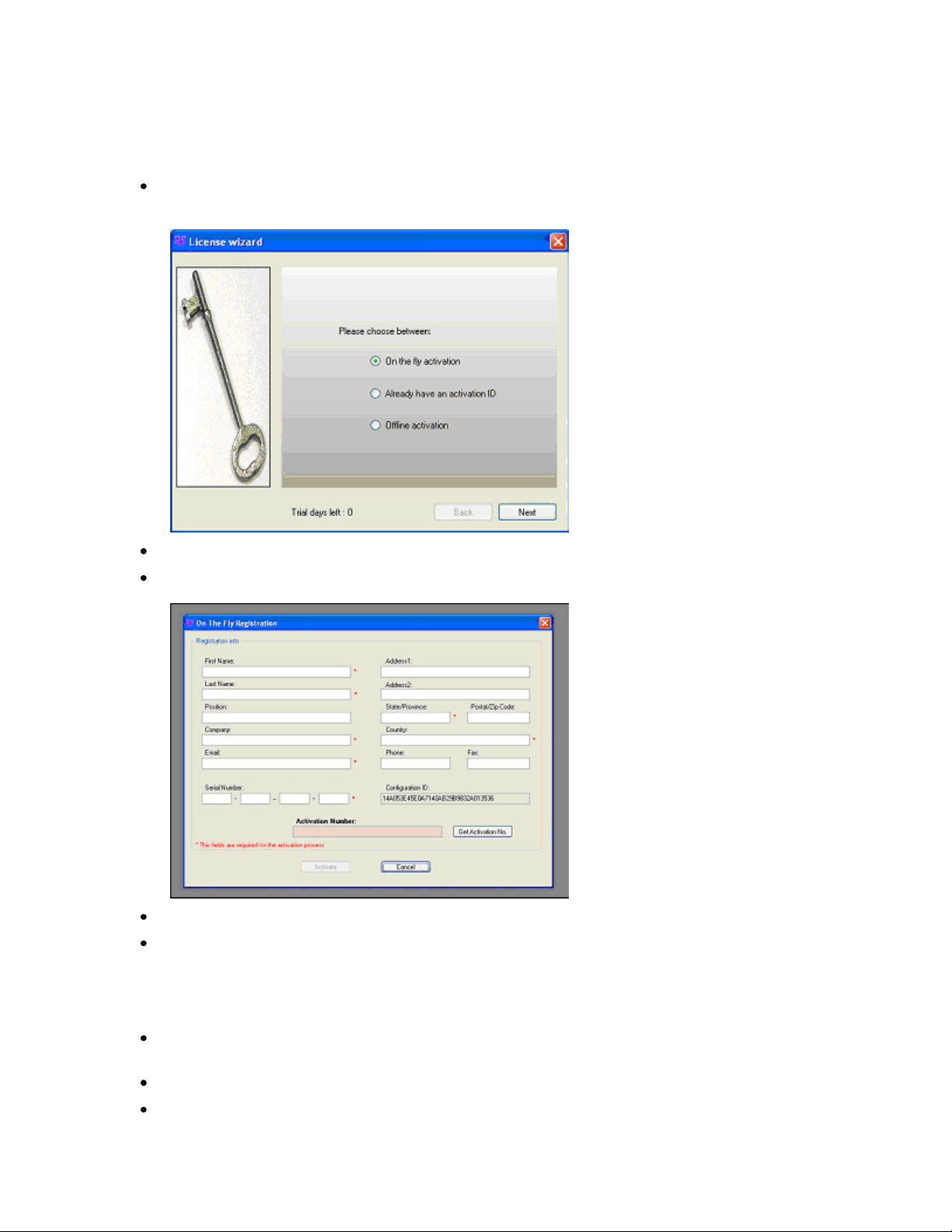
Single-User License

Single-user license allows the software to be used on a single computer. A Welcome to the Licensing Wizard window will appear. Select the Single client access license option,

and select Next.

User Administration

Secure User Accounts Usernames and Passwords User Rights

Secure User Accounts

The concept of User Accounts for individual users is central to the software by providing security of user s data from being tampered with by other users, accidentally or otherwise.

This system of usernames and passwords is separate from the one that is used to login to the

Column Heading

Description

User Name

Unique Identification name for a particular user. This could be a name or a word that makes it easier to identify the user.

Date Created

Date the user name was created.

Last Login

Date of last login.

Number of times the user has logged in.

Idle Time Lock

Indicates the maximum idle time. To change the idle time, click Tasks > Set Idle Time. Zero means no idle time.

Password Expiration Date

Date the password expires.

View

Enables user to view images. To change this setting, click Tasks > Edit Rights. Click or unclick the View option.

Change

Enables user to change images. To change this setting, click Tasks > Edit Rights. Click or unclick the Change option.

Has Admin. Rights

Gives user administration permissions. To change this setting, click Tasks > Edit Rights. Click or unclick the Has Administration Rights option.

computer. Setting up user accounts is mandatory if support for CFR 21 Part 11 is required from the

software. If individual accounts are not required, create just one account for all users and give full

permissions to that account.

Enable secure user accounts

Request a System Administrator to log into the Windows computer. Navigate to C:\Documents and Settings\All Users Locate the Application Data folder. f the Application Data folder is not present in the All Users window, go to the Tools menu and

select Folder Options. A Folder Options window appears. On the View tab, select Show hidden files and folders.

Select Apply then OK. Go to the UVPSettings folder inside the Application Data folder. Have the System Administrator set Read and Write permissions for either the UVPSettings

folder, or for each file within the folder (depending on the Network Security Policy where the LS

software will reside).

Introduction

User Administration History Definitions

The description of the settings for each column of the History section is shown below. To see all of the columns in History, move the scroll bar to right.

Usernames and Passwords

Start the software. It will bring up a Login window. The administrator user name will show.

Enter a password. On initial installation, a screen will pop up to request a password and

password confirmation. A password is required. Click Login.

Adding a New User

From the menus, click Tools > User Administration to open the User Administration window. Click the New User button, type in the user name and password. Type in the new user name and password. Each time the new user logs in, use that new user

name and password.

Editing a User

Edit the User by highlighting the user name in the User Administration window. Click the Tasks > Edit Rights and select from the Define User Permissions screen to allow

users to view images, modify images, change templates, or assign administrative rights. Click OK when changes to the user are complete.

Introduction

Changing a Password or Other Settings

To change a password, from the menu go to Tools > User Administration to open the User

Administration window.

Click on the appropriate user to change. Select the Tasks > Reset Password and enter the new password. Enter the password again to

confirm the change. Click OK. The change in password will be noted in the User Administration > History box.

Deactivating/Reactivating a User

From the menu, select Tools > User Administration to open the User Administration window. Select that user name and click Tasks > Deactivate. A red X will indicate the user is deactivated.

To reactivate, click Tasks > Activate. Click OK to close the window.

NOTE: Never disable the Administration Account.

Viewing the Login History of a User

Select a user name in the User Administration table. The lower half of the window displays the

Introduction

Install

Un-Install

Open and Run

User Administration

Use the Camera

Restricted

X* X

Standard/Power

X* X

Admin

X X X X X

X = Supported rights.

Note that even though a user may be able to do things with the software which are outside of this matrix, UVP neither recommends it, nor supports it. For example, the user may try (successfully or otherwise) to uninstall the software as a Power User, but UVP does not provide support for problems arising during or due to that action.

Users Rights

Depending on the privileges for the user that has logged onto windows, the following rights are available to that user for the software:

Technical Support

UVP offers expert technical support on all of our products. If there are questions about the product s use, operation or repair, please contact our offices at the locations below.

If located in North America, South America, East Asia or Australia:

Call (800) 452-6788 or (909) 946-3197, and ask for Technical Support during regular business

days, between 7:00 am and 5:00 pm, PST. E-mail your message to: info@uvp.com or techsupport@uvp.com Fax Technical Support at (909) 946-3597 Write to: UVP, LLC 2066 W. 11th Street, Upland, CA 91786 USA

If located in Europe, Africa, the Middle East or Western Asia:

Call +44(0) 1223-420022, and ask for Customer Service during regular business days between

8:30 am and 5:30 pm. E-mail your message to: uvp@uvp.co.uk Fax Customer Service at +44(0) 1223-420561 Write to: Ultra-Violet Products Ltd. Unit 1, Trinity Hall Farm Estate, Nuffield Road, Cambridge

CB4 1TG UK

Introduction

License Agreement

End User License Agreement

PLEASE READ THE FOLLOWING AGREEMENT CAREFULLY

This Agreement is between UVP, LLC of 2066 West 11th Street, Upland, California 91786 (hereinafter "Licensor") and the end user of UVP software (hereinafter "Licensee").

Licensor has developed and offers to Licensee on a non-exclusive basis pursuant to the terms and conditions set forth hereinafter, the following software, including related copyrighted instructional materials, (collectively referred to hereafter as "The Software"):

Doc-It LS Software

The terms of this Agreement apply without regard for the method by which the Software is acquired by Licensee. While the most common medium for acquiring the Software from Licensor is by CD-ROM, the Software may, in some instances, be acquired by download; from a Licensor thumb drive acquired from Licensor; from a CD ROM acquired from Licensor from a network location; or may be pre-installed on the Licensee s computer.

By using the Software, you are agreeing to be bound by all terms of this License. If you do not agree to the terms of the License, you are not authorized to use the Software in any manner.

License

In consideration of payment of the License fee, which is a portion of the price you paid, the software, including any images incorporated in or generated by the software, and data accompanying this License and related documentation are licensed (not sold) to you by Licensor. Licensor does not transfer title to the Software to you; this License shall not be considered a "sale" of the software and Licensor retains full and complete title to the Software and all intellectual and industrial property rights therein. It is to be understood that this non-exclusive and personal License only gives you the right to use and display the software. You must treat the software like any other copyrighted material. You may not copy the Software or the written material accompanying the software without the express written consent of Licensor.

Restrictions

The Software contains copyrighted materials, trade secrets, and other proprietary material. You may not re-sell, decompile, reverse engineer, disassemble or otherwise reduce the Software to a humanperceivable form. Except as provided for in this License, you may not copy, modify, network, rent, lease, or otherwise distribute the Software; nor can you make the Software available by "bulletin boards", on-line services, remote dial-in, or network or telecommunications links of any kind; nor can you create derivative works or any other works that are based upon or derived from the Software in whole or in part. You may not transfer the license rights to the Software to another party.

Termination

This License is effective until terminated by either party. You may terminate this License at any time by returning the Software to Licensor or destroying any permanent form of the software and all related documentation and all copies and installations thereof, whether made under the terms of this License or otherwise. This License will terminate immediately without notice from Licensor if you fail to comply with any provision of this License. Upon termination, you must destroy or return to Licensor any permanent form of the software and related documentation.

Introduction

Limited Warranty and Disclaimer

Licensor warrants the software and related documentation to be free from defects in materials and workmanship, under normal use for a period of ninety (90) days from the date of purchase as evidenced by a copy of the sales receipt or packing slip. Licensor s entire liability and licensee s exclusive remedy

will be replacement of the defective software and related documentation or refund of the purchase price (at licensor s election) upon return of the software and related documentation to licensor with a copy of

proof of purchase. This warranty gives you specific legal rights and you may also have other rights which vary from jurisdiction to jurisdiction. You expressly acknowledge and agree that use of the software is at your sole risk after the ninety (90) days. The software and related documentation are provided without warranties and/or conditions of any kind either express or implied, except as provided above. Licensor expressly disclaims all other warranties and/or conditions, express or implied, with respect to software and related documentation including, but not limited to, the implied warranties and/or conditions of merchantability and fitness for a particular purpose. Licensor does not warrant that the functions contained in the software will be uninterrupted or error-free, or that defects in the software will be corrected after the ninety (90) days. Furthermore, after the ninety (90) days, licensor does not warrant or make any representation regarding the use or the results of the use of the software and related documentation in terms of their correctness, accuracy, reliability, or otherwise. The limitations of liabilities described in this section also apply to the third party suppliers of materials used in the software. No oral or written information or advice by licensor or by representatives of licensor shall create warranties, and/or conditions, or in any way increase the scope of this limited warranty. Licensee assumes the entire cost of all necessary servicing, repair or correction after the ninety (90) days. Some jurisdictions do not allow the exclusion of implied warranties, so the above exclusion may not apply to you.

Limitation of Liability

Under no circumstances, including negligence, shall licensor be liable for any special or consequential damages that result from the use of, or the inability to use, the software or related documentation, even if licensor or authorized representative of licensor has been advised of the possibility of such damages. Some jurisdictions do not allow the limitation or exclusion or liability or consequential damages, so the above limitations or exclusion may not apply to you. In no event shall licensor s total liability to you for all

damages, losses, and causes of action (whether in contract, tort (including negligence) or otherwise) exceed the amount paid by you for the software.

Governing Law and Severability

This License shall be governed by and construed in accordance with the laws of the State of California, without giving effect to any principles of conflicts of law. Any actions, suits or proceedings instituted in connection with this License, the Software and/or related documentation shall be instituted and maintained exclusively in the Superior Court for the State of California, County of Los Angeles, or in the United States District Court for the Central District of California. By entering this License you hereby consent to the venue and jurisdiction of the aforesaid courts. If any provision of this license shall be unlawful, void, or for any reason unenforceable, then that provision shall be deemed severable from this License and shall not affect the validity and enforceability of any remaining provision. This is the entire agreement between the parties relating to the subject matter herein and shall not be modified except in writing, signed by both parties.

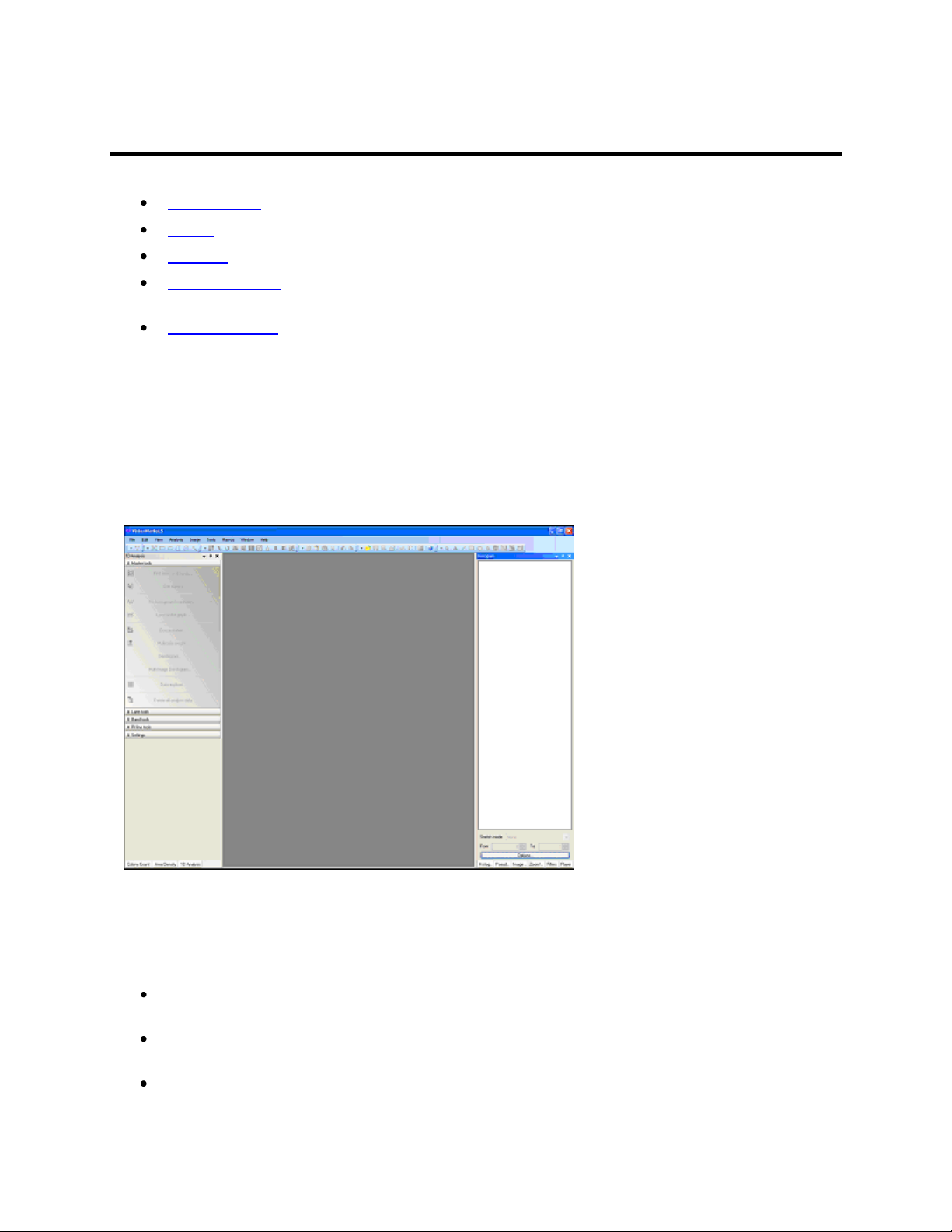
Navigating the Software

Main Window - Shows the full software screen Menus - Discusses the menus available Toolbars - Discusses the tollbars and the ability to rearrange the tool buttons Plug-In Modules - Several plug-in modules are provided as user-friendly interfaces for specific

software tasks; this section discusses the various modules and the ability to position the modules

Image Windows - Discusses the use of image windows in the workspace

Main Window

After the LS software is opened for the first time, the screen will look similar to the one shown below. The LS Main Window contains the application's menu bar, toolbars, image windows, plug-in modules and status bar. Some parts of the window, such as the toolbars, plug-in modules and status bar, can be hidden or shown if preferred.

Menus

LS Software offers the following menus:

File Menu: Contains commands to load and to save files, to select profiles, adjust preferences

and to print reports. Edit Menu: Contains the Undo/Redo commands and the clipboard commands: Cut, Copy,

Paste, Paste Special and Paste Special Options, plus the Crop function. View Menu: Contains commands that show and hide various main-window features and

commands that affect how the current sub window is displayed.

Navigating the Software

NOTE: Although most commands appear on the menus, some features are only available through the Plug-in Modules. If the Plug-in Modules are hidden, they can be shown by selecting the modules from View > Plug-ins whenever needed.

Analysis Menu: Contains modules to perform Colony Counting, 1D Analysis and Area Density. Tools Menu: Contains a list of the tools to enhance the image or software environment including

seeing Loaded Plug-ins, User Configuration, pre-configured image Reports, plus Region of

Interest, Spatial Calibration and Annotation tools. Macros Menu: Contains commands to work with Macros. A Macro is a collection of commands

that can be saved and replayed with special user-defined keys. Window Menu: Contains commands to organize Image windows. Shows the arrangement of the

image window and shows the name of the images currently open. Help Menu: Contains access to the software help, user license wizard and software version.

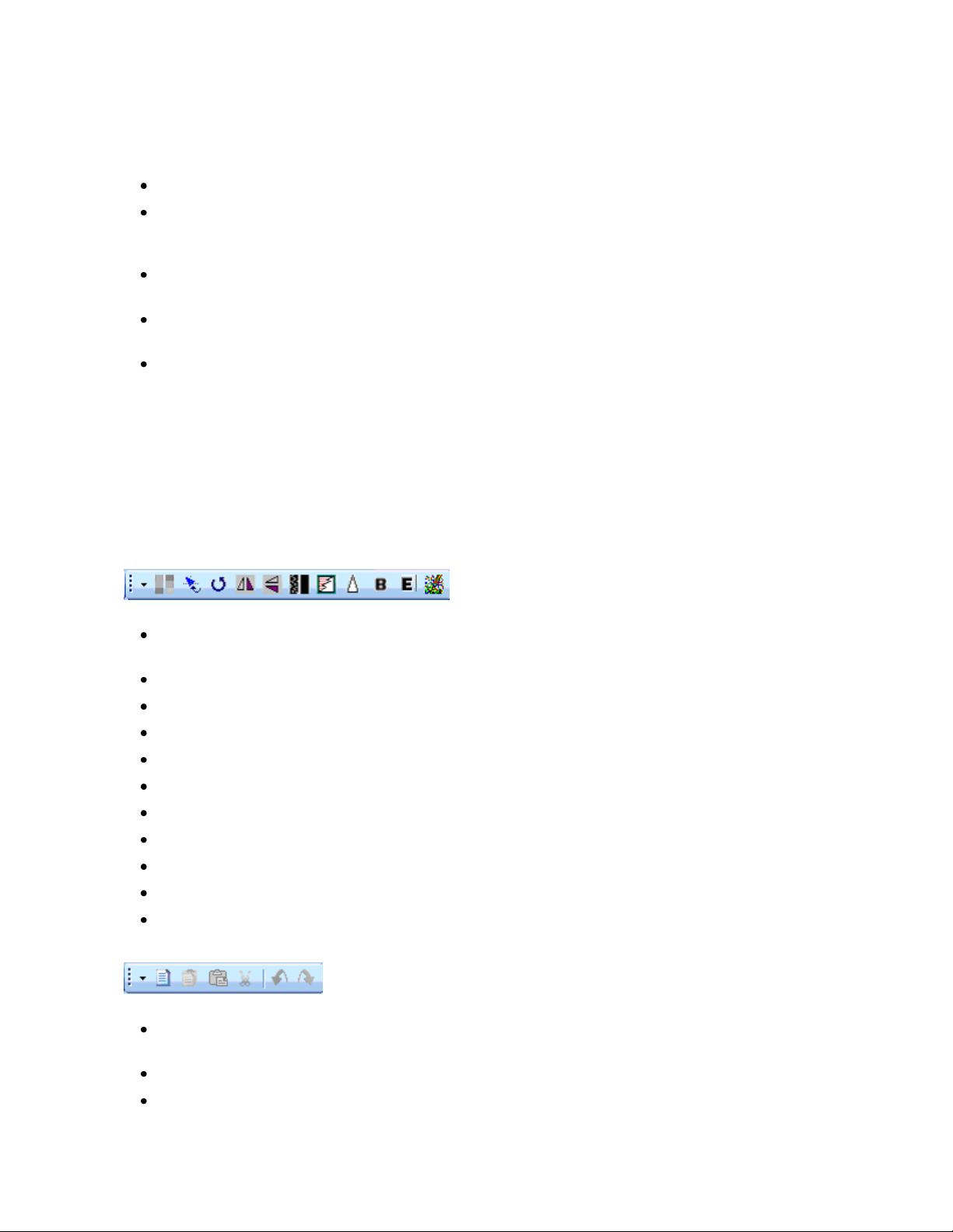
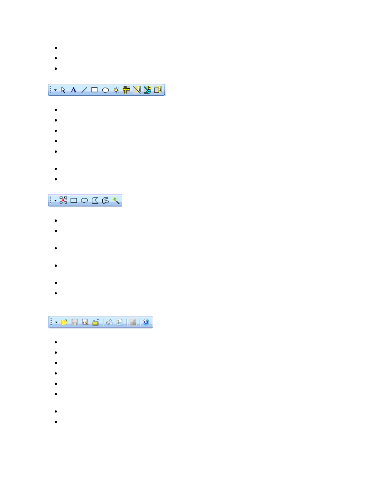
Toolbars

The toolbars in LS allow the user to select most commands with a single button click. The toolbars are customizable, so the user can include the commands used most and remove commands rarely used.

Toolbar Buttons

Reduce to Mono: Converts the image to a single-channel (monochrome) image from a multi-

channel (color) image Align: Aligns the image to a grid Rotate: Brings up the dialog box to rotate image by a specific degree or by manual rotation Flip Horizontal: Flips image horizontally Flip Vertical: Flips image vertically Despeckle: Applies the despeckle filter to the image Remove Noise: Applies the remove noise filter to the image Sharpen: Applies the sharpen filter to the image Blur: Applies the blur filter to the image Emboss: Embosses the image with selection of the direction of the emboss filter Starfield Subtraction: Applies the starfield subtraction filter to the image

Copy: Copies selected text, selected portions of the current image or the entire image to the

clipboard Paste: Pastes the current clipboard item onto the screen Paste Special: Pastes an overlay of the current item in the clipboard

Navigating the Software

Cut: Cuts a specific area Undo: Reverses the last command Redo: Repeats the last command

Arrow: Selects an annotation to edit Text Tool: Text annotation Line, Rectangle, Ellipse and Highlighter Tools: Annotation tools Define Image Scale: Allows users to set the scale for images Measure Length: Measures the distance between any two points on the image, units depend on

spatial calibration Measure Angle: Measures an angle Measure Area: Measures an area on the image

New ROI: Removes the active Area of Interest and prepares for a new one of the current type Rectangular ROI: Changes the current mouse tool to the select Rectangular Area of Interest and

brings up one if already present on the current image Elliptical ROI: Changes the current mouse tool to the select Elliptical Area of Interest and brings

up one if already present on the current image Polygonal ROI: Changes the current mouse tool to the select Polygonal Area of Interest and

brings up one if already present on the current image Freeform ROI: Changes the current mouse tool to the select a user defined Area of Interest Magic Wand ROI: Selects a consistently colored area (for example, a red flower) without having

to trace its outline

Open: Opens an image file on disk Save: Saves the current image to disk Save As: Saves the current image to a different name Close: Closes the file Print: Prints the current image Preferences: Opens the preferences window to set defaults in the following tabs: Main Settings,

Log Settings, 1D Analysis, Colony Count settings External Application: Launches a Qwik-Link external application selected in Preferences Exit: Closes the software program

Navigating the Software

Rearranging Toolbars

The order of the individual toolbar sections can be rearranged by placing the mouse arrow over the dotted line at the edge of each toolbar section and moving the toolbar. The default position of the toolbars is located horizontally below the menus. The toolbars may be moved to the bottom of the screen or vertically on the left or right side. Each section can be deleted or added back by clicking View > Toolbars and select the toolbars to display on the screen.

Image Windows

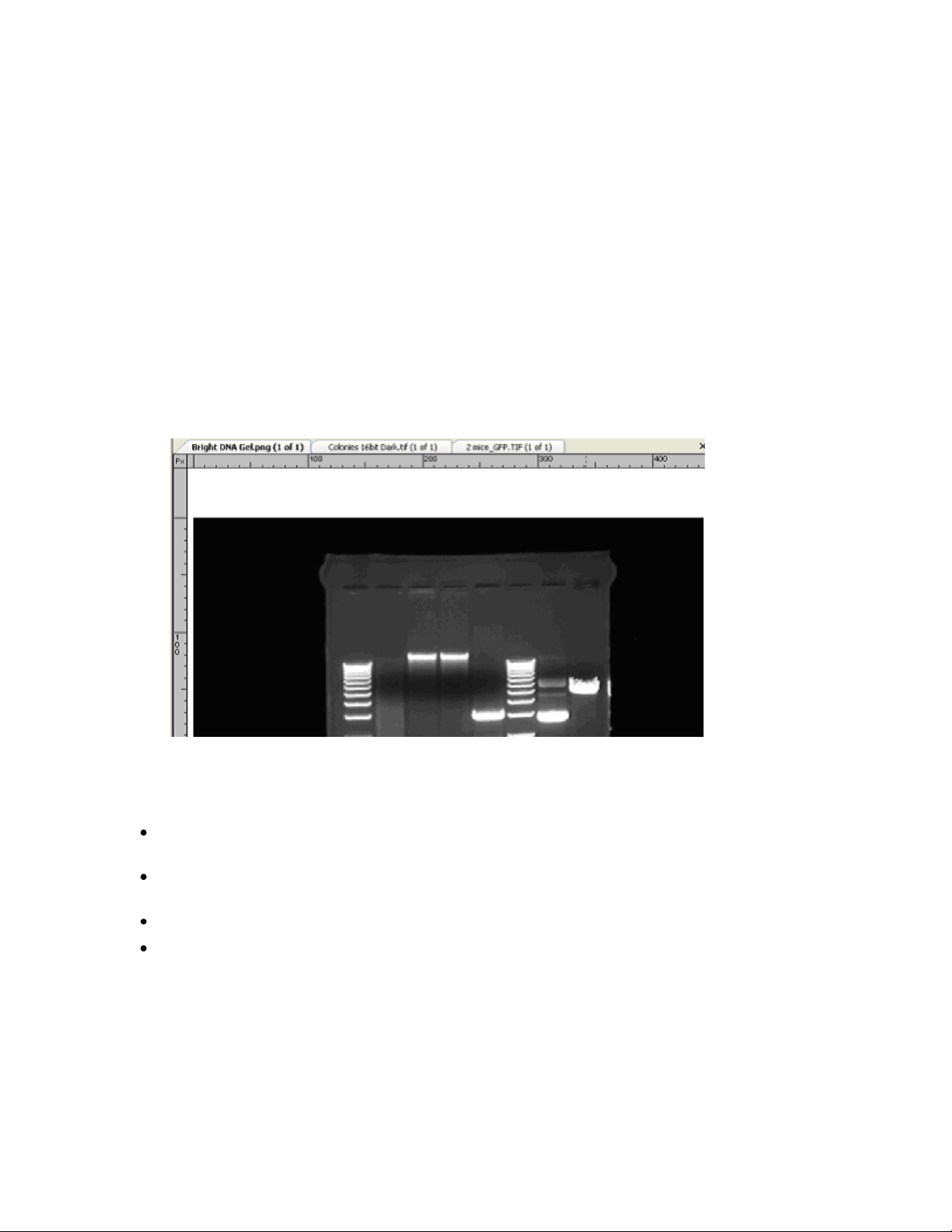
Each open image in LS workspace will appear in a separate Image Window. Several Image Windows can be opened at one time. The window below shows several images open, layered with tabs (tabbed interface turned ON in Preferences) for selection of images.

Organizing Image Windows

Images can be visible in the workspace area with either tabbed layout, shown above or cascaded images.

To change from tabbed layout to cascaded layout, on the menu, go to File > Preferences > Main

Settings and uncheck the Tabbed Interface checkbox. To bring an Image window to the forefront, either click on the window's title bar or find and select

the image's filename from the list in the Windows menu. To close an image window, click onto the X next to the image tabs. To resize a Cascaded Image window, drag the lower right corner (or an edge) to the desired size.

Information Provided by the Image Window

Besides displaying an image, the Image tab includes the filename of the image. A caption of "Untitled" means that the image has not been saved.

Navigating the Software

Showing the Image in Actual Size

To show the image in actual size (no scaling), choose View > Zoom. Set the zoom factor to 100%. Or click the right mouse button on the image and select View Original Size. Images taken at high resolution will look large on the screen.

Fitting the Image to the Window

To show the entire image in the window (scaled up or down as required to make it fit), click the right mouse button and click View Best Fit.

Context Menu Commands

A context (shortcut) menu appears when the user clicks on the image itself with the right mouse button. It is a shortcut menu that lets the user sidestep the MENUS OR TOOLBARS. Once brought up, treat it as a regular menu by selecting features from the list.

Click on the image with the right mouse button, a menu with the following commands opens:

Copy Paste Paste Special Print Selection View Best Fit View Original Size Image Information

TIP: Both the View Best Fit and View Original Size commands are also available from a shortcut menu on the Image window itself. The shortcut menu can be displayed by right clicking on the image.

Status Bar

The Status Bar shows the User Name (Profile), current mouse position in an image, the intensity of the image at that position and status messages during operations. Current date and time is display in the right corner.

The mouse position (POS) is displayed in pixels (X and Y). The Intensity is displayed as a single value if the image is monochrome and has three values (Red, Green and Blue) if the image is colored. In both cases, the value is reported as a percentage value of the maximum intensity. The ROI (Region of Interest), date, and time is also reported.

Using Plug-In Modules

Overview

The plug-in modules in LS allow the user to position modules on the work area for easy access to the plug-in functions. Position of the modules is customizable, so plug-ins can be organized to include the plug-ins used most and remove plug-ins rarely used.

To open the plug-in modules, select View > Plugins and select the plug-in to appear in the LS software workspace.

The plugins automatically loaded on the left side of the screen are Colony Count, Area Density, 1D Analysis. The plug-ins loaded on the right side of the screen are Histogram, Pseudocolors, Image controls, Zoom/Pan, Filters, and Player.

Link below for information on using specific plug-in modules:

Cameras Log Viewer Digital Video Player 3D Plot Zoom/Pan Image Controls Filters Pseudocolors Histogram Controls File transfer protocol 1D Analysis Counting Colonies

Using the Plug-in Modules

The LS software plug-in modules are essentially tool boxes for many of the commonly used features. Plug-in modules open function-specific windows that can be viewed and placed in virtually any position on the screen. To open the plug-in modules, select View > Plugins and select the plug-in to appear in the LS software workspace.

The plugins automatically loaded on the left side of the screen are Colony Count and 1D Analysis. The plugins loaded on the right side of the screen are Histogram, Pseudocolors, Image controls, Zoom/Pan, Filters, and Player.

Using Plug-In Modules

Positioning Plug-in Modules

Rearranging Plug-in Modules

Plug-in Modules can positioned anywhere on the screen. Plug-ins can be docked, hidden, and floating.

Dockable: Locks the module in a specific position. Hide: Closes the module. To reopen, go to View > Plugins and select the plug-in module. Floating: Allows module to be moved around on the screen. To move a module, click the top bar

of the module and, while holding down the left mouse button, drag the module to the desired

location. Arrows will display. Move the module to one of the arrows to dock the module. Auto Hide: Automatically hides the module when not in use. These tabs will be displayed in the

same order as they were selected to Auto Hide. To show the full module, roll the mouse over the

tab. To disable the auto hide function, unclick Auto Hide from the module drop down menu or

click the pushpin icon.

Moving a Floating Plug-in Module

When a plug-in module is floating, it can be docked to the top, bottom, left or right on the workspace. A floating plug-in module can be placed into another plug-in module s window.

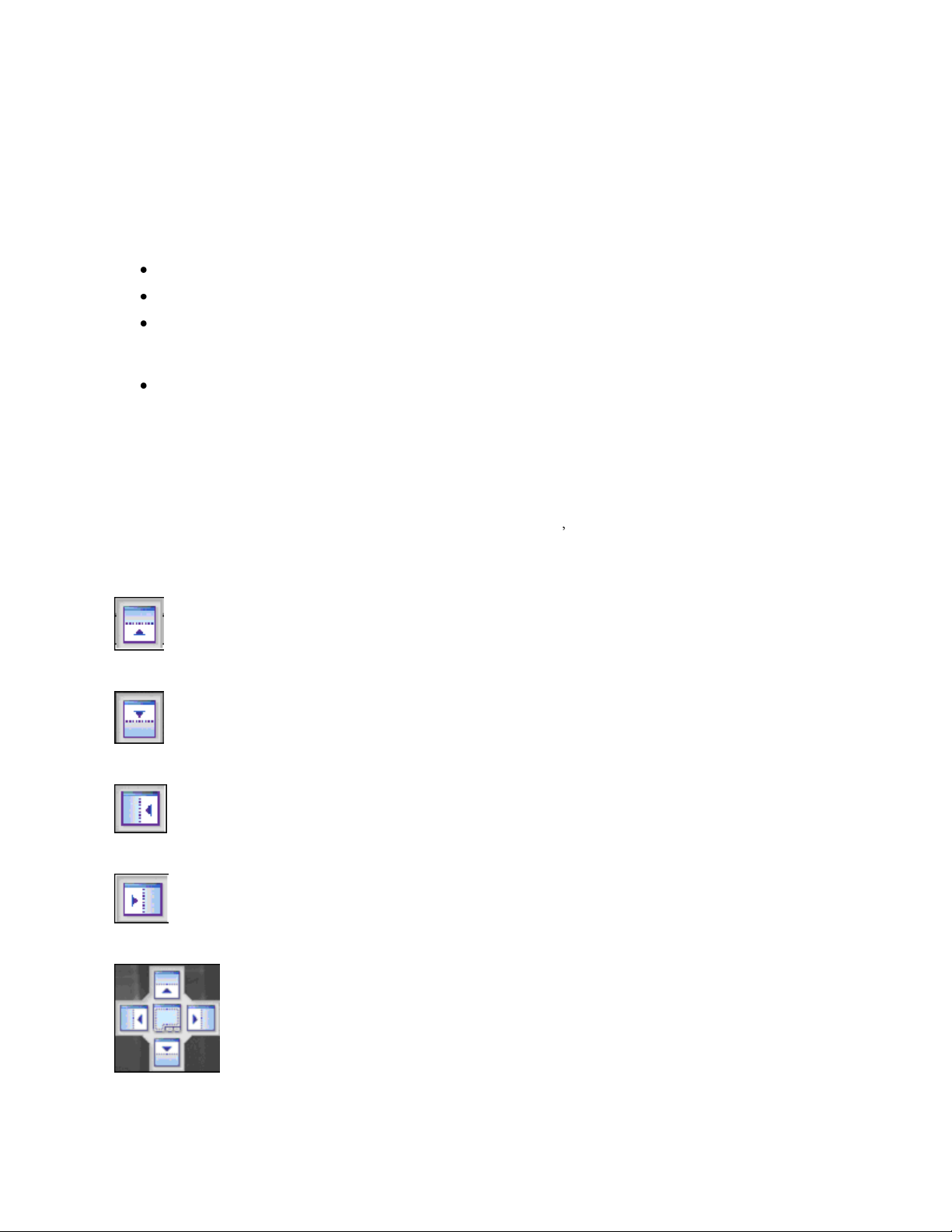
To move a floating plug-in module, click on the title bar of the module and drag it to any of the plug-in module position icons of choice. The following are descriptions of the plug-in module position icons.

Position the plug-in module at the top of the workspace

Position the plug-in module at the bottom of the workspace

Position the plug-in module at the left of the workspace

Position the plug-in module at the right of the workspace

Using Plug-In Modules

The center arrows console allows positioning of the plug-in module at the top, bottom, left or right of an empty workspace by using the exterior arrows

The center arrows console middle button allows positioning the plug-in module at the inside of another plug-in module

Histogram Controls

The Histogram Controls plug-in offers options for viewing tonal and color information about an image. By default, the histogram displays the tonal range of the entire image.

Go to View > Plugins to load the Histogram Controls plug-in.

Apply a Histogram

If the Histogram plug-in is not showing, choose Plugins > Histogram plug-in. From the stretch mode drop-down list, select None, Automatic or Manual. The Options button offers the choice to select the Y-axis, reset zoom or copy graph.

Digital Video Player

Purpose of the Digital Video Player Using the Player Player Features Player Options Extract or Delete Individual Image Files (Frames) Create a Sequence (.sqv) File by Merging Images Saving .AVI Files

Purpose of the Digital Video Player

Digital Video Player (DVP) in LS software clubs multiple images in a single file and shifts through the images, allowing users to select one (or more) of the clubbed images to analyze later.

Using Plug-In Modules

Use the SQV whenever possible. AVI file types reduce the image to 8-bit.

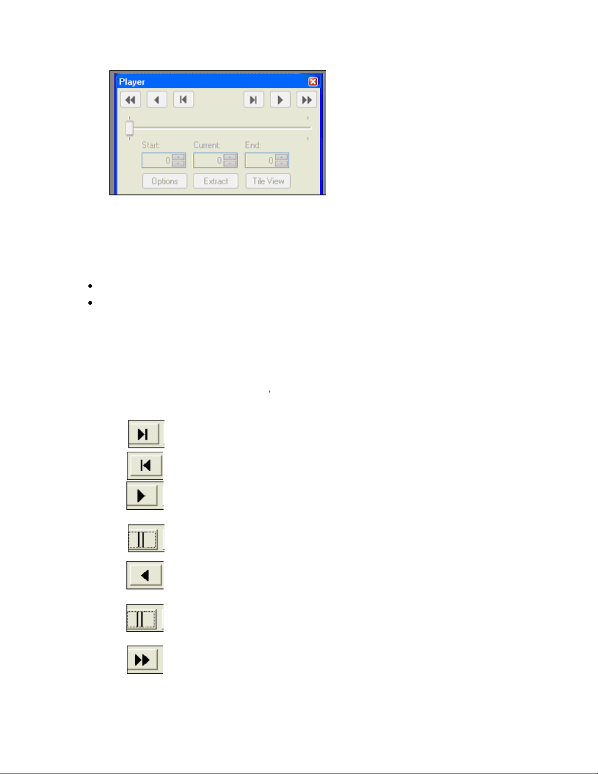
BUTTON

FUNCTIONALITY

Views the next image.

Views the previous image.

Plays the sequence of images. Playing will show the images one after another.

This button changes to a Pause/Stop button, which stops any kind of playing.

Plays the sequence of images in the reverse order.

This button changes to a Pause/Stop button, which stops any kind of playing.

Plays the sequence with a number of images to skip. The number of images to skip can be set in the Options dialog.

If a sample is to be observed over a period of time it is required to snap multiple pictures at regular and definite time intervals, maybe with progressively higher integration times.

Using the Player

To access the DVP function:

Go to View > Plugins and click on the Digital Video Player plug-in. The DVP comes up automatically, as soon as the image-capture process for Sequential and

Dynamic Integration is complete.

Player Features

Below is the description for each of the Player s buttons:

Using Plug-In Modules

Plays the sequence with a number of images to skip in reverse order. The number of images to skip can be set in the Options

dialog.

The Options button displays the Options dialog window to set Player properties.

This option lets the user work with individual frames (images) from a single .sqv file. Extract a single frame if required. A detailed description follows in this chapter.

Displays thumbnails of images in a tiled fashion. This can be useful in extracting specific images. When the player is active, this option also shows active scrolling and the currently active frame is highlighted red.

Frame Rate

This is the interval (in milliseconds) between two consecutive images that are displayed. For example, a value of 500 means that a new image will be displayed a half second after the previous image.

Frames per minute is automatically calculated based on this

value.

Frames per minute

This is the number of images that will play during a period of one minute.

Fast Frame Skip

This is the number of images to be skipped when playing with {bmc Doci0075.BMP} or {bmc Doci0076.BMP} button.

Repeat

When the Player reaches the end of the sequence of images, it starts again with the first image.

Play to end

When this option is selected, the player will stop when it reaches the end of the sequence of images.

Auto reverse

When this option is selected, the player goes back in reverse order after it reaches the end of the sequence of images.

Player Options

Click the Options button in the player to set individual options for going through frames in a .sqv or .avi file. Once Options is selected the following window appears:

Extract or Delete individual Image files (frames)

Extracting an image from a .sqv or .avi file creates new images in the workspace and DOES NOT remove them from the sequence. Deletion deletes the images them from the sequence.

The easiest way to initiate this action is by clicking on Tile View checkbox in the player, which brings up the following window. Just right click on any image to extract or delete.

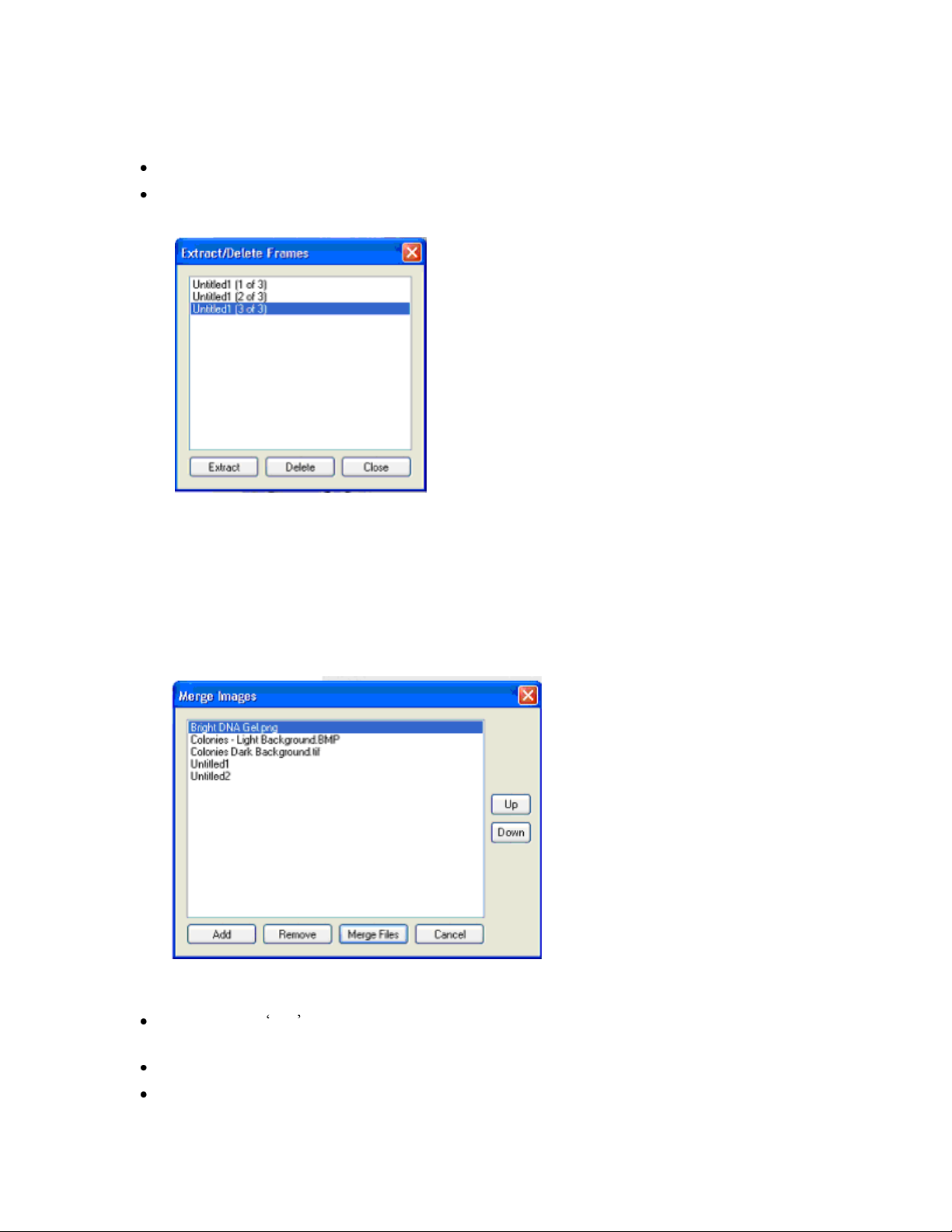
Using Plug-In Modules

The other two ways this action can be initiated is:

If the player is open, click on Extract from the player. If the player is not open, but the .sqv file is open, click on Images > Extract Frames.

The following window is brought up, that lists all the frames inside the .sqv in question:

All the images contained in the active sequence are in the list. The user can Extract (open the specified image in a new window) images or Delete (remove) images from the active sequence.

Create A Sequence (.sqv) file by Merging images

It is possible to merge existing files (or open images) and create a single .sqv file. This is a good way to keep all images in one single file. To create a sequence, select Image > Merge files. This feature can be used to merge images open in the LS workspace.

Controls:

Add: Click on Add button to find files from the hard-disk to merge. Existing files in the workspace

are automatically listed. Remove: Select a file and click on Remove to remove it from the list. Merge Files: Merges files in the list into a single .sqv.

Using Plug-In Modules

Note:

Use the SQV whenever possible. AVI file types reduce the image to 8-bit.

Cancel: Closes the window and cancels the process.

Saving .AVI Files

If files need to be shared with another researcher or opened in another place on another computer export the .sqv files to a standard universal format. (SQV is a custom format used by UVP LLC).

Audio Video Interleaved (AVI) is one such broadly acceptable format. (It is a simplistic Windows format that caters to the needs of slow animation, audio and video.)

To import an .AVI file, no special steps are required to be taken since it is one of the standard formats supported by LS Software.

To export a .SQV file to .AVI, use the Save As functionality provided by UVP Software. Depending on the requirement of the target player, AVI files may need to be compressed/ encoded using

a specific codec. Before exporting, LS software allows users to choose from one of the pre-installed codecs.

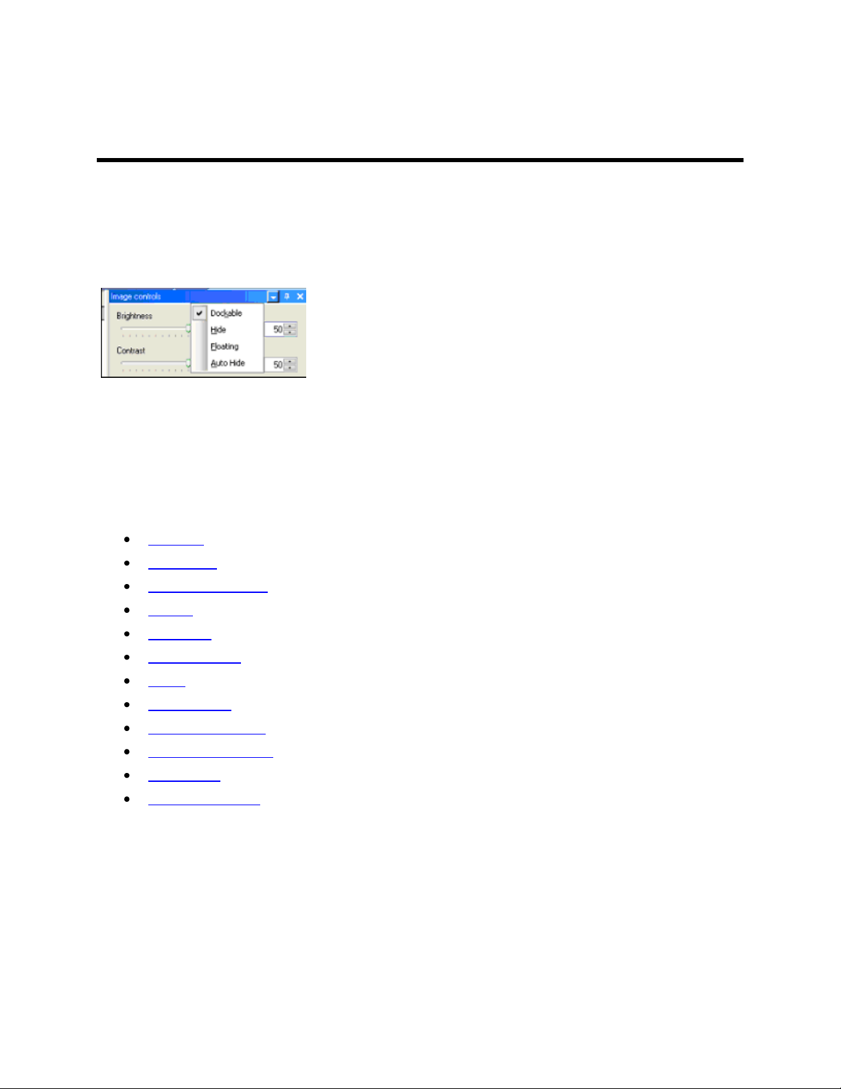
Image Controls Plug-In

The Image Control plug-in offers features to control how an image looks. Changes made to images using this plug-in will not be permanent changes to the image. All the changes can be reversed with the Reset button.

Go to View > Plugins to load the Image Controls plug-in. Specific features available on the Image Control module are:

Brightness: affects the overall brightness or dimness of the image. Brightness level of 50 means

the image is displayed in its original brightness (i.e. unchanged). Changing the brightness level

can make features near the top or the bottom of the intensity scale easier to see. Contrast: affects the difference between light and dark parts of the image. A contrast level of 50

means that the image is displayed in its original contrast. A level higher than 50 means that

contrast has been increased (lights are lighter, darks are darker). A level lower than 50 means

that contrast has been decreased (lights and darks are both closer to middle values). Increasing

the contrast tends to highlight differences in intensity level; decreasing it can make patterns that

cross intensities more clear. Gamma: also affects the difference between light and dark parts of the image, but it does so by

using a "gamma correction curve." The gamma correction curve affects middle values more

quickly than values at either the darkest or the lightest ends of the spectrum. Gamma contrast

values range from 0.1 to 5.0. A value of 1.0 means that no gamma correction curve is in effect

(the image is displayed at its original levels). Gamma contrast changes have similar results to

regular contrast changes. Invert: reverses all intensities, light for dark and dark for light. This also will have the effect of

complementing colors (e.g. red to turquoise, yellow to blue). Inverting the image can make certain

features easier to see.

Change Brightness, Contrast, Gamma Or Invert

Change Brightness

Using Plug-In Modules

Slide the Brightness control either left or right, or type a desired brightness value into the

Brightness text box to the right of the slider.

Image Before Effects Applied

Brightness Applied

Change Contrast

Slide the Contrast control either left or right, or type a desired contrast value into the Contrast text

box to the right of the slider.

Contrast Enhanced

Change Gamma

Slide the Gamma control either left or right, or type a desired Gamma value into the Gamma text

box to the right of the slider.

Using Plug-In Modules

Invert Image

Select the Invert check box. To stop inverting the image: clear the Invert check box

Inverted Image

Return to Default Values

After changing any of the Image Control options, click Reset to return all settings to the default settings.

3D Plots

The 3D Plots plug-in allows the user to see a three dimensional view of the sample. For example, if two bands look equally bright in an image, or with naked eye, a 3D plot can actually show if there is a quantitative difference in intensity.

A 3D plot can also be used as a great presentation tool. The uniformity of the light source in conjunction with the camera response can be checked using 3D

plots.

Using the 3D Plot Function

LS software 3D plots can be used for static images as well as live preview and integration.

Load an image into LS workspace. (It could be an image captured from the camera or an image

loaded from the disk.) Click on View > Plugins > 3D Plot Plug-in. This will bring up a separate window that shows the

3D plot.

Controls on the 3D plot window

Viewpoint tab

Controls on this tab let the user set the correct angle of view.

Rotation Controls:

One can rotate the image in Y as well as Z axes, using the Y rotation and Z rotation handles. The axes are as follows:

Z axis: The vertical axis.

Using Plug-In Modules

Y axis: The horizontal axis. X axis: The axis coming out of the plot, towards you.

The plot can also be rotated by dragging it with the mouse in desired direction.

Zoom Controls:

Zooming in and out of the plot is possible in two ways:

Using the buttons labeled Zoom In and Zoom Out Using the spin-box and adjusting the percentage.

Output tab

Three controls in this tab let you export the 3D plot information for various uses:

New Image: Pressing this button creates a new image in the LS workspace with what is visible

on the surface plot. This new image must be saved. Clipboard: Pressing this button copies the 3D plot onto clipboard, so that it can be pasted to any

other software (eg. MSWord, Excel, Paint, Photoshop etc.) Printer: Pressing this button prints the 3D plot on a desired printer. Pressing it brings up the list of

available printers.

FTP Transfer

The FTP Transfer plug-in allows the user to transfer files from one computer to another.

Click on View > Plugins > Ftp Transfer. This will bring up a separate window that shows the Ftp

Transfer plug-in. Enter the IP address of the system acquiring the image and the TS login and password in the

FTP plug-in preferences window. Start the software and take pictures. Press Connect button on the FTP plug-in after starting the software.

Log Viewer

The Log Viewer displays a log of user actions and presents the action list to the user in a log box.

Go to View > Plugins to load the Log Viewer plug-in.

Zoom/Pan

The Zoom/Pan plug-in allows the user to magnify a part of the image. Once the user zooms in on the image, the entire image will no longer be visible in the window. The user may easily change the portion of the image that is visible by panning.

Using Plug-In Modules

Go to View > Plugins to load the Zoom/Pan plug-in.

Using Zoom In or Out

Click on Zoom In or Zoom Out (located below the thumbnail version of the image on the Effects

tab, on either side of the slider).

Slide the zoom slider to the left to zoom out or to the right to zoom in.

Select the desired zoom factor from the drop-down list to the right of the slider and buttons.

TIPS: There is no need to "turn off" the Magnify tool -- it will be turned off automatically by selecting any other tool (such as a selection tool or an annotation tool).

The image can also be magnified selecting View > Zoom and clicking on the desired zoom percentage. In the drop-down box, enter a number and press TAB. (The drop down box is particularly useful if a zoom

factor is needed between the pre-defined choices in the list.)

Pan to a Different Part of the Image

In the thumbnail image, drag the Pan rectangle to the desired location. If the desired location is outside the Pan rectangle, simply click the desired location to "jump" the

pan rectangle there.

Magnify Part of an Image

Click the Magnifying Glass button. The mouse becomes a magnifying glass. Click anywhere on the image to magnify an area. Adjust

the Magnify factor number to increase or decrease the magnification. To show annotations under the magnifying glass, click the Magnifying Annotations option.

Camera Plug-In

The camera capture plugin provides camera controls for all Canon digital color cameras. To open the capture tab, go to View > Plugins > Camera Plug-in. The module offers the following

settings and controls in automatic mode (turning the dial of the camera to A-DEP).

Color Capture: Determines whether the camera captures in color or monochrome. Brightness: Adjusts the brightness of the image. Start Preview: Preview a live image. Capture: To capture an image. Reset Camera Connection: Reestablish the connection of the camera to the software.

In Manual mode (turning the dial on the camera to M) users may adjust the following parameters:

Camera Plug-In

Template: This button allows users to define templates to save customized setting and displayed

features. Set-Up Canon Capture Templates Aperture: The degree to which the shutter will open. Shutter: The speed at which the shutter will be snapped. Quality: Consists of Image Resolution and Compression – extra fine, fine, normal. Select extra

fine for the least compression and highest quality. Resolution: Select from the drop down menu. White Balance: Select from the drop down menu.

The following image is the Previewed image. The focus can be automatically or manually adjusted.

Camera Plug-In

Capturing Images

This topic discusses the process of capturing images using LS software. The following sections explain the process in more detail:

To capture an image with the camera:

If the camera plug-in is not showing in the software interface, select View > Plugins and load the

camera plug-in for the camera.

Place the gel (object to be captured) into the darkroom Turn the camera to A-DEP. Select Preview in the camera plug-in. If the settings are not correct, change the camera dial to M to manually control the settings of the

camera. When the optimal settings have been found, click onto Capture. .

Creating Templates

Set-Up Templates

Templates enable users to configure specific settings along with unique designator name to camera and darkroom/lens plug-ins. Templates allow users to then select the defined settings as needed.

Set-Up a Canon Capture Template Set-Up a Colony Template

Edit and Delete Templates

Edit a Template

While in the Plugin click on the Templates drop down menu. Select the template to edit from the drop-down list. The default values and will be set to the

values used for that template. To edit the name, click Edit Name to the right of the window. Type a new name and then click

OK. To change the template settings, click Sync. This allows experimentation with changes to

settings and then allows those settings to be saved. To change any setting default, select the new value for that setting. Click Save (or OK) to save the changes.

Delete a Template

While in the Plugin click on the Templates drop down menu. Select the template to be deleted from the drop-down list. Click Delete. Confirm the deletion of this template by clicking Yes.

Tip: Make many template changes at once by using Save instead of OK.

Set-Up Canon Capture Templates

Capture Templates are groups of preset camera settings. They are used on the Canon Camera Plug-in either to return the camera quickly to a group of settings used often or to default some settings while making others available for alteration.

Each template has a name, a default value for every camera setting and a list of flags indicating which settings will be excluded and which will be shown from the Canon Camera Plug-in when this template is

Creating Templates

Tip:

To copy a template, select the template to copy first, then click New. The new template will use the one selected for initial values.

To save a template in Step 1 of 2: Select Classes, add the desired points and

classes if not already selected) and click the New button in the Template section of the window.

A new pop-up window will ask for a new Template name. Type in the new name and select OK. The Template name window will close and direct back to the Step 1 of 2: Select

classes tab.

selected. If a setting (or group of settings) is not excluded, it can be overridden on the Canon Camera plug-in before each capture.

Create a New Template

On the Canon Camera Plug-in click on the three dots next to the drop-down Templates menu.

The Capture Templates window will appear. Click New. The New Template window will appear. Type a name for the new template and click OK. A new template will be created and then

defaulted to the current settings in the Capture Templates window. Set each camera setting to the desired value. On the right hand side, there is a list of features that can be included in the controls. Check the

features (controls) to use in the template. Only those checked will appear in the main capture-

panel. Click Save (or OK) to save the new template.

Creating Colony Templates

Templates allow the user to set parameters for colonies most frequently counted and provides a quick count of Petri dishes commonly used by the lab.

Click on the Count button to proceed to the Step 2 of 2: Finish tab.

If the shape and size sliders are changed to capture additional colonies, click Save

filters in the Templates section of the window to save the new settings.

Select Finish to complete the count and save the template.

A new pop-up window will ask for a new Template name. Type in the new name and select OK. The Template name window will close and direct back to the Step 2 of 2: Finish

tab.

Click the Finish button to complete the count process and save the template.

Related Topics:

Manual Counting User Defined Template Counting Zone Counting Spiral Counting Renumbering Colony/Zone Values

Creating Templates

Deleting Colony Counting Templates

To delete a Template, from the Colony Count module:

Click Start Colony Count. Click Manual Count. Click OK. Click on the Step 2 tab. Under the Template section, click the drop down menu. Select the Template name to delete. Click Delete.

Editing Images

Note:

The Edit menu also offers a Cut feature that can be used while editing text in LS Software. Cut does not work on images.

If there is a ROI present on the iamge, click away from the ROI once to cancel it.

Choose Copy from the Edit menu.

Select a ROI on the image using one of the selection tools.

Choose Copy from the Edit menu.

Note:

Copy can also be used on text, in which case it acts in the standard Windows fashion. Copied images or sections of images will include annotations if the annotations were

displayed when Copy was used. If annotations were hidden, they will not be included.

Tip:

Copy also is available by using the Ctrl-C accelerator key, by using the Copy button on the Toolbar and by using the shortcut menu on the Image window itself.

Editing Images

Overview

Undo and Redo Copy Paste and Paste Special

Using Selection Tools (Region of Interest Tools)

Overview

The image editing features provided in LS Software allow users to undo changes to images, to copy images or parts of images, to paste images from the clipboard as new images and to merge clipboard images with existing images.

Most editing features are found on the Edit menu. However, to be able to use all editing features, you will also need to use the Selection Rectangle and Selection Ellipse tools from the Tools menu.

Copy

Used on an image, the Copy command copies all or part of the image to the clipboard.

Copying an Entire Image

Copying a Selected Region Within an Image

Editing Images

Note:

Paste can also be used on text, in which case it acts in the standard Windows fashion.

Paste

This command takes an image from the clipboard and imports it into the software, displaying it in a new Image window.

Paste an Image

From the Edit menu choose Paste. The image will be displayed in a new Image window.

Note: Paste is only available if there is an image on the clipboard.

Paste Special

This command allows an image on the clipboard to be merged into the current image. It is useful for adding comparison or reference information into an image, for making composite images and for testing two images against one another for motion.

To modify the Paste Special options, go to Edit > Paste Special Options:

The following merge modes are available in all the Software:

Blend: mixes the incoming image with the current image in a selected proportion. If the Source

proportion (Src%) is set to 100%, pixels in the incoming image replace those in the existing image

without mixing (i.e. the incoming image is copied entirely over the existing image wherever it

lands). Blend is used primarily to place comparison information into an existing image, especially

when using high proportions. Add: adds pixels in the incoming image to those in the existing image up to maximum intensity.

Add is used primarily to build composite images with little or no overlap. This feature requires no

additional settings. Subtract: subtracts pixels in the incoming image from those in the existing image. Subtract is

used primarily to test for differences in or motion between two otherwise similar images. This

feature requires no additional settings.

Undo and Redo

The Undo command will undo the last material change made to an image. Material changes include all manipulations and the Paste Special command. The Redo command reverses the last Undo. To see what the last material change did in detail, alternate between Undo and Redo. Changes made through the plugins do not permanently change the image.

Undo the Last Change to an Image

With the image open from the Edit menu, click Undo. The former version of the image will be restored.

Redo the Last Change to an Image

With the image open from the Edit menu, click Redo. The last change will reappear. The Redo command will be unavailable until Undo is used for the first time.

Editing Images

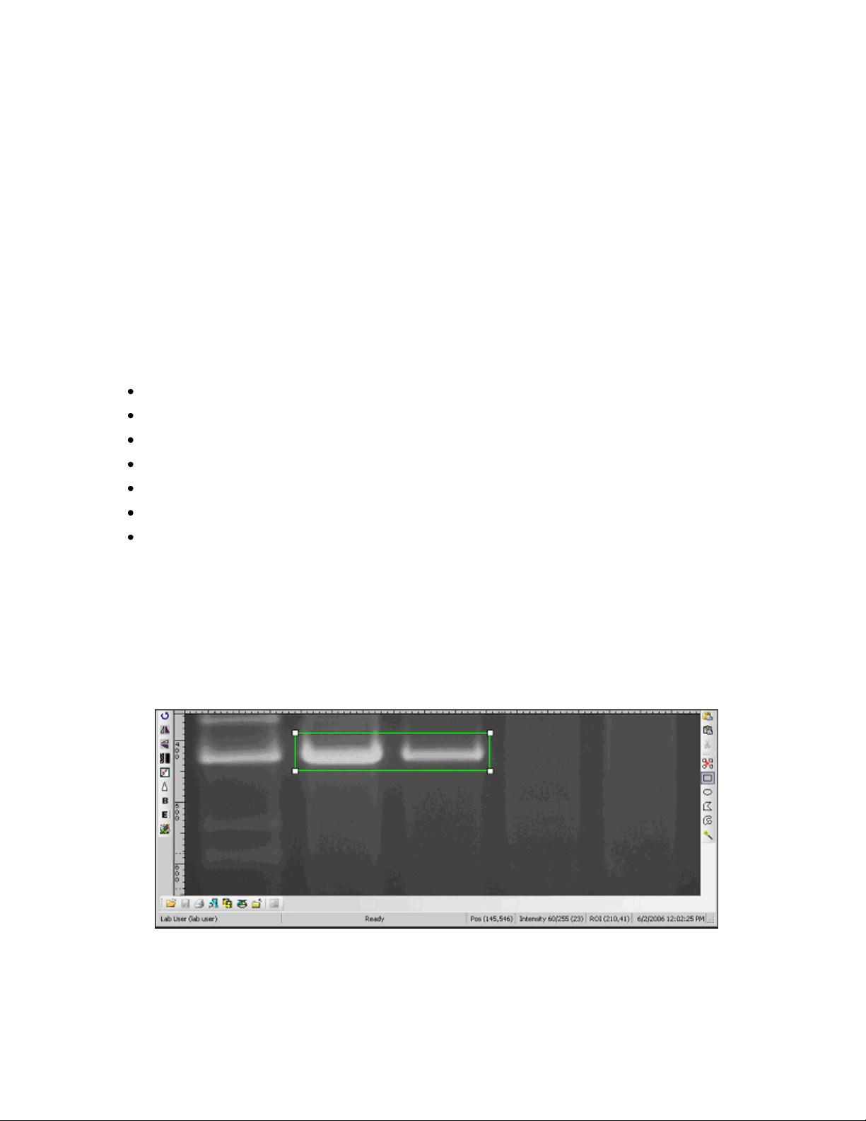
Using the Region of Interest Tools

Using the Selection Tools

These tools allow users to mark part of the image for use in other operations. LS software provides several Region of Interest (ROI) selection tools:

ROI tools (left to right): New ROI, Rectangular ROI, Elliptical ROI, Polygonal ROI, FreeForm ROI and Magic Wand ROI. Select the tools from the toolbar or from Tools > Region of Interest (ROI).

Rectangular, Elliptical, Polygonal ROI: To define a rectangular, elliptical or polygonal type of

ROI, start with the upper-left corner of the desired region and drag the mouse downward and to

the right until the desired area is marked. FreeForm ROI: To define a ROI with the mouse pointer, keep the left mouse button pressed and

draw around the region of interest. Lift the mouse button to automatically complete and enclose

the area. Magic Wand ROI: To mark the ROI automatically on the image, click just once inside the region

of interest and the software marks that area by identifying the edges. Zoom in on the image to get

a better outline of the ROI. The spin-box Range is the sensitivity of finding the edges, and is

dependent on the dynamic range of the image. Lower the number, smaller is the area.

Apart from Analysis features, two operations in the software use an area of interest: Copy and

Crop. Copy will copy the selected region to the clipboard. If there is no selected region, the entire

image will be copied. Crop will remove (crop away) all parts of the image outside of the selected

region. Either operation will work with either selection tool.

Select a Region

Choose the desired selection tool either from the Tools > Region of Interest (ROI) or from the

toolbar. Starting with the upper-left corner of the desired region, drag the mouse downward and to the

right until the desired area is marked.

Adjust the Region

If the selection is not quite right, move it or resize it without having to start over:

To make the selection wider or narrower: drag the left or right dotted lines that bind the selection

to the desired size. To change both height and width at one time: drag any corner control point to the desired size. To move the selection: click on and drag the interior of the selection to the new location.

Cancel the Region

Click once anywhere on the image away from the current selection. The selection markers will

disappear.

Using Image Filters

Overview

Filter Navigation Image Filter

Background Correction and Subtraction

Tip:

A record of image filters applied to an image is kept in the image's Image History.

Tip:

See information on Undo in the Editing Images section. For additional information on Saving images, see Loading and Saving.

Using Image Filters

Overview

LS Software offers several types image filters. Each filter makes a substantial and material change to the image itself. In general, the results of an applied filter are not reversible. Image filters can be used to correct for problems in preparing for and in acquiring the image. They also can be used to expose new information in an image by removing or de-emphasizing other information. Any changes to the image are logged in the image history data, which also offers a notes sections.

To get the most from image filters, it is important to understand the following features first:

Undo: Undo reverses the last filter performed on an image. Saving: Saving stores an image on disk. Saving as another file name allows users to return to a

former version of an image.

Filter Navigation

The software provides three different ways to access the Image Filter tools:

From the toolbar menu Image > Filters drop-down menu View > Plugins > Filters plug-in

Filter Menu

The Image > Filters menu, allows users to perform the same commands as in the Filter Plugin. The Filters plug-in offers several types of image filters to make changes to an image. Filters can be used to adjust the resulting image. In addition to accessing the filters from the plug-in module, select filters from the Image > Filters menu.

Filter Plugins

The Filter plug-in will display with the following functions. Go to View > Plugins to load the Filters plug-in.

Using Image Filters

Geometry Filters

Rotate: Rotates the image around its center, useful for aligning images taken with a crooked gel. Align: Aligns the image to an adjustable grid. Flip Horizontally: Mirrors the image right for left, correcting for an upside-down gel. Flip Vertically: Mirrors the image top for bottom, also correcting for upside-down gels in the other

direction. Resize: Enlarges or reduces the image in size, uses less space and memory, and enables the

image to be seen on the entire screen.

Color Filters

Reduce to Mono: Removes color from the image, making it monochrome. Convert: Allows user to change the bit depth of the image

Image Enhancement Filters

Remove Noise: Removes periodic (patterned) noise in the image Despeckle: Removes single-pixel flaws in the image (called artifacts) Sharpen: Sharpens edges in the image, making them more pronounced Blur: Dulls edges in the image, making them less visible Emboss: Gives the image a "chiseled in stone" look Starfield subtraction: Removes the star-like single shot noisy spots in dark images taken with long

exposures

Duplicate Image: Creates a copy of the image

Burn Changes onto a New Image: Creates a copy of the original image and makes all the

changes made to the image permanent.

Background Filter

Background Correction

This command allows users to subtract a flat level of intensity off the current image.

Background Subtraction

This command allows users to subtract one image from another.

Using Image Filters

Note:

If the image to be duplicated has been previously saved, the new copy will not inherit the old copy's filename. Instead, the new copy will be an unsaved image.

Burn Changes to a New Image

The Burn Changes to a New Image command takes all the changes made to the image and creates a duplicate copy in a new file. This process is called "burn" because once the changes are made, they are not reversible. Burning changes to a new image is useful when creating a document or presentation.

Click onto Burn changes to a new image from the Filters plug-in or use the Image > Filters > Burn

changes to a new image command. A second copy of the image will appear in a new image window as an untitled image.

Convert Image

The Convert filter converts an image bit and color depth when needed.

Click onto Convert from the Filters plug-in or use the Image > Filters > Convert command.

Reducing a large image to monochrome may take a few seconds. Select new depth and click

OK.

Duplicating Images

The Duplicating Image command creates an identical copy of the foremost image. The new copy will appear in its own Image window.

Click onto Duplicate image from the Filters plug-in or use the Image > Filters > Duplicate image

command. A second copy of the image will appear in a new image window as an untitled image.

Flip Image

Flip Horizontally

This filter provides a right to left mirror-image. Two clicks of the flip button will return the image to its starting orientation.

Click onto Flip horizontally from the Filters plugin or use the Image > Filters > Flip horizontally command.

Using Image Filters

Flip Vertically

This image filter mirror-images an image, top for bottom. Unlike most image filters, it does not degrade the image and may be used repeatedly with no ill effect. Two uses of the filter will return the image to its starting orientation.

Click onto Flip vertically from the Filters plug-in or use the Image > Filters > Flip vertically command.

Image Enhancement Filters

Image enhancement tools allow users to highlight important features and remove unwanted signal in the image.

Remove Noise Despeckle Sharpen Blur Emboss Starfield Subtraction

Remove Noise

This filter removes periodic (patterned) noise from an image. Patterned noise is removed by creating a frequency-space mapping (Fourier transform) of an image and removing frequency spikes away from the graph's origin.

There are two issues to be aware of with noise removal. First, if the image has actual (desired) pattern information, the operation will not be able tell these from noise and it will remove them. Second, the mathematics of the operation can cause some edges pixels to be identified as patterns, resulting in blurring on some images.

Click onto Remove noise from the Filters plug-in or use the Image > Filters > Remove noise

command. Removing noise a large image may take ten or fifteen seconds.

Despeckle

This filter removes single-pixel flaws (called artifacts) from an image. For many reasons, the image capturing process and hardware might misread isolated individual pixels as either white or black. The Despeckle filter mathematically identifies and removes these "loner" pixels.

There are two issues to be aware of with the Despeckle filter. First, if the image has actual (desired) single-pixel bright or dark areas, the operation will not be able tell these from artifacts and it will remove them. Second, the mathematics of the operation can cause some edge pixels to be identified as "speckles," resulting in slight blurring on some images.

Click onto Despeckle from the Filters plug-in or use the Image > Filters > Despeckle

command. Despeckling a large image may take a few seconds.

Sharpen

This filter enhances edges in an image, making them more visible. It is easier to see fine detail after an image has been sharpened.

Using Image Filters

Tip:

Use the arrow keys to cycle through all eight directions while watching the Preview.

Click onto Sharpen from the Filters plug-in or use the Image > Filters > Sharpen command.

Sharpening a large image may take a few seconds.

Blur

This filter blurs edges in an image, making them less prominent. You can see gross (large-scale) detail more easily after the edges have been blurred because details that may have been obscuring it are removed.

Click onto Blur from the Filters plug-in or use the Image > Filters > Blur command. Blurring a

large image may take a few seconds.

Emboss

This filter gives an image a "chiseled in stone" look. Edges take on a three-dimensional (3D) appearance, making them stand out vividly.

Emboss can be performed from any of eight cardinal directions. Conventionally, these are referred to as North (up), Northeast, East (right), Southeast, South (down), Southwest, West (left) and Northwest.

The easiest way to think of the "direction" of the embossment is as the location of a strong light source around the image. For example, if North is selected, the image will appear as if it is illuminated with a strong light from the top. Therefore, horizontal edges will be strongly lighted on the top edge and shadowed on the bottom, and vertical edges will tend to disappear. Diagonal edges will be shadowed in direct proportion to how closely they are horizontal. Alternatively, if East is selected, vertical lines will be shadowed on the left side and lighted on the right side. Horizontal lines would become harder to distinguish.

Click onto Emboss from the Filters plug-in or use the Image > Filters > Emboss command.

The Emboss window will appear. Select the desired Emboss Direction. The Preview window will show a thumbnail sample of

what the image would look like embossed from this direction.

Click OK.

Starfield Subtraction

This filter eliminates starfield shaped pixel flaws from an image. When long exposures are necessary to capture an image, bright pixels in the shape of a star may appear in the image.

To subtract the starfield:

Choose Filters > Starfield Subtraction.

Image History

Each material change to an image is tracked in the software s Image History feature. Material changes include use of any filters applied and use of the Paste Special feature. Changes to Effects and

Annotations are not tracked in the Image History.

Using Image Filters

Choose Tools > Spatial Calibration > Measure Length

Click one edge of the feature.

Move to the other edge of the feature. As the mouse is moved, the scale tool will show

how many pixels (unless the calibration process has been performed) are contained in the straight line drawn with the tool.

Click the other edge of the feature. The image will now display the total length

Viewing Image History

Each material change to an image is tracked in LS software s Image History feature. Material changes include use of any filters applied and use of the Paste Special feature. Changes to Effects and

Annotations are not tracked in the Image History. Entries in the Image History may be of three types:

Creation: Describes how an image was created (captured or scanned) and provides some

details. Change: Describes use of image filters or Paste Special. Error: Describes an error that occurred while reloading the image from a saved file. The main use

of an Error entry is to track the times when the image was changed in another software package,

which is important for some kinds of laboratory practice.

The Image History includes information on:

What type of entry it is, from among the types described above. When the change occurred. What the change was and details about it. Any notes that you add to explain the entry.

Adding Notes in the Image History

Right click on the image, choose Image Information. The Image Information window will be

displayed. Click the History tab at the top of the window. Click on any history entry in the list on the left side to display details about the entry. To Add Notes to a History Entry. Display image History as described above. Click on the history entry to which to add notes. Type the notes in the Notes field. Repeat steps for any other history entries. Click OK.

Note: Image History is useful in Supporting 21 CFR Part 11 Compliance

Measurement Tools

Measure Length

Using Image Filters

measurement value.

Right click on the new measurement annotation displayed to change the appearance of

the annotation. If desired, change the line thickness, line style, font size, or general formatting of the line and value displayed.

Choose Tools > Spatial Calibration > Measure Angle

Form a line by clicking on one edge of the feature and then click again to finish the line.

To measure the distance between the line just drawn and second line, move the mouse

away from the line. Notice how as the mouse is moved, the scale tool shows how many degrees are contained in the angle drawn with the tool.

Click to freeze the angle in the desired position. The new angle measurement

annotation now appears.

Right click on the new measurement annotation displayed to change the appearance of

the annotation. If desired, change the line thickness, line style, font size, or general formatting of the line and value displayed.

Choose Tools > Spatial Calibration > Measure Area

Form a rectangle by clicking onto the image and drawing the rectangle on the image.

Click again to finish changing the shape of the rectangle.

The new area measurement annotation now appears in pixels (unless the calibration

process has been performed).

Right click on the new measurement annotation displayed to change the appearance of

the annotation. If desired, change the line thickness, line style, font size, or general formatting of the line and value displayed.

Place one of the images on the clipboard using the Copy command. If desired, a sub-

region of the image can be used.

From the Edit menu, choose Paste Special. The Paste Special window will appear.

Measure Angle

The measure angle tool requires three points to be placed on the image to define an angle.

Measure Area

NOTE: Length Measure and Area Measure annotations use the image's scale in calculations. If

these annotations display information in pixels ("px"), no scale has been set. See "Changing

Sample Width" for instructions on setting the image's scale.

Merging Two Images

Merging results in a new image that includes the existing image plus all of the area of the incoming image, even if that area is off of the edge of the existing image. This allows the composition of "mosaic" images (usually with Add) by placing the incoming image at the edge of the existing image.

Using Image Filters

Tip:

Paste Special also is available from the Toolbar and the Image window's shortcut menu.

If the incoming image is large, select the Preview Frame Only check box to allow

repositioning of the incoming image without the lag caused by redrawing a large image. Otherwise, clear the check box to preview the result.

Select the desired merge operation: Blend, Add or Subtract.

If using Blend, set the desired blend percentage.

Click OK.

Moving the mouse over the existing image, position the merge as desired. The merge

results (or positioning frame, for Preview Frame Only) will be previewed as the mouse is moved. Position the upper-left corner of the incoming image. Once positioned, the selection can be moved.

When the desired position is reached, click the right mouse button once. Merges that

involve large images may take a few seconds to complete.

Obtaining Image Information

Overview

LS Software keeps various sorts of information about an image. This Image Information includes:

Image Scale: Described as the number of metric units in the image's width, this information is

used to calibrate Rulers and Measurement Annotations. Image Scale is also described under

Spatial Calibration.

Image Resolution: The width and height of the image in pixels. Image Depth: The number of bits used to represent intensity. LS Software supports 8-bit, 12-bit

and 16-bit image depth. Notes: Enter notes about an image. File Properties: The file name, path, create date and size. All will be "N/A" if the image has not

yet been saved. Image History: A list of material changes to the image, when they occurred and any notes to add

about why or how the change was made are shown in the Image History.

To be more compact, the Image Information window is organized into two tabs. All information

except Image History is on the first tab; Image History is on the second tab.

To Display Image Information

If the image is not the foremost image, select it from the Windows menu or click its title bar. Right click onto Image Information. The Image Information window will appear. To switch between Image History and Properties, click the appropriate tab at the top of the

window.

Using Image Filters

Note:

An uncalibrated image will have "Pixels" as the unit type. If the unit type is Pixels, the number of units is the number of pixels in the image width and cannot be changed.

To Enter Notes

Display the Image Information window as described above. In the Properties tab, type information into the Notes text box. Click OK.

Calibrating Image Scale

Each image in LS software can have a scale associated with it. Scaling information is used to display rulers, measure length and measure area annotations. Refer to Spatial Calibration for information on using this tool.

Images scanned into the system from a scanner or imported from another program are not calibrated. In these two cases, therefore, you may wish to adjust or to set the image's scale.

Pseudocolor

The Pseudocolor applies a false-color spectrum to a monochrome or colored image. This process is sometimes called "colorizing." There are two primary reasons for using pseudocolor:

To make the image look more like what might be seen under a microscope with various kinds of

lighting, primarily for comparison purposes. To highlight specific intensities for analysis purposes. For example, one of the pseudocolor

spectrums highlights black (intensity 0) pixels with blue and white (maximum intensity) pixels with

red. This identifies the undersaturated and oversaturated parts of the image.

Go to View > Plugins to load the Pseudocolor plug-in.

Pseudocolor Spectrums

LS software supplies built-in pseudocolor spectrums:

Over-Undersaturation: Colors pixels in top 5% of dynamic range red and next 5% as yellow. For

example, in a 12-bit image, pixels with intensities 4095 to 3891 (5% range) will be colored red

and the next 5% range 3890 to 3685 will be colored yellow. There is no indication for

undersaturated pixels. Ethidium Bromide: Mimics the colors used in Ethidium Bromide gel preparation. Fluorescein: Mimics the colors used in the Fluorescein process. Green Fluorescent Protein: Mimics the green fluorescent protein colors. Texas Red: Mimics the colors that appear with a Texas Red stain. SYBR Gold: Mimics the colors that appear with a SYBR Gold stain. SYBR Green: Mimics the colors that appear with a SYBR Green stain.

Using Image Filters

SYPRO Orange: Mimics the colors that appear with a SYPRO Orange stain. SYPRO Red: Mimics the colors that appear with a SYPRO Red stain. Coomassie Blue: Mimics the colors that appear with a Coomassie Blue stain. Silver: Mimics the colors that appear with a Silver stain. Blue to Red: Colors all intensities from blue at the low end to red at the high end using a natural

light spectrum. Red to Blue: Colors all intensities from red at the low end to blue at the high end using a natural

light spectrum. Blue: Colors all intensities from black to bright blue. Cyan: Colors all intensities from black to bright cyan. Green: Colors all intensities from black to bright green. Magenta: Colors all intensities from black to bright magenta. Red: Colors all intensities from black to bright red. Yellow: Colors all intensities from black to bright yellow.

Apply or Remove a Pseudocolor

If the Pseudocolor plug-in is not showing, choose Plugins > Pseudocolor plug-in. From the Pseudocolor drop-down list, select the desired pseudocolor. The image will be colorized

as desired. To remove a Pseudocolor, from the Pseudocolor drop-down list, select None.

Reduce Image to Mono

The Reduce to Mono filter reduces a color image to monochrome. This is primarily useful when colors in an image are distracting rather than informative. For example, if light strikes certain surfaces from some angles, a "rainbow effect" (prism) will appear. Another use is to adapt for some software packages and techniques that require monochrome images or which are less reliable on color images.

The Reduce To Mono filter uses a weighted mix of colors to arrive at each pixel's monochrome intensity. Green is very heavily weighted while blue is almost disregarded.

Click onto Reduce to mono from the Filters plug-in or use the Image > Filters > Reduce to

mono command. Reducing a large image to monochrome may take a few seconds.

Resize Image

The Resize filter allows the image to be changed in size. It replicates or merges pixels as appropriate to arrive at the new size. Resize most commonly would be used to create a smaller version of a very large image to allow users to increase response time when applying filters or to import the image into another software package that does not accept large images.

Using Image Filters

Tip:

There is little point to increasing an image's size, although the filter does support it. Such an image would have more physical pixels after the operation, but it does not gain any new information content.

Note:

To distort the image, clear the Maintain Aspect Ratio check box and type the new width and height. This should be used only to reverse a similar distortion created in the image capture process.

Tip:

Rotations by 90, 180 or 270 degrees do not degrade the image. These operations can be completely reversed by a rotation of the same amount in the opposite direction.

Click onto Resize from the Filters plug-in or use the Image > Filters > Resize command. The

Resize window will appear. Select the desired new size from the drop-down list of suggested sizes.

Select the Enter Desired Dimensions option and type either the desired new width or the

desired new height.

Click OK. Resizing a large image may take a few seconds.

Rotate and Align Image

Rotate an image by an arbitrary number of degrees. Rotate is helpful to correct for a misaligned gel. Graphically select the degree to align the image based on an internal image feature.

Rotate an Image

Click onto Rotate from the Filters plug-in or use the Image > Filters > Rotate command. The

Rotate window will appear and a grid will be overlaid on the image.

Drag the grid so the yellow arrow moves in the direction you would like the image rotated. Once the grid is oriented to the desired position, click OK on the Rotate window.

Rotate an Image by an Exact Number of Degrees

Rotate the image by an exact number of degrees. For example, correct for an upside-down gel by

rotating it by 180 degrees. Click onto Rotate from the Filters plug-in or use the Image > Filters > Rotate command. The

Rotate window will appear and a grid will be overlaid on the image. For this operation, you will

ignore the grid. On the Rotate window, type the desired number of degrees into the Angle text box. Click OK.

Using Image Filters

Note:

The scale information used by the rulers also is used by measurement annotations. Length measure annotations can be used to see the length of a feature that is not square to the rulers.

Tip:

The device you select will remain the default until it is changed, even after rebooting. Generally, if you have only one TWAIN device, it will already be the default.

Align an Image

Align tool rotates the grid overlaid on the image so that it can be aligned with vertical/horizontal features of the image to make it easy for the user to select the # of degrees rotation.

Rulers

Rulers are located at the top and left of each Image window. The rulers show the width and height of the visible portion of the image either in metric units (if calibrated)

or in pixels (if un-calibrated). When zooming in and out of the image the, software updates the rulers to show the actual size and position of the visible portion of the image. As the user moves the mouse over the image, markers show the position on each ruler.

The units are shown in the upper-left corner (see the image above). Pixels (uncalibrated) are abbreviated "px;" all other values use standard abbreviations. When the rulers are calibrated to a standard measure, they may change units as zoom is applied to the image detail. For example, an image calibrated in centimeters may switch to millimeters when zoom is used. The measurements are still completely accurate; the rulers switch units because they are designed to show a useful number of units at every point.

Showing or Hiding the Rulers

Rulers may be hidden or shown individually for each Image window. Hiding the rulers provides

slightly more space in which to view the image. On the View menu, click View Rulers.

Scanning Images

LS software can acquire images from scanners that supply a TWAIN interface. (Almost all scanners support TWAIN.) TWAIN helps scanners provide their own software interface during scanning.

Select the Desired Scanner

Choose Image > Scan > Select Scanning Source. The Select Source window will appear. Select the desired device from the list. Click Select.

Using Image Filters

Tip:

Most scanners offer a "fast preview" mode. You can use this to adjust brightness, contrast and other settings appropriately before scanning.

Choose Tools > Spatial Calibration > Define Image Scale.

Find the feature in the image for which the size is known. Click one edge of the feature.

(It may be useful to position a small ruler with the Petri dish and capture the image of the ruler and Petri dish together so that the ruler can be used for reference)

Move to the other edge of the feature. As the mouse is moved, the scale tool will show

how many pixels are marked with the tool.

Click the other edge of the feature. The Set Scale window will appear.

In the Set Scale window, select the metric unit for the marked area (e.g. centimeters)

and enter the number of units (e.g. 12). NOTE: The marked area must be selected first and then the number of units second.

Click OK. The rulers will reflect the new scale.

Right click onto the image and select Image Information for the image.

There are two tabs present in the Image Information window. Ensure that the

Properties tab is selected.

In the Overall Sample Width area, select the unit measurement (the right-most drop-

Scan an Image from a Scanner

Select Image > Scan > Start Scanning. Change any settings offered by the device as desired. Consult Help for the scanner to learn

about the Scan dialog window for your device. Click Scan (this button may have different names, including OK or Acquire, for different devices).

The image will appear in a new Image window inside the workspace.

Spatial Calibration

Using the Image Scale Tool

There are two ways to set the image's scale:

If the size of a single feature anywhere in the image is known, use the Scale Tool to set the scale

of the entire image from that one feature. If the size of the entire image is known, change the Sample Width through the Image Information

window.

Calibrate the Image Using the Scale Tool

Changing the Sample Width for an Image

Sample Width is calculated from the width of the image. It is the distance of the width of the scene in the image. For reference, a ruler may be placed across the top of the image so that the entire distance of the scene can be determined.

Using Image Filters

down list) first. For example, if the sample width of the image is 500 cm, select centimeters.

Type the number of metric units in the text box immediately following Overall Sample

Width. For example, if the sample width of the image is 500 cm, type "500."

Click OK.

Note:

Length Measure and Area Measure annotations use the image's scale in calculations. If these annotations display information in pixels ("px"), no scale has been set. See Changing Sample Width in this chapter for instructions on setting the image's scale.

Using Spatial Calibration for Annotation

Special types of annotations are available from Tools > Spatial Calibration option:

Define Image Scale: Allows the user to spatially calibrate to a known measurement. Measure Length: Length Measure annotations look somewhat like Line annotations except that

they show the length of the line in image scale units (see "Rulers"). Position Length Measure

annotations from one point to another point to see how long any image feature is in real units.

Select the color, line thickness, line style (solid, dotted or dashed), font size and formatting (bold,

italic or underline) of a Length Measure annotation. Measure Angle: Angle Measure annotations consist of three points. They display the angle

between the line formed by the first and second points and the line formed by the second and

third points. Use Angle Measure annotations to determine slants in lanes or in related bands

across lanes in an electrophoresis gel. Select the color, line thickness, line style (solid, dotted or

dashed), font size and formatting (bold, italic or underline) of an Angle Measure annotation. Measure Area: Area Measure annotations look somewhat like Rectangle annotations except that

they show the area of the rectangle in image scale units (see "Rulers"). Select the color, line

thickness, line style (solid, dotted or dashed), font size and formatting (bold, italic or underline) of

an Area Measure annotation.

Annotations

Note:

Users can increase/decrease the size of annotations while zooming in or out. See section Synchronize Size with Image Zoom in this chapter of the manual for additional information.

Annotations

Overview

Annotations allow users to notate areas of an image without changing the image itself. This means that areas in the image that need more study, are particularly interesting or that support a particular scientific interpretation can be identified. At any time, annotations can be turned on or off to see the image with or without annotations. Users may add and edit annotations through the Tools menu at right or add annotations though the toolbar commands.

Topics explain the annotation system in more detail:

Spatial Calibration: Allows the user to calibrate distance measurements in the image relative to a

known measurement. Image Rulers: Default to pixel units and can be spatially calibrated for image measurements. Creating Annotations: Explains how to create annotations. Deleting Annotations: Explains how to remove annotations no longer needed. Formatting Annotations: Explains how to use the Formatting menu when creating or editing

annotations. Moving and Resizing Annotations: Explains how to move and resize annotations graphically. Selecting Annotations: Explains how to select annotations. The Text Edit Window: Explains how to use the Text Edit window for entering and editing text

annotations. Types of Annotations: Explains the annotation tools provided in LS Software. Viewing and Hiding Annotations: Explains how to show or to hide all annotations on an image.

Types Of Annotation

LS software offers five different types of annotation:

Text: Text annotations consist of written information. Use them to label a particular part of an

image. Users have the ability to change the font size, color and formatting (bold, italic or

underline) of a Text annotation.

Line: Line annotations permit users to draw lines with optional arrowheads at one or both ends.

Use them to associate other annotations such as text with a particular image feature or to draw

attention to an image feature. Select the color, line thickness, line style (solid, dotted or dashed)

and arrowheads (none, at start, at end, or both) of a Line annotation. Rectangle: Rectangle annotations allow users to draw a rectangular frame around part of the

image. Use them to show the boundaries of an image feature. Select the color, line thickness and

line style (solid, dotted or dashed) of a Rectangle annotation.

Annotations

Note:

Annotations are shown automatically when an annotation tool is selected.

Note:

To edit an annotation, select the annotation in the image, right mouse click on the annotation, then select from the menu options to change the annotation. Also refer to the Formatting Annotations section of this chapter for more information.

Ellipse: Ellipse annotations are very similar to Rectangle annotations except that they are oval

rather than rectangular. Select the color, line thickness and line style (solid, dotted or dashed) of

an Ellipse annotation. Highlighter: Highlighter annotations work like a highlighting pen by altering the color of the

underlying image to draw attention to an area. Select the color of a Highlighter annotation.

Viewing And Hiding Annotations

Although annotations are useful for drawing attention to important features, they may cover-up important features. LS software allows annotations to be hidden on an image with a single command.

Each Image window keeps track of whether the annotations are hidden or shown for that image, allowing annotations to be present on one image while hidden on another image.

To Show or Hide Annotations for an Image choose View > View Annotations. If this menu option is checked but no annotations appear, no annotations exist for this image.

Synchronize Size with Image Zoom

The default value for LS is Synchronize size with image zoom making the annotations smaller if the user zooms out. To keep the annotations the same size regardless of the size of the image, check the Don t

synchronize size with image zoom.

To change this setting go to File > Preferences > Annotations. A Preferences – Annotations

window appears. Select Don t synchronize size with image zoom to enable the text to remain

at the same size.

New Annotation Window

Text annotations allow users to place labels on an image to describe or to name a feature of the image. Use the New Annotation window to enter the text.

The New Annotation window appears whenever a new text annotation is added. It also appears when a text annotation is edited, which can be accomplished by double-clicking the text annotation or by choosing Edit from the shortcut menu associated with it.

The New Annotation window saves the last text entered, making it the default for the next text annotation to be created. To enter new text, simply start typing and the existing text will be replaced.

Multiple lines of text can be entered as a text annotation. To have the text automatically word-wrapped, paragraph style, select the Word Wrap check box. To control when a new line is created manually, clear the check box.

To Edit the Text of a Text Annotation

Double-click the text annotation. In the New Annotation window, make any changes to text.

Annotations

Tip:

The cursor will change from an arrow to a hand when the cursor is over an annotation.

Click OK.

Selecting Annotations

After creating an annotation, select it either to change formatting properties or to graphically

move, stretch or resize it. Since selecting and editing an annotation are different from selecting

part of the image, there is a specific tool -- the Edit Existing Annotation tool -- to select and edit

annotations. Every time an annotation is added, the tool switches to the Edit Existing Annotation

tool automatically so that the new annotation can be edited immediately.

Choose Tools > Edit Existing Annotation. This step is unnecessary immediately following

adding an annotation. Click on any part of the annotation. Control handles will appear to mark the selected annotation. If

there are several annotations in the same area, click on a portion of the annotation to reformat

that does not intersect any other annotation. The control handles will show if the wrong

annotation is selected.

Moving And Resizing Annotations

Once an annotation is selected, the annotation can be moved and resized with the mouse.

To move an annotation, select Tools > Edit Existing Annotation if not already checked; then

click on any part of the annotation.

If the annotation is not near any other annotations, drag its interior immediately. There is no need to select it first.

Dragging from the interior of the annotation or on a line, move it to the new position.

To Change the Points of an Existing Line, Length Measure or Angle Measure Annotation

Select the annotation as described above. Drag the control handle for the point to change to the new position. The annotation will stretch

appropriately as it is moved.

To Resize an Existing Rectangle, Ellipse, Highlighter or Area Measure Annotation

Select the annotation as described above. Drag a control handle inward or outward to define the new size. The point on the opposite corner

will remain fixed and the annotation will resize as it is moved.

To Rotate a Text Annotation

Select the annotation as described above. Drag any control point around the center of the annotation until the desired location of rotation is

reached.

Tip: If it is difficult to align the text, move the mouse away from the center of the text annotation

while dragging.

Annotations

Note:

Select Delete Annotation from the Shortcut menu that pops up by right-clicking on the annotation.

Formatting Annotations

The Annotation Formatting menu contains options to format a selected annotation. Change the formatting of an annotation by selecting the Annotation Formating (with the Edit existing

Annotation tool checked). The Annotation Formatting menu contains the following formatting options:

Color: Pick a color from the list or choose Custom Color at the bottom to pick any existing color.

All annotation types support color options. Line Style: Choose from solid, dashed or dotted lines. Only the following line annotations support

line style: Line, Rectangle, Ellipse, Length Measure, Angle Measure and Area Measure. Line Thickness: Choose a line thickness from the offered choices. Only select Line Thickness if

the line style is Solid. Otherwise the line thickness must be 1 and the Line Thickness menu will be

unavailable. The same annotation types that support Line Style support Line Thickness. Arrow Style: Choose whether a Line annotation (only) has:

o No arrowheads. o An arrow at the start (first point) of the line. o An arrow at the end (second point) of the line. o Arrows at both ends of the line.

Font Size: Choose the font size of Text, Measure Length, Measure Angle and Measure Area

annotations from among the listed values. Bold: Choose whether Text, Measure Length, Measure Angle and Area Measure annotations

should be boldfaced. Italic: Choose whether Text, Measure Length, Measure Angle and Measure Area annotations

should be italicized. Underline: Choose whether Text, Measure Length, Measure Angle and Measure Area

annotations should be underlined.

To Change the Format of an Annotation

Select the annotation by choosing Tools > Edit Existing Annotation and then click on any part

of the annotation. Change the formatting options using the Tools > Annotation Formatting menu.

Deleting Annotations

Deleting an annotation removes it permanently from the image. To Remove an Annotation:

Select the annotation by choosing Tools > Edit Existing Annotation; then click on any part of

the annotation. Press the DELETE key.

Select Tools > Add Annotation > Text.

Click the position on the image to add text annotation. The New Annotation window will

appear.

Type the desired text in the text box. Using the Format Text dropdown menu, change the Font Size and Font Style of the text

as needed.

Click OK. The text annotation will be displayed at the position indicated.

To change the color, font size and formatting (bold, italic, underline), right click once on

the text to change or go to Tools > Annotation Formatting.

Select Tools > Add Annotation > Line.

Click the position on the image to begin the annotation. A line will follow the mouse as it

is moved. To stop the process of adding an annotation, simply press the ESC key.

Click the position on the image to end the annotation. The new annotation will be drawn.

To change the color, font size and formatting (bold, italic, underline) of the line, right click

once on the line to change or go to Tools > Annotation Formatting.

Select Tools > Add Annotation and choose the appropriate tool (Rectangle, Ellipse,

Highlighter).

Click the position on the image to place the upper-left corner of the annotation. A view of

the new annotation will follow the mouse it is moved. To stop the process of adding an annotation, simply press the ESC key.

Click the position on the image to place the lower-right corner of the annotation. The

annotation will be drawn.

To change the color, font size and formatting (bold, italic, underline) of the annotation,

right click once on the annotation to change or go to Tools > Annotation Formatting.

Creating Annotations

Creating a Text Annotation

Creating a Line Annotation

Annotations

Creating a Rectangle, Ellipse, Highlighter Annotation

NOTE: With Highlighter annotations users may only select color.

Related Topics:

Measurement Tool

Loading and Saving Images

Note:

For a discussion of exactly how image information is stored and how to move image files around on disk, or to send them to another LS user, see "Image Files."

Tip:

The Open button on the Toolbar can also be used. The software opens TIF, JPG, AVI, BMP, TGA, GIF, PNG and SQV files.

Loading and Saving Images

Loading Images

LS Software will load images in popular formats, including JPEG, TIFF, GIF, PNG, TGA and BMP. If the image was previously saved using one of the LS software packages, then other image details such as the image's scale, history and annotations will be loaded as well.

Many demo images are included with LS software, to increase user familiarity with the software.

To Load an Image

From the File menu, choose Open.

Select the type of file to open, if unsure of the file type, select "All Files." Navigate through the disk drives to the file folder in which the image is stored. LS software keeps

a folder structure of its own that it will show by default. Most images will probably be in this

folder. Select the desired image file. Click Open. An Image window containing the desired image will appear.

To Load a Demo Image

Go to File > Open Demo. Select the desired demo image file from the list of available files. Click Open. An Image window containing the desired image will appear.

Saving Images

Save images acquired in LS so that they can be used in later sessions. To Save a New Image:

From the File menu choose Save or Save As. The Save window will appear. The Save button on

the Toolbar can also be used. Select the file type that to use from the drop-down list near the bottom of the window. Navigate through the drive and folder structure to the location to save the image. Enter a filename for the image. Click Save.

To Save Changes to an Image

From the File menu choose Save (or use the Save button on the Toolbar). Changes will be

saved to the existing file, overwriting the previous image data.

Loading and Saving Images

To Save Using a Different File Folder, Name or Type

From the File menu choose Save As. The Save window will appear. Select the file type that to use from the drop-down list near the bottom of the window. Navigate through the drive and folder structure to the location to save the image. Enter a filename for the image. Click Save.

Burn in Changes to a New Image

Click onto Burn changes to a new image from the Filters plug-in or use the Image > Filters > Burn

changes to a new image command. A second copy of the image will appear in a new image window as an untitled image.

Image File Types

Images are saved as two separate files. While the two files have the same name, they have different extensions.

The Image File

The more important of the two files is the Image File, as it contains the actual image. It is saved in the image file format (file type) selected when saving, which is JPEG by default. The file extension will reflect the file format (e.g. ".JPG" for a JPEG file).

LS Software supports the following formats:

JPEG: Joint Photographic Experts Group. A common lossy compression image format used to

store images on disk. JPEG files generally have JPG or JPEG extensions. TIFF: Tagged Image File Format, a common image format. Depending on settings, TIFF can be

either a lossy or a lossless compression format. In LS software, it is used in the lossless mode to

reduce image file size without losing integrity. TIFF files generally have TIF or TIFF extensions. TGA: Truevision Targa image format. TGA is a lossless compression format that reduces file size

somewhat. TGA files generally have a TGA extension. BMP: Microsoft Bitmap image file format. BMP is a lossless format which provides some

compression to reduce file size. BMP files generally have a BMP extension. PNG: Portable Network Graphics, a common image format. PNG is a lossy compression format

that results in very small files. Files stored in PNG usually have a PNG extension. GIF: Graphic Interchange Format, a proprietary Xerox image compression format. GIF is a lossy

compression format that results in very small files. Files stored in GIF usually have a GIF

extension.

JPEG, PNG and GIF are lossy compression formats. TIFF, TGA and BMP are lossless compression formats (at least, as used by this software; TIFF can actually be either lossy or lossless). Lossy compression makes small, usually non-visible changes to an image in order to make it store more compactly on disk. Typically, formats that use lossy compression store in much less space than lossless

Loading and Saving Images

compression formats. By comparison, a lossless format does not store as compactly, but also does not change the image in any way.

The Extended Attributes File

The image will also have a second file that ends with the extension ".EXT." This file contains the image's effect settings, history, scale and annotations. It will appear in the Archive folder and will have the same name with the image's extension added to the end. For example, if the Image File is named "MyImage.JPG," the matching extension file would be "MyImageJPG.EXT".

To copy an image, move an image or send an image to another LS software user, copy, move or send both files.

Performing 1D Analysis

Navigating 1D Analysis 1D Analysis Image Windows Features 1D Analysis Context Menu Commands 1D Analysis Settings Automatically Finding Lanes and Bands Manually Finding Lanes and Bands Viewing and Printing 1D Gel Analysis

Related Topics:

Performing Dendrogram Analysis Calculations Performing Molecular Weight Calibration Performing Concentration Calibrations

Performing 1D Analysis

Navigating 1D Analysis

Access the 1D Analysis functions via the 1D Analysis plug-in module, tools or menus. The 1D Analysis plug-in module offers easy access to the analysis functions instead of using the menus.

1D Analysis Menus

LS Software offers the following 1D Analysis Menu from the main menu:

Master Tools: Finds and edits lanes and bands. Lane Tools: Change the lanes in multiple ways. Band Tools: Change bands in multiple ways. Background Correction: Subtracts noise from the image. Rf Line Tools: Create and change Retardation factor (Rf) Lines in multiple ways. Settings: Opens the analysis settings window

Commands can be found and utilized from Toolbars in LS software. This allows users to customize most commonly used commands with a single button click. The toolbar can be hidden or shown based on user preference.

1D Analysis Plugin Module

Find Lanes and Bands: Searches for

lanes and bands in the image.

Edit Objects: Select, move and resize

lanes, bands, Rf lines, and the Region of interest (ROI).

No Background Correction: Corrects

the background with methods: No Correction, Straight Line, Joined Valleys, Rolling Disc and Area Between Lines.

Lane Profile Graph: Displays a line

graph of intensity or concentration value verses position in the lane for the lane or lanes selected.

Molecular Weight: Calibrates molecular

weight with Retardation factor (Rf) lines and by applying standards to lanes.

Dendrogram: Compares the statistics

of bands in one lane to bands in other lane for a single image.

Multi-Image Dendrogram: Compares

the statistics of bands in one lane to bands in other lane for multiple images.

Data Explorer: Brings up datasheets

showing the results of calculations on lanes and bands.

Delete all analysis data: Deletes all

recorded analysis data.

Lane Tools: View Lane Properties, Add

lane(s), Delete selected lane(s), Find bands in selected lane(s), Straighten selected lane(s), Auto curve selected lane(s).

Band Tools: View Band properties,

Add bands(s), Delete selected band(s)

Rf Line Tools: Add Rf line, Delete

selected Rf line(s), Delete all Rf lines, Select standard lane

Settings: Sets image analysis settings.

Performing 1D Analysis

NOTE:

If some functions appear to be inactive in the 1D Analysis context menu box, they may have been pre-selected by default at the factory.

1D Analysis Context Menu Commands

The 1D Analysis context menu appears when 1D objects (lane, band, etc) are selected in the image.

First, click onto Edit objects from the 1D Analysis Plug-in then right click onto the desired object.

The shortcut menu will appear.

The 1D Analysis context menu contains the following functions which also can be selected from the 1D Analysis toolbar

Copy Lane profile graph Concentration calibration Molecular weight calibration

Straighten Automatically curve Find Bands … Move slider bar to set band sensitivity Delete Properties shows the lane or band properties

Finding Lanes and Bands

Finding 1D Gel Lanes and Bands

In this section, are the step-by-step processes for automatically finding lanes and bands, identifying Region of Interest and performing both automatic and manual searches for lanes and bands.

Identifying Region of Interest (ROI)

By selecting a Region of Interest, the software will analyze only the lane and band information within that area. This typically improves the accuracy of the automatic lane and band finding when the image background and gel background intensities vary.

Selecting the Region of Interest

From the Tools menu, select Region of Interest. Select the rectangular ROI. In the Image

Window, the selected shape is reflected. Outline the lanes of interest with the ROI tool by positioning the mouse at one of the corners to

move that corner of the ROI. Then drag the corner to the desired location.

Perform an Automatic Basic Lanes and Bands Search

Performing 1D Analysis

Note:

Typically the options for "Constant lane width across all lanes: and "Force all lanes straight" are turned on for 1D lane/band analysis.

From the 1D Analysis toolbar menu or plug-in, click on Find Lanes and Bands. The

Lanes/Bands dialog window appears and a basic search is automatically performed using

determined parameters. If the results are not satisfactory, keep the window open and adjust the search parameters as

described in the following section, or click OK and use the manual Add Lane and Add Band

functions to identify all lanes and bands correctly. Clicking Cancel returns the image to the

previous the state being opened the Lanes/Bands dialog (for instance, if there were no lanes or

bands before opening the window, Cancel will return to an image with no lanes or bands.)

Adjust Lanes and Bands Search Parameters

If the basic search did not find all lanes, adjust the parameters until the results are satisfactory. To adjust the parameters: After selecting Find lanes and bands in the 1D Analysis plug-in or toolbar, a Find lanes and bands

window will appear that allows the user to adjust the search parameters. Ensure that Lanes and Bands is selected in the Search mode at the top of the window; otherwise, the

system will only search for bands within the existing lanes previously identified. Under Search options, the user must choose from several options.

Constant lane width across all lanes: If selected, the width of all the lanes will be consistent.

Use this option if most of the lanes in the image are of the same width Force lanes straight: Use this option if the lanes curved. The software automatically adjusts

the lane values so that they are straight in the analysis. Use auto-detected parameter values: If selected, this function returns the finds lanes and

bands search options to its default values. Under Search Parameters, check that the Image Background is correctly set. If not, change it

to match the background.

Having the wrong background setting is the cause of most problems in finding lanes and bands. Images with extraneous effects (writing, light leaks) on the edges of the image sometimes cause background color to be detected incorrectly due to poor band to background contrast.

Adjust the Lane sensitivity using the slider control. In general, to detect more lanes, drag the slider to the right; to detect fewer lanes, drag it to the left. Sometimes, however, if the sensitivity is very low, moving the slider to the right may find more and better-defined lanes. As the sensitivity is changing, the image adjusts automatically. Values can also be typed into the text box next to the Lane Sensitivity slider.

Note: The up and down arrows can also be used for incremental adjustment of the lane and band sensitivity slider bars. The LS Software will automatically search after any adjustments are made.

Adjust the Band sensitivity in the same manner as the lane sensitivity. However, it is usually premature to adjust band sensitivity if lanes are not correctly detected.

Directly below the OK button the count of lanes and bands the software will be shown. The image now reflects these lanes and bands with colored lines and rectangles.

To Return to the Automatically Detected Parameters

To return to the automatically-detected parameters:

Performing 1D Analysis

Tip:

If the search mode is Bands only, the lane sensitivity value will be reset but the system will not search for lanes with the new value. To search for lanes and bands both, ensure that the search mode at the top of the window is Lanes and bands.

Note:

Select Edit objects and then right-click on any lane to set the band sensitivity.

On the Find Lanes and Bands window click Use auto-detected parameter values. The original parameters will be restored and the image will display lanes and bands as originally detected in Basic Search.

Searching Existing Lanes for Bands

Choose 1D Analysis > Master Tools > Find Lanes and Bands. Ensure that the search mode at the top of the window is for Bands Only. Adjust the Band sensitivity using the slider control. In general, to detect more bands, drag the

slider to the right; to detect fewer bands, drag it to the left. Sometimes, however, if the sensitivity

is very low, moving the slider to the right may find more and better-defined bands. As the

sensitivity is changing, the image adjusts automatically. Values can also be typed into the text

box next to the Band Sensitivity slider. Click OK. The image now reflects the new information.

Related Topics:

Performing Dendrogram Analysis Calculations Performing Molecular Weight Calibration Performing Concentration Calibrations

1D Analysis Image Window Features

In addition to displaying the image, the Image Window also displays various 1D gel objects and allows editing with the mouse.

Lane Curve Lines (vertical lines down the center of each lane that control lane curving) Bands (marked by horizontal lines at the band peak) Rf Lines (white lines interrupted by small white circles at each intersection of the Rf line and a

lane)

In addition to the objects above, there are also some 1D gel text labels that help identify data in the image. The labels cannot be directly manipulated. These labels are:

Lane IDs: Letter codes at the top of each lane. Calibrated lanes are indicated by showing the

lane ID in brackets (e.g. "[A]" as opposed to "A"). Lane Names: Names entered in the Lane Information window for each lane, also shown at the

top of the lane. Band IDs: Letter-and-number combinations showing the lane (letter) and band position (number)

that uniquely identifies each band.

Performing 1D Analysis

1D Analysis Settings

To access analysis settings, go to Analysis > 1D Analysis > Settings > 1D Analysis tab. This tab sets the following defaults:

Visible 1D analysis objects: Use this window to identify lanes and bands. Calibration settings: At the request of the user, deletes calibration when changing background

correction. Mass Units: This feature is for concentration units. The unit of mass that appears is "ng"

(nanograms). Note that by clicking Customize, users may add additional units. Mass units are

weight numbers, relative units or any relational units defined by the user. Font size: By clicking the buttons for Lane Font Size and Band Font Size, font size can be

changed for the Lane ID, Lane Name and Band ID labels. The font range is from 6 - 20.

Manually Modifying Lanes and Bands

Lanes and bands can be added and edited manually. The following topics can be found in this section.

Add Move Resize Delete Clear Information

Add Lanes and Bands Manually

LS software allows the user to add lanes and bands manually.

To Add Lanes Manually

On the Analysis > 1D Analysis > Lanes tools > Add lanes or use the 1D Analysis plug-in > Lane

tools then select Add Lane. Move the cursor over the image. A movable box will appear when the cursor is moved. Simply

move the mouse over the image to the spot to add a lane. If the color of the box is green, a lane

can be placed. If, however, the color is red, there is already a lane at this position and another

lane cannot be placed there. Move the mouse until the box appears green. Click the left mouse button to place the new lane. When finished placing the new lanes, click on 1D Analysis > Master Tools > Edit Objects to

disable the Add Lanes tool.

To Add Bands Manually

On the Analysis > 1D Analysis > Band tools > Add bands or use the 1D Analysis plug-in >

Bands tools then select Add Band.

Performing 1D Analysis

Note:

When editing bands or lanes, ensure that 1D Analysis > Master Tools > Edit Objects is selected prior to clicking on a band or lane.

Move the cursor over the image. A movable horizontal line will appear whenever the cursor is

moved over a lane. Simply move the mouse over the image to the spot where to place the new

band. If the color of the horizontal line is green, a new band can be placed where the cursor is. If,

however, the color is red, there is already a band at this position and a new band cannot placed

there. Move the mouse until the line appears green or adjust the other bands extents before

adding the band. Click the left mouse button to place the new band. When finished placing band(s), click on 1D Analysis > Master Tools > Edit Objects to disable

the Add Bands tool.

Move and Resize Lanes and Bands

LS software allows the user to move and resize lanes and bands.

To Move Lanes or Bands Using the Image Window

Click Analysis > 1D Analysis > Master Tools > Edit Objects or use the 1D Analysis plugin >

Master Tools > Edit Objects. Select the lane or band to move by clicking on it. Control handles will appear at the four corners

of the lane as white boxes. Drag the box side to side (or up and down) until it is moved to the desired location. Note that

lanes can only be moved between other lanes, not beyond other lanes. Bands can only be moved

between the bands above and below it, not beyond other bands.

To Move Bands Using the Lane Profile Graph

Click Analysis > 1D Analysis > Master Tools > Lane Profile Graph, or use the 1D Analysis

plug-in > Master Tools > Lane Profile Graph. The graph appears in a new window. Ensure that Band Peaks and Band Extents are both selected. Under the graph find the band

markers. Drag the peak marker of the band (the large marker in the middle of two smaller

markers) to the desired location for that band. Note that the markers on the graph change

position as well. Note that bands can only be moved between the bands above and below it, not

beyond other bands. Click on OK. The Lane Profile window closes and bands are now in their new positions.

Resize Band Extents

To Resize Bands using the Image Window

To turn on and view the Band Extents, go to Analysis > 1D Analysis > Settings to open the

Preferences Window. Select the 1D Analysis tab and click the Band Extents check box. Click

Apply. Close the Preferences Window. Click Edit Objects from the 1D Analysis plugin. Place the mouse hand pointer over the band to

resize, and click on the band. Control handles will appear at the four corners of the band as red

boxes.

Performing 1D Analysis

Place the mouse hand over the top or bottom of the band's extents and click and drag the box

border to increase or to decrease the size of the band until the size matches the band seen on

the image

To Resize Bands Using the Lane Profile Graph

Click Analysis > 1D Analysis > Master Tools > Lane Profile Graph, or use the 1D Analysis

plugin > Master Tools > Lane Profile Graph for the graph to appear in a new window. Ensure that Band Extents is turned on. Under the graph, find the band markers. Drag the

markers to the left or the right to the desired location. Note that the markers on the graph change

position as well. Click on OK. The Lane Profile Graph closes and the bands are now in their new positions.

To Place Bands Exactly

Click Analysis > 1D Analysis > Master Tools > Edit Objects or 1D Analysis plug-in > Master

Tools > Edit Objects. Select the band to resize. Control handles will appear at the four corners of the band as red

boxes. Under the Analysis > 1D Analysis > Bands and then Band Properties. The Band Information

window appears. In the section of the window labeled Geometry, the numerical values of the Top, Peak and

Bottom of the band may be changed. Enter the new numbers, click on OK. Now the location and dimensions of the band reflect

precisely the values entered.

Delete Lanes and Bands

Delete Lanes

Click Analysis > 1D Analysis > Master Tools > Edit Objects or 1D Analysis plug-in > Master

Tools > Edit Objects. Click on the lane to delete. A box will appear around the band with white boxes at the corners. On the Analysis > 1D Analysis menu, select Lane tools > Delete selected lane(s). Or go to the

1D Analysis plug-in > Lane tools > Delete selected lane(s). A window will pop up to request

confirmation. Click Yes to delete the lane.

Delete Bands

Click Analysis > 1D Analysis > Master Tools > Edit Objects or 1D Analysis plug-in > Master

Tools > Edit Objects. Click on the band to delete. A box will appear around the band with red boxes at the corners. On the Analysis > 1D Analysis menu, select Band tools > Delete selected band(s). Or go to

the 1D Analysis plug-in > Band tools > Delete selected band(s). A window will pop up to

request confirmation. Click Yes to delete the band.

Clear All Lane and Band Information

To begin a new analysis of your image, save the existing image with its lane and band

information. Then perform a Save As for the new image, filing it under a new name, and proceed

as follows:

Performing 1D Analysis

From the Analysis > 1D Analysis > Master Tools, click on Delete All Analysis Data or go to

the 1D Analysis plugin > Master Tools, click on Delete all analysis data. All lane and band information will be deleted. To restore analysis information in the image, click

the Undo button on the Edit Menu. Also Redo may return to the cleared image. Once the file is

saved, however, undo or redo will not work to restore information.

Lane and Band Information

View Lane and Band Information

LS software allows users to view lane information in the following formats as listed below:

Lane Properties

Lane Profile Graph Data Explorer Printing Data Explorer Tabular Reports 1D Analysis Settings

To View and Use Lane Properties

Click on a lane of interest to select a lane. The lane will appear with four white boxes one in each corner of the selected lane. From Analysis > 1D Analysis > Lane tools, select Lane properties or click on Lane properties from the 1D Analysis plug-in. A new window appears.

In this window, the software allows users to perform various changes to the lane including:

Name Current Color Current Font Geometry Molecular Weight Standard Mass

Lane Properties also offers the following information:

Lane ID Unit Name of mass Intensity Maximum Intensity Volume Concentration Maximum Concentration Volume.

To View and Use Band Properties

Click on a band of interest to select a band. The band will appear with four red boxes one in each corner of the selected lane. From Analysis > 1D Analysis > Band tools, select Band properties or click on Band properties from the 1D Analysis plugin. A new window appears.

Performing 1D Analysis

In this window, the software allows users to perform various changes to the lane including:

Name Geometry Band Properties also offers the following information: Band ID Left and Right band positions Calculated Peak Values (Rf value and Molecular Weight); The Intensity of the band, including its Maximum, Volume, % of lane, and Mass; and The Concentration of the band, including its Maximum, Volume, % of lane, and Mass.

Lane Profile Graph

LS software allows users to view profile graphs (intensity vs. position) of one or more of the lanes in the image in the Lane Profile Graph. To access this function, select Lane Profile Graph from the Analysis > 1D Analysis > Master tools > Lane Profile Graph or click on Lane Profile Graph from the 1D Analysis plugin. A new window appears.

Underneath the graph, the software displays an image of the graphed lane (or of the lane last selected to be graphed).

In this section, the following topics are presented:

How to display a single lane How to display multiple lanes at one time How to change variables for the x-axis and the y-axis How to change colors of the graph How to display specifics including band extents, band peaks, and background correction

Display a Single Lane

There are two options for displaying a single lane.

To Display a Single Lane by Selecting a Lane

Select the lane of interest. From the Analysis > 1D Analysis > Master Tools select Lane Profile Graph or click on Lane

Profile Graph from the 1D Analysis plug-in. A new window appears with a graph of the

selected lane.

To Display a Single Lane from the Lane Profile Graph

From the Analysis > 1D Analysis > Master Tools, select Lane Profile Graph or click on Lane

Profile Graph from the 1D Analysis plug-in. A new window appears with an empty graph. From the Lanes section of the Lane Profile Graph window and to the right of the graph, click on

the lane to graph (Lane A is selected in the example on the right). The software automatically

displays the graph of that lane.

Performing 1D Analysis

Display Multiple Lanes

The software has two options for displaying a multiple lanes.

To Display Multiple Lanes by Selecting Lanes

Click on the lanes to see graphed while holding down the Ctrl key. From the Analysis > 1D Analysis > Master Tools, select Lane Profile Graph or click on Lane

Profile Graph from the 1D Analysis plug-in. A new window appears with the selected lanes

graphed.

To Display Multiple Lanes from the Lane Profile Graph

From the Analysis > 1D Analysis > Master Tools, select Lane Profile Graph or click on Lane

Profile Graph from the 1D Analysis plug-in. A new window appears with an empty graph. From the Lanes section of the Lane Profile Graph window and to the right of the graph, select all

the lanes to graph (Lane A through Lane H are selected in the example on the right). The

software automatically displays the graph of that lane. After selecting more than one lane to

display, the Multiple selection box will contain a check.

Change the Selected Lane

Click on the desired lane to de-select or re-select the desired lane in the Lanes section of the

graph. The lane will be removed from or added to the line graph.

Axis Options

By default, the x-axis displays Pixels and the y-axis displays Intensity. However, after calibrating molecular weight, Rf values or Molecular Weights (MW Standard) may be a better naming option for the x-axis. Similarly, after calibrating concentration, Concentration may be a better naming option for the yaxis.

Change Axis Variables

To change axis variables after performing either molecular weight calculations or concentration calibrations, simply go to the Y Axis and X Axis options under the bottom left of the graph. Use the dropdown menus to select the desired variable.

Effects of Selecting Other Axis Values

If Retardation factor (Rf) or Molecular Weight (MW) is selected to be displayed on the x-axis, then the graph takes into account Rf effects. This means that other lanes may appear to be stretched or compressed horizontally relative to the selected lane.

Once Concentration is selected to be displayed on the y-axis, the curve adjusts the intensities of the lane, and the relative differences in the graph may change.

Display Options

In the Lane Profile graph, LS software allows users to choose what details to show in the graph. The program also allows users to change the colors of the background, graph, and axes.

Display Options for Details

Performing 1D Analysis

Note:

For more information on changing Band Peaks, Band Extents, and Background Correction, see Modifying Lanes and Bands.

The background correction can be displayed either on the graph with corrected values or the original graph with the correction line. It is not possible to display both at once.

Overview

Lane and Band Information Lane Profile Graph

Underneath the graph and the lane image, in the Display options section, the following are available:

Band Peaks: Selecting this option means LS software will display an arrow labeled with the

band's position at the top of the band on the graph, and a small rectangular control under the

graph that can be used to move the band peak. Band Extents: Selecting this option means it will display parentheses showing the width of each

band, and two small rectangular controls under the graph that can be used to adjust the band's

extent. Raw or Corrected Values: Selecting this option means it will change the graph to reflect the

new values after the correction. Background Correction: Selecting this option means it also will place on the original graph the

graphed line of whatever background correction chosen.

Selecting Background Color

To change the background color of the graph for easier viewing:

Underneath the Graph color options in Lane Profile Graph, click on the down arrow of

Background Color. Select the color to display. The software automatically changes the color.

Change the Color of the Graph's Axes

Underneath the Graph color options in Lane Profile Graph, click on the down arrow of Axis

Color.

elect the color to display. The software automatically changes the color.

Background Correction Options

To change the background correction option from the Lane Profile Graph:

Underneath the Background Correction options in Lane Profile Graph, click on the down arrow

of No Background Correction. Select the correction to display. The software automatically changes the graph. The user may

also select to see a graph that takes into account the corrected values.

Viewing and Printing 1D Gel Analysis

Performing 1D Analysis

Viewing Data Explorer Results

Printing Data Explorer Reports Exporting Data Fixed Image and Analysis Reports

Overview

LS software simplifies viewing and printing information about the image. This chapter will describe how to:

View lane and band information Use the Lane Profile Graph, including displaying multiple lanes in a graph, changing the variables

on the axes, and changing the display options Manage and print tabular reports Use the Data Explorer Export data View and print fixed reports of analysis settings, analysis lanes, analysis bands and the lane

profile

Viewing Data Explorer Results

Aside from viewing graphs and information windows about the lanes and bands, the software also offers the option of seeing the data in a spreadsheet format that is user configurable.

To access this Analysis > 1D Analysis > Master Tools, select Data Explorer or click on Data

Explorer from the 1D Analysis plug-in. Data Explorer opens a tabular format with the ability to include or exclude certain data fields from

the Data Explorer Report. Predefined report configurations are included to quickly select/deselect

data fields appropriate to certain experiments. The Data Explorer window also offers Report Printing and Data Export options. The top left corner of the Data Explorer window offers a drop-down menu for quickly selecting

preconfigured reports rather than having to manually filter report data for commonly reported

analysis data. When selecting these reports, notice the various fields being selected/deselected

from the list of data fields.

Filtering Data

Accessible when creating tabular reports or export data, the drop-down menu allows users to choose what specific data to show in reports and in exported files.

To Select Filter Data Fields

The top left corner of the Data Explorer window offers a drop-down menu for quickly selected preconfigured reports rather than having to manually filter report data for commonly reported analysis data.

Performing 1D Analysis

When selecting theses reports notice the various fields being selected/deselected from the list of data fields. Select from:

Image Information Lanes Bands for each lane Concentrations Molecular weights

To Show Filtered Data

To the right of the data fields is the actual analysis data, which includes the fields currently selected. Next to the image name there is a + symbol which indicates all of the analysis data is minimized under the image name.

To show the analysis data, click the + symbol. To further expand the data views for the individual categories, select the + symbol to the left of

each category. To filter the data further, select/deselect the appropriate data fields on the left side of the Data

Explorer window.

Note: Any data column can be removed from the report by clicking and dragging that data column back to the data field on the left side.

Definition of Fields

Image information Report

Image Name: Name of the opened image. Number of lanes: Number of lanes found. Background Color: Background color of the image. Background Correction: Type of background correction applied. Disk Radius: Radius of the Rolling Disk background correction type when is applied. Lanes Constant: Shows if the lanes have the same width. Lane Sum: Shows if the bands’ mass sum up to the lane’s value. Lanes Straight: Shows if the lanes are forced made vertical.

Lanes Report

Lane Id: ID of the current lane. Name: User defined name for the current lane. Start: Starting pixel (in offset from top) of the current lane. End: Ending pixel (in offset from the top) of the current lane. Width: Width of the current lane. Mass: Mass for a specific lane as defined by the user in the lane properties window. Default is

100.

Performing 1D Analysis

I-Max: Maximum intensity value reached within a lane. It actually shows the brightest (for black

background) or darkest (for white background) pixel value in the specific lane, with values

accordingly with the image’s bit depth. I-Vol: Sum of all intensities found in every pixel of the current lane. C-Max: Highest concentration value for a pixel achieved in this lane. It is computed accordingly

with user-selected concentration. C-Vol: Sum of each pixel’s concentration from the selected lane. LanesBands: Number of bands found in the current lane.

Bands for Each Lane Report

Lane ID: ID of the referenced lane. Band ID: ID of the current band. Name: Given name by editing. MW: Computed MW value after a MW calibration has been applied. Rf: Computed Rf value obtained either by default assigning 0 to top and 1 to bottom, user-

defining Rf lines, or applying MW calibration. Top: Intensity of the higher extent. Peak: Max intensity of the extent. Bottom: Intensity of the lower extent. Left: Position of the left extent. Right: Position of the right extent I-Max: Maximum intensity value reached within a band. It actually shows the brightest (for black

background) or darkest (for white background) pixel value in the specific band, with values

accordingly with the image’s bit depth. I-Vol: Sum of all intensities found in every pixel of the current band. I-%: Lane’s volume percentage occupied by this band’s volume.

NOTE: I% of bands will sum up to 100% only if when the option "Lane volume is sum of bands" is checked. Otherwise, the lane volume value will include all pixels, including those outside the bands.

I-Mass: How much of the user-calibrated mass for the lane this band is accounted for. C-Max: Concentration represented of the maximum value in a band. C-Vol: Sum of concentration in one band. C%: Percentage concentration in one band. C-Mass: Amount of reagent in one band with respect to the amount in the entire lane. Background Correction: Value that defines the background correction applied to the current band

as follows: for white backgrounds, the higher the value, the lesser the correction applied; for black

backgrounds, the lower the value, the lesser the correction.

Concentrations Report Each row represents the number of the band and each column represents the ID of the lane.

Performing 1D Analysis

Reading the chart: The chart is read like a matrix, each cell value representing the

computed/calibrated value for that band. A dash shows that the lane/column combination has no

band representation on the image. (values assigned while performing concentration calculations) Calibrated Concentration Intensities: Represents the amount of intensity for which this calibration

point was created. If this is a point from a band, it represents the total intensity of that band (I-

Vol). Calibrated Concentration Ranges: User defined value for the amount of light specified in the

previous column. (values assigned while performing concentration calculations) Source: Method in which this point has been added to the collection. N/A: Assigned to the Origin (0, 0) point. User: User adds both the Amount, and the Intensity values, in the concentration dialogue. A letter-number combination: Name of the band, used for setting the intensity. The value is added

by the user. File: Values are loaded from a concentration file (*.conc).

Molecular Weight Report Each row represents the number of the band and each column represents the ID of the lane.

Reading the chart: The chart is read like a matrix, each cell value representing the

computed/calibrated value for that band. A dash shows that the lane/column combination has no

band representation on the image. (values assigned while performing molecular weight

calculations)

Printing Data Explorer Tabular Reports

In Tabular Reports, print the data selected about the image. In the bottom left corner of the Data Explorer Tabular Reports window there are several print options:

Page header: Displays as the page title on the top of the report Page footer: Displays as the page information at the bottom of the report Page setup: Displays the page setup options as offered by your specific printer Print preview: Displays a preview of what will be print on the report. Enter the header and footer information, set the page format, and click Print. When the print

window opens, click OK.

Export Data Explorer Reports

LS software enables exporting of data to Microsoft Excel® or to other software packages for further analysis or documentation.

To Export Data Explorer Tabular Reports

To export data:

Select the data fields you wish to export. In the bottom right corner of the Data Explorer Tabular window, select from two options and

select whether to export the data by Comma, Semicolon, Space, Tab (where the delimiting

character(s) are typed):

Performing 1D Analysis

o To Excel o To CSV

Click the To Excel or To CSV button. Name the file and click Save.

Select a Report Type

Summary Bands Lanes Molecular Weight Calibrated Concentrations All information

Fixed Image and Analysis Reports

Fixed Reports

LS software offers several standard reports that cannot be altered but that provide valuable reference information:

The Analysis Settings Reports:

Background color Background correction Disk radius Lane width constancy across all lanes Lanes forced straight Lane volume is sum of all bands

The Analysis Lanes Reports:

Lane ID and name Location of lane start and end Band count Mass Unit of mass Intensity maximum Intensity volume Molecular weight information Concentration maximum Concentration volume

Performing 1D Analysis

Overview

Background Correction

Concentration Calibration

The Analysis Bands Report:

Band Name and ID Calculated peak values (Rf value and molecular weight); Intensity of the band, including its maximum, volume, percentage of the lane, and mass; and Concentration of the band, including its maximum, volume, percentage of the lane, and mass.

The Lane Profile Report: Gives a graphical representation of lane data.

To Print the Reports

Under the Tools Menu, select Reports. Select the report needed by clicking into the checkbox. For example, if the Analysis Settings report was needed, the user would click onto the Analysis Settings check box.

Select Print, OK. Click Exit to close the Reports window.

To Change General Layout Before Printing

To change the margins, click on the Page Setup then make the margins larger or smaller by varying degrees. To view the margin lines, select Show Margins in the Preview Mode in the Reports window.

Enter information in Header Text or Footer Text. Note the following abbreviations for header and footer text:

%p puts the page number at the top or bottom of the page; %c puts the page count at the top or bottom of the page; %d puts the date at the top or bottom of the page; and %t puts the time at the top or bottom of the page.

Performing Concentration Calibrations

Overview

Having sized and moved lanes and bands, concentration calculations can be performed. This section explains how to:

Correct background for overexposure or uneven exposure of light or chemicals; Show the concentration graph for calibration; Select data points to plot on the graph; Select the type of curve to fit to the data points; and Remove all concentration calibration data.

Performing 1D Analysis

Note:

Straighten lines by using right-clicking the mouse button to open the shortcut menu.

Background correction is necessary to account for possible variable illumination or overexposure during image capturing, LS software offers options to apply mathematical background correction. These options generally remove background "noise" and elevated levels of pixel intensity due to excess exposure, highlighting data. There are four corrections options that are explained in the Specific Correction Options section of this chapter.

From the Analysis > 1D Analysis > Master Tools > Background Correction or the 1D Analysis plugin dropdown menu a new list appears.

Using the 1D Analysis Plugin

From the list select which type of background correction, if any, that the software should perform.

Viewing Background Correction in the Lane Profile Graph

Choose the Analysis > 1D Analysis > Master Tools > Lane Profile Graph or click on Lane profile graph from the 1D Analysis Plugin.

On the graph, in the second box below Background Correction, click the down arrow to show the dropdown menu of the background correction options. Click the appropriate correction type. The graph will now display the background correction in the selected lane as a dotted line.

Specific Correction Options

LS Software offers background correction options.

No background correction Straight line Joined valleys Area between the lines Rolling disc

No Background Correction

Selecting this option on the menu leaves the image uncorrected for overexposure, "as is."

Straight Line

Selecting this option tells LS Software to place a straight (but not necessarily horizontal) line under the lowest points at the beginning and end of each lane. LS removes the area of the graph under the straight line, so that all remaining values are emphasized. Straight line correction tends to correct well for overexposure, and for variable illumination that is focused on an edge or corner of an image.

Joined Valleys

Selecting this option accentuates the data by telling LS software to join lines between the lowest point, or "valley", before the first band, between each pair of bands, and after the last band. Intensities above the valleys (band data) are emphasized. Joined valleys can perform well in a variable illumination condition where the "bright spot" is somewhere in the middle of the image, and where bands are sharply defined

Performing 1D Analysis

Tip:

For better concentration calibration accuracy, it is recommended the band boundaries/ extents be reviewed and adjusted if necessary. Related topic: Band adjustment. See Finding Lanes and Bands.

and quite distinct. Joined Valleys requires a sensitivity value to be entered. A higher value of sensitivity starts "eating" into the bands, which may not be accurate.

To Use Joined Valleys:

Select Analysis > 1D Analysis > Background Correction > Joined valleys or use the 1D

Analysis Plugin to select Joined valleys in the dropdown menu. A pop-up window appears that allows the user to set a sensitivity value from 0 to 100. Change

the size either by typing in the sensitivity value, or by using the up and down arrow signs. Click

OK after entering the radius

Rolling Disc

Picture turning the lane profile graph upside and then rolling a ball over the new top. Everything the ball is able to roll over is eliminated by the software; whatever the ball cannot roll over remains in the graph for analysis. Rolling disc performs well in all background conditions providing the size of the disc is carefully chosen. An excessively small disc will "roll into" bands, eliminating the band data almost entirely. An excessively large disc rolls across the lowest valleys, acting much like Straight Line correction.

To Use Rolling disk:

Select Analysis > 1D Analysis > Background Correction > Rolling disk or use the 1D

Analysis Plug-in to select Rolling disk from the dropdown menu. A pop-up window appears that allows the user to set a Rolling Disk Radius value from 1 to

1000. Change the size either by typing in the sensitivity value, or by using the up and down

arrow signs. Click OK after entering the radius

Area Between Lanes

Part of the image may be overexposed, and there may be patterns of deformity between the lanes. This correction takes cross-sections between lanes and subtracts those "inter-lane" profiles. Area Between Lanes performs well in all variable illumination situations, providing lanes are distinct and there are clear gaps between them. It performs badly if bands in different lanes "bleed together" or touch, because it will tend to eliminate almost all band data at such a point.

Concentration Calibration

Showing the Concentration Graph With the background of the image corrected, LS software is now ready to graph intensity versus

concentration and to fit curves or lines on the graph. It also allows the user to change the Unit Type plotted on the y-axis.

To Show the Concentration Graph:

From the Analysis > 1D Analysis > Master Tools > Concentration or click on Concentration in

the 1D Analysis Plug-in. A new window appears with a blank graph.

Graph Options

Performing 1D Analysis

Note:

If unit type required is not in the drop-down menu, LS software allows the user to add it in.

Graph display and units are easily modifiable by the user. The user may change the unit type or change the colors of the background, data points, and graph line. The user may also choose to display the anchor lines, point names, and point values.

Changing Unit Type

In the Calibration Graph, the Unit Type plotted along the y-axis is given as Concentration.

Selecting Unit Type

To plot a different type of unit along the y-axis, do the following:

Select the Graph Options tab in the Concentration window. Click on the Y-axis unit drop down

menu. Select the unit type to display. The y-axis reflects the new unit name.

Adding Unit Type

To add a unit type, click the Add button. A New Unit field will appear and be highlighted. Type in the name of the unit to appear in the Y-axis unit drop down menu.

Click OK.

Editing Unit Type

To edit a unit type, click on the unit name to edit (Concentration cannot be edited). Edit the name of the unit to change.

Click OK.

Deleting Unit Type

To delete the unit type, click on the unit name to delete (Concentration cannot be deleted). Then click on Delete. The unit name is removed.

Click OK.

Selecting Data Points

LS asks the user to select data points to plot on the graph. In the Concentration Window, note that there are three tabs, Graph, Data Points and Graph Options. Any

of these tabs may be selected when clicking on bands to calibrate to data points on the graph.

Click on a band in the image that has a known amount to calibrate. The Edit calibrated intensity

window opens. Enter the "known" amount (standard) in the Concentration field. Click OK. Continue to select the remainder (individually) of the "known" concentrations and enter

the "known" concentrations in the Concentration Window. The data point entered is now plotted

on the graph under the Graph tab. Under the Data Points tab, LS shows the exact position of the

data points and where they will be plotted.

Select as many data points as desired following the steps above. Note that as data points are

added, LS will fit a curve to the points using the method selected by the user.

Editing Data Points

To edit the data points that already selected:

Click on the Data Points tab of the Concentration window Click on the value that to edit.

Performing 1D Analysis

Note:

The Concentration window can be accessed from the 1D Analysis Toolbar.

Note:

In using polynomial curve types, make sure that there is at least one more data point selected than the degree of the curve e.g., if a Polynomial 3rd degree is selected, there needed to be at least four data points.

Note:

Changing the background correction method changes net intensity values and therefore invalidates concentration calibration. If the user changes the background correction method, LS software will ask the user to confirm deletion of all concentration data. Answering Yes is the same as selecting Delete all in the Data points tab.

Click Edit. The Edit window pops up. Change the concentration value to the desired number. Click OK.

Deleting Data Points

Click on the Data Points tab of the Concentration window. Click on the concentration that to delete. Click Delete. Click OK.

Selecting Curve Type

Once the data points are selected to graph, the software allows the user to select the type of curve or line to fit to the data points.

In the Graph tab of the Concentration window, select the curve model desired from the drop down menu. LS software has several possibilities for curve models:

Least square line: a straight line (polynomial degree 1); Least square quadratic: a binomial curve (polynomial degree 2); Polynomial 3rd degree: a polynomial curve of degree 3; Polynomial 4th degree: a polynomial curve of degree 4; Best Fit: Selects the curve with the highest Goodness of Fit value.

LS software automatically and immediately fits the curve model chosen to the data points as the various models are selected. In the curve model list, it shows the Best Fit for the curves as they are graphed. The goodness of fit is found from the coefficient of determination (also known as "r-squared"). The goodnessof-fit value ranges between 0.0 and 1.0. A value of 1.0 for the goodness of fit indicates a perfect fit.

Removing Concentration Calibration

To remove all calibration information including data points plotted on the graph and curve lines, simply go to Analysis > 1D Analysis > Master Tools > Concentration or go to Concentration in the 1D Analysis Plugin. The Concentration Window pops up.

Select the Data points tab in the Concentration Window then select Delete all. A window will

pop up asking the user to confirm the removal all calibration data. Click Yes or No. By clicking on Yes all calibration data is removed and a new analysis can be

started.

Note:

Moving the bands or resizing them also changes their net intensity values. As a result, the user will see the word "Custom" appear in the data-source column (Concentration Calibration Window), instead of the name of the specific band.

When all lanes and bands information is deleted, the user will be asked if all corresponding Concentration Curve data should be removed.

Overview

Retardation factor Rf Lines Applying a Molecular Weight Standard to a Lane Removing a Molecular Weight Standard from a Lane

Note:

Rf line functions are only required if there are less than two calibrated lanes

Performing Molecular Weight Calibration

Performing 1D Analysis

Overview

Molecules in an electric field migrate through a gel matrix at rates inversely proportional to the log10 of the number of base pairs. Large molecules migrate more slowly due to large frictional force from the pore of the matrix while small molecules migrate faster due to less frictional force.

There are many experimental conditions affecting the migration rate: gel concentration; conformation of the DNA; applied voltage; direction of electric field; base composition and temperature; presence of intercalating dyes; and electrophoresis buffer. It is therefore desirable to use a known molecular weight standard as a reference to unknown samples. This marker is used to calibrate the resulting molecular weight for each unknown bands.

Using a molecular weight (MW) marker results in a band encompassing the whole gel horizontally. This band can be thought of as the distance traveled of a band relative to its front (Retardation factor - Rf) or starting position. This Rf line exists for each band in the molecular weight standard. Any bands in the unknown samples that migrate to any of these Rf lines are then compared to the Rf lines.

This section will explain how to:

Manage molecular weight standards and calibrate lanes to these standards Determine Rf values automatically Add Rf lines manually

Performing 1D Analysis

Molecular Weight Calibration

Calibration of molecular weight (MW) involves associating a known standard with one or more lanes in the image. This allows Rf values to be calibrated to molecular weight values. LS Software allows the user to employ several different standards per gel.

To help with analysis, LS provides a library of molecular weight standards. Standards can be added, edited, and deleted from the library using the following instructions.

Adding a Molecular Weight Standard to the Library

Select the lane to calibrate by clicking on it. Select Analysis > 1D Analysis > Master Tools > Molecular Weight or select Molecular Weight

in the 1D Analysis Plugin. A new window appears. In the Step 1: Select MW standard tab, click Add. A new Create MW standard window opens.

In this window, provide the new Name of the standard, Group, and Unit Type. Click Add. Now the numerical values of the standard can be entered. After entering the numerical

value, click on Add again for as many values as desired Click OK on the right side. The first window appears again with the new standard entered.

Editing a Molecular Weight Standard in the Library

Select the Lane to calibrate by clicking on it. Select Analysis > 1D Analysis > Master Tools > Molecular Weight or select Molecular Weight

in the 1D Analysis Plug-in. A new window appears. In the Step 1: Select MW standard tab select the standard to edit. (NOTE: This applies only to

standards created by users. The MW Standards included with the software cannot be edited or

deleted.) Then click on Edit. The information previously entered into this window (including group, name, units, or most

commonly, weight) can now be changed. Click Edit to reflect the new change, and then click OK.

Deleting a Molecular Weight Standard in the Library

Select the Lane to calibrate by clicking on it. Select Analysis > 1D Analysis > Master Tools > Molecular Weight or select Molecular Weight

in the 1D Analysis Plugin. A new window appears In the Step 1: Select MW standard tab select the standard to delete. (NOTE: This applies only to

standards created by users. The MW Standards included with the software cannot be edited or

deleted.) Then click on Delete. LS software then confirms that the standard will be deleted. Select

Yes to confirm. Click on Cancel to return to the image window.

Copying a Molecular Weight Standard in the Library

Select the Lane to calibrate by clicking on it. Select Analysis > 1D Analysis > Master Tools > Molecular Weight or select Molecular Weight

in the 1D Analysis Plug-in. A new window appears.

Performing 1D Analysis

Note:

Using the Stretch Factor gives a weight match on the band up to 0.5% of the assigned weight. To obtain exact placement on the band, use the manual mode, described in the Using Manual Placement of Weights below.

In the Step 1: Select MW standard tab select the standard to copy. Then click on Copy. The Edit window will appear. Change the Name of the new MW Standard. Click on Add to enter

a new Value or click on a value and click Edit to make changes in the copy. Then click on OK.

Applying a Molecular Weight Standard to a Lane

Calibrating a Lane

Select the lane to calibrate. From the Analysis > 1D Analysis > Master Tools > Molecular Weight or select Molecular

Weight from the 1D Analysis Plugin. A new Molecular Weight window opens. On tab Step 1: Select MW standard choose the

standard to use. If the standard is not on the list, add the standard to the list. Click Next. A new screen appears Step 2: Calibrate MW standard. In the Step 2 screen, the weights can be adjusted to match the bands that actually appear.

Complete instructions for this appear below. Click OK to save the calibration.

Using the Stretch Factor

The stretch factor establishes a mathematical relationship between the weights to describe their relative movement. The larger the stretch factor, the lighter weights move in relationship to heavy ones. The smaller the stretch factor, the less the lighter weights move. A stretch factor of 1.0 indicates linear movement (weights move in direct proportion to their relative weights).

To adjust the weights to match the bands, choose to use the stretch factor:

In the Step 2 screen of the Molecular Weight tool, ensure that Proportional calibration mode is

selected. Drag a known weight up or down with the mouse until it matches the appropriate band.

Alternatively, select the weight with the mouse (or TAB key) and move the weight up and down

with the UP and DOWN arrows on the keyboard (this helps adjust the weight by small amounts).

When there is a match of the weight with the band, the line color changes from blue to yellow

(default colors). Adjust the stretch factor (scaling) between weights until the other weights match their appropriate

bands. Adjust it using the mouse wheel (rolling up increases the value, rolling down decreases it),

or enter a new value into the text box and click Set. Click OK to save the calibration.

Performing 1D Analysis

Note:

On the second window of the calibration operation (where users adjust weights to bands), the colors of both the unmatched and the matched lines can be changed by using the controls in the upper right corner.

Note:

After calibration of two or more lanes, Retardation factor lines will be automatically calculated and will replace any previous Rf line work.

Using Manual Placement of Weights

If the user does not want to use the Stretch Factor, the weights can be adjusted individually using manual mode:

In the Step 2 screen of the Molecular Weight tool, select Independent calibration mode. Move each weight separately, with either the mouse or the keyboard arrows, to position them

exactly on the band. Weights cannot pass one another, so it is usually best to start with either the

lightest or heaviest weight and work toward the other end.

Exact Placement of Bands

In the Independent calibration mode, as soon as the weight is exactly on the band, the color of the line changes from blue to yellow (default colors). This means exact placement is achieved-- the weight will be exactly on the band peak. Exact placement only occurs when the color changes from unmatched to matched; further movement of the weight may alter the exact positioning. When in doubt, move the weight completely away from the band and reposition it with the arrow keys until the color changes.

The Independent > Tag All button reduces some manual work by aligning the weights of the ladder starting with first band in the lane. Stretch factor is not taken into account – only simple matching is done.

Removing a Molecular Weight Standard from a Lane

If a Molecular Weight (MW) Standard has already been calibrated to a lane, the calibration can be removed from a lane by doing the following:

Select the Analysis > 1D Analysis > Master Tools > Molecular Weight or select Molecular

Weight from the 1D Analysis Plugin. A new Molecular Weight window appears. Go to the Step 1: Select Molecular Weight

Standard tab. Choose Uncalibrate lane. Click Yes to confirm the removal of the MW calibrated lane.

Performing 1D Analysis

Retardation factor (Rf) Lines

Automatic Rf Line Determination

When two or more lines are calibrated with molecular weight standards, LS Software creates Retardation factor (Rf) Lines automatically. These lines express any differences in horizontal alignment between bands (or points on a lane) of equal molecular weight. Ideally, there will be one Rf line for each distinct molecular weight used in a calibration. Since users may utilize more than one standard on a single image, and each standard may contain several weights, automatic generation can result in a large number of Rf lines.

An automatic RF line can be moved by re-calibrating the lanes. An automatic Rf line can be adjusted by dragging the lane-intercept marker up or down, but only in lanes that are not calibrated.

To Adjust an Automatic Rf Line

If Rf lines are not visible, turn them on through Analysis > 1D Analysis > Settings. When the

Preferences window opens, select the 1D Analysis tab and click on the Rf line box (so that a

check appears in the box) in the Visible 1D analysis objects area. Select the Rf line to adjust. Control handles will appear. Any lane that has a white control handle without an "X" is an uncalibrated lane, and it is possible

to move the intercept point up or down by dragging it. If a lane has a gray control handle with an

"X," it is calibrated and cannot be moved. After adjusting the Rf lines, hide them to view the other 1D objects more easily. To hide the Rf

lines, go to Analysis > 1D Analysis > Settings. When the Preferences window opens, select

the 1D Analysis Settings and unclick Rf line in the Visible 1D analysis objects area.

Adding Rf Lines Manually

LS Software allows users to add Rf lines to an image with less than two lanes that are calibrated to molecular weight standards. (On images with two or more calibrated lanes, Rf lines are created automatically and the software will not allow new lines to be added, although the automatically added lines can be adjusted as described in the Automatic Rf Line Determination section.)

To add an Rf line manually

On the Analysis > 1D Analysis > Rf lines, click Add Rf Line or click on Add RF line in the 1D

Analysis Plugin. Rf lines will be made visible if they were formerly hidden, and a window will pop

up entitled Add Rf Line. The cursor will now appear as a square cross. Select the first band that is part of the Rf

relationship in the captured image. Click on a second and subsequent bands in other different lanes. Click on as many bands as

preferred to draw the line (up to one per lane), but at least two must be chosen. To place an Rf line anchor (circle) on a non-band location, hold down the CONTROL (CTRL) key

as the circle is placed. When finished selecting the points that will make up the line, click Confirm Add in the Add Rf

Line dialog window. The green line will now appear white, and a new Rf line will appear. The software will require the user to select a standard lane. Identify the standard lane by clicking

on the standard lane in the image. The standard lane will be outlined in green when selected. To place more Rf lines, follow the same process. Note, however, that new Rf lines are allowed as

long as they do not cross another Rf line. If the line appears green, the Rf line is allowed. If there

Performing 1D Analysis

Tip:

Rf lines can also be deleted by selecting it and pressing the DELETE key.

Overview Dendrogram Calculation Multi-Image Dendrogram Calculation Modify Graphical Display

are red marks on the Rf line created, the Rf line will not be created when Confirm Add is

selected. Ensure that the entire line is green before clicking Confirm Add. Click Close when finished adding Rf lines.

Moving Rf Lines

Existing Rf lines can be adjusted, whether they were created automatically or manually. To move Rf lines to match bands of the same molecular weight:

Click Analysis > 1D Analysis > Master Tools > Edit Objects or select Edit objects in the 1D

Analysis Plug-in. Select the Rf line to adjust. Control handles will appear. Any lane that has a white control handle without an "X" is an uncalibrated lane, and it is possible

to move the intercept point up or down by dragging it. If the lane has a gray control handle with an

"X," it is already calibrated and cannot be moved. After Rf lines have been adjusted hide them so other 1D objects can be seen more easily. From

the Analysis menu, select 1D Analysis Settings, then turn off Rf Lines.

Deleting Rf Lines

Rf lines that were added manually can also be removed (automatic Rf lines cannot be removed).

To Remove One Rf Line

Click Analysis > 1D Analysis > Master Tools > Edit Objects or select Edit objects in the 1D

Analysis Plugin. Select the Rf line to delete in the image. From the Analysis > 1D Analysis > Rf lines and click Delete selected Rf line(s) or select Delete

selected Rf line(s) from the 1D Analysis Plugin.

To Remove All Rf Lines

From the Analysis > 1D Analysis > Rf lines and click Delete all Rf lines or select Delete all Rf

line(s) from the 1D Analysis Plugin.

Performing Dendrogram Analysis

Performing 1D Analysis

Overview

Dendrograms are graphical/numerical displays used to show the similarity bands. The similarity is grouped into clusters. Each lane in an image has its own cluster. Then, repeatedly, a linkage rule (selected by the user in the software) is employed to merge smaller groups into larger clusters, until all the clusters have been combined into a single cluster. The result is a hierarchy of clusters. When moving up the hierarchy, each cluster contains more but less similar lanes. Lanes that are very similar to each other will appear together in clusters near the bottom of hierarchy.

This section will explain how to:

Automatically generate dendrogram information Automatically generate multi-image dendrogram information Modify dendrogram graphs

Generating Dendrogram Graphs

After finding the lanes and bands in the image the user may begin the process of generating dendrogram graphs.

Finding lanes and bands must be performed first. Go to Analysis > 1D Analysis > Dendrograms or select Dendrograms from the 1D Analysis

Plugin. A Dendrogram View window will appear. The user may select from Band Formula: Rf Values or Weight Values, Lane Formula: Dice

Similarity or Jaccard Similarity and the Linkage Formula. A Dendrogram View Graph will appear detailing the relationships between lanes and bands.

Generate Multi-Image Dendrogram Graphs

Finding lanes and bands must be performed first on all images to be used in the graph. Related

topic: Band adjustment. Go to Analysis > 1D Analysis > Multi-Image Dendrograms or select Multi-Image Dendrograms

from the 1D Analysis Plugin. A Dendrogram MultiImage will window will appear. Click Add to select the images on which to

perform the multi-image dendrogram calculation. Click OK. A Dendrogramv View window will appear. The user may select from Band Formula: Rf Values or Weight Values, Lane Formula: Dice

Similarity or Jaccard Similarity and the Linkage Formula.

Modify Dendrogram Graphs

The dendrogram graph allows users to change the Background color, Line Color, Node Color, and Text Font. The user may also select to change the lane identification type to Names or Names and IDs. Simply use the dropdown menu in each category to select the desired graphical display option.

Performing 1D Analysis

Creating clusters

Initially, each lane has its own cluster. Then, repeatedly, a linkage rule (see below) is used to merge smaller groups into larger clusters, until all the clusters have been combined into a single cluster. The result is a hierarchy of clusters. Moving up the hierarchy contains clusters with more but less similar lanes. Lanes that are very similar to each other will appear together in clusters near the bottom of hierarchy.

The dendrogram shows the links that have been made between the clusters to form larger clusters – the shorter the distance between items in the dendrogram, the more similar they are.

Linkage rules

A linkage rule offers a method to calculate a measure of the distance between two clusters.

Single Linkage (nearest neighbor): The distance between two clusters is given by the distance

between the two closest items (lanes) in the different clusters.

Using this method often causes the chaining phenomenon, which is a direct consequence of the

single linkage method tending to force clusters together due to single entities being close to each

other regardless of the positions of other entities in that cluster. Complete Linkage (furthest neighbor): The distance between two clusters is given by the

greatest distance between two items in the different clusters.

This method should not be used if there is a lot of noise expected to be present in the dataset,

because outliers are given more weight in the cluster decision. It also produces very compact

clusters. This method is useful if one is expecting entities of the same cluster to be far apart in

multi-dimensional space (provided there is no noise). Unweighted pair-group method average (UPGMA): The distance between two clusters is

calculated as the arithmetic mean of the distances between all possible pairs of entities of the two

clusters in question.

This method is a halfway choice between single and complete linkage. The chaining problem is

not observed for this method and outliers are not given any special favor in the cluster decision,

which makes this method the most popular. Weighted pair-group method average (WPGMA): This is identical to UPGMA except that the

number of items in a cluster is taken into account – this may be useful when there is a large

variation in the number of items in the clusters.

Unweighted pair-group method centroid (UPGMC): The distance between two clusters is the

distance between the centroids of each cluster (the centroid of a cluster is the average point in

the multidimensional space of the cluster). The resulting trees are not right-aligned and branches

can have negative values. Weighted pair-group method centroid (WPGMC): This is identical to UPGMC except that the

number of items in a cluster is taken into account – this may be useful when there is a large

variation in the number of items in the clusters. Ward s method: This method differs from the others in that it uses an analysis of the variance to

calculate distances between clusters. An item is joined to a cluster if the joining results in a

minimum degree of variation within the cluster. This means that items will not get grouped into a

cluster simply because they do not belong anywhere else. As a consequence, Ward s method

can lead to a large number of small clusters. Details of the method can be found at

Performing 1D Analysis

http://marketing.byu.edu/htmlpages/books/pcmds/WARD.html

Neighbor joining: At each stage of clustering the total branch length is minimized. The distance

between two items is approximately the sum of the branch lengths between them. The trees are

not right-aligned and branches can have negative values. Details of the method can be found at

http://www.icp.ucl.ac.be/~opperd/private/neighbor.html

Performing Colony Counting

The Colony Count module contains options that allows users to perform analysis on the captured image

Main Tools – Allows users to perform the

colony count function and gather the colony count results

o Start Colony Count…- Allows the

user to count colonies in the captured image

o Show Results Window – Allows

users to view colony count results in a tabular format

o Clear Analysis – Allows users to

clear the colony count analysis

Post-Processing Tools – (column

header-no actual functions performed) contains options that allows users to perform edits to the original colony count

o Edit Colonies – (column header-

no actual functions performed)

o Add Colonies – Allows users to

add colonies to the original count

o Delete Colonies – Allows users to

delete colonies in the original count

o Manual Split Colonies – Allows

users to split colonies by drawing

The software offers several functions for counting colonies.

Automatic Counting Manual Counting Zone Analysis Spiral Counting Renumbering Colony/Zone Values

Related Topics:

User Define Template Counting

Performing Colony Counting

Colony Count Module

Performing Colony Counting

a line through the colony to be split

o Auto Split Colonies – Allows users to split colonies by clicking on a colony to split o Merge Colonies – Allows users to merge colonies that are less than four pixels

apart

Spiral Plate Analysis – Controls the settings specifically for spiral plates

o Spiral Plate Analysis - Brings up a spiral plate analysis window to define

measures and function

o Align Spiral Plate Overlay – Allows users to reposition the grid overlay on the

counted plate

Label Type

To change the Label Type, from the Analysis > Colony Count preferences window, click the drop down arrow and select from:

None: Assigns no number to the colony or zone counted. Class: Assigns the class number to colony or zone counted. Number (general): Assigns an increasing value to the colony or zone counted. Number (in class): Assigns an increasing value to the colony or zone counted and

starts from a value of one for each class represented.

Colony Marking

To change the Colony Marking, click the drop down arrow to select from:

None: Shows no pictorial indication of the count value. Outline: Draws a bounding line around the colony or zone. Fill: Shows the entire colony or zone filled in with color.

Label Color

To change the Label Color, click Auto or click the drop down arrow and select from the colors listed.

o Clear Spiral Plate Analysis – Clears the grid and all analysis from the plate and reports

Settings - (column header-no actual functions performed) contains options that allow the user to

set more appealing display options

o Set Display Settings – Allows the user to set more appealing display options such as

color annotations and fill type Grid Analysis Tools – Recompute Colony Labels – Renumbers colonies or zones found by the counting process Analysis Information – Displays the number of colonies counted

Preference Settings for Colony Counting

Open the Preferences window from File > Preferences. This window allows users to set new defaults for the display options, label color, annotation, camera template settings and miscellaneous functions such as annotation.

Circle Radius

To change the circle radius, click the drop down arrow and select from the numbers to change circle pixel radius.

Text Annotation

To change the text annotation behavior, select from:

Synchronize size with image zoom: Increases/decreases the size of the annotation if

the size of the image changes using the zoom feature.

Don t synchronize with image zoom: Does not increase/decrease the size of the

annotation if the size of the image changes while using the zoom feature.

Log Preferences

The Logging preferences window allows users to define the log file path and the log level.

To change the Log File Path, click … and locate a new directory. To change the Log Level, click the drop down arrow and select from the list.

Open the Colony Counting Plug-in by selecting View > Plug-in > Colony Counting Plug-

in and select Start Colony Count. Select Automated Count. Select OK.

The automated count will be displayed. Colonies can be filled in with red or outlined. Colonies can also be numbered or

annotated using multiple colors. If desired, colonies can added, split, deleted, merged.

Open the Colony Counting Plug-in by selecting View > Plug-in > Colony Counting Plug-

in and select Start Colony Count. Select Manual Count. Click OK. The Manual Count Colony Wizard module will open. Proceed to Step 1 and Step 2 of the manual counting process.

Performing Colony Counting

Automatic Counting

Manual Counting

Manual Counting Step 1: Select Classes

Manual Counting Step 2: Finish

The window that appears after choosing Manual Count is the manual count window. It contains two tabs. The first tab is Step 1 of 2: Select Classes and the second tab is Step 2 of 2: Finish.

Defining the Counting Region This tab allows the user to define the region of interest. The region of interest is identified by a

green circle that should include all the colonies (or zones) of interest in the Petri dish. The software automatically selects a region of interest but by clicking the Define Counting Region button, but the user can increase or decrease the circle size.

If a smaller or larger region of interest is desired, click the Define Counting Region button and hold and drag the pointer over one of the corners of the circle to change the size.

Select Classes The Select classes window allows users to select the number of classes and colonies (or

zones) in the Petri dish sample.

To select the desired colonies (or zones), ensure that the Add Points button is

highlighted in yellow and click on a colony (or zone) in the original image of the Petri

dish. (Not the image shown in Step 2 of 2: Select classes window.) Classes are defined as different types of bacteria, yeast, or mold present on the same

Petri dish sample. The software can detect various types of classes in one dish. To add

a class, click onto the Add button in the Classes section of the window.

Once the first desired colony (or zone) is selected, the new image in the Step 1 of 2: Select classes window will show a black background along with all of the colonies that contain the same color as the point selected.

The color of the point selected will also appear in the Analysis Details box (for example: rgb (202,183,151).

Continue adding points and classes as necessary until the black and white image

shows all the colonies of interest in white.

To remove a class or a point, highlight the class or point in the Analysis Details box and click the Remove Point button.

NOTE: The Step 1 of 2: Select classes tab allows the settings created in this window to be saved in a user defined template. If there are no templates created, the drop down menu will list Default as the only template option.

To filter the colonies (or zones), adjust the shape or colony size (or add and subtract zones) in the Step 2 of 2: Finish, Filter colonies section:

Change slider buttons for shape (from circular to irregular) and size (1 pixel to 200

pixels) to capture additional colonies or eliminate colonies (or until all of the zones of

interest are highlighted). This window is a second means to save settings into templates. Go to the Templates

Manual Counting Step 1: Select Classes

Performing Colony Counting

Manual Counting Step 2: Finish

Performing Colony Counting

section of this manual for instructions on creating templates. Click Finish to exit the manual count mode.

The software will redirect to the initial screen and display the total number of colonies (or zones) identified.

To view the analysis data for the zones click onto Show Results Window from the Main Tools section of the Colony Count module. A window appears that provides information relating to the classes, zones (listed as colonies), statistics, and distribution of the zones. In the report, users may view the area and perimeter of the zone.

Add Colonies

Users may add colonies after the initial count.

To add colonies, ensure that the Add Colonies tab is highlighted in yellow. Click on a colony to add. The colony selected will now have a circle (filled in or outlined) around the point selected. The Total colonies count will change to include the colonies added. If the colony is hard to see, zoom in on the colony. A rectangular object will appear in the Zoom/Pan module. Move it over the area of interest. The central Petri dish image will appear larger in the area of interest identified.

To use a larger circle to highlight the colony, go to the Analysis Display Settings. A new

window will open. Browse to Main Settings > Analysis > Colony Count. In the Add Tool section of the window, use the drop down menu to select between a Circle

Radius of 5, 10, 15, or 20.

Related Topics:

Creating Colony Templates

Edit Colonies

Once a colony has been counted, users may edit colonies using several functions:

Add Colonies Delete Colonies Split Colonies Merge Colonies

UVP Doc-It Life Science User Manual

Specifications and Main Features

Frequently Asked Questions

User Manual