Stanford Research Systems SR760 User Manual

User’s Manual

Model SR760

FFT Spectrum Analyzer

1290-D Reamwood Avenue

Sunnyvale, California 94089

Phone: [phone] • Fax: [phone]

email: [e-mail] • www.thinkSRS.com

Copyright © 2001 by SRS, Inc.

All Rights Reserved.

Revision 1.7 (03/2006)

TABLE OF CONTENTS

GENERAL INFORMATION

Safety and Preparation for Use III
Specifications V
Abridged Command List VI

GETTING STARTED

Your First Measurement 1-1
Analyzing a Sine Wave 1-2
Second Measurement Example 1-5
Amplifier Noise Level 1-6
Using Triggers and the Time Record 1-8
Using the Disk Drive 1-12
Using Data Tables 1-17
Using Limit Tables 1-20
Using Trace Math 1-24

Things to Watch Out For 1-28

ANALYZER BASICS

What is an FFT Spectrum Analyzer? 2-1
Frequency Spans 2-2
The Time Record 2-3
Measurement Basics 2-4
Display Type 2-5
Windowing 2-6
Averaging 2-7
Real Time Bandwidth and Overlap 2-8
Input Range 2-9

OPERATION

Front Panel 3-1
Power On/Off 3-1
Video Display 3-1
Soft Keys 3-2
Keypad 3-2
Spin Knob 3-2
Disk Drive 3-2
BNC Connectors 3-2

Screen Display 3-3
Data Display 3-3
Single/Dual Trace Displays 3-3
Marker Display 3-5
Menu Display 3-5
Status Indicators 3-5

Keypad 3-7
Normal and Alternate Keys 3-7
Menu Keys 3-7
Entry Keys 3-8
START and PAUSE/CONT 3-8
MARKER 3-8
ACTIVE TRACE 3-9
AUTO RANGE 3-9
AUTOSCALE 3-9
SPAN UP/DOWN 3-9

MARKER ENTRY 3-9
MARKER MODE 3-9
MARKER REF 3-9
MARKER CENTER 3-9
MARKER MAX/MIN 3-9
PRINT 3-10
HELP 3-10
LOCAL 3-10

Rear Panel 3-11
Power Entry Module 3-11
IEEE-488 Connector 3-11
RS232 Connector 3-11
Parallel Printer Connector 3-11
PC Keyboard Connector 3-11

MENUS

Frequency Menu 4-1
Measure Menu 4-3
Display Menu 4-15
Marker Mode Menu 4-17
Input Menu 4-19
Scale Menu 4-25
Analyze Menu 4-27
Average Menu 4-43
Plot Menu 4-47
Setup Menu 4-51
Store/Recall Menu 4-6
Default Settings 4-7

PROGRAMMING

GPIB Communications 5-1
RS232 Communications 5-1
Status Indicators and Queues 5-1
Command Syntax 5-1
Interface Ready and Status 5-2

Detailed Command List 5-3
Frequency Commands 5-4
Measurement Commands 5-5
Display and Marker Commands 5-6
Scale Commands 5-8
Input Commands 5-9
Analysis Commands 5-10
Data Table Commands 5-11
Limit Table Commands 5-12
Averaging Commands 5-13
Print and Plot Commands 5-14
Setup Commands 5-15
Store and Recall Commands 5-17
Trace Math Commands 5-18
Front Panel Control Commands 5-19
Data Transfer Commands 5-20
Interface Commands 5-22
Status Reporting Commands 5-23

4
2

i

TABLE OF CONTENTS

Status Byte Definitions 5-24
Serial Poll Status Byte 5-24
Standard Event Status Byte 5-24
FFT Status Byte 5-25
Error Status Byte 5-25

Program Examples
Microsoft C, Nat'l Instruments GPIB 5-26
BASIC, Nat'l Instruments GPIB 5-29

TESTING

Introduction 6-1
Preset 6-1
Serial Number 6-1
Firmware Revision 6-1
General Installation 6-1
Necessary Equipment 6-3
If A Test Fails 6-3

Performance Tests
Self Tests 6-4
DC Offset 6-5
Common Mode Rejection 6-7
Amplitude Accuracy and Flatness 6-8
Amplitude Linearity 6-11
Anti-Alias Filter Attenuation 6-13
Frequency Accuracy 6-14
Phase Accuracy 6-15
Harmonic Distortion 6-17
Noise and Spurious Signals 6-19

Performance Test Record 6-21

CIRCUIT DESCRIPTION

Circuit Boards 7-1
Video Driver and CRT 7-1

CPU Board
Microprocessor System 7-3
Keypad Interface 7-3
Keyboard Interface 7-3
Spin Knob 7-4

Speaker 7-4
Clock/Calendar 7-4
Printer Interface 7-4
Video Graphics Interface 7-4
Disk Controller 7-4
GPIB Interface 7-4
RS232 Interface 7-4
Expansion Connector 7-4

Power Supply Board
Unregulated Power Supplies 7-4
Power Supply Regulators 7-4

DSP Logic Board
Overview 7-5
DSP Processors 7-5
Trigger 7-5
Timing Generator 7-6
I/O Interface 7-6

Analog Input Board
Overview 7-7
Input Amplifier 7-7
Gain Stages and Attenuators 7-7
Anti-Alias Filter 7-7
A/D Converter 7-8
I/O Interface 7-8
Power 7-80

Parts Lists
CPU Board 7-9
Power Supply Board 7-13
DSP Logic Board 7-16
Analog Input Board 7-18
Chassis Assembly 7-26
Miscellaneous 7-28

Schematic Diagrams
CPU Board
Power Supply Board
DSP Logic Board
Analog Input Board

ii

SR760 FFT SPECTRUM ANALYZER

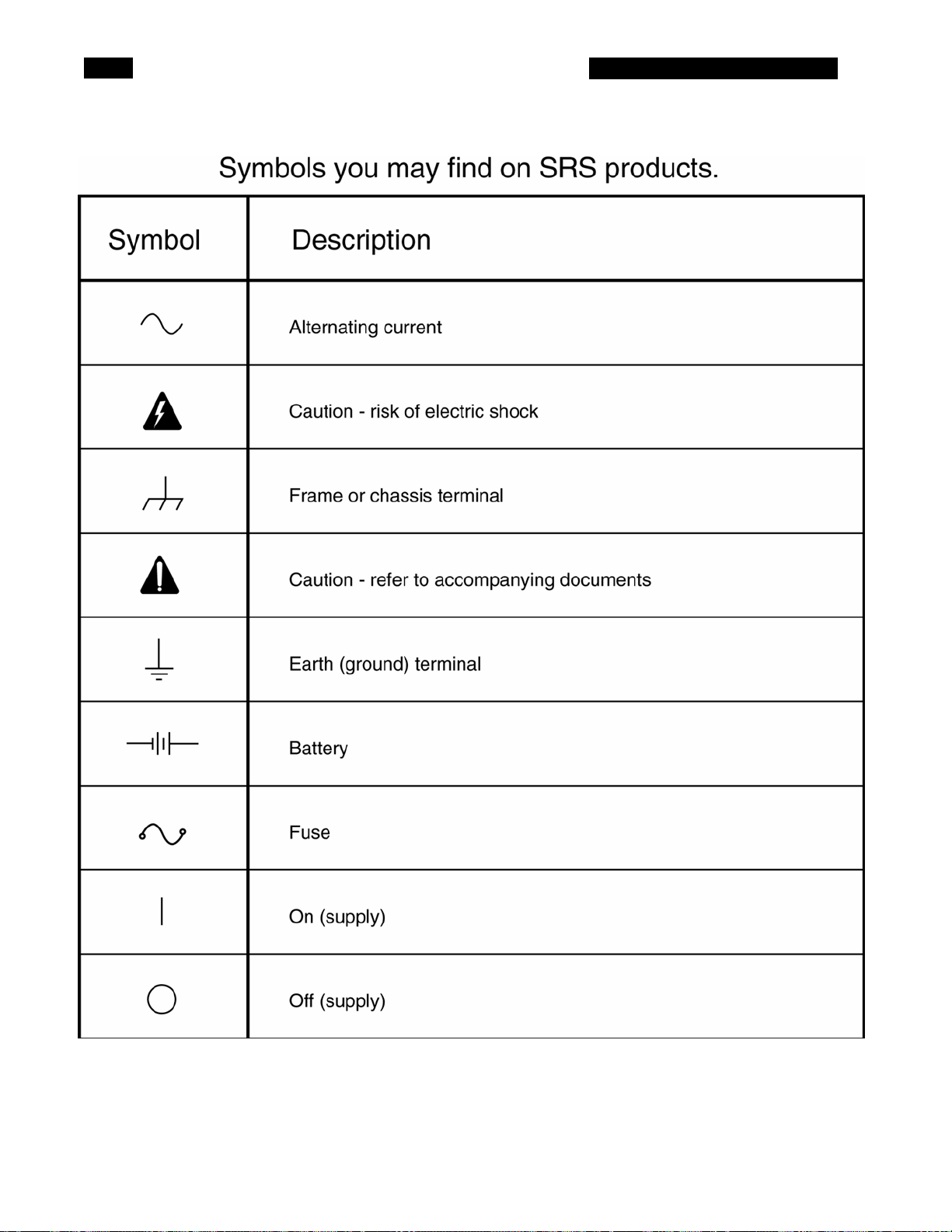
SAFETY AND PREPARATION FOR USE

WARNING

Dangerous voltages, capable of causing injury or death, are present in this instrument. Use extreme caution
whenever the instrument covers are removed. Do not remove the covers while the unit is plugged into a live
outlet.

CAUTION

This instrument may be damaged if operated with
the LINE VOLTAGE SELECTOR set for the wrong
AC line voltage or if the wrong fuse is installed.

LINE VOLTAGE SELECTION

The SR760 operates from a 100V, 120V, 220V, or
240V nominal AC power source having a line
frequency of 50 or 60 Hz. Before connecting the
power cord to a power source, verify that the LINE
VOLTAGE SELECTOR card, located in the rear
panel fuse holder, is set so that the correct AC
input voltage value is visible.

Conversion to other AC input voltages requires a
change in the fuse holder voltage card position
and fuse value. Disconnect the power cord, open
the fuse holder cover door and rotate the fuse-pull
lever to remove the fuse. Remove the small
printed circuit board and select the operating
voltage by orienting the printed circuit board so
that the desired voltage is visible when pushed
firmly into its slot. Rotate the fuse-pull lever back
into its normal position and insert the correct fuse
into the fuse holder.

LINE FUSE

Verify that the correct line fuse is installed before
connecting the line cord. For 100V/120V, use a 1
Amp fuse and for 220V/240V, use a 1/2 Amp fuse.

LINE CORD

The SR760 has a detachable, three-wire power
cord for connection to the power source and to a
protective ground. The exposed metal parts of the
instrument are connected to the outlet ground to
protect against electrical shock. Always use an
outlet which has a properly connected protective
ground.

SERVICE

Do not attempt to service or adjust this instrument
unless another person, capable of providing first
aid or resuscitation, is present.

Do not install substitute parts or perform any
unauthorized modifications to this instrument.
Contact the factory for instructions on how to
return the instrument for authorized service and
adjustment.

iii

SR760 FFT SPECTRUM ANALYZER

iv

SR760 FFT SPECTRUM ANALYZER

SPECIFICATIONS

FREQUENCY

Measurement Range 476 µHz to 100 kHz, baseband and zoomed.
Spans 191 mHz to 100 kHz in a binary sequence.
Center Frequency Anywhere within the measurement range subject to span and range limits.
Accuracy 25 ppm from 20°C to 40°C.
Resolution Span/400
Window Functions Blackman-Harris, Hanning, Flattop and Uniform.
Real-time Bandwidth 100 kHz

SIGNAL INPUT

Number of Channels 1
Input Single-ended or true differential
Input Impedance 1 MΩ, 15 pf
Coupling AC or DC
CMRR 90 dB at 1 kHz (Input Range < -6 dBV)
80 dB at 1 kHz (Input Range <14 dBV)
50 dB at 1 kHz (Input Range ≥ 14 dBV)
Noise 5 nVrms/√Hz at 1 kHz typical, 10 nVrms/√Hz max.
(-166 dBVrms/√Hz typ., -160 dBVrms/√Hz max.)

AMPLITUDE

Full Scale Input Range -60 dBV (1.0 mVpk) to +34 dBV (50 Vpk) in 2 dB steps.
Dynamic Range 90 dB typical
Harmonic Distortion No greater than -80 dB from DC to 100 kHz. (Input Range ≤ 0 dBV)

Spurious Input range ≥ -50 dBV:
No greater than -85 dB below full scale below 200 Hz.
No greater than -90 dB below full scale to 100 kHz.
Input Sampling 16 bit A/D at 256 kHz
Accuracy ± 0.3 dB ± 0.02% of full scale (excluding windowing effects).
Averaging RMS, Vector and Peak Hold.
Linear and exponential averaging up to 64k scans.

TRIGGER INPUT

Modes Continuous, internal, external, or external TTL.
Internal Level: Adjustable to ±100% of input scale.
Positive or Negative slope.
Minimum Trigger Amplitude: 10% of input range.
External Level: ±5V in 40 mV steps. Positive or Negative slope.
Impedance: 10 kΩ
Minimum Trigger Amplitude: 100 mV.
External TTL Requires TTL level to trigger (low<.7V, high>2V).
Post-Trigger Measurement record is delayed by 1 to 65,000 samples (1/512 to 127 time

records) after the trigger.
Delay resolution is 1 sample (1/512 of a record).
Pre-Trigger Measurement record starts up to 51.953 ms prior to the trigger.
Delay resolution is 3.9062 µs.
Phase Indeterminacy <2°

v

SR760 FFT SPECTRUM ANALYZER

DISPLAY FUNCTIONS

Display Real, imaginary, magnitude or phase spectrum.
Measurements Spectrum, power spectral density, time record and 1/3 octave.
Analysis Band, sideband, total harmonic distortion and trace math.
Graphic Expand Display expands up to 50x about any point in the display.

MARKER FUNCTIONS

Harmonic Marker Displays up to 400 harmonics of the fundamental.
Delta Marker Reads amplitude and frequency relative to defined reference.
Next Peak/Harmonic Locates nearest peak or harmonic to the left or right.
Data Tables Lists Y values of up to 200 user defined X points.
Limit Tables Automatically detects data exceeding up to 100 user defined upper and

lower limit trace segments.

GENERAL

Monitor Monochrome CRT. 640H by 480V resolution.
Adjustable brightness and screen position.
Interfaces IEEE-488, RS232 and Printer interfaces standard.
All instrument functions can be controlled through the IEEE-488 and RS232

interfaces. A PC keyboard input is provided for additional flexibility.

Hardcopy Screen dumps and table and setting listings to dot matrix and HP LaserJet

compatible printers. Data plots to HP-GL compatible plotters (via RS232 or
IEEE-488).

Disk 3.5 inch DOS compatible format, 720 kbyte capacity. Storage of data,

setups, data tables, and limit tables.
Power 60 Watts, 100/120/220/240 VAC, 50/60 Hz.
Dimensions 17"W x 6.25"H x 18.5"D
Weight 36 lbs.
Warranty One year parts and labor on materials and workmanship.

vi

SR760 FFT SPECTRUM ANALYZER

COMMAND LIST

VARIABLES g Trace0 (0), Trace1 (1), or Active Trace (-1)
i,j Integers
f Frequency (real)
x,y Real Numbers
s String

FREQUENCY page
SPAN (?) {i} 5-4 Set (Query) the Frequency Span to 100 kHz (19) through 191 mHz (0).
STRF (?) {f} 5-4 Set (Query) the Start Frequency to f Hz.
CTRF (?) {f} 5-4 Set (Query) the Center Frequency to f Hz.
OTYP (?) {i} 5-4 Set (Query) the number of bands in Octave Analysis to 15 (0) or 30 (1).
OSTR (?) {i} 5-4 Set (Query) the Starting Band in Octave Analysis to -2 ≤ i ≤ 35.
WTNG (?) {i} 5-4 Set (Query) the Weighting in Octave Analysis to none (0) or A-weighting (1).

MEASUREMENT page
MEAS (?) g {,i} 5-5 Set (Query) the Measurement Type to Spectrum (0), PSD (1), Time (2), or

DISP (?) g {,i} 5-5 Set (Query) the Display to LogMag (0),LinMag (1), Real (2), Imag (3), or Phase

UNIT (?) g {,i} 5-5 Set (Query) the Units to Vpk or deg (0),Vrms or rads (1), dBV (2), or dBVrms

VOEU (?) g {,i} 5-5 Set (Query) the Units to Volts (0), or EU (1).
EULB (?) g {,s} 5-5 Set (Query) the EU Label to string s.
EUVT (?) g {,x} 5-5 Set (Query) the EU Value to x EU/Volt.
WNDO (?) g {i} 5-5 Set (Query) the Window to Uniform (0), Flattop (1), Hanning (2), or BMH (3).

DISPLAY and MARKER page
ACTG (?) {i} 5-6 Set (Query) the Active Trace to trace0 (0) or trace1 (1).
FMTS (?) g {,i} 5-6 Set (Query) the Display Format to Single (0) or Dual (1) trace.
GRID (?) g {,i} 5-6 Set (Query) the Grid mode to Off (0), 8 (1), or 10 (2) divisions.
FILS (?) g {,i} 5-6 Set (Query) the Graph Style to Line (0) or Filled (1).
MRKR (?) g {,i} 5-6 Set (Query) the Marker to Off (0), On (1) or Track (2).
MRKW (?) g {,i} 5-6 Set (Query) the Marker Width to Norm (0), Wide (1), or Spot (2).
MRKM (?) g {,i} 5-6 Set (Query) the Marker Seeks mode to Max (0), Min (1), or Mean (2).
MRLK (?) {i} 5-6 Set (Query) the Linked Markers to Off (0) or On (1).
MBIN g,i 5-6 Move the marker region to bin i.
MRKX? 5-6 Query the Marker X position.
MRKY? 5-6 Query the Marker Y position.
MRPK 5-6 Move the Marker to the on screen max or min. Same as [MARKER MAX/MIN]

MRCN 5-6 Make the Marker X position the center of the span. Same as [MARKER

MRRF 5-6 Turns Marker Offset on and sets the offset equal to the marker position.
MROF (?) {i} 5-6 Set (Query) the Marker Offset to Off (0) or On (1).
MROX (?) {x} 5-6 Set (Query) the Marker Offset X value to x.
MROY (?) {x} 5-7 Set (Query) the Marker Offset Y value to x.
PKLF 5-7 Move the marker to the next peak to the left.
PKRT 5-7 Move the marker to the next peak to the right.
MSGS s 5-7 Display message s on the screen and sound an alarm.

SCALE page
TREF (?) g {,x} 5-8 Set (Query) the Top Reference to x.
BREF (?) g {,x} 5-8 Set (Query) the Bottom Reference to x.
YDIV (?) g {,x} 5-8 Set (Query) the Vertical Scale (Y/Div) to x.
AUTS g 5-8 AutoScale graph g. Similar to the [AUTO SCALE] key.
EXPD (?) g {,i} 5-8 Set (Query) the Horizontal Expand to no expand (5), 128, 64, 30, 15, or 8 bins

ELFT (?) g {,i} 5-8 Set (Query) the Left Bin when expanded to bin i.
XAXS (?) g {,i} 5-8 Set (Query) the X Axis scaling to Linear (0) or Log (1).

description

description

Octave (3).

(4).

(3).

description

key.

CENTER] key.

description

(4-0).

vii

SR760 FFT SPECTRUM ANALYZER

INPUT page description

ISRC (?) {i} 5-9 Set (Query) the Input to A (0) or A-B (1).
IGND (?) {i} 5-9 Set (Query) the Input Grounding to Float (0) or Ground (1).
ICPL (?) {i} 5-9 Set (Query) the Input Coupling to AC (0) or DC (1).
IRNG (?) {i} 5-9 Set (Query) the Input Range to i dBV full scale. -60 ≤ i ≤ 34 and i is even.
ARNG (?) {i} 5-9 Set (Query) the Auto Range mode to Manual (0) or Auto (1).
AOFF 5-9 Perform Auto Offset calibration.
AOFM (?) {i} 5-9 Set (Query) the Auto Offset Mode to Off (0) or On (1).
TMOD (?) {i} 5-9 Set (Query) the Trigger Mode to Cont (0), Int (1), Ext (2), or Ext TTL(3).
TRLV (?) {x} 5-9 Set (Query) the Trigger Level to x percent. -100.0 ≤ x ≤ 99.22.
TDLY (?) {i} 5-9 Set (Query) the Trigger Delay to i samples. -13300≤ i ≤ 65000.
ARMM (?) {i} 5-9 Set (Query) the Arming Mode to Auto (0) or Manual (1).
ARMS 5-9 Manually arm the trigger.

ANALYSIS page
ANAM (?) g {,i} 5-10 Set (Query) the real time Analysis to None (0), Harmonic (1), Sideband (2), or

CALC? g,i 5-10 Query result i (0 or 1) of the latest real time analysis.
FUND (?) g {,f} 5-10 Set (Query) the Harmonic Fundamental to frequency f Hz.
NHRM (?) g {,i} 5-10 Set (Query) the Number of Harmonics to 0 ≤ i ≤ 400.
NHLT 5-10 Move the Marker or Center Frequency to the next harmonic to the left.
NHRT 5-10 Move the Marker or Center Frequency to the next harmonic to the right.
SBCA (?) g {,f} 5-10 Set (Query) the Sideband Carrier to frequency f Hz.
SBSE (?) g {,f} 5-10 Set (Query) the Sideband Separation to f Hz.
NSBS (?) g {,i} 5-10 Set (Query) the Number of Sidebands to 0 ≤ i ≤ 200.
BSTR (?) g {,f} 5-10 Set (Query) the Band Start to frequency f Hz.
BCTR (?) g {,f} 5-10 Set (Query) the Band Center to frequency f Hz.
BWTH (?) g {,f} 5-11 Set (Query) the Band Width to f Hz.
TABL 5-11 Turn on Data Table display for the active trace.
DTBL (?) g {,i}{,f} 5-11 Set (Query) Data Table line i to frequency f.
DINX (?) {i} 5-11 Set (Query) Data Table index to i.
DINS 5-11 Insert a new line in the data table.
DIDT 5-11 Delete a line from the data table.
DLTB 5-11 Delete the entire data table.
LIMT 5-12 Turn on Limit Table display for the active trace.
TSTS (?) {i} 5-12 Set (Query) the Limit Testing to Off (0) or On (1).
PASF? 5-12 Query the results of the latest limit test. Pass=0 and Fail=1.
LTBL (?) g {,i} {j,f1,f2,y1,y2} 5-12 Set (Query) Limit Table line i to Xbegin (f1), Xend (f2), Y1 and Y2.
LINX (?) {i} 5-12 Set (Query) Limit Table index to i.
LINS 5-12 Insert a new line in the limit table.
LIDT 5-12 Delete a line from the limit table.
LLTB 5-12 Delete the entire limit table.
LARM (?) {i} 5-12 Set (Query) the Audio Limit Fail Alarm to Off (0) or On (1).

AVERAGING page
AVGO (?) {i} 5-13 Set (Query) Averaging to Off (0) or On (1).
NAVG(?) {i} 5-13 Set (Query) the Number of Averagesto 2 ≤ i ≤ 32000.
AVGT (?) {i} 5-13 Set (Query) the Averaging Type to RMS (0), Vector (1), or Peak Hold (2).
AVGM (?) {i} 5-13 Set (Query) the Averaging Mode to Linear (0) or Exponential (1).
OVLP (?) {x} 5-13 Set (Query) the Overlap to x percent. 0 ≤ x ≤ 100.0.

PLOT page
PLOT 5-14 Plot the entire graph (or graphs).
PTRC 5-14 Plot the trace (or traces) only.
PMRK 5-14 Plot the marker (or markers) only.
PTTL (?) {s} 5-14 Set (Query) the Plot Title to string s.
PSTL (?) {s} 5-14 Set (Query) the Plot Subtitle to string s.
PRSC 5-14 Print the screen. Same as the [PRINT] key.
PSET 5-14 Print the analyzer settings.
PLIM 5-14 Print the Limit Table of the active graph.
PDAT 5-14 Print the Data Table of the active graph.

SETUP page

OUTP (?) {i} 5-15 Set (Query) the Output Interface to RS232 (0) or GPIB (1).

description

Band (3).

description

description

description

viii

SR760 FFT SPECTRUM ANALYZER

OVRM (?) {i} 5-15 Set (Query) the GPIB Overide Remote state to Off (0) or On (1).
KCLK (?) {i} 5-15 Set (Query) the Key Click to Off (0) or On (1).
ALRM (?) {i} 5-15 Set (Query) the Alarms to Off (0) or On (1).
THRS (?) {i} 5-15 Set (Query) the Hours to 0≤ i ≤ 23.
TMIN (?) {i} 5-15 Set (Query) the Minutes to 0 ≤ i ≤ 59.
TSEC (?) {i} 5-15 Set (Query) the Seconds to 0 ≤ i ≤ 59.
DMTH (?) {i} 5-15 Set (Query) the Month to 1 ≤ 1 ≤ 12.
DDAY (?) {i} 5-15 Set (Query) the Day to 1 ≤ 1 ≤ 31.
DYRS (?) {i} 5-15 Set (Query) the Year to 0 ≤ 1 ≤ 99.
PLTM (?) {i} 5-15 Set (Query) the Plotter Mode to RS232 (0) or GPIB (1).
PLTB (?) {i} 5-15 Set (Query) the Plotter Baud Rate to 300 (0), 1200 (1), 2400 (2), 4800 (3),

9600 (4).

PLTA (?) {i} 5-15 Set (Query) the Plotter GPIB Address to 0 ≤ i ≤ 30.
PLTS (?) {i} 5-15 Set (Query) the Plot Speed to Fast (0) or Slow (1).
PNTR (?) {i} 5-15 Set (Query) the Trace Pen Number to 1 ≤ i ≤ 6.
PNGD (?) {i} 5-15 Set (Query) the Grid Pen Number to 1 ≤ i ≤ 6.
PNAP (?) {i} 5-15 Set (Query) the Alphanumeric Pen Number to 1 ≤ i ≤ 6.
PNCR (?) {i} 5-16 Set (Query) the Cursor Pen Number to 1 ≤ i ≤ 6.
PRNT (?) {i} 5-16 Set (Query) the Printer Type to Epson (0) or HP (1).

STORE AND RECALL FILE page
FNAM (?) {s} 5-17 Set (Query) the current File Name to string.
SVTR 5-17 Save the Active Trace Data to the file specified by FNAM.
SVST 5-17 Save the Settings to the file specified by FNAM.
RCTR 5-17 Recall the Trace Data from the file specified by FNAM to the active graph.
RCST 5-17 Recall the Settings from the file specified by FNAM.

MATH OPERATIONS page
CSEL (?) {i} 5-18 Set (Query) the Operation to +, -, x, /, log, √ (0-5).
COPR 5-18 Start the calculation.
CARG (?) {i} 5-18 Set (Query) the Argument type to Constant (0), w (1), or Other Graph (2).
CONS (?) {x} 5-18 Set (Query) the Constant Argument to x.
CMRK 5-18 Set the Constant Argument to the Y value of the marker.

FRONT PANEL CONTROLS page
STRT 5-19 Start data acquisition. Same as [START] key.
STCO 5-19 Pause or Continue data acquisition. Same as [PAUSE CONT] key.
PRSC 5-19 Print the screen. Same as [PRINT] key.
ACTG (?) {i} 5-19 Set (Query) the Active Trace to trace0 (0) or trace1 (1). Similar to [ACTIVE

ARNG (?) {i} 5-19 Set (Query) the Auto Range mode to Manual (0) or Auto (1). Similar to [AUTO

AUTS 5-19 AutoScale the graph. Same as the [AUTO SCALE] key.

DATA TRANSFER page
SPEC? g {,i} 5-20 Query the Y value of bin 0 ≤ i ≤ 399.
BVAL? g, i 5-20 Query the X value of bin 0 ≤ i ≤ 399.
SPEB? g 5-20 Binary dump the entire trace g.
BDMP (?) g, {,i} 5-21 Set (Query) the auto binary dump mode for trace g.

INTERFACE page
*RST 5-22 Reset the unit to its default configurations.
*IDN? 5-22 Read the SR760 device identification string.
LOCL(?) {i} 5-22 Set (Query) the Local/Remote state to LOCAL (0), REMOTE (1), or LOCAL

OVRM (?) {i} 5-22 Set (Query) the GPIB Overide Remote state to Off (0) or On (1).

STATUS page
*CLS 5-23 Clear all status bytes.
*ESE (?) {i} {,j} 5-23 Set (Query) the Standard Status Byte Enable Register to the decimal value i

*ESR? {i} 5-23 Query the Standard Status Byte. If i is included, only bit i is queried.
*SRE (?) {i} {,j} 5-23 Set (Query) the Serial Poll Enable Register to the decimal value i (0-255).
*STB? {i} -23 Query the Serial Poll Status Byte. If i is included, only bit i is queried.

description

description

description

TRACE] key.

RANGE] key.

description

description

LOCKOUT (2).

description

(0-255).

ix

SR760 FFT SPECTRUM ANALYZER

*PSC (?) {i} 5-23 Set (Query) the Power On Status Clear bit to Set (1) or Clear (0).
ERRE (?) {i} {,j} 5-23 Set (Query) the Error Status Enable Register to the decimal value i (0-255).
ERRS? {i} 5-23 Query the Error Status Byte. If i is included, only bit i is queried.
FFTE (?) {i} {,j} 5-23 Set (Query) the FFT Status Enable Register to the decimal value i (0-255).
FFTS? {i} 5-23 Query the FFT Status Byte. If i is included, only bit i is queried.

STATUS BYTE DEFINITIONS

SERIAL POLL STATUS BYTE (6-24)

name usage

bit
0 SCN No measurements in progress
1 IFC No command execution in progress
2 ERR Unmasked bit in error status byte set
3 FFT Unmasked bit in FFT status byte set
4 MAV The interface output buffer is non-empty
5 ESB Unmasked bit in standard status byte

set
6 SRQ SRQ (service request) has occurred
7 Unused

STANDARD EVENT STATUS BYTE (6-25)

name usage

bit
0 INP Set on input queue overflow
1 Limit Fail Set when a limit test fails
2 QRY Set on output queue overflow
3 Unused
4 EXE Set when command execution error

occurs
5 CMD Set when an illegal command is

received
6 URQ Set by any key press or knob rotation
7 PON Set by power-on

FFT STATUS BYTE (6-25)

name usage

bit
0 Triggered Set when a time record is triggered
1 Prn/Plt Set when a printout or plot is completed
2 NewData 0 Set when new data is available for trace 0
3 NewData 1 Set when new data is available for trace 1
4 Avg Set when a linear average is completed
5 AutoRng Set when auto range changes the range
6 High Voltage Set when high voltagedetected at input
7 Settle Set when settling is complete

ERROR STATUS BYTE (6-26)

name usage

bit

0 Prn/Plt Err Set when an printing or plotting error

occurs
1 Math Error Set when an internal math error occurs
2 RAM Error Set when RAM Memory test finds an error
3 Disk Error Set when a disk error occurs
4 ROM Error Set when ROM Memory test finds an error
5 A/D Error Set when A/D test finds an error
6 DSP Error Set when DSP test finds an error
7 Overload Set when the signal input overloads

x

YOUR FIRST MEASUREMENT

This sample measurement is designed to acquaint
the first time user with the SR760 Spectrum
Analyzer. Do not be concerned that your
measurement does not exactly agree with this
exercise. The focus of this measurement exercise
is to learn how to use the instrument.

There are two types of front panel keys which will
be referenced in this section. Hardkeys are those
keys with labels printed on them. Their function is
determined by the label and does not change.
Hardkeys are referenced by brackets like this ­[HARDKEY]. The softkeys are the six gray keys
along the right edge of the screen. Their function
is labelled by a menu box displayed on the screen
next to the key. Softkey functions change
depending upon the situation. Softkeys will be
referenced as the <Soft Key> or simply the Soft
Key.

Hardkeys

The keypad consists of five groups of hardkeys.
The ENTRY keys are used to enter numeric
parameters which have been highlighted by a
softkey. The MENU keys select a menu of
softkeys. Pressing a menu key will change the
menu boxes which are displayed next to the
softkeys. Each menu groups together similar
parameters and functions. The CONTROL keys
start and stop actual data acquisition, select the
marker and toggle the active trace the display.
These keys are not in a menu since they are used
frequently while displaying any menu. The
SYSTEM keys output the screen to a printer and
display help messages. These keys can also be
accessed from any menu. The MARKER keys
determine the marker mode and perform various
marker functions. The marker functions can be
accessed from any menu.

GETTING STARTED

Softkeys

The SR760 has a menu driven user interface. The
6 softkeys to the right of the video display have
different functions depending upon the information
displayed in the menu boxes at the right of the
video display. In general, the softkeys have two
uses. The first is to toggle a feature on and off or
to choose between settings. The second is to
highlight a parameter which is then changed using
the knob or numeric keypad. In both cases, the
softkey affects the parameter which is displayed
adjacent to it.

Knob

The knob is used to adjust parameters which have
been highlighted using the softkeys. Most numeric
entry fields may be adjusted with the knob. In
addition, functions such as display zooming and
scrolling use the knob as well. In these cases, the
knob function is selected by the softkeys. The
[MARKER] key, which can be pressed at any time,
will set the knob function to scrolling the marker.

Example Measurement

This measurement is designed to investigate the
spectrum of a 1 kHz sine wave. You will need a
function generator capable of providing a 1 kHz
sine wave at a level of 100 mV to 1 V, such as the
SRS DS345. The actual settings of the generator
are not important since you will be using the
SR760 to measure and analyze its output. Choose
a generator which has some distortion (at least ­70 dBc) or use a square or triangle wave.

Specifically, you will measure the spectrum of the
sine wave, measure its frequency, and measure
its harmonic distortion.

1-1

GETTING STARTED

ANALYZING A SINE WAVE

1. Turn the analyzer on while holding down the
[<-] (backspace) key. Wait until the power­on tests are completed.

2. Turn on the generator, set the frequency to
1 kHz and the amplitude to approximately 1
Vrms.

Connect the generator's output to the A

input of the analyzer.

3. Press [AUTO RANGE]

4. Press the <Span> softkey to highlight the
span. Use the knob to adjust the span to

6.25 kHz.

You can also use the [SPAN UP] and

[SPAN DOWN] keys to adjust the span.

5. Press [MARKER MAX/MIN]

6. Press [MARKER]

Use the knob to move the marker around.

Take a look at some of the harmonics.

7. Let's measure the frequency exactly.

Decrease the span to 1.56 kHz using the

<Span> key and knob, the [SPAN DOWN]
key or by entering the span numerically.

Press [MARKER MAX/MIN]

Press [MARKER CENTER]

When the power is turned on with the backspace
key depressed, the analyzer returns to its default
settings. See the Default Settings list in the Menu
section for a complete listing of the settings.

The input impedance of the analyzer is 1 MΩ. The
generator may require a terminator. Many
generators have either a 50 Ω or 600 Ω output
impedance. Use the appropriate feedthrough
termination if necessary. In general, not using a
terminator means that the output amplitude will
not agree with the generator setting and the
distortion may be greater than normal.

Since the signal amplitude may not be set
accurately, let the analyzer automatically set its
input range to agree with the actual generator
signal. Note that the range readout at the bottom
of the screen is displayed in inverse when the
autoranging is on.

Set the span to display the 1 kHz signal and its
first few harmonics.

You can also use the numeric keypad to enter the
span. In this case, the span will be rounded to the
next largest allowable span.

This centers the marker region around the largest
data point on the graph. The marker should now
be on the 1 kHz signal. The marker readout above
the graph displays the frequency and amplitude of
the signal.

The [MARKER MAX/MIN] key can also be
configured to search for the minimum point on the
graph.

Pressing the [MARKER] key allows the knob to
adjust the marker position. The Span Menu box
becomes unhighlighted. A box is drawn around
the marker readout to indicate that the knob will
move the marker.

This isolates the 1 kHz fundamental frequency.

Move the marker to the peak at 1 kHz.

This sets the span center frequency to the marker
frequency. The signal will be at the center of the

1-2

8. Decrease the span to 97.5 Hz using the

<Span> key and knob, the [SPAN DOWN]
key or by entering the span numerically.

9. Press [MARKER MAX/MIN]

10. Press [AUTO SCALE]

11. Press [ANALYZE]

Press <Harmonic>

12. Press <Next Harmonic Right>

Use the <Next Harmonic Right> and
<Next Harmonic Left> keys to investigate

the harmonics of the signal.

13. Press [FREQ]

Press <Full Span>

Press [AUTO SCALE]

14. Press <Start Freq.>

Now adjust the span to 12.5 kHz using the

GETTING STARTED

span. Further adjustments to the span will keep
the center frequency fixed.

You may notice that the spectrum takes a while to
settle down at this last span. This is because the
frequency resolution is 1/400 of the span or
244 mHz. This resolution requires at least

4.096 seconds of time data. Note that the Settling
indicator at the lower right corner of the display
will stay on while the data settles.

This centers the marker more accurately. The
frequency of the signal can now be read with
244 mHz resolution.

This key adjusts the graph scale and top
reference to display the entire range of the data.
You can press this key at any time to optimize the
graph display.

Display the Analysis menu.

Select Harmonic analysis. The menu displays the
harmonic analysis menu. Notice that the
fundamental frequency (first menu box) has been
set to the frequency of the marker.

We used a narrow span to get an accurate
reading of the fundamental signal frequency. We
will use this measurement of the fundamental to
accurately locate the harmonics.

The harmonic measurement readout at the upper
left corner of the graph is under range because
the span is not wide enough to include any
harmonics.

This centers the span around the second
harmonic (approx. 2 kHz). You are now making
an accurate measurement of the 2nd harmonic
content of the signal.

With this narrow span, the harmonics should be
easily visible.

Let's have the analyzer measure the distortion for
us. First return to full span by displaying the
frequency menu and choosing full span.

Return the graph to a scale where the
fundamental is on screen.

This highlights the Start Frequency menu box. It
also fixes the start frequency when the span is
adjusted.

Reduce the span to resolve the first few

1-3

GETTING STARTED

<Span> key and knob, the [SPAN DOWN]
key or by entering the span numerically.

15. Press [ANALYZE]

Press <Harmonic>

16. Press <# Harmonics>

Press [1] [1] <Enter>

17. Now let's measure some harmonics using
the reference marker.

Press <Return>

Press <None>

Press [MARKER MAX/MIN]

Press [MARKER REF]

Press [MARKER]

Use the knob to measure the harmonic

levels relative to the fundamental.

18. Press [MARKER REF]

harmonics of the signal.

Display the Analysis menu.

Choose Harmonic analysis. (It should still be on
from before.) The fundamental frequency should
still be accurately set.

Highlight the number of harmonics menu box.

Enter 11 for the number of harmonics.

Notice that harmonic markers (little triangles)
appear on top of all of the harmonic peaks. These
indicate which data points are used in the
harmonic calculations.

The harmonic calculations are displayed in the
upper left corner of the graph. The top reading is
the harmonic level (absolute units) and the lower
reading is the distortion (harmonic level divided by
the fundamental level).

Return the menu display to the main Analysis
menu.

Choose No analysis. This turns off the harmonic
indicators and calculations.

This moves the marker to the fundamental peak.

This sets the marker reference or offset to the
frequency and amplitude of the fundamental. The
marker readout above the graph now reads
relative to this offset. This is indicated by the ∆ in
front of the marker readout. A small star shaped
symbol is located at the screen location of the
reference.

This allows the knob to move the marker.

The marker readout is now relative to the
reference or fundamental level.

Pressing [MARKER REF] again removes the
marker offset.

This concludes this measurement example. You
should have a good feeling for the basic operation
of the menus, knob and numeric entry, and
marker movement and measurements.

1-4

SECOND MEASUREMENT EXAMPLE

This sample measurement is designed to further
acquaint the user with the SR760 Spectrum
Analyzer. Do not be concerned that your
measurement does not exactly agree with this
exercise. The focus of this measurement exercise
is to learn how to use the instrument.

There are two types of front panel keys which will
be referenced in this section. Hardkeys are those
keys with labels printed on them. Their function is
determined by the label and does not change.
Hardkeys are referenced by brackets like this ­[HARDKEY]. The softkeys are the six gray keys
along the right edge of the screen. Their function
is labelled by a menu box displayed on the screen
next to the key. Softkey functions change
depending upon the situation. Softkeys will be
referenced as the <Soft Key> or simply the Soft
Key.

GETTING STARTED

The Measurement

This measurement is designed to investigate the
noise of an audio amplifier. You will need an audio
frequency amplifier such as the SRS SR560. You
will also need a function generator capable of
providing a 1 kHz sine wave at a level of 100 mV
to 1 V such as the SRS DS345.

Specifically, you will measure the output
signal/noise ratio of the amplifier and its input
noise level.

1-5

GETTING STARTED

MEASURING AMPLIFIER NOISE

1. Turn the analyzer on while holding down the
[<-] (backspace) key. Wait until the power­on tests are completed.

2. Turn on the generator, set the frequency to
1 kHz and amplitude to approximately 1
Vrms.

Connect the generator's output to the input

of the amplifier. Turn on the amplifier and
set its gain to at least 20 dB. Connect the
amplifier output to the A input of the
analyzer.

3. Press [AUTO RANGE]

4. Press [SPAN DOWN] until the span is

6.25 kHz

5. Press [AUTO SCALE]

6. Press [MAX/MIN]

7. Press [MARKER REF]

Use the knob to move the marker to a

region that is representative of the noise
floor.

7. Press [MARKER REF] again

8. Press {MEAS]

Press <Measure Menu>

Press <PSD>

When the power is turned on with the backspace
key depressed, the analyzer returns to its default
settings. See the Default Settings list in the Menu
section for a complete listing of the settings.

The input impedance of the analyzer is 1 MΩ. The
generator and/or amplifier may require a
terminator. Many instruments have either a 50 Ω
or 600 Ω output impedance. Use the appropriate
feedthrough termination if necessary. In general,
not using a terminator means that the output
amplitude will not agree with the instrument
setting and the distortion may be greater than
normal.

Since the signal amplitude may not be set
accurately, let the analyzer automatically set its
input range to the actual signal.

Set the span to display the 1 kHz signal and its
first few harmonics.

Set the graph scaling to display the entire range
of the data.

Move the marker to the signal peak (1 kHz). The
marker should read an amplitude equal to the
generator output times the amplifier gain.

This turns on the marker offset and sets the
reference marker to the current marker position.
From now on, the marker will now read relative to
the signal peak. A ∆ is displayed before the
marker readout to indicate that the reading is
relative. A small star symbol is located on the
graph at the marker offset position.

The marker is now providing a direct reading of
the signal to noise ratio. Remember, this is the
S/N for the generator/amplifier combination. It
may be that the amplifier is better than the
generator. To check this, turn off the generator. If
the noise floor is lower, then the generator is
determining the output S/N.

The [MARKER REF] key toggles the marker offset
on and off. We now want to turn the offset off.

Display the Measure menu.

Choose the Measurement type menu.

Select Power Spectral Density. The PSD
approximates the amplitude of the signal within a
1 Hz bandwidth located at each frequency bin.

1-6

9. Press [AVERAGE]

Press <Average Mode>

10. Press <Number of Averages>

Press [2] [0] <Enter>

11. Press <Averaging>

12. Press [MARKER]

Use the knob to move the marker to a

region representative of the noise floor.

13. Press [MEAS]

Press <Units Menu>

Press <Volts RMS>

14. Disconnect the generator output from the

amplifier. Leave the amplifier input
terminated.

GETTING STARTED

This allows measurements taken with different
linewidths (spans) to be compared.

To get a better measurement of noise, a little
averaging can help.

Display the Average menu.

Select Exponential averaging.

Highlight the Number of Averages menu box.

Enter 20 averages.

Turn averaging on. Notice how the noise floor
approaches a more stable value. We are using
RMS averaging to determine the actual noise
floor. See the section on Averaging for a
discussion of the different types of averaging.

The [MARKER] key allows the knob to move the
marker.

The Marker reading should be in dBV/√Hz. This is
the output noise amplitude at the marker
frequency, normalized to a 1 Hz bandwidth. To
generalize to other bandwidths, multiply by the
square root of the bandwidth. This approximation
only holds if the noise is Gaussian in nature.

Display the Measure menu.

Choose the Units menu.

Select Volts RMS as the display units.

The marker now reads in Volts RMS /√Hz. This is
a typical way of specifying amplifier input noise
levels.

Now we are measuring the amplifier's output
noise with a shorted input. If you take the noise
measurement and divide by the amplifier gain,
then you will have the amplifier's input noise at the
frequency of the marker reading.

An FFT is a convenient tool for measuring
amplifier noise spectra since the noise at many
frequencies can be determined in a single
measurement.

1-7

GETTING STARTED

USING TRIGGERS AND THE TIME RECORD

This sample measurement is designed to acquaint
the user with the triggering capabilities of the
SR760 Spectrum Analyzer. Do not be concerned
that your measurement does not exactly agree
with this exercise. The focus of this measurement
exercise is to learn how to use the instrument.

There are two types of front panel keys which will
be referenced in this section. Hardkeys are those
keys with labels printed on them. Their function is
determined by the label and does not change.
Hardkeys are referenced by brackets like this ­[HARDKEY]. The softkeys are the six gray keys
along the right edge of the screen. Their function
is labelled by a menu box displayed on the screen
next to the key. Softkey functions change
depending upon the situation. Softkeys will be
referenced as the <Soft Key> or simply the Soft
Key.

The Measurement

This measurement is designed to investigate the
trigger and time record. You will need a function
generator capable of providing a 100 µs wide
pulse at 250 Hz with an amplitude of 1 V. The
output should have a DC level of 0V.

Specifically, you will measure the output spectrum
when the signal is triggered. In addition, the trigger
delay will be used to delay the signal within the
time record.

Make sure that you have read "The Time Record"
in the Analyzer Basics section before trying this
exercise.

1-8

TRIGGERING THE ANALYZER

1. Turn the analyzer on while holding down the

[<-] (backspace) key. Wait until the power­on tests are completed.

2. Turn on the generator and choose a pulsed

output waveform. Set the frequency to
250 Hz, the pulse width to 100 µs and the
amplitude to approximately 1 V. Make sure
that the DC level of the output is near 0V.

Connect the generator's output to the A

input of the analyzer.

3. Press [INPUT]

Press <Coupling> to choose DC

Press <Input Range>

Press [4] <dBV>

4. Press [DISPLAY]

Press <Format> to choose Up/Dn

5. Press [MEAS]

Press <Measure Menu>

Press <Time Record>

Press <Return>

Press <Display Menu>

Press <Linear Mag.>

6. Press [INPUT]

Press <Trigger Menu>

Press <Trigger> to select Internal

Press <Trigger Level>

Press [.] [5] <Volts>

Press [AUTO SCALE]

GETTING STARTED

When the power is turned on with the backspace
key depressed, the analyzer returns to its default
settings. See the Default Settings list in the Menu
section of this manual for a complete listing of the
settings.

The input impedance of the analyzer is 1 MΩ. The
generator may require a terminator. Many
generators have either a 50 Ω or 600 Ω output
impedance. Use the appropriate feedthrough
termination if necessary. In general, not using a
terminator only means that the output amplitude
will not agree with the generator setting and the
distortion may be greater than normal.

Let's choose DC coupling and an input range that
doesn't overload.

Set the input range to 4 dBV. Adjust the pulse
amplitude so that no overloads occur.

Show two traces.

We will show the time record on the upper trace.

Go to the Measure menu to choose Time Record.

Let's show the time record on a linear scale.

Now set up the trigger.

Trigger on the signal itself.

The input is a 1 V pulse so set the trigger level to

0.5 V.

The upper trace should display the pulse
waveform at the left edge. Auto scale will set the
display limits automatically. Remember that we
are displaying the magnitude of the signal. Any
negative portion of the signal will be folded back

1-9

GETTING STARTED

7. Press [MEAS]

Press <Window Menu>

Press <Uniform>

Press [ACTIVE TRACE]

Press [AUTO SCALE]

8. Press <Hanning>

9. Press [INPUT]

Press <Trigger Menu>

Press <Trigger Delay>

Press [2] [5] [6] <Samples>

10. Press [4] [7] [5] <Samples>

11. Press <Trigger> to select Continuous

around zero and appear as a positive magnitude.

Because the pulse is much shorter than the time
record, we need to use the Uniform window. The
other window functions taper to zero at the start
and end of the time record. Always be aware of
the effect windowing has on the FFT of thetime
record.

There should now be a spectrum on the lower
trace. Use [AUTO SCALE] to set the display.

The spectrum you see is the sinx/x envelope of a
rectangular pulse. The zeroes in the spectrum
occur at the harmonics of 1/pulse width (1/100µs
or 10 kHz).

Now choose the Hanning window. Notice how the
spectrum goes away. We can get the spectrum
back by delaying the time record relative to the
trigger so that the pulse is positioned in the center
of the time record.

Go back to the Trigger submenu.

Highlight the Trigger Delay menu box.

Enter 256 samples of delay. Because the pulse
repetition rate is 250 Hz, the period between
pulses is exactly equal to one time record. So
setting the delay to half of a time record will place
the pulse at the middle of the record.

Remember that the time record only displays the
first 400 points (out of 512) so that the middle of
the record is not the middle of the display trace.

The spectrum should reappear on the lower trace.
This is because windowing preserves the central
part of the time record.

Let's delay the signal some more. Now we've
delayed the time record by almost a full period.
The pulse is now near the end of the time record.

Notice how the spectrum is greatly attenuated.
This is the effect of the window function
attenuating the start of the timer record.

Now if we go to continuous triggering, the time
record becomes unstable. The spectrum is also
unstable because of the windowing. Some time
records place the pulse at the middle, some at the
ends.

1-10

12. Press [MEAS]

Press <Window>

Press <Uniform>

GETTING STARTED

If we set the window back to Uniform, we find that
the spectrum does not vary with the position of the
pulse within the time record.

1-11

GETTING STARTED

USING THE DISK DRIVE

The disk drive on the SR760 may be used to store
3 types of files.

1. Data File

This includes the data in the active trace,

the measurement and display type, the
units and the graph scaling. In addition,
the associated data and limit tables are
stored in this file as well. Data files may be
recalled into either trace0 or trace1.

2. ASCII Data File

This file saves the data in the active trace

in ASCII format. These files may not be
recalled to the display. This format is
convenient when transferring data to a PC
application.

3. Settings File

This files stores the analyzer settings.

Recalling this file will change the analyzer
setup to that stored in the file.

The disk drive uses double-sided, double density
(DS/DD) 3.5" disks. The disk capacity is 720k. The
SR760 uses the DOS format. A disk which was
formatted on a PC or PS2 (for 720k) may be used.
Files written by the SR760 may be copied or read
on a DOS computer.

Data files can store data in either binary or ascii
format. Binary format uses less disk space. Ascii
format allows trace data to be read by other
programs using a PC.

There are two types of front panel keys which will
be referenced in this section. Hardkeys are those
keys with labels printed on them. Their function is
determined by the label and does not change.
Hardkeys are referenced by brackets like this ­[HARDKEY]. The softkeys are the six gray keys
along the right edge of the screen. Their function
is labelled by a menu box displayed on the screen
next to the key. Softkey functions change
depending upon the situation. Softkeys will be
referenced as the <Soft Key> or simply the Soft
Key.

The Measurement

This measurement is designed to familiarize the
user with the disk drive. We will use a function
generator to provide an input signal so that there
is some data to save and recall. Use any function
generator capable of providing a 1 kHz sine wave
at a level of 100 mV to 1 V.

Specifically, you will save and recall a data file and
a settings file.

1-12

STORING AND RECALLING DATA

1. Turn the analyzer on while holding down the

[<-] (backspace) key. Wait until the power­on tests are completed.

2. Turn on the generator, set the frequency to

1 kHz and amplitude to approximately 1
Vrms.

Connect the generator's output to the A

input of the analyzer.

3. Press [AUTO RANGE]

4. Press [SPAN DOWN] until the span is

6.25 kHz

5. Press [AUTO SCALE]

6. Press [PAUSE CONT]

7. Put a blank double-sided, double density

(DS/DD)3.5" disk into the drive.

8. Press [STORE RECALL]

Press <Disk Utilities>

Press <Format Disk>

9. Press <Return>

Press <Save Data>

10. Press <File Name>

Press [ALT]

Press [D] [A] [T] [A] [1] <Enter>

When the power is turned on with the backspace

key depressed, the analyzer returns to its default
settings. See the Default Settings list in the Menu
section for a complete listing of the settings.

The input impedance of the analyzer is 1 MΩ. The

generator may require a terminator. Many
generators have either a 50 Ω or 600 Ω output
impedance. Use the appropriate feedthrough
termination if necessary. In general, not using a
terminator means that the output amplitude will
not agree with the generator setting and the
distortion may be greater than normal.

Since the signal amplitude may not be set

accurately, let the analyzer automatically set its
input range to actual signal.

Set the span to display the 1 kHz signal and its

first few harmonics.

Set the graph scaling to display the entire range

of the data.

Stop data acquisition. The graph on the screen is

the one we want to save. (You can actually save
graphs while the analyzer is running.)

Use a blank if disk if possible, otherwise any disk

that you don't mind formatting will do. Make sure
the write protect tab is off.

Let's format this disk.

Display the Store and Recall menu.

Choose Disk Utilities.

Make sure that the disk does not contain any
information that you want. Formatting the disk
takes about a minute.

Go back to the main Store and Recall menu.

Display the Save Data menu.

Now we need a file name.

[ALT] lets you enter the letter characters printed
below each key. The numbers and backspace
function as normal.

Enter a file name such as DATA1 (or any legal
DOS file name).

GETTING STARTED

1-13

GETTING STARTED

11. Press <Save Data>

12. Press <Catalog>

13. Press <File Name>

Press [ALT]

Press [D] [A] [T] [A] [2] <Enter>

Press <Save Data>

14. Press <Return>

Press [START]

Remove the input signal cable or turn off the

generator.

15. Press <Recall Data>

Press <Catalog>

16. Press [MARKER]

17. Press <Recall Data>

18. Press [DISPLAY]

Press <Format>

Press [ACTIVE TRACE]

19. Press [START]

This saves the active trace data to disk using the

file name specified above.

Display the disk catalog. This display lists all of

the files on the disk.

Save the data again using a new file name. This

way you can have multiple files in the disk
catalog.

Go back to the main Store and Recall menu.

Resume data acquisition. The graph should be
live again.

Now we have a spectrum which is different from
the one we just saved. Recalling the data from
disk will restore the graph to what it was.

Display the Recall Data menu.

Display the disk catalog. The 2 files which you just
saved should be listed.

Pressing the [MARKER] key allows the knob to

adjust the marker. When the disk catalog is
displayed, the marker highlights a file. Use the
knob to choose a file to recall.

This recalls the data file from disk and displays it

on the active graph. Data acquisition is stopped
so that the graph is not updated. The file name is
displayed below the graph.

The marker may be moved on the recalled graph
to read specific data points. The graph scaling
may also be changed.

Show the Display menu.

Choose the Up/Dn dual trace display format.

Make trace1 active (the lower graph). The active
graph has a highlighted label at its upper right.

This restarts data acquisition, but only for the

active trace (trace1). The recalled trace on graph
0 is still displayed. To restart data acquisition on
trace0, press [ACTIVE TRACE] to make trace0
active and then [START].

1-14

GETTING STARTED

STORING AND RECALLING SETTINGS

1. Turn the analyzer on while holding down the

[<-] (backspace) key. Wait until the power­on tests are completed.

2. Press [SPAN DOWN] a number of times to

change the span.

Press [INPUT]

Press <Coupling>

3. Press [STORE RECALL]

Press <Save Settings>

4. Press <File Name>

Press [ALT]

Press [T] [E] [S] [T] [1] <Enter>

5. Press <Save Settings>

6. Press [SPAN UP] a number of times to

change the span.

Press [INPUT]

Press <Coupling>

7. Press [STORE RECALL]

Press <Recall Settings>

Press <Catalog>

8. Press [MARKER]

9. Press <Recall Settings>

When the power is turned on with the backspace

key depressed, the analyzer returns to its default
settings. See the Default Settings list in the Menu
section for a complete listing of the settings.

Change the analyzer setup so that we have a

non-default setup to save.

Show the Input menu.

Choose DC coupling.

Display the Store and Recall menu.

Choose the Save Settings menu.

Now we need a file name.

[ALT] lets you enter the letters printed below each
key. The numbers and backspace function as
normal.

Enter a file name such as TEST1 (or any legal
DOS file name).

Save the analyzer setup to disk using the file

name specified above.

Change the analyzer setup again.

Show the Input menu.

Choose AC coupling.

Now let's recall the analyzer setup that we just
saved.

Display the Store and Recall menu.

Choose the Recall Settings menu.

Display the disk catalog listing. Note that data files
have the type DAT and setting files have the type
SET.

Pressing the [MARKER] key allows the knob to

adjust the marker. When the disk catalog is
displayed, the marker highlights a file. Use the
knob to choose the file TEST1 to recall. (Or use
the <File Name> key to enter the file name.)

This recalls the settings from the file TEST1. The

analyzer settings are changed to those stored in

1-15

GETTING STARTED

TEST1. The span and input coupling should be
the same as those in effect when you created the
file.

1-16

USING DATA TABLES

A data table reports the Y values for user listed X­axis values. For example, the entries could be a
set of harmonic frequencies which need to be
measured. The data table is a convenient way to
measure the data values at various points without
moving the marker around and manually recording
the answers. To generate a printed report of the
measurement, the data table may be printed using
the Plot menu.

Each trace has its own data table though only the
table associated with the active trace is on and
displayed at any time.

Data tables are saved along with the trace data
when data is saved to disk.

Data tables are not stored in non-volatile memory
and are not retained when the power is turned off.

Remember that the values in the table do not have
units associated with them. An X location of 10
kHz is stored as 10 k and a Y value of -20 dBV is
reported as simply -20. The Y values come directly
from the graph so it is important to use the proper
display units to get consistent data table readings.

There are two types of front panel keys which will
be referenced in this section. Hardkeys are those
keys with labels printed on them. Their function is
determined by the label and does not change.
Hardkeys are referenced by brackets like this ­[HARDKEY]. The softkeys are the six gray keys
along the right edge of the screen. Their function
is labelled by a menu box displayed on the screen
next to the key. Softkey functions change
depending upon the situation. Softkeys will be
referenced as the <Soft Key> or simply the Soft
Key.

GETTING STARTED

The Measurement

This measurement is designed to familiarize the
user with the data tables. We will use a function
generator to provide an input signal so that there
is some data to report. Use any function generator
capable of providing a 1 kHz sine wave at a level
of 100 mV to 1 V.

Specifically, you will generate a data table to
measure some harmonics as well as the noise
floor.

1-17

GETTING STARTED

DATA TABLES

1. Turn the analyzer on while holding down the
[<-] (backspace) key. Wait until the power­on tests are completed.

2. Turn on the generator, set the frequency to
1 kHz and amplitude to approximately 1
Vrms.

Connect the generator's output to the A

input of the analyzer.

3. Press [AUTO RANGE]

4. Press [SPAN DOWN] until the span is

6.25 kHz

5. Press [AUTO SCALE]

6. Press [ANALYZE]

Press <Data Table>

7. Press [MARKER MAX/MIN]

Press <X Value>

Press [MARKER ENTRY]

8. Press <Table Index>

Press [1] <Enter>

9. Press [MARKER]

Use the knob to locate the 2nd harmonic of

the signal.

Press <X Value>

When the power is turned on with the backspace

key depressed, the analyzer returns to its default
settings. See the Default Settings list in the Menu
section for a complete listing of the settings.

The input impedance of the analyzer is 1 MΩ. The

generator may require a terminator. Many
generators have either a 50 Ω or 600 Ω output
impedance. Use the appropriate feedthrough
termination if necessary. In general, not using a
terminator means that the output amplitude will
not agree with the generator setting and the
distortion may be greater than normal.

Since the signal amplitude may not be set

accurately, let the analyzer automatically set its
input range to actual signal.

Set the span to display the 1 kHz signal and its

first few harmonics.

Set the graph scaling to display the entire range

of the data.

Display the Analysis menu.

Select Data Table display. The display switches to
dual trace format with the spectrum on top and
the data table listed below.

This moves the marker to the peak of the

spectrum. This should center the marker on the 1
kHz fundamental frequency.

Highlight the X Value menu box.

This copies the marker X position into the X Value
menu box. The X value of data table line 0 is now
equal to the 1 kHz signal frequency. The Y value
of line 0 is updated each time the graph is
updated.

This highlights the Table Index menu box. Let's

add another line to the data table.

Entering an index or line number beyond the end
of the table adds a new line to the end.

Activate the marker.

We are going to enter the frequency of the 2nd
harmonic into the data table.

Highlight the X Value menu box.

1-18

Press [MARKER ENTRY]

10. Press <Table Index>

Press [2] <Enter>

11. Press <X Value>

Press [2] [.] [5] [4] <kHz>

12. Press <Insert Item>

Press <Delete Item>

13. Press [PLOT]

Press <Printing Menu>

14. Press [DISPLAY]

Press <Format>

GETTING STARTED

This copies the marker X location into the data
table. Line 1 now has the frequency of the 2nd
harmonic. Note how the Y values update with the
graph.

By now you probably realize that the [MARKER
ENTRY] key is pretty handy. In the Analysis
menu, many of the frequencies or X values may
be entered by copying the X location of the
marker into the highlighted menu field.

Let's add another line to the table.

And this time let's enter the X location

numerically.

Enter some frequency which is representative of
the noise floor of the signal.

We decided that we wanted another harmonic in

the table. This key inserts a new line before the
highlighted line.

We could enter an X value for this new line now.

But we changed our mind. Let's delete this line.

Display the Plot menu.

Display the Printing submenu.

If we have a printer attached, then the
<Print Data> function will print the data table, with
updated Y values.

Show the Display menu.

Choose the Single trace display format. This
removes the data table display and restores the
screen to a single trace display.

1-19