Spectra Precision Survey Pro v4.5 User Manual

SURVEY PRO

for Ranger

User’s Manual

IMPORTANT: BY OPENING THE SEALED MEDIA PACKAGE, YOU ARE AGREEING TO BE BOUND BY THE TERMS AND CONDITIONS OF THE LICENSE AGREEMENT AND LIMITATIONS OF LIABILITY ("Agreement"). THIS AGREEMENT CONSTITUTES THE COMPLETE AGREEMENT BETWEEN YOU AND TRIPOD DATA SYSTEMS, INC. ("Licensor"). CAREFULLY READ THE AGREEMENT AND IF YOU DO NOT AGREE WITH THE TERMS, RETURN THE UNOPENED MEDIA PACKAGE AND THE ACCOMPANYING ITEMS (including written materials and binders or other containers) TO THE PLACE WHERE YOU OBTAINED THEM FOR A FULL REFUND.

LICENSE. LICENSOR grants to you a limited, non-exclusive license to (i) install and operate the copy of the computer program contained in this package ("Program") on a single computer (one central processing unit and associated monitor and keyboard) and (ii) make one archival copy of the Program for use with the same computer. LICENSOR retains all rights to the Program not expressly granted in this Agreement.

OWNERSHIP OF PROGRAMS AND COPIES. This license is not a sale of the original Program or any copies. LICENSOR retains the ownership of the Program and all subsequent copies of the Program made by you, regardless of the form in which the copies may exist. The Program and accompanying manuals ("Documentation") are copyrighted works of authorship and contain valuable trade secrets and confidential information proprietary to LICENSOR. You agree to exercise reasonable efforts to protect LICENSOR'S proprietary interest in the Program and Documentation and maintain them in strict confidence.

USER RESTRICTIONS. You may physically transfer some Programs from one computer to another provided that the Program is operated only on one computer. Other Programs will operate only with the computer that has the same security code and cannot be physically transferred to anothe r computer. You may not electronically transfer the Program or operate it in a time-sharing or service bureau operation. You agree not to translate, modify, adapt, disassemble, de-compile, or reverse engineer the Program, or create derivative works based on the Program or Documentation or any portions thereof.

TRANSFER. The Program is provided for use in your internal commercial business operations and must remain at all times upon a single computer owned or leased by you. You may not rent, lease, sublicense, sell, assign, pledge, transfer or otherwise dispose of the Program or Documentation, on a temporary or permanent basis, without the prior written consent of LICENSOR.

TERMINATION. This License is effective until terminated. This License will terminate automatically without notice from LICENSOR if you fail to comply with any provision of this License. Upon termination you must cease all use of the Program and Documentation and return them, and any copies thereof, to LICENSOR.

GENERAL. This License shall be governed by and construed in accordance with the laws of the State of Oregon, United States of America.

LICENSOR grants solely to you a limited warranty that (i) the media on which the Program is distributed shall be substantially free from material defects for a period of NINETY (90) DAYS, and (ii) the Program will perform substantially in accordance w ith the material descriptions in the Documentation for a period of NINETY (90) DAYS. These warranti es commence on th e day you first obtain the Program and extend only to you, the original customer. These limited warranties give you specific legal rights, and you may have other rights, which vary from state to state.

Except as specified above, LICENSOR MAKES NO WARRANTIES OR REPRESENTATIONS, EXPRESS OR IMPLIED, REGARDING THE PROGRAM, MEDIA OR DOCUMENTATION AND HEREBY EXPRESSLY DISCLAIMS THE WARRANTIES OF MERCHANTABILITY AND FITNESS FOR A PARTICULAR PURPOSE. LICENSOR does not warrant the Program will meet your requirements or that its operations will be uninterrupted or error-free.

If the media, Program or Documentation are not as warranted above, LICENSOR will, at its option, repair or replace the nonconforming item at no cost to you, or refund your money, provided you return the item, with proof of the date you obtained it, to LICENSOR within TEN (10) DAYS after the expiration of the applicable warranty period. If LICENSOR determines that the particular item has been damaged by accident, abuse, misuse or misapplication, has been modified without the written permission of LICENSOR, or if any LICENSOR label or serial number has been removed or defaced, the limited warranties set forth above do not apply and you accept full responsibility for the product.

The warranties and remedies set forth above are exclusive and in lieu of all others, oral or written, express or implied. Statements or representations which add to, extend or modify these warranties are unauthorized by LICENSOR and should not be relied upon by you.

LICENSOR or anyone involved in the creation or delivery of the Program or Documentation to you shall have no liability to you or any third party for special, incidental, or consequential damages (including, but not limited to, loss of profits or savings, downtime, damage to or replacement of equipment and property, or recovery or replacement of programs or data) arising from claims based in warranty, contract, tort (including negligence), strict liability, or otherwise even if LICENSOR has been advised of the possibility of such claim or damage. LICENSOR'S liability for direct damages shall not exceed the actual amount paid for this copy of the Program.

Some states do not allow the exclusion or limitation of implied warranties or liability for incidental or consequential damages, so the above limitations or exclusions may not apply to you.

If the Program is acquired for use by or on behalf of a unit or agency of the United States Government, the Program and Documentation are provided with "Restricted Rights". Use, duplication, or disclosure by the Government is subject to restrictions as set forth in subparagraph (c)(1)(ii) of the Rights in Technical Data and Computer Software clause at DFARS 252.227-7013, and to all other regulations, restrictions and limitations applicable to Government use of Commercial Software. Contractor/manufacturer is Tripod Data Systems, Inc., PO Box 947, Corvallis, Oregon, 97339, United States of America.

Should you have questions concerning the License Agreement or the Limited Warranties and Limitation of Liability, please contact in writing: Tripod Data Systems, Inc., PO Box 947, Corvallis, Oregon, 97339, United States of America.

Ranger, the TDS triangles logo, the TDS icons and Survey Pro are trademarks of Tripod Data Systems, Inc. ActiveSync, Windows and the Windows logo are trademarks or registered trademarks of Microsoft Corporation in the United States and/or other countries. Bluetooth and the Bluetooth symbol are registered trademarks of Bluetooth SIG Inc. USA. Socket is a registered trademark of Socket Communications, Inc. All other names mentioned are trademarks, registered trademarks or service marks of their respective companies. This software is based i n part on the work of the Independent JPEG Group.

900-0030-XXQ 090407

TRIPOD DATA SYSTEMS SOFTWARE LICENSE AGREEMENT

LIMITED WARRANTIES AND LIMITATION OF LIABILITY

U.S. GOVERNMENT RESTRICTED RIGHTS

TRADEMARKS

Welcome ________________________________________________ 1 Getting Started __________________________________________ 3

Manual Conventions _______________________________ 3 Survey Pro Installation______________________________ 4 Registering________________________________________ 4 Angle and Time Conventions________________________ 6

Azimuths _________________________________________________ 6 Bearings __________________________________________________ 6 Time _____________________________________________________ 6

Using Survey Pro __________________________________ 7 Navigating Within the Program______________________ 9

Command Bar ____________________________________________ 10

Parts of a Screen __________________________________ 12

Input Fields ______________________________________________ 12 Output Fields_____________________________________________ 12 Input Shortcuts ___________________________________________ 14 Quick Pick _______________________________________________ 18

Smart Targets ____________________________________ 19

Selecting Smart Targets ____________________________________ 19 Manage Smart Targets _____________________________________ 20

Map View________________________________________ 22 Basemaps ________________________________________ 24

Basemap Files ____________________________________________ 24 Manage Basemaps_________________________________________ 25

The Settings Screen________________________________ 27 File Management and ForeSight DXM _______________ 28 Job Files _________________________________________ 29 Raw Data Files____________________________________ 30 Control Files _____________________________________ 31

Import Control File________________________________________ 31 External Control File_______________________________________ 32

Description Files __________________________________ 33

Description Files without Codes_____________________________ 33 Description Files with Codes________________________________ 34 Opening a Description File _________________________________ 35

iii

Feature Codes ____________________________________ 36

Features__________________________________________________ 37 Attributes ________________________________________________37 Using Feature Codes in Survey Pro___________________________38

Layers___________________________________________ 39

Layer 0___________________________________________________39 Other Special Layers _______________________________________ 39 Managing Layers __________________________________________40

Working with 2D Points ___________________________ 42 Polylines_________________________________________ 44 Alignments ______________________________________ 44

Creating an Alignment _____________________________________45

Conventional Fieldwork__________________________________51

Scenario One______________________________________________ 52 Scenario Two _____________________________________________52 Scenario Three ____________________________________________53 Scenario Four _____________________________________________54 Summary_________________________________________________54

Data Collection Example___________________________ 56

Setup ____________________________________________________56 Performing a Side Shot _____________________________________61 Performing a Traverse Shot _________________________________62 Data Collection Summary___________________________________64

Stakeout Example_________________________________ 65

Set Up____________________________________________________66 Staking Points_____________________________________________67 Point Staking Summary_____________________________________70

Surveying with True Azimuths _____________________ 71

Road Layout ____________________________________________73

Horizontal Alignment (HAL)________________________________73 Vertical Alignment (VAL)___________________________________73 Templates ________________________________________________73 POB _____________________________________________________74

Road Component Rules____________________________ 75

Alignments _______________________________________________75 Templates ________________________________________________75 Widenings and Super Elevations_____________________________76 Road Rules Examples ______________________________________78

Creating Templates _______________________________ 81 Building an Alignment ____________________________ 84

Putting the Road Together _________________________ 84 Staking the Road__________________________________ 91 Slope Staking the Road ____________________________ 93 Station Equation __________________________________ 95

DTM Stakeout__________________________________________ 97

Reference DTM Surface____________________________ 97 Set Up the Job ____________________________________ 98

Select Your Layers________________________________________ 100 Select a Boundary (optional) _______________________________ 100 Select any Break Lines (optional) ___________________________ 101

Stake the DTM___________________________________ 103

View the DTM___________________________________________ 103 View the DTM___________________________________________ 104

Other Tutorials ________________________________________ 107

Import / Export _________________________________ 107

Importing *.JOB Coordinates_______________________________ 108 Importing *.CR5 Coordinates ______________________________ 108 Importing LandXML Files_________________________________ 109 Import Control___________________________________________ 112 Exporting Coordinates____________________________________ 112

Repetition Shots _________________________________ 113

Repetition Settings Screen _________________________________ 114 Repetition Shots Screen ___________________________________ 115

Radial Sideshots _________________________________ 117 Shoot From Two Ends ____________________________ 120 Offset Shots _____________________________________ 121

Distance Offset Screen ____________________________________ 121 Horizontal Angle Offset Screen_____________________________ 123 Vertical Angle Offset Screen _______________________________ 124

Resection _______________________________________ 125

Performing a Resection____________________________________ 125

Solar Observations _______________________________ 127

Performing a Sun Shot ____________________________________ 127 What to Do Next _________________________________________ 130

Remote Control__________________________________ 131

The Remote Control Screen________________________________ 131 Taking a Shot in Remote Mode_____________________________ 132 Stake Out in Remote Mode ________________________________ 133 Slope Staking in Remote Mode_____________________________ 134

GeoLock ________________________________________ 135

Configuring GeoLock _____________________________________136 Localizing _______________________________________________137 Using GeoLock___________________________________________137

Slope Staking____________________________________ 138

Defining the Road Cross-Section____________________________ 139 Staking the Catch Point____________________________________141

Intersection _____________________________________ 144 Map Check______________________________________ 145

Entering Boundary Data___________________________________145 Editing Boundary Data ____________________________________146 Adding Boundary Data to the Current Project ________________146

Predetermined Area______________________________ 147

Hinge Method____________________________________________147 Parallel Method __________________________________________148

Horizontal Curve Layout _________________________ 149

PC Deflection ____________________________________________150 PI Deflection _____________________________________________150 Tangent Offset ___________________________________________151 Chord Offset_____________________________________________ 151

Parabolic Curve Layout___________________________ 153 Spiral Layout____________________________________ 154 Curve and Offset_________________________________ 154 Curve and Offset_________________________________ 155

Define Your Curve________________________________________155 Setup Your Staking Options________________________________156 Aim the Total Station______________________________________157 Stake the Point ___________________________________________ 157

Scale Adjustment ________________________________ 158 Translate Adjustment_____________________________ 159

Translate by Distance and Direction_________________________160 Translate by Coordinates __________________________________160

Rotate Adjustment _______________________________ 161 Traverse Adjust__________________________________ 162

Angle Adjust_____________________________________________ 162 Compass Rule____________________________________________163 Adjust Sideshots__________________________________________ 16 3 Performing a Traverse Adjustment__________________________ 164

Surface Scan_____________________________________ 166

Leveling Fieldwork_____________________________________ 171

Key Terms ______________________________________________ 171

Leveling Set Up__________________________________ 172

Leveling Methods ________________________________________ 173

Level Loop Procedure ____________________________ 175

Creating a New Loop _____________________________________ 175 Level Screen_____________________________________________ 177 Adjustment______________________________________________ 184

2 Peg Test_______________________________________ 185

GPS Overview_________________________________________ 187

RTK and Post Processing__________________________ 188 GPS Measurements_______________________________ 189

Differential GPS__________________________________________ 189 GPS Network Servers, NTRIP, and VRS _____________________ 191

GPS Coordinates_________________________________ 193

Datums _________________________________________________ 193

Coordinate Systems ______________________________ 200

Horizontal Coordinate Systems ____________________________ 202 Vertical Coordinate Systems _______________________________ 207

GPS Coordinates In Survey Pro__________________________ 209

Projection Mode _________________________________ 210

Projection Mode Configuration_____________________________ 214 Localization Default Zone _________________________________ 215 Localization Reset Origin__________________________________ 216 Localization Select Zone___________________________________ 217 Mapping Plane Select Zone ________________________________ 217 Key In Zone _____________________________________________ 218 Mapping Ground Coordinates _____________________________ 221 Coordinate System Database_______________________________ 224

Managing GPS Coordinates in Survey Pro___________ 225

Edit Points ______________________________________________ 225 Import__________________________________________________ 226

ForeSight DXM, SPSO, TGO, and TTC ______________ 228

ForeSight DXM __________________________________________ 228 Spectra Precision Survey Office ____________________________ 228 TGO / TTC______________________________________________ 229

GPS Module___________________________________________ 231

Receiver Settings_________________________________ 232

RTK Settings_____________________________________________ 235 Post Processing Settings___________________________________ 235

vii

Start GPS Survey_________________________________ 235

Start GPS Survey – Choose One Point Setup __________________236 Start GPS Survey - Choose Projection Mode __________________236 Start GPS Survey – Choose Geoid ___________________________237 Start GPS Survey – Choose Base Setup_______________________238 Start GPS Survey – Connect to Receiver______________________239 Start GPS Survey – Base Setup______________________________239 Start GPS Survey – Rover Setup_____________________________242 Rover Setup – Set Base Reference Position____________________ 243 Start GPS Survey - Solve Localization________________________ 246

Solve Localization________________________________ 247

Localization with Control Points____________________________248 Localization Parameters Exp lained__________________________252 One Point Localizations Explained __________________________257 Remote Elevation_________________________________________259 Import GPS Control_______________________________________ 260

RTK Data Collection______________________________ 264

Measure Mode ___________________________________________ 264 Data Collection___________________________________________265

RTK Stake Out___________________________________ 270

Roving/Occupying _______________________________________ 270

Post Processing __________________________________ 270

Field Procedure __________________________________________ 271 Office Procedure__________________________________________273

Projection Utilities _______________________________ 274

Adjust with Projection_____________________________________274 Projection Calculator______________________________________ 278

Tutorial GPS Jobs ________________________________ 279 Bluetooth & Windows Networking with GPS Module 294

Bluetooth________________________________________________294 Windows Networking_____________________________________ 299

Basic GPS Module ______________________________________305

GPS Receiver Connections ________________________ 305

Serial Connection_________________________________________306 Bluetooth Connection _____________________________________307 RTK Data Modem Configuration ___________________________ 308

Basic GPS Start Survey____________________________ 313

Start Survey – Connect to Base and Rover ____________________313 Start Survey – Connect to Rover (Remote Base or Internet Base) _315 Hanging Up and Redialing a Cellular Phone__________________317

viii

Solve Projection__________________________________ 317

Localization Quality of Solutions ___________________________ 323

Connect to Base and Rover – TDS Localization ‘One Point Setup’ __________________________________________ 325 Traverse Base____________________________________ 326

Traverse Now Routine ____________________________________ 327 Occupy Then Traverse Routine_____________________________ 327

Projection Solve Localization ______________________ 328 Post Processing __________________________________ 328

References ____________________________________________ 329

Welcome

Congratulations on your decision to purchase a Tripod Data Systems product. TDS is serious about providing the best possible products to our customers and know that you are serious about your tools. W e are proud to welcome you to the TDS family.

Survey Pro can be run in three modes: Conventional, Leveling and one of two versions of GPS. The first portion of this User's Man ual explains how to get started with Survey Pro no matter which mode you are running in. Conventional surveying examples start on Page 51, which are useful when performing traditional surveying methods with a total station. Leveling mode is discussed on Page 171. The last portion of the User's Manual explains how to perform GPS surveying and starts on Page 187.

The TDS Survey Pro team is continually improving and updating Survey Pro. Please take a few minutes to register your copy so that you will be eligible for upgrades. You can do this either by completing and returning the product registration card or by visiting our Web site: www.tdsway.com

Getting Started

TDS Survey Pro is available with the following modules, each sold separately:

• Standard

• Pro

• Basic GPS

• GPS

• Robotic

• Leveling

• Trimble System Extension

Throughout the manual and software, it is simply called Survey Pro. For a listing of which features are included in each product, contact your local TDS dealer.

This manual covers the routines that are available in all of the different modules.

Manual Conventions

Throughout the Survey Pro Manual, certain text formatting is used that represents different parts of the software. The formatting used in the manual is explained below.

Fields

When referring to a particular field, the Field Label, or its Corresponding Value is shown with text that is similar to what you

would see in the software.

Screens and Menus

When referring to a particular screen or menu, the text is underlined.

Buttons

When referring to a particular button, the text is shown in a

Button Format , similar to that found in the software.

User’s Manual

Survey Pro Installation

Survey Pro is installed from the Installation CD running on a PC. It will load Survey Pro and then install it on the data collect or with the next ActiveSync connection.

1. Turn on the data collector and connect it to your PC. If you are using ActiveSync it will attempt to make a connection.

2. With an ActiveSync connection, you will be asked if you want to install TDS Survey Pro. Answering YES will install the application on the Recon. An installation routine will also run on the data collector to complete the process.

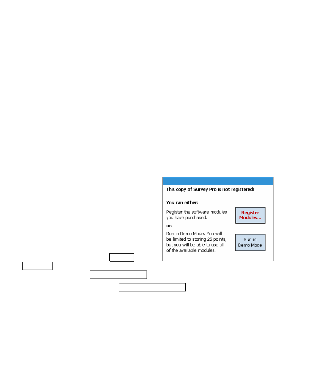
Registering

After Survey Pro is installed, the Standard Module must be registered for Survey Pro to be fully functional. If it is not registered, Survey Pro will only run in demo mode, which means all jobs will be limited to no more than 25 points, and if a job is stored on the data collector that exceeds this limit, it cannot be opened.

If you start Survey Pro and the standard module has not yet been registered, the screen

shown here will open. Tap the Register

Modules… button to access the Register Modules screen. To run in

demo mode, simply tap Run In Demo Mode . To register your Modules, tap the Enter Registration Code button.

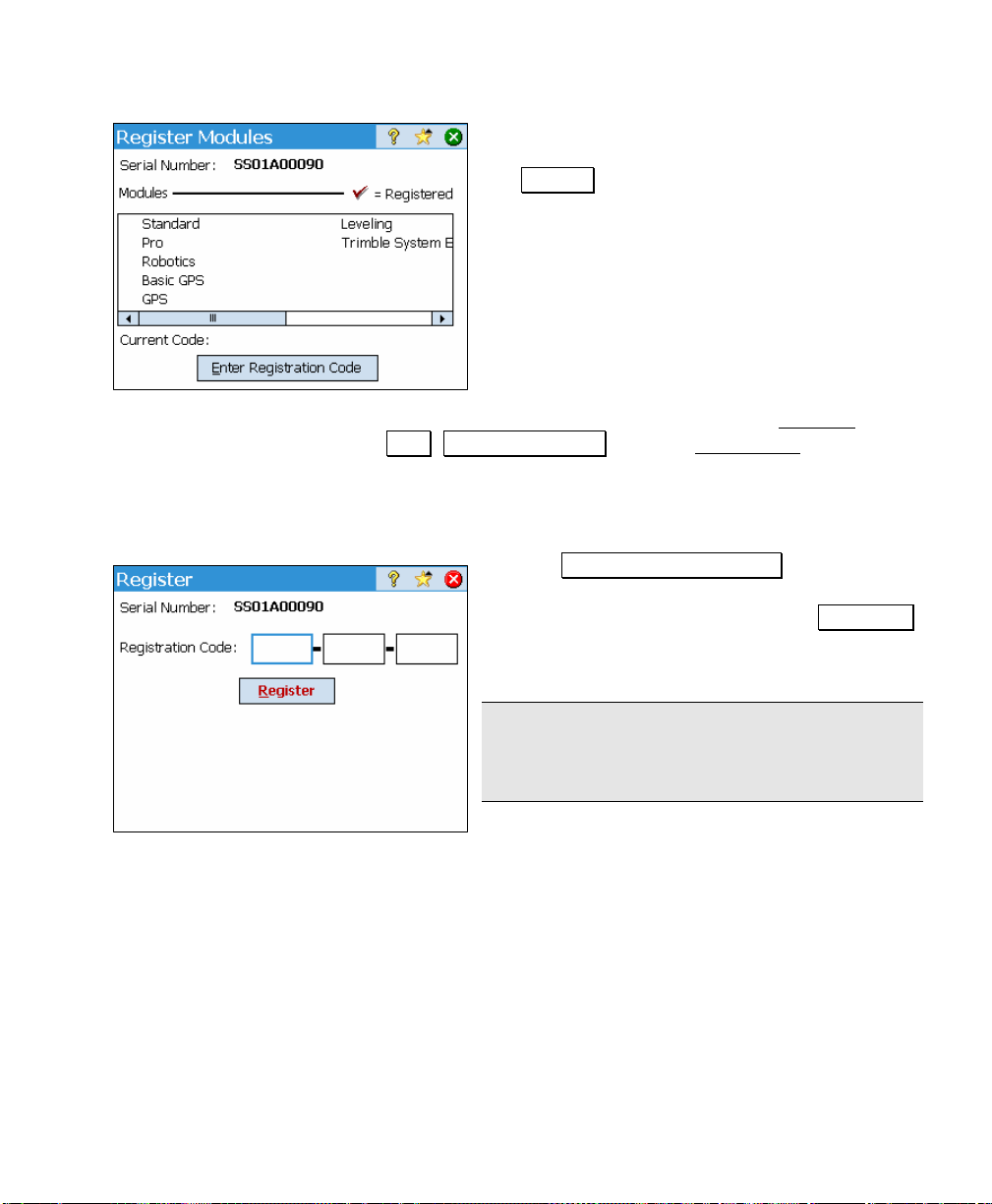
Getting Started

Enter the registration code provided by your TDS dealer in the Registration Code field and

tap Register. This will register all of the modules that you have purchased. If there are modules that you feel should be registered but are not, contact TDS tech support.

Add-on modules can also be purchased from your local TDS dealer to upgrade your TDS Survey Software. Upgrading involves simply registering the appropriate module using the same method as described above

If you want to register a particular module, access the Register by tapping File , Register Modules from the Main Menu

screen

Contact your TDS dealer and give him your unique serial number that is displayed on this screen. He will give you a registration code for the module that you purchased.

Tap the Enter Registration Code button for the appropriate module, enter the registration code in the dialog box that opens and tap Register… . All the features for the module that you purchased will now be available.

Note: You should keep a record of all registration codes purchased in case they need to be reentered at some point.

User’s Manual

Angle and Time Conventions

Throughout the software, the following conventions are followed when inputting or outputting angles and time:

Azimuths

Azimuths are entered in degree-minutes-seconds format and are represented as DD.MMSSsss, where:

• DD One or more digits representing the degrees.

• MM Two digits representing the minutes.

• SS Two digits representing the seconds.

• sss Zero or more digits representing the decimal fraction

part of the seconds. For example, 212.5800 would indicate 212 degrees, 58 minutes, 0 seconds.

Bearings

Bearings can be entered in either of the followin g formats:

• S32.5800W to indicate South 32 degrees, 58 minutes, 0 seconds West.

• 3 32.5800 to indicate 32 degrees, 58 minutes, 0 seconds in quadrant 3.

Time

When a field accepts a time for its input, the time is entered in hoursminutes-seconds format, which is represented as HH.MMSSsss where:

• HH One or more digits representing the hours.

• MM Two digits representing the minutes.

• SS Two digits representing the seconds.

• sss Zero or more digits representing the decimal fraction

part of the seconds.

Getting Started

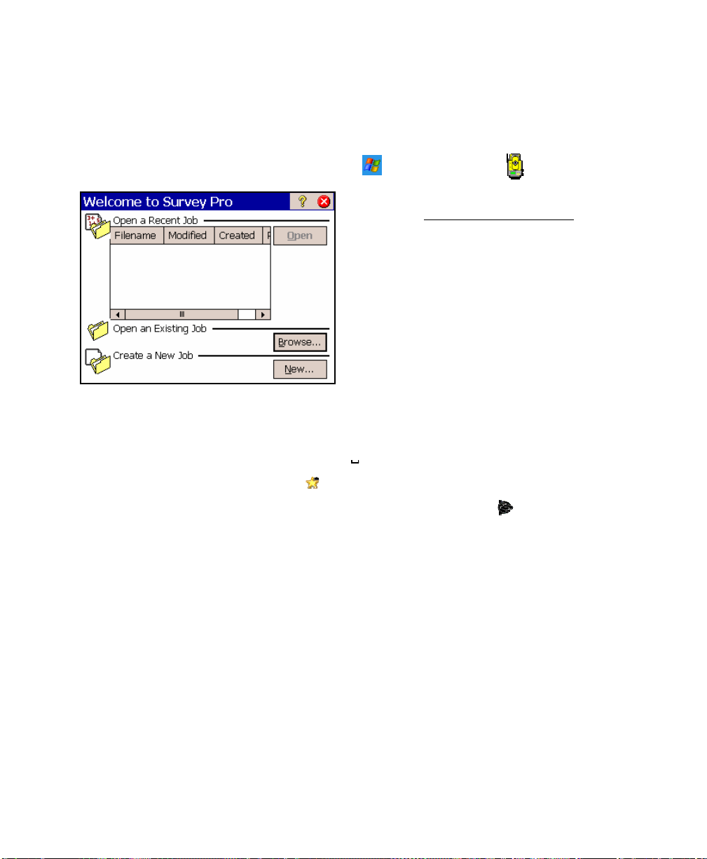
Using Survey Pro

To start Survey Pro, tap Start > Programs >

Survey Pro cannot start without a job being open so the Welcome to Survey Pro ask if you want to open a recently opened job, open an existing job, or create a new job. For this example we will create a new job so you can begin exploring the software.

Selections and cursor control in Survey Pro can be made by simply tapping the screen with your finger or a stylus.

You can temporarily disable the touch-screen if you need to clean it by using any of the methods below:

screen will

• Press [CTRL] - [

• Use the

• Ranger 300X/500X only: Press [Fn] - [

Repeat to reactivate the touch-screen.

] and press [ESC] to reactivate the screen.

, Suspend Screen quick pick.

] (Trimble logo).

User’s Manual

1. Tap the New… button. The Create a New Job dialog box will open, which prompts you for a job name where the current date is the default name.

2. Either type in a new job name or accept the default name. Control points can optionally be used or imported from another existing job by checking the Use or Import a Control File checkbox. (See Page 31 for more information on control files.) For this example, leave this unchecked and tap

Next > to continue.

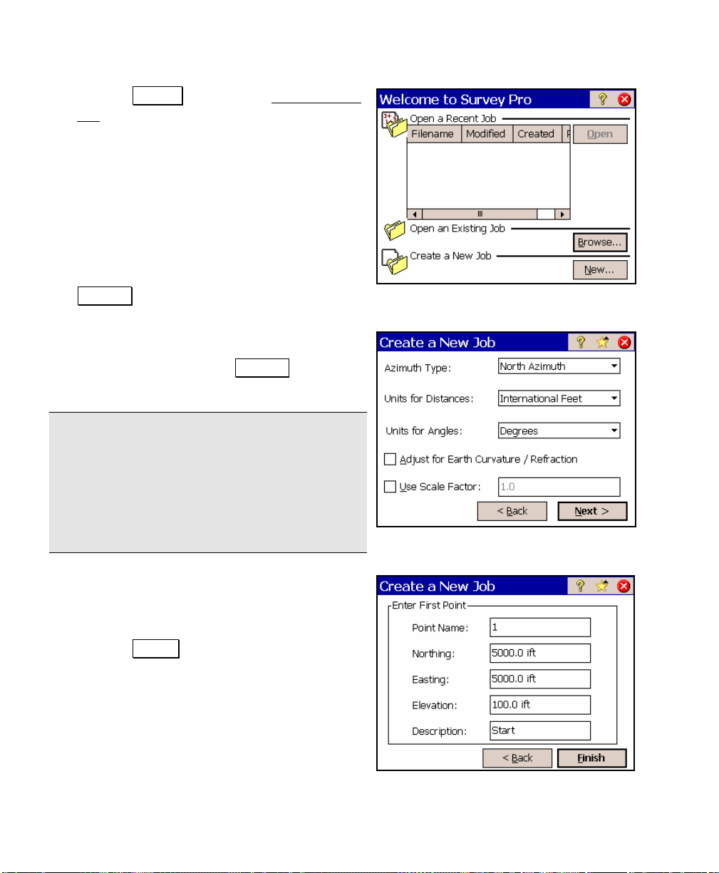
Another screen will open where you select some of the job settings. Select the settings

that you desire and tap Next > to continue.

Note: When creating a new job, it is important that the Units for Distances field be set to the correct units. This allows you to seamlessly switch between different units in mid-job. Problems can arise if these units are inadvertently set to the incorrect units when new data is collected.

3. Since all jobs must have at least one point to start with, the final screen displays the default point name and coordinates for the first point. Accept the default values by

tapping Finish . This will create and store the new job. You are now ready to explore the software.

Getting Started

Note: The settings and values entered for a new job become th e default values for any subsequent new jobs with the exception of the Use Scale Factor setting, which always defaults to off.

Navigating Within the Program

The starting point in Survey Pro, which appears once a job is open, is called the Main Menu, shown here. All the screens that are available in Survey Pro are accessed startin g from the Main Menu screens in Survey Pro will eventually take you back to the Main Menu

. Likewise, closing the

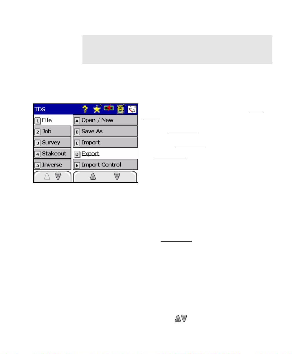
The Main Menu left column contains all of the available menus and the column on the right contains the menu items associated with the active menu.

When a menu is selected from the left column, th e corresponding menu items will become available in the right hand column. When a menu item is activated from the right hand column, the corresponding screen will open. It is from these screen s where you do your work.

Navigation through the menus and menu items can be done using any of the methods described below. The best way to become familiar with navigating through the Main Menu

Each menu has a number associated with it, whereas the menu items have letters associated with them. Pressing the associated number or letter on the data collector’s keypad will activate th e corresponding menu or menu item.

You can scroll through the list of menus and menu items by using the arrow keys on the keypad. The up and down arrow keys will scroll up and down through the selected column. The other column can be selected by using the horizontal arrow keys.

You can also scroll through the list of menus and menu items by tapping the special arrow buttons

consists of two columns. The

is to simply try each method.

on the screen located at the

User’s Manual

bottom of each column. If one of these buttons appears blank, it indicates that you can scroll no further in that direction.

When the desired menu item is selected, it can be activated by tapping it or pressing the [Enter] key on the keypad.

Command Bar

The command bar is the top portion of each Survey Pro screen and it contains buttons that are appropriate for the current screen. All of the possible buttons are described below.

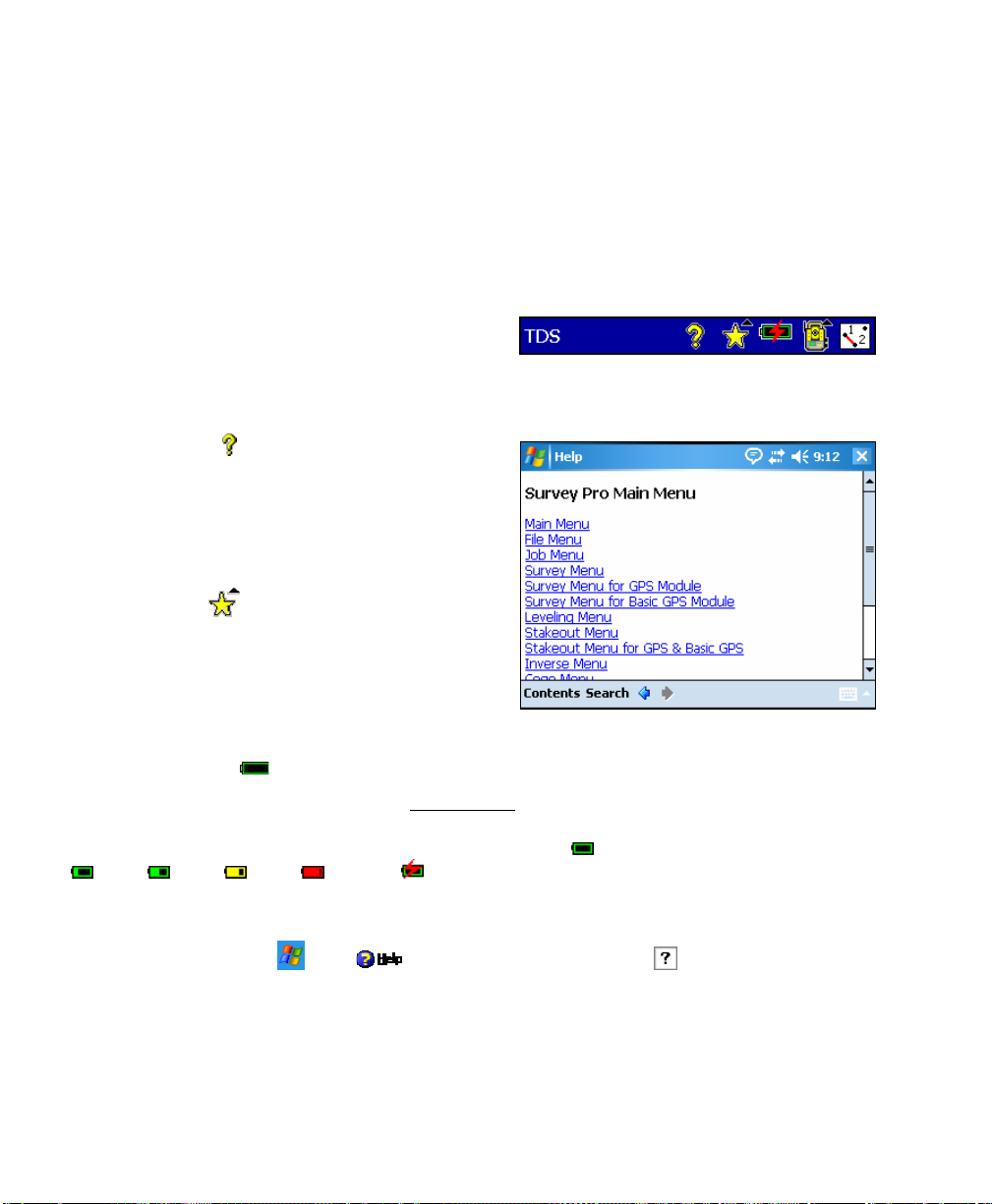
Online Help

This button opens the online help, which allows you to access information for each screen similar to the information you would find in the reference manual.

Quick Pick

The Quick Pick button will open a customizable list of routines. To quickly access a routine, just tap on it. See Page 18 for more information.

Battery Level

The battery icon at the bottom of the Main Menu displays the condition of the Survey Pro’s rechargeable batt ery. T he icon has five variations depending on the level of charge remaining:

75%, 50%, 25%, 5% and charging.

Tapping the battery icon is a shortcut to the Microsoft Power Settings screen. You can view the online help for this screen on a Rang er

300X/500X by tapping

then

, or on a Ranger by tapping .

100%,

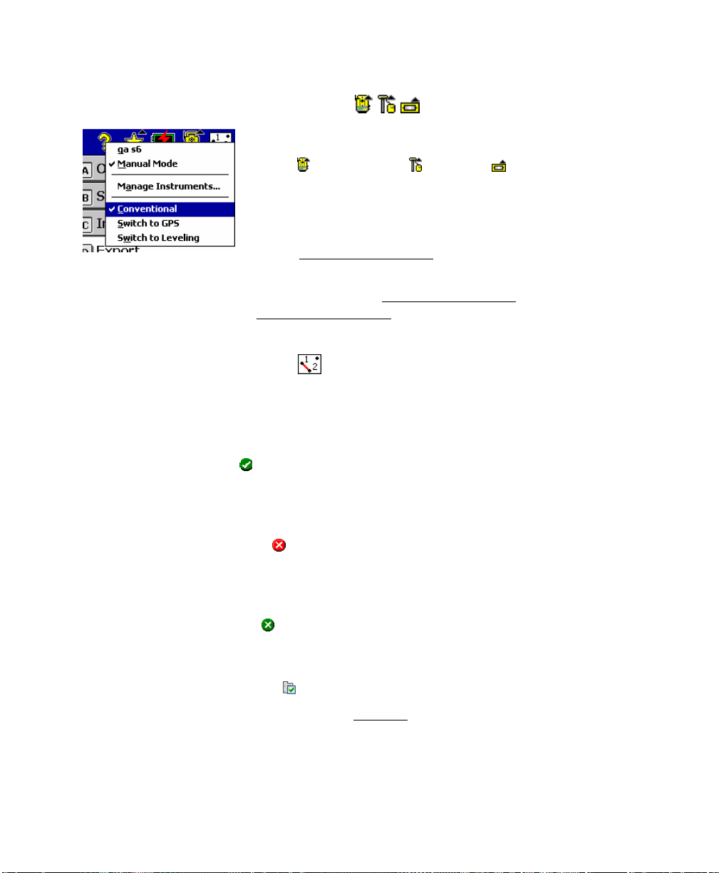
Surveying Mode

The instrument icon indicates which collection mode the software is running in. There are three possible surveying modes: icon will open a list of options to do any of the f ol lowing:

for more information.)

Conventional, GPS, and Leveling. Tapping this

• Switch to another instrument mode.

• Quickly select a different instrument profile. (See the

Instrument Settings

screen in the Reference Manual

Getting Started

• Quickly access the Instrument Settings Instrument Settings information.)

screen in the Reference Manual for more

screen. (See the

Map View

This button will access the map view of the current job when it is tapped. The map view is available from m any screens and is discussed in detail on Page 22.

This button performs the desired action then closes the current screen.

Cancel

This button is red in color and closes the current screen without performing the action intended by the screen.

This button is green in color and closes the current screen.

Settings

This button opens the Settings screen associated with the curre nt screen.

User’s Manual

GPS Status

This is used to view the current status and access the settings for a GPS receiver when using the GeoLock feature (Page 135). This is only available from the Remote Control using a supported robotic total station.

and Remote Shot screens when

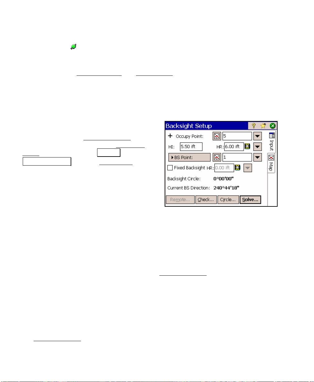
Parts of a Screen

Many screens share common features. To illustrate some of these features, we will examine parts of the Backsight Setup shown here. You can access the Backsight

Setup screen by selecting .Survey ,

Backsight Setup from the Main Menu.

screen,

Input Fields

An input field is an area where a specific value is entered by the user. An input field consists of a point label, which identifies the data that is to be entered in that field. It has a rectangular area with a white background, where the data is entered. A field must first be selected before data can be entered in it. You can select a field by tapping on it or pressing the [Tab] key on the data collector repeatedly until it is selected. When a field is selected, a dark border is drawn around it and a blinking cursor is inside the field. In the Backsight Setup screen above, the Occupy Point field is selected.

Output Fields

Output fields only display information. These fields typically display values in bold text, do not have a special colored background, and the value cannot be changed from the current screen. For example, in the Backsight Setup field.

screen, the Backsight Circle value is an output

Getting Started

Power Buttons

The Backsight Setup screen contains two power buttons. Power buttons are typically used to provide alternate methods of entering or modifying data in the corresponding field. To use a pow er but t on, simply tap it. Once tapped, a dropdown list will appear with several choices. The choices available vary depending on with which field the power button is associated with. Simply tap the desired choice from the dropdown list.

Tapping the first power button in the Backsight Setup screen allows you to specify an occupy point using other methods or view the details of the currently selected point. You should experiment with the options available with various power buttons to become familiar with them.

Choose From Map Button

The Choose From Map Button is always associated with a field where an existing point is required. When the button is tapped, a map view is displayed. To select a point for the required field, just tap it from the map.

Note: If you tap a point from the map view that is located next to other points, another screen will open that displays all of the points in the area that was tapped. Tap the desired point from the list to select it.

Scroll Buttons

When a button label is preceded with thesymbol, it indicates that the button label can be changed by tapping it, thus changing the type of value that would be entered in the associated field. As you continue tapping a scroll button, the label will cycle through all the available choices.

In the Backsight Setup point or a direction by toggling the scroll button between

BS Point and BS Direction .

Button.

screen, the backsight can be defined by a

User’s Manual

Index Cards

Many screens actually consist of multiple screens. The different screens are selected by tapping on various tabs, which look like the tabs on index cards. The tabs can appear along the top of the screen or the right edge.

The Backsight Setup and the other is titled Map.

The Settings accessing several screens and is discussed in more detail starting on Page 27.

screen has a variant of the Index Card format for

screen consists of two cards. One is titled Input,

Input Shortcuts

Distances and angles are normally entered in the appropriate fields simply by typing the value from the keypad, but you can use shortcuts to simplify the entry of a distance or angle.

If you want to enter the distance between two points in a particular field, but you do not know offhand what that distance is, you can enter the two point names that define that distance separated by a hyphen. For example, entering 1-2 in a distance field would compute the horizontal distance from Point 1 to Point 2. As soon as the cursor is moved from that field, the horizontal distance between the points will be computed and entered in that field.

An alternate method to using this shortcut is to tap the button, select Choose from map… and then tap the two points that define the distance that you want to enter. Once you tap Map View appear in the corresponding field.

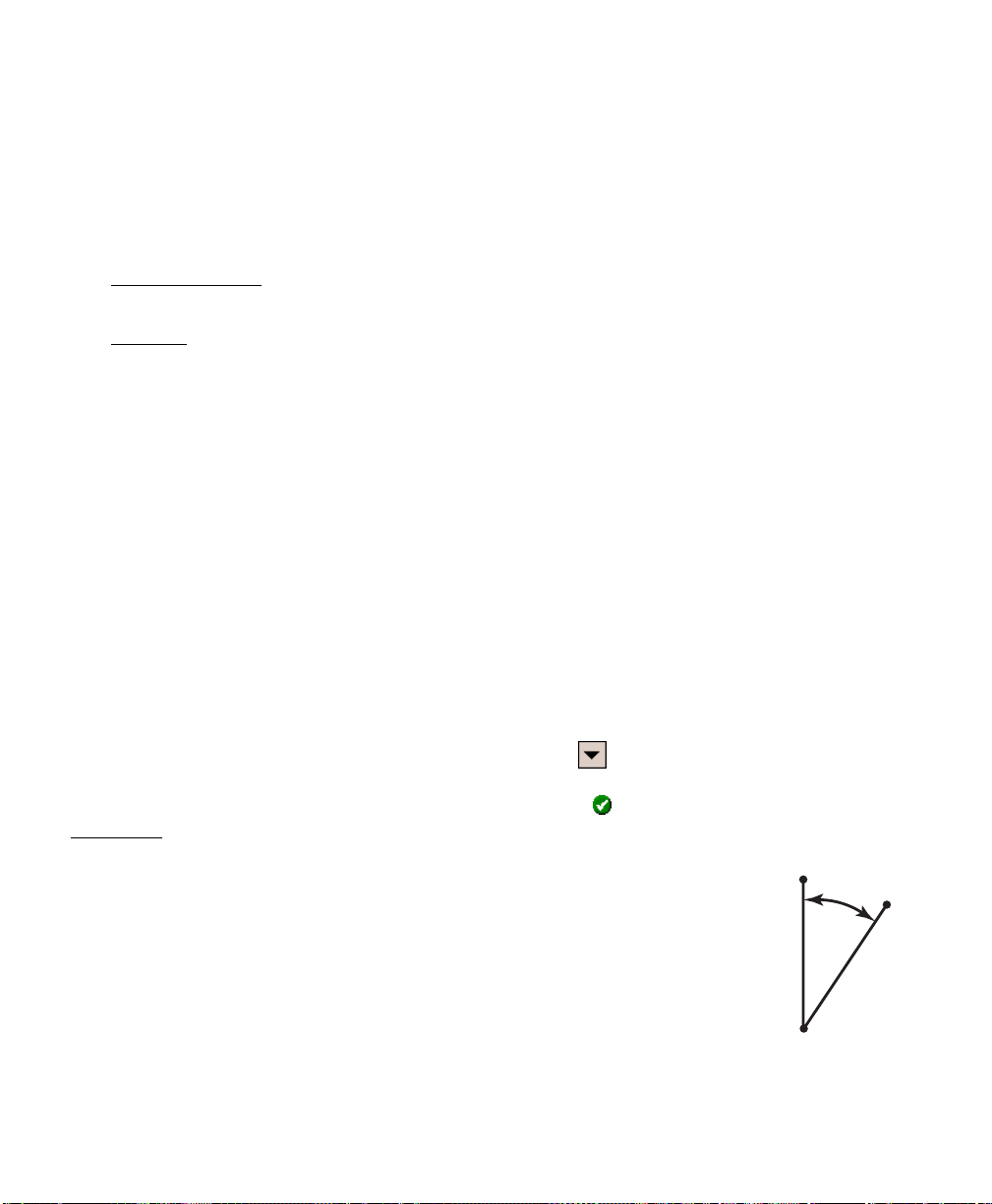
Likewise, there is a similar shortcut to enter angles in fields that accept them. If you wanted to enter the angle, α, from the illustration shown here, you would simply enter 1-2-3 in the appropriate field. As soon as the cursor is moved from that field, the angle formed by the three points entered will be entered in that field. As with specifying a distance, you could also use the power button as described above and tap the points of the angle in the correct order.

, the horizontal distance between the two tapped points will

power

from the

Another shortcut can be used to enter distances with fractional inches (architectural units). Simply key in the feet, inches, and fractional

Getting Started

inches where each value is separated by a space and the fraction is entered using a forward slash (/). For example, to enter 3 feet, 6 and 3/32 inches, you would key in 3 6 3/32. Once the cursor leaves that field, the distance will automatically be con verted to the appropriate decimal distance.

If working with distances under 1 foot, it is acceptable to exclude the feet value; for example "8 5/64" would be interpreted as 8 and 5/64 inches. Likewise, if entering a fractional distance under an inch, you would only enter the fractional inch.

The following details should be considere d when using the above method to enter fractional inches:

1. When the job is configured for International Feet or US Surve y Feet, it is assumed that the distance entered is in the same units as the job is configured for.

2. If the job is configured for meters, it is assumed that the distances entered are in International Feet and will be converted to meters when the cursor leaves the current field. (You cannot use this method to enter a metric distance in fractional format.)

3. If a fractional inch is entered that cannot be evenly divided by 1/64 inch, it will automatically be converted to the nearest 64

inch. This conversion would be negligible for survey data and unlikely to occur.

An alternate method to using this shortcut is to tap the

Quick Pick button while the cursor is in a distance field that you want to change and select AU Conversion. Enter the appropriate feet, inches and

fractional inches and tap Use . See the Reference manual for more information on the AU Conversion screen.

User’s Manual

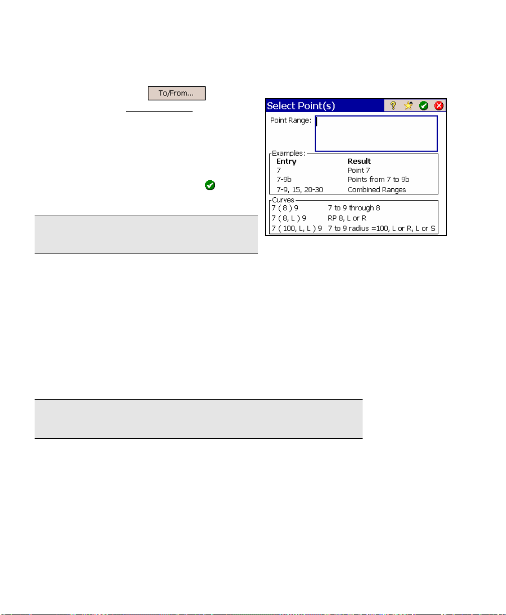
Point List Editor

Many screens contain a button, which accesses the Select Point(s) allows you to enter a simple list of points or a list of points that describe a line that can contain curves.

Examples of how to enter different lists of points are displayed in the lower portion of the screen. Once the list is entered, tap return to the previous screen.

Note: Spaces in point lists are ignored. They are only used in the examples for clarity.

The examples for entering the three possible curve types are explained in detail as follows:

• 7 ( 8 ) 9

The first example, defines a curve that passes through Points 7, 8 and 9, respectively.

screen that

• 7 ( 8, L ) 9 The second example defines a curve where Point 8 is the radius point and the curve begins to the Left (from the point of view of the radius point), turning from Point 7 to Point 9.

Note: When defining a curve with a radius point, the other two points must be the same distance from the radius point for a solution.

• 7 ( 100, L, L ) 9 The third example describes a curve with a radius of 100, using the same units as the job, that begins at Point 7, turning to the Left (from the point of view of the radius point), creating a Large arc (> 180°), and ending at Point 9.

Getting Started

Entering Distances in Other Units

When a distance is entered in a particular field, it is normally entered using the same units that are configured for the current job, but distances can also be entered that are expressed in other distance units.

When entering a distance that is expressed in units that do not match those configured for the job, you simply append the entered distance with the abbreviation for the type of units entered. For example, if the distance units for your current job were set to International Feet and you wanted to enter a distance in meters, you would simply append the distance value with an m or M for meters. As soon as the cursor is moved to another field, the meters that were entered will be converted to feet.

The abbreviations can be entered in lower case or upper case characters. They can also be entered directly after the distance value, or separated with a space. The following abbreviations can be appended to an entered distance:

• International Feet: f or ft or ift

• US Survey Feet: usf or usft

• Inches: i or in

• Meters: m

• Centimeters: cm

• Millimeters: mm

• Chains: c or ch

User’s Manual

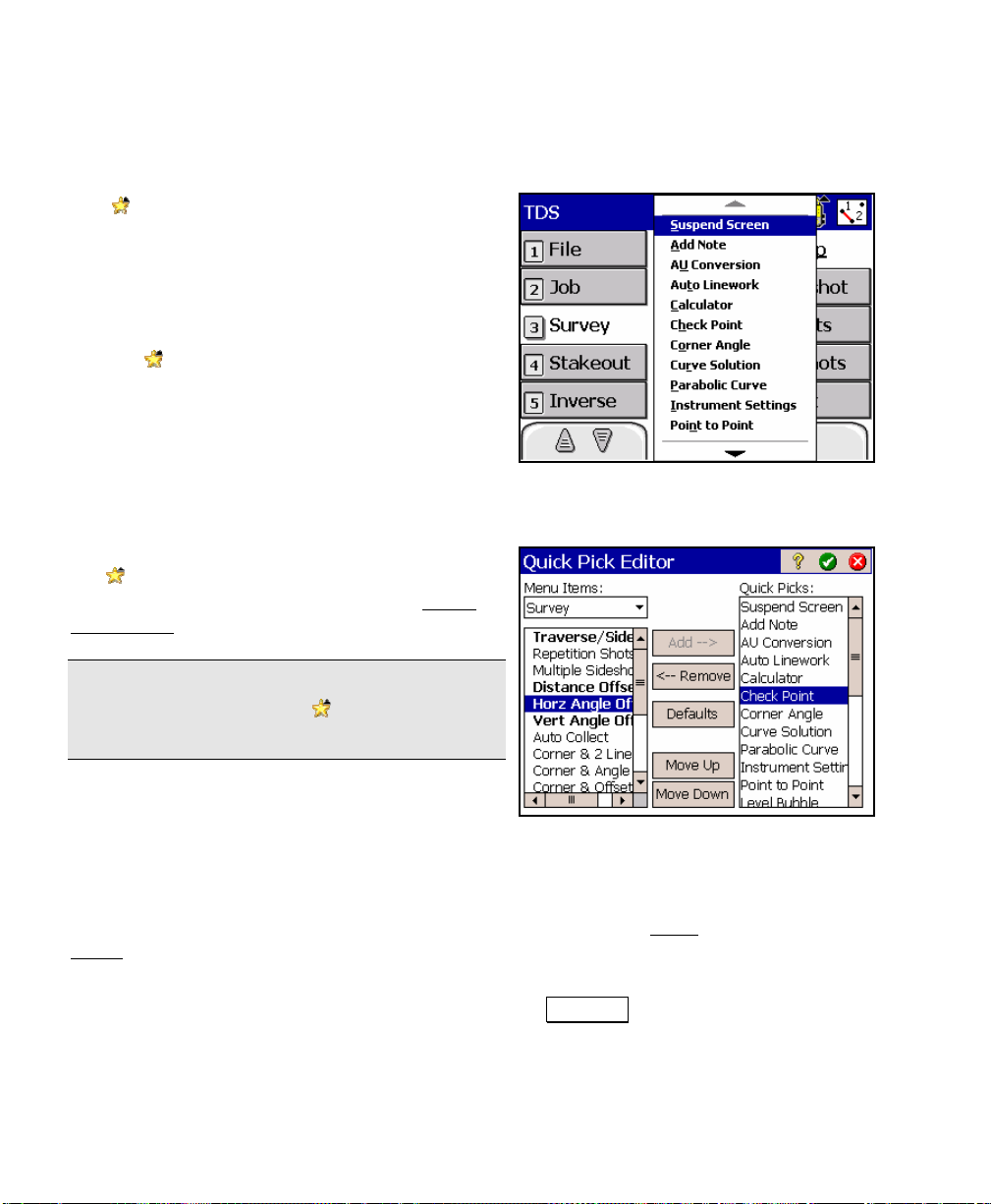
Quick Pick

The button is called the Quick Pick button. This button is used to quickly access any of several commonly-used routines. The list of routines available from the Quick Pick button can be customized and sorted in any order.

To access a screen with the Quick Pick button, first tap

Customizing the Quick Pick List

If you want to customize the Quick Pick list, tap and tap Edit Quick Pick. This opens the Quick Pick Editor.

and then tap the desired routine.

and then scroll to the bottom of the list

Tip: You can quickly get to the bottom of the Quick Pick list by tapping then pressing the up-arrow hardware button once.

The current Quick Pick list is displayed in the right column and the routines that can be added to the list are displayed in the left column, where the routines that are already in the Quick Pick list are shown in bold.

To add a routine, first select the menu item from the Menu Item dropdown list where that routine is normally accessed from the Main Menu. (Not all routines can be added to the Quick Pick list. If a routine is not listed, it cannot be added.)

Select the routine from the left column then tap th e Add --> button to add it to the Quick Pick list on the right.

Getting Started

The new routine will initially be placed at the bottom of the list. To move it elsewhere in the list, select it and tap the Move Up or

Move Down buttons. (Any other routines in the Quick Pick list can

also be repositioned in this way.) To remove a routine from the Quick Pick list, select it and tap the

<-- Remove button.

Tapping the Defaults button will revert the custom list back to the default list. Since any changes will be lost, a prompt will first ask if you are sure.

Smart Targets

Survey Pro has the ability to create and store custom configurations for any number of prisms or other target types. These are called Smart Targets.

Smart Targets are useful when working with multiple prisms on the same job, particularly when the prisms have different characteristics such as rod height and/or offset because the user can quickly switch between different Smart Targets before taking a shot.

Smart Targets also provide a way to quickly switch between taking a shot at a prism and taking a shot at a reflectorless target. The total station EDM configuration is switched for you automatically.

Selecting Smart Targets

You can quickly select any existing Smart Target from a screen that has an HR field. Tap the power button HR field that you want to shoot. A

power button indicates a prism target type is currently selected. A icon indicates a reflectorless target type is currently selected

All the available Smart Targets will be displayed in the upper portion of the drop-down list. The Smart Targets listed will depend on if you are selecting a Smart Target for your foresight or your backsight.

Simply tap the Smart Target that you want to use from the drop-

corresponding with the

icon displayed next to the

User’s Manual

down list. The preset configuration for the selec ted Smart Target will be automatically set.

Manage Smart Targets

Select Manage Smart Targets from the same drop-down list described above to access the Manage Smart Targets can create a new custom Smart Target or edit any existing Smart Target.

Survey Pro includes two foresight Smart Targets called My Prism and My Reflectorless, respectively and one backsight Smart Target called My Backsight Prism. These can be edited or deleted, but at least one prism and one reflectorless foresight Smart Target and at least one prism backsight Smart Target must exist at all times. Because of this, for example, you would not be able to delete My Backsight Prism unless another Smart Target with a prism target type for your backsight was available. Similarly, you would not be able to change My Reflectorless to a prism target type unless you already had another foresight Smart Target configured with a reflectorless target type.

screen. From here you

To delete an existing Smart Target, tap it to select it and then tap

Delete .

Tapping Sort will sort the list of Smart Targets alphabetically. You can also activate a Smart Target from this screen by tapping the

desired Smart Target to select it and then tapping Activate , although it’s faster to activate Smart Targets using the shortcut described above. The active Smart Target is shown with a next to it.

symbol

Getting Started

To create a new Smart Target tap the Add… button. To edit an existing target, tap it from the list to select it and then tap Edit… . Either option will open the Edit Smart Target screen.

The Smart Target Name you provide will be shown in the drop-down list when you switch between Smart Targets.

The Target Type field determines how the EDM will be configured on the total station when taking shots to the Smart Target. It can be

Prism when using a standard prism, Reflectorless to perform distance measurements without a prism, Long Range Prism, which increases the output power of the EDM for

shooting prisms at long distances, or On Gun, which uses the EDM settings configured on the total station (Leic a only). Not all target types are supported by all total station.

Note: If using a Trimble S6/VX, there are special smart targ et settings available, which are described under Smart Targets in the Reference Manual.

The HR field will be the default rod height whene ver this Smart Target is selected. Updating the HR from any screen that has an editable HR field while a Smart Target is selected will also save that new value here, making it the new default HR for the current Smart Target.

If the Add Offset to HR is checked, the offset entered in the corresponding field will then be added to the rod height you provide. (A negative value would subtract the offset from the HR.) This is useful for people who use a device that always elevates their rod by a fixed distance, but still want to use the rod height measurement displayed on the rod for simplicity.

For example, if you were in the Backsight Setup

screen and selected a foresight Smart Target with a default HR of 5 feet and an HR offset value of 1 foot, you would see 5.00 ift displayed in the foresight HR field of the Backsight Setup

screen, as well as every other editable

foresight HR field, but you would see 5.0+1.0 ift in every output -only

User’s Manual

HR field showing the HR entered plus the offset. (The raw data file will also clearly note when a rod height offset is being applied.)

The Prism Constant field should contain the prism constant for the prism associated with this Smart Target as long as a prism constant is not also set in the total station. If a prism constant is set in Survey Pro and on the total station, it will be applied twice resulting in incorrect distance measurements for every shot.

If you are using a robotic total station that supports prisms that output a target ID, the Use Target ID field will be available where you can specify the target ID for the Smart Target.

If Use For Search is available and selected, the total station will only look for the Target ID when it is searching for the targ et. Once the target is found, it will track the prism, but it is possible for the total station to start tracking a different reflector that comes into view. If Use Always is selected, the total station will continuously monitor the Target ID and only track the prism with the specified Target ID.

Tap

to close the Edit Smart Targets screen and save any changes.

Map View

from the command bar, or from various screens

Many screens provide access to a map view. The map view is a graphical representation of the objects in the current job.

Map View without basemaps Map View with basemaps

Getting Started

There are different map views depending on from where the map view is accessed and they can display slightly different information such as a vertical profile.

The main map view is accessed from the Main Menu by tapping the

button at the bottom of the screen in the command bar. If you are using basemaps, it is from this map view where the basemaps are managed.

All other map views are accessed by tapping the

button from a

variety of screens. A bar is shown at the bottom of every map view that indicates the

scale. The buttons along the left edge of the screen allo w you to change

what is displayed in the map view.

Tip: You can pan around your map by dragging your stylus across the screen.

Zoom Extents Button: will change the scale of the screen so that

all the points in the current job will fit on the screen.

Zoom In Button: will zoom the current screen in by

approximately 25%.

Zoom Out Button: will zoom the current screen out by

approximately 25%.

Zoom Window Button: Allows you to drag a box across the screen. When your finger or stylus leaves the screen, the map wil l zoom to the box that was drawn.

Zoom To Point Button: Prompts you for a point name and then the map view will be centered to the specified point with the point label displayed in red.

Turn To Point Button: Tap this button and then tap a point in the map view to automatically turn the total station to the selected point. This is only available when a robotic total station is selected and Remote Control is active in the Instrument Settings

User’s Manual

Increase Vertical Scale: is only available when viewing a vertical profile. Each time it is tapped, the vert ical scale of the view is increased.

Decrease Vertical Scale: is only available when viewing a vertical profile. Each time it is tapped, the vert ical scale of the view is decreased.

Zoom Preview Button: will display only the points that are currently in use (only available from certain map view screens).

Map Display Options: Accesses the Map Display Options screen, described below.

Manage Basemaps: Accesses the Manage Basemaps screen, described below (only available from the main map view, access ed from the command bar button in Main Menu).

Basemaps

Basemaps can be used in jobs to more accurately display local objects and terrain in the map view to give the surveyor a better idea of where they are in relation to local land features.

There are two general types of basemaps – raster images and CAD drawings. Raster images are usually created from photographs and can accurately display the local terrain with great detail. CAD drawings are created from CAD software and will typic ally display points, roads, boundaries and any other objects that can be drawn with lines.

Basemap Files

Survey Pro supports basemap files from AutoCAD, GeoTiff, and TDS. Since basemap files can be large in size, the following points should

be considered when managing basemap files:

Getting Started

• Before you can use a basemap in Survey Pro, you need to copy the appropriate basemap files from a PC to the same directory where your current job is located. If the basemap files are stored in a different directory and then added to the current job, the files will be copied to the job’s directory.

• If you use the Save As routine and save the current job to a new directory, any basemaps associated with that job will be copied to the new location.

Manage Basemaps

Once the basemap files are stored on the data collec tor, they must be added to the current job before they can be viewed in the map view.

1. To add basemaps, open the Main Map View by tapping the button in the command bar from the Main Menu.

2. From the main Map View button to open the Manage Basemaps screen shown here.

3. Tap the Add… button. This will open a new screen where you can select the basemap that you want to add to the current job.

4. Once a basemap is added, it will appear in the list in the Manage Basemaps

5. Repeat Steps 3 and 4 to add any additional basemaps.

, tap the

screen.

User’s Manual

Basemaps are drawn to the screen in the reverse order that they are listed in the Manage Basemaps

screen, where the first basemap in the list is the last one drawn, and thus, will be drawn "on top" of any other basemaps. This is important to remember if any basemaps overlap since if a raster basemap were drawn on top of another basemap, it would cover any basemaps below it.

The list shown contains a vector basemap, tds.dxf that occupies the same area as the other two basemaps, which are raster basemaps. The vector basemap is at the top of the list so the points and lines it contains will be drawn last and appear on top of the two raster basemaps.

6. To change the order of the basemaps in

the list, select a basemap and tap the

Move Up or Move Down buttons to move it up or down in the list, respectively.

7. To remove any basemap from the list, select it and tap Remove . This will remove the basemap from the list and

un-associate it from the current job. (This will not delete the corresponding basemap file.)

Raster basemap drawn first.

Vector basemap drawn last.

Resulting map view with both basemaps in view.

Getting Started

8. The colors of the objects in vector basemaps can be modified by selecting the basemap

and then tapping Edit… to open the Edit Basemap screen.

The Settings Screen

The Settings screen is used to control all of the settings available for your total station, data collector, current job, and Survey Pro software.

Most of the settings remain unchanged unless you deliberately change them, meaning the default settings are whatever they were set to last. For example, if you create a new job where you change the direction units from azimuths to bearings and then create another new job, the default direction units for the new job will be bearings.

Survey Pro behaves in this way since most people use the same settings for a majority of their jobs. This way, once the settings are set, they become the default settings for all new jobs and current jobs.

Some settings are considered critical and are therefore stored within the job. The following settings are stored within a job and will override the corresponding settings in the Settings opened:

• Scale Factor – Surveying Settings Card

• Earth Curvature On or Off – Surveying Settings Card

• Units for Survey Data (distances) – Units Settings Card

• North or South Azimuth – Units Settings Card

• Angle Units – Units Settings Card

screen when it is

User’s Manual

• GPS setup information such as localization, mapping plane, etc. (Requires GPS Module)

The Settings independent screens where each individual screen contains different types of settings. There are two ways to navigate to the various screens. The first method is to tap the button to drop down the list of available screens and then tap on the desired screen from the list to open it. The second method is to tap the buttons to the side of the screen title, which will open the previous or next screen respectively. For example in the screen shown, you could tap (General Settings Settings) screen. Repeatedly tapping either of these buttons will cycle through all the available screens.

Consult the Reference Manual for an explanation of each field on every Settings

If using a Bluetooth total station, refer to the Bluetooth section on Page 294.

screen actually consists of several

to open the previous

) screen, or tap to open the next (Units

screen.

File Management and ForeSight DXM

Survey Pro uses a variety of files to store data and inform ation about your project. The files include t h e main data file, the .JOB file, and the raw data file, the .RAW file, and several other supplementary files that Survey Pro can use for additional information. To help manage this data and to supplement Survey Pro capabilities, TDS has an office product called ForeSight DXM.

ForeSight DXM is a complete data management tool that works directly with Survey Pro data files. ForeSight DXM can make any project easier to manage and makes doing every day tasks, such as downloading, quick and easy. ForeSight DXM has a variety of

Getting Started

analysis tools, geodetic tools including projection setups, and the capability to convert TDS data files into many other formats, including LandXML, for use in CAD.

ForeSight DXM makes the field-to-office and the office-to-field process seamless and easy. If you don’t already own a copy of ForeSight DXM, contact your TDS Dealer for more information. You can also download a full-featured demonstration copy of ForeSight DXM from the TDS Web site at www.tdsway.com

Job Files

Every job that is used with TDS Survey Pro actually consists of at least two separate files; a job file and a raw data file. Each file performs a different role within the software.

A job file can be created in the Data collector, or on a PC using TDS ForeSight DXM (or other PC software) and then transferred to the Data collector. It is a binary file that has a file name that is the same as the job name, followed by a *.JOB extension. A job file is similar to the older TDS-format coordinate file, except in addition t o stori ng point names and their associated coordinates, a job file also contains all of the line work as well.

When you specify points to use for any reason within Survey Pro, the software will read the coordinates for the spec ified points from the job file. Whenever you store a new point within Surv ey Pro, the point is added to this file.

A job file can be edited on the Survey Pro when using the Edit Points screen. Since a job file is binary, it requires special soft ware for editing on a PC, such as TDS Survey Link. It can also be converted to or from an ASCII file using Survey Link. (Refer to the Surve y L ink documentation for this procedure.)

When a job file is converted to an ASCII file, the resulting file is simply a list of points and coordinates. Each line consists of a point name, northing or latitude, easting or longitude, elevation or elliptical height, and a note where each value is separated by a comma.

User’s Manual

Raw Data Files

A raw data file is an ASCII text file that is automatically generated whenever a new job is created on Survey Pro and cannot be created using any other method. It has the same file name as the current job file (the job name), followed by the *.RAW extension.

A raw data file is essentially a log of everythin g that occurred in the field. All activity that can create or modify a point is written to a raw data file. Survey Pro never "reads" from the raw data file – it only writes to the file. Since a raw data file stores all of the activity that takes place in the field, it can be used to regenerate the original job file if the job file was somehow lost. This process requires the TDS Survey Link software.

Since a raw data file is considered a legal document, it cannot be edited using any TDS software other than appending a note to it using the View Raw Data invalidate all of its contents and is not supported in any way by TDS.

When viewing a raw data file on a PC using a simple text editor or on Survey Pro using the View Raw Data unaltered, which can appear somewhat cryptic. When viewin g the file from within Survey Link, the codes are automatically translated on the screen to a format that is easier to understand.

screen. Editing a raw data file would

screen, the file is shown

Getting Started

Control Files

The current job can be configured to access the points from another job stored on the data collector. When the current job is using p oints from another job, that other job is called a Control File and the points in the control file are called Control Points. (Any non-point objects in a control file are always ignored.)

A control file can be selected from the New Job wizard when creating a new job, or the File Import Control screen can be used to select a control file for an existing job, or to manage the current control file.

See the Reference Manual for more information on these screens. There are two methods for accessing control points: imported control

points and external control points. Each method has advantages and disadvantages, which are explained below.

Import Control File

When a control file is imported, the control points are copied into the current job and stored on a special layer called CONTROL.

Importing control points provides improved RAW data consistency since each control point is written to the raw data file as a store point. This can significantly help when regenerating points from RAW data and generating reports in the office.

Importing control points may not be the best method when using very large control files, while collecting relatively small sets of points since the imported control points can make the current job very large with too many points to easily manage.

Importing control points is also not recommended when you want to switch between different control files from the curren t j ob.

User’s Manual

External Control File

When using an external control file, the points in the control fi le are simply linked to the current job and do not become a permanent part of the current job. Because of this, an external control file can later be unlinked, or cleared from the current job.

Some users prefer to keep a set of known points in a separate c ontrol file when repeatedly working on new jobs in the same general area. That way when they return to the job site, they can create a new job, but select the external control file to easily have access to the known control points.

Once an external control file is selected, the control points can be used in the same way as the job’s points with the following exceptions:

• An external control file has read only attributes. This means that the points in the control file cannot be modified or deleted; they can only be read. For example, you can select a control point to use as an occupy point during data collection or as a design point during stake out, but you could not use a control point for a foresight where you intend to overwrite the existing coordinates with new coordinates. You would a lso be unable to modify a control point from the Edit Points

screen.

• Since the points in an external control file are shar ed with the points in the current job, you cannot open an external control file if any of the point names used in it are also used in the current job. If you attempt to do so, a dialog will tell you that a duplicate point name was encountered and the control file will not be opened.

Getting Started

Description Files

A Description File is used to automate the task of entering descriptions for points that are stored in a job. They are especially useful when the same descriptions are frequently used in the same job.

A description file is a text file containing a list of the descriptions that you will want to use with a particular job. The file itself is usually created on a PC, using any ASCII text editor such as Notepad, which is included with Microsoft Windows. It is then saved using any file name and the .txt extension and then transferred to the Data Collector.

It is important to realize that when you use a more sophisticated application, such as a word processor to create a description file, you must be careful how the file is saved. By default, a word processor will store additional non-ASCII data in a file making it incompatible as a description file. However this can be avoided if you use the File > Save As… routine from your word processor and choose a Text Only format as the type of document to save. For more information on creating a text file using a word processor, refer to your word processor’s documentation.

Description files can be created in two different formats; one includes codes and the other does not. The chosen format determines how descriptions are entered. Each format is described below.

Description Files without Codes

A description file that does not contain codes is simply a list of the descriptions that you will want to use in a job. The content of a sample description file, without codes, is shown here.

The following rules apply to description files without codes:

• Each line in the file contains a separate description.

• A description can be up to 16 characters in length (including

spaces).

User’s Manual

• A description can contain any characters included on a keyboard.

• Descriptions do not need to be arranged in alphabetical order. (Survey Pro does that for you.)

• Descriptions are not case sensitive.

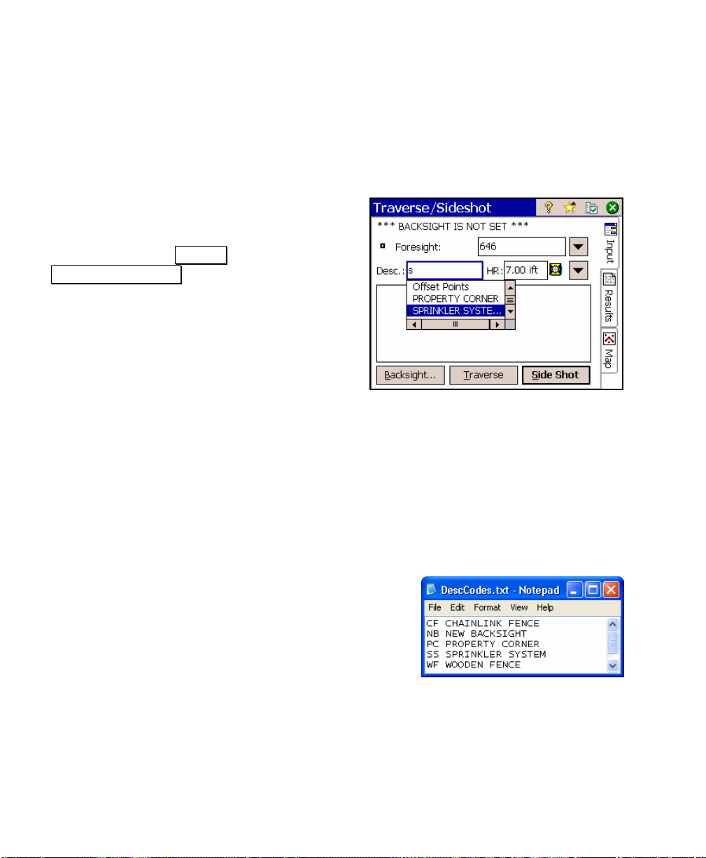
To use a description from a description file, simply start typing that description in any Description field. (You can experiment with

descriptions in the .Survey ,

Traverse / Sideshot screen.) Once you start typing a description, a dropdown list will appear displaying all of the descriptions in the descriptor file along with all the descriptors that have been used in the current job in alphabetical order. If the first letter(s) that you typed match the first letters of a description in the descriptor file, that description will automatically be selected in the dropdown list. Once it is selected, you can have that description replace what you have typed by pressing [Enter] on the keypad. You can also use the arrow keys to scroll through the dropdown list to make an alternate selection.

Description Files with Codes

A description file that uses codes is similar to those without codes, except a code precedes each description in the file. A sample description file with codes is shown here.

The following rules apply to description files that use codes:

• Each line in a description file begins with a code, followed by a single space, and then the description.

• A description code can consist of up to seven characters with no spaces.

Getting Started

• Description codes are case sensitive.

• The description is limited to 16 characters.

• Descriptions can include any character included on a

keyboard.

To use a description from a description file with codes simply type the code associated with the desired description in any Description field. As soon as soon as the cursor moves out of the Description field, the code is replaced with the corresponding description. For example, if you typed PC in a description field while using the description file shown above, PC would be replaced with PROPERTY CORNER once the cursor was moved to another field.

You can combine a description with any other text , or combine two descriptions by using an ampersand (&). For example, entering

NB&PC would result in a description of NEW BACKSIGHT PROPERTY CORNER. This method also works when spaces are

included with an ampersand. For example, entering NB&PC would have the same result as entering NB & PC.

Opening a Description File

Once a description file is created and stored in the data collector, it is activated with the following steps:

1. Select .Job , Settings from the Main Menu

2. Select the Files tab and tap the Browse button in the Description File section of the screen.

3. All of the files with a .txt extension will be displayed. Select the file that you want to use and tap Open .

4. If the description file contains codes, check the This File Uses Codes checkbox.

User’s Manual

Feature Codes

As explained above, a description or descriptor codes can be used to help describe a point prior to storing it, but this can be a limited solution for describing certain points.

Survey Pro also allows you to describe any object using feature codes. Feature codes can be used to describe objects quickly and in more detail than a standard text description, particularly when data is collected for several points that fit into the same category. For example, if the locations for all the utility poles in an area were being collected, a single feature code could be used to separately describe the condition of each utility pole.

When describing an object using feature codes, a selection is made from any number of main categories called features. Once a particular feature is selected, any number of descriptions can be made from sub-categories to the select ed feature called attributes.

In general, a feature describes what an object is and attributes are used to describe the details of that object.

To take advantage of feature codes, a feature file must first be created using the TDS Survey Attribute Manager, which is included in Version 7.2, or later of the TDS Survey Link software.

The TDS Survey Attribute Manager can also be us ed to view or modify the selected features in a particular j ob and to export them to any of several different file formats for use in other popular software packages.

Note: You can switch between different feature code files in mid-job, but if a collected attribute does not match an attribute in the current feature code file, it can still be viewed, but not edited.

For more information on creating a feature file, refer to the Survey Attribute Manager section of the Survey Link manual.

Getting Started

Features

The primary part of a feature code is called a feature. Features generally describe what an object is. Two types of features are used in Survey Pro: points and lines, which are described below.

When assigning a feature to data that was collected in Survey Pro, only features of the same type are available for selection. For example, if selecting a feature to describe a point in a job, only the point features are displayed. Likewise, if selecting a feature to describe a polyline, only the line features in the feature file are displayed.

• Point Features

A point feature consists of a single independent poin t. Examples of a point feature would be objects such as a tree, a utility pedestal, or a fire hydrant.

• Line Features

A line feature consists of two or more points that define a linear object, such as a fence or a waterline. In Survey Pro, these are stored as polylines, but line features can also be used to describe alignments.

Attributes

A feature, by itself, would not be useful in describing a point or line with much detail since a feature only helps describe what the stored point is. Attributes are used to help describe the details of the object.

Attributes are either typed in from the keyboard or selected from a pull-down menu and fall into the following three categories.

• String Attributes

A string attribute consists of a title and a field where the user can type any characters from the data collector’s keypad up to a specified maximum length. An example of a string attribute is an attribute titled Notes where the user would type anything to describe a feature.

• Value Attributes

A value attribute accepts only numbers from the keypad. These attributes are setup to accept numbers that fall in a specified range. Some examples of a numeric attribute would be the height of a tree or a utility pole’s ID number.

User’s Manual

• Menu Attributes

A menu attribute is an attribute that is selected from a pull-down menu rather than typed in from the keypad. Menu items can also have submenu items. For example, you could have a feature labeled Utility with a pull-down menu labeled Type containing Pole and Pedestal. There could also be sub-menu items available that could be used to describe the pole or pedestal in more detail. Menus can only be two levels deep, but there is no limit to the number of items that can be listed in a pulldown menu.

Using Feature Codes in Survey Pro

Before you can use features and attributes to describe points in Survey Pro, you must select a valid feature file to use with the current job.

To select a feature file, open the Job , Settings screen and then select Files Settings. Tap the bottom Browse… button then locate and select the appropriate *.FEA feature file.

Once a feature file is selected for the current job, you can configure Survey Pro to prompt for attributes whenever a point, line, or alignment is stored. There are three screens within the

Job Settings screen to configure this prompt.

There is a ; Prompt for Attributes checkbox in the Surveying Settings and the General Settings attributes only when an object is stored from the routines within the Survey the routines in the Stakeout Settings affects if you are prompted for attributes when an object is stored from any other routines, such as the COGO

The features and attributes for existing points, polylines, and alignments can also be edited using the Edit Points and Edit Polylines and Edit Alignments screens, respectively.

menu. Likewise, the second affects only objects stor ed from

, the Stakeout Settings

. The first affects if you are prompted for

menu. The prompt in the General

routines.

Getting Started

Layers

Survey Pro uses layers to help manage the data in a job. Any n u mber of layers can exist in a job and any new objects can be assigned to any particular layer. For example, a common set of points can be stored on one layer and another set can be stored on a different layer.

The visibility of any layer can be toggled on and off, which g ives full control over the data that is displayed in a map view. This is useful to reduce clutter in a job that contains several objects. The objects that are stored on a layer include points, polylines, and alignments.

TDS ForeSight can read a JOB file and output an AutoCAD DXF file containing all the original layer information. This conversion ca n also be performed using TDS Survey Link 7.2, or later via the Survey Attribute Manager, which is included as part of that progr am.

Layer 0

Layers can be added, deleted and renamed with the exception of Layer 0. Layer 0 is a special layer that must exist in every job. It cannot be deleted or renamed.

Layer 0 provides two main functions: compatibility with AutoCAD; and is used as a layer for the storage of objects that are not assigned to any other layer. Since all the objects in a job have to be assigned to a layer, Layer 0 is always there so a situation cannot occur where an object is stored, but does not exist on any layer.

Other Special Layers

Some layers are automatically created, but unlike Layer 0, these layers behave exactly the same as any user-created layer; they can be renamed or deleted. Whenever a control file is selected for a job, a Control layer is automatically created and the points in the control file are stored to that layer. (Any non-point objects in a control file are always ignored.)

User’s Manual

Similarly, whenever a new job is created, a Points layer is automatically created and selected as the active layer. The active layer is the default layer where any new objects w ill be stored.

Managing Layers

You can configure Survey Pro to prompt for a layer whenever an object is stored. If this prompt is turned off, any new objects th at are stored will simply be stored to the active layer. T here are three

screens within the Job Settings screen to configure this prompt. There is a ; Prompt for Layer checkbox in the Surveying Settings, the

Stakeout Settings are prompted for a layer only when new data is st o r ed from the routines within the Survey data stored from the routines in the Stakeout the General Settings is stored from any other routines, such as the COGO

Most layer management is performed from the

Job Manage Layers screen. This screen allows you to add, delete, rename and change the visibility of the various layers. You can also set the active layer from here. This screen is also available from several differ ent locations, such as the new Map Display Options and any of the controls that allow you to select layers.

and the General Settings. The first affects if you

menu. Likewise, the second affects only

menu. The prompt in

affects if you are prompted for a layer when data

routines.

screen

Changing the Active Layer

To change the active layer, tap the desired layer and then tap the

Set Active button. There must always be an active layer and there can only be one active layer at a time. The active layer is marked with the

symbol.

Creating a New Layer

A new layer can be created by tapping New… , which opens the New Layer dialog box where a name and if the new layer should be visible is entered.

Getting Started

Changing a Layer Name or Visibility

Selecting a layer and then tapping Edit… opens the Edit Layer dialog box where the name and visibility can be changed for the selected layer. You can also edit a layer by double-tapping on it. (Layer 0 cannot be renamed.)

Deleting a Layer

You can only delete an empty layer. If a layer contains any objects, they must first be moved to a different layer. To delete a layer, select

the layer and tap Delete . (Layer 0 cannot be deleted.)

Moving Objects from One Layer to Another

The objects on a layer can be moved to a different layer using the object’s appropriate edit screen. For example, to move several points from one layer to another, select the desired points in the Edit Points

screen and tap Edit . Select the layer you want to move them to and tap .

User’s Manual

Working with 2D Points

Most people work with 3D points, but Survey Pro also allows you to work with 2D points (points without elevations). You can also work with a combination of both 3D and 2D points.

It is important to remember that data collected from a 2D point will also be 2D, so care should be taken when working without elevations. To assist the user, various warnings will appear when working with 2D points.

Some routines require elevations and are therefore inaccessible when working with 2D points. When attempting to perform a routine using a 2D point that requires 3D points, the following error will result:

"This operation requires an occupy point with a valid elevation."

Examples of routines that require elevations and do not support 2D points include:

• Slope Staking

• Stake DTM

• Vertical Angle Offset

• All Road Layout Routines

You can quickly see if any 2D points exist in the current job by opening the .Job , Edit Points screen and scrolling down the Elevation field. Any point where the elevatio n is shown as ‘---’ is a 2D point.

You can convert a 3D point to a 2D point by simply editing the point and deleting the elevation.

The items below explain what to expect when working with 2D points in a variety of situations.

Traverse / Side shot

Setting up over a 2D occupy point will result in any traverse or side shot taken from that point to also have no elevations. When a 2D point is selected as the occupy point in the Backsight Setup the following message will be displayed:

screen,

Getting Started

"Note: Selected occupy point has no elevation. All points computed with this point will have no elevation computed for them."

An elevation adjustment on a traverse containing any 2D points is not possible. If an attempt is made to do so, the following message is displayed:

"Traverse contains a 2D point. Cannot adjust elevations."

Point Stake

When performing point stake using a 2D point, no cut/fill inf ormation is provided. This is the case when either the occupy point or the stake point is 2D. Cut/fill information is only provided when both the occupy point and stake point have elevations.

Offset Stake

Offset stakeout functions similar to point stake, although cut/fill information can be generated when using a 2D alignment and 3D occupy point when a design elevation for the stake point is provided. The following message is displayed in this situation:

"A 2D alignment has been selected; no cut/fill information will be computed unless a design elevation is entered."

Slope Stake

Slope staking is not possible when using 2D points since elevations are required.

Control Points

Control points can be all 2D, all 3D, or a mixture of both. The same limitations for working with 2D non-control points will apply when working with 2D control points.

User’s Manual

Polylines

Lines can be added to your project that can represent anything such as a roadway, a building, or a lot boundary. These lines are referred to as polylines. Polylines can be compared to the point lists used in other TDS data collection software. They can consist of several individual curved and straight sections. A point must be stored in the project for all the locations on the polylin e where a new section begins and ends.

Polylines can be used to compute information such as the perimeter and area for a lot boundary. They can also make it easier to compute and store offset points for the sides of a roadway when a p olyline exists that defines a roadway centerline.

Refer to the Reference Manual for information on all the screens that are used to create and edit polylines.

Alignments

Alignments are similar to polylines in that they define spec ific lines in the current job and typically describe the centerline of a road. An alignment can then be used in the Offset Staking Offset Lines alignments do not need points for the locations where the a li gnment changes (called nodes).

Alignments are created by separately defining the horizontal and vertical details of a line. Although no points are required to define an alignment, the starting position must be tied to a specific location in the current job, the POB, which can be defined by an existing point or known coordinates.

The horizontal and vertical details of an alignment are defined in sections. The first horizontal and vertical section always begins at the specified starting location and each new segment is appended to the previous horizontal or vertical segment.

, and Slope Staking screens. Unlike polylines,

, Offset Points,

Getting Started

Once all the horizontal and vertical alignment se gments are defined, Survey Pro merges the information to create a single 3-dimensional line.

The vertical alignment (VAL) must be equal in leng th or greater than the horizontal alignment. The HAL must not be greater than the VAL.

Creating an Alignment

In this step-by-step example, we will create an alignment that has all the possible horizontal and vertical segment types.

1. Select .Job , Edit Alignments from the Main Menu. If any alignments exist in the current job, they will be listed in this screen. An existing alignment can then be edited or deleted, but for this example, we will create a new alignment.

2. Tap New… to create a new alignment. This will open the Edit Alignments screen where you can begin adding horizontal and vertical segments.

3. Tap the POB tab and enter North, East and Elev coordinates of 5000, 5000, 100. This will be the starting location of the horizontal and vertical definition. (Alternatively, you could define the starting

location by tapping the Location /

Point button where Point is displayed

and then select an existing point.)

User’s Manual

Horizontal Alignment

4. Tap the HAL (Horizontal Alignment) tab and then tap the Insert button. This will open the Insert Segment screen where the

first horizontal alignment segment can be defined.

5. Tap the Line tab to insert a straight line segment. Enter a Length of 100 and an

Azimuth of 0.

6. Tap alignment. You will return to the Edit Alignment screen where the new segment is displayed. The graphic shows every horizontal segment entered so far with the selected segment in bold. The dot in the picture indicates the beginning of the selected segment (in this case it is the end). This is where the next segment will be

placed when using the Insert button.

7. Tap the Insert button again and then tap the Arc tab to insert a horizontal curve.

8. Enter a Radius of 100, a Delta of 45 and select a Right turn. Check the Make this segment tangent to previous checkbox so that the curve will be positioned so the entrance to the curve is tangent to the end of the previous segment.

9. Tap alignment.

to add the segment to the horizontal

Getting Started

Note: A new segment can be inserted between two existing segments by selecting the existing segment that is to occur after the new

segment and then tapping the Insert button.

10. With End selected, tap the Insert button again and then tap the Spiral tab to insert a spiral curve.

11. Enter a Radius of 100, a Length of 200, select a

Right of turn and a CS to ST direction, and check the Make this segment tangent to previous checkbox.

12. Tap

to add the segment to the horizontal

alignment.

Note: When creating a new horizontal segment and using the Make this segment tangent to previous option, the new segment will appear in the Edit Alignment screen tagged with a (P) (see picture). This means that if the previous horizontal segment is edited or deleted, thus changing the orientation, all subsequent horizontal segments that have the (P) tag will also be adjusted so they will remain tangent to the previous segments.

This does not hold true for vertical alignment segments. Vertical segments do not have the Make this segment tangent to previous option and will always begin with the specified starting grade unless they are manually modified.

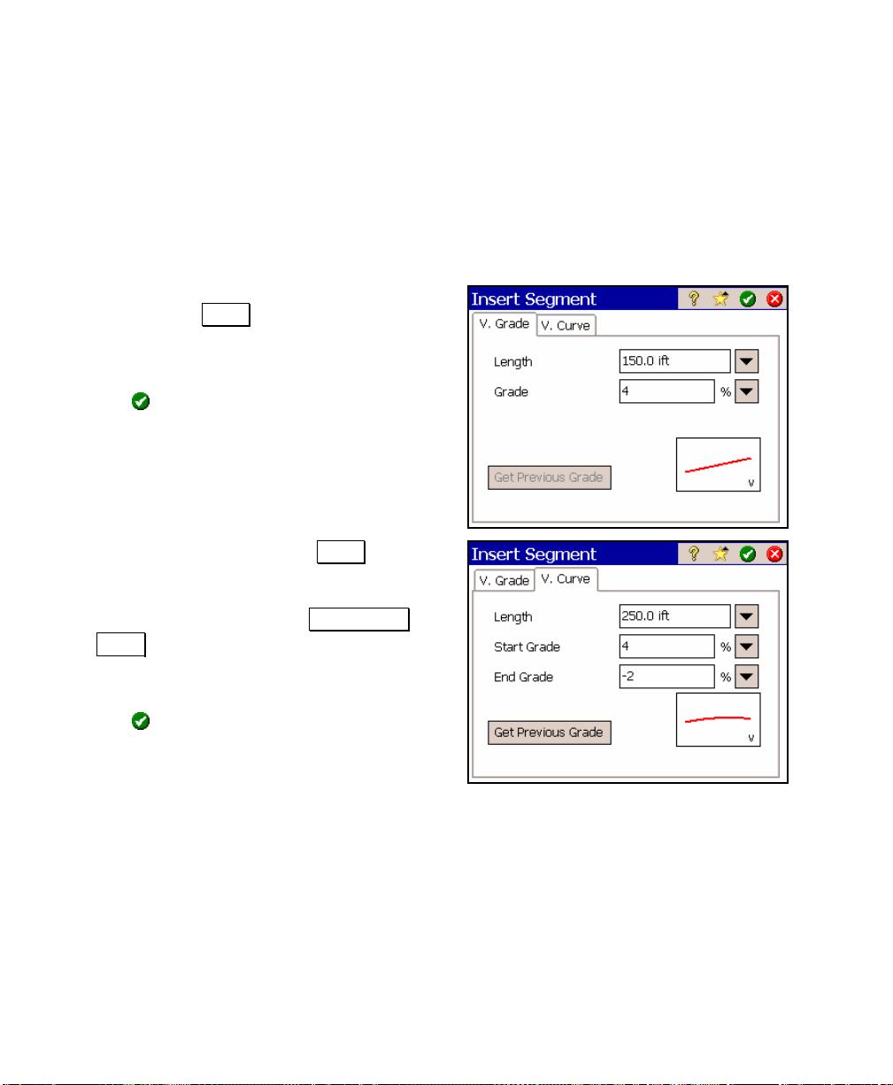
User’s Manual

Vertical Alignment

We have now added all available horizontal segment types. Next, we will define the vertical alignment.

Since the horizontal and vertical alignments are defin ed independently of each other, the first vertical segme nt that is defined will start at the same POB defined above in Step 3.

13. Tap the VAL (Vertical Alignment) tab and then tap the Insert button.

14. Tap the V. Grade tab to insert a grade. Enter a Length of 150 and a Grade of 4%.

15. Tap alignment.

16. With End selected, tap the Insert button again and then tap the V. Curve tab to insert a parabolic vertical curve. Enter a

Length of 250 and tap the Get Previous

Grade to the ending grade of the previous

section. Enter an End Grade of -2%.

17. Tap alignment.

to add the segment to the vertical

Grade button to automatically set the Start

to add the segment to the vertical

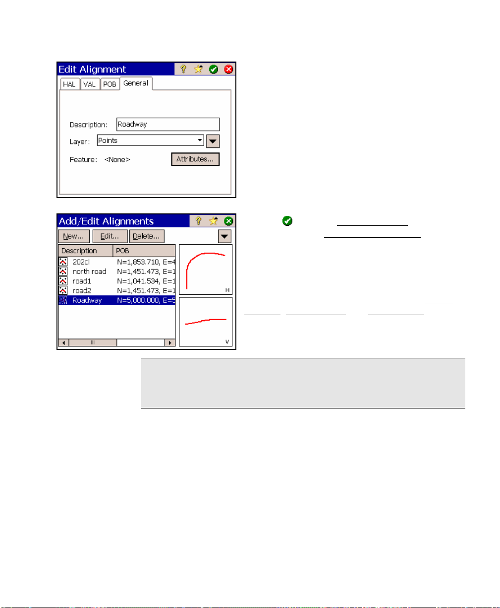
Getting Started

18. Tap the General tab and enter a Description of Roadway.

19. Tap

from the Edit Alignment

return to the Add/Edit Alignments

screen to

screen where the new alignment is stored and displayed.

You have now created a new alignment using all the available types of segments. You can select the new alignment for use in the Offset Staking, Offset Points and Offset Lines routines.

Note: If the horizontal and vertical alignments end at different stations, they can only be processed in the staking routines as far as the end of the shortest alignment.

Conventional Fieldwork

This section will explain how to get started using Survey Pro to collect data from a total station and perform stake out. It is assumed that you are familiar with the operation of your total station. (GPS surveying begins on Page 187.)

The first section describes the backsight setup procedures for var ious scenarios. The next section walks you through the steps involved to setup and perform a simple side shot and traverse shot. The third section walks you through a simple point-staking example.

The remainder of the chapter illustrates the procedures to perform the more complex routines in the Survey Pro software in a step-bystep manner. They are intended to explain only how to use a particular routine without the need for you t o enter any specific values to read through the example.

When beginning any job, the setup is the same; you need to establish an occupy point and a backsight.

The occupy point is the point where you will setup the total station. The coordinates for the occupy point must exist in the curr ent job or active control file. They can be assumed coordinates; known coordinates; or computed with the resection routine. (Control files and the resection routine are discussed later.) Any point in the current job can be an occupy point.

Once an occupy point is established, the second reference you need is a backsight point or direction. This can be in the form of a point stored in the current job, or an azimuth or bearing.

The horizontal angles recorded during data collection are relative to the backsight. If a point is not available in the job to use as a backsight, you can assume a backsight direction or you can use the solar observation routine, described later, to establish a backsight.

The scenarios below will describe four different possibilities for defining a backsight.

User’s Manual – Conventional Mode

Scenario One

You know the coordinates and locations for two poi nts on your lot and want to occupy one and use the other as a backsight.

Solution

1. Create a job using the coordinates for one of the kn own points as the first point.

2. Use the Edit Points coordinates for the remaining known point.

3. From the Backsight Setup point number of one known point and setup the total station over that point.

4. Toggle the .BS Direction. / .BS Point. button to BS Point. and enter the point name for the second known point in that field.

20. Aim the total station toward the other point, zero the horizontal angle on the instrument, and tap Solve , then

Always Prompt for Backsight Check option is checked in the Job > Settings > General screen, you will be prompted to check your

backsight.

You are now ready to start your survey.

routine to add a second point using the

screen, set the Occupy Point field to the

(close). If the

Scenario Two

You have found two points on your lot and know the azimuth between them, but you do not have coordinates for either.

Solution

1. Create a job using the default coordinates for the first point.

2. From the Backsight Setup point that was just created.

3. Setup the total station over the point where the known azimuth is referenced.

4. Toggle the .BS Direction. / .BS Point. button to BS Direction. and enter the known azimuth to the second point here.

screen, set the Occupy Point field to the

Conventional Fieldwork

5. Aim the total station toward the second point, zero the horizontal angle on the instrument, and tap Solve , then

You are now ready to start your survey.

(close).

You may want to take a side shot from the Traverse Sid eshot to the backsight point so that you have coordinates for it. The horizontal angle would remain at zero during this shot.

If you later find true State Plane coordinates for any o f the points in your job, you can use the Translate coordinates accordingly.

routine to adjust all the

screen

Scenario Three

You have one point established on your lot and you know the azimuth to an observable reference.

Solution

1. Create a job using the coordinates of the established point for the first point. If the coordinates are unknown, accept the default coordinates.

2. From the Backsight Setup point that was just created.

3. Setup the total station over the established point.

4. Toggle the .BS Direction. / .BS Point. button to BS Direction. and enter the azimuth to the observable reference here.

screen, set the Occupy Point field to the

5. Aim the total station toward the observable reference, zero the horizontal angle on the instrument, and tap Solve , then (close). If the Always Prompt for Backsight Check option is checked

in the Job > Settings > General screen, you will be prompted to check your backsight.

If you later find true State Plane coordinates for any o f the points in your job, you can use the Translate coordinates accordingly.

routine to adjust all the

User’s Manual – Conventional Mode

Scenario Four

You have only one known point on a job.

Solution

You have two options in this situation. One, you can assume an azimuth for an arbitrary backsight reference and rotate the job later using the Rotate orientation.

Secondly, you can use the Sun Shot routine to determine an azimuth to an arbitrary reference.

routine once you have determined the actual

Summary

In general, you would follow these steps when you begin working on a job.

1. Create a new job or open an existing job.

2. Setup over the Occupy Point.

3. Aim the total station toward the backsight and zero the horizontal angle on the instrument.

4. Fill in the Backsight Setup If the Always Prompt for Backsight Check option is checked in the Job > Settings > General screen, you will be prompted to check your backsight.

5. Start your survey.

Note: You should enter the correct Height of Instrument and Height of Backsight distances in the Backsight Setup screen if you plan to check

your backsight using the Check by Distance routine.

screen and tap Solve , then (close).

Conventional Fieldwork

Note: If the Backsight Circle displays a non-zero value, the angle displayed is subtracted from all horizontal angles that are read during data collection and the resulting points are adjusted accordingly. This will happen after survey with true azimuths or performing stakeout in a special mode. If you do not want this to happen, you should change this value to zero from the Backsi ght

Circle dialog box by tapping the Backsight Circle button.

Most non-staking related data collection is performed from the Traverse / Sideshot

screen. When you take a shot using the Traverse button, the routine expects that you will eventu ally be occupying the foresight that you are shooting and backsighting your current occupy point. When you are ready to setup on the next poi nt, the occupy, foresight and backsight points will automatically be updat ed accordingly.

After taking a shot using the Side Shot button, the routine does not expect the total station to be moved before the next shot and will therefore only automatically advance the foresight point.

User’s Manual – Conventional Mode

Data Collection Example

This section illustrates the necessary setup and usage of the Traverse / Side Shot screen, which is the primary screen used during data collection. We will create a new job and manually add another point to the job to use as a backsight. We will run in manual mode so the shot data must be entered manually. This example and the f ollowing stakeout example are the only examples that are designed where the user should follow along and enter the values in their data collector as they are provided in the example.

Setup

1. Create a new job. a. From the Main Menu

Open / New .

b. Tap New… to open the Create a New

Job screen

c. Enter any job name that you wish in

the Job Name field and tap Next > .

, select File ,

Conventional Fieldwork

d. For this example, simply accept the

default job settings and tap Next > .

Note: When creating a new job, it is important that the Units for Distances field be set to the correct units. This allows you to seamlessly switch between different units in mid-job.

Problems can arise if these units are inadvertently set to the incorrect units prior to

entering new data. For example, assume you created a control file by hand-entering a list of co ordinates in a new job where the job was set to International Feet and the coordinates were in US Survey Feet. Now assume you created another new job and correctly set it to US Survey Feet. If you then selected the previous job as a control file for the new job, the display of a ll of the coordinates in the control file would be conv erted from Feet to US Survey Feet.

e. Accept the default coordinates for the

first job point by tapping Finish .

User’s Manual – Conventional Mode

2. Check the Job Settings. a. Tap Job , Settings from the Main

Menu to open the Settings screen.

b. Select the Instrument card if it is not

already selected and make sure the Manual Mode profile is activated. If the

symbol is not shown next to it, select

Manual Mode and tap Activate .

c. For this example, select the Surveying

Settings card and un-check all the checkboxes.

d. Tap

to save the job settings.

3. Add a backsight point to the job. a. Select Job , Edit Points from the Main

Menu.

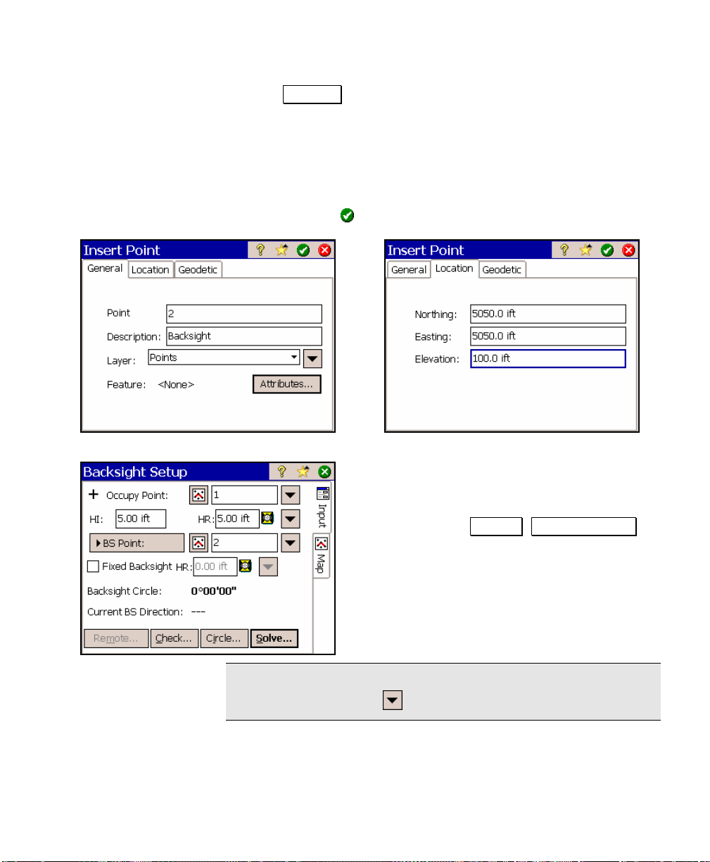
Conventional Fieldwork

b. Tap Insert… and enter a new point using the General and

Location cards with the following values, as shown: Point Name: 2 Northing: 5050 Easting: 5050 Elevation: 100 Description: Backsight

and then tap

4. Set up your backsight. In this example, we will set up on Point 1 and backsight Point 2, which was just created.

a. Access the Survey , Backsight Setup

screen.

b. In the Occupy Point field, enter 1 as the

point name.

Tip: You can also select an existing point from a map view or from a list by using the power button.

User’s Manual – Conventional Mode

c. Enter an HI and HR of 5 feet each. d. Toggle the .BS Direction. / .BS Point. button to BS Point. and

enter 2 as the point name.

e. Leave the Fixed HR at Backsight field unchecked. f. Tap Solve… to open the Backsight

Solved screen.

g. Confirm that the BS Circle value is zero.

If not, change it to zero.

h. Tap the Send Circle button. This

would normally zero the horizontal angle on the instrument and is a required step to properly exit from the screen.

i. Tap

to exit from the Backsight Solved screen. The map view will open showing your current setup.

j. Tap

(close) to continue.

Conventional Fieldwork

Performing a Side Shot

5. Access the Survey , Traverse / Sideshot screen and fill in the appropriate fields. The backsight information is displayed at the top of the screen. At this point, it is assumed that your total station is over the occupy point and its horizontal angle was zeroed while aiming toward the backsight.

a. In the Traverse / Sideshot

the following data if not already entered:

Foresight: 3 Description: SS HR: 5

These values will define the point name, description, and rod height for the next point that is stored.

b. Assuming that the total station is aiming toward the prism,

which is located over the foresight, tap Side Shot . This would trigger the total station to take a shot, compute coordinates for the new point and store it. Since we are running in manual mode, we will enter the shot data from the keypad.

c. Enter the following data:

Angle Right: 70 Zenith: 90 Slope Dist: 100

and then tap computed and stored. The Foresight point will automatically advance to the next available point name and the information from the last shot is displayed on the screen.

. The new point is

screen, enter

User’s Manual – Conventional Mode

d. You can see a graphical representation

of the previous shot by tapping the Map tab. See Page 22 for more information on the Map View

Performing a Traverse Shot

6. The steps involved in performing a traverse shot are nearly identical to performing a side shot. The diff erence is you must specify if you plan to move the total station to the current foresight point after the shot is taken.

a. Tap the Input tab of the Traverse /

Sideshot. The Foresight point should now be updated to 4.

b. Assuming that you are now aiming the

total station at a prism located over the foresight point, tap Traverse . This would trigger the total station to take a

shot, compute coordinates for the new point and store it. Since we are running in manual mode, we will enter the shot data from the keypad.

c. Enter the following data:

Angle Right: 45 Zenith: 90 Slope Dist: 50

and then tap

Conventional Fieldwork

d. The new point is computed and stored

and the Traverse Now or Later

prompt will open, shown here, asking if you want to advance to the new point now or later. For this example, tap the

.Traverse Now. button. The New

Occupy Point dialog box will open, shown here, which displays details of the new setup. You can see that the previous foresight point is now the current occupy point and the previous occupy point is now the current backsight point.

e. Since we are running in manual mode

and cannot send data to an instrument, tap

(close). You will notice at the top

of the Traverse Sideshot

screen that the occupy point has been updated to 4, the backsight is updated to 1, and the foresight is updated to 5, which is the next available point name.

Note: If you select to traverse later, the traverse point is still stored, but you will then have the opportunity to shoot additional side shots before you advance to the next point. This is useful when you want to shoot the traverse shot first, before any settling occurs to the tripod. In that situation, when you are ready to advance, you would tap

Traverse again where you would then answer to a prompt that asks if you are ready to advance or re-shoot the travers e point. (If you select to re-shoot the traverse point, the previous traverse point is stored as a side shot.)

User’s Manual – Conventional Mode

When out in the field, you would now move your total station over the new occupy point, aim it toward the previous occupy point (the current backsight), enter the correct instrument height in the Height

of Instrument field and tap .Send Circle to Instrument . This would update the Traverse / Side Shot screen and set the total station’s horizontal angle to zero where you are then ready to collect more data.

You have now created a job, checked the settings, setup a backsight and collected data in the form of a side shot and a traverse shot. If at any time you want to view the coordinates of your points, you can do

so from the Job , .Edit Points screen.

Data Collection Summary

1. Open or create a job.

2. Check the job settings.

3. Setup a backsight.

4. Collect data in the form of traverse shots or side shots.

Conventional Fieldwork

Stakeout Example

When setting up to perform stakeout, the requirements are nearly the same as with data collection. You need an existing occupy point, backsight point or direction, and a foresight. The main difference is existing points are being located during stakeout rather than new points being collected.

In the example below, all of the steps required to perform a simple point-staking job are explained from th e initial setup to the staking itself. For consistency, this example assumes you are running Survey Pro in manual mode so the shot data will need to be input from the keypad. Since the software behaves differently in manual mode compared to when using a total station, the differences are noted where applicable.

For this example we will use the job that was created with the Traverse / Side Shot Example, above. When staking the first point, we will take two shots to the prism to "home-in" on the design point. When staking the second point, we will only take on e shot combined with the Store/Tape

routine to store the stake point.

User’s Manual – Conventional Mode

Set Up

1. Open the job that was created in the Traverse / Side Shot Example if it is not already open.

a. From the Main Menu

Open / New screen.

b. Tap the file name that was created

earlier listed in the Open Recent Job list and then tap .Open . The coordinates for that job are shown here.

2. Set the job settings. (Only the settings that affect this example are covered here.)

a. Select Job , Settings from the Main

Menu.

b. Select the Instrument Settings screen

make sure Manual Mode is activated.

c. Select the Surveying Settings screen and confirm that all of

the checkboxes are unchecked.

d. Select the Stakeout Settings screen and make sure the Cut

Sheet Offset Stored field (at the bottom of the screen) is set to Actual Offset.

Note: When performing stakeout, you have the option o f storing cut sheet information. This information is stored in the raw data file, and when using software on a PC, it can be extracted in the form of a Cut Sheet Report.

, select File , Open / New to open the

e. Tap to save the job settings.

3. Setup your backsight. In this example, we will setup on Point 1 and backsight an object with a known azimuth. When connected to a total station, you would setup over your occupy point, aim toward the backsight and zero the horizontal angle in the total station before continuing.

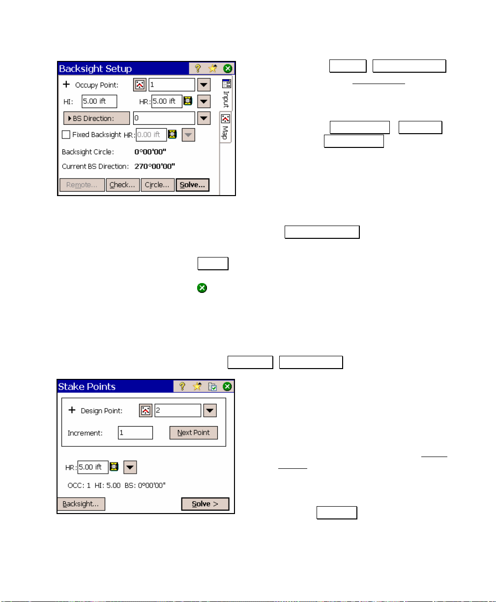
Conventional Fieldwork

a. Access the Survey , Backsight Setup

screen from the Main Menu.

b. In the Occupy Point field, enter 1 as the

point name.

c. Toggle the .BS Direction. / .BS Point.

button to BS Direction. and enter 0 as

the backsight azimuth. d. Enter an HI and HR of 5 feet. e. Leave the Fixed HR at Backsight field

unchecked.

f. Confirm that the Backsight Circle value is zero. If it displays a

non-zero value, tap the .Backsight Circle. button and set it to zero.

g. Tap Solve . A map view will open that shows a graphical

representation of the occupy point and backsight direction.

(close) to continue.

Tap

Staking Points

4. Stake the first design point (Point 2). a. Access the Stakeout , Stake Points. screen. The backsight

information is displayed near the bottom of the screen. At this point, it is assumed that your total station is over the occupy point and its horizontal angle was zeroed while aiming toward the backsight.

b. Enter the following data in the Stake

Points screen:

Design point: 2 Increment: 1 Height of rod: 5

and tap Solve > .

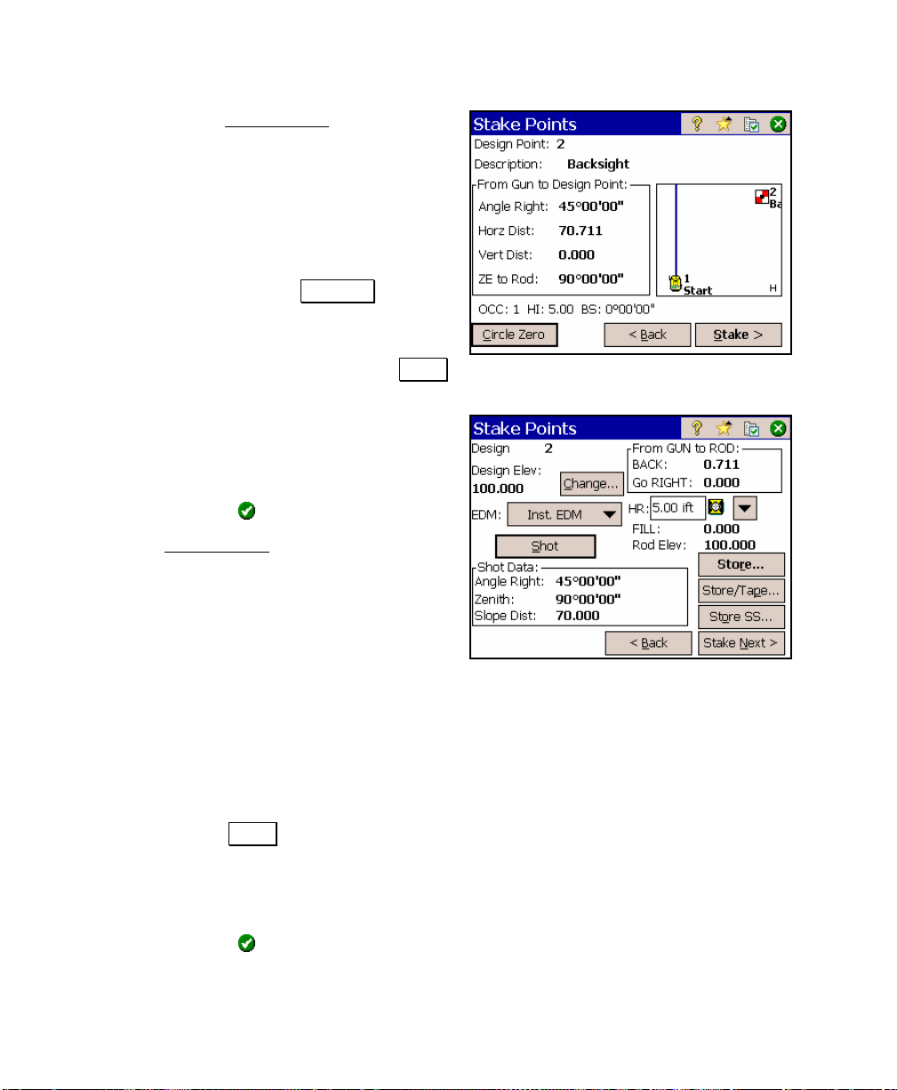
User’s Manual – Conventional Mode

c. The second Stake Points

screen will open that displays all of the information needed to locate the design point. When connected to a total station, you would turn the total station horizontally to 45°00’00", vertically to 90°00’00" and send the rod man out about 70 feet before

continuing. Tap the Stake >. button to continue to the third screen.

d. With a Height of rod of 5, tap the Shot. button. (See the

Reference Manual for an explanation of the other fields.)

e. Enter the following shot data:

Angle Right: 45 Zenith: 90 Slope Dist: 70

and then tap

to continue.

f. The Stake Points

screen will show the necessary COME / GO and Go RIGHT / Go LEFT information that the rod man must move in order to be located over the design point. In this example, the Go RIGHT value indicates 0, which means the rod is precisely on the line between the total station and the design point. The BACK value indicates

0.711, which indicates that the rod must move back (away from the total station) 0.711 feet to be over the design point. The Fill value is zero so no dirt needs to be cut or filled at the rod location to match the design elevation.

g. Assuming the rod has been repositioned, take another shot by

tapping the Shot. button and enter the following new shot data:

Angle Right: 45 Zenith Angle: 90 Slope Dist: 70.8

and then tap

to continue.

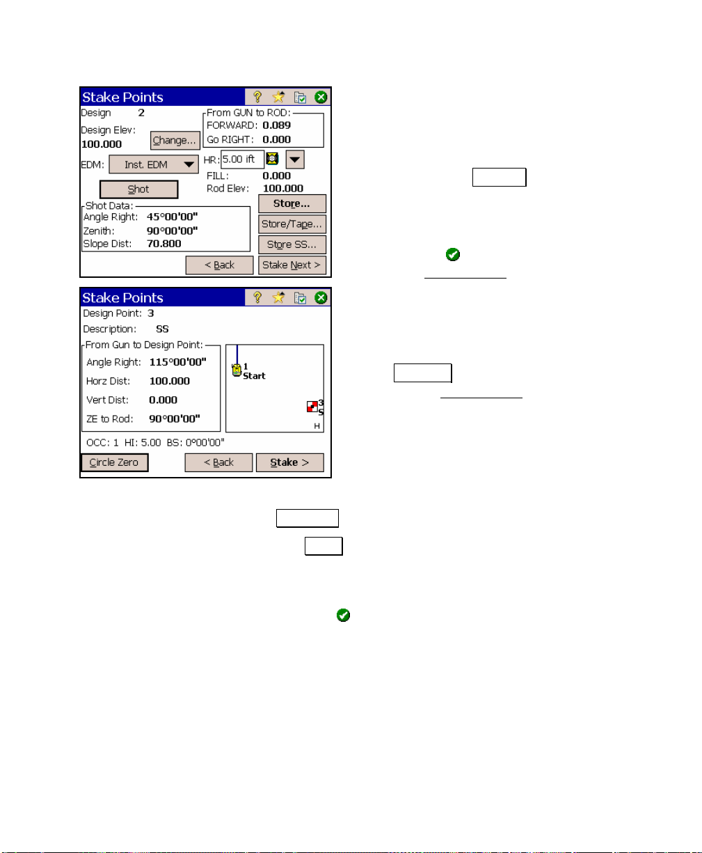
Conventional Fieldwork

h. According to the screen, the rod must

now move FORWARD by 0.089 feet to be over the design point. We will assume that this is close enough and will store the point from this shot by

tapping the Store… button.

i. Enter the following point informatio n:

Point Name: 5 Description: Staked

and tap first Stake Points

. This will return you to the

screen.

5. Stake the next design point. a. We want to stake the next design point

in the project. Make sure 3 is in the Design Point field and then press

Solve > . This will send you to the

second Stake Points screen.

b. The information needed to locate the

next design point is displayed. When connected to a total station, you would turn the total station horizontally to 115°00’00", vertically to 90°00’00" and

send the rod man out about 100 feet before continuing. Tap the .Stake >. button to continue to the third screen.

c. Tap the Shot button and enter the following shot data:

Angle Right: 115 Zenith: 90 Slope Dist: 99.8

and then tap

to continue.

User’s Manual – Conventional Mode

d. The rod needs to move back by 0.2 feet

to be over the design point. Rather than take another shot, we will use a tape measure and place a stake at that

location. Tap the .Store/Tape… button to store the point.

e. Enter the following data in the Store

Point (Tape Offset) Dialog Box:

Point Name: 6 Description: Staked Tape Out/Tape In (+/-): 0.2

and tap that are 0.2 feet further from the total station than the last shot to the prism.

Note: The default value in the Tape Out/Tape In field should put you directly over the design point, assuming you are on line.

Note: Negative Tape Out/Tape In values are toward the total station and positive values are away from the total station.

. This will result in coordinates for the stored point

Point Staking Summary

1. Open a job that contains the design points that you want to stake.

2. Check the job settings.

3. Setup a backsight.

4. Stake the points from the Stake Points

screen.

Conventional Fieldwork

Surveying with True Azimuths

Some people need to collect all of their horizontal angles in the form of azimuths. Survey Pro can help automate this process by computing the backsight azimuth after each new setup in a traverse and updating the backsight circle and total station’s horizontal angle accordingly.

1. You can setup on any existing point and use any other point in the job as a backsight if the coordinate system is properly a ligned with true north. If not, you can occupy any point as long you have a known azimuth to any reference.

2. In the Surveying Settings confirm that the Survey with True Azimuths checkbox is checked.

3. Setup the total station over the occupy point and aim it toward your backsight.

4. Access the Backsight Setup toggle the .BS Direction. / .BS Point. button to BS Direction..

Note: When backsighting on a point, selecting BS Direction can still be used, as described next, making it easier to view the azimuth to the backsight.

5. If backsighting a known azimuth, enter it in the BS Direction field. If backsighting a point, use the shortcut method to enter the azimuth from the occupy point to the backsight point in the BS Direction field. For example, if you are occupying Point 1 and backsighting Point 2, enter 1-2 in the BS Direction field. Once the cursor leaves that field, the computed azimuth will r epl ace what you typed.

6. Tap the Circle… button, enter the backsight azimuth in the Backsight Circle field and tap Send to Instrument (or Set when

running in Manual Mode). This will set the backsight circle as the horizontal angle in the total station and set the same angle as the Backsight Circle value. This angle will then be subtracted from all horizontal angles sent from the total station.

screen ( Job > Settings > Surveying ),

screen; enter the Occupy Point, and

User’s Manual – Conventional Mode

7. Begin your survey. When you traverse to a new point, the New Occupy Point box will open showing you the azimuth computed to the new backsight point from the new occupy point. Once you are setup over the new occupy point, and aiming toward the new backsight point, press the

.Send Circle to Instrument. button to

update the Backsight Circle value and t he horizontal angle on the total station. Repeat this step after setting up on each new traverse point.

dialog

Road Layout

The Road Menu contains a powerful set of routines that allow you to enter and modify road layout information and then stake the road in the field. The road staking routines allow you to stake any part of the road or slope stake the road.

There are four basic components of a road: The Ho rizontal Alignment; the Vertical Alignment; Templates, and a POB. All of these components are described separately below and each is a required component to a complete road definition.

Horizontal Alignment (HAL)

The horizontal alignment, referred to as the HAL, defines the horizontal features of an alignment. It can contain information on straight, curved, and spiral sections of the alignment. Generally the HAL coincides with the centerline of a road, but it is not required to be the centerline. All stationing for an alignment will come from the HAL.

Vertical Alignment (VAL)

The vertical alignment, referred to as the VAL, defines the vertical components of the alignment including grades and parabolic vertical curves.

The VAL is generated in the same way as the HAL. The VAL can be the same length as the HAL, or longer, but it cannot be shorter.

Templates

Templates contain the cross section information for the road. Templates are stored in separate files with a TP5 extension so they can be used with multiple jobs. The templates are broken down into sections, called segments. Each segment contains a specified length, and slope or change in elevation. Templates can contain as many segments as needed, but must have at least one segm ent. Each segment describes one component of the cross section such as the

User’s Manual – Conventional Mode

roadbed, curb face, top of curb, ditch, etc. Each road alignment can contain as many templates as required to define the roadway, but all the templates used on one side of the road must have the same number of segments.

Templates can be further modified using widenings and super elevations:

Widenings are used to widen or to narrow the first segment of a template. The remaining segments of the template are not affected. This feature is intended to be a way of controlling the width of the first segment, typically the roadbed, without having to create and manage additional template files. Widening definitions basically act as two templates that modify the first segment.

Super elevations are used to bank curves in the direction of a turn. A super elevation accomplishes this by changing the slope of the first segment of a template – the slope of any remaining segments will remain unadjusted.

One super elevation defines a begin station and an end station where the slope change begins and where it finishes the transition for one side of a road. Therefore, to bank a two-lane road, four super elevations would be required – one at the beg inning and one at the end of the curve for each side of the road.

A super elevation can either hinge at the outer edge of the first segment, or at the centerline. Hinging at the center results in the elevation of the outer segments to change. Hin ging at the edge results in the elevation of the centerline changin g. Because of this, Survey Pro will only allow you to hinge on edge for one side of a road. If the other side is also super elevated, you will be f orce d to hinge that side at the center so that an abrupt change in elevation does not occur at the centerline.

POB

The POB designates the location in the current job where the alignment starts. The POB can be defined by an existing point or specified coordinates and can be changed at any time. The VAL’s start station elevation will be set from the POP.

Road Layout

Road Component Rules

The following section defines how the various comp onents described above work together to form the road. This information is important because how each component reacts to the other compon ent affects the shape of the resulting road.

Alignments

1. The alignment must have both HAL and VAL segments.

2. The VAL must be equal to, or longer than the HAL.

Templates

1. For each side of the road

• All templates on a particular side of the road must have the same number of segments for. The fist template for each side of the road defines this number.

• The station for the first template for each side must match the starting station of alignment.

• All template stations must be within the station range for the alignment.

• All templates must have at least one segment.

• A template can contain one zero length segment making it

effectively a blank template, but the first segment must be greater than 0.

• Template segments must have a name. The template editor provides fields to enter the segment name.

2. Any two templates without intervening Widening or Super Elevations will transition.

• This means that each template segment will transition at a

linear rate from its existing offset fro m the centerline to the new offset from the centerline as defined by the new template.

User’s Manual – Conventional Mode

3. A template’s first segment slope and/or width w il l be modified when:

• A template is located within a Super Elevation or Widening

definition including starting and ending stations and inside Widening or Super Elevation transition areas.

• Templates will acquire first segment slop e value from the

Super Elevation definition, and/or acquire its first segment width value from the Widening definition.

4. Only one template may occupy any station.

• As little as 0.001 units can be used to separate templates.

Widenings and Super Elevations

1. Super Elevation and Widening stations must be within the station range of the alignment.

2. Super Elevations and Widenings follow the same rules except that the start and end stations of a Super Elevation are defined by:

• Super Elevations will start their transitions at a point equal

to the user defined starting station minus ½ of the starting parabolic transition length if parabolic transitions are used.

• Super Elevations will start their transitions at a point equal

the user defined ending station plus ½ of the ending parabolic transition length if parabolic transitions are used.

3. Super Elevation start slope value and Widening start width value must match the first segment value defined by:

• A previous Super Elevation or Widening. (Priority)

• A previous Template.

4. Super Elevation ending slope value and Widening ending width value must match the first segment value defined by:

• A following Super Elevation or Widening. (Priority)

• A following Template.

Road Layout

• Exception: if the Widening or Super Elevation is the last element in the road, it’s end transition value does not have to match anything.

5. Super Elevation and Widening ending stations must be greater than their beginning stations.

6. Widenings cannot adjust the first segment horizontal distance to or from 0.

7. Super Elevations and a Widenings may overlap, are ind ependent, and do not affect each other.

8. Super Elevations may not overlap other Super Elevations.

• A Super Elevation’s ending station may be equal to a

following Super Elevation’s beginning stati on.

• A Super Elevation’s beginning station may be equal to a

previous Super Elevation’s ending station.

9. Widenings may not overlap Widenings.

• A Widenings ending station may be equal to a following

Widening’s beginning station.

• A Widening’s beginning station may be equal to a previous

Widening’s ending station.

10. Super Elevations may hinge on edge.

• Hinge on edge can only be used for one side of the road f or

any given Super Elevation station range.

• If hinge on edge is used for one side of the road, Super

Elevations must hinge from center on the opposite side of the road over the same station range.

• Hinge on edge will modify the elevatio n of the Center Line.

User’s Manual – Conventional Mode

Road Rules Examples

Figure 1 Overhead view of a template-to-templa te linear transition

Figure 2 Template to Widening Transition

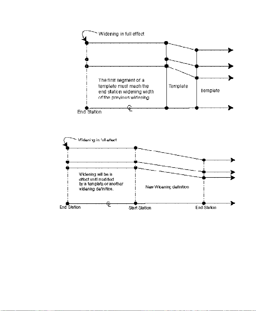
Road Layout

Figure 3 Widening to Template Transition

Figure 4 Widening to Widening Transition

User’s Manual – Conventional Mode

Figure 5 Template Inserted Into A Widening Area

Figure Descriptions

Figure 1 shows an overhead view of a simple transition from one template to another. Notice the linear t r ansition of one template segment end node to the next.

Figure 2 shows an overhead view of a basic template to widening transition. The widening’s first segment width for the start station must match the first segment width of the previous template.

Figure 3 shows a transition from a widening to a template. This example shows that a widening basically defines a new template that has a modified first segment. The modified template (widening) will transition to the next template down the road.

Figure 4 shows the same concept as Figure 3 except another widening is used instead of a template.

Figure 5 depicts how a template can be inserted inside a widening definition. The widening will take prec edence over the first segment so the first segment will maintain the length as defined in the widening definition. However, the segments outside of the first segment now take on the shape of the inserted template. The figure shows a widening where the start width is the same as the end width but having the widening use the same start and end width is not required. The first segment of the template will be adjusted to match

Road Layout

whatever the widening says the width of the first segment should be at the station where the template is inserted.

Also notice in Figure 5 that we have defined a widening with the start width the same as the end width. This can be a handy tool to use if you need to widen the road for a relatively long distance but also need to change the template segments outside the first segment. Using a widening as shown enables you to use any template to modify the outside segments while retaining the same roadb ed (first segment) width.

Super Elevations

The examples above show how widenings interact with templates. Super elevations work with templates in the same way, except instead of the width of the first segment being modified, the cross slope for the first segment is modified.

Creating Templates

The information for a single template is stored in a separate file with a TP5 extension. Template names are limited to eight characters plus the extension so that they can be used in DOS-based data collectors. Each template stores information on the cross section for one side of the road.

A road can have as many templates as necessary, but each side of the road must only use templates with the same number of segments. Once the first template is selected, Survey Pro will only let you select from additional templates that have the same number of segm ents as the first template.

A template can be used on either side of the ro ad. They are not right or left specific. A road could contain only one template, which would be used for both the right and left sides, but can also contain as many templates as necessary.

In this example, we will create a single template that contains a roadbed, a curb, and a ditch. Each segment will be defined in order, starting from the centerline and working t oward the edge.

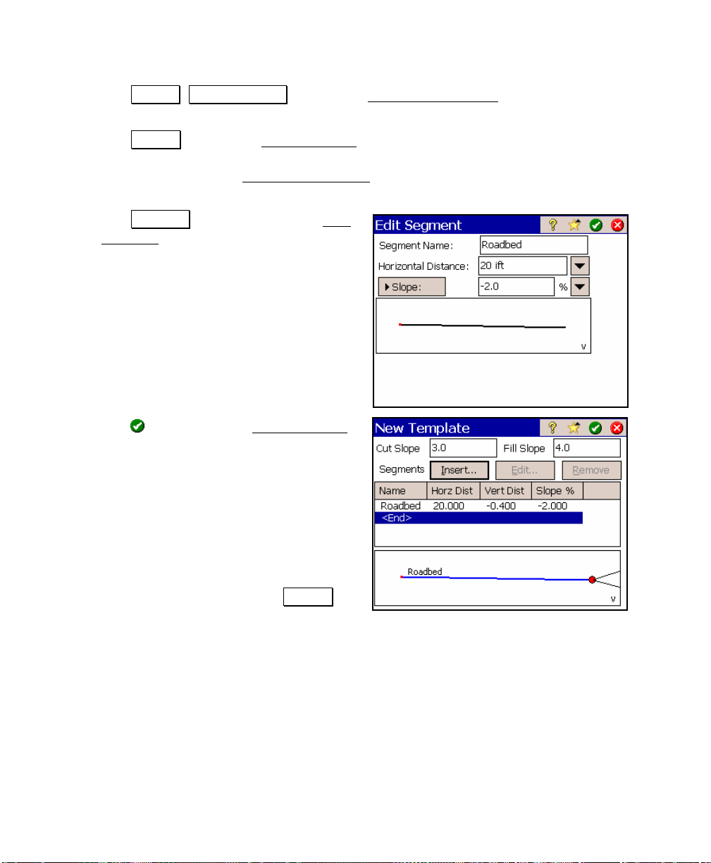
User’s Manual – Conventional Mode

1. Tap Roads , Edit Templates to open the Add/Edit Templates screen.

2. Tap New… to open the New Template

screen. The Cut Slope and Fill Slope values are the slopes to compute the location of catch points with the Road Slope Staking

routine. These

values can also be easily changed from that routine.

3. Tap Insert… . This will open the Edit Segment dialog box. Enter the following information to define the first segment, which will be a 20-foot wide roadbed with a -2% slope.

Segment Name: Roadbed Horizontal Distance: 20 Slope: -2

4. Tap

to return to the New Template screen where the new roadbed segment will appear. A list of segments is displayed. At this point, only the roadbed and <End> will be displayed in the list. Whenever a new template is inserted, it is inserted above the template that is selected in this list. Therefore, to add a new segment to the end of the last segment, <End> should

be selected prior to tapping Insert….

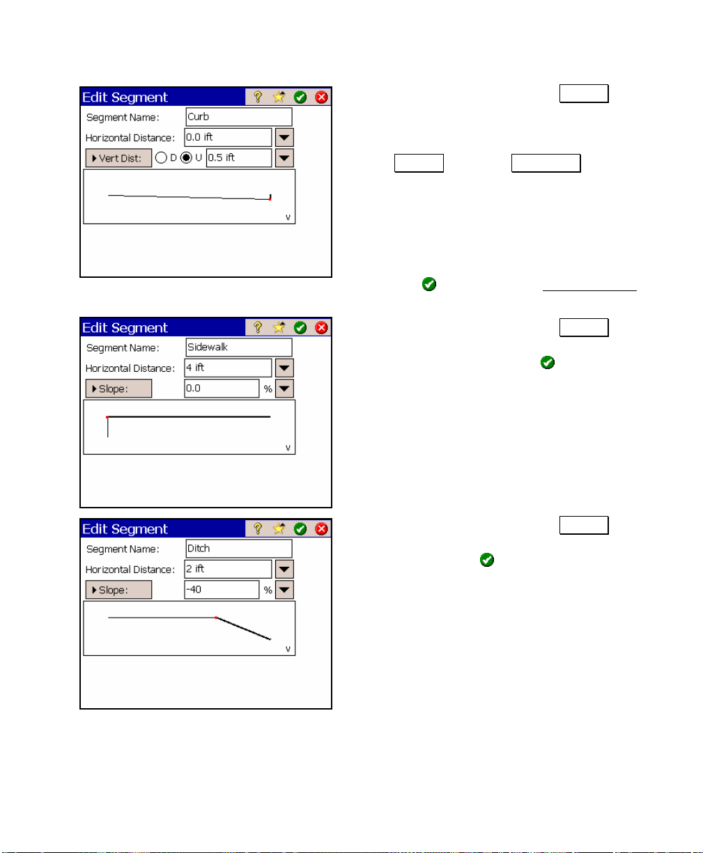
Road Layout

5. With <End> selected, tap Insert… and enter the following data to add a new segment that will describe the face of a curb. Notice you need to toggle the

Slope button to V. Offset and select the ~U radio button to specify that the curb extends upward.

Segment Name: Curb Horizontal Distance: 0 Vert Dist: ~U 0.5

6. Tap

to return to the New Template

screen where the new curb segment will appear.

7. With <End> selected, tap Insert… and enter the following data to add a sidewalk and then tap

Segment Name: Sidewalk Horizontal Dist: 4 Slope: 0

8. With <End> selected, tap Insert… and enter the following data to add a ditch and then tap

Segment Name: Ditch H. Offset: 2 Slope: -40

User’s Manual – Conventional Mode

9. Tap and the Save As Enter T1 in the Name field and tap This completes the creation of a template.

from the New Template screen

screen will open.

Building an Alignment

The Edit Alignments routine is used to create an alignment and is explained in detail starting on Page 44. If you do not currently have any alignments stored on the data collector, either create a simple alignment now that is at least 300 feet long, or follow the instructions that start on Page 44 to create a new alignment that contains each possible type of horizontal and vertical section.

Putting the Road Together

The final step in creating a road that can be point staked or slope staked is to use the Edit Roads routine to combine the template(s) with the alignment and define any widenings and super elevations.

In this example, we will use only one template for the entire road. We will use a widening to add a second lane to the right side of the road and we will add four super elevation definitions to bank the left and right side of a curve.

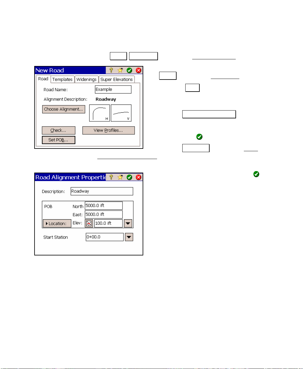
Road Layout

Add Templates to the Alignment

1. Tap Roads Edit Roads to open the Add/Edit Roads screen.

2. Since we are creating a new road, tap New… to open the New Road

3. With the Road tab selected, enter a name

for the road in the Road Name field. In this example, we used Example.

4. Tap the Choose Alignment… button and

select an alignment. In this example, we selected the Roadway alignment created on Page 44. Tap

to continue.

5. Tap the Set POB… to open the Road

Alignment Properties screen to define where the road begins in the job.

screen.

6. Enter the following data then tap

North: 5000 East: 5000 Elev: 100 Start Station: 0+00

User’s Manual – Conventional Mode

7. The next step is to add the templates. We will use the template created earlier to define both sides of the road. Tap the

Templates tab.

8. With <End> selected in the Left column, tap the Add… button. This opens the Add Left Template screen, which allows you to

add a template to the left side of the road.

9. All the available templates will be displayed in the Template column. Select the T1 template, created earlier.

10. Since we will use this template for both sides of the road, check the ; Mirror to Right checkbox and tap

. We now have the minimum number of components to completely define a road: an alignment, and a left and right template.

11. Tap Check… to confirm that the road is okay. You should get a message stating success.

Note: once templates have been added, you can return to the Road card and tap the View

Profiles… button to view the cross-sectional

profile of the road at any station.

Add Widenings

Road Layout

12. Tap the Widenings tab. We will define a widening where a new lane will begin in the right side of the road.

13. Tap <End> in the Right column and then tap the Add… button. This opens the Add Right Widening screen, which allows you to

add a widening to the right side of the road

14. In the Start Station field, enter 0+25. This is where the widening will begin.

15. The length of the widening is 100 feet so toggle the End Station button to Length and enter 100.

16. The starting width of a widening must

equal the width of the first segment of the template that leads into the widening, or if a previous widening leads into it, it must equal the width of the previous widening. Leave the Starting Width field set to its default value of 20.

17. Since we are adding a lane with this widening, enter 40 in the Ending Width field. This widening will now begin at 0+25 and over a 100-foot span; the first segment of the template will increase in width from 20 feet to 40 feet. Bold lines in the map view illustrate the beginning and ending widths of the widening.

18. Tap

to continue.

User’s Manual – Conventional Mode

Add Super Elevations

19. Tap the Super Elevations tab where we will insert a super elevation at the beginning and end of a curve for the left and right sides of the road.

20. With <End> selected in the Left column, tap the Add… button. This opens the Add Left Super Elevation screen, which allows

you to add a super elevation to the left side of the road.

21. We will start the super elevation 100 feet from the beginning of the road so enter 1+00 in the Start Station field.

22. The super elevation will be at the final slope after 25 feet so enter 1+25 in the

End Station field.

23. The start slope must be the same as the slope of the first segment of the template that leads into the super elevation, so leave the Slope 1 field set to -2.

24. We want the ending slope to be 8% so in the Slope 2 field, enter 8 for simplicity, we will not use parabolic transitions so l eav e those fields set to 0.

25. Most super elevations hinge at center so be sure the Hinge on field is toggled to Center and then tap to continue. This will complete the super elevation for the beginn ing of the curve on the

left side of the road.

26. We now need to add a super elevation at the end of the curve on the left side of the road to change the slope back to -2%.

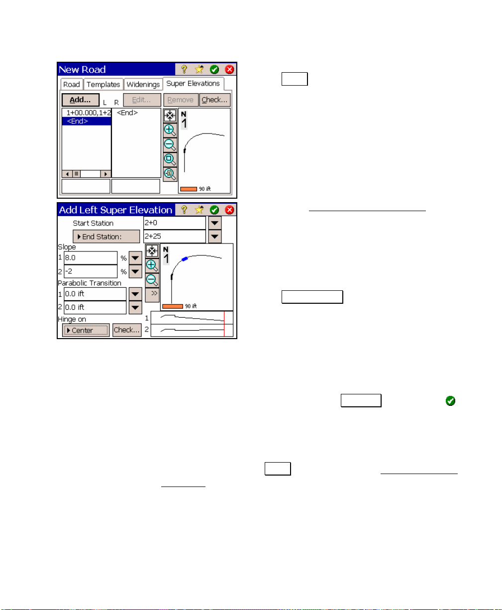
Road Layout

27. With <End> selected in the Left column, tap the Add… button again.

28. From the Add Left Super Elevation

screen we will start the transition out of the super elevation 200 feet from the beginning of the road so enter 2+00 in the Start Station field.

29. The super elevation will return to the original slope after 25 feet so enter 2+25 in

the End Station field.

30. The start slope must be the same as the slope of the road where it leads into the super elevation, so leave the Slope 1 field

set to 8.

31. We want the ending slope to be -2% so in the Slope 2 field, enter

-2. Leave the parabolic transition fields set to 0.

32. Be sure the Hinge on field is toggled to Center and then tap to continue. This will complete the super elevati on entries for the left side of the road.

33. We now need to repeat the above steps for the right side of the road. Tap <End> in the Right column to select that side of the

road and then tap the Add… button to open the Add Right Super Elevation screen.

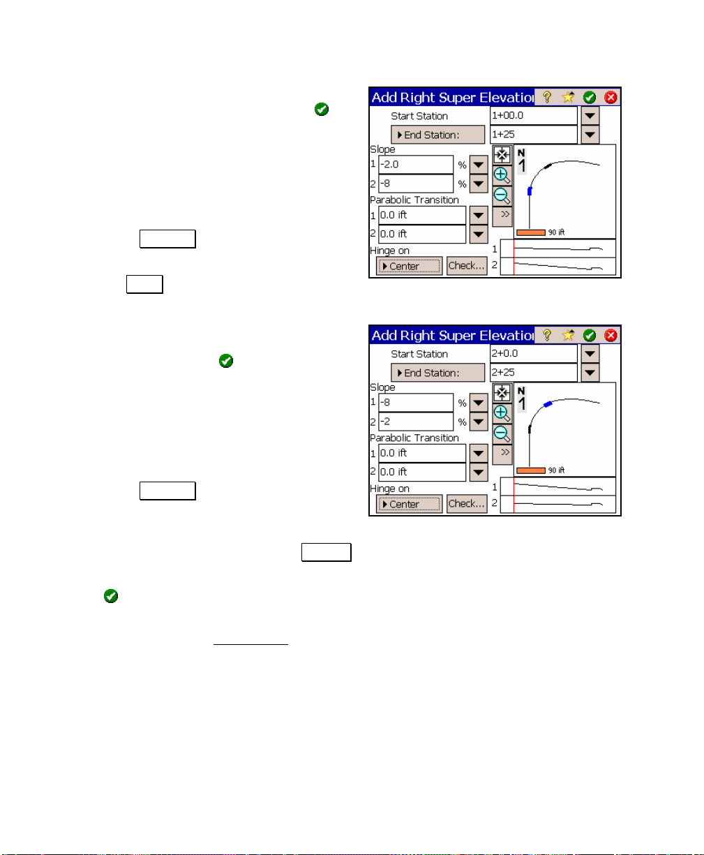
User’s Manual – Conventional Mode

34. Enter the following data just as you did for the left side of the road and then tap

Start Station: 1+0 End Station: 1+25 Slope 1: -2 Slope 2: -8 (note this is a negative value) Parabolic Transition 1: 0.0 Parabolic Transition 2: 0.0

Hinge on: Center

35. With <End> selected in the Right column, tap the Add… button again to add the final super elevation.

36. Enter the following data to describe the second super elevation on the right side of the road and then tap

Start Station: 2+0 End Station: 2+25 Slope 1: -8 Slope 2: -2 Parabolic Transition 1: 0.0 Parabolic Transition 2: 0.0

Hinge on: Center

37. This completes the definition for an entire road including templates, widenings and super elevations. To

make sure there are no errors, tap Check…. You should get a message stating success.

38. Tap

to save the road.

You are now ready to stake the road in the field. Close any open windows to return to the Main Menu

Spectra Precision Survey Pro v4.5 User Manual

Specifications and Main Features

Frequently Asked Questions

User Manual

Table of Contents

Welcome

Getting Started

Manual Conventions

Survey Pro Installation

Registering

Angle and Time Conventions

Azimuths

Bearings

Time

Using Survey Pro

Navigating Within the Program

Command Bar

Parts of a Screen

Input Fields

Output Fields

Input Shortcuts

Quick Pick

Smart Targets

Selecting Smart Targets

Manage Smart Targets

Map View

Basemaps

Basemap Files

Manage Basemaps

The Settings Screen

File Management and ForeSight DXM

Job Files

Raw Data Files

Control Files

Import Control File

External Control File

Description Files

Description Files without Codes

Description Files with Codes

Opening a Description File

Feature Codes

Features

Attributes

Using Feature Codes in Survey Pro

Layers

Layer 0

Other Special Layers

Managing Layers

Working with 2D Points

Polylines

Alignments

Creating an Alignment

Conventional Fieldwork

Scenario One

Scenario Two

Scenario Three

Scenario Four

Summary

Data Collection Example

Setup

Performing a Side Shot

Performing a Traverse Shot

Data Collection Summary

Stakeout Example

Set Up

Staking Points

Point Staking Summary

Surveying with True Azimuths

Road Layout

Horizontal Alignment (HAL)

Vertical Alignment (VAL)

Templates

Road Component Rules

Alignments

Templates

Widenings and Super Elevations

Road Rules Examples

Creating Templates

Building an Alignment

Putting the Road Together