Spectra Precision Survey Pro CE v3.6 User Manual

Download

SURVEY PRO

for Windows® CE

User’s Manual

2002 Tripod Data Systems, Inc.



TRIPOD DATA SYSTEMS SOFTWARE LICENSE AGREEMENT

IMPORTANT: BY OPENING TH E SEALED MEDIA PACKAGE, YOU ARE AGREEIN G TO BE BO UND BY THE TERMS AND CO NDITIO NS OF THE LICENSE AGREEMENT AND LIMITATIONS OF LIABILITY ("Agreement"). THIS AGREEMENT CONSTITUTES THE COMPLETE AGREEMENT BETWEEN YOU AND TRIPOD DATA SYSTEMS, INC. ("Licensor"). CAREFULLY READ THE AGREEMENT AND IF YOU DO NOT AGREE WITH THE TERMS, RETURN THE UNOPENED MEDIA PACKAGE AND THE ACCOMPANYING ITEMS (including written materials and binders or other containers) TO THE PLACE WHERE YOU OBTAINED THEM FOR A FULL REFUND.

LICENSE. LICENSOR grants to you a limited, non-exclusive license to (i) install and operate the copy of the computer program contained in this package ("Program") on a single computer (one central processing unit and associated monitor and keyboard) and (ii) make one archival copy of the Program for use with the same computer. LICE NSOR retains all rights to the Program not expressly granted in this Agreement.

OWNERSHIP OF PROGRAMS AND COPIES. This license is not a sale of the original Program or any copies. LICENSOR retains the ownership of the Program and all subsequent cop ies of the Program made by you, regardless of the form in which the copies may exist. The Program and accompanying manuals ("Documentation") are copyrighted works of authorship and contain valuable trade secrets and confidential information proprietary to LICENSOR. You agree to exercise reasonable efforts to protect LICENSOR'S proprietary interest in the Program and Documentation and maintain them in strict confidence.

USER RESTRICTIONS. You may physically transfer some Programs from one computer to another provided that the Program is operated only on one computer. Other Programs will operate only with the computer that has the same security code and cannot be physically transferred to another computer. You may not electronically transfer the Program or operate it in a time-sharing or service bureau operation. You agree not to translate, modify, adapt, disassemble, de-compile, or reverse engin eer the Program, or create derivative works based on the Program or Documentation or any portions thereof.

TRANSFER. The Program is provided for use in your internal commercial business operations and must remain at all times upon a single computer owned or leased by you. You may not rent, lease, sublicense, sell, assign, pledge, transfer or otherwise dispose of the Program or Documentation, on a temporary or permanent basis, without the prio r written consent of LICENSOR.

TERMINATION. This License is effective until terminated. This License will terminate automatically without notice from LICENSOR if you fail to comply with any provision of this License. Upon termination you must cease all use of the Program and Documentation and return them, and any copies thereof, to LICENSOR.

GENERAL. This License shall be governed by and construed in accordance with the laws of the State of Oregon, United States of America.

LICENSOR grants solely to you a limited warranty that (i) the media on which the Program is distributed shall be substantially free from material defects for a period of NINETY (90) DAYS, and (ii) the Program will perform substantially in accordance with the material descriptions in the Documentation for a period of NINETY (90) DAYS. These warranties commence on the day you first obtain the Program and extend only to you, the original customer. These limited warranties give you specific legal rights, and you may have other rights, which vary from state to state.

Except as specified above, LICENSOR MAKES NO WARRANTIES OR REPRESENTATIONS, EXPRESS OR IMPLIED, REGARDING THE PROGRAM, MEDIA OR DOCUMENTATION AND HEREBY EXPRESSLY DISCLAIMS THE WARRANTIES OF MERCHANTABILITY AND FITNESS FOR A PARTICULAR PURPOS E. LICENSOR d oes not warran t the Program will meet your requirements or that its operations will be uninterrupted or error-free.

If the media, Program or Documentation are not as warranted above, LICENSOR will, at its option, repair or replace the nonconforming item at no cost to you, or refund your money, provided you return the item, with proof of the date you obtained it, to LICENSOR within TEN (10) DAYS after the expiration of the applicable warranty period. If LICENSOR determines that the particular item has been damaged by accident, abuse, misuse or misapplication, has been modified without the written permission of LICENSOR, or if any LICENSOR label or serial number has been removed or defaced, the limited warranties set forth above do not apply and you accept full responsibility for the product.

The warranties and remedies set forth above are exclusive and in lieu of all others, oral or written, express or implied. Statements or representations which add to, extend or modify these warranties are unauthorized by LICENSOR and should not be relied upon by you.

LICENSOR or anyone involved in the creation or delivery of the Program or Documentation to you shall have no liability to you or any third party for special, incidental, or consequential damages (including, but not limited to, loss of profits or savings, downtime, damage to or replacement of equipment and property, or recovery or replacement of programs or data) arising from claims based in warranty, contract, tort (including negligence), strict liability, or otherwise even if LICENSOR has been advised of the possibility of such claim or damage. LICENSOR'S liability for direct damages shall not exceed the actual amount paid for this copy of the Program.

Some states do not allow the exclusion or limitation of implied warranties or liability for incidental or consequential damages, so the above limitations or exclusions may not apply to you.

If the Program is acquired for use by or on behalf of a unit or agency of the United States Government, the Program and Documentation are provided with "Restricted Rig hts". Use, dup lication, or d isclosure by th e Government i s subject to restrictio ns as set forth in subparagraph (c)(1)(ii) of the Rights in Technical Data and Computer Software clause at DFARS 252.227-7013, and to all other regulations, restrictions and limitations applicable to Government use of Commercial Software. Contractor/manufacturer is Tripod Data Systems, Inc., PO Box 947, Corvallis, Oregon, 97339, United States of America.

Should you have questions concerning the License Agreement or the Limited Warranties and Limitation of Liability, please contact in writing: Tripod Data Systems, Inc., PO Box 947, Corvallis, Oregon, 97339, United States of America.

LIMITED WARRANTIES AND LIMITATION OF LIABILITY

U.S. GOVERNMENT RESTRICTED RIGHTS

Survey Pro is a registered trademark of Tripod Data Systems, Inc. Windows and Windows CE are registered trademarks of Microsoft Corporation.

TRADEMARKS

.MAN-CESURVEYPRO 10112002

Table of Contents

Getting Started __________________________________________ 1

Manual Conventions ________________________________1 Installation and Upgrading __________________________2 Angle and Time Conventions ________________________4

Azimuths _________________________________________________ 4 Bearings___________________________________________________ 4 Time______________________________________________________ 4

Starting the Program and Creating a New Job __________5 Navigating Within the Program ______________________7 Hotkeys ___________________________________________9 Parts of a Screen ___________________________________10

Input Fields_______________________________________________ 10 Output Fields _____________________________________________ 10 Input Shortcuts ___________________________________________ 12

The Map View ____________________________________14 The Settings Screen ________________________________15

Navigating to the Screens___________________________________ 16 Instrument Settings Page ___________________________________ 16 Units Settings_____________________________________________ 18 Format Settings ___________________________________________ 18 Files Settings______________________________________________ 19 Surveying Settings_________________________________________ 20 Stakeout Settings __________________________________________ 21 Repetition Settings_________________________________________ 24 Date/Time Settings________________________________________ 25 General Settings___________________________________________ 26

Required Files_____________________________________28

Job Files__________________________________________________ 28 Raw Data Files ____________________________________________ 29

Control Files ______________________________________30

Control File Example ______________________________________ 31

Description Files___________________________________32

Description Files Without Codes_____________________________ 32 Description Files With Codes________________________________ 33 Opening a Description File__________________________________ 34

Feature Codes_____________________________________35

Features__________________________________________________ 36

iii

Attributes_________________________________________________36 Using Feature Codes in Survey Pro___________________________37

Layers____________________________________________38

Layer 0 ___________________________________________________38 Other Special Layers _______________________________________38 Managing Layers __________________________________________ 39

2D / 3D Points ____________________________________ 40 Polylines _________________________________________41 Alignments _______________________________________41

Creating an Alignment _____________________________________42

Fieldwork ______________________________________________47

Scenario One______________________________________________48 Scenario Two______________________________________________48 Scenario Three_____________________________________________49 Scenario Four _____________________________________________50 Summary _________________________________________________50

Data Collection Example____________________________51

Setup_____________________________________________________52 Performing a Side Shot _____________________________________55 Performing a Traverse Shot _________________________________56 Data Collection Summary___________________________________58

Stakeout Example__________________________________59

Set Up____________________________________________________60 Staking Points_____________________________________________61 Point Staking Summary_____________________________________64

Surveying with True Azimuths ______________________65

Road Layout ____________________________________________67

Overview_________________________________________67

Horizontal Alignment (HAL)________________________________67 Vertical Alignment (VAL)___________________________________67 Templates ________________________________________________67 POB______________________________________________________69

Road Component Rules ____________________________69

Alignments _______________________________________________69 Templates ________________________________________________69 Widenings and Super Elevations. ____________________________70 Road Rules Examples_______________________________________72

Creating Templates ________________________________75 Building an Alignment _____________________________77 Putting the Road Together __________________________78

Staking the Road __________________________________83 Slope Staking the Road _____________________________84

DTM Stakeout__________________________________________ 87

Create a DTM or DXF File __________________________87 Set Up the Job _____________________________________88

Select Your Layers_________________________________________ 90 Select a Boundary (optional) ________________________________ 90 Select any Break-lines (optional)_____________________________ 91

Stake the DTM ____________________________________93

View the DTM ____________________________________________ 94

Screen Examples ________________________________________ 97

Import / Export Coordinates________________________97

Importing *.JOB Coordinates________________________________ 98 Importing *.CR5 Coordinates _______________________________ 98 Exporting Coordinates _____________________________________ 99

Repetition Shots __________________________________100

Repetition Settings Screen _________________________________ 100 Repetition Shots Screen____________________________________ 102

Shoot From Two Ends_____________________________104 Offset Shots______________________________________105

Distance Offset Screen ____________________________________ 105 Horizontal Angle Offset Screen_____________________________ 106 Vertical Angle Offset Screen _______________________________ 107

Resection ________________________________________108

Performing a Resection____________________________________ 108

Solar Observations________________________________110

Performing a Sun Shot ____________________________________ 110 What to Do Next _________________________________________ 113

Remote Control __________________________________115

The Remote Control Screen ________________________________ 115 Taking a Shot in Remote Mode _____________________________ 116 Stake Out in Remote Mode ________________________________ 117 Slope Staking in Remote Mode _____________________________ 118

Slope Staking ____________________________________119

Defining the Road Cross-Section____________________________ 120 Staking the Catch Point____________________________________ 122

Intersection ______________________________________125 Map Check ______________________________________126

Entering Boundary Data___________________________________ 126 Editing Boundary Data____________________________________ 127

Adding Boundary Data to the Current Project ________________127

Predetermined Area ______________________________128

Hinge Method____________________________________________128 Parallel Method __________________________________________129

Horizontal Curve Layout __________________________131

PC Deflection ____________________________________________131 PI Deflection _____________________________________________131 Tangent Offset____________________________________________132 Chord Offset _____________________________________________132

Parabolic Curve Layout ___________________________133 Spiral Layout_____________________________________134 Curve and Offset _________________________________135

Define Your Curve________________________________________135 Setup Your Staking Options ________________________________136 Aim the Total Station______________________________________136 Stake the Point ___________________________________________137

Scale Adjustment _________________________________138 Translate Adjustment _____________________________139

Translate by Distance and Direction _________________________139 Translate by Coordinates __________________________________140

Rotate Adjustment________________________________141 Traverse Adjust __________________________________142

Angle Adjust_____________________________________________142 Compass Rule____________________________________________142 Adjust Sideshots__________________________________________143 Performing a Traverse Adjustment __________________________144

Getting Started

TDS Survey Pro for Windows C E is available with different options and sold under the names, Survey Standard, Survey Pro, Survey Pro Robotic, Survey Pro GPS, and Survey Pro Max. Throughout the manual and software, it is simply called Survey Pro. For a listing of which features are included in each product, contact your local TDS dealer.

This manual covers the routines that are available in all of the different software packages except for the GPS routines , which are included with Survey Pro GPS and Survey Pro Max. The GPS routines are covered in a separate manual.

Manual Conventions

Throughout the Survey Pro Manual, certain text formatting is used that represents different parts of the software. The formatting used in the manual is explained below.

Fields

When referring to a particular field, the

Corresponding Value

would see in the software.

is shown with text that is similar to what you

Field Label

, or its

Screens and Menus

When referring to a particular screen or menu, the text is underlined.

Buttons

When referring to a particular button, the text is shown in a

%XWWRQ )RUPDW

, similar to that found in the software.

User’s Manual

Installation and Upgrading

The Survey software that you purchased is shipped pre-installed on the data collector. Upgrading the software is simply a matter of purchasing a registration code that is specifically generated for your data collector. Once entered in the data collector, it will activate the appropriate add-on module.

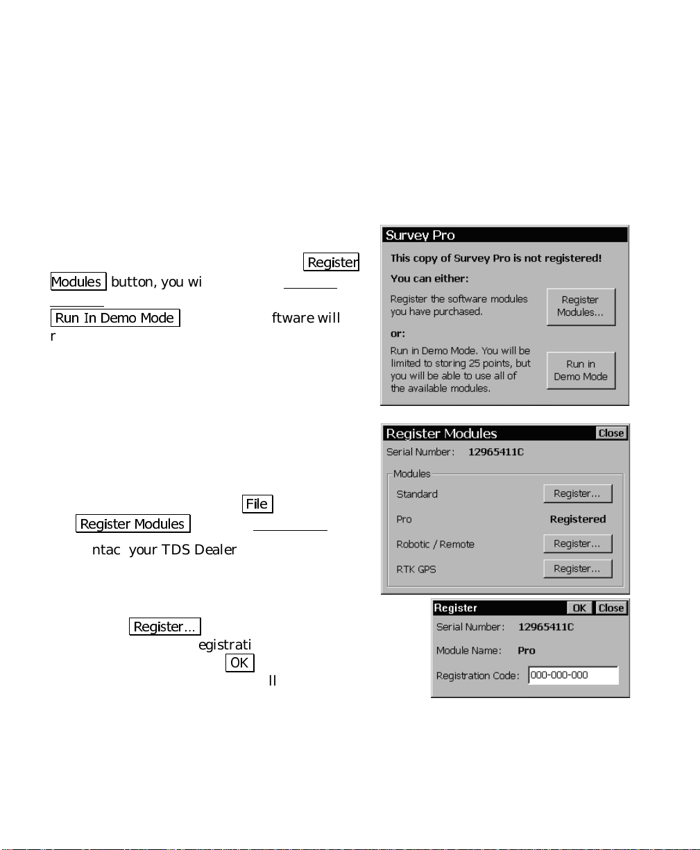
If you start Survey Pro and the Standard Module has not yet been registered, the first screen

shown here will open. If you select the

0RGXOHV

Modules screen, described next. If you select the

5XQ ,Q 'HPR 0RGH

run in demo mode. When running in this special mode, all areas of the software are available. The only limitation is, a job cannot exceed 25 points. If a job is s tored on the data collector that exceeds this limit, it cannot be opened.

Add-on modules can be purchased from your local TDS dealer to upgrade your TDS Survey Software. Upgrading is a quick and easy process and described below.

button, you will access the Register

button, the software will

5HJLVWHU

1. On the data collector, tap

5HJLVWHU 0RGXOHV

2. Contact your TDS Dealer and give him your unique serial number that is displayed on your screen. He will give you a registration number for the module that you purchased.

3. Tap the module, enter the registration number in the dialog box that opens and tap module that you purchased will now be available.

5HJLVWHU«

from the Main Menu

button for the appropriate

)LOH

. All the features for the

Getting Started

Note: You should keep a record of all registration codes purchased in case they need to be reentered at some point.

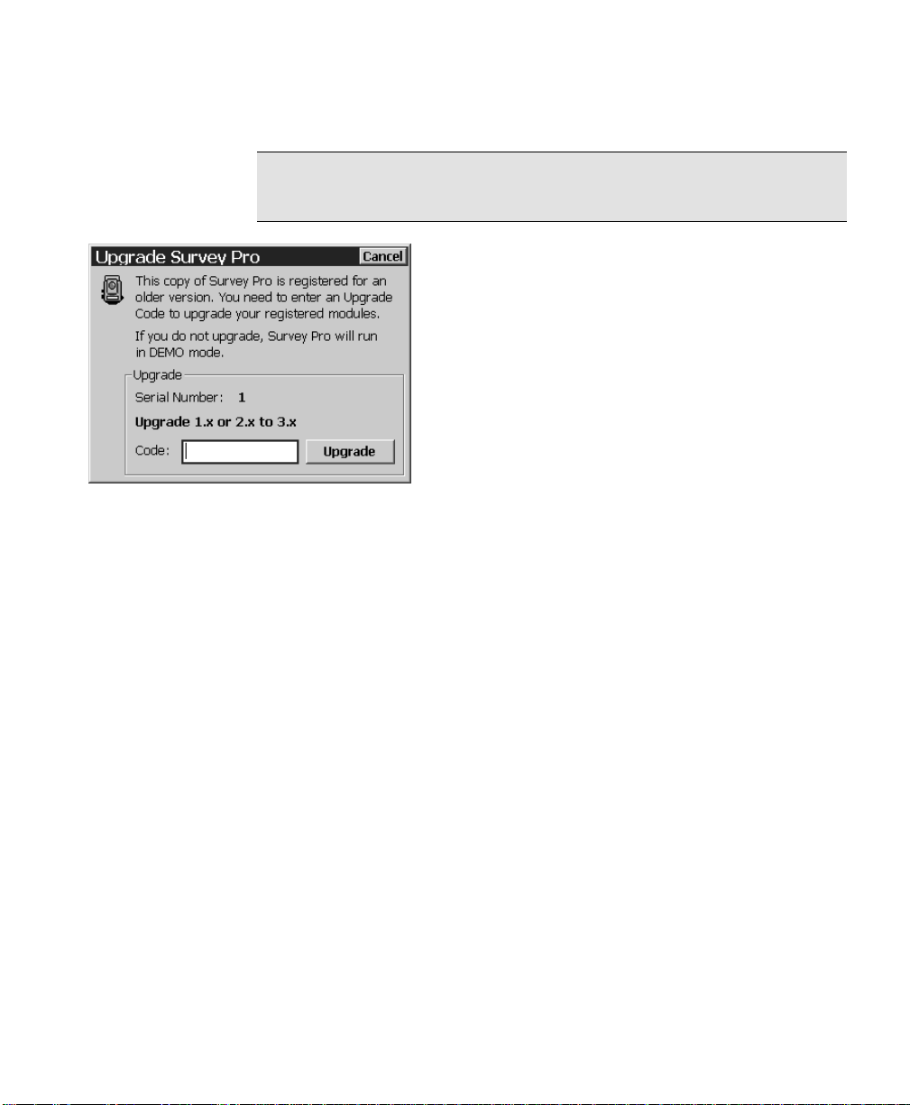
Upgrading from Version 1.x or 2.x to Version 3.0 or later is a chargeable upgrade. Once the new software is installed, the screen shown here will be displayed. A new registration code must be purchased and entered in the software will only run in Demo Mode, as described above. Only one upgrade code is required to upgrade all of the earlier-version modules that were previously registered.

Users that are upgrading to Version 3.0 or later from Version 1.x or 2.x must consider the

following limitations before installing the new software:

• You should have a Ranger with at least 32-MB of onboard memory. The 16-MB models are not sufficient to run the program and store a large job.

field or the

Code

• The Ranger must have Version 2.1 or later of Windows CE installed before installing the new Survey Pro software.

User’s Manual

Angle and Time Conventions

Throughout the software, the following conventions are followed when inputting or outputting angles and time:

Azimuths

Azimuths are entered in degree-minut es-seconds format and are represented as DD.MMSSsss, where:

• DD One or more digits representing the degrees.

• MM Two digits representing the minutes.

• SS Two digits representing the seconds.

• sss Zero or more digits representing the decimal fraction

part of the seconds. For example, seconds.

212.5800

Bearings

would indicate 212 degrees, 58 minutes, 0

Bearings can be entered in either of the following formats:

•

S32.5800W

seconds West.

•

3 32.5800

quadrant 3.

to indicate South 32 degrees, 58 minutes, 0

to indicate 32 degrees, 58 minutes, 0 seconds in

Time

When a field accepts a time for its input, the time is entered in hoursminutes-seconds format, which is represented as HH.MMSSsss where:

• HH One or more digits representing the hours.

• MM Two digits representing the minutes.

• SS Two digits representing the seconds.

• sss Zero or more digits representing the decimal fraction

part of the seconds.

Getting Started

Starting the Program and Creating a New Job

Since Survey Pro runs in the Windows CE operating system, selections and cursor control can be made by simply tapping the screen with your finger or a stylus.

Note: You can temporarily disable the touch-screen if you need to clean it by tapping touch-screen and return to Survey Pro.

You can start the Survey Pro program by double tapping the icon located on the desktop.

- [ ] (space). Tap [ESC] to reactivate the

Ctrl

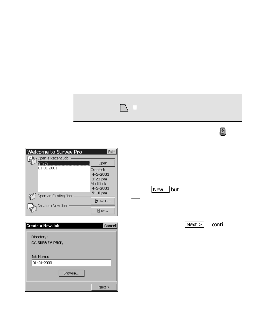
Survey Pro cannot start without a job being open so the Welcome to Survey Pro you want to open a recently opened job, open an existing job, or create a new job. For this example we will create a new job so you can begin exploring the software.

screen will ask if

1. Tap the Job dialog box will open, which prompts you for a job name where the current date is the default name.

2. Either type in a new name or accept the

default name and tap

1HZ«

button. The Create a New

1H[W !

to continue.

User’s Manual

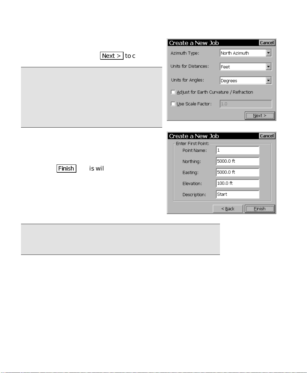
3. Another screen will open where you select some of the job settings. Select the settings

that you desire and tap

Note: When creating a new job, it is important that the correct units. This allows you to seamlessly switch between different units in mid-job. Problems can arise if these units are inadvertently set to the incorrect units when new data is collected.

4. Since all jobs must have at least one point to

Units for Distances

start with, the final screen displays the default point name and coordinates for the first point. Accept the default values by

tapping the new job. You are now ready to explore the software.

)LQLVK

. This will create and store

1H[W !

field be set to the

to continue.

Note: The settings and values entered for a new job become the default values for any subsequent new jobs with the exception of the

Use Scale Factor

setting, which always defaults to off.

Getting Started

Navigating Within the Program

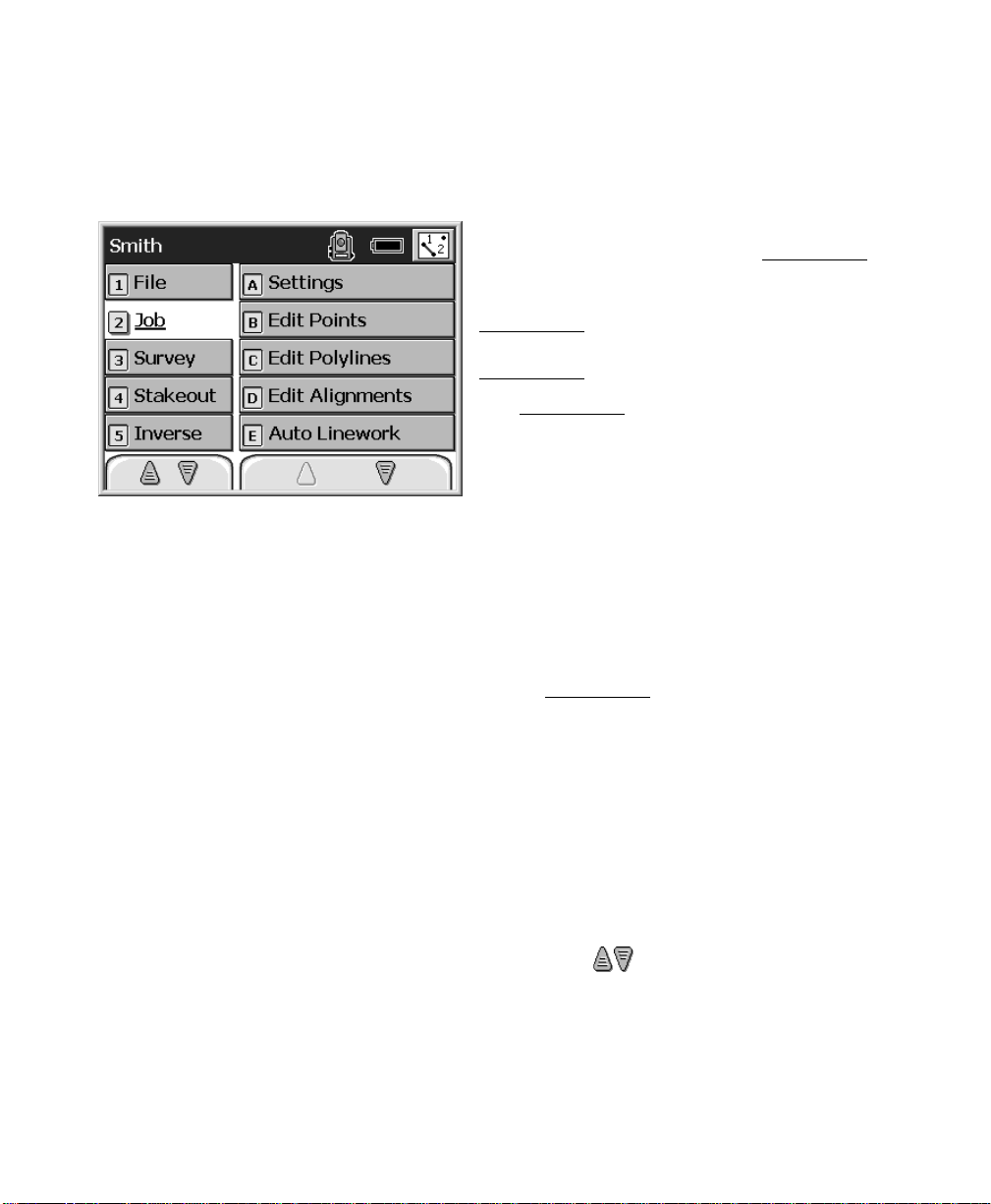
The starting point in Survey Pro, which appears once a job is open, is called the Main Menu shown here. All the screens that are available in Survey Pro are accessed starting from the Main Menu Survey Pro will eventually take you back to the Main Menu

. Likewise, closing the screens in .

The Main Menu left column contains all of the available menus and the column on the right contains the menu items associat ed with the active menu.

When a menu is selected from the left column, the corresponding menu items will become available in the right hand column. When a menu item is activated from the right hand column, the corresponding screen will open. It is from these screens where you do your work.

Navigation through the menus and menu items can be done using any of the methods described below. The best way to become familiar with navigating through the Main Menu

Each menu has a number associated with it, whereas the menu items have letters associated with them. Pressing the associated number or letter on the data collector’s keypad will activate the corresponding menu or menu item.

You can scroll through the list of menus and menu items by using the arrow keys on the keypad. The up and down arrow keys will scroll up and down through the selected column. The other column can be selected by using the horizontal arrow keys.

You can also scroll through the list of menus and menu items by tapping the special arrow buttons bottom of each column. If one of these buttons appears blank, it indicates that you can scroll no further in that direction.

consists of two columns . The

is to simply try each method.

on the screen located at the

When the desired menu item is selected, it can be activated by tapping it or pressing t h e [ Enter] key on the keypad.

User’s Manual

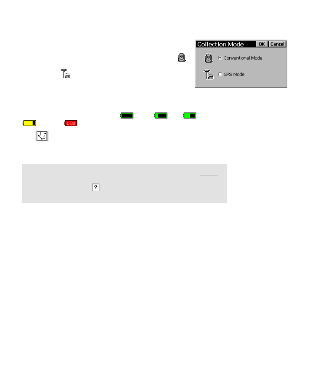
There are three icons in t he Main Menu’s title bar. The first icon indicates which collection mode the software is

running in. When surveying with a total station, the icon is displayed and when surveying with a GPS receiver, the open the Collection Mode can be switched to the other mode.

The battery icon indicates the condition of the data collector’s rechargeable battery. The icon has five variations depending on the level of charge that is remaining:

25% and 5%.

icon is displayed. Tapping this icon will

dialog box where the software

100%, 75% 50%,

The current job when it is tapped. The map view is available from most screens and is discussed later.

Note: Tapping the battery icon is a shortcut to the Microsoft Power Properties screen, which is normally accessed from the Windows CE Control Panel. Tap the button in the title bar of this screen to view the online help.

button in the title bar will access the map view of the

Getting Started

Hotkeys

There are several shortcuts available to qui ckly access a variety of screens no matter where you are at in the software. These shortcuts

are called hotkeys. Each hotkey is activated by holding down the key as you press the associated hotkey on the keypad. Each hotkey is listed below.

Disable Touch-Screen A Calculator B Enter Note D View Points E View Raw Data F View Map G Inverse Point to Point H Corner Angle I Triangle Solutions

Ctrl

J Past Results K Manage Layers L Auto Linework M Horizontal Curve Solution N Vertical Curve Solution O Distance Offset P Horizontal Angle Offset Q Vertical Angle Offset R Traverse / Sideshot S Where is Next Point? Y Remote Control

User’s Manual

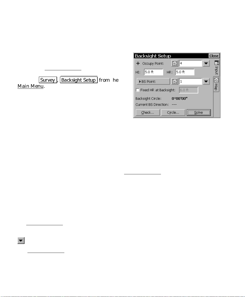
Parts of a Screen

Many screens share common features. To illustrate some of these features, we will examine parts of the Backsight Setup You can access the Backsight Setup

selecting Main Menu.

6XUYH\, %DFNVLJKW 6HWXS

Input Fields

An input field is an ar ea where a specific value is entered by the user. An input field consists of a point label, which identifies the data that is to be entered in that field. It has a rectangular area with a white background, where the data is entered. A field must first be selected before data can be entered in it. You can select a field by tapping on it or pressing the [Tab] key on the data collector repeatedly until it is selected. When a field is selected, a dark border is drawn around it and a blinking cursor is inside the field. In the Backsight Setup screen above, the

Occupy Point

screen, shown here.

screen by from the

field is selected.

Output Fields

Output fields only display information. These fields typically display values in value cannot be changed from the current screen. For example, in the Backsight Setup field.

bold text

Power Buttons

The Backsight Setup screen contains two power buttons. Power buttons are typically used to provide alternate methods of entering or modifying data in an associated field. To use a power button, simply tap it. Once tapped, a dropdown list will appear with several choices.

, do not have a special colored background, and the

screen, the

Backsight Circle

value is an output

Getting Started

The choices available vary depending on with which field the power button is associated. Simply tap the desired choice from the dropdown list.

Tapping the first power button in the Backsight Setup you to specify an occupy point using other methods or view the details of the currently selected point. You should experiment with the options available with various power buttons to become familiar with them.

screen allows

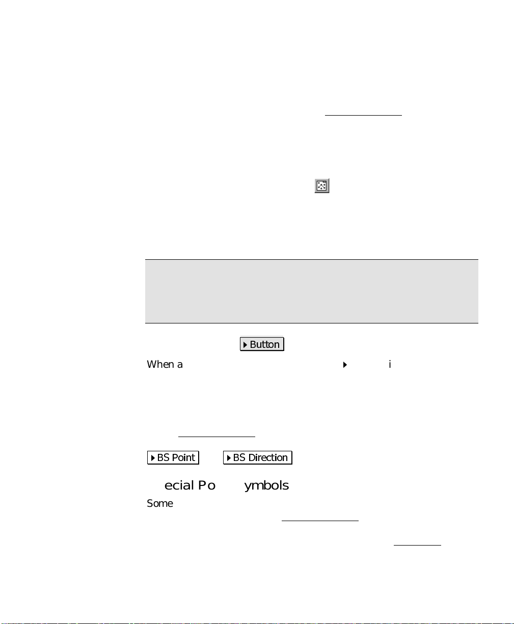
Choose From Map Button

The Choose From Map But ton is always associated with a field where an existing point is required. When the button is tapped, a map view is displayed. To select a point for the required field, just tap it from the map.

Note: If you tap a point from the map view that is located next to other points, another screen will open that displays all of the points in the area that was tapped. Tap the desired point from the list to select it.



Scroll Buttons

When a button label i s preceded with thesymbol, it indicates that the button label can be changed by tapping it, thus changing the type of value that would be entered in the associated field. A s you continue tapping a scroll button, the label will cycle through all the available choices.

%XWWRQ

In the Backsight Setup point or a direction by toggling the scroll button between



%6 3RLQW

and %6 'LUHFWLRQ

screen, the backsight can be defined by a

Special Point Symbols

Some field labels are preceded with a special symbol. For example, the

Occupy Point

represented as a plus symbol when viewing it in the Map View Other symbols are also used to represent other types of points.

field in the Backsight Setup

” The plus symbol indicates that the occupy point is

screen is displayed as “

User’s Manual

Index Cards

Many screens actuall y consist of multiple screens. The different screens are selected by tapping on various tabs, which look like the tabs on index cards. Because of this, each individual screen is referred to as a card. The tabs can appear along the top of the screen or the right edge.

The Backsight Setup and the other is titled

The Settings accessing several screens and is discussed in more detail starting on Page 15.

screen has a variant of the Index Card format for

screen consists of two cards. One is titled

Map

Input

Input Shortcuts

Distances and angles are normally entered in the appropriate fields simply by typing the value from the keypad, but there is a shortcut that can simplify th e entry of a distance or angle.

If you want to enter the distance between two points in a particular field, but you do not know offhand what that distance is, you can enter the two point names that define that distance separated by a hyphen. For example, entering the horizontal distance from Point 1 to Point 2. As soon as the cursor is moved from that field, the horizontal distance between the points will be computed and entered in that field.

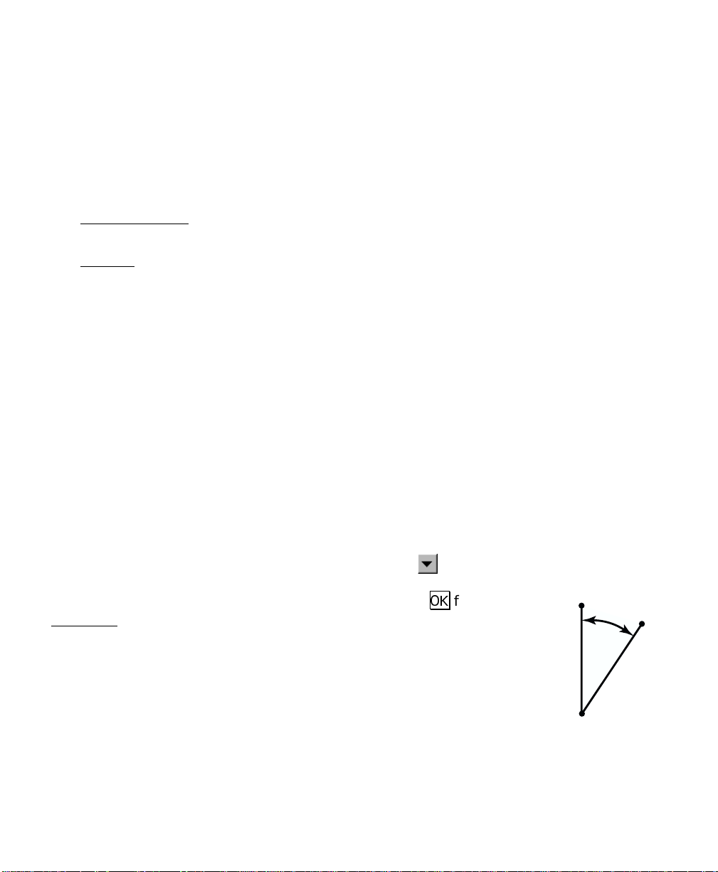
An alternate method to using this shortcut is to tap the button, select define the distance that you want to enter. Once you tap 2. from the Map View, the horizontal distance between the two tapped points will appear in the corresponding field.

Choose from map…

in a distance field would compute

1-2

power

and then tap the two points that

Likewise, there is a similar shortcut to enter angles in fields that accept them. If you wanted to enter the angle, α, from the illustration shown here, you would simply enter appropriate field. As soon as the cursor is moved from that field, the angle formed by the three points entered will be entered in that field. As with specifying a distance, you could also use the power button as described above and tap the poi n ts of the angle in the correct order.

1-2-3

in the

Getting Started

Entering Distances in Other Units

When a distance is entered in a particular field, it is normally entered using the same units that are configured for the current job, but distances can also be entered that are expressed in other distance units.

When entering a distance that is expressed in units that do not match those configured for the job, you simpl y append the entered distance with the abbreviation for the type of units entered. For example, if the distance units for your current job were set to wanted to enter a distance in meters , you would simply append the distance value with an m or M for meters. As soon as the cursor is moved to another field, the meters that were entered will be converted to feet.

The abbreviations can be entered in lower case or upper case characters. They can also be entered directly after the distance value, or separated with a space. The following abbreviations can be appended to an entered distance:

Feet

and you

• Feet:

• US Survey Feet:

• Inches:

• Meters:

• Centimeters:

• Millimeters:

• Chains:

usft

usf in m cm mm

User’s Manual

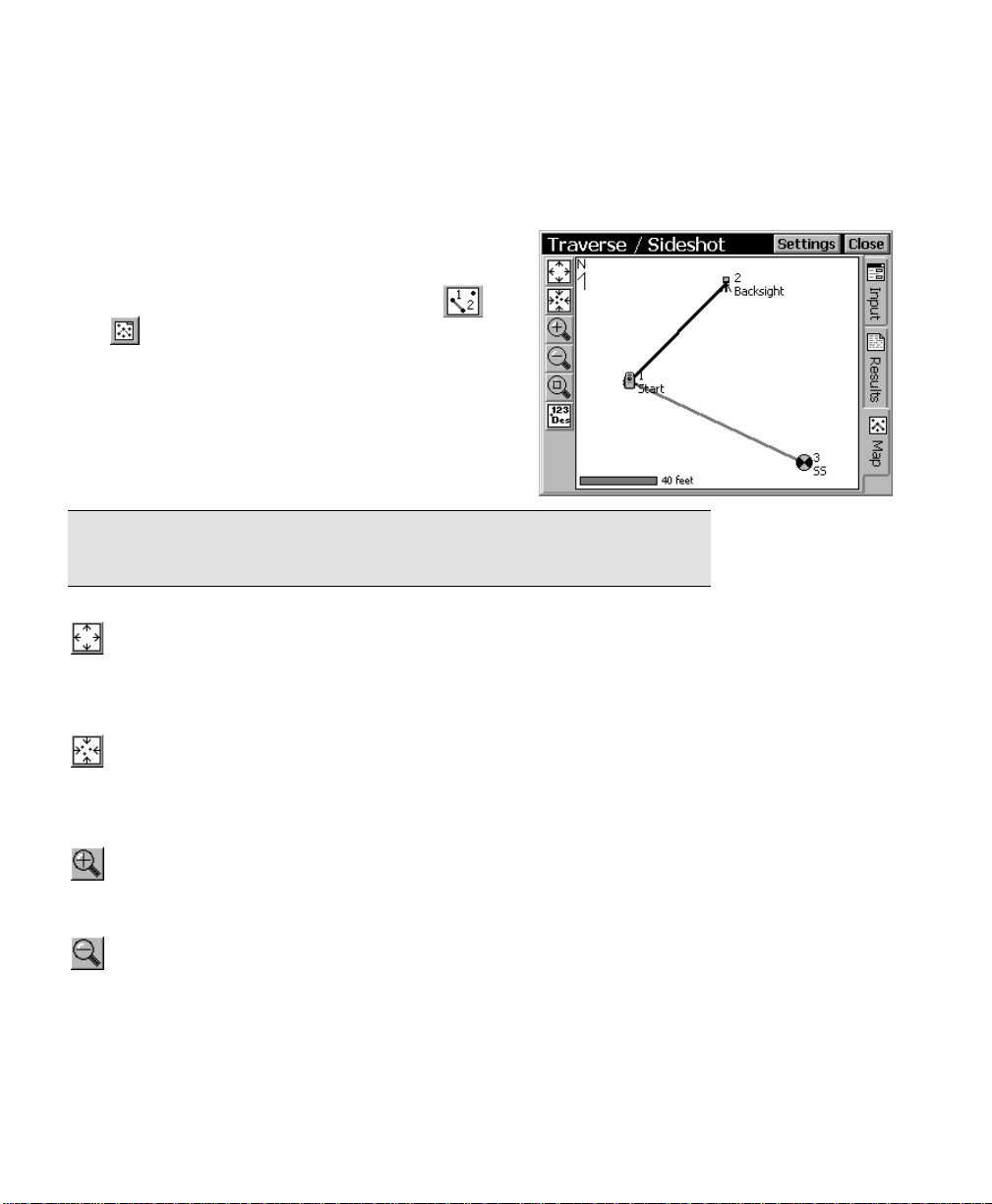
The Map View

Many screens provide access to a map view. The map view is a graphical repres entation of the points and other useful informat ion in the

current job and can be accessed with the and

that indicates the scale of the map view. The buttons along th e left edge of the screen

allow you to manipulate the map view so that it displays what you want to see.

Some map views also display a vertical profile.

Tip: You can pan around your map by dragging your finger or stylus across the screen.

This button will change the scale of the screen so that all the points in the current job will fit on the screen.

buttons. A bar is shown at the bottom

Zoom Extents Button

Zoom Preview Button

When this button is available, it will display only the points that are currently in use.

Zoom In Button

This button will zoom the current screen in by approximately 25%.

Zoom Out Button

This button will zoom the current screen out by approximately 25%.

Getting Started

Zoom Window Button

After tapping this button, a box can be dragged across the screen. When your finger or stylus leaves the screen, the map will zoom to the box that was drawn.

Increase Vertical Scale

This button is only available when viewing a vertical profile. Each time it is tapped, the vertical scale of t h e view is increased.

Decrease Vertical Scale

This button is only available when viewing a vertical profile. Each time it is tapped, the vertical scale of t h e view is decreased.

Display / Hide Labels Button

In some screens, this button will simply toggle the point names and descriptions on and off in a Ma p View open the Map Display Options control over what is displayed in the Map View

, but in other screens it will

screen, which gives you even more

The Settings Screen

The Settings screen is used to control all of the settings available for your total station, data collector, current job, and Survey Pro software.

Most of the settings remain unchanged unless you deliberately change them, meaning the default settings are whatever they were set to last. For example, if you create a new job where you change the direction units from azimuths to bearings and then create another new job, the default direction units for the new job will be bearings.

Survey Pro behaves in thi s way since most people use t he same settings for a majority of their jobs. This way, once the settings are set, they become the default settings for all new jobs and current jobs.

Some settings are considered critical and are therefore stored within the job. The following settings are stored within a job and will

User’s Manual

override the corresponding settings in the Settings opened:

screen when it is

•

Scale Factor

•

Earth Curvature On

•

Units for Survey Data

•

North Angle Units GPS setup information

etc. (Requires GPS Module)

– Surveying Settings Card

Off

(distances) – Units Settings Card

South Azimuth

– Units Settings Card

such as localization, mapping plane,

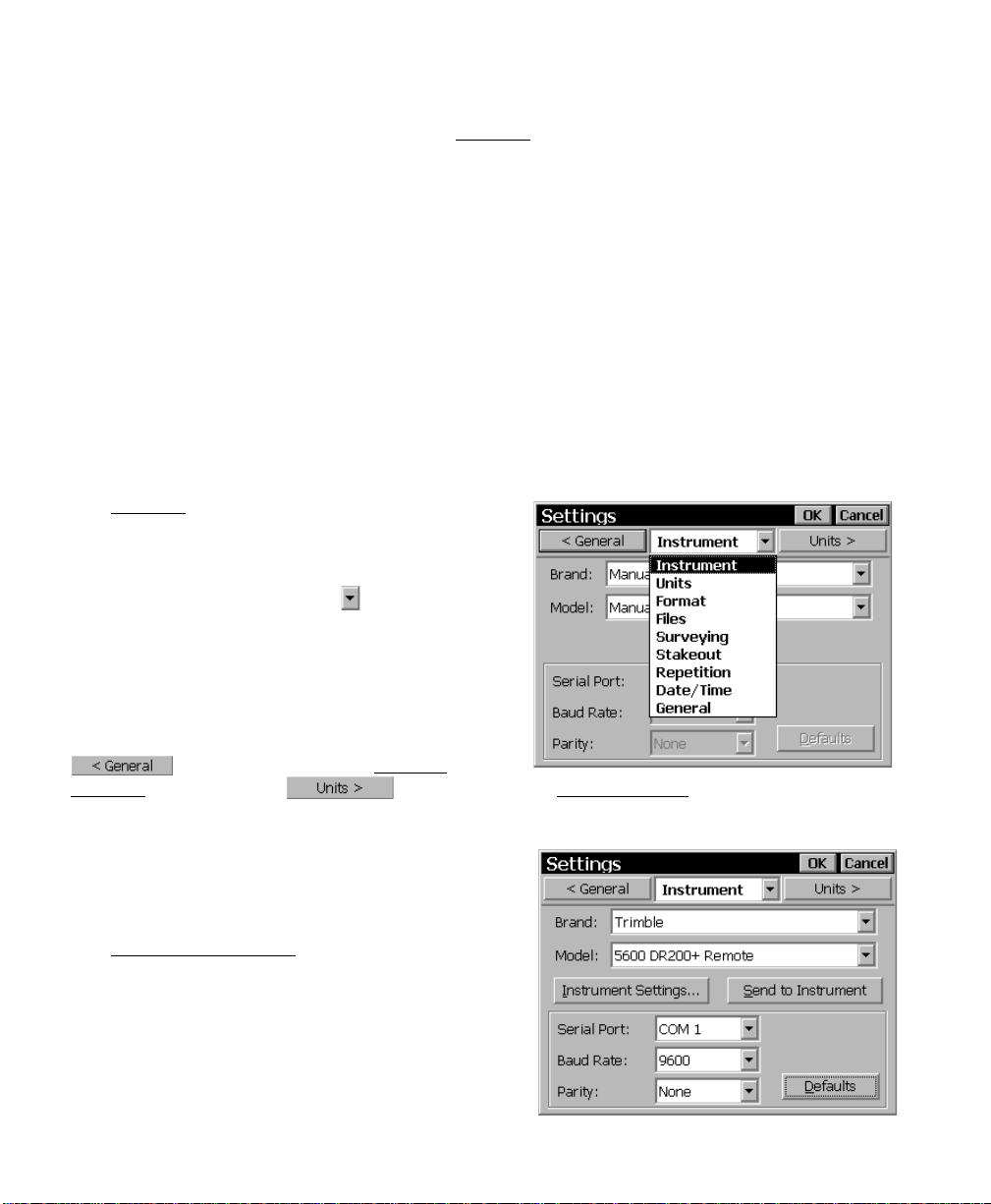
Navigating to the Screens

The Settings screen actually consists of several separate screens where each indivi dual screen contains different types of settings. There are two ways to navigate to the various screens. The first method is to tap the down the list of available screens and then tap on the desired screen from the list to open it. The second method is to tap the buttons to the side of the screen title, which will open the previous or next screen respectively. For example in the screen shown, you could tap

to open the previous (General Settings) screen, or tap to open the next (Units Settings) screen. Repeatedly tapping either of these buttons will cycle through all the available screens.

button to drop

Instrument Settings Page

The Instrument Settings are used to define the type of total station that is being used so it can communicate with the data collector. When your data collector is connected to a total station, the

and

Brand

your total station. If your exact model is not

should be selected to match

Model

Getting Started

listed, you should select from the models that are available until you find one that works.

When set to

Manual Mode

, the data collector will not communicate with a total station. Instead, when a button is pressed that would normally trigger the total station to take a shot; a dialog box will open where you enter the shot data manually from the keypad. When you are learning the software in an office environment, it is usually easiest to set the software to manual mode.

: is where you specify the model of the total station that you are

Model

using from a dropdown list. When a particular model is selected, the default settings for that model are automatically selected. If those setting are changed manually, you can switch back to the default

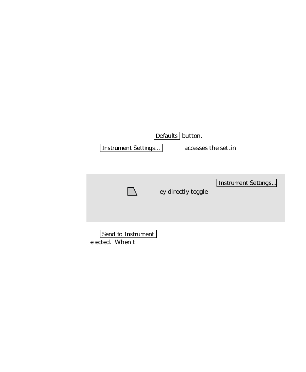
settings by tapping the The

,QVWUXPHQW 6HWWLQJV«

'HIDXOWV

button.

button accesses the settings that are specific for the selected total station model. This screen can also quickly be accessed from anywhere in the program by using the.

Note: The options available after tapping the button, or the

-W hotkey directly toggle settings that are built into

Ctrl

,QVWUXPHQW 6HWWLQJV«

your particular total station. These settings are explained in your total station’s documentation and are not explained in the Survey Pro Manual.

The

6HQG WR ,QVWUXPHQW

button is available when certain models are selected. When this button is available, it should be tapped after turning the total station on. This will send an initializing string to the instrument that will make certain robotic functions work more smoothly.

User’s Manual

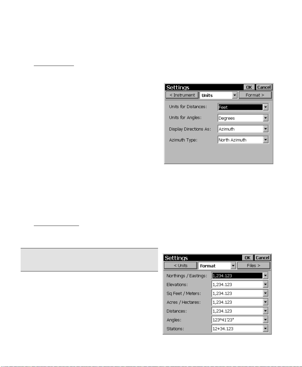
Units Settings

The Units Settings defines the units that are used within the software, including those that are sent from the total station, entered from the keypad and displayed on the screen. You can select the following settings for your job.

Units for Distances

distances as

Units for Angles

angles as

Display Directions As

Bearing

Azimuth Type

Azimuth

Meters, Feet

Degrees

Azimuth

or a

South Azimuth

: defines the units used for

, or

International Feet

: defines the units used for

: defines if you are using a

Grads

: will display directions as

North

Format Settings

The Format Settings defines the precision (the number of places beyond the decimal point) that is displayed for various values in all screens, and how stations are defined.

Note: All internal calculations are performed using full precision.

Northings / Eastings

from zero to six places passed the decimal point for northing and easting values.

Elevations

places passed the decimal point for elevations.

Sq Feet / Meters

to four places passed the decimal point for

: allows you to display from zero to six

: will allow you to display

: allows you to display from zero

square feet or square meter values.

Getting Started

Acres / Hectares

passed the decimal point for acre or hectare values.

Distances

decimal point for distances.

Angles

with angle values.

Stations

formats:

: allows you to display from zero to six places passed the

: allows you to include from zero to four fractional seconds

: allows you to display stations in any of the following

•

12+34.123

the + advances after traveling 100 feet or meters.

•

1+234.123

the + advances after traveling 1,000 feet or meters.

•

1,234.123

: allows you to display from zero to four places

: displays stations where the number to the left of

: displays standard distances rather than stations.

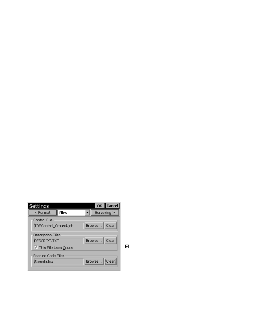
Files Settings

The Files Settings allow you to select a control file or description file to use with the current job.

Control File

: allows you to select a control file to use with the current

job. Control files are discussed in more detail on Page 28.

Description File

description file to use with the current job. Description files are discussed in more detail on Page 32.

This File Uses Codes

;

description file contains codes and associated descriptions. Leave the b ox unchecked if the description only contains descriptions (no codes).

: allows you to select a

: Check this box if the

User’s Manual

Feature Code File

the current job. You can switch b etween different feature code files in mid-job, but if a collected attribute does not match an attribute in the feature code file, it can only be viewed, but not edited.

: allows you to select a feature code file to use with

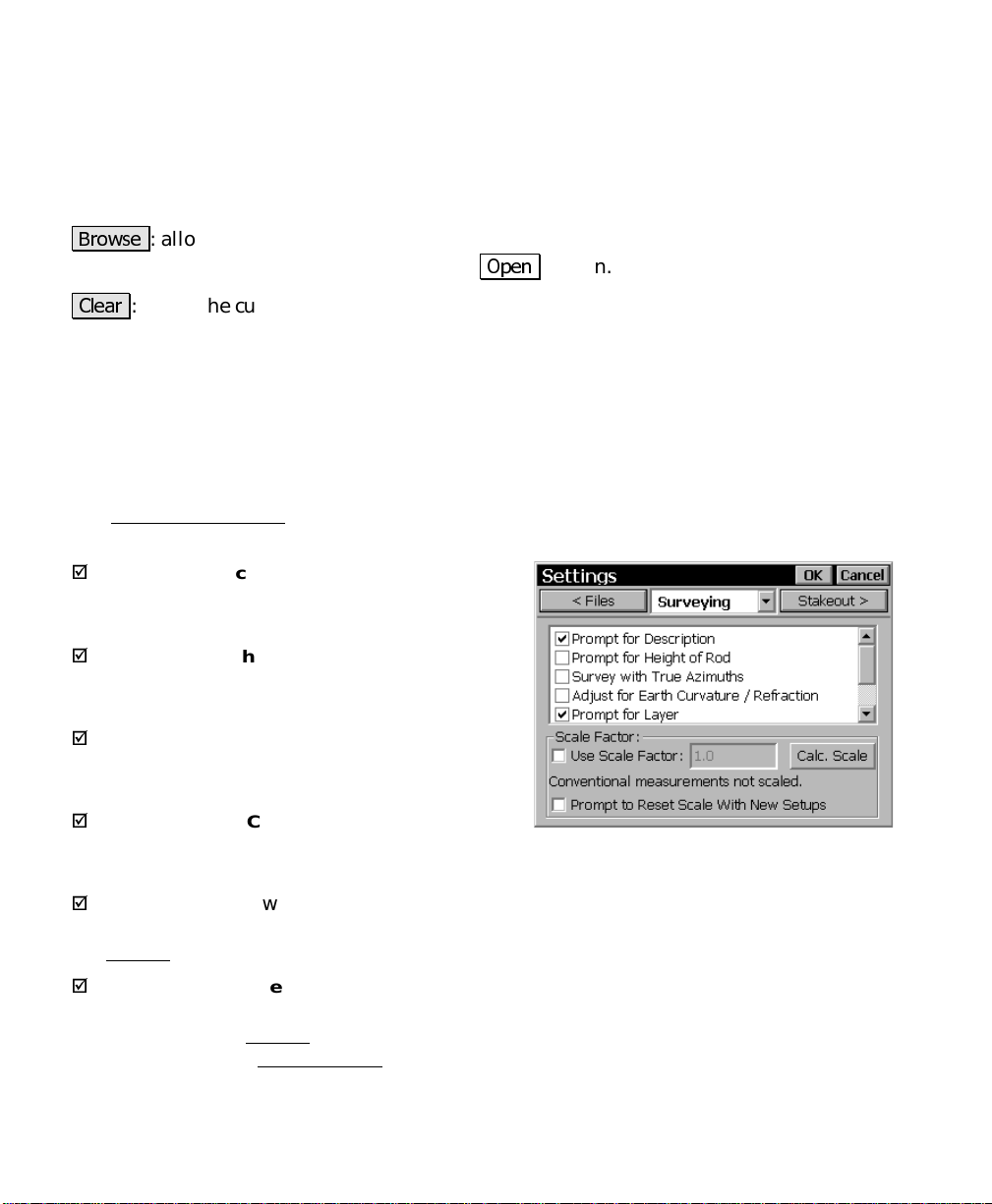
%URZVH

Simply tap on the filename and then tap the

&OHDU

with the current job.

: allows you to select a file to use with the current job.

2SHQ

button.

: closes the currently selected file so that it is no longer used

Surveying Settings

The Surveying Settings allows you to select various options that affect how data collection is performed.

Prompt for Description

;

prompt for a point description will appear before any new point is stored.

Prompt for Height of Rod

;

prompt for the rod height will appear before any new point is stored.

Survey with True Azimuths

;

angle rights will be referenced from true north when traversing.

: when checked, a

: when checked,

Adjust for Earth Curvature / Refraction

;

checked, the elevations for new points are adjusted to compensate for the curvature of the earth and refract ion.

Prompt for Layer

;

appear before any new point is stored from only the routines under the Survey

Prompt for Attributes

;

information will appear before any new point is stored from only the routines under the Survey be selected from the Files Settings

menu.

: when checked, a prompt to select a layer will

: when checked, a prompt to select feature

menu. This also requires that a feature file

card, described above.

: when

Getting Started

Use Scale Factor

;

points will be scaled by the factor entered here. Elevations are not affected.

: when checked, horizontal distances to all new

&DOF 6FDOH

from a selected map projection. If a mapping plane is not already selected, you will fist be prompted to select one.

Prompt to Reset Scale on New Setups

;

projection is selected and you setup over a new location, the specified scale factor is compared to the scale factor defined for your current location in the mapping plane. If the scale factor is different, you will be prompted to use the new scale factor.

: allows you to automatically compute the scale factor

: if checked when a map

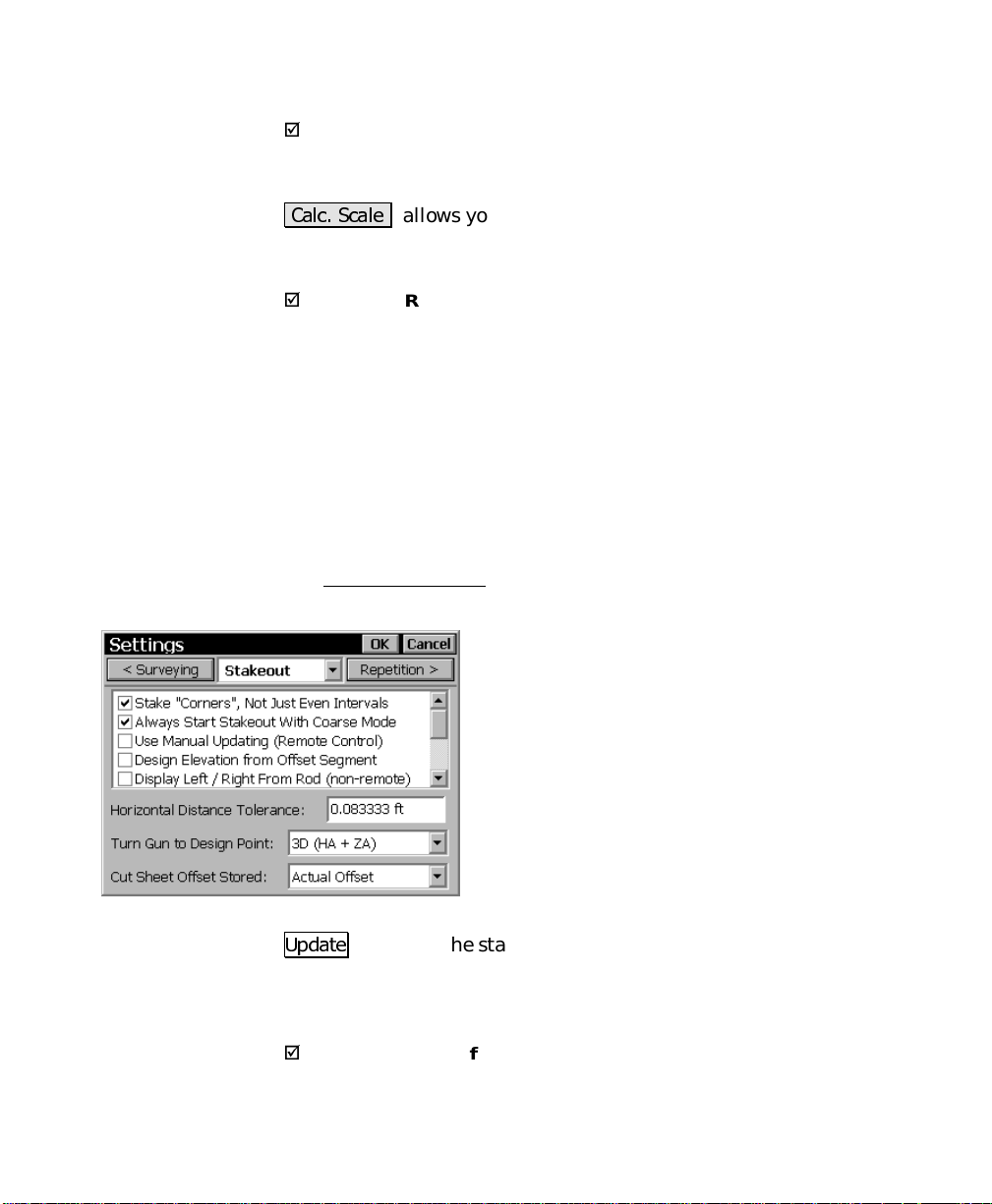
Stakeout Settings

The Stakeout Settings contains the setting that control how stakeout is performed.

Stake “Corners,” Not Just Even Intervals

staking by stations, locations where a line segment changes, such as from a straight section to a curve, will also be staked when this is checked.

Always Start Stakeout With Coarse Mode

when checked, the checkbox found in all stakeout screens will initially be checked. This instructs the total station to measure distances faster, but with slightly less accuracy.

Coarse EDM (fast shot)

: when

Use Manual Updating (Remote Control)

8SGDWH

When this not checked, shots are continuously taken in the stakeout screens. (This is only valid when running in remote mode using a robotic total station.)

;

offset or road stakeout, cut and fill information will be computed from

button in the stakeout screens must be pressed to take a shot.

Design Elevation from Offset Segment

: When this is checked, an

: When checked during

User’s Manual

the design elevation at the node furthest from the centerline of the current segment. When unchecked, cut and fill information will be computed from the design elevation of the segment at the current rod location.

Note: If staking extends beyond the end of th e cross section, the cut / fill information will always be computed from the design elevation at the node furthest from the centerline of the current segment.

Write Cut Sheet Data Only (No Store Point)

;

built points are not stored to the JOB file when staking points; only the raw data is written to the RAW file.

Display Left / Right From Rod (non-remote)

;

move left or right information will be presented from the rod person’s point of view. When unchecked, it will be presented from the total station’s point of view. (This option only applies when a robotic total station is selected in the Instrument Settings

Display Left / Right From Rod (remote)

;

left or right information will be presented from the rod person’s point of view. When unchecked, it will be presented from the total station’s point of view. (This option only applies when a non-robot total station is selected in the Instrument Settings

Prompt for Layer

;

appear before any new point is stored from only the routines under the Stakeout

Prompt for Attributes

;

information will appear before any new point is stored from only the routines under the Stakeout file be selected from the Files Settings

Note: There is no Settings because you will always be prompted for a description when storing a point from a stakeout routine.

menu.

: when checked, a prompt to select a layer will

: when checked, a prompt to select feature

menu. This also requires that a feature

Prompt for Description

card, described earlier.

: When checked, as-

: When checked, the

: When checked, the move

checkbox as in the Survey

Horizontal Distance Tolerance

Staking and Stake to Line routines. When staking to a line and the prism is located at a perpendicular distance to the specified line that

: this setting affects the Remote

Getting Started

is within the range set here, a message will state that you are on the line. When performing Remote Stak eout, the final graphic screen that is displayed when you are near the stake point will occur when you are within the distance to the stake point specified here.

Turn Gun To Design Point

The following options are available:

•

Yes: 2D (HA only)

horizontally toward the design point.

•

Yes: 3D (HA and ZA)

horizontally and vertically toward the design point.

•

Cut Sheet Offset stored

stored to the raw data fi le in either of the following formats when performing any offset staking routine:

•

: The total station must be turned manually.

Design Offset

design-offset values.

Actual Offset

measured-offset values.

: when selected, a cut sheet report will list the

: only applies to motorized total stations.

: The total station will automatically turn

: The cut sheet offset information can be

: when selected, a cut sheet report will list the

User’s Manual

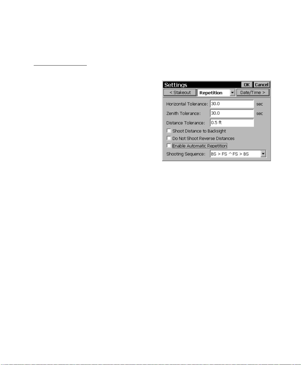
Repetition Settings

The Repetition Settings contains the settings that control how repetition shots are performed and the acceptable tolerances.

Horizontal Tolerance

displayed if a horizontal angle exceeds the tolerance entered here during a repetition shot.

Zenith Tolerance

displayed if a vertical angle exceeds the tolerance entered here during a repetition shot.

Distance Tolerance

displayed if a distance exceeds the tolerance entered here during a repetition shot.

Shoot Distance To Backsight

distance will be measured to each shot to the backsight. When uncheck ed, only the angles are measured.

Do Not Shoot Reverse Distances

measured during reverse shots.

Enable Automatic Repetition

after the first shot to the backsight and foresight will occur automatically when using a motorized instrument.

Shooting Sequence

the following options:

•

BS > FS ^ FS > BS

Backsight

: a warning message will be

: when checked, a

: when checked, distances are not

: when checked, all remaining shots

: specifies the order that the shots are taken from

: Backsight, Foresight, flop, Foresight

•

BS > FS ^ > BS > FS

Foresight

•

BS ^ BS > FS ^ FS

Foresight

•

FS ^ FS > BS ^ BS

Backsight

•

FS > BS ^ BS > FS

Foresight

: Backsight, Foresight, flop, Backsight,

: Backsight, flop, Backsight, Foresight, flop,

: Foresight, flop, Foresight, Backsight, flop,

: Foresight, Backsight, flop, Backsight,

•

FS > BS ^ > FS > BS

Backsight

Getting Started

: Foresight, Backsight, flop, Foresight,

•

BS ^ BS ^ > FS ^ FS ^

Foresight, flop, Foresight, flop

: Backsight, flop, Backsight, flop,

Date/Time Settings

The Date/Time Settings is used to set the date and time in the data collector.

: displays the current date.

Date

: displays the current time.

Time Format

Note: The date, time and UTC are computed using Windows CE’s Date/Time properties.

date that is entered.

: Select

to display Coordinated Universal Time.

UTC

6HW 'DWH

: will set the system date with the

to display your local time,

Local

6HW 7LPH

6\QFKURQL]H

current time and advance to the nearest second so that the time can be set more accurately.

Set DUT

convert UTC to UT1. (UT1=UT C+DUT)

: will set the system time with the time entered.

: when pressed, will zero the fractional portion of the

: is the polar wandering correction factor, in seconds, used to

User’s Manual

General Settings

The General Settings contains the following settings:

Use Enter Key to Move Between Fields

;

when checked, the [Enter] key will move the cursor to the next field in all screens. When unchecked, the [Enter] key will perform a different function depending on the field selected.

Note: The arrow keys and the [Tab] key can also be used to move the cursor between fields.

Allow Alphanumeric Point Names

;

checked alphanumeric point names can be assigned to any point. When unchecked, all point names must be numeri c .

Always Prompt for Backsight Check

;

prompted if you attempt to exit the Backsight Setup first performing a backsight check.

Beep When Storing Points

;

whenever a new point is stored.

Prompt for Description

;

will appear before any new point is stored from any routine other than those included in t he Survey

: when checked, a beep will sound

: when checked, a prompt for a description

and Stakeout menus.

: when

: when checked, you will be

screen without

Prompt for Layer

;

appear before any new point is stored from any routine other than those included in the Survey

Prompt for Attributes

;

information will appear before any new point is stored from any routine other than those included in the Survey This also requires that a feature file be selected from the Files Settings card, described earlier.

Prompt to Backup When Closing Job

;

will open to backup the current job prior to closing it.

: when checked, a prompt to select a layer will

and Stakeout menus.

: when checked, a prompt to select feature

and Stakeout menus.

: when checked, a reminder

Getting Started

Write Point Attributes to Raw Data

;

and attribute information will be written to the raw data file.

: when checked, point feature

Auto time stamp every ___ min

;

record to the raw data file containing the current date and time each time the specified number of minutes passes. This is useful for tracking down when specific raw data records were written to the file.

Remind to backup job every ___ hrs

;

reminder to backup the current job after every specified number of hours passes.

: when checked, will store a note

: when checked, will open a

User’s Manual

Required Files

Every job that is used with TDS Survey Pro actually consists of at least two separate files; a job file and a raw data file. Each file performs a different role within the software.

A job file can be created in the data collector, or on a PC using TDS Survey Link and then transferred to the data collector. A raw data file is automatically generated once the job file is open in the data collector. A raw data file cannot be created using any other method.

There are two other optional types of files that can be used with Survey Pro called control files and description files. Job files and raw data files are explained below. Control files and description files are explained, starting on Page 28 and 32, respectively and include examples to illustrate their use.

Job Files

A job file is a binary file that has a file name that is the same as the job name, followed by a *.JOB extension. A job file is similar to the older TDS-format coordinate file, except in addition to storing point names and their associated coordinates, a job file also contains all of the line work as well.

When you specify points to use for any reason within Survey Pro, the software will read the coordinates for the specified points from the job file. Whenever you store a new point within Survey Pro, the point is added to this file.

A job file can be edited on the data collector when using the Edit Points screen. Since a job file is binary, it requires special software for editing on a PC, such as TDS Survey Link. It can also be converted to or from an ASCII file using Survey Link. (Refer to the Survey Link documentation for this procedure.)

When a job file is converted to an ASCII file, the resulting file is simply a list of points and coordinates. Each line consists of a point name, northing or latitude, easting or longitude, elevation or elliptical height, and a note where each value is separated by a comma.

Getting Started

Raw Data Files

A raw data file is an ASCII text file that is automatically generated whenever a new job is created on the data collector. It has the same file name as the job file (t he job name), followed by the *.RAW extension.

A raw data file is a log of everything that occurred in the field. All activity that can create or modify a point is written to a raw data file. Survey Pro never “reads” from the raw data file – it only writes to the file. Since a raw data file stores all of the activity that takes place in the field, it can be used to regenerate the original job file if the job file was somehow lost. This process requires the TDS Survey Link software.

A raw data file is considered a legal document and editing it can invalidate all of its contents and is not supported in any way by TDS. TDS Survey Link allows you to edit some fields of a raw data file, but other fields cannot be edited since those fields typically tie into other fields in a complex way. Editing these fields in a text editor is possible, but likely to corrupt the contents of t h e raw data file.

When viewing a raw data file on a PC using a simple text editor or on Survey Pro using the View R aw Data unaltered, which can appear somewhat cryptic. When viewing the file from within Survey Link, the codes are automatically translated on the screen to a format that is easier to understand.

screen, the file is shown

Refer to the TDS Web site for a downloadable document that explains the meaning of the codes used in a raw data file.

User’s Manual

Control Files

A Control File is simply an existing job that is optionally opened within the current job so that the points from the control file are also available for use in the current job. The points stored in a control file are called Control Points.

Some users prefer to keep a set of known points in a separate control file when repeatedly working on new jobs in the same general area. That way when they return to the job site, they can create a new job, but select the control file to easily have access to the known control points.

Once a control file is selected in the current job, the control points can be used in the same way as the job’s points with the following exceptions:

• A control file has read only attributes. This means that the points in a control file cannot be modified or deleted; they can only be read. For example, you can select a control point to use as an occupy point during data collection or as a design point during stake out, bu t you could not use a control point for a foresight where you intend to overwrite the existing coordinates with new coordinates. You would also be unable to modify a control point from the Edit Points

screen.

• Since the points in a control file are essentially merged with the points in the current job, you cannot open a control file if any of the point names used in it are also used in the current job. If you attempt to do so, a dialog will tell you that a duplicate point name was encountered and the control file will not be opened.

• Only points are used from a control file. If a control file contains other objects, such as polylines or alignment s, they will be ignored.

Getting Started

Control File Example

The following general example explains one scenario where a control file is used. In this example, a new job is created with a point that has arbitrary coordinates . The control file is selected and used to replace the arbitrary coordinates with coordinates that are in the same coordinate system as those in the control file. The steps in this example can be modified to fit your specific situation.

Assume that you already have a job that contains several known points for an area where you intend to work. You want to create a new job and select the existing job as a control file to make the control points available in the new job. Also, assume that the control file contains points named 1 through 10.

1. Create a new job by selecting Menu.

2. Enter a point name for the first point in the job that will not conflict with the names that are in the control file. In this example, you could enter either any alphanumeric name or any numeric name that is above 10. (Accept the default coordinates for now – they will be overwritten later.)

3. Select the

4. Tap the and select the job that you want to use as a control file.

5. Define your control file and enter the point name that was just created as the

Foresight

6. Take a side s h ot or traverse shot and overwrite the original coordinates with the new coordinates. This will tie in the coordinates for the new point with the coordinates in the control file.

7. Continue your survey.

tab from the Settings

Files

%URZVH

button in the

Occupy

and

)LOH, 2SHQ1HZ

Control File

Backsight

points using points from the

from the Main

screen.

section of the screen

User’s Manual

Description Files

A Description File is used to automate the task of entering descriptions for points that are stored in a job. They are especially useful when the same descriptions are frequently used in the s ame job.

A description file is a text file containing a list of the descriptions that you will want to use with a particular job. The file itself is usually created on a PC, using any ASCII text editor such as Notepad, which is included with Microsoft Windows. It is then saved using any file name and the

It is important to realize that when you use a more sophisticated application, such as a word processor to create a description file, you must be careful how the file is saved. By default, a word processor will store additional non-ASCII data in a file making it incompatible as a description file. However this can be avoided if you use the

Save As…

format as the type of document to save. For more information on creating a text file using a word processor, refer to the your word processor’s documentation.

routine from your word processor and choose a

extension and then transferred to the data collector.

.txt

Text Only

File

Description files can be creat ed in two different formats; one includes codes and the other does not. The chosen format determines how descriptions are entered. Each format is described below.

Description Files Without Codes

A description file that does not contain codes is simply a list of the descriptions that you will want to use in a job. The content of a sample description file, without codes, is shown here.

The following rules apply to des cription files without codes:

• Each line in the file contains a separate description.

• A description can be up to 16 characters in lengt h (including

spaces).

• A description can contain any characters included on a keyboard.

Getting Started

• Descriptions do not need to be arranged in alphabetical order. (Survey Pro does that for you.)

• Descriptions are case sensitive.

To use a description from a description file, simply start typing that description in any

Description

descriptions in the screen.) Once you start typing a description, a dropdown list will appear displaying all of the descriptions in the descriptor file along with all the descriptors that have been used in the current job in alphabetical order. If the first letter(s) that you typed match the first letters of a description in the descriptor file, that

description will automatically be selected in the dropdown list. Once it is selected, you can have that description replace what you have typed by pressing [Enter] on the keypad. You can also use the arrow keys to scroll through the dropdown list to make an alternate selection.

field. (You can experiment with

6XUYH\, 7UDYHUVH  6LGHVKRW

If you wanted file used here, you would have to start typing with lower case characters since descriptions are case sensitive. (Typing not work.)

douglas fir

to be selected with the sample description

… would

Dou

Description Files With Codes

A description file that uses codes is similar to those without codes, except a code precedes each description in the file. A sample description file with codes is shown here.

The following rules apply to des cription files that use codes:

• Each line in a description file begins with a code, followed by a single space, and then the description.

• A description code can consist of up to seven characters with no spaces.

• Description codes are case sensitive.

• The description is limited to 16 characters.

User’s Manual

• Descriptions can include any character included on a keyboard.

To use a description from a description file with codes simply t ype the code associated with the desired description in any As soon as soon as the cursor moves out of the code is replaced with the corresponding description. For example, if you typed lo in a description field while using the description file shown above, lo would be replaced with cursor was moved to another field.

You can combine a description with any other text, or combine two descriptions by using an ampersand (&). For example, entering

Tall&do b&oa

works when spaces are included with the & character. For example, entering

would result in a description of

would have the same result as entering

b&oa

Lodgepole Pine

Tall Douglas Fir

Big Oak Tree

Description

once the

. Entering

. This method also

b & oa

field.

field, the

Note: Remember to check the opening a description file that contains codes, described next.

This File Uses Codes

checkbox when

Opening a Description File

Once a description file is created and stored in the data collector, it is activated with the following steps:

1. Select

2. Select the

File

3. All of the files with a file that you want to use and tap

4. If the description file contains codes, check the

Codes

-RE, 6HWWLQJV

tab and tap the

Files

section of the screen.

checkbox.

from the Main Menu

.txt

%URZVH

extension will be displayed. Select the

button in the

2SHQ

Description

This File Uses

Getting Started

Feature Codes

As explained above, a description or descriptor codes can be used to help describe a point prior to storing it, but this can be a limited solution for describing certain points.

Survey Pro also allows you to describe any object using feature codes. Feature codes can be used to describe objects quickly and in more detail than a standard text description, particul arly when data is collected for several points that fit into the same category. For example, if the locations for all the utility poles in an area were being collected, a single feature code could be used to separately describe the condition of each utility pole.

When describing an object using feature codes, a selection is made from any number of main categories called features. Once a particular feature is selected, any number of descriptions can be made from sub-categories to the selected feature called attributes.

In general, a feature describes what an object is and attributes are used to describe the details of that object.

To take advantage of feature codes, a feature file must first be created using the TDS Survey Attribute Manager, which is included in Version 7.2, or later of the TDS Survey Link software.

The TDS Survey Attrib ute Manager can also be used to view or modify the selected features in a particular job and to export them to any of several different file formats for use in other popular software packages.

Note: You can switch between different feature code files in mid-job, but if a collected attribute does not match an attribute in the current feature code file, it can still be viewed, but not edited.

For more information on creating a feature file, refer to the Survey Attribute Manager section of the Survey Link manual.

User’s Manual

Features

The primary part of a feature code is called a feature. Features generally describe what an object is. Two types of features are used in Survey Pro: points and lines, which are described below.

When assigning a feature to data that was collected in Survey Pro, only features of the same type are available for selection. For example, if selecting a feature to describe a point in a job, only the point features are displayed. Likewise, if selecting a feature to describe a polyline, only the line features in the feature file are displayed.

•

Point Features

A point feature consists of a single independent point. Examples of a point feature would be objects such as a tree, a utility pedestal, or a fire hydrant.

•

Line Features

A line feature consists of two or more points that define a linear object, such as a fence or a waterline. In Survey Pro, these are stored as polylines, but line features can also be used to describe alignments.

Attributes

A feature, by itself, would not be useful in describing a point or line with much detail since a feature only helps describe what the stored point is. Attributes are used to help describe the details of the object.

Attributes are ei ther typed in from the keyboard or selected from a pull-down menu and fall into the following three categories.

•

String Attributes

A string attribute consists of a title and a field where the user can type any characters from the data collector’s keypad up to a specified maximum length. An example of a string attribute is an attribute titled

Notes where the user would type anything to describe a feature.

•

Value Attributes

A value attribute accepts only numbers from the keypad. These attributes are setup to accept numbers that fall in a specified range. Some examples of a numeric attribute would be the height of a tree or a utility pole’s ID number.

Getting Started

•

Menu Attributes

A menu attribute is an attribute that is selected from a pull-down menu rather than typed in from the keypad. Menu items can also have submenu items. For example, you could have a feature labeled Utility with a pull-down menu labeled Type containing Pole and Pedestal. There could also be sub-menu items available that could be used to describe the pole or pedestal in more detail. Menus can only be two levels deep, but there is no limit to the number of items that can be listed in a pulldown menu.

Using Feature Codes in Survey Pro

Before you can use features and attributes to describe points in Survey Pro, you must select a valid feature file to use with the current job.

To select a feature file, open the screen and then select Files Settings. Tap the bottom the appropriate *.FEA feature file.

Once a feature file is selected for the current job, you can configure Survey Pro to prompt for attributes whenever a point, line, or alignment is stored. There are three screens within the

-RE 6HWWLQJV

There is a ;

the Surveying Settings and the General Settings attributes only when an object is stored from the routi n es within the Survey the routines in the Stakeout Settings affects if you are prompted for attribut es when an object is stored from any other routines, such as the COGO

The features and attributes for existing points, polylines, and alignments can also be edited using the Edit Points Polylines and Edit Alignments screens, respectively.

menu. Likewise, the second affects only objects stored from

%URZVH«

. The first affects if you are prompted for

menu. The prompt in the General

button then locate and select

screen to configure this prompt.

Prompt for Attributes

, the Stakeout Settings

-RE, 6HWWLQJV

checkbox in

routines.

and Edit

User’s Manual

Layers

Survey Pro uses layers to help manage the data in a job. Any number of layers can exist in a job and any new objects can be assigned to any particular layer. For example, a common set of points can be stored on one layer and another set can be stored on a different layer.

The visibility of any layer can be toggled on and off, which gives full control over the data that is displayed in a map view. This is useful to reduce clutter in a job that contains several objects. The objects that are stored on a layer include points, polylines, and alignments.

TDS ForeSight can read a JOB file and output an AutoCAD DXF file containing all the original layer information. This conversion can also be performed using TDS Survey Link 7.2, or later via the Survey Attribute Manager, which is included as part of that program.

Layer 0

Layers can be added, deleted and renamed with the exception of

Layer 0

cannot be deleted or renamed.

Layer 0

is a special layer that must exist in every job. It

Layer 0

and is used as a layer for the storage of objects tha t are not assigned to any other layer. Since al l the objects in a job have t o be assigned to a layer, object is stored, but does not exist on any layer.

provides two main functions: compatibility with AutoCAD;

Layer 0

is always there so a situation cannot occur where an

Other Special Layers

Some layers are automatically created, but unlike layers behave exactly the same as any user-created layer; they can be renamed or deleted. Whenever a control file (Page 30) is selected for a job, a control file are stored to that layer. (Any non-point objects in a control file are always ignored.)

Control

layer is automatically created and the points in the

Layer 0

, these

Getting Started

Similarly, whenever a new job is created, a automatically created and selected as the active layer. The active layer is the default layer where any new objects will be stored.

Points

layer is

Managing Layers

You can configure Survey Pro to prompt for a layer whenever an object is stored. If this prompt is turned off, any new objects that are stored will simply be stored to the active layer. There are three

screens within the

-RE 6HWWLQJV

screen to configure this prompt.

There is a ; Stakeout Settings are prompted for a layer only when new data is stored from the routines within the Survey data stored from the routines in the Stakeout the General Settings is stored from any other routines, such as the COGO

Prompt for Layer

and the General Settings. The first affects if you

affects if you are prompted for a layer when data

Most layer management is performed from the

-RE 0DQDJH /D\HUV

you to add, delete, rename and change the visibility of the various layers. You can also set the active layer from here. This screen is also available from several different locations, such as the new Map Display Options the controls that allow you to select layers. The

Ctrl

Manage Layers

checkbox in the Surveying Settings, the

menu. Likewise, the second affects only

menu. The prompt in

routines.

screen. This screen allows

screen and any of

-[K] hotkey can also be used to access the screen.

Changing the Active Layer

To change the active layer, tap the desired layer and then tap the

6HW $FWLYH

can only be one active layer at a time. The active layer is marked with the

button. There must always be an active layer and there

symbol.

User’s Manual

Creating a New Layer

A new layer can be created by tapping Layer dialog box where a name and if the new layer should be visible is entered.

1HZ«

, which opens the New

Changing a Layer Name or Visibility

Selecting a layer and then tapping dialog box where the name and visibility can be changed for the selected layer. You can also edit a layer by double-tapping on it. (

Layer 0

cannot be renamed.)

(GLW«

opens the Edit Layer

Deleting a Layer

You can only delete an empty layer. If a layer contains any objects, they must first be moved to a different layer. To delete a layer, select

the layer and tap

'HOHWH

. (

Layer 0

cannot be deleted.)

Moving Objects from One Layer to Another

The objects on a layer can be moved to a different layer using the object’s appropriate edit screen. For example, to move several points from one layer to another, select t h e desired points in the Edit Points

screen and tap tap 2..

(GLW

. Select the layer you want to move them to and

2D / 3D Points

Survey Pro allows a job to contain 3D points as well as 2D points. Since a 2D point has no elevation associated with it, care should be taken when working with a job that contains any 2D points, especially if you still want to collect 3D points.

If you occupy a point that has no elevation, all the points that are collected from that setup will also have no elevations. Similarly, if you occupy a 2D point and perform stake out, no vertical

Getting Started

data is provided. You can quickly see if there are any 2D points in the current job by

opening the is shown as “

-RE, (GLW 3RLQWV

” is a 2D point.

---

screen. Any point where the elevation

Polylines

Lines can be added to your project that can represent anything such as a roadway, a building, or a lot boundary. These lines are referred to as polylines. Polylines can be compared to the point lists used in other TDS data collection software. They can consist of several individual curved and straight sections. A point must be stored in the project for all the locations on the polyline where a new section begins and ends.

Polylines can be used to compute information such as the perimeter and area for a lot boundary. They can also make it easier to compute and store offset points for the sides of a roadway when a polyline exists that defines a roadway centerline.

Refer to the Reference Manual for information on all the screens that are used to create and edit polylines.

Alignments

Alignments are similar to polylines in that they define specific lines in the current job and typically describe the centerline of a road. An alignment can then be used in the Offset Staking Offset Lines alignments do not need points for the locations where the alignment changes (called nodes).

Alignments are created by separately defining the horizontal and vertical details of a line. Although no points are required to define an alignment, the starting position must be tied to a specific location in the current job, the POB, which can be defined by an exi sting point or known coordinates.

The horizontal and vertical details of an alignment are defined in sections. The first horizontal and vertical section always begins at

, and Slope Staking screens. Unlike polylines,

, Offset Points,

User’s Manual

the specified starting location and each new segment is appended to the previous horizontal or vertical segment.

Once all the horizontal and vertical alignment segments are defined, Survey Pro merges the information to create a single 3-dimensional line.

The vertical alignment (VAL) must be equal in length or greater than the horizontal alignment. The HAL must not be greater than the VAL.

Creating an Alignment

In this step-by-step example, we will create an alignment that has all the possible horizontal and vertical segment types.

1. Select Menu. If any alignments exist in the current job, they will be listed in this screen. An existing alignment can t hen be edited or deleted, but for this example, we will create a new alignment.

2. Tap will open the Edit Alignments screen where you can begin adding horizontal and vertical segments.

3. Tap the

Elev

be the starting location of the horizontal and vertical definition. (Alternatively, you could define the starting location by tapping the



is displayed and then select an existing point.)

-RE, (GLW $OLJQPHQWV

1HZ«

to create a new alignment. This

tab and enter

POB

coordinates of

/RFDWLRQ

/ 3RLQW

from the Main

North, East

5000, 5000, 100

button where 3RLQW

. This will

and

Horizontal Alignment

Getting Started

4. Tap the and then tap the open the Edit Segment screen where the

first horizontal alignment segment can be defined.

5. Tap the segment. Enter a



$]LPXWK

6. Tap 2. at the top of the screen to add the

segment to the horizontal alignment. You will return to the Edit Alignment where the new segment is displ ayed. The graphic shows every horizontal segment entered so far with the selected segment in bold. The dot in the picture indicates the beginning of the selected segment (in this case it is the end). This is where the next segment will be placed when using the

,QVHUW

(Horizontal Alignment) tab

HAL

,QVHUW

button. This will

tab to insert a straight line

Line

Length

of 0.

button.

100

and an

screen

7. Tap the the

8. Enter a 5DGLXV and select a

this segment tangent to previous

that the curve will be positioned so the entrance to the curve is tangent to the end of the previous segment.

9. Tap 2. to add the segment to the horizontal alignment.

,QVHUW

button again and then tap

tab to insert a horizontal curve.

Arc

Right

, a 'HOWD

100

turn. Check the

checkbox so

of 45

Make

User’s Manual

Note: A new segment can be inserted between two existing segments by selecting the existing segment that is to occur after the new

segment and then tapping the

,QVHUW

button.

10. Tap the

Spiral

11. Enter a a and check the

12. Tap 2. to add the segment to the horizontal alignment.

Note: When creating a new horizontal segment and using the

the Edit Alignment screen tagged with a picture). This means that if the previous horizontal segment is edited or deleted, thus changing the orientation, all subsequent horizontal segments that have the also be adjusted so they will remain tangent to the previous segments.

This does not hold true for vertical alignment segments. Vertical segments do not have the and will always begin with the specified starting grade unless they are manually modified.

,QVHUW

button again and then tap the

tab to insert a spiral curve.

Radius

of turn and a

Right

Make this segment tangent to

checkbox.

Make this segment tangent to

option, the new segment will appear in

, a

100

Length CS to ST

Make this segment tangent to previous

200

direction,

(P)

tag will

(P)

, select

(see

option

Getting Started

Vertical Alignment

We have now added all available horizontal segment types. Next, we will define the vertical alignment.

Since the horizontal and vertical alignments are defined independently of each other, the first vertical segment that is defined will start at the same

defined above in Step 3.

POB

Roadway

13. Tap the then tap the

14. Tap the Enter a

15. Tap 2. to add the segment to the vertical alignment.

16. Tap the the

V. Curve

vertical curve. Enter a tap the automatically set the

ending grade of the previous section. Enter an

End Grade

17. Tap

18. Tap the

alignment.

(Vertical Alignment) tab and

VAL

,QVHUW

button.

V. Grade

Length

,QVHUW

*HW 3UHYLRXV *UDGH

to add the segment to the vertical

General

tab to insert a grade.

button again and then tap

tab to insert a parabolic

of -2%.

and a

150

tab and enter a

Grade

Length

Start Grade

button to

of 4%.

250

to the

Description

and

User’s Manual

19. Tap

You have now created a new alignment using all the available types of segments. You can select the new alignment for use in the Offset Staking Offset Points

Note: If the horizontal and vertical alignments end at different stations, they can only be processed in the staking routines as far as the end of the shortest al ignment.

from the Edit Alignment return to the Add/Edit Alignments screen where the new alignment is stored and displayed.

and Offset Lines routines.

screen to

Fieldwork

This section will explain how to get started using Survey Pro to collect data from a total station and perform stake out. It is assumed that you are familiar with the operation of your total station.

The first section describ es the backsight setup procedures for various scenarios. The next section walks you through the steps involved to setup and perform a simple side shot and traverse shot. The third section walks you through a simple point-staking example.

The remainder of the chapter illustrates the procedures to perform the more complex routines in the Survey Pro software in a step-bystep manner. They are intended to explain only how to use a particular routine without the need for you to enter any specific values to read through the example.

When beginning any job, the setup is the same; you need to establish an occupy point and a backsight.

The occupy point is the point where you will setup the total station. The coordinates for the occupy point must exist in the current job or active control file. They can be assumed coordinates; known coordinates; or computed with the resection routine. (Control files and the resection routine are discussed later.) Any point in the current job can be an occupy point.

Once an occupy point is established, the second reference you need is a backsight point or direction. This can be in the form of a point stored in the current job, or an azimuth or bearing.

The horizontal angles recorded during data collection are relative to the backsight. If a point is not available in the job to use as a backsight, you can assume a backsight direction or you can use the solar observation routine, described later, to establish a backsight.

The scenarios below will describe four different possibilities for defining a backsight.

User’s Manual

Scenario One

You know the coordinates and locations for two points on your lot a n d want to occupy one and use the other as a backsight.

Solution

1. Create a job using the coordinates for one of the known points as the first point.

2. Use the Edit Points coordinates for the remaining known point.

3. From the Backsight Setup point number of one known point and setu p the total station over that point.

4. Toggle the enter the point name for the second known point in that field.

20. Aim the total station toward the other point, zero the horizontal angle on the instrument, and tap

Always Prompt for Backsight Check Settings

backsight.

You are now ready to start your survey.

%6 'LUHFWLRQ

General

routine to add a second point using the

screen, set the

%6 3RLQW

6ROYH

option is checked in the

screen, you will be prompted to check your

Occupy Point

button to

, then

%6 3RLQW

&ORVH

field to the

and

. If the

Job

Scenario Two

You have found two points on your lot and know the azimuth between them, but you do not have coordinates for either.

Solution

1. Create a job using the default coordinates for the first point.

2. From the Backsight Setup point that was just created.

3. Setup the total station over the point where the known azimuth is referenced.

screen, set the

Occupy Point

field to the

Fieldwork

4. Toggle the enter the known azimuth to the second point here.

5. Aim the total station toward the second point, zero the horizontal angle on the instrument, and tap

You are now ready to start your survey.

%6 'LUHFWLRQ

%6 3RLQW

button to

6ROYH

, then

%6 'LUHFWLRQ

&ORVH

and

You may want to take a side shot from the Traverse Sideshot to the backsight point so that you have coordinates for it. The horizontal angle would remain at zero during this shot.

If you later find true State Plane coordinates for any of the points in your job, you can use the Translate coordinates accordingly.

routine to adjust all the

screen

Scenario Three

You have one point establi shed on your lot and you know the azimuth to an observable reference.

Solution

1. Create a job using the coordinates of the established point for the first point. If the coordinates are unknown, accept the default coordinates.

2. From the Backsight Setup point that was just created.

3. Setup the total station over the established point.

4. Toggle the enter the azimuth to the observable reference here.

%6 'LUHFWLRQ

screen, set the

%6 3RLQW

button to

Occupy Point

%6 'LUHFWLRQ

field to the

and

5. Aim the total station toward the observable reference, zero the horizontal angle on the instrument, and tap If the

Always Prompt for Backsight Check

Job

Settings

your backsight.

If you later find true State Plane coordinates for any of the points in your job, you can use the Translate coordinates accordingly.

General

screen, you will be prompted to check

routine to adjust all the

6ROYH

, then

option is checked in the

&ORVH

User’s Manual

Scenario Four

You have only one known point on a job.

Solution

You have two options in this situation. One, you can assume an azimuth for an arbitrary backsight reference and rotate the job later using the Rotate orientation.

routine once you have determined the actual

Secondly, you can use the Sun Shot to an arbitrary reference.

routine to determine an azimuth

Summary

In general, you would follow these steps when you begin working on a job.

1. Create a new job or open an existing job.

2. Setup over the

3. Aim the total station toward the backsight and zero the horizontal angle on the instrument.

4. Fill in the Backsight Setup the

Always Prompt for Backsight Check

Job

Settings

your backsight.

5. Start your survey.

Note: You should enter the correct

Backsight

your backsight using the Check by Distance routine.

distances in the Backsight Setup

Occupy Point

General

screen and tap

screen, you will be prompted to check

Height of Instrument

6ROYH

, then

option is checked in the

screen if you plan to check

and

&ORVH

Height of

. If

Fieldwork

Note: If the displayed is subtracted from all horizontal angles that are read during data collection and the resulting points are adjusted accordingly. This will happen after survey with true azimuths or performing stakeout in a special mode. If you do not want this to happen, you should change this value to zero from the Backsight

Circle dialog box by tapping the

Most non-staking related data collection is performed from the Traverse / Sideshot button, the routine expects that you will eventually be occupying the

foresight that you are shooting and backsighting your current occupy point. When you are ready to setup on the next point, the occupy, foresight and backsight points will automatically be updated accordingly.

After taking a shot using the expect the total station to be moved before the next shot and will therefore only automatically advance the foresight point.

Backsight Circle

screen. When you take a shot using the

displays a non-zero value, the angle

%DFNVLJKW &LUFOH button.

7UDYHUVH

6LGH 6KRW

button, the routine does not

Data Collection Example

This section illustrates the necessary setup and usage of the Traverse / Side Shot screen, which is the primary screen used during data collection. We will create a new job and manually add another point to the job to use as a backsight. We will run in manual mode so the shot data must be entered manually. This example, and the following stakeout example a re the only examples that are designed where the user should follow along and enter the values in their data collector as they are provided in the example.

User’s Manual

Setup

1. Create a new job. a. From the Main Menu

2SHQ  1HZ

b. Tap

c. Enter any job name that you wish in the

d. For this example, simply accept the

1HZ«

Job screen

Job Name

default job settings and tap

to open the Create a New

field and tap

, select

1H[W !

)LOH

1H[W !

Fieldwork

Note: When creating a new job, it is important that the

Distances

seamlessly swit ch between different units in mid-job. Problems can arise i f these units are inadvertently set to the incorrect

units prior to entering new data. For example, assume you created a control file by hand-entering a list of coordinates in a new job where the job was set to Now assume you created another new job and correctly set it to

Survey Feet

the new job, the display of all of the coordinates in the control file would be converted from Feet to US Survey Feet.

field be set to the correct units. This allows you to

and the coordinates were in

Feet

. If you then selected the previous job as a control file for

e. Accept the default coordinates for the

first job point by tapping

2. Check the Job Settings. a. Tap

b. Tap the

c. For this example, tap the

-RE, 6HWWLQJV

Menu to open the Settings screen.

Instrument

both the to

Settings

Brand

Manual Mode

and un-check all the checkboxes.

from the Main

tab and make sure

and

Model

Units for

US Survey Feet

)LQLVK

fields are set

Surveying

d. Tap 2. to save the job settings.

3. Add a backsight point to the job. a. Select

-RE, (GLW 3RLQWV

from the Main Menu.

User’s Manual

b. Tap

,QVHUW«

using the with the following values, as shown:

Point Name Northing Easting Elevation Description

and then tap 2..

and enter a new point

General

5050

100

and

Backsight

Location

cards

4. Set up your backsight. In this example, we will set up on Point 1 and backsight Point 2, which was just created.

a. Access the b. In the

Tip: You can also select an existing point from a map view or from a list by using the power button.

c. Enter an HI and HR of 5 feet each. d. Toggle the

%6 3RLQW

e. Leave the f. Confirm that the

non-zero value, tap the

6XUYH\, %DFNVLJKW 6HWXS

Occupy Point

%6 'LUHFWLRQ

and enter 2 as the point name.

Fixed HR at Backsight

field, enter 1 as the point name.

%6 3RLQW

field unchecked.

Backsight Circle

&LUFOH«

value is zero. If it displays a

button and set it to zero.

screen.

button to

g. Tap

6ROYH

. The Map

Fieldwork

screen will open automatically.

h. Tap

&ORVH

to continue.

Performing a Side Shot

5. Access the appropriate fields. The backsight information is displayed at the top of the screen. At this point, it is assumed that your total station is over the occupy poin t and its horizontal angle was zeroed while aiming toward the backsight.

6LGH 6KRW

compute coordinates for the new point and store it. Since we are running in manual mode, we will enter the shot data from the keypad.

6XUYH\, 7UDYHUVH  6LGHVKRW

a. In the Traverse / Sideshot

the following data:

Foresight Description HR

These values will define the point name, description, and rod height for the next point that is stored.

b. Assuming that the total station is

aiming toward the prism, which is located over the foresight, tap

. This would trigger the total station to take a shot,

: 3

: 5

screen and fill in the

screen, enter

c. Enter the following data:

: 90

: 70

100

. The new point is

Foresight

point

Angle Right Zenith Slope Dist

and then tap computed and stored. The

will automatically advance to the next available point name and the information from the last shot is displayed on the screen.

User’s Manual

d. You can see a graphical representation of

the previous shot, as shown here, by tapping the more information on the Map View

tab. See Page 14 for

Map

Performing a Traverse Shot

6. The steps involved in performing a traverse shot are nearly identical to performing a side shot. The difference is you must specify if you plan to move the total station to the current foresight point after the shot is taken.

a. Tap the

point should now be updated to 4.

b. Assuming that you are now aiming the total station at a

prism located over the foresight point, tap would trigger the total station to take a shot, compute coordinates for the new point and store it. Since we are running in manual mode, we will enter the shot data from the keypad.

c. Enter the following data:

Angle Right Zenith Slope Dist

and then tap

: 90

,QSXW

tab of the Traverse / Sideshot.

: 45

: 50

The Foresight

7UDYHUVH

. This

Fieldwork

d. The new point is computed and

stored and the Traverse Now or Later prompt will open, shown here, asking if you want to advance to the new point now or later. For this

example, tap the button. The New Occupy Point

dialog box will open, shown here, which displays details of the new setup. You can see that the previous foresight point is now the current occupy point and the previous occupy point is now the current backsight point.

e. Since we are running in manual

mode and cannot send data to an instrument, tap notice at the top of the Traverse

Sideshot screen that the occupy point

has been updated to 4, the backsight is updated to 1, and the foresight is updated to 5, which is the next available point name.

7UDYHUVH 1RZ

&ORVH

. You will

Note: If you select to traverse later, the traverse point is still stored, but you will then have the opportunity to shoot additional side shots before you advance to the next point. This is useful when you want to shoot the traverse shot first, before any settling occurs to the tripod. In that situation, when you are ready to advance, you would tap

7UDYHUVH

you are ready to advance or re-shoot the traverse point. (If you select to re-shoot the traverse poin t, the previous traverse point is stored as a side shot.)

When out in the field, you would now move your total station over the new occupy point, aim it toward the previous occupy point (the current backsight), enter the correct instrument height in the

of Instrument

update the Traverse / Side Shot screen and set the total station’s

again where you would then answer to a prompt that asks if

Height

field and tap

6HQG &LUFOH WR ,QVWUXPHQW

. This would

User’s Manual

horizontal angle to zero where you are then ready to collect more data.

You have now created a job, checked the settings, setup a backsight and collected data in the form of a side shot and a traverse shot. If at any time you want to view the coordinates of your points, you can do

so from the

-RE, (GLW 3RLQWV

screen.

Data Collection Summary

1. Open or create a job.

2. Check the job settings.

3. Setup a backsight.

4. Collect data in the form of traverse shots or side shots.

Fieldwork

Stakeout Example

When setting up to perform stakeout, the requirements a re nearly the same as with data collection. You need an existing occupy point, backsight point or direction, and a foresight. The main difference is existing points are being located during stakeout rather than new points being collected.

In the example below, all of th e steps required to perform a simple point-staking job are explained from the initial setup to the staking itself. For consistency, this example assumes you are running Survey Pro in manual mode so the shot data will need to be input from the keypad. Since the software behaves differently in manual mode compared to when using a total station, the differences ar e noted where applicable.

For this example we will use the job that was created with the Traverse / Side Shot Example, above. When staking the first point, we will take two shots to the prism to “home-in” on the design point. When staking the second point, we will only take one shot combined with the Store/Tape

routine to store the stake point.

User’s Manual

Set Up

1. Open the job that was created in the Traverse / Side Shot Example if it is not already open.

a. From the Main Menu

Open / New screen.

b. Tap the file name that was created

earlier listed in the and then tap that job are shown here.

2. Set the job settings. (Only the settings that affect this example are covered here.)

a. Select

Menu.

b. Select the

set both the

Manual Mode

c. Select the

the checkboxes are unchecked.

d. Select the

Sheet Offset Stored

Actual Offset

Note: When performing stakeout, you have t h e option of storing cut sheet information. This information is stored in the raw data file, and when using software on a PC, such as Survey Link, it can be extracted in the form of a Cut Sheet Report.

2SHQ

-RE, 6HWWLQJV

Instrument Settings

Brand

Surveying Settings

Stakeout Settings

, select

Open Recent Job

. The coordinates for

from the Main

and

Model

field (at the bottom of the screen) is set to

)LOH, 2SHQ  1HZ

list

screen and fields to

screen and confirm that all of

screen and make sure the

to open the

Cut

e. Tap 2. to save the job settings.

3. Setup your backsight. In this example, we will setup on Point 1 and backsight an object with a known azimuth. When connected to a total station, you would setup over your occupy point, aim toward the backsight and zero the horizontal angle in the total station before continuing.

a. Access the

screen from the Main Menu.

6XUYH\, %DFNVLJKW 6HWXS

Fieldwork

b. In the

point name.

c. Toggle the

button to

the backsight azimuth. d. Enter an HI and HR of 5 feet. e. Leave the

unchecked.

f. Confirm that the

non-zero value, tap the zero.

g. Tap

6ROYH

representation of the occupy point and backsight direction. Tap

&ORVH

Backsight Circle

. A map view will open that shows a graphical

to continue.

Occupy Point

%6 'LUHFWLRQ

Fixed HR at Backsight

%DFNVLJKW &LUFOH

Staking Points

4. Stake the first design point (Point 2). a. Access the

6WDNHRXW, 6WDNH 3RLQWV

information is displayed near the bottom of the screen. At this point, it is assumed that your total station is over the occupy point and its horizont al angle was zeroed while aiming toward the backsight.

field, enter 1 as the

%6 'LUHFWLRQ

value is zero. If it displays a

screen. The backsight

%6 3RLQW

and enter 0 as

button and set it to

field

b. Enter the following data in the Stake

Points screen:

Design point Increment Height of rod

and tap

: 5

6ROYH !

User’s Manual

c. The second Stake Points

that displays all of the information needed to locate the design point. When connected to a total station, you would turn the total station horizontally to 45°00’00”, vertically to 90°00’00” and send the rod man out about 70 feet before

continuing. Tap the continue to the third screen.

screen will open

6WDNH !

button to

d. With a

button. (See the Reference Manual for an explanation of the other fields.)

e. Enter the following shot data:

Angle Right Zenith: 90 Slope Dist

and then tap

f. The Stake Points screen will show the

necessary

Go LEFT

must move in order to be located over the design point. In this example, the Go the rod is precisely on the line between the total station and the design point. The indicates that the rod must move back (away from the total station) 0.711 feet to be over the design point. The zero so no dirt needs to be cut or filled at the rod location to match the design elevation.

g. Assuming the rod has been repositioned, take another shot by

tapping the data:

Angle Right Zenith Angle Slope Dist

and then tap

Height of rod

: 45

: 70

COME

information that the rod man

6KRW

: 45

: 90

70.8

of 5, tap the

to continue.

/ GO and Go

RIGHT

BACK

button and enter the following new shot

to continue.

6KRW

RIGHT

value indicates 0, which means value indicates

0.711

, which

value is

Fill

h. According to the screen, the rod must

now move over the design point. We will assume that this is close enough and will store the point from this shot by tapping the

6WRUH«

i. Enter the following point information:

Point Name Description

and tap the first Stake Points screen.

5. Stake the next design point. a. We want to stake the next design point

in the project. We can do this by entering 3 in the

then pressing simply tap

automatically advance the current design point by the increment value and solve automatically. Either method will send you to the second Stake Points screen.

FORWARD

button.

Staked

6WRUH

1H[W 3RLQW !

. This will return you to

6ROYH !

0.089

Design Point

, or we can

, which will

field and

Fieldwork

feet to be

Note: A negative next design point to count down when tapping

b. The information needed to locate the next design point is

displayed. When connected to a total station, you would turn the total station horizontally to 115°00’00”, vertically to 90°00’00” and send the rod man out about 100 feet before

continuing. Tap the screen.

c. Tap the

Angle Right Zenith Slope Dist

and then tap

6KRW

: 90

Increment

115

99.8

value results in the point number for the

1H[W 3RLQW !

6WDNH !

button and enter the following shot data:

to continue.

button to continue to the third

User’s Manual

d. The rod man needs to move back by 0.2

feet to be over the design point. Rather than take another shot, we will instruct him to use a tape and place a stake at

that location. Tap the button to store the point.

e. Enter the following data in the Store

Point (Tape Offset) Dialog Box:

Point Name Description Tape Out/Tape In (+/-)

and tap point that are 0.2 feet further from the total station than the last shot to the prism.

: 6

Staked

6WRUH

. This will result in coordinates for the stored

6WRUH7DSH«

0.2

Note: The default value in the directly over the design point, assuming you are on line.

Note: Negative and positive values are away from the total station.

Tape Out/Tape In

values are toward the total station

field should put you

Point Staking Summary

1. Open a job that contains the design points that you want to stake.

2. Check the job settings.

3. Setup a backsight.

4. Stake the points from the Stake Points

screen.

Fieldwork

Surveying with True Azimuths

Some people need to collect all of thei r horizontal angles in the form of azimuths. Survey Pro CE can help automate this process by computing the backsight azimuth after each new setup in a traverse and updating the backsight circle and total station’s horizontal angle accordingly.

1. You can setup on any existing point and use any other point in the job as a backsight if the coordinate syst em is properly aligned with true north. If not, you can occupy any point as long you have a known azimuth to any reference.

2. In the Surveying Settings confirm that the

3. Setup the total station over the occupy point and aim it toward your backsight.

4. Access the Backsight Setup toggle the

Note: When backsighting on a point, selecting be used, as described next, making it easier to view the azimuth to the backsight.

5. If backsighting a known azimuth, enter it in the field. If backsighting a point, use the shortcut method to enter the azimuth from the occupy point to the backsight point in the

BS Direction

backsighting Point 2, enter cursor leaves that field, the computed azimuth will replace what you typed.

6. Tap the

Backsight Circle

running in Manual Mode). This will set the backsight circle as the horizontal angle in the total station and set the same angle as the from all horizontal angles sent from the total station.

&LUFOH«

Backsight Circle

Survey with True Azimuths

%6 'LUHFWLRQ

field. For example, if you are occupyin g Point 1 and

button, enter the backsight azimuth in the

field and tap

value. This angle will then be subtracted

screen (

screen; enter the

%6 3RLQW

1-2

-RE

button to

in the

6HQG WR ,QVWUXPHQW

6XUYH\LQJ

checkbox is checked.

Occupy Point

%6 'LUHFWLRQ

BS Direction

%6 'LUHFWLRQ

BS Direction

field. Once the

(or

6HWWLQJV

, and

can still

6HW

when

User’s Manual

7. Begin your survey. When you traverse to a new point, the New Occupy Point will open showing you the azimuth computed to the new backsight point from the new occupy point. Once you are setup over the new occupy point, and aiming toward the new backsight point, press the

6HQG &LUFOH WR ,QVWUXPHQW

the

Backsight Circle

angle on the total station. Repeat this step after setting up on each new traverse point.

value and the horizontal

button to update

dialog box

Road Layout

Overview

The Road Menu contains a powerful set of routines that allow you to enter and modify road layout information and then stake the road in the field. The road staking routines allow you to stake any part of the road or slope stake th e road.

There are four basic components of a road: The Horizontal Alignment; the Vertical Alignment; Templates, and a POB. All of these components are described separately below and each is a required component to a complete road definition.

Horizontal Alignment (HAL)

The horizontal alignment, referred to as the HAL, defines the horizontal features of an alignment. It can contain information on straight, curved, and spiral sections of the alignment. Generally the HAL coincides with the centerline of a road, but it is not required to be the centerline. All stationing for an alignment will come from the HAL.

Vertical Alignment (VAL)

The vertical alignment, referred to as the VAL, defines the vertical components of the alignment including grades and parabolic vertical curves.

The VAL is generated in the same way as the HAL. The VAL can be the same length as the HAL, or longer, but it cannot be shorter.

Templates

Templates contain the cross section information for the road. Templates are stored in separate files with a TP5 extension so they can be used with multiple job s. The templates are broken down into

User’s Manual

sections, called segments. Each segment contains a specified length, and slope or change in elevation. Templates can contain as many segments as needed, but must have at least one segment. Each segment describes one component of the cross section such as the roadbed, curb face, top of curb, ditch, etc. Each road alignment can contain as many templates as required to define the roadway, but all the templates used on one side of the road must have the sa me number of segments.

Templates can be further modified using widenings and super elevations:

Widenings are used to widen or to narrow the first segment of a template. The remaining segments of the template are not affected. This feature is intended to be a way of controlling the width of the first segment, typically the roadbed, without having to create and manage additional template files. Widening definitions basically act as two templates that modify the first segment.

Super elevations are used to bank curves in the direction of a turn. A super elevation accomplishes this by changing the slope of the first segment of a template – the slope of any remaining segments will remain unadjusted.

One super elevation defines a begin station and an end station where the slope change begins and where it finishes the transition for one side of a road. Therefore, to ba n k a two-lane road, four super elevations would be required – one at the beginning and one at the end of the curve for each side of the road.

A super elevation can either hinge at the outer edge of the first segment, or at the centerline. Hinging at the center results in the elevation of the outer segments to change. Hinging at the edge results in the elevation of the centerline changing. Because of this, Survey Pro will only allow you to hinge on edge for one side of a road. If the other side is also super elevated, you will be forced to hinge that side at the center so that an abrupt change in elevation does not occur at the centerline.

Road Layout

POB

The POB designates the location in the current job where the alignment starts. The POB can be defined by an existing point or specified coordinates and can be changed at any time. The VAL’s start station elevation will be set from the POP.

Road Component Rules

The following section defines how the various components described above work together to form the road. This information is important because how each component reacts to the other component affects the shape of the resulting road.

Alignments

1. The alignment must have both HAL and VAL segments.

2. The VAL must be eq ual to, or longer than the HAL .

Templates

1. For each side of the road

• All templates on a particular side of the road must have the same number of segments for. The fist template for each side of the road defines this number.

• The station for the first template for each side must match the starting station of alignment.

• All template stations must be within the station range for the alignment.

• All templates must have at least one segment.

• A template can contain one zero length segment making it

effectively a blank template, but the first segment must be greater than 0.

• Template segments must have a name. The template editor provides fields to enter the segment name.

User’s Manual

2. Any two templates without intervening Widening or Super Elevations will transition.

• This means that each template segment will transition at a

linear rate from its existing offset from the centerline to the new offset from the centerline as defined by the new template.

3. A template’s first segment slope and/or width will be modified when:

• A template is located within a Super Elevation or Widening

definition including starting and ending stations and inside Widening or Super Elevation transition areas.

• Templates will acquire first segment slope value from the

Super Elevation definition, and/or acquire its first segment width value from the Widening definition.

4. Only one template may occupy any station.

• As little as 0.001 units can be used to separate templates.

Widenings and Super Elevations.

1. Super Elevation and Widening stations must be within the station range of the alignment.

2. Super Elevations and Widenings follow the same rules except that the start and end stations of a Super Elevation are defined by:

• Super Elevations will start their transitions at a point equal

to the user defined starting station minus ½ of the starting parabolic transition length if parabolic transitions are used.

• Super Elevations will start their transitions at a point equal

the user defined ending station plus ½ of the ending parabolic transition length if parabolic transitions are used.

3. Super Elevation start slope value and Widening start width value must match the first segment value defined by:

• A previous Super Elevation or Widening. (Priority)

• A previous Template.

Road Layout

4. Super Elevation ending slope value and Widening ending width value must match the first segment value defined by:

• A following Super Elevation or Widening. (Priority)

• A following Template.

• Exception: if the Widening or Super Elevation is the last

element in the road, it’s end transition value does not have to match anything.

5. Super Elevation and Widening ending stations must be greater than their beginning stations.

6. Widenings cannot adjust the first segment horizontal distance to or from 0.

7. Super Elevations and a Widenings may overlap, are independent, and do not affect each other.

8. Super Elevations may not overlap other Super Elevations.

• A Super Elevation’s ending station may be equal to a

following Super Elevation’s beginning station.

• A Super Elevation’s beginning station may be equal to a

previous Super Elevation’s ending station.

9. Widenings may not overlap Widenings.

• A Widenings ending station may be equal to a following

Widening’s beginning station.

• A Widening’s beginning station may be equal to a previous

Widening’s ending station.

10. Super Elevations may hinge on edge.

• Hinge on edge can only be used for one side of the road for

any given Super Elevation station range.

• If hinge on edge is used for one side of the road, Super

Elevations must hinge from center on the opposite side of the road over the same station range.

• Hinge on edge will modify the elevation of the Center Line.

User’s Manual

Road Rules Examples

Figure 1 Overhead view of a template-to-template linear transition

Figure 2 Template to Widening Transition

Road Layout

Figure 3 Widening to Template Transition

Figure 4 Widening to Widening Transition

User’s Manual

Figure 5 Template Inserted Into A Widening Area

Figure Descriptions

Figure 1 shows an overhead view of a simple transiti on from one template to another. Notice the linear transition of one template segment end node to the next.

Figure 2 shows an overhead view of a basic template to widening transition. The widening’s first segment width for the start station must match the first segment width of the previous template.

Figure 3 shows a transition from a widening to a template. This example shows that a widening basically defines a new template that has a modified first segment. The modified template (widening) will transition to the next template down the road.

Figure 4 shows the same concept as Figure 3 except another widening is used instead of a template.

Figure 5 depicts how a template can be inserted inside a widening definition. The widening will take precedence over the first segment so the first segment will maintain the length as defined in the widening definition. However, the segments outside of the first segment now take on the shape of the inserted template. Th e figure shows a widening where the start width is the same as the end width but having the widening use the same start and end width is not required. The first segment of the template will be adjusted to match

Road Layout

whatever the widening says the width of the first segment should be at the station where the template is inserted.

Also notice in Figure 5 that we have defined a widening with the start width the same as the end widt h. This can be a handy tool to use if you need to widen the road for a relatively long distance but also need to change the template segments outside the first segment. Using a widening as shown enables you to use any template to modify the outside segments while retaining the same roadbed (first segment) width.

Super Elevations

The examples above show how widenings interact with templates. Super elevations work with templates in the same way, except instead of the width of the first segment being modified, the cross slope for the first segment is modified.

Creating Templates

The information for a single template is stored in a separate file with a TP5 extension. Template names are limited to eight characters plus the extension so that they can be used in DOS-based data collectors. Each template stores information on the cross section for one side of the road.

A road can have as many templates as necessary, but each side of the road must only use templates with the same number of segments. Once the first template is selected, Survey Pro will only let you select from additional templates that have the same number of segments as the first template.

A template can be used on either side of the road. They are not right or left specific. A road could contain only one template, which would be used for both the right and left sides, but can also contain as many templates as necessary.

In this example, we will create a single template that contains a roadbed, a curb, and a ditch. Each segment will be defined in order, starting from the centerline and working toward the edge.

User’s Manual

1. Tap

5RDGV, (GLW 7HPSODWHV

screen.

to open the Add/Edit Templates

2. Tap and

1HZ«

Fill Slope

to open the New Template

screen. The

values are the slopes to compute the location of

catch points with the Road Slope Staking

routine. These

values can also be easily changed from that routine.

3. Tap

,QVHUW«

. This will open the Edit Segment dialog box. Enter the following information to define the first segment, which will be a 20-foot wide roadbed with a -2% slope.

Segment Name:

Roadbed

Horizontal Distance: 20 Slope:

4. Tap 2. to return to the New Template

-2

screen where the new roadbed segment will appear. A list of segments is displayed. At this point, only the roadbed and

will be displayed in

<End>

the list. Whenever a new template it inserted, it is inserted above the template that is selected in this list. Therefore, to add a new segment to the end of the last segment,

selected prior to tapping

<End>

,QVHUW«

should be

Cut Slope

5. With

<End>

selected, tap

,QVHUW«

and enter the following data to add a new segment that will describe the face of a curb. Notice for the last field, you need to toggle the 6ORSH

button to 9 2IIVHW

and select the

radio

button to specify that the curb extends upward.

Segment Name:

Curb

Horizontal Distance: 0 Vert Dist:

U 0.5

6. Tap 2. to return to the New Template curb segment will appear.

Road Layout

screen where the new

7. With

<End>

Segment Name: H. Offset: 2 Slope:

-40

selected, tap

8. With

Ditch

,QVHUW«

data to add a sidewalk and then tap 2..

Segment Name: Horizontal Dist: 4 Slope:

enter the following data to add a ditch and then tap 2..

<End>

9. Tap 2. from the New Template screen and the Save As dialog box will open. Enter T1 in the and tap 2.. This completes the creation of a template.

and enter the following

Sidewalk

selected, tap

,QVHUW«

and

Name

field

Building an Alignment

The Edit Alignments routine is used to create an alignment and is explained in detail starting on Page 41. If you do not currently have any alignments stored on th e data collector, either create a simple alignment now that is at least 300 feet long, or follow the instructions that start on Page 41 to create a new alignment that contains each possible type of horizontal and vertical section.

User’s Manual

Putting the Road Together

The final step in creating a road that can be point staked or slope staked is to use the Add/Edit Roads template(s) with the alignment and define any widenings and super elevations.

In this example, we will use only one template for the entire road. We will use a widening to add a second lane to the right side of the road and we will add four super elevation definitions to bank the left and right side of a curve.

Add Templates to the Alignment

routine to combine the

1. Tap

2. Since we are creating a new road, tap

3. With the

4. Tap the

5. Tap the

5RDGV (GLW 5RDGV

to open the New Road screen.

5RDG

tab selected, enter a name for the road in the example, we used

&KRRVH $OLJQPHQW«

select an alignment. In this example, we selected the

Page 41. Tap 2. to continue.

6HW 32%«

Alignment Properties screen to define where the road begins in the job.

Road Name

Roadway

to open the Add/Edit Roads screen.

1HZ«

field. In this

Example

to open the Road

button and

alignment created on

Road Layout

6. Enter the following data then tap 2.:

5000

North: East: Elev: Start Station:

5000

100

0+00

7. The next step is to add the templates. We will use the template created earlier to define both sides of the road. Tap the

7HPSODWHV

tab.

tap the

8. With

$GG«

button. This opens the Add Left Template

selected in the Left column,

<End>

screen,

which allows you to add a template to the left side of the road.

9. All the available templates will be displayed in the

Template

column. Select the T1 template, created earlier.

10. Since we will use this template for both sides of the road, check the

checkbox and tap 2.. We now

Right

;

Mirror to

have the minimum number of components to completely define a road: an alignment, and a left and right template.

11. Tap

&KHFN«

to confirm that the road is okay. You should get a message stating success.

Note: once templates have been added, you can return to the Road card and tap the

9LHZ 3URILOHV«

button to view the cross-sectional

profile of the road at any station.

User’s Manual

Add Widenings

12. Tap the lane will begin in the right side of the road.

13. Tap the Widening screen, which allows you to add a

widening to the right side of the road

14. In the Start Station field, enter 0+25. This is where the widening will begin.

15. The length of the widening is 100 feet so toggle the (QG 6WDWLRQ and enter

16. The starting width of a widening must equal the width of the first segment of the template that leads into the widening, or if a previous widening leads into it, it must equal the width of the previous widening. Leave the value of 20.

17. Since we are adding a lane with this widening, enter 40 in the

Ending Width

over a 100-foot span; the first segment of the template will increase in width from 20 feet to 40 feet. Bold lines in the map view illustrate the beginning and ending widths of the widening.

:LGHQLQJV

in the Right column and then tap

<End>

$GG«

button. This opens the Add Right

100

tab. We will define a widening where a new

button to /HQJWK

Starting Width

field. This widening will now begin at 0+25 and

field set to its default

18. Tap 2. to continue.

Add Super Elevations

19. Tap the elevation at the beginning and end of a curve for the left and right sides of the road.

20. With This opens the Add Left Super Elevation screen, which allows you to add a super elevation to the left side of the road.

6XSHU (OHYDWLRQV

selected in the Left column, tap the

<End>

tab where we will insert a super

$GG«

button.

Road Layout

21. We will start the super elevation 100 feet from the beginning of the road so enter

in the

1+00

22. The super elevation will be at the final slope after 25 feet so enter



(QG 6WDWLRQ

23. The start slope must be the same as the slope of the first segment of the template that leads into the super elevation, so leave the

Start Station

field.

Slope 1

field set to -2.

field.

1+25

in the

24. We want the ending slope to be 8% so in the for simplicity, we will not use parabolic transitions so leave those fields set to 0.

25. Most super elevations hinge at center so be sure the field is toggled to &HQWHU complete the super elevation for the beginning of the curve on the

left side of the road.

26. We now need to add a super elevation at the end of the curve on the left side of the road t o change the slope back to -2%.

27. With again.

28. From the Add Left Super Elevation transition out of the super elevation 200 feet from the beginning of the road so enter

29. The super elevation will return to the original slope after 25 feet so enter

30. The start slope must be the same as the slope of the road where it leads into the super el evation, so leave the

31. We want the ending slope to be -2% so in the

. Leave the parabolic transition fields set to 0.

-2

selected in the Left column, tap the

<End>

in the (QG 6WDWLRQ

2+25

and then tap 2. to continue. This will

screen we will start the

in the

2+00

Start Station

field.

Slope 2

field.

Slope 1

field, enter 8

$GG«

field set to 8.

Slope 2

Hinge on

button

field, enter

32. Be sure the to continue. This will complete the super elevation entries for the left side of the road.

Hinge on

field is toggled to &HQWHU

and then tap 2.

User’s Manual

33. We now need to repeat the above steps for the right side of the road. Tap

ight column to select that side of the road

and then tap the

$GG«

button to open the

<End>

in the

Add Right Super Elevation screen.

34. Enter the following data just as you did for the left side of the road and then tap 2..

Start Station: End Station:

1+0

1+25

Slope 1: -2

(notice this is a negative value)

Slope 2: Parabolic Transition 1: Parabolic Transition 2:

Hinge on:

-8

&HQWHU

0.0

35. With

selected in the Right column, tap the

<End>

$GG«

button

again to add the final s u per elevation.

36. Enter the following data to describe the second super elevation on the right side of the road and then tap 2..

Start Station: End Station:

2+0

2+25

Slope 1: -8 Slope 2: -2 Parabolic Transition 1: Parabolic Transition 2:

Hinge on:

&HQWHU

0.0

37. This completes the definition for an entire road including templates, widenings and super elevations. To make sure there are no

errors, tap

&KHFN«

. You should get a

message stating success.

38. Tap 2. to save the road.

You are now ready to stak e the road in the field. Close any open windows to return to the Main Menu.

Road Layout

Staking the Road

With your road fully designed, you are now ready to stake the road. Staking a road is a simple and intuitive process. If you are familiar with point staking, you should be able to easily stake a road.

This section explains how to get started using the Stake Road routine and then refers you to the point s taking example when the screens become identical.

1. Tap

2. Tap the

3. Tap on the road that you want to stake and then tap 2.. When

4. If the backsight is not yet defined, tap the

5. With the road selected and the backsight set up, tap

5RDGV 5RDG 6WDNHRXW

7DS 5RDG«

of the roads that exist in the current job will be displayed.

the road is selected, it will be drawn with a bold line.

set up your backsight.

continue. The next screen that opens shows the profile of the road at the starting station.

to the next node and display the name of the selected segment in the middle of the screen. The selected node is show in the graphic portion of the screen as a circle.

button to open the Tap on a Road screen. All

6. In the

7. Use the  and !! buttons to select the

to open the Stake Road

%DFNVLJKW«

Station to Stake

station that you want to stake and in the

Station Interval

that you want the advance when you are ready to stake the next station.

node (the segment end point) on the template shown in the graphic area of the screen that you want to stake at the current station. Each press of either of these buttons will advance the selection

field, enter the distance

Station to Stake

screen.

button to

1H[W !

field, enter the

8. Once the correct station to stake is entered and t he desired node is selected, tap the

1H[W !

button to continue.

User’s Manual

9. The next screen that opens is identical to the screens used in point staking, since that is essentially what is occurring at this point. If you are not familiar with Point Staking, refer to Page 61.

10. Once the point is staked and stored, you will return to the screen described above where a new node can be selected and staked or the station to stake can be advanced by the station interval by tapping

the

1H[W 6WDWLRQ

button.

Slope Staking the Road

The road slope staking procedure is nearly identical t o the non-road layout slope staking routine described on Page 118. The main difference is the road layout templates can contain more segments, which slightly modifies the options of where the hinge point should be located in a situation where a fill is required.

Like with the road stakeout example above, this example describes how to set up road slope staking and then refers you to the non-road layout example where the screens are identical.

1. Tap

2. Tap the

3. Tap on the road that you want to stake and then tap 2.. When

4. If the backsight is not yet defined, tap the

5. With the road selected, tap

6. In the

5RDGV 6ORSH 6WDNLQJ

7DS 5RDG«

of the roads that exist in the current job will be displayed.

the road is selected, it will be drawn with a bold line.

set up your backsight.

Station

and in the the

Station

station.

field, enter the stat ion that you want to slope stake

Station Interval

to advance when you are ready to slope stake the next

to open the Road Slope Staking

button to open the Tap on a Road screen. All

%DFNVLJKW«

1H[W !

field, enter the distance that you want

to continue.

button to

screen.

7. The

+ 0DS

the horizontal and vertical details of the road at the current station. Tap the

and

9 0DS

tabs are used to view information about

6ORSHV

tab to set up your slopes.

8. Four separate slopes can be defined for situations requiring a cut or situations requiring a fill, and can be different on the right and left sides of the road. Fill in the slopes that apply to your particular job. (The fill slopes do not need to be entered as negative values since Survey Pro knows that these are negative slopes.)

Road Layout

9. Tap the where the hinge point will be computed

in areas that require a fill. Some people prefer to compute this point somewhere other than the end of t h e last segment to simplify the situation where a ditch meets an area requiring a fill, which would otherwise result in an area with two similar or identical negative slopes.

10. Use the  and !! buttons to select the segment where you want to compute the hinge point in situations requiring a fill for each side of the road. (The hinge point will be computed at the end of the segment listed here.)

11. Tap the the next screen where the catch points at the current station can be located. This screen is identical to t he screens used in the non-road layout slope staking routine. If you are not familiar with these screens, refer to Page 122.

12. Once the catch point is staked and stored, you will return to the screen described above where the station to stake can be advanced by the station interval by

tapping the to stake the next catch points.

1H[W 6WDWLRQ

button and the process can be repeated

)LOO +LQJH 3RLQWV

6WDNH &3 !

button to continue to

tab to define

DTM Stakeout

The Stake DTM routine allows you to stake an area and get cut, fill, and volume information between the surface being staked and a reference DTM surface. You can also obtain volume information between the surface being staked and a specified reference elevation.

Create a DTM or DXF File

DTM Stakeout requires either a DXF file that contains a triangulated irregular network (TIN), or a digital terrain model (DTM) file for the area that you plan to stake, which is typically created from a previous topo job. Either of these files allows Survey Pro to compute the elevation information at every location within the boundary of the original topo.

TDS ForeSight can be used to create a DXF file containing the correct information from a JOB file. It provides several options for the information that is written to the DXF file, but all the options will include the required 3-D Face, or TIN information when exporting to a DXF file. Both TDS ForeSight and Survey Link will export a DTM file from a DXF file.

Note: The speed performance of the Stake DTM when using a DTM file as opposed to a DXF file.

routine is enhanced

User’s Manual

Set Up the Job

Once you have created the necessary DTM or DXF file and loaded it in the data collector, you are ready to set up your job.

, tap

1. From the Main Menu

6WDNH '70

to open the Stake DTM

6WDNHRXW

screen.

2. Tap

Warning

the source file are different than the distance units for the current job, the imported coordinates will be converted to the current job’s distance units when they are imported. This is normally the desired result, but it can cause a problem if the distance units for the imported data or the current job were set incorrectly. This situation can most commonly occur when working with Feet and US Survey Feet, where the conversion from one to the other is not always obvious.

Usually the difference between F eet and US Survey Feet is negl igible (2 parts per million), but when dealing with State Plane or UTM mapping plane coordinates, which are often very large in magnitude, the difference can be substantial if the coordinates are converted from one format to the other.

If importing coordinates from a source where you are not sure if the units are in Feet or US Survey Feet into a job that is set to Feet or US Survey Feet, you will usually just want to import them without any conversion being performed. To do this, be sure to select the same distance units for the source file as those set for the current job.

%URZVH«

file for the area that you want to stake.

: If importing a DXF or DTM file where the distance units in

and select the DXF or DTM

DTM Stakeout

3. Enter the rod height in the HR field and the name for the first point that is stored in the stored with the next available point names.

4. You have the option of selecting a centerline and get offset and stationing information for the staked points. Checking the

checkbox and then tapping the

C.L.

the Select Line screen where you can select an existing polyline or alignment that defines a centerline. This information will also be displayed graphically in the DTM Shot

Store Point

field. Future points are

&HQWHUOLQH

screen.

button will open

With

5. When the be generated from the points that have been staked. This is necessary if you want to view the surface from the points staked in the 3D View get live cut / fill and volume values for the points staked. When unchecked, the 3D View computed, and cut / fill values cannot be viewed, but are still stored to the raw data file.

Generate TIN w\Staked Points

screen. This must also be checked if you want to

is unavailable, no volumes will be

When you check the

w\Staked Points

screen will automatically open, which is primarily used to set up your layers and a boundary.

box is checked, a TIN will

Generate TIN

box, the Setup DTM 3D

User’s Manual

Select Your Layers

6. Tap

/D\HUV«

a. Select the layer that you want to use

for the points that are valid for TIN generation from the first dropdown list.

b. Check the

checkbox to automatically store any points or break-lines that cannot be used for TIN generation to a specific layer and then select the layer from the lower dropdown list. Examples of invalid objects would include a polyline that extends outside the boundary or a point with identical coordinates to another point, but with a different elevation. Leaving this box unchecked will result in a prompt to select a layer when an invalid object is to be stored.

c. Tap 2. to return to the Setup DTM 3D

to open the Layers for Staking DTM screen.

Select Auxiliary Layer

screen.

Select a Boundary (optional)

You can optionally define a boundary using a closed polyline for the points that are staked, which will limit the computation of the TIN surface within the selected boundary.

A valid polyline must be closed, and the line must not cross over itself, such as in a figure eight.

7. To select a boundary, tap the open the Choose Polyline screen.

%RXQGDU\«

button, which will

DTM Stakeout

a. All the polylines in the

current job are displayed. Select the appropriate

polyline and tap 2. to return to the Setup DTM 3D screen.

8. If a boundary is used, you must also select one of the two radio buttons in the Setup DTM 3D

screen:

Exclude points…

objects that occur outsi de the selected boundary to the Auxiliary layer.

Discard the boundary…

move any points that exist outside the boundary to the Auxiliary layer. If a point is later stored outside the boundary, the selected boundary is automatically

unselected.

: will move any

: will initially

Select any Break-lines (optional)

Break-lines are used to define any linear surface that has an abrupt elevation change, such as a trench, or the face of a cliff. Break-lines are necessary for an accurate TIN to be created for these surfaces. Polylines or alignments are used to define any number of break-lines, but if a boundary is used, the entire break-line must fall inside the boundary – if any part of a break-line touches the boundary, the break-line is invalid.

User’s Manual

9. To select a break-line, tap the button to open the Add/Edit Break-lines screen. If any break-lines have already been selected, they will be listed in this screen.

a. To add an existing break-line, tap the

$GG ([LVWLQJ«

display all the polylines in the current job. Select the desired polyline and tap

. This will move the selected

polyline to the DTM layer.

button. This will

%UHDNOLQHV«

b. When finished adding break-lines, tap

Setup DTM 3D screen.

10. When you return to the Setup DTM 3D screen, the button will open the Points on DTM Layer screen where the points on the DTM layer can be viewed, new points can be imported, and existing points can be deleted (moved to the Auxiliary layer). The screen where the DTM surface for the points on the DTM layer can be viewed from any angle.

11. This completes the Stake DTM set up procedure. Tap from the Setup DTM 3D screen to return to the Stake DTM screen.

' 9LHZ«

button will open the 3D View

&ORVH

to return to the

3RLQWV«

&ORVH

DTM Stakeout

Stake the DTM

12. With the information correctly entered in the St ake DTM screen, tap

6ROYH

to continue.

13. The DTM Shoot screen will open with a graphic that shows the DTM boundary, the reference DTM surface, the centerline if used, the occupy point, and

backsight direction. Tap the button to take a shot.

14. If a shot is taken when the prism is located within the boundary (if selected earlier) the graphic will change and the

and

Data

The graphic will show the current triangle in the reference DTM surface where the rod is located and a centerl ine and offset, if selected earlier.

cards will be filled in.

Result

7DNH 6KRW«

15. At anytime, you can view the current DTM surface computed from the points

staked so far by tapping the button. The last point staked. The

displays additional information about the

6WRUH

button will store the

5HVXOW

' 9LHZ«

card

User’s Manual

last stake point and the to the last stake point in relation to the centerline, if selected earlier.

&/

card displays information related

View the DTM

16. Tap

Note: The when in the Stake DTM screen and at least three stake points have been stored.

When the button is activated (pressed in), dragging within the 3D View will result in the image being rotated to any angle. When the button is not activated, dragging within the 3D View image to any location.

The the area that has been staked and a reference datum, whose elevation is displayed in the screen; or the total cut and fill between the area that has been staked and the selected DTM.

' 9LHZ«

screen. While staking points, you should periodically tap this button to view what the current DTM surface looks like. This is a useful quality assurance technique to determine where additional points are needed.

' 9LHZ«

Generate TIN w\Staked Points

9ROXPH

to access the 3D View

button is only available

is checked

button will display the total cut and fill volume between

field and is set in the 3D View Settings

Datum

will move the

Note: The cut and fill values accessed from the volumes, where the cut and fill values represented in the Result card of the DTM Shot screen are vertical distances.

The button toggles to display or hide the point names and descriptions in the 3D view.

9ROXPH

button are

Spectra Precision Survey Pro CE v3.6 User Manual

Specifications and Main Features

Frequently Asked Questions

User Manual