Rockwell Automation FactoryTalk Scheduler User Manual

Download

Scheduler

Production Management

INTEGRATED PRODUCTION & PERFORMANCE SUITE

USER’S GUIDE

PUBLICATION SCHED-UM001F-EN-E–August 2007

Supersedes Publication SCHED-UM001E-EN-P

Contact Rockwell

Customer Support Telephone — 1.440.646.3434 Online Support — http://www.rockwellautomation.com/support

Trademark Notices

Other Trademarks

Warranty

This document and any accompanying Rockwell Software products are copyrighted by Rockwell Automation Technologies, Inc. Any reproduction and/or distribution without prior written consent from Rockwell Automation Technologies, Inc. is strictly prohibited. Please refer to the license agreement for details.

The following logos and products are trademarks of Rockwell Automation, Inc.:

RSBizWare, FactoryTalk, FactoryTalk Activation, FactoryTalk Administration Console, FactoryTalk Automation Platform, FactoryTalk Services Platform, RSBizWare PlantMetrics, FactoryTalk Metrics, FactoryTalk Scheduler, RSSql, FactoryTalk Transaction Manager,

ActiveX, Microsoft, SQL Server, Visual Basic, Visual C++, Visual SourceSafe, Windows, Windows ME, Windows NT, Windows 2000, Windows Server 2003, and Windows XP are either registered trademarks or trademarks of Microsoft Corporation in the United States and/or other countries.

Adobe, Acrobat, and Reader are either registered trademarks or trademarks of Adobe Systems Incorporated in the United States and/or other countries.

Oracle, SQL*Net, and SQL*Plus are registered trademarks of Oracle Corporation.

All other trademarks are the property of their respective holders and are hereby acknowledged.

This product is warranted in accordance with the product license. The product’s performance may be affected by system configuration, the application being performed, operator control, maintenance and other related factors. Rockwell Automation is not responsible for these intervening factors. The instructions in this document do not cover all the details or variations in the equipment, procedure, or process described, nor do they provide directions for meeting every possible contingency during installation, operation, or maintenance. This product’s implementation may vary among users.

This document is current as of the time of release of the product; however, the accompanying software may have changed since the release. Rockwell Automation, Inc. reserves the right to change any information contained in this document or the software at anytime without prior notice. It is your responsibility to obtain the most current information available from Rockwell when installing or using this product.

Version: 9.00.00 (CPR 9) Modified: July 12, 2007 6:00 pm

Contents

1 • Welcome to FactoryTalk Scheduler 1

What is FactoryTalk Scheduler?. . . . . . . . . . . . . . . . . . . . . . . . . . . . . . . . . . . . . . . . . . 1

What is the benefit? . . . . . . . . . . . . . . . . . . . . . . . . . . . . . . . . . . . . . . . . . . . . . . . . 1

How is it designed?. . . . . . . . . . . . . . . . . . . . . . . . . . . . . . . . . . . . . . . . . . . . . . . . . 1

Where do I begin?. . . . . . . . . . . . . . . . . . . . . . . . . . . . . . . . . . . . . . . . . . . . . . . . . . 1

Intended audience . . . . . . . . . . . . . . . . . . . . . . . . . . . . . . . . . . . . . . . . . . . . . . . . . . . . . 2

Installation and startup . . . . . . . . . . . . . . . . . . . . . . . . . . . . . . . . . . . . . . . . . . . . . . . . . 2

Where can I go for help? . . . . . . . . . . . . . . . . . . . . . . . . . . . . . . . . . . . . . . . . . . . . . . . 2

Reference the user’s guides . . . . . . . . . . . . . . . . . . . . . . . . . . . . . . . . . . . . . . . . . . 2

Get help online . . . . . . . . . . . . . . . . . . . . . . . . . . . . . . . . . . . . . . . . . . . . . . . . . . . . 3

Get phone support. . . . . . . . . . . . . . . . . . . . . . . . . . . . . . . . . . . . . . . . . . . . . . . . . . 4

Get Web support. . . . . . . . . . . . . . . . . . . . . . . . . . . . . . . . . . . . . . . . . . . . . . . . . . . 4

Get on-site support . . . . . . . . . . . . . . . . . . . . . . . . . . . . . . . . . . . . . . . . . . . . . . . . . 5

Get consulting services. . . . . . . . . . . . . . . . . . . . . . . . . . . . . . . . . . . . . . . . . . . . . . 5

Contact us . . . . . . . . . . . . . . . . . . . . . . . . . . . . . . . . . . . . . . . . . . . . . . . . . . . . . . . . 5

2 • The BizBikes Factory 7

Introducing BizBikes . . . . . . . . . . . . . . . . . . . . . . . . . . . . . . . . . . . . . . . . . . . . . . . . . . 7

How BizBikes are manufactured . . . . . . . . . . . . . . . . . . . . . . . . . . . . . . . . . . . . . . . . . 7

BizBikes business problems . . . . . . . . . . . . . . . . . . . . . . . . . . . . . . . . . . . . . . . . . . . . . 8

How FactoryTalk Scheduler will help solve the BizBikes production problems. . . . . 8

Learn more about RSBizWare . . . . . . . . . . . . . . . . . . . . . . . . . . . . . . . . . . . . . . . . . . . 9

3 • The Factory Overview 11

The BizBikes manufacturing system . . . . . . . . . . . . . . . . . . . . . . . . . . . . . . . . . . . . . 11

Bill of materials . . . . . . . . . . . . . . . . . . . . . . . . . . . . . . . . . . . . . . . . . . . . . . . . . . 11

The Manufacturing Resource Planning system . . . . . . . . . . . . . . . . . . . . . . . . . . 11

The BizBikes manufacturing resources . . . . . . . . . . . . . . . . . . . . . . . . . . . . . . . . 14

Process plans. . . . . . . . . . . . . . . . . . . . . . . . . . . . . . . . . . . . . . . . . . . . . . . . . . . . . 16

Purchased components . . . . . . . . . . . . . . . . . . . . . . . . . . . . . . . . . . . . . . . . . . . . . 21

Inventories . . . . . . . . . . . . . . . . . . . . . . . . . . . . . . . . . . . . . . . . . . . . . . . . . . . . . . 22

Previously scheduled orders . . . . . . . . . . . . . . . . . . . . . . . . . . . . . . . . . . . . . . . . . 22

Summary. . . . . . . . . . . . . . . . . . . . . . . . . . . . . . . . . . . . . . . . . . . . . . . . . . . . . . . . . . . 22

4 • Scheduling Features 23

Resource constraints . . . . . . . . . . . . . . . . . . . . . . . . . . . . . . . . . . . . . . . . . . . . . . . . . . 23

iii

FACTORYTALK SCHEDULER USER’S GUIDE

• • • • •

Primary and additional resources . . . . . . . . . . . . . . . . . . . . . . . . . . . . . . . . . . . . . 24

Shift patterns and efficiency. . . . . . . . . . . . . . . . . . . . . . . . . . . . . . . . . . . . . . . . . 24

Resource sets . . . . . . . . . . . . . . . . . . . . . . . . . . . . . . . . . . . . . . . . . . . . . . . . . . . . 24

Simultaneous, Singular, and Infinite resource spanning . . . . . . . . . . . . . . . . . . . 25

Adjustable Pooled resource spanning . . . . . . . . . . . . . . . . . . . . . . . . . . . . . . . . . 25

Sequencing constraints . . . . . . . . . . . . . . . . . . . . . . . . . . . . . . . . . . . . . . . . . . . . . . . . 29

The operation sequence numbering scheme. . . . . . . . . . . . . . . . . . . . . . . . . . . . . 29

The immediate successor operation(s) scheme . . . . . . . . . . . . . . . . . . . . . . . . . . 30

Sequencing constraint examples. . . . . . . . . . . . . . . . . . . . . . . . . . . . . . . . . . . . . . 30

Material constraints . . . . . . . . . . . . . . . . . . . . . . . . . . . . . . . . . . . . . . . . . . . . . . . . . . 34

Fixture constraints . . . . . . . . . . . . . . . . . . . . . . . . . . . . . . . . . . . . . . . . . . . . . . . . . . . 36

Operation constraints . . . . . . . . . . . . . . . . . . . . . . . . . . . . . . . . . . . . . . . . . . . . . . . . . 36

Summary. . . . . . . . . . . . . . . . . . . . . . . . . . . . . . . . . . . . . . . . . . . . . . . . . . . . . . . . . . . 37

5 • Scheduling Concepts 39

Finite-capacity scheduling . . . . . . . . . . . . . . . . . . . . . . . . . . . . . . . . . . . . . . . . . . . . . 39

Algorithmic sequencing . . . . . . . . . . . . . . . . . . . . . . . . . . . . . . . . . . . . . . . . . . . . . . . 40

Forward sequencing . . . . . . . . . . . . . . . . . . . . . . . . . . . . . . . . . . . . . . . . . . . . . . . 41

Backward sequencing . . . . . . . . . . . . . . . . . . . . . . . . . . . . . . . . . . . . . . . . . . . . . . 42

Bi-directional or bottleneck sequencing . . . . . . . . . . . . . . . . . . . . . . . . . . . . . . . . 43

Algorithmic job selection rules. . . . . . . . . . . . . . . . . . . . . . . . . . . . . . . . . . . . . . . 43

Simulation-based sequencing . . . . . . . . . . . . . . . . . . . . . . . . . . . . . . . . . . . . . . . . . . . 44

Selection rules. . . . . . . . . . . . . . . . . . . . . . . . . . . . . . . . . . . . . . . . . . . . . . . . . . . . 47

Types of rules . . . . . . . . . . . . . . . . . . . . . . . . . . . . . . . . . . . . . . . . . . . . . . . . . . . . 47

Sequencing rules: The key to good schedules . . . . . . . . . . . . . . . . . . . . . . . . . . . . . . 47

Operation selection rules . . . . . . . . . . . . . . . . . . . . . . . . . . . . . . . . . . . . . . . . . . . 47

Picking the correct rule. . . . . . . . . . . . . . . . . . . . . . . . . . . . . . . . . . . . . . . . . . . . . 49

Predefined Job Preference . . . . . . . . . . . . . . . . . . . . . . . . . . . . . . . . . . . . . . . . . . 50

Minimum Job Tardiness . . . . . . . . . . . . . . . . . . . . . . . . . . . . . . . . . . . . . . . . . . . . 51

Minimum Job Flow Times . . . . . . . . . . . . . . . . . . . . . . . . . . . . . . . . . . . . . . . . . . 52

Maximum Facility Capacity . . . . . . . . . . . . . . . . . . . . . . . . . . . . . . . . . . . . . . . . . 52

Resource rules. . . . . . . . . . . . . . . . . . . . . . . . . . . . . . . . . . . . . . . . . . . . . . . . . . . . 54

Summary of independent operation selection rules . . . . . . . . . . . . . . . . . . . . . . . 55

Summary of standard independent resource selection rules. . . . . . . . . . . . . . . . . 56

Summary of dependent selection rules. . . . . . . . . . . . . . . . . . . . . . . . . . . . . . . . . 56

Custom sequencing. . . . . . . . . . . . . . . . . . . . . . . . . . . . . . . . . . . . . . . . . . . . . . . . 58

Summary. . . . . . . . . . . . . . . . . . . . . . . . . . . . . . . . . . . . . . . . . . . . . . . . . . . . . . . . . . . 58

6 • Using FactoryTalk Scheduler 59

Basic interactions . . . . . . . . . . . . . . . . . . . . . . . . . . . . . . . . . . . . . . . . . . . . . . . . . . . . 59

Launch and save an application . . . . . . . . . . . . . . . . . . . . . . . . . . . . . . . . . . . . . . . . . 59

CONTENTS

Set the planning horizon . . . . . . . . . . . . . . . . . . . . . . . . . . . . . . . . . . . . . . . . . . . . . . . 60

Attach a database . . . . . . . . . . . . . . . . . . . . . . . . . . . . . . . . . . . . . . . . . . . . . . . . . . . . 61

Create the fcs file . . . . . . . . . . . . . . . . . . . . . . . . . . . . . . . . . . . . . . . . . . . . . . . . . . . . 64

Develop the shift or time patterns. . . . . . . . . . . . . . . . . . . . . . . . . . . . . . . . . . . . . . . . 65

Develop a schedule. . . . . . . . . . . . . . . . . . . . . . . . . . . . . . . . . . . . . . . . . . . . . . . . . . . 65

The Attributes window . . . . . . . . . . . . . . . . . . . . . . . . . . . . . . . . . . . . . . . . . . . . . . . . 67

The Order Trace View window . . . . . . . . . . . . . . . . . . . . . . . . . . . . . . . . . . . . . . . . . 67

Use operation overlap . . . . . . . . . . . . . . . . . . . . . . . . . . . . . . . . . . . . . . . . . . . . . . . . . 69

Create named views . . . . . . . . . . . . . . . . . . . . . . . . . . . . . . . . . . . . . . . . . . . . . . . . . . 70

Unallocate and reallocate orders. . . . . . . . . . . . . . . . . . . . . . . . . . . . . . . . . . . . . . . . . 73

Manually edit a schedule . . . . . . . . . . . . . . . . . . . . . . . . . . . . . . . . . . . . . . . . . . . . . . 74

View the Project Pane. . . . . . . . . . . . . . . . . . . . . . . . . . . . . . . . . . . . . . . . . . . . . . . . . 74

Evaluate a schedule . . . . . . . . . . . . . . . . . . . . . . . . . . . . . . . . . . . . . . . . . . . . . . . . . . 76

Performance metrics . . . . . . . . . . . . . . . . . . . . . . . . . . . . . . . . . . . . . . . . . . . . . . . 76

Charts . . . . . . . . . . . . . . . . . . . . . . . . . . . . . . . . . . . . . . . . . . . . . . . . . . . . . . . . . . 77

Schedule Analyzer . . . . . . . . . . . . . . . . . . . . . . . . . . . . . . . . . . . . . . . . . . . . . . . . 80

FactoryTalk Scheduler reports . . . . . . . . . . . . . . . . . . . . . . . . . . . . . . . . . . . . . . . 84

Summary. . . . . . . . . . . . . . . . . . . . . . . . . . . . . . . . . . . . . . . . . . . . . . . . . . . . . . . . . . . 86

7 • Schedule Analysis 87

• • • • •

Comparing different schedules. . . . . . . . . . . . . . . . . . . . . . . . . . . . . . . . . . . . . . . . . . 87

Forward scheduling . . . . . . . . . . . . . . . . . . . . . . . . . . . . . . . . . . . . . . . . . . . . . . . . . . 88

Simulation scheduling . . . . . . . . . . . . . . . . . . . . . . . . . . . . . . . . . . . . . . . . . . . . . . . . 90

Simulation setup . . . . . . . . . . . . . . . . . . . . . . . . . . . . . . . . . . . . . . . . . . . . . . . . . . . . . 90

Backward scheduling . . . . . . . . . . . . . . . . . . . . . . . . . . . . . . . . . . . . . . . . . . . . . . . . . 92

Bottleneck scheduling. . . . . . . . . . . . . . . . . . . . . . . . . . . . . . . . . . . . . . . . . . . . . . . . . 93

Adding pooled resources . . . . . . . . . . . . . . . . . . . . . . . . . . . . . . . . . . . . . . . . . . . . . . 93

Analysis summary . . . . . . . . . . . . . . . . . . . . . . . . . . . . . . . . . . . . . . . . . . . . . . . . . . . 94

Additional FactoryTalk Scheduler options. . . . . . . . . . . . . . . . . . . . . . . . . . . . . . . . . 95

A • Glossary 97

B • Process Plans 105

C • MRP Charts 111

SHP Red Bicycle . . . . . . . . . . . . . . . . . . . . . . . . . . . . . . . . . . . . . . . . . . . . . . . . 111

SHP Blue Bicycle . . . . . . . . . . . . . . . . . . . . . . . . . . . . . . . . . . . . . . . . . . . . . . . . 111

SSD Red Bicycle . . . . . . . . . . . . . . . . . . . . . . . . . . . . . . . . . . . . . . . . . . . . . . . . 111

SSD Blue Bicycle . . . . . . . . . . . . . . . . . . . . . . . . . . . . . . . . . . . . . . . . . . . . . . . . 112

SHP Red Finished Frame . . . . . . . . . . . . . . . . . . . . . . . . . . . . . . . . . . . . . . . . . . 112

FACTORYTALK SCHEDULER USER’S GUIDE

• • • • •

SHP Blue Finished Frame . . . . . . . . . . . . . . . . . . . . . . . . . . . . . . . . . . . . . . . . . 112

SSD Red Finished Frame . . . . . . . . . . . . . . . . . . . . . . . . . . . . . . . . . . . . . . . . . . 113

SSD Blue Finished Frame . . . . . . . . . . . . . . . . . . . . . . . . . . . . . . . . . . . . . . . . . 113

Handlebar Assembly. . . . . . . . . . . . . . . . . . . . . . . . . . . . . . . . . . . . . . . . . . . . . . 113

Seat Assembly . . . . . . . . . . . . . . . . . . . . . . . . . . . . . . . . . . . . . . . . . . . . . . . . . . 114

Pedal and Chain Assembly. . . . . . . . . . . . . . . . . . . . . . . . . . . . . . . . . . . . . . . . . 114

Brakes . . . . . . . . . . . . . . . . . . . . . . . . . . . . . . . . . . . . . . . . . . . . . . . . . . . . . . . . . 114

Wheels . . . . . . . . . . . . . . . . . . . . . . . . . . . . . . . . . . . . . . . . . . . . . . . . . . . . . . . . 115

Derailleur Assembly . . . . . . . . . . . . . . . . . . . . . . . . . . . . . . . . . . . . . . . . . . . . . . 115

Seat Post . . . . . . . . . . . . . . . . . . . . . . . . . . . . . . . . . . . . . . . . . . . . . . . . . . . . . . . 115

Handlebar . . . . . . . . . . . . . . . . . . . . . . . . . . . . . . . . . . . . . . . . . . . . . . . . . . . . . . 116

Neck Post . . . . . . . . . . . . . . . . . . . . . . . . . . . . . . . . . . . . . . . . . . . . . . . . . . . . . . 116

SHP Frame . . . . . . . . . . . . . . . . . . . . . . . . . . . . . . . . . . . . . . . . . . . . . . . . . . . . . 116

SSD Frame . . . . . . . . . . . . . . . . . . . . . . . . . . . . . . . . . . . . . . . . . . . . . . . . . . . . . 117

Seat . . . . . . . . . . . . . . . . . . . . . . . . . . . . . . . . . . . . . . . . . . . . . . . . . . . . . . . . . . . 117

D • Time Pattern Editors 119

Time pattern types . . . . . . . . . . . . . . . . . . . . . . . . . . . . . . . . . . . . . . . . . . . . . . . . . . 119

Developing a time pattern. . . . . . . . . . . . . . . . . . . . . . . . . . . . . . . . . . . . . . . . . . . . . 120

Developing exceptions . . . . . . . . . . . . . . . . . . . . . . . . . . . . . . . . . . . . . . . . . . . . . . . 128

Attaching a time pattern . . . . . . . . . . . . . . . . . . . . . . . . . . . . . . . . . . . . . . . . . . . . . . 129

Summary. . . . . . . . . . . . . . . . . . . . . . . . . . . . . . . . . . . . . . . . . . . . . . . . . . . . . . . . . . 130

Index 133

Welcome to FactoryTalk Scheduler

Welcome to FactoryTalk Scheduler, the state-of-the-art finite-capacity system that will help you gain control of your production scheduling.

What is FactoryTalk Scheduler?

FactoryTalk Scheduler is a client/server application that is an integrated part of the RSBizWare product suite. FactoryTalk Scheduler allows you to generate a detailed, finitecapacity schedule that provides a view into the future. Through this tool, production schedulers can identify and act on late orders; manage capacities and constraints, including labor and material; and identify the consequences of making changes, like expediting orders. FactoryTalk Scheduler allows total resource management and, most importantly, provides time to react to any unintended consequences.

What is the benefit?

FactoryTalk Scheduler considers all factors that reduce the ability of a production resource to process, including shift patterns, labor/tooling/material availability, planned maintenance, current loading, and capacities. In summary, FactoryTalk Scheduler produces a more accurate and realistic schedule.

How is it designed?

FactoryTalk Scheduler was designed using all of the latest available software technologies. The newest version of FactoryTalk Scheduler is written in Visual C++ Object Oriented Development. FactoryTalk Scheduler uses the ActiveX (ADO) component of the Microsoft Data Access Components (MDAC) software development kit to provide direct access to various database types. FactoryTalk Scheduler provides direct connections to Microsoft SQL Server and Oracle databases. FactoryTalk

Scheduler has incorporated Crystal Reports design and develop your own reports on top of the many standard reports that have already been developed. FactoryTalk Scheduler was designed with a document-view interface that makes it very easy for you to navigate through the screens.

for its report writer, which allows you to

Data Objects

with

Where do I begin?

You start by creating a model of the resource capacities and capabilities of a production facility considering the scheduling objective(s) of the company. Once your model is complete, you can select the algorithmic or simulation scheduling rules that best achieve the defined objectives. FactoryTalk Scheduler is capable of importing product routings and orders, from which it is simple to generate a detailed schedule. The last part allows

FACTORYTALK SCHEDULER USER’S GUIDE

• • • • •

you to check the schedule performance against the defined objectives and adjust the schedule if necessary.

Since FactoryTalk Scheduler was designed to be highly configurable, your installation may look somewhat different from the examples in this guide. The figures and dialogs shown here are based on the tutorial example of a small manufacturing system (BizBikes, Inc.) that produces bicycles, which is included with the FactoryTalk Scheduler software. This example system was selected because it contains many of the key features that are often used in a typical FactoryTalk Scheduler installation.

Intended audience

We assume that you are a manufacturing or production engineer/manager and are familiar with the basic concepts and terms used in discrete manufacturing. You are interested in predicting the performance of your factory or evaluating the impact of some proposed changes. A familiarity with computers and the Microsoft assumed. A familiarity with the concepts and terms used in simulation is also helpful.

Installation and startup

Before installing the software, we recommend that you review the product information contained in the RSBizWare Administrator’s Guide. Then follow the step-by-step procedures outlined in the guide (or referenced on the quick-start checklist card enclosed in your package) to attain a successful installation and configuration of your software.

Windows® operating system is

The Administrator’s Guide also includes valuable information on hardware/software requirements; reinstalling the software; activations, privileges, and permissions; and installing and creating SQL Server databases.

Note: It is also important to review the Release Notes file located on the installation CD-ROM. This file lists the hardware and software that is necessary to use the RSBizWare software effectively, known issues and anomalies, and new features of the current release of the software.

Where can I go for help?

Our commitment to your success starts with the suite of learning aids and assistance we provide with FactoryTalk Scheduler. Whether you’re new to finite-capacity scheduling or a seasoned veteran putting a new tool to use, you’ll quickly feel at home with FactoryTalk Scheduler.

Reference the user’s guides

Printed copies of the RSBizWare Administrator’s Guide and the FactoryTalk Scheduler User’s Guide are distributed in the box with the software and an electronic copy of each

guide is available from the RSBizWare software installation CD-ROM or from the

1 • WELCOME TO FACTORYTALK SCHEDULER

technical support group. Additionally, electronic copies of the FactoryTalk Scheduler Customization Guide and the FactoryTalk Scheduler FDM Configuration Guide are

provided on the software CD-ROM.

• • • • •

RSBIZW

ARE ADMINISTRATOR’S GUIDE

The RSBizWare Administrator’s Guide is designed to help the administrator install and configure the software and to understand the components that make up the RSBizWare suite of products. The first chapter of the guide provides an overview of the software components that make up the RSBizWare suite and describes the architecture on which they are built. The remaining chapters describe the installation steps and the options you have when deploying the RSBizWare software in your enterprise.

ACTORYTALK SCHEDULER USER’S GUIDE

The documentation set also includes the FactoryTalk Scheduler User’s Guide product manual, which cover the product basics in easy, “click-by-click” tutorials that define and demonstrate many of FactoryTalk Scheduler’s features.

OCUMENT CONVENTIONS

Throughout the guides, a number of style conventions are used to help identify material. New terms and concepts may be emphasized by use of italics or bold; file menu paths are in bold with a (>) separating the entries (e.g., go to File > New); text you are asked to type is shown in Courier Bold (e.g., in this field, type Work Week), and dialog button names are shown in bold (e.g., click OK).

Get help online

Online help is always at your fingertips! FactoryTalk Scheduler help incorporates general overview information, comprehensive step-by-step procedures, and context-sensitive control definitions (e.g., text boxes, drop-down lists, and option buttons) for working with all of the software features. To view online help while running the FactoryTalk Scheduler software:

 select Help > FactoryTalk Scheduler Help from the FactoryTalk Scheduler main

menu for a full help listing,

 click the Help button on any FactoryTalk Scheduler dialog to open help for that dialog

only,

 click the Help button on the File toolbar, then click anywhere on the user interface to

receive help on that element, or

 click the What’s This? icon in the upper-right corner of any FactoryTalk Scheduler

dialog, then on any control to receive a definition of that control.

FACTORYTALK SCHEDULER USER’S GUIDE

• • • • •

Get phone support

The Rockwell Automation support team of outstanding professionals provides top-notch technical support—monitoring and tracking your experience with our products to pave the road to your success in understanding and improving your factory performance.

Rockwell Automation provides full support for the entire RSBizWare suite of products, which include FactoryTalk Historian Classic, FactoryTalk Metrics, FactoryTalk Transaction Manager, FactoryTalk Scheduler. Questions concerning installation and the use of the software are handled by the Rockwell Automation Customer Support Center, staffed from 8 holidays—for calls originating within the U.S. and Canada.

To reach the Customer Support Center, call 1.440.646.3434 and follow the prompts. For calls originating outside the U.S./Canada, locate the number in your country by linking to support.rockwellautomation.com presented from which you can locate the number to call inyour country.

HEN YOU CALL

When you call, you should be at your computer and prepared to give the following information:

 the product serial number and version number, which can be found in the client

software by selecting Help > About,

AM to 5 PM (in your time zone) Monday through Friday—except U.S.

and selecting the Phone/On-site link. A list will be

 the type of hardware you are using,

 the exact wording of any errors or messages that appeared on your screen

 a description of what happened and what you were doing when the problem occurred,

and

 a description of how you attempted to solve the problem.

Get Web support

In addition to phone support, the Rockwell Automation Customer Support Center offers extensive online knowledgebases of tech notes and frequently asked questions for support of non-urgent issues. These databases are updated daily by our support specialists.

To receive regular e-mail messages with links to the latest tech notes, software updates, and firmware updates for the products that are of interest to you or to submit an online support request, go to support.rockwellautomation.com

and select the Online link.

1 • WELCOME TO FACTORYTALK SCHEDULER

Get on-site support

For on-site support, Rockwell Automation field support engineers are located around the globe to provide assistance with special projects, unexpected problems, or emergency situations. Field support engineers are available for dispatch 24x7x365 and can arrive at many locations the same day.

To learn more about this and other support services, visit the Rockwell Automation Web site at www.rockwellautomation.com/support

Get consulting services

Rockwell Automation provides expert consulting and turnkey implementation of the RSBizWare suite. Please call your local Rockwell Automation representative for more information.

Contact us

We strive to help all of our customers become successful in their manufacturing improvement efforts. Toward this objective, we invite you to contact your local representative or Rockwell Automation at any time that we may be of service to you. Numbers for the support group are listed on the copyright page of this book.

• • • • •

FACTORYTALK SCHEDULER USER’S GUIDE

• • • • •

The BizBikes Factory

Introducing BizBikes

This chapter describes a sample company, BizBikes Inc., whose manufacturing system will be referred to in upcoming tutorial chapters. BizBikes manufactures bicycles that are sold to independent bicycle shops. The BizBikes factory was selected

because it contains representative key features of the RSBizWare product suite, including FactoryTalk Historian Classic, FactoryTalk Metrics, FactoryTalk Transaction Manager, and FactoryTalk Scheduler.

Roll up your sleeves and take a walk through the factory with us as we study the system and how it operates. Let’s start by learning about the business environment, and then we’ll spend some time getting familiar with the manufacturing process.

How BizBikes are manufactured

BizBikes produces bicycles in two different styles (Standard (SSD) and High Performance (SHP)) and in two different colors (red and blue). With the exception of the frames, the two models and color variations use all the same manufactured and purchased components.

The BizBikes manufacturing facility can be broken into these logical areas:

Machining and Fabrication Paint Shop Subassembly Final Assembly and Ship

There are also two Original Equipment Manufacturers (OEMs) resident on the BizBikes campus who manufacture sprockets and seats. These finished goods are supplied to BizBikes for final assembly.

In the machining and fabrication area, BizBikes manufactures the frames, seat posts, handlebars, and neck post. These component parts are produced by processing raw material through a series of work cells that cut, bend, machine, weld, and finish components. After parts complete the machining and fabrication steps, the frames are batched and sent to the paint shop, and the other component parts go into inventory where they can be pulled from stock as needed to meet demand in the assembly area. In the next stage, each bicycle is assembled based on customer order requirements with parts and subassemblies (both manufactured and purchased) supplied from inventory. In the last step, the bicycle (with its wheels and handlebar removed) is packed in a corrugated box and shipped.

FACTORYTALK SCHEDULER USER’S GUIDE

• • • • •

BizBikes business problems

BizBikes has been losing market share to competitors due to both pricing pressure and problems with on-time delivery. Business conditions have forced a transition from maketo-stock to make-to-order, and the bicycle shops that receive the goods are complaining about frequent late deliveries. Thin margins and decrease in market share have produced losses for the past two quarters. A task force was set up to analyze the problem and to recommend a solution that will improve key performance indicators, such as lowering our manufacturing costs, shortening our production time, and improving our on-time delivery.

Challenges:

 Must quote accurately and meet delivery dates

 Compete with competitor information and alternative suppliers that are readily

accessible via Internet

 Must provide accurate, up-to-the-minute information on order and shop-floor resource

status to the rest of the organization

 Critical to monitor, analyze, and improve the manufacturing processes through up-to-

date software and information technology

 Must drive down the cost of manufacturing while maximizing resource utilization and

machine uptime

How FactoryTalk Scheduler will help solve the BizBikes production problems

Through FactoryTalk Scheduler’s finite-capacity scheduling strategies and simulationbased scheduling, the management and shop-floor teams at BizBikes now perform “whatif” analyses of the production sequences in a fraction of the time they previously spent. Implementing FactoryTalk Scheduler in their “toolbox” allows for the generation of realistic production scenarios that show the effects of schedule changes, maintenance downtimes, tooling, shifts, and other key factors that determine the factory capacity and delivery times. In minutes, FactoryTalk Scheduler generates production schedules that used to take hours, so the teams spend their time managing the bicycle orders, not calculating capacity.

And with FactoryTalk Scheduler’s accurate representation of the system and its operation, the teams at BizBikes can constantly monitor the factory’s performance and make timely decisions to increase throughput and cut the WIP, overtime, and on-hand inventory.

In the next chapter, we’ll take a look at the impact of FactoryTalk Scheduler in the BizBikes factory by first examining their manufacturing system.

Learn more about RSBizWare

See how RSBizWare solutions impact the BizBikes manufacturing system by visiting www.software.rockwell.com/bizbikes/

For more comprehensive product information and to view application profiles of actual companies’ successes, be sure to visit the RSBizWare Web site at www.software.rockwell.com/rsbizware/

• • • • •

2 • THE BIZBIKES FACTORY

FACTORYTALK SCHEDULER USER’S GUIDE

• • • • •

The Factory Overview

The BizBikes manufacturing system

To begin our assessment of the BizBikes factory, we’ll first examine their manufacturing system and learn about the factory resources and processes. We will then use this model to examine possible scenarios for improving our performance.

Bill of materials

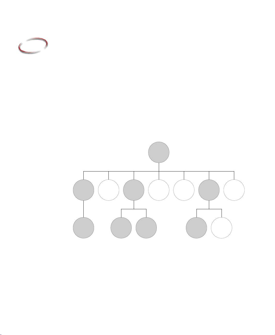
The bill of materials for BizBikes contains three levels, as shown below, for a generic end item. There are actually four end items (or BizBikes), 15 unique manufactured items, and five purchased parts. The shaded items in the bill of materials represent manufactured components. This generic bill of materials also includes information on manufacturing lead times, number required per subassembly, and lot size information.

FINAL

ASSEMBLY

AND PACK

(1,1,1)

FINISHED

FRAME (1,1,24)

FRAME (4,1,50)

KEY: (Lead Time, Quantity, Lot Size)

PEDAL AND

CHAIN

ASSEMBLY

(3,1,60)

HANDLEBAR

(3,1,100)

HANDLEBAR

ASSEMBLY

(1,1,75)

NECK POST

(3,1,60)

WHEELS

(3,1,48)

DERAILLEUR

ASSEMBLY

(4,1,60)

SEAT POST

(3,1,100)

SEAT

ASSEMBLY

(1,1,75)

SEAT

(2,1,100)

BRAKES

(2,1,75)

The Manufacturing Resource Planning system

BizBikes employs a Manufacturing Resource Planning (MRP) system that performs master planning and scheduling of weekly production. The MRP system consolidates orders from multiple customers and plans the purchase and manufacturing of the associated components. The MRP produces a set of manufacturing orders that are released to the factory floor. These manufacturing orders are for both component parts

FACTORYTALK SCHEDULER USER’S GUIDE

• • • • •

(frames, handlebars, etc.) as well as final assemblies. The components are produced tostock and are consumed during the subassembly and the final assembly and pack of a bicycle. The MRP also nets together purchased components across multiple customer orders. The MRP netting operation generates purchase requests for component parts (brakes, wheels, seats, etc.) based on economic order quantities and lead times. The MRP system also plans out and issues purchase requests for materials consumed in manufacturing component parts. The purchase requests for both component parts and raw materials are issued to suppliers who then ship these components to our factory. In the final assembly, we combine the manufactured and purchased components into a bicycle, which is then packed and shipped to the customer.

The following table shows production requirements for a typical ten-day period. These manufacturing orders have been downloaded from the MRP and include orders for SHP and SSD bicycles in both red and blue, along with MRP-generated orders for components required during assembly. The 70 manufacturing orders include 33 orders for finished BizBikes, 25 subassemblies, and 12 component parts.

3 • THE FACTORY OVERVIEW

• • • • •

Order # Product Name

SHP Red 1 SHP Red Bicycle 15 2/11/03 11 PM 2/12/03 11 PM SHP Red 2 SHP Red Bicycle 9 2/12/03 11 PM 2/13/03 11 PM SHP Red 3 SHP Red Bicycle 8 2/13/03 11 PM 2/14/03 11 PM SHP Red 4 SHP Red Bicycle 12 2/14/03 11 PM 2/17/03 11 PM SHP Red 5 SHP Red Bicycle 17 2/17/03 11 PM 2/18/03 11 PM SHP Red 6 SHP Red Bicycle 20 2/18/03 11 PM 2/19/03 11 PM SHP Red 7 SHP Red Bicycle 9 2/19/03 11 PM 2/20/03 11 PM SHP Red 8 SHP Red Bicycle 7 2/20/03 11 PM 2/21/03 11 PM SHP Blue 1 SHP Blue Bicycle 11 2/10/03 11 PM 2/11/03 11 PM SHP Blue 2 SHP Blue Bicycle 6 2/11/03 11 PM 2/12/03 11 PM SHP Blue 3 SHP Blue Bicycle 4 2/12/03 11 PM 2/13/03 11 PM SHP Blue 4 SHP Blue Bicycle 14 2/13/03 11 PM 2/14/03 11 PM SHP Blue 5 SHP Blue Bicycle 11 2/14/03 11 PM 2/17/03 11 PM SHP Blue 6 SHP Blue Bicycle 16 2/17/03 11 PM 2/18/03 11 PM SHP Blue 7 SHP Blue Bicycle 8 2/18/03 11 PM 2/19/03 11 PM SHP Blue 8 SHP Blue Bicycle 6 2/19/03 11 PM 2/20/03 11 PM SHP Blue 9 SHP Blue Bicycle 15 2/20/03 11 PM 2/21/03 11 PM SSD Red 1 SSD Red Bicycle 11 2/10/03 11 PM 2/11/03 11 PM SSD Red 2 SSD Red Bicycle 9 2/11/03 11 PM 2/12/03 11 PM SSD Red 3 SSD Red Bicycle 8 2/12/03 11 PM 2/13/03 11 PM SSD Red 4 SSD Red Bicycle 14 2/13/03 11 PM 2/14/03 11 PM SSD Red 5 SSD Red Bicycle 12 2/17/03 11 PM 2/18/03 11 PM SSD Red 6 SSD Red Bicycle 7 2/18/03 11 PM 2/19/03 11 PM SSD Red 7 SSD Red Bicycle 6 2/19/03 11 PM 2/20/03 11 PM SSD Red 8 SSD Red Bicycle 12 2/20/03 11 PM 2/21/03 11 PM SSD Blue 1 SSD Blue Bicycle 5 2/11/03 11 PM 2/12/03 11 PM SSD Blue 2 SSD Blue Bicycle 16 2/12/03 11 PM 2/13/03 11 PM SSD Blue 3 SSD Blue Bicycle 9 2/13/03 11 PM 2/14/03 11 PM SSD Blue 4 SSD Blue Bicycle 12 2/14/03 11 PM 2/17/03 11 PM SSD Blue 5 SSD Blue Bicycle 8 2/17/03 11 PM 2/18/03 11 PM SSD Blue 6 SSD Blue Bicycle 13 2/18/03 11 PM 2/19/03 11 PM SSD Blue 7 SSD Blue Bicycle 18 2/19/03 11 PM 2/20/03 11 PM SSD Blue 8 SSD Blue Bicycle 15 2/20/03 11 PM 2/21/03 11 PM SHP Red Finished Frame 1 SHP Red Finished Frame 24 2/10/03 11 PM 2/11/03 11 PM SHP Red Finished Frame 2 SHP Red Finished Frame 24 2/13/03 11 PM 2/14/03 11 PM SHP Red Finished Frame 3 SHP Red Finished Frame 24 2/14/03 11 PM 2/17/03 11 PM SHP Red Finished Frame 4 SHP Red Finished Frame 24 2/17/03 11 PM 2/18/03 11 PM SHP Blue Finished Frame 1 SHP Blue Finished Frame 24 2/10/03 11 PM 2/11/03 11 PM SHP Blue Finished Frame 2 SHP Blue Finished Frame 24 2/13/03 11 PM 2/14/03 11 PM SHP Blue Finished Frame 3 SHP Blue Finished Frame 24 2/17/03 11 PM 2/18/03 11 PM SHP Blue Finished Frame 4 SHP Blue Finished Frame 24 2/19/03 11 PM 2/20/03 11 PM SSD Red Finished Frame 1 SSD Red Finished Frame 24 2/10/03 11 PM 2/11/03 11 PM

Order

Quantity Release Date Due Date

FACTORYTALK SCHEDULER USER’S GUIDE

• • • • •

Order # Product Name

SSD Red Finished Frame 2 SSD Red Finished Frame 24 2/12/03 11 PM 2/13/03 11 PM SSD Red Finished Frame 3 SSD Red Finished Frame 24 2/18/03 11 PM 2/19/03 11 PM SSD Blue Finished Frame 1 SSD Red Finished Frame 24 2/11/03 11 PM 2/12/03 11 PM SSD Blue Finished Frame 2 SSD Blue Finished Frame 24 2/13/03 11 PM 2/14/03 11 PM SSD Blue Finished Frame 3 SSD Blue Finished Frame 24 2/17/03 11 PM 2/18/03 11 PM SSD Blue Finished Frame 4 SSD Blue Finished Frame 24 2/18/03 11 PM 2/18/03 11 PM Handlebar Assembly 1 Handlebar Assembly 75 2/10/03 11 PM 2/11/03 11 PM Handlebar Assembly 2 Handlebar Assembly 75 2/12/03 11 PM 2/13/03 11 PM Handlebar Assembly 3 Handlebar Assembly 75 2/14/03 11 PM 2/17/03 11 PM Handlebar Assembly 4 Handlebar Assembly 75 2/17/03 11 PM 2/18/03 11 PM Handlebar Assembly 5 Handlebar Assembly 75 2/19/03 11 PM 2/20/03 11 PM Seat Assembly 1 Seat Assembly 75 2/10/03 11 PM 2/11/03 11 PM Seat Assembly 2 Seat Assembly 75 2/12/03 11 PM 2/13/03 11 PM Seat Assembly 3 Seat Assembly 75 2/14/03 11 PM 2/17/03 11 PM Seat Assembly 4 Seat Assembly 75 2/17/03 11 PM 2/18/03 11 PM Seat Assembly 5 Seat Assembly 75 2/19/03 11 PM 2/20/03 11 PM Handlebar 1 Handlebar 100 2/11/03 11 PM 2/14/03 11 PM Handlebar 2 Handlebar 100 2/12/03 11 PM 2/17/03 11 PM Handlebar 3 Handlebar 100 2/14/03 11 PM 2/19/03 11 PM Neck Post 1 Neck Post 60 2/11/03 11 PM 2/14/03 11 PM Neck Post 2 Neck Post 120 2/12/03 11 PM 2/17/03 11 PM Neck Post 3 Neck Post 60 2/14/03 11 PM 2/19/03 11 PM SHP Frame 1 SHP Frame 50 2/10/03 11 PM 2/14/03 11 PM SHP Frame 2 SHP Frame 50 2/11/03 11 PM 2/17/03 11 PM SSD Frame 1 SSD Frame 50 2/11/03 11 PM 2/17/03 11 PM SSD Frame 2 SSD Frame 50 2/12/03 11 PM 2/18/03 11 PM Seat Post 1 Seat Post 100 2/12/03 11 PM 2/17/03 11 PM Seat Post 2 Seat Post 100 2/14/03 11 PM 2/19/03 11 PM

Order

Quantity Release Date Due Date

The BizBikes manufacturing resources

The BizBikes manufacturing plant contains seven work cells (Cut, Machine, Bend, Weld, Finish, two Subassembly areas, and two Assembly and Pack areas), and a three-person labor pool per shift (labor required by Subassembly and Assembly and Pack). All work cells and labor are available for two eight-hour shifts, five days a week (a 2/5 composite shift pattern). The first shift starts at 7 and ends at 11

PM. There are no scheduled breaks in either shift. The key differences for

the processes at the various work cells are summarized below. Keep in mind that all setup and process durations are expressed in hours.

AM and ends at 3 PM. The second shift starts at 3 PM

3 • THE FACTORY OVERVIEW

SSEMBLY AND PACK

These work cells are used to assemble and pack the finished BizBikes. The setup and process (per item) durations are part dependent. Each assembly operation requires two labor units from the labor pool for its entire duration.

UBASSEMBLY

These work cells are used to assemble component parts (manufactured and purchased) into subassemblies that are placed in stock for future required orders. The setup and process (per item) durations are part dependent. Each subassembly operation requires one labor unit from the labor pool for its entire duration.

INISH AND CUT

These work cells are utilized for operations necessary to produce the component parts required for the subassemblies. The setup and process (per item) durations are part dependent. These work cells are manned by a dedicated operation and do not require labor from the labor pool.

ACHINE AND BEND

These work cells are utilized for operations necessary to produce the component parts required for the subassemblies. The process (per item) durations are part dependent. These work cells are manned by a dedicated operation and do not require labor from the labor pool. The setup durations for these work cells are sequence dependent and defined in matrix MM for the Machine work cell and matrix BM for the Bend work cell. These two matrices are shown below.

• • • • •

Machine Setup Matrix: MM

SSD Frame SHP Frame Handlebar Neck Post

SSD Frame

SHP Frame

Handlebar

Neck Post

0.00 0.12 0.53 0.58

0.14 0.00 0.55 0.62

0.64 0.66 0.00 0.26

0.57 0.61 0.33 0.00

FACTORYTALK SCHEDULER USER’S GUIDE

• • • • •

This matrix shows the setup time for an operation based on the previous production lot that was processed at this work cell. For example, if the last production lot was Handlebar, then the setup time to produce a Neck Post is .26 hours.

Bend Setup Matrix: BM

SSD Frame SHP Frame Handlebar Neck Post

SSD Frame

SHP Frame

Handlebar

Neck Post

ELD

This work cell is also utilized for operations necessary to produce the component parts required for the subassemblies. The process (per item) durations are part dependent. These work cells are manned by a dedicated operation and do not require labor from the labor pool. The setup duration for this work cell depends upon the frame type; i.e., we have a different setup time for an SHP Frame and an SSD Frame. The setup time required to change to an SHP Frame is 0.72 hours, and the time required to change to an SSD Frame is 0.70 hours.

0.00 0.35 0.84 0.32

0.42 0.00 0.84 0.32

0.93 0.97 0.00 0.28

0.75 0.78 0.39 0.00

Process plans

There are eight different manufacturing order types, each with a different process plan or routing.

INAL ASSEMBLY AND PACK

The process plans for assembly and packing of the SHP Red, SHP Blue, SSD Red, and SSD Blue bicycles contain a single assembly operation. In this operation, a bicycle is assembled from its components and subassemblies and then packaged for shipping. The process plan for SHP Red Bicycle final assembly is summarized below.

SHP Red Bicycle Plan

Seq

10 Assemble

Operation Work Cell

and Pack

ASSEMBLE

AND PACK

Assembly and Pack

Setup

Process

Time

0.37 0.43 Labor (2) Components required

Time

Additional

Resources

Notes

3 • THE FACTORY OVERVIEW

The components required before this operation can be started are the manufactured parts SHP Red Finished Frame, Handlebar Assembly, and Seat Assembly and the purchased parts Pedal and Chain Assembly, Wheels, Derailleur Assembly, and Brakes.

INISHED FRAME

The process plans for a finished frame (SHP Red, SHP Blue, SSD Red, and SSD Blue) contain two operations. The frame parts are first finished (red or blue) and then the parts are subassembled. The finished frame is then placed in inventory where it is available for demand from a final assembly order. The process plan for SHP Red Finished Frame is summarized below.

SHP Red Finished Frame Plan

Seq

10 Finish SHP

20 Subassemble

Operation

Red Frame

SHP Frame

Work Cell

Finish 0.11 0.155 SHP Frame

Subassembly 0.19 0.083 Labor (1) Place in

Setup

Time

Process

Time

Additional

Resources

Notes

required

inventory

• • • • •

ASSEMBLE

FRAME

RAME

FINISH FRAME

The process plans for a frame (SHP or SSD) contain four operations: cut, bend, machine, and weld. The frame is then placed in inventory to be used by orders for finished frames. The raw materials required at both the cut and weld operations have not been included in the process plan as the material-planning replenishment process at the MRP level assures that adequate materials will be available. The process plan for

SHP Frame

is summarized next.

FACTORYTALK SCHEDULER USER’S GUIDE

• • • • •

SHP Frame Plan

Seq

10 Cut SHP Frame

20 Bend SHP Frame

30 Machine SHP

40 Weld SHP Frame Weld WD 0.234 Place in inventory

Operation

Tubing

Frame Tubing

Setup

Work

Cell

Time

Process

Time

Additional Resources

Notes

Cut 0.36 0.120

Bend BM 0.154

Machine MM 0.211

CUT FRAME

TUBING

ANDLEBAR ASSEMBLY

BEND FRAME

TUBING

MACHINE

FRAME

TUBING

WELD

FRAME

The process plans for the handlebar assembly contain a single subassembly operation. In this operation, the previously manufactured handlebars and neck posts are assembled. The subassembly is then placed in inventory where it is available for demand from a final assembly order. The component parts required for this subassembly are a handlebar and neck post for each subassembly to be produced. The process plan for Handlebar Assembly is summarized below.

Handlebar Assembly Plan

Seq

Operation Work Cell

10 Assemble

Handlebar

Subassembly 0.21 0.072 Labor (1) Handlebar and Neck

Setup

Time

Process

Time

Additional

Resources

Notes

Post required; Place in inventory

ASSEMBLE

HANDLEBAR

ANDLEBAR

The process plans for a handlebar contain three operations: cut, bend, and finish. The completed handle is then placed in inventory to be used by orders for handlebar assemblies. The raw materials required at the cut operation have not been included in the process plan as the material-planning replenishment process at the MRP level assures that

3 • THE FACTORY OVERVIEW

adequate materials will be available. The process plan for Handlebar is summarized below.

Handlebar Plan

Setup

Seq

# Operation Work Cell

10 Cut

Cut 0.16 0.055

Time

Process

Time

Additional

Resources

Notes

Handlebar Tubing

20 Bend

Bend BM 0.043 Handlebar Tubing

30 Finish

Finish 0.14 0.088 Place in inventory Handlebar

• • • • •

CUT

HANDLEBAR

TUBING

ECK POST

BEND

HANDLEBAR

TUBING

FINISH

HANDLEBAR

The process plans for a handlebar contain four operations: cut, machine, bend, and finish. The completed neck post is then placed in inventory to be used by orders for handlebar assemblies. The raw materials required at the cut operation have not been included in the process plan as the material-planning replenishment process at the MRP level assures that adequate materials will be available. The process plan for Neck Post is summarized below.

Neck Post Plan

Setup

Seq

# Operation Work Cell

10 Cut Neck

Cut 0.21 0.065

Time

Process

Time

Additional

Resources

Notes

Post

20 Machine

Machine MM 0.120

Neck Post

30 Bend Neck

Bend BM 0.072

Post

40 Finish Neck

Finish 0.14 0.074 Place in inventory

Post

CUT NECK

POST

MACHINE

NECK POST

BEND NECK

POST

FINISH NECK

POST

FACTORYTALK SCHEDULER USER’S GUIDE

• • • • •

EAT ASSEMBLY

The process plans for the seat assembly contain a single subassembly operation. In this operation, the previously manufactured seat post and purchased seat are assembled. The subassembly is then placed in inventory where it is available for demand from a final assembly order. The component parts required for this subassembly are a seat post and seat for each subassembly to be produced. The process plan for Seat Assembly is summarized below.

Seat Assembly Plan

Seq

# Operation Work Cell

10 Assemble

Seat and Post

ASSEMBLE

SEAT AND

POST

EAT POST

The process plans for a seat post contain two operations: cut and machine. The completed seat post is then placed in inventory to be used by orders for seat assemblies. The raw materials required at the cut operation have not been included in the process plan as the material-planning replenishment process at the MRP level assures that adequate materials will be available. The process plan for Seat Post is summarized below.

Setup

Time

Process

Time

Additional

Resources

Notes

Subassembly 0.20 0.084 Labor (1) Seat and Seat Post

required; Place in inventory

Seat Post Plan

Seq

# Operation Work Cell

10 Cut Seat

Cut 0.17 0.068

Post

20 Machine

Machine MM 0.130 Seat Post

Seat Post

CUT SEAT

POST

MACHINE

SEAT POST

Setup

Time

Process

Time

Additional

Resources

Material

Consumed

Material

Produced

3 • THE FACTORY OVERVIEW

Purchased components

In addition to the manufactured components, we also have purchased components that are used in the assembly operations. Purchase orders for these components are automatically generated by the MRP (based on the economic lot size and lead times) to meet the manufacturing demands. The following table summarizes the purchased components for this same sample ten-day production period.

Material Name Quantity Date

Pedal and Chain Assembly 60 6/10/02 6:00 PM Pedal and Chain Assembly 60 6/13/02 6:00 PM Pedal and Chain Assembly 60 6/19/02 6:00 PM Brakes 75 6/12/02 6:00 PM Brakes 75 6/18/02 6:00 PM Wheels 48 6/12/02 6:00 PM Wheels 48 6/17/02 6:00 PM Wheels 48 6/19/02 6:00 PM Derailleur Assembly 60 6/12/02 6:00 PM Derailleur Assembly 60 6/17/02 6:00 PM Derailleur Assembly 60 6/20/02 6:00 PM Seat 100 6/10/02 6:00 PM

• • • • •

FACTORYTALK SCHEDULER USER’S GUIDE

• • • • •

Inventories

We have a starting inventory level for both the manufactured and the purchased material. The following table summarizes the starting inventory of these items.

Material Type Initial Quantity

SHP Red Bicycle Make 0 SHP Blue Bicycle Make 0 SSD Red Bicycle Make 0 SSD Blue Bicycle Make 0 SHP Red Finished Frame Make 8 SHP Blue Finished Frame Make 16 SSD Red Finished Frame Make 17 SSD Blue Finished Frame Make 6 Handlebar Assembly Make 27 Seat Assembly Make 36 SHP Frame Make 97 SSD Frame Make 54 Seat Post Make 127 Handlebar Make 155 Neck Post Make 118 Pedal and Chain Assembly Buy 15 Brakes Buy 50 Wheels Buy 54 Derailleur Assembly Buy 54 Seat Buy 54

Previously scheduled orders

Finally, we have previously scheduled orders planned for completion. These orders are shown below.

Material Name Quantity Date

Seat Post 100 2/12/03 6:00 PM Neck Post 60 2/12/03 6:00 PM SSD Frame 50 2/12/03 6:00 PM

Summary

Now that we have described the BizBikes manufacturing process, we’ll use the information in the tutorial to illustrate the features of FactoryTalk Scheduler in Chapter 4.

Scheduling Features

FactoryTalk Scheduler provides a wide range of features for modeling constrained scheduling systems. There are four basic categories of modeling constraints available— resource, sequencing, material, fixture, and operation. We will discuss the major features for each of them and use the BizBikes tutorial from Chapter 3 to demonstrate examples.

Resource constraints

FactoryTalk Scheduler provides full support for the scheduling of constrained resources with four distinct resource types:

 Singular  Infinite  Simultaneous  Adjustable Pooled

The resource types differ in the functionality that they provide in modeling a wide variety of production environments.

The Singular resource is the most commonly used type. It represents a single machine, person, device, jig, fixture, or any resource that is constrained and has a capacity of one.

Tuto rial

Bend, Cut, Finish, Machine, Weld, Subassembly, and Assembly and Pack, as each resource can only perform one operation at a time.

The Infinite resource type provides the ability to represent resources that have an unlimited capacity. The most common example is a subcontractor or a drying area. Although a subcontractor has a theoretical infinite capacity, it still requires time to complete the task and may work only a single shift.

Tuto rial

The Simultaneous resource type represents resources that may have the ability to handle multiple activities. It is further restricted in that if a Simultaneous resource processes multiple activities at the same time, all the activities must be synchronized. This means that they must all start and end at the same time. The significance of this feature is best described by considering a kiln with a capacity measured in cubic feet. The kiln can be used to process any number of parts, as long as the volume of the parts does not exceed the kiln capacity. The synchronized restriction means that once you load and start the kiln, you must finish that process before it can be used to process any additional parts. You can

: For our tutorial system, we will model the resources as Singular in work cells

: We will not use this resource type in our tutorial system.

FACTORYTALK SCHEDULER USER’S GUIDE

• • • • •

also restrict what operations can be processed at the same time by requiring that certain operation attributes match before they can be processed together.

Tuto rial

The Adjustable Pooled resource type is most often used to represent pools of like resources, any one of which fulfills the requirement of the task or operation being performed. Typical examples are labor pools, totes, fixtures, or space. The number of units of an Adjustable Pooled resource can vary during the operation span. We will elaborate on this difference shortly.

Tuto rial

: We will not use this resource type in our tutorial system.

: The labor pool in our tutorial will be modeled as an Adjustable Pooled resource.

Primary and additional resources

Each operation to be scheduled must have a single primary resource for the entire duration of the operation. Operation durations can be separated into three phases. Normally, these are referred to as setup, process, and teardown. Additional resources can be specified for the entire operation or for an individual phase of the operation. There is no limit on the number of additional resources that an operation may require. However, as the number of additional resources increases, the scheduling problem becomes more complex. This will result in more time being required to develop a solution.

Shift patterns and efficiency

You can associate shift patterns, preventive maintenance, downtimes, etc., with any resource. In addition to shift patterns, you can also associate an efficiency, expressed as a fraction, with Singular, Infinite, and Simultaneous resources. Typically, this efficiency would be defaulted to 1.0. By changing the efficiency, you can speed up or slow down those operations that use the resource.

Resource sets

FactoryTalk Scheduler schedules to either a resource or a resource set. A resource set contains one or more resources. When a resource set contains multiple resources, the resources are typically of the same type, although it is not required. Likewise, it is not required that the names used for resource sets differ from those of resources, but this is the most common naming convention. Furthermore, a resource may be included in more than one set.

Tuto rial

Machiner, Welder, and Labor. You might note that although Labor is a single resource, it will have a capacity greater than one. We also have two resource sets, Subassembly Areas and Assembly and Pack Areas, each with two resources. The two subassembly resources are called Subassembly Area 1 and Subassembly Area 2. The two assembly resources are

: In our tutorial system, we will have six resources: Bender, Cutter, Finisher,

4 • SCHEDULING FEATURES

called Assembly and Pack Area 1 and Assembly and Pack Area 2. We will associate a 1/5shift pattern with all the resources.

The combination of the availability of required resources and resource efficiencies determine both where and how FactoryTalk Scheduler places an operation on the planning board during the scheduling process. A resource becomes unavailable for use by an operation in a given time period if it is currently being used by another operation or if it is in an off-shift state.

Simultaneous, Singular, and Infinite resource spanning

Consider an operation that requires two hours of processing time on a Singular resource. Assume that the resource is continuously on-shift starting at 7 shift the rest of the day. Also assume that there are no other operations currently using the resource. If the operation were unable to start until 12:30 would schedule the operation from 12:30

PM to 2:30 PM, taking a continuous two-hour

span of time. However, if the operation were unable to start until 2 Scheduler would schedule the operation to start at 2

PM on the current day, where it would

process for one hour. It would then resume processing the next day at 7 the two-hour operation by 8

AM.

AM until 3 PM and is off-

PM, FactoryTalk Scheduler

PM, FactoryTalk

AM to complete

• • • • •

When an operation crosses a time where a resource is in an off-shift state or at a reduced efficiency, it is called spanning. If an operation requires several secondary resources with different shift patterns, the spanning can become quite complicated. However, as long as all the required resources are Simultaneous, Singular, or Infinite types, no other operations can use these resources during the span time of the scheduled operation. Note that if one of these resources is a Simultaneous type, other operations may use any excess capacity.

Adjustable Pooled resource spanning

Adjustable Pooled resources differ not only in the manner in which resource spanning is allowed, but also because you can elect to not allow certain types of spanning for individual Adjustable Pooled resources. We’ll first discuss the default spanning mode.

The spanning behavior of Adjustable Pooled resources is best illustrated with an example.

The diagram below shows the availability profile of a labor resource. This profile represents a 2/5 shift pattern with three workers available during the first shift (7

PM), two available during the second shift (3 PM to 11 PM), and none available during the

3 third shift. Note that the diagram shows that there is currently an operation, represented by the white area, which has been allocated one labor unit from 10

AM to 9 PM on Day 1.

AM to

FACTORYTALK SCHEDULER USER’S GUIDE

• • • • •

7 101 4 7101 4 710

AM PM AM

Let us assume that FactoryTalk Scheduler is going to schedule an operation that requires a primary resource that is available 24 hours a day and currently is not being used during Days 1 or 2. This operation also requires two units of labor during its six-hour operation time. If the operation were available to start on or before 9 scheduled during the first day. For example, if the operation could start at 8 be scheduled from 8

AM of Day 1, it could be

AM, it would

AM to 2 PM, as shown below.

7 101 4 7101 4 710

AM PM AM

Adjustable Pooled resources not only allow spanning, but they also allow the number of labor units to vary, which will pace the operation. Thus, Adjustable Pooled resources are often used to model resources where the pace or efficiency of the operation is based on the number of workers currently available. Again, this is best illustrated using an example.

Let’s assume that we want to schedule the same six-hour operation as before. If the operation could not start until 1

PM on Day 1, it would be scheduled from 1 PM to 10 PM,

4 • SCHEDULING FEATURES

as shown below. Although this operation time is six hours, this particular process spans a nine-hour period because it’s paced by the labor availability.

7 101 4 7101 4 710

AM PM AM

• • • • •

Between 1 is assumed to be at 100% efficiency during that time. However, between 3

PM and 3 PM, there are two units of the resource available. Thus, the operation

PM and 9 PM,

there is only one unit of labor available. The operation will continue during this six-hour period at 50% efficiency, which accounts for an additional three hours of operation time. During the last hour of the operation, the efficiency returns to 100% because two labor units are available.

The spanned operation time can also include periods when there are no units available, resulting in a zero efficiency during that time. The total number of units requested must be available when the operation starts. For example, if the operation could not begin until

PM of Day 1, the start of the operation would have to be delayed until 9 PM on Day 1 and

4 would finish at 11

7 101 4 7101 4 710

AM PM AM

AM on Day 2, as shown below.

FACTORYTALK SCHEDULER USER’S GUIDE

• • • • •

Although the operation could start at 4 PM, there is only one unit of labor available from

PM to 9 PM, so the scheduled start of the operation would be at 9 PM when there are two

3 units available. From 9 the first two hours of the operation. From 11 units available, resulting in zero efficiency. The last four hours of the operation occur at 100% efficiency with two units available from 7

You also have the option of specifying a minimum number of units that must be available for the operation to continue (the default is zero). This minimum value must be fewer than or equal to the total number of units requested. Let’s consider the same six-hour operation with a minimum equal to the total number, or two units. If the operation cannot start until

PM on Day 1, it would be scheduled from 1 PM to 9 AM of Day 2, as shown below. This

1 particular process spans a 12-hour period because it requires two units during the entire operation. Thus, it spans the time from 3

PM to 11 PM, the operation is at 100% efficiency—accounting for

PM of Day 1 to 7 AM of Day 2, there are no

AM to 11 AM of Day 2.

PM to 9 PM where there is only one unit available.

7 101 4 7101 4 710

AM PM AM

Consider an example where the total number of units required is five and the minimum number of units is three. The operation could not start until there were five units available, and it would continue as long as there were three or more units available, although it would occur at a lower efficiency if there were only three or four units available during that time. If the operation is started and there is a point where there are fewer than three units available, the operation will span (at zero efficiency) this time until there are at least three units available, at which time it would resume.

As mentioned earlier, you can also elect to not allow certain types of spanning for specific Adjustable Pooled resources. If you make this election, it will allow spanning to occur during off-shift states, but it will not allow spanning where the resource is unavailable because it is being used by another operation.

Sequencing constraints

Sequencing constraints are normally a part of the product or job routing and determine the sequence in which operations can be performed. Many systems have simple or straight routings where the sequence is simply determined by the order in which the operations are listed. The first operation must be completed before the second one can start, the second completed before the third can start, and so on. Other systems allow parallel or concurrent operations in their routings. These types of systems often include assembly or disassembly operations. The most difficult sequencing constraints are found in systems where routings are represented as networks. These types of routings are most frequently found in maintenance operations.

FactoryTalk Scheduler provides complete support for all types and combinations of sequencing constraints. There are two different ways to describe sequencing constraints: using an operation sequence numbering scheme or using an immediate successor operation(s) scheme. The two methods cannot be used together in the same application. All sequencing constraints for a given application must be described using the same scheme.

The operation sequence numbering scheme

The operation sequence numbering scheme has the following format:

• • • • •

4 • SCHEDULING FEATURES

XX.YY.YY.YY…

where:

XX is the standard integer operation sequence number and will be referred to as the root operation number

YY is the integer suffix that can be appended to the basic number, separated by the decimal character “.”

You can append as many suffixes as needed to represent your routings accurately. The rules used by FactoryTalk Scheduler to determine the sequence of operations are:

1. If the operation sequence number consists of only a root operation number (only XX), then all operations with lower root numbers (ignoring all suffixes) must precede that operation. Conversely, all operations with higher root numbers (ignoring all suffixes) must succeed that operation. Note that it is possible to have one or more operations with the same root number, with or without suffixes.

2. If the operation sequence number consists of a root operation number and one or more suffixes, then:

 all operations with lower root numbers and the same exact suffixes must precede

that operation,

FACTORYTALK SCHEDULER USER’S GUIDE

• • • • •

 all operations with lower root numbers and a fewer number of suffixes must

precede that operation, as long as the remaining suffixes match,

 all operations with lower root numbers and the same suffixes, but with additional

appended suffixes must precede that operation, and

 the converse defines the operations that succeed that operation.

The immediate successor operation(s) scheme

The operation number in the immediate successor operation scheme does not include any sequence information. The sequence of operations is determined by specifying an additional operation field, called the immediate successor operation attribute. The rules for this scheme are:

 each operation in a routing must have a unique job step number,  the operation numbers cannot include suffixes,  the immediate successor operation attribute field defines the immediate successor

operation job step number,

 if an operation has no successor, the immediate successor operation attribute field is

left blank, and

 if an operation has multiple successors, the job step numbers are separated by the “&”

character.

Sequencing constraint examples

A set of examples will best explain these rules and illustrate the differences between the two schemes. In the following examples, we include both a routing diagram to illustrate the operation sequence numbering scheme and a successor table to illustrate the immediate successor operation scheme. In most of the examples, the operation numbers will be different. In those examples, both operation numbers will be displayed in the routing diagrams, with the immediate successor operation numbers in parentheses “( )”. Both operation numbers will also be included in the successor table. The operation sequence numbering scheme operation numbers will be labeled as OSN scheme operation number, and the immediate successor operation scheme operation numbers will be labeled as ISO scheme operation numbers.

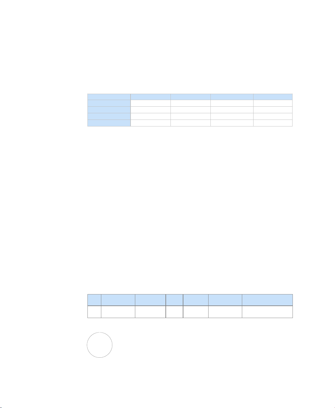
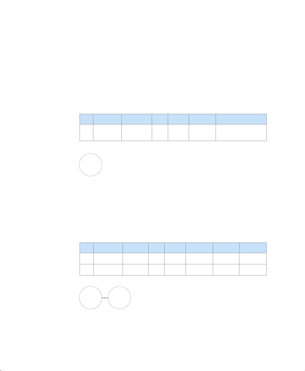
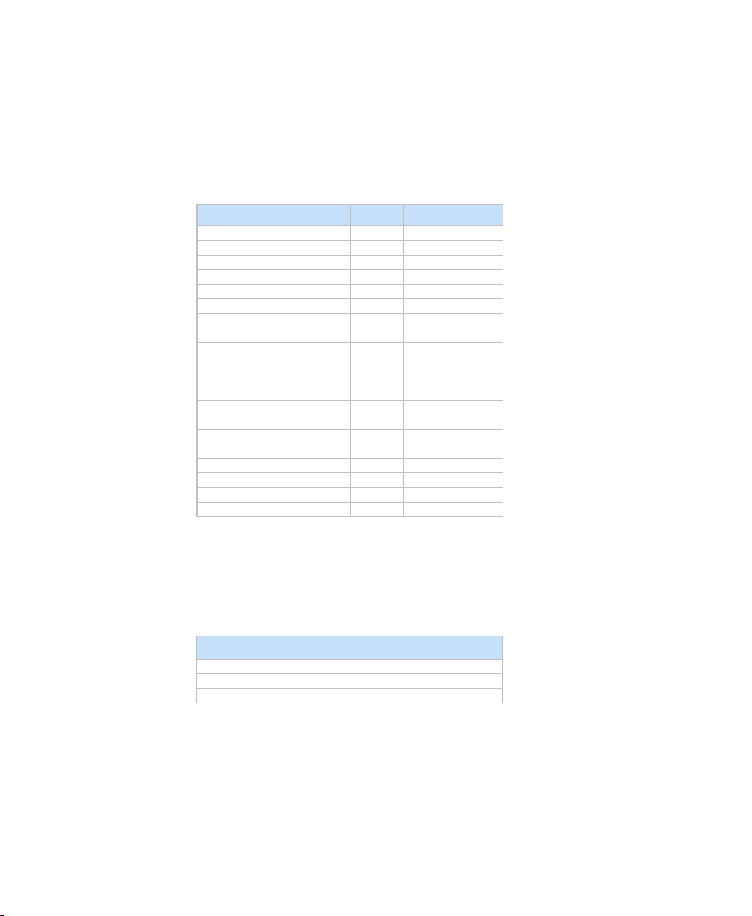
If you have simple straight-line routings with no assembly or disassembly, then you only need to use root operation numbers. You can also describe one operation assembly or disassembly routing using only root operation numbers. Our first example shows two parallel operations, labeled 10, which can be performed independently, but both need to be completed before the last operation, labeled 20, can be started.

4 • SCHEDULING FEATURES

(10)

(30)

(20)

Immediate Successor Table

OSN Scheme Operation

Number

10 10 30

10 20 30

20 30

ISO Scheme Operation

Number

Immediate Successor

Operation Number

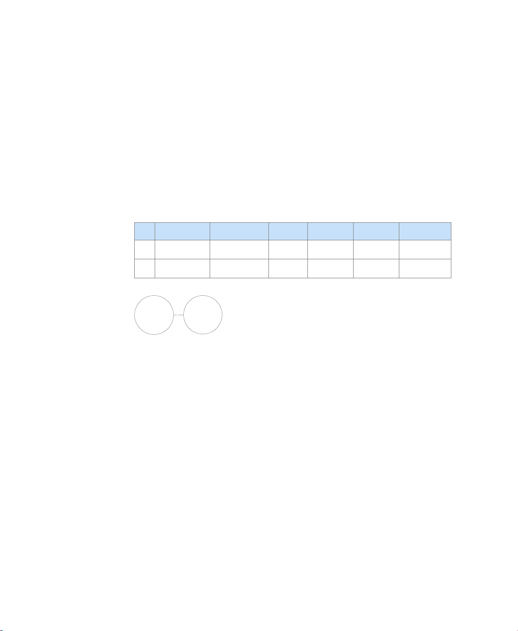
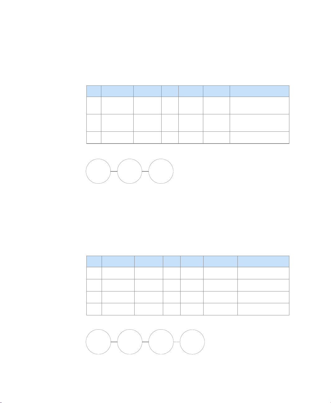
The second example extends the previous one by allowing two sets of parallel operations. In this example, the first two operations, labeled 10, can be performed independently, but both need to be completed before the next two operations, labeled 20, which can be performed independently.

• • • • •

(20)

OSN Scheme Operation

Number

10 10 30 & 40

10 20 30 & 40

20 30 50

20 40 50

30 50

(30)

(50)

(40)

Immediate Successor Table

ISO Scheme Operation

Number

Immediate Successor

Operation Number

FACTORYTALK SCHEDULER USER’S GUIDE

• • • • •

The third example illustrates how to use the numbering schemes to allow a series of operations to be performed independently, as would normally be the case in typical industrial routings. This example has both assembly and disassembly features. In this example, the first two operations with the “1” suffix can be performed independent of the first two operations with the “2” suffix. You can use any value for a suffix, as shown in the disassembly portion of the example, where we skip to a “5” suffix.

10.1 (10)

10.2 (30)

OSN Scheme Operation

Number

10.1 10 20

20.1 20 50

10.2 30 40

20.2 40 50

40.1 60 100

40.2 70 100

40.5 80 90

45.5 90 100

40.1

20.1 (20)

20.2 (40)

30 50 60 & 70 & 80

50 100

(50)

Immediate Successor Table

ISO Scheme Operation

Number

(60)

40.2 (70)

40.5 (80)

(100)

45.5 (90)

Immediate Successor

Operation Number

The fourth example shows a complicated bill of materials that requires several assembly operations at different levels. This numbering scheme illustrates the flexibility of representing complex routing structures.

4 • SCHEDULING FEATURES

• • • • •

10.1.1.1 (10)

10.1.1.2 (30)

10.1.2 (50)

10.1.3 (70)

20.1.1.1 (20)

20.1.2 (60)

OSN Scheme Operation

Number

10.1.1.1 10 20

20.1.1.1 20 40

10.1.1.2 30 40

30.1.1 40 110

10.1.2 50 60

20.1.2 60 110

10.1.3 70 80 & 90

20.1.3.1 80 100

20.1.3.2 90 100

30.1.3 100 110

40.1 110 130

40.2 120 130

50 130

20.1.3.1 (80)

20.1.3.2 (90)

30.1.1 (40)

30.1.3

(100)

Immediate Successor Table

ISO Scheme Operation

Number

40.1

(110)

40.2

(120)

Immediate Successor

Operation Number

(130)

FACTORYTALK SCHEDULER USER’S GUIDE

• • • • •

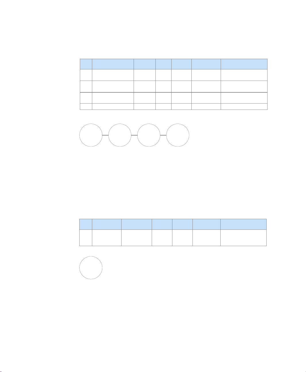
The final example illustrates a non-traditional network routing structure. Project management and maintenance environments frequently use these types of networks. This example illustrates the flexibility of the two numbering schemes.

20.1.2 (20)

(10)

20.1 (30)

OSN Scheme Operation

Number

10 10 20 & 30

20.1.2 20 40

20.1 30 40 & 50

30.1.2 40 60

30.1.1 50 60

40 60

30.1.2 (40)

30.1.1 (50)

Immediate Successor Table

ISO Scheme Operation

Number

(60)

Immediate Successor

Operation Number

Most industrial applications use the operation sequence numbering scheme because their routings tend to follow a straight line with occasional assembly operations. In addition, this scheme directly supports the routing numbering scheme used by most Enterprise Resource Planning (ERP) and Manufacturing Resource Planning (MRP) systems. The immediate successor operation scheme is generally only used when routings are more like a network as shown in our last example.

Tuto rial

: The routings for our tutorial system are simple routings in that only root numbers are required to describe the sequencing constraints. Thus, we have chosen to use the operation sequence numbering scheme. Recall that routing diagrams using this scheme were included in the previous chapter.

Material constraints

Material constraints typically are used to represent any make-to-stock or purchased items that constrain the scheduling of operations. This information is normally found in the

4 • SCHEDULING FEATURES

product bill of materials and indicates the amount of each material item required and where in the routing it is required. FactoryTalk Scheduler combines the bill of materials detail with the routing information.

You might think of a material as a bucket or bin containing inventory items of the same type. In FactoryTalk Scheduler, you can replenish or add to a material at the completion of any operation in a product routing, although in a make-to-stock environment, you would typically add to the material after the completion of the last operation of the product routing. You can also add to material based on the receipt of a purchase request for that item. It is not necessary to define an item as only a make-to-stock or purchased item; either method can replenish any material item. Material can also be consumed or removed at any operation in a product routing. When a material(s) is required by an operation, that operation will normally not be scheduled until all of the required material is available.

You can elect that material be consumed and/or produced in batches. For example, your production order batch size for a given material may be 1,000, but the actual material is transferred in batches of 100. By activating the batch transfer option for selective material actions, you can allow material to be available for consumption by other operations before the operation producing the item has been completed.

The replenishment or consumption of material is referred to as a material action. You can have as many material actions of either type as are required at any operation. For each material action, you must determine whether the replenishment or consumption is based on a quantity, which defaults to one, or the operation batch size. This determination is made at the operation level; thus, you can base the action on a quantity at one operation and the operation batch size at another operation. Note that if an operation batch

quantity has not been specified, this quantity defaults to the order quantity.

• • • • •

In a typical ERP or MRP environment, all lower-level items have product routings that result in items being added to a material, based on the operation batch quantity. Higherlevel items that require these materials are not scheduled until the materials become available. Thus, the MRP system takes care of the product explosion, netting of lowerlevel items, and the lead-time offset in scheduling the replenishment of materials. FactoryTalk Scheduler then makes sure that the required lower-level materials or items are available in developing a schedule.

When FactoryTalk Scheduler attempts to schedule an operation that requires a material, it will only schedule that operation at or after the time that the material level is sufficient to meet the requirements. If the scheduling horizon does not meet that condition, FactoryTalk Scheduler will first look to see if there are any unallocated orders that would produce the required material. If it finds such an order(s), it will first schedule that order(s), then schedule the operation requiring the material. If the order that produces the material requires another unavailable material, FactoryTalk Scheduler will look for an order to schedule as before. This process will be repeated as many times as required in an

FACTORYTALK SCHEDULER USER’S GUIDE

• • • • •

attempt to allow the scheduling of the initial item. If there are insufficient materialreplenish orders to allow the final item to be scheduled, FactoryTalk Scheduler will not schedule the final item and will remove all items scheduled in the attempt to produce the material requirements.

Tutorial

replenished as purchased items and consumed by the production of other products: Pedal and Chain Assembly, Wheels, Derailleur Assembly, Seat, and Brakes. The materials Frame, Handlebar, Neck Post, and Seat Post will be replenished by production orders and consumed by subassembly orders. The materials Finished Frame, Handlebar Assembly, and Seat Assembly will be replenished by production orders and will consume other materials. The Final Assembly and Pack order will consume many of the previously mentioned subassembly and purchased materials.

: In our tutorial, the following items will be modeled as materials, which are

Fixture constraints

Fixture constraints can be used to model fixtures, tooling, molds, or special materialhandling devices that can be required for more than one successive operation. For ease of definition, we’ll classify all of these types of devices as “fixtures.” Fixtures differ from materials in that they are not consumed or produced, although you can vary the number of available fixtures over time.

A fixture(s) can be required at any operation and held across several following operations in the same process plan. One operation seizes a number of fixture units and a following operation releases the units. It’s important to note that the fixture must be released in the same process plan in which it is seized. It is also possible to seize a fixture at the start of an operation and release it at the end of the same operation.

Tutorial

: This concept is not illustrated in our tutorial.

Operation constraints

In addition to resource, sequencing, and material constraints, there are a number of operation constraints that can be included in a FactoryTalk Scheduler configuration. We won’t attempt to cover all these special features in this chapter; we’ll only highlight a few of the most commonly used features.

FactoryTalk Scheduler provides several features that can alter the way resource setups constrain the schedule. Most frequently used is the sequence-dependent setup feature that allows the setup time used for the current operation to be dependent on both the current and last operation. FactoryTalk Scheduler provides the ability to reference a setup matrix that includes these times when it is scheduling the operation.

Tuto rial

and Bend work cells.

: We use this feature in our tutorial to represent the setup times at the Machine

A similar feature allows an operation process time to have a resource product

dependency.

FactoryTalk Scheduler also provides several features that determine how setups and/or teardowns are scheduled. These allow for multiple times, which can be performed in

parallel or sequential fashion. They also allow these activities to be performed in off-shift time periods.

Additional features provide more control on the timing between successive operations. These allow for the overlapping of operations at one extreme to the delay of the start of a subsequent operation at the other extreme.

You can also place limits on the total span of an operation to prevent a specific operation from spanning off-shift times, such as weekends.

These are just a sampling of the more commonly used special features that can be included in a FactoryTalk Scheduler configuration.

Summary

Now that we have reviewed the basic modeling features of FactoryTalk Scheduler using resource, sequencing, material, and operation constraints, let’s turn our attention to a discussion of finite-capacity scheduling procedures.

• • • • •

4 • SCHEDULING FEATURES

FACTORYTALK SCHEDULER USER’S GUIDE

• • • • •

Scheduling Concepts

FactoryTalk Scheduler incorporates both an algorithmic and a simulation-based scheduler. This chapter describes finite-capacity scheduling in general, details the differences between these scheduling methods, and discusses how to select scheduling rules to accomplish your objectives.

Finite-capacity scheduling

Finite-capacity scheduling (FCS) is the process of creating a production schedule for a set of jobs that is to be produced using a limited set of resources. Each job is comprised of one or more operations (machine, form, paint, etc.) that must be performed in a specified sequence using the set of available resources (work-centers, machines, workers, etc.). A schedule assigns a starting and ending time to each operation and sequences the operations across the resources so that no resource conflicts occur. The operations are also assigned in a way that any sequencing constraints are respected.

FCS can be done using a manual planning board (sometimes called a Gantt chart) in which the available resources are listed down the left side. The operations are assigned to the resource rows and spaced horizontally within each row to represent the passage of time. Each operation is represented by a horizontal bar where the length of the bar represents the duration of the operation.

CHEDULING EXAMPLE

The figure below shows a simple planning board with one of many possible operation schedules for three different jobs, denoted as Jobs A, B, and C. These jobs are produced using two resources denoted as Resources 1 and 2. The label within each horizontal bar denotes the job sequence (e.g., A-10 denotes Job A, Sequence Number 10). The data defining the operations for each job are shown in the accompanying table.

Resource 1

Resource 2

B-20A-10 C-10

B-10 A-20 C-20

Time

51015

FACTORYTALK SCHEDULER USER’S GUIDE

• • • • •

Job Sequence Resource Processing Time

A101 3

A202 4

B102 5

B201 2

C101 3

C202 4

In this simple example, Job A consists of two operations that are defined by sequence numbers 10 and 20 and must be performed in that order. Operation 20 cannot begin until Operation 10 is complete. Jobs B and C also contain two operations numbered 10 and 20, respectively. The processing time for each operation is also shown in the table.

It is important to note that this is merely one of several possible production schedules that can be generated for this very simple two-resource, three-job problem. In practical problems involving many different resources and many different jobs, the number of possible schedules is enormous. We clearly need an effective method for generating a good schedule that meets our production objectives.

Let’s now turn our attention to the general FCS problem.

 Given: A set of jobs and a limited set of resources  Find: A “good” schedule

Note that the objective is defined as determining a “good” schedule rather than an “optimal” schedule. We state our problem like this for two reasons. First, large scheduling problems (i.e., those with many resources and many jobs) are typically computationally challenging, and it’s not possible to achieve an “optimal” solution in a reasonable time. Second, there are typically several simultaneous objectives (minimize tardiness, minimize cycle time, maximize resource utilization, etc.), and these are often in conflict. In a practical setting, therefore, we strive to find a “good” solution that balances these objectives and can be obtained with minimal computation.

We will describe two fundamentally different approaches to constructing a schedule. The first is algorithmic, or job-at-a-time sequencing. The second is simulation-based, or operation-at-a-time sequencing.

Algorithmic sequencing

Algorithmic sequencing is a simple method for schedule construction. The algorithmic sequencer selects a job and then puts each operation for that job on the planning board. It

5 • SCHEDULING CONCEPTS

repeats this process until all jobs (and therefore, all operations) have been loaded. Each operation is loaded on its specified resource at the first available time slot that satisfies the constraints for that operation.

In a job-at-a-time sequencer, the schedule is controlled by selecting the order in which the jobs are loaded onto the planning board. Hence, the key to the quality of the schedule that is generated by the algorithmic sequencer is the rule that is used for selecting the jobloading order.

CHEDULING EXAMPLE

The job-at-a-time scheduling process is shown in the figures below. In this example, we first load Job A, then Job B, and finally, Job C.

• • • • •

Resource 1

Resource 2

Resource 1

Resource 2

Resource 1 A-10 C-10

Resource 2

A-10

A-20

51015

B-20

A-20

51015

A-20 C-20

51015

B-10

B-20

B-10

Time

Forward sequencing

There are a number of very simple heuristic rules that can be used to select the order for loading the jobs on the planning board. One rule that can be used for selecting the job order is to sort the jobs by a priority value that has been assigned to each job. Other possible sorting criteria are earliest due date, earliest release date, and smallest remaining slack time. None of these rules are optimal in a mathematical sense. Each rule represents a different strategy and focus in planning the jobs. For example, the due-date-related rules

FACTORYTALK SCHEDULER USER’S GUIDE

• • • • •

(due date and slack time) focus on reducing the number of late jobs, whereas the prioritybased rule strives to complete the most important jobs as soon as possible.

In some applications, a given operation can be performed on two or more different resources. For example, a drilling operation might be performed on either of two drills. In such cases, the schedule in an algorithmic sequencer is first determined by the ordering of jobs, then by the rule that is used to determine to which resource a given operation is assigned during the loading process. Again, simple heuristic rules (e.g., assign the operation to the resource that will complete the operation first) can be used to determine the schedule.

Backward sequencing

Although a job-at-a-time sequencer typically loads each job working forward in time by starting with the first operation and continuing through the last operation, it is also possible to use this same sequencing scheme but reverse the procedure to work backward in time. In this case, the sequencer begins by loading the job’s last operation to finish at its due date. It then continues by loading the job’s preceding operation to finish at the start time of the last operation. This process is continued, working backward in time, until the first operation for the job is loaded. At this point, the sequencer then selects a new job to load and repeats the entire process, again starting with the last operation and working backward in time. It continues in this fashion until all jobs are loaded.

CHEDULING EXAMPLE

The figure below shows a schedule generated by backward sequencing Jobs A, B, and C, where the vertical line on the right denotes the due date for all three jobs.

Resource 1

Resource 2

C-10 B-20A-10

B-10 A-20C-20

Time

51015

The advantage of a backward algorithmic sequencer is that it always generates a schedule that has no late jobs. However, the schedule may require start times that are infeasible; that is, the jobs must start before the current time. In essence, a forward job-at-a-time sequencer fixes the start times for a job and determines the end times (which may violate the due dates), whereas a backward job-at-a-time sequencer fixes the end times and determines the start times.

5 • SCHEDULING CONCEPTS

Although the idea of constructing a schedule that has no late jobs is appealing, backward sequencing has some practical limitations, even in cases where a feasible solution is generated. Backward scheduling shifts all jobs to the right on the planning board so that they start as late as possible while still meeting the due date. This means that there is no time buffer in the system, so any disruptions that occur (machine breakdowns, late material arrivals, etc.) will typically create late jobs. In addition, by postponing the use of our available capacity and waiting until the last minute to start each job, we give up the opportunity to consider additional jobs that may arrive later and need to be added to the schedule. For these reasons, many schedulers prefer a forward sequencer.

Bi-directional or bottleneck sequencing

It is also possible to use an algorithmic sequencer in a bi-directional or bottleneck mode. In this case, we select an operation somewhere in the middle of the job sequence and schedule the remaining operations using forward sequencing of the succeeding operations and using backward sequencing for the preceding operations. This is useful in cases where we have a bottleneck or highly utilized resource and we want to assign operations to this bottleneck resource and then load the upstream and downstream operations around it. The advantage of a bottleneck algorithmic sequencer is that it tends to minimize the cycle times of all jobs.

• • • • •

In summary, an algorithmic sequencer is a simple and fast method for loading a set of jobs on the planning board. The schedule is completely determined by specifying the order of jobs and a rule for selecting among resources.

Algorithmic job selection rules

Algorithmic job selection rules are used to determine the order in which the jobs are loaded onto the planning board. Most of them are simple ranking rules based on some attribute of the job. Brief descriptions of the standard algorithmic job selection rules are given below.

 Bottleneck: Ranking based on a secondary job selection rule. The forward and

backward mode schedules all unallocated jobs with emphasis on those operations that require a bottleneck resource. The bi-directional mode only schedules jobs that require an identified bottleneck resource. The user can then schedule the remaining jobs using any of the available job selection rules.

 Due Date: Ranking based on the earliest job due date first.

 First-Come, First-Served: Ranking based on the position in which they are entered

into the database.

 Ascending Order Property: Ranking based on the ascending value of a specified

order property. The order property can be numeric or character, and it must be specific

FACTORYTALK SCHEDULER USER’S GUIDE

• • • • •

as an available ranking order property. FactoryTalk Scheduler will automatically list all specified order properties.

 Priority: Ranking based on the smallest numeric priority. If you use this rule, a

priority field must be included in the order database.

 Process Time: Ranking based on the sum of the job’s operation times, the smallest

sum being ranked first.

 Release Date: Ranking based on the earliest job release (or early start) date first.

 Reverse Priority: Ranking based on the largest numeric priority. If you use this rule, a

priority field must be included in the order database.

 Slack Time: Ranking based on the smallest total job slack time.

 User Rule: Ranking based on a custom-written user rule. Multiple user rules can be

added with the name of each display on a secondary selection list.

Simulation-based sequencing

Simulation-based sequencing provides an attractive alternative to algorithmic sequencing by providing a simple, yet very flexible method for constructing a schedule. In general, any schedule that is produced by an algorithmic sequencer can also be produced by a simulation-based sequencer. A simulation-based sequencer, however, can also consider many schedules that cannot be considered by an algorithmic sequencer.

In contrast to the algorithmic sequencer, the simulation-based sequencer selects and loads an operation-at-a-time. By loading individual operations rather than entire jobs, the simulation-based sequencer has finer control over the way the operations are loaded onto the planning board. This operation-at-a-time loading is the key to the added flexibility in schedule generation using the simulation-based sequencer.

A second fundamental difference between the algorithmic and simulation-based sequencer is that the simulation-based sequencer constructs the schedule in a single time pass by moving forward from one event time to the next. The simulation-based sequencer begins at the current time and loads all operations that can start now. Note that these operations do not come from a single job as in the case of the job-at-a-time sequencer, but can be taken from the entire set of jobs. Once all operations are loaded that can start at this event time, the simulation-based sequencer advances time to the next event—e.g., the first completion time for any operation on the planning board. In this case, a busy resource has just changed to idle; hence, the simulation-based sequencer attempts to load additional operations at this new event time. The simulation-based sequencer continues in this fashion, advancing time forward to the next event time and loading additional operations as resources become idle, until all operations have been loaded.

5 • SCHEDULING CONCEPTS

CHEDULING EXAMPLE

The following sets of figures illustrate the simulation-based construction process. In each of the figures, the vertical line denotes the current value of simulated time.

TEP

1: L

OAD OPERATION

A-10

AND

B-10

• • • • •

Resource 1

Resource 2

TEP

2: L

Resource 1

Resource 2

TEP

3: L

Resource 1

Resource 2

A-10

B-10

51015

OAD OPERATION

A-10 C10

B-10

51015

OAD OPERATION

A-10 C10

B-10

51015

Time

C-10

Time

A-20

Time

FACTORYTALK SCHEDULER USER’S GUIDE

• • • • •

TEP

4: L

OAD OPERATION

B-20

Resource 1

Resource 2

TEP

5: L

Resource 1

Resource 2

A-10 C10

B-10

OAD OPERATION

A-10 C10

B-10

B-20

A-20

Time

51015

C-20

B-20

A-20

51015

C-20

Time

The first step in the simulation-based sequencer is to load all operations that can begin at the current time. In this example, Operation 10 for Job A (A-10) can be loaded on Resource 1, and Operation 10 for Job B (B-10) can be loaded on Resource 2. Next, the simulated time is advanced to the ending time of Operation A-10, and Operation C-10 is then loaded on Resource 1. Next, simulated time is advanced to the end of Operation B-10, and Operation A-20 is loaded on Resource 2. Next, simulated time is advanced to the end of Operation C-10, and Operation B-20 is loaded on Resource 1. Next, simulated time is advanced to the end of Operation B-20. Since no further operations remain to be loaded on Resource 1, simulated time is advanced to the end of Operation A-20 where the final operation, C-20, is loaded on Resource 2.

In contrast to the algorithmic sequencer, the simulation-based sequencer only moves time forward. It only advances time forward once all operations that are to be loaded at that time have been loaded. Hence, the simulation-based sequencer temporarily stops time and examines the entire job set, advancing to the next event time once all operations have been loaded. The algorithmic sequencer, on the other hand, is constantly moving back and forth in time as it loads all operations for each job. It starts at the current time and goes forward in time loading all operations for this first job. It then returns to the current time and again moves forward in time to load all operations for the second job. It continues in this fashion, moving forward and backward in time, until all jobs are fully loaded on the planning board. Hence, the algorithmic sequencer fixes a job and works across time, advancing to the next job once all operations have been loaded.

5 • SCHEDULING CONCEPTS

Selection rules

In a simulation-based sequencer, there are two types of selection rules that can be applied each time an operation is scheduled: an operation selection rule or a resource selection rule. If a resource becomes available and there are several available operations that require that resource, the operation selection rule is used to determine which operation is scheduled. If an operation becomes available and it can be scheduled on more than one resource, the resource selection rule is used to determine that resource. If both multiple operations and multiple resources are available, the operation rule is applied to select an operation, and then the resource rule is applied to select the resource.

Simulation-based sequencing can be set up so there is a single operation selection rule used to select all operations and a single resource selection rule to select all resources, or separate rules can be applied. If separate rules are used, they are associated with specific resource groups. For example, you may want to use a minimize setup rule for one group of resources and a due date rule for another.

Types of rules

There are two types of rules: independent and dependent. The use of independent rules allows different rules to be applied to the selection of operations and the selection of resources. Dependent rules require that the same rule be applied to the selection of both the operation and the resource. You can also develop and include your own rules. These are referred to as user rules, which will be included automatically on the list of available rules.

• • • • •

Although the operation-at-a-time loading scheme used by a simulation-based sequencer provides great flexibility in schedule generation, the key to tapping this flexibility is the development of rules for selecting the next operation to load or the resource on which it will be loaded. We discuss this in the following section.

Sequencing rules: The key to good schedules

The key to tapping the power and flexibility of simulation-based scheduling is the development of rules for guiding this two-step process. There are two basic categories of rules: operation selection rules (OSR’s) and resource selection rules (RSR’s). This section describes the basic concepts for incorporating rules into the FactoryTalk Scheduler simulation-based sequencer. One of the key advantages of a simulation-based sequencer is the ability to incorporate decision logic in the scheduling process based on rules for selecting operations and resources.

Operation selection rules

Operation selection rules, OSR’s, are invoked in FactoryTalk Scheduler whenever at least one resource is idle and two or more operations can be loaded on that resource. The rule

FACTORYTALK SCHEDULER USER’S GUIDE

• • • • •

determines which operation to load. This rule is the key factor that determines the quality of the resulting schedule.

ESOURCE GROUPS AND QUEUES

Before discussing the rule mechanisms in FactoryTalk Scheduler, we must first discuss the concept of Resource Groups and Queues. Each of the resources in the system may be assigned to one or more resource groups. These resource groups are used to represent situations where an operation can be performed on one of several alternative resources. Each resource group is assigned to one and only one queue that holds an ordered set of operations that are waiting to be loaded onto some member of the resource group. A queue holds operations that are in contention for resources within the resource group and that are subject to the same OSR. For example, a queue might be managed using a Critical Ratio rule, in which case, all operations within this queue are selected using this same rule.

YPES OF OPERATION SELECTION RULES

There are two basic types of OSR’s supported in FactoryTalk Scheduler: standard and user-coded logic.

Standard rules are hard-coded into FactoryTalk Scheduler. The user simply selects one of these rules from the menu of available rules. There are more than 20 standard rules built into FactoryTalk Scheduler. Different rules focus on different objectives; e.g., the Critical Ratio rule tends to minimize tardiness. These rules can be further classified as static or dynamic selection rules.

The static selection rules provide a simple sorting mechanism for ordering all waiting operations in the queue. These rules do not require re-evaluation after each simulation time advance. The parameters used to perform the operation selection are fixed. An example is the Earliest Due Date rule, since the due date never changes during sequencing. The first operation in the queue (as established by the static sort rule) is allocated to a waiting resource. Since the rule always selects the first waiting operation, this rule executes very fast.

In a dynamic selection rule, each operation in the queue is examined every time the rule is invoked. Therefore, we make our selection based on the current status of the job and the system. This mechanism fully accounts for any changes that occur as the result of time advances or events. An example is the Smallest Operation Slack rule since the operation slack value will change as a result of time advances during sequencing. Since dynamic selection rules require re-evaluation of each operation in the queue after each simulation time advance, it is slower than a static sorting rule.

User-coded logic rules provide a very powerful and flexible rule mechanism. User-coded

logic rules are programmed by the user in Microsoft

Visual Basic® or other OLE-

compliant language. In this case, the user explicitly searches the operations in the queue

5 • SCHEDULING CONCEPTS

and selects the desired operation using any appropriate logic. This type of rule gives complete flexibility in the selection of the next operation to load. In essence, if you can logically describe how an operation is selected, then you should be able to transform that logic into a user-coded logic rule.

Although the primary purpose of a given rule is to make a selection, the rule can be coded to perform other logic based on the selection. For example, the rule could both select a job and change the priority of the selected job from 2 to 1 by using the OLE Automation interface to write to the FactoryTalk Scheduler database.

ESOURCE SELECTION RULES

Resource selection rules, RSR’s, are invoked in FactoryTalk Scheduler whenever an operation is being loaded onto a resource group and two or more eligible resources within the group are idle. The rule selects the resource within the group on which the operation is to be loaded. There are two basic types of resource selection rules: standard and user- coded logic.

Standard resource selection rules are hard-coded in FactoryTalk Scheduler. The user simply selects one of these rules from the menu of available rules.

User-coded resource selection rules are also supported. These rules are coded by the user in Visual Basic and provide complete flexibility in selecting a resource. Although the RSR Visual Basic procedure’s primary purpose is to select a resource, it can also perform manipulation of the FactoryTalk Scheduler database using the OLE Automation interface. For example, if the operation is assigned to a specific machine, the state of the system could be modified in some way to account for this selection.

• • • • •

Picking the correct rule

The primary consideration in determining the operation and resource selection rules for an application is the criteria by which you measure a good schedule. For example, is your primary objective to create a schedule that meets the specified due date for all jobs or are you focused on improving facility utilization by reducing the non-productive time (e.g., setup time and equipment maintenance)?

Determining the fundamental scheduling objective is a prerequisite to selecting the appropriate rules to use. Once you have determined your objective, you select an operation and resource selection rule to accomplish that objective. Generally, this is done by first selecting an operation selection rule and then selecting an appropriate companion resource selection rule. In some cases, the associated resource selection rule is determined by the operation selection rule.

To help with this task, we have categorized the standard FactoryTalk Scheduler operation selection rules into four main categories that correspond to four distinct scheduling objectives. These categories include Predefined Job Preferences, Minimum Job

FACTORYTALK SCHEDULER USER’S GUIDE

• • • • •

Tardiness, Minimum Job Flow Times, and Maximum Facility Capacity. We will discuss each of these core objectives and the corresponding FactoryTalk Scheduler operation and resource selection rules that support these objectives.

This categorization of the rules should help you narrow your choices based on your corescheduling objective. The selection of a specific rule within a category is based on the specific nature of the scheduling problem, the importance of a “good” schedule, and the time available for generating schedules. Each category of rules will contain some mixture of static and dynamic rules.

Predefined Job Preference

The Predefined Job Preference category of rules is focused on selecting the next operation based on the predefined job priority or a user-specified property field (e.g., cost). In general, each of these rules can be invoked by selecting the operation with the highest or lowest value of this characteristic. This category includes Highest Priority First, Lowest Priority First, Highest Order Property Field, Lowest Order Property Field, Dynamic Highest Order Property Field, Dynamic Lowest Order Property Field, Schedule File Order, Longest Waiting Time, Shortest Waiting Time, and Largest Processing Time.

 The Highest Priority First and Lowest Priority First are static rules that select the

operation with the highest or lowest Priority value, respectively.

 The Highest Order Property Field and Lowest Order Property Field are static

rules that operate similarly to the Priority rules, except that the selection is based on any user-specified property. The rule selects the job with the highest or lowest value of this property. For example, the Highest Order Property Field rule using a property field defined as Cost selects the job with the highest value of Cost. Since this is a static rule, it is assumed that the value of Cost does not change while the job is waiting to be processed for any jobstep.

 The Dynamic Highest and Lowest Order Property Field rules are dynamic versions

of the Highest and Lowest Order Property Field rules. Although these rules execute more slowly, they accommodate situations where the value of the property field may change while the job is waiting.

 The Schedule File Order rule is a static rule that selects the operation based on the

order that it was entered into the database. This rule is similar to a first come, first served rule.

 The Longest and Shortest Waiting Time rules are dynamic rules that select the

operation based on the amount of time that the job has been waiting to be scheduled.

 The Largest Processing Time rule selects that operation with the largest processing

time.

5 • SCHEDULING CONCEPTS

The predefined job preference rules are generally used in situations where the characteristic of the job (e.g., priority or cost) is the overriding issue in scheduling, rather than job due dates or facility utilization. Since these rules ignore due dates, they are typically more applicable in make-to-stock rather than make-to-order environments.

Minimum Job Tardiness

In many make-to-order environments, the overriding scheduling objective is to ensure that every job is completed by its assigned due date. The Minimum Job Tardiness rules are focused on creating a schedule that minimizes the job tardiness. The rules in this category include Earliest Due Date, Smallest Operation Slack Time, Smallest Order Slack Time, Critical Ratio, and Actual Critical Ratio.

 The simplest of these rules is the Earliest Due Date. This is a static rule that selects

the job with the earliest due date. Although this rule executes very fast, it is generally less effective than the other rules in this category for reducing job tardiness.

All of the other rules in this category are dynamic rules based on the calculation of a slack time. The slack time is defined as the difference between the due date and the earliest job completion time.

 The Smallest Order Slack Time rule selects the operation whose parent job has the

least amount of slack time. This is based on the premise that this is the job that is most likely to become late if it is not selected.

• • • • •

 The Smallest Operation Slack Time rule is based on the average slack time per

operation (computed as the slack time for the job divided by the number of remaining operations) rather than the remaining slack time for the job. The basic idea behind this form of the slack-time-based rules is that each remaining operation has an inherent risk, and the job with the smallest slack time per operation is the most critical in terms of its likelihood of becoming late. Hence, if we were selecting between two jobs with the same slack time, we would select the job with the largest number of remaining operations, since this is the highest-risk job in terms of smallest slack time per operation.

 The last variation of the slack-time-based rules is the Critical Ratio rule. This rule

selects the operation whose parent job has the smallest critical ratio. The critical ratio is defined as the ratio of the demand time divided by the supply time. The demand time is defined as the amount of time remaining to complete the order to meet the due date. The supply time is the remaining work time to complete the order. A ratio less than one implies the order is already behind schedule, a ratio greater than one implies the order is ahead of schedule, and a ratio of one implies the order is on schedule.

The Critical Ratio rule is similar in spirit to the Smallest Operation Slack Time rule in that it uses the slack-time calculation but interprets it differently to account for the remaining

FACTORYTALK SCHEDULER USER’S GUIDE

• • • • •

work (rather than number of operations) to be done. The basic premise is that the remaining slack time itself is not as important in determining the most critical job as it relates to the remaining work to be done. If we have a lot of remaining work, then we need a larger slack time to ensure that we will not be late.

Minimum Job Flow Times

In some environments, the critical issue is to schedule the facility efficiently to minimize the average time that a job spends in the facility. The rules in the Minimum Job Flow Times category ignore the job due date and are focused on reducing the time that the job spends in the system. The rules in this category include Smallest Processing Time, Fewest Remaining Operations, and Smallest Work Remaining.

All of the rules in this category are based on the concept that by processing the “shortest” job first, the average job flow time for all jobs is reduced. To illustrate this concept, consider the processing of two jobs, A and B, on a single machine. Let us assume that Job A requires 4 hours to process, and Job B requires 10 hours to process. If we process A and then B, Job A starts immediately and completes at Time 4, yielding a flow time of four. Job B starts at Time 4, and ends at Time 14, yielding a flow time of 14. The average flow time in this case is 9. If we reverse the order, the flow time for B is 10, and the flow time for A is 14, producing a higher average flow time of 12. Although this is a very simple example, the basic concept generalizes to complex scheduling applications involving many machines and many different jobs. The rules in this category are all built on this same concept of processing the shortest job first and only differ in how they determine the shortest job.

 The Smallest Processing Time rule is a static rule that selects the operation with the

shortest operation time.

 In contrast, the Smallest Work Remaining rule is a dynamic rule that selects the

operation whose parent job has the smallest remaining work. The remaining work is defined as the sum of operation times for all remaining operations for this job.

The Smallest Processing Time rule examines the processing time for a single operation, whereas the Smallest Work Remaining rule examines the processing times for all remaining operations.

 The Fewest Remaining Operations rule is similar to the Smallest Remaining Work

rule, except that this rule is based on the number of remaining operations rather than the sum of the processing times.

Maximum Facility Capacity

In some make-to-stock environments, the critical issue is to schedule the facility efficiently to maximize the overall production capacity of the facility. The rules in the

5 • SCHEDULING CONCEPTS

Maximum Facility Capacity category ignore the job due date and are focused on generating a schedule that is efficient in terms of increasing the effective capacity of the facility. The rules in this category include Least Setup Time, Campaign Sequence Up, Campaign Sequence Down, Campaign Sequence Cycle, and Least Setup With Campaign. In addition, each of these rules has an associated Timed rule.

All rules in this category focus on maximizing the facility capacity by reducing changeover cost within the facility. This changeover cost can be in the form of a sequencedependent setup time that is required between each pair of operations, or in the form of maintenance that is required if we fail to follow certain prescribed operating policies (e.g., moving from wide to small widths on a roller). In either case, we are striving to eliminate any unnecessary, unproductive time in the facility.

In cases where we must look at the changeover cost in terms of a sequence-dependent setup time between successive operations for an entire sequence of operations, we can use the campaign rules. For example, in mixing paint, we typically want to move progressively from light colors to dark colors in a predefined sequence. This is done to avoid the expense of fully cleaning the mixing tank when going from a dark to a light color. In some of these cases, we have a pre-specified sequence that we want to follow. For example, we may want to process orders in the color sequence A, B, C, D, and E, referred to as a campaign sequence. If we have just processed color A, we would first look for other orders that also have color A. If none are currently available, we would look for orders with color B, followed by color C, etc.

• • • • •

The campaign rules provide this capability. These rules allow us to specify a campaign value (e.g., paint color, curing temperature, etc.) that is associated with each order/ operation and dynamically build campaigns that automatically either increase, decrease, or cycle this value up and down. The dynamic campaign rules all work in conjunction with the campaign sequence resource selection rules that select the appropriate resource whose change in campaign value is the smallest.

 In the case of an increasing campaign strategy, the Campaign Sequence Up rule

selects the operation that has a campaign value that is greater than or equal to the campaign value of the last selected operation. For example, if we are building an increasing campaign on part size, the rule selects an operation that has the same or next highest size. If none of the waiting operations have the same or larger value, the rule starts a new campaign by selecting the operation with the smallest campaign value.

 The Campaign Sequence Down rule is similar, but selects operations whose

campaign value is the same or smaller than the campaign value of the last selected operation.

 The Campaign Sequence Cycle rule alternates back and forth between an increasing

campaign and a decreasing campaign. If the campaign is increasing, it will continue to

FACTORYTALK SCHEDULER USER’S GUIDE

• • • • •

increase until no orders remain with the same or larger campaign value. When this occurs, the rule then switches to a decreasing campaign and begins selecting orders that have the same or smaller campaign value. When all such orders are exhausted, it then returns to an increasing campaign strategy. This rule continues in this fashion, repeatedly cycling between an increasing and decreasing campaign strategy. This is typical in many industries using ovens or furnaces to treat metals. In such cases, the temperatures are incrementally raised to the highest level, then lowered.

 The Least Setup With Campaign rule combines the concept of the Least Setup Time

rule with the Campaign Sequence Cycle rule. The operation with the least setup time and the closest campaign value is selected. The campaign values are only used to resolve ties in setup.

 The associated Timed rules only consider operations with job due dates that fall

within a specified time horizon. The time horizon value must be specified in the database. For example, you may want to follow a color campaign, but you only want to consider the jobs that are due within the next week. This type of rule attempts to minimize the color changeover, without having a campaign so long that it results in overdue jobs.

Resource rules

Although the operation selection rule plays a primary role in determining the overall quality of a production schedule, the resource selection rule can also play an important role in this process. In the case of the Least Setup Time and the campaign operation selection rules, the resource selection rule is automatically determined by the operation selection rule (e.g., by selecting the Least Setup Time operation rule, the Least Setup Time resource selection rule is automatically selected). However, for all of the remaining operation selection rules, you must specify one of the available resource selection rules.

 Earliest End Time is the default resource selection rule. It selects the resource that

will finish the operation first. The basic strategy with this rule is to finish the operation as soon as possible; therefore, this rule follows a similar strategy to the operation selection rules in the minimum flow-time category.

 The Earliest Start Time rule selects the resource that will start an operation first. This

rule focuses on reducing idle time on resources, but may do so at the expense of increasing the flow time or assigning operations to less efficient resources.

 The Latest End Time rule selects the resource that will complete the operation last.

 The Same As Previous Operation rule attempts to select the same resource that was

used for the previous operation. If the resource is not included in the valid resource group for this operation, the default Earliest End Time rule will be applied.

5 • SCHEDULING CONCEPTS

 The Non-Bottleneck Earliest End Time rule selects the non-bottleneck resource that

will complete the operation first. If there are no identified bottleneck resources in the valid resource group, this rule defaults to the Earliest End Time rule.

 The Non-Bottleneck Earliest Start Time rule selects the non-bottleneck resource

that will start the operation first. If there are no identified bottleneck resources in the resource group, this rule defaults to the Earliest Start Time rule.

Summary of independent operation selection rules

Brief descriptions of the standard independent operation selection rules are given below.

 Earliest Due Date: The operation with the earliest due date (may be order due date) is

selected.

 Highest Priority First: The operation with highest priority (lowest value) is selected.

 Lowest Priority First: The operation with lowest priority (highest value) is selected.

 Highest Order Property Field: The operation with the highest (or largest) order

property field value is selected. The order property can be numeric or character, and it must be specified as an available ranking order property. FactoryTalk Scheduler will automatically list all specified order properties.

• • • • •

 Lowest Order Property Field: The operation with the lowest (or smallest) order

 Dynamic Highest Order Property Field: The operation with the highest (or largest)

order property field value is selected. The order property can be numeric or character, and it must be specified as an available ranking order property. FactoryTalk Scheduler will automatically list all specified order properties.

 Dynamic Lowest Order Property Field: The operation with the lowest (or smallest)

 Schedule File Order: The operation that appears first in the order file is selected. This

rule is similar to a first come, first served rule based on the order file.

 Critical Ratio: The operation with the smallest critical ratio is selected. Critical ratio

is calculated as the amount of time remaining to complete the order to meet the due date (demand time) divided by the remaining work time to complete the order (supply time).

FACTORYTALK SCHEDULER USER’S GUIDE

• • • • •

 Fewest Remaining Operations (static): The operation whose job has the fewest

remaining operations is selected.

 Longest Waiting Time: The operation that has been waiting the longest will be

selected.

 Shortest Waiting Time: The operation that has been waiting the least will be

selected.

 Largest Processing Time: The operation with the largest processing time will be

selected.

 Smallest Processing Time: The operation with the smallest processing time will be

selected.

 Smallest Operation Slack: The operation with the smallest operation slack is

selected. Job slack is defined as the time remaining until the job due date, minus the remaining work. Operation slack is defined as the job slack divided by the remaining number of operations to complete the job.

 Smallest Order Slack: The operation with the smallest job slack is selected. Job slack

is defined as the time remaining until the job due date, minus the remaining work.

 Smallest Work Remaining: The operation with the smallest remaining process time

(for all operations required to complete the job) is selected.

Summary of standard independent resource selection rules

Brief descriptions are given below.

 Earliest End Time: The resource that will complete the operation first will be

selected.

 Earliest Start Time: The resource that will start the operation first will be selected.

 Latest End Time: The resource that will complete the operation last will be selected.

 Same As Previous Operation: The resource that was used for the previous operation

will be selected.

 Non-Bottleneck Earliest Start Time: The non-bottleneck resource that will start the

operation first will be selected. If there are no identified bottleneck resources in the resource group, this rule will default to the Earliest Start Time.

Summary of dependent selection rules

Brief descriptions of the standard dependent selection rules are given below that describe the operation selection rule. A corresponding resource selection rule, which respects the operation selection rule, is automatically assigned.

5 • SCHEDULING CONCEPTS

 Campaign Sequence Cycle: The operation with the same or next highest (lowest)

campaign value is selected. The sequence starts with the lowest value and selects operations with increasing campaign values. When there are no operations with higher values, the sequence is reversed and the next lowest value is selected.

 Campaign Sequence Down: The operation with the same or next lowest campaign

value is selected. The sequence starts with the highest value and selects operations with decreasing campaign values. When there are no operations with lower values, the operation with the highest value is selected.

 Campaign Sequence Up: The operation with the same or next highest campaign

value is selected. The sequence starts with the lowest value and selects operations with increasing campaign values. When there are no operations with higher values, the operation with the lowest value is selected.

 Least Setup With Campaign: The operation with the least setup time and the closest

campaign value is selected. The campaign values are only used to resolve ties in setup.

 Least Setup Time: The operation with the least setup or changeover time is selected.

The following dependent rules are campaign and setup rules that only consider the operations with job due dates that fall within a rolling-time horizon, specified by a timed offset value in the database. You can think of this as a time window that rolls forward as the simulation-based sequencer advances time. Only operations that have due dates that are earlier than the current simulation-based sequencer time plus the timed offset are considered. If at any time advance there are no operations with due dates that fall within this rolling-time window, then all available to-be-scheduled operations with due dates beyond the window will be considered. Brief descriptions of the standard independent operation selection rules are given below.

• • • • •

 Timed Campaign Sequence Cycle: The operation with the same or next-highest

(lowest) campaign value is selected. The sequence starts with the lowest value and selects operations with increasing campaign values. When there are no operations with higher values, the sequence is reversed and the next lowest value is selected.

 Timed Campaign Sequence Down: The operation with the same or next-lowest

campaign value is selected. The sequence starts with the highest value and selects operations with decreasing campaign values. When there are no operations with lower values, the operation with the highest value is selected.

 Timed Campaign Sequence Up: The operation with the same or next-highest

FACTORYTALK SCHEDULER USER’S GUIDE

• • • • •

 Timed Least Setup With Campaign: The operation with the least setup time and the

closest campaign value is selected. The campaign values are used only to resolve ties in setup.

 Timed Least Setup Time: The operation with the least setup or changeover time is

selected.

Custom sequencing

Custom sequencing allows the user to take total control of the scheduling activity. This can take the form of a specialized simulation approach or may involve the use of optimization routines or searches to develop the entire schedule. FactoryTalk Scheduler provides an extensive list of objects that can be utilized to query the schedule status, search unscheduled operations, and so forth.

Summary

In this chapter, we provided a brief overview of the various methods available for schedule construction and the rules that add the desired flexibility and control to the scheduling process. As we move into Chapter 6, we’ll begin to use FactoryTalk Scheduler to apply these concepts through our tutorial system.

Using FactoryTalk Scheduler

In Chapter 3 we introduced our tutorial system, and in Chapter 4 we discussed the basic FactoryTalk Scheduler modeling features and how they relate to our tutorial system. Chapter 5 was devoted to a general discussion of the various scheduling procedures available, along with their brief descriptions. Chapter 6 now covers the basics of using the FactoryTalk Scheduler system and shows you how to use many of these concepts in the context of our tutorial system.

Basic interactions

FactoryTalk Scheduler is a true Microsoft® Windows® operating system application, so you should be familiar with many common operations like menus, toolbars, windowclicking, double-clicking, drag-and-drop, and other standard interactions using both the mouse and the keyboard.

To simplify our descriptions of user interactions, we will use the notation M > S > C to signify that you should pull down the menu (M), select (S) from that menu, and then choose (C) from the cascading menu, if any. “Ctrl+character” will mean to hold down the Ctrl key and press the “designated keyboard character.” Many of the FactoryTalk Scheduler operations or functions are similar to those in other Windows applications, so we will not always cover every menu option. Many FactoryTalk Scheduler functions can be launched using either a menu option or a toolbar button, so before you start, you may want to select the View > Customize Toolbars menu option and activate most of the toolbars. On the other hand, if you prefer to use menus, you can hide the toolbars.

Launch and save an application

You can launch FactoryTalk Scheduler through the Start menu or by using the FactoryTalk Scheduler shortcut icon that is included in the FactoryTalk Scheduler setup. If you use the shortcut, you might want to check the icon properties to ensure that “Target” and “Start in” are pointed to the correct directories.

There are two ways to load an application: either by using the FactoryTalk Scheduler “fcs” file or by attaching a database directly. The fcs file tells FactoryTalk Scheduler where to find the correct database. It also stores the planning horizon settings and your window arrangement. In general, we recommend that you use the fcs file.

The normal installation of FactoryTalk Scheduler results in the creation of the FactoryTalk Data Model (FDM) database for our BizBikes tutorial system. The installation will not generate the corresponding fcs file.

FACTORYTALK SCHEDULER USER’S GUIDE

• • • • •

Thus, the first time you load a new FactoryTalk Scheduler application, you will have to set up your planning horizon and attach your database. If you inadvertently set up the wrong planning horizon or decide later that you need to change it, you can make changes the next time you load the schedule.

There are six different save options available in the File menu; Save, Save All, Save As, Save FCS, Save Log, and Save Report Data. The Save and Save As options save the active files with their current name and location, including the fcs and the FactoryTalk Scheduler database files. These options do not update report data or log information. The Save All option saves the same information as the Save option, but also saves the report data. It does not save the log information. The Save FCS option saves only the information contained in the fcs file. The Save Log option only saves the log information. Finally, the Save Report Data option saves only the report data (not the fcs, FactoryTalk Scheduler database files, or the report data).

Set the planning horizon

planning horizon based on the current time and date on your computer.

Let’s now perform the setup for our tutorial system and attach the database. Selecting the File > New menu option will open the Set Planning Horizon dialog. We want to check the “Use Fixed Start Date” and set that date to Monday, February 10, 2003. We selected this date because it is consistent with the dates in our tutorial system. If you uncheck the “Use Fixed Start Date,” FactoryTalk Scheduler will set the

You can type in the desired date and time, or you can click on the drop-down arrow and select the correct date from the calendar that appears, as shown.

The double arrows (<< or >>) at the top allow you to change the year. The single arrows (< or >) change the month. Double-clicking on the desired day sets that date as the Fixed Start Date. Now set the “Horizon Start Offset” to 1 day and the “Horizon End Offset” to 19 days. The result is a planning horizon of 20 days, beginning on Sunday, February 9, 2003, and ending on Thursday, February 27, 2003. FactoryTalk Scheduler will also assume that the current date and time for the planning board is February 10, 2003, 12

AM, because we selected the Fixed Start Date option. Now

click OK to accept these settings. This will open a blank Sequence Overview window, which reflects the set planning horizon. Next we will attach the database.

Attach a database

Select the Database > Attach menu option to open the Connect To Database dialog that allows you to select the database file. Since the BizBikes tutorial uses a SQL database, you want to select or highlight the Microsoft SQL Server option. Then click the Next button, which will take you to the Server dialog.

• • • • •

6 • USING FACTORYTALK SCHEDULER

The Server dialog requires that you enter your server name, user name, and password. Click the Next button to select the database.

FACTORYTALK SCHEDULER USER’S GUIDE

• • • • •

Select the database from the drop-down list (BizBikes) and click the Next button.

The last dialog requests that you choose a Table Map. Select the default and click on the Finish button to load the database.

6 • USING FACTORYTALK SCHEDULER

Once all the data is read in, our resource names will be displayed down the left side of the Sequence Overview window, as shown below. Note that the board will be empty until we add jobs to the schedule.

• • • • •

FACTORYTALK SCHEDULER USER’S GUIDE

• • • • •

Now we’ll open the Unallocated Jobs window by using the View > Unallocated Orders/Operations window menu option. The resulting window is represented below.

Create the fcs file

The Unallocated Jobs window contains all operations for all the jobs currently waiting to be scheduled, so now we’ll create our fcs file by using the File > Save As or the File > Save menu option. The default file name is always Scheduler 1.fcs. However, we recommend that you name this file BizBikes.fcs, so that if you create other scheduling applications you will always know to which application this file belongs. When naming your files, it is not necessary to include the fcs extension since FactoryTalk Scheduler automatically appends it.

The next time you want to open this file, simply use the File > Open menu option and select the fcs file name. The latest version of your schedule file will open with the same settings that we originally requested in the setup window. This file contains not only the setup information, but also the directory information of where to look for the FactoryTalk Scheduler database.

When you open the file using the fcs file name, the Set Planning Horizon dialog will be displayed. This allows you to change the planning horizon before the data is read in.

The fcs file also contains the information about the look and feel of the application. This includes the font type, font colors, resource colors, etc., that you see when you view the Sequence Overview window. The tutorial system assumes the default settings, which can be changed using the View > Properties menu option. If you change any of these settings

and save the fcs file, these changes will automatically be used when you recall an application using the fcs file.

Develop the shift or time patterns

Shift or time patterns constrain the availability of resources over time. These constraints include off-shift, vacation, holidays, preventive maintenance, breakdowns, etc.—times where resources are unavailable. For normal resources such as machines, it can also include efficiencies that may vary during the available times. For example, a work center may perform at a lower efficiency during the third shift or at the end of a shift. These patterns also include the number (or capacity) available for adjustable pooled resources.

The BizBikes tutorial system is already configured with the two-shift five-days-a-week time pattern described in Chapter 3. To view these time patterns, you should select the View > Time Pattern menu option. This will display the Time Pattern window shown below.

• • • • •

6 • USING FACTORYTALK SCHEDULER

There are three different editors available for developing time patterns. All three editors can be accessed using the Database > Time Pattern menu options. The Time Pattern Editor is used to develop the basic time or shift patterns. The Exception Editor is used to overlay exceptions (holidays, preventive maintenance, breakdowns, etc.) on previously developed time patterns. The Composite Editor is used to associate a developed time pattern with a specific resource. Information on how to use these editors is given in Appendix D.

Develop a schedule

At this point, we’ll develop a schedule for our tutorial system using one of FactoryTalk Scheduler’s many scheduling options. To create our first schedule, let’s use the Sequence > Forward > Release Date menu option (one of the automatic scheduling rules included in FactoryTalk Scheduler). Selecting this option removes all of the operations from the

FACTORYTALK SCHEDULER USER’S GUIDE

• • • • •

Unallocated Jobs Window and places them on the planning board. The resulting schedule is shown next.

Each scheduled operation on the planning board is represented by a colored bar. You will note that all the operations that comprise an order are the same color, and the order name appears on each bar. Unfortunately, it’s difficult to read many of the order names because each bar is scaled to represent the operation time. You can modify this view by using the View > Zoom To Fit, View > Zoom In, or View > Zoom Out menu options.

The Zoom To Fit is a toggle option that shows the entire time horizon in a compressed format. When the Zoom To Fit option is toggled on, the Zoom In and Zoom Out options are disabled. For our tutorial system, the Zoom To Fit option provides a clear view of all the orders and operations. For larger systems with a large number of orders and a longer time frame, this view may compress or reduce the size of each operation to the point where it provides very little information.

If your current view has the Zoom To Fit option on, you may want to toggle it to the off position. This will allow the other two zoom options to be used. By zooming in several times, many of the order names will become readable, although you will be looking at a much smaller section of the total schedule.

In generating our schedule, we only used one of the numerous automatic methods provided by FactoryTalk Scheduler. In the next chapter, we will look at how you can compare different schedules.

The Attributes window

You can get more information about each operation by placing your mouse cursor on an operation and right-clicking to reveal a dialog with several options. Click on the Attributes option to show the Attributes window. You can also open this dialog by double-clicking on the selected operation.

Let’s select the second operation that is scheduled for the Cutter resource—operation “Cut Handlebar Tubing” for order “Handlebar 1.” The Attributes window, shown below, has tabs that allow you to view the Attributes of the order, operation, resource, additional resources, material actions, and fixture actions for the selected operation.

• • • • •

6 • USING FACTORYTALK SCHEDULER

Leaving this window open and clicking on another operation displays the information for the new operation in the window. By clicking through the operations on the planning board, you can determine how each order is scheduled. If we want to look at all the operations for the “Handlebar 1” order, we must know the routing for that product in order to find the operations on the board. Although the difference in order color helps distinguish the operations, it can be a rather daunting task to follow the process when you have a large number of operations and resources.

The Order Trace View window

An easier way to view individual orders is to use the View > Order Trace window menu option to open the Order Trace View window, shown below. This displays the same information as the Sequence Overview window, except the operations are displayed by order, rather than by resource. It also provides an easy mechanism for following the operations of an order through the system.

FACTORYTALK SCHEDULER USER’S GUIDE

• • • • •

If you want to view the schedule of the Handlebar 1 order in the context of the entire schedule, you can use the View > Find Order menu option. Before you select this option, you need to select the order name by using the drop-down feature located in the Show toolbar, as displayed below.

When you activate this option, all operations that are not a part of the Handlebar 1 order are grayed out, making it easy to find the Handlebar 1 operations, as shown below. Repeating this selection takes you back to the normal sequencer view.

Use operation overlap

• • • • •

6 • USING FACTORYTALK SCHEDULER

The default view for the Sequence window is structured to provide an overview of the entire schedule. In many implementations, the default view does not show all the information about the schedule. For example, in our tutorial, we have a resource that can have multiple operations being performed at the same time. There are three Labor resources that could be working on different operations.

You can get a complete picture by placing your cursor on the Labor resource, rightclicking, and selecting the Toggle Overlapping Operations menu option. This will change the display so all operations for the Labor resource are shown.

Another factor in looking at a schedule is the timing of shift changes. In our tutorial, our resources are only available during the first two shifts. You can see all the availability patterns by opening the Time Pattern, but it does not show the scheduled operations. If you want to see the time patterns of select resources, you can right-click on a resource and select the Overlay Time Patterns menu options. This causes the resource shift pattern to be overlaid with the schedule operations. If you toggle the overlapping operations for the

FACTORYTALK SCHEDULER USER’S GUIDE

• • • • •

Labor resource and overlay the time patterns for the Labor and Cutter resources, your overview should appear as shown next.

Create named views

In FactoryTalk Scheduler applications with a large number of resources, it is sometimes desirable to create different views of the Sequence Overview window or planning board for different users. Although our tutorial system is not large and can easily be viewed in its current format, let’s assume that we would like to create several different views. First, we would like to retain the current view, with some minor changes, and create two new views (Fabrication and Assembly).

To begin, let’s rearrange the current view (called the default Gantt view) so the order of the resources, which are shown at the left side of the view, follows the general sequence of use by the orders. We want the order of the resources (from top to bottom) to be Cutter, Bender, Machiner, Welder, Finisher, Subassembly Area 1, Subassembly Area 2, Assembly and Pack Area 1, Assembly and Pack Area 2, and Labor. You can move the position of the resources by placing your cursor on the selected resource name, click and hold, then move your cursor to just above another resource identifier, and release. This action allows you to rearrange the sequence in which the resources or shift patterns are displayed. If you rearrange your view, be sure to save your file in order to save the rearranged view. If you

6 • USING FACTORYTALK SCHEDULER

use this procedure, your resulting Sequence Overview window, or the default Gantt view, should resemble the window shown next.

• • • • •

Now let’s create a new named view called Fabrication, which will only show the Cutter, Bender, Machiner, Welder, and Finisher resources (in that order). You create a new view by selecting the View > Named Views > Modify List menu option, which will open the Named Views dialog shown below. Press the Create button and enter the view name, Fabrication, and click OK.

FACTORYTALK SCHEDULER USER’S GUIDE

• • • • •

This results in a new view being created and assigned the name “Fabrication.” Note that this is basically a copy of the default Gantt view. Now we need to close this dialog, recall the new view (View > Named Views > Fabrication), and modify that view. In this case, we need to remove the assembly areas, subassembly areas, and the labor resource, which is only used in the assembly and subassembly areas. Place your cursor on the first resource (Subassembly Area 1), right-click and select the Hide menu option. This will cause the selected resource to be removed from the current view. Repeat this for the remaining resources that you want to remove from the Fabrication view. The resulting view is shown below.

If you accidentally hide a resource that should be visible, simply right-click in the resource area of the view and select the Unhide menu option to cause the Hidden Rows dialog to appear. Select the resource you want to add to the current view and click the Unhide button. This will display the resource in the current view. Once you have created your new Named View (Fabrication), you’ll need to save the fcs file, which contains the information on the Named Views.

Having created the Fabrication view, you’ll now want to create the Assembly view. You should start with the Default Gantt view, which you can recall by selecting the View > Named Views > Default Gantt menu option. When recalling this view, you might notice that your newly created view is also included as an option on the menu. Repeat the above process to create the new Assembly view. You can retain these settings by saving the fcs file.

Unallocate and reallocate orders

the View > Unallocated Orders menu option to bring the window to the front. Now locate the set of operations (four) that make up the order “Neck Post 1.” Click on the first entry (actually, you can click on any of the four) to highlight it. Right-click and select the Sequence > Forward option, as shown. This places all four of the operations on the planning board.

• • • • •

6 • USING FACTORYTALK SCHEDULER

For now, we’ll look at how you can generate a schedule manually. First, we’ll clear all jobs from our planning board by using the Sequence > Unallocate All Orders menu option. This action places all the operations back into the Unallocated Jobs window. Click on this window or use

Next, select the “SSD Blue 2” order and repeat the scheduling process. If you look at the planning board now, you will notice that, in addition to scheduling this order, FactoryTalk Scheduler also scheduled the “SSD Blue Finished Frame 1” order. This additional order was scheduled because Operation 10, Assembly and Pack SSD Blue, of the “SSD Blue 2” order requires an SSD Blue Finished Frame for each item in the order. The “SSD Blue 2” order is for nine, and there were only six component items in stock at the start of the planning horizon. Thus, FactoryTalk Scheduler searched the unallocated jobs to find an order that would produce the required component item and scheduled that order as well so that the final SSD Blue order could be completed. You could continue to build a schedule in this manner or, at any time, choose one of the automatic sequencing options to complete the scheduling process.

FACTORYTALK SCHEDULER USER’S GUIDE

• • • • •

Manually edit a schedule

Once you develop a partial or complete schedule, you can also use the drag-and-drop feature to make individual changes in how and where operations are scheduled. To illustrate this feature, let’s start with the schedule of the three orders just created. Before we start, it would be a good idea to save this schedule in case you need to revert to the basic schedule. Now, place your cursor on the “Cut Neck Post” operation, which is the only operation currently on the Cutter resource. While you click and hold, move your cursor over another resource. Note that when the operation is over an invalid resource, your cursor changes to the “No” symbol. If you move it back over the Cutter resource (or any valid resource), the cursor changes back to the normal cursor. Now move your cursor over an invalid resource and release the hold. The operation will be released and will move back to its original position on the Cutter resource.

Before we actually move the operation, it will be helpful to understand what FactoryTalk Scheduler allows. If you use the drag-and-drop feature to move operations, FactoryTalk Scheduler assumes that the operation is being moved to a valid place on the schedule. By valid, we mean that all required resources and stocks are available at that time and that you are not violating any sequencing or special constraints. When you drop the operation on a valid resource, it only checks to make sure that the primary resource is available. If the primary resource is in an off-shift state, it shifts the position of the operation to a location where the resource is available. If you drop the operation at a position where another operation is scheduled, it moves that operation to make room for the dropped operation (again, only considering the primary resource). Since only the primary resource is considered when using the drag-and-drop feature, it is helpful to know that you might violate a scheduling constraint. Although FactoryTalk Scheduler allows you to override these constraints, it also provides information about possible violations and gives you the ability to adjust the revised schedule so that it is valid.

View the Project Pane

Consequently, we recommend that you open the Project Pane before you start any drag-and-drop activity. Do this with the View > Project Pane menu option to display the Project Pane window at the left. Two tabs at the bottom of this window allow you to switch between the Performance Pane and the Log Pane. For now, select the Log Pane. The entries in your Project Pane should look like those shown here.

Now if you drag-and-drop an operation, FactoryTalk Scheduler

will write a message to this log suggesting that you check the resulting schedule. You can perform such a check using the Adjust > Check Sequence menu option. With the Project Pane open, select the first operation on the Cutter

6 • USING FACTORYTALK SCHEDULER

resource—the “Cut Neck Post” operation. Move it to the right and note the change in the window. A plus “+” sign appears in front of the Warning entry. Expand this and you will see the message shown next.

If you perform a check, Adjust > Check Sequence, it will tell you that Validation is required for one operation, and it suggests that you check the log messages for more details. If you check the log, it will tell you that the operation “Machine Neck Post” operation, Operation 20, is out of sequence (as shown below).

• • • • •

You can avoid the need to perform the check by selecting the Adjust > Validate Op On Drop menu option. This causes FactoryTalk Scheduler to check automatically for

sequence constraints whenever you drag-and-drop an operation, and any problems will be written to the log. You can clear this log file at any time by selecting the Edit > Clear Log menu option. If you violate a sequence constraint and want FactoryTalk Scheduler to accept the position of the moved operation, you can select the Adjust > Forward menu option. This moves all affected operations to a position where the sequence constraints are valid. Note that none of these actions consider other constraints; e.g., materials, additional resources, or special constraints.

FACTORYTALK SCHEDULER USER’S GUIDE

• • • • •

If you have these other types of constraints, you can get information on their validity by selecting both the Adjust > Validate Op On Drop and the Adjust > Extended Validate On Drop menu options. This checks all constraints and reports any violations in the log file.

Evaluate a schedule

Once you generate a schedule, you might want to evaluate its quality. Before proceeding further, you might want to unallocate all jobs and use the Sequence > Forward > Release Date menu option to get back to our original schedule.

The quality of any given schedule is extremely dependent upon the objectives set by the planners and is often dependent on several measures. Thus, FactoryTalk Scheduler provides a number of different ways to measure each possible schedule—performance metrics, charts, schedule analyzer, and reports.

Performance metrics

Let’s start at the most aggregate level and work our way down. If you are interested in the total schedule performance, based on average measures, you might want to look at the performance score card. You can view this score card by selecting the Performance > Performance Metrics menu option. This displays the performance scorecard window shown below, which provides general information on the current schedule related to jobs and resources. Although it provides general performance measures for the entire schedule, it does not provide detailed information on specific jobs or resources.

6 • USING FACTORYTALK SCHEDULER

Orders are considered to be on time by comparing their order end dates/times to the order due date times. If the difference falls within the specified late- or early-tolerance limits, the orders are considered to be on time. These tolerance limits can be specified by selected the Setup > Performance Parameters menu option as shown below. The default values for Early and Late Tolerance are 24 hours. For this example, any order that is completed within 24 hours of its due date is considered to be on time. We’ll talk about the Activate Order Filtering option found in this dialog in the next chapter.

• • • • •

Charts

The next level of detail can be viewed by selecting the Performance > Charts menu option. This opens the Project Pane window from which you can select items to view. There are four groups of data that can be viewed—resource, material, pooled resources, and waiting time. As an example, let’s look at our Machiner utilization. Click on the

eyeglasses symbol that is overlaid with a red X directly to the left of the Machiner resource listing to display a chart of the Machiner utilization in the Charts window. When revealed, the X is removed from the eyeglass symbol. If you click again, the chart will be removed and the X is added to the symbol, indicating that the chart is hidden. You can also open several charts at the same time. By clicking on the name of the resource, you can bring that chart to the front for viewing. You can also move the charts so that several can be viewed at the same time, or you can resize them as you would any object in a Windows program.

FACTORYTALK SCHEDULER USER’S GUIDE

• • • • •

Holding your cursor over the chart will display the legend. In this case, the bars represent the idle, process, off, and setup (in that order). You also have several other options available. You can display these by pointing at the chart and right-clicking. This gives you the options shown, which include showing the data.

If you select the Show Data option, a Chart Data window is displayed showing the data that was used to develop the chart. The Chart Data window for our Machiner resource utilization chart is shown below.

You might question why your process utilization is so low. Part of the reason is that the utilization values shown are for the entire 19-day time period (February 9 to February 27). You can change the chart horizon by selecting the View > Chart Horizon menu option. If we change the chart horizon so that we only consider the second full work week, Monday,

6 • USING FACTORYTALK SCHEDULER

February 17 to midnight Saturday, February 22, we’ll get a more representative utilization chart.

The new chart is shown at the right. When you change the chart horizon, it is applied to all resource, pooled, and waiting time charts. The charts for materials still use the entire planning horizon. This chart horizon will remain until you exit the current FactoryTalk Scheduler application. The next time you open the application, the chart horizon will be reset to the entire time horizon.

• • • • •

Charts for pooled resources, our labor pool, show the number of labor resources available during the scheduling period. Thus, if there are three workers on-shift and two are currently scheduled, the chart will display a value of 1.

The material charts display two values—the amount of material currently on hand and the amount of uncommitted material. The amount of uncommitted material takes into consideration any operations that have already been allocated material in the future. For example, if the on-hand material is currently at 100, but 75 of these have been allocated to an operation that will start the next day, a value of 25 would be displayed for the uncommitted material level.

The waiting-time charts display the total amount of work content waiting in front of the resource. This work content includes the total processing time for operations waiting for the resource, not including the processing time of the operation currently being processed. Thus, the plot takes the form of a step function reflecting the arrival of new operations (step up) and the start of processing of waiting operations (step down).

The performance metrics and charts are standard FactoryTalk Scheduler features and are the same for all applications. FactoryTalk Scheduler reports can be customized to each application. We provide a number of reports with our tutorial system that represent the

FACTORYTALK SCHEDULER USER’S GUIDE

• • • • •

typical information that is included in most applications. These include two activity-based costing reports, daily and weekly resource utilization, scheduled and unscheduled orders, material levels, order details, dispatch lists, and labor pool allocation. These reports were

developed using Crystal Reports Scheduler using the Crystal Reports runtime software provided with FactoryTalk Scheduler. There are also comparable reports available for the configuration console.

Schedule Analyzer

The Schedule Analyzer provides the ability to examine the performance of a schedule at the order and operation level. You can open the Schedule Analyzer window by selecting the Performance > Schedule Analyzer menu option. The upper part of the window displays the order information and the lower part displays the operation information. When you open the Schedule Analyzer window, there will be two entries in the order section, Late Orders and On-time Orders. If you click on the plus symbol (+) in front of each entry, the status of each order will be displayed. The order information includes the order name, due date, scheduled date (or completed date), and difference. The difference column represents the difference between the scheduled or completion date and the due date. Thus, the late orders will have a negative difference and the on-time orders will have a positive difference.

The initial display sequence of the orders is based on the order name. You change this sequence by clicking on a column header. This will cause the order sequence with the categories late or on time to be displayed based on the entries in that column. For example, if you click on the due date column header, the order will be based on the earliest due date first. Clicking a second time on the due date column header will reverse the sequence. If you open the window, expand out the two initial entries, click on the difference column header, then highlight the order (Neck Post 2), your window should appear as follows.

software and can be viewed within FactoryTalk

6 • USING FACTORYTALK SCHEDULER

• • • • •

Clicking on the Neck Post 2 order causes the operations of the order to be displayed in the operations section of the window. The initial sequence of the operations is based on the Op Number. You can re-sequence the order by clicking on any of the operation column headers. Now double-click on the second operation, Op Number 20, which will open the Operation Constraints window for that operation, shown below.

FACTORYTALK SCHEDULER USER’S GUIDE

• • • • •

This window provides additional information on the selected operation. The upper-left part of the window displays the basic operation information, while the upper-right part displays the basic order information. The Attributes button at the far right will open the same Attributes window that you can open by double-clicking on an operation in the Sequence Overview window. The center part of the window displays two additional values, hours waiting for the primary resource and resource utilization, which may be be useful in evaluating why the order is late. In our example, the operation was required to wait 19.4 hours for the Machiner resource to become available. Note that this wait time does not include any times that the Machiner resource was not available; e.g., off-shift time. The utilization of the Machiner resource (100%) indicates that the resource was busy during the entire wait time.

The prerequisite operations and subsequent operations are shown in the lower portion of the window. There are no material requirements for this operation, but Operation 10 appears in the prerequisite portion and Operations 30 and 40 appear in the subsequent operation portion.

The material and fixture constraints can be viewed using the Material Prerequisites and Fixtures tab.

6 • USING FACTORYTALK SCHEDULER

Close the Operation Constraints window and scroll down the on-time orders until you find the SHP Red 6 order. Click on this order and then double-click on the single Operation 10 for this order. This operation requires additional resources (two Labor resources) and materials as shown below.

• • • • •

The Resource Utilizations show values of 82% for Assembly and Pack Area 1 and 84.3% for Labor. These values are calculated only for the time that the operation is waiting for the primary resource, the Assembly and Pack Area 1. In this case, that would be from the order release date (2/18/03 11:00

PM, see order attributes) to the Setup Start time. The

order release date is used for this calculation because this is the first operation for this order. If the selected operation is not the first operation, it would use the Teardown End Time of the predecessor operation for this calculation. Also note that these values do not include any time when the resource was unavailable. Also recall that there are three labor resources available each day. This would imply that the operation might not have been scheduled earlier due to the unavailability of two labor resources. However, if you look at the Sequence overview for that time period, you will notice that although the Labor is highly utilized for that time period, there are actually two labor resources available starting at 7:03 on the day the operation is scheduled. Thus, the unavailability of labor is not the cause for the delayed start of the operation.

FACTORYTALK SCHEDULER USER’S GUIDE

• • • • •

Now let’s turn our attention to the Material Prerequisites. This section lists all the materials required and their availability. If the material is a manufactured component, it will also provide the order that produced it. For example, there are two listings for the material Wheels, a purchased material. A total of 20 wheels are required, 11 coming from a material delivery on February 13 and nine wheels from a delivery on February 14. Further examination shows that the SHP Red Finished Frame component produced by the SHP Red Finished Frame 4 order is not complete until February 20 at 8:27. This is the constraint that causes the SHP Red 6 order to be started and completed late.

FactoryTalk Scheduler reports

Before viewing selected reports, you should be aware that the data for a report is taken from the FactoryTalk Scheduler database. Thus, if you made changes to your schedule, you will want to save that schedule, using the File > Save All or File > Save Report Data menu options, before viewing reports. There are also several reports that require that specific data be updated before you save your schedule. This data is not automatically updated each time you save your file as it does not affect the schedule and is only used for certain reports.

The Material Levels report references a specific database table that is used only to store the material history for the span of the current schedule. If you do not update this information, your material report could be based on potentially inaccurate data.

Although there are no tutorial reports that reference waiting-time, resource utilization, or pooled-resource utilization data, if a report is included with your application, you need to update the database before you view the report. There are four options for saving the database. The first two options, File > Save and File > Save As, do not update the resource utilization, pooled resource, material, and waiting-time data that are often used in reports. The File > FCS only saves the current FCS file. The File > Save Report Data saves only the data mentioned above. The File > Save All option saves both the database and report data. Unless your database is extremely large and requires a long time to save, we recommend using the File > Save All option.

After updating the necessary database tables and saving your schedule file, you can view reports by selecting the Database > Reports menu option, which provides a list of available reports for the current application. We will briefly describe and show a few of these reports.

6 • USING FACTORYTALK SCHEDULER

A section of the Scheduled Orders report showing the orders due on 2/11/03 is shown below. In the actual report, several different colors are used for the values in the completion date column. This allows the user to identify easily the late, on-time, and early orders.

A section of a typical dispatch or work-to list for the Assembly and Pack Area 1 resource shows the orders scheduled for 2/13/03. The remainder of this report provides a list of operations scheduled, by day, at each resource in the system.

• • • • •

The Material Level report provides information on the replenishment and depletion of each of the defined materials. The information for the SHP Frame material is shown below.

FACTORYTALK SCHEDULER USER’S GUIDE

• • • • •

Where desirable, the information in a report also can be displayed in a graphical format. For example, the Schedule Performance report, shown below, is displayed in a pie-chart format.

These examples represent some of the types of information that can be obtained using the Report option. However, you may want to get a more complete picture by looking at the rest of the reports included with the tutorial system.

Summary

This chapter gave you a quick glimpse of FactoryTalk Scheduler using the tutorial system as the application. We intentionally didn’t try to cover all the features available in FactoryTalk Scheduler since many are standard Windows operating system features or are options that will become obvious when you try them. However, a few features that do require additional explanation are covered in the next chapter where we discuss how to perform “what-if” analysis using the FactoryTalk Scheduler system.

Schedule Analysis

In Chapter 6, we covered the basic procedures for using the FactoryTalk Scheduler system. In this chapter, we will show you how to edit some of the underlying data and many of the features that will allow you to perform schedule analysis.

Comparing different schedules

Once you have generated a schedule, FactoryTalk Scheduler provides several ways to evaluate its quality. Most of these were discussed in the previous chapter: performance metrics, charts and graphs, Schedule Analyzer, and reports. Although these allow you to evaluate a single schedule, they do not allow for easy comparison between different schedules. In order to make such comparisons easier, FactoryTalk Scheduler includes a net change feature that allows for direct comparisons between two different schedules.

In most applications, this type of analysis would not be performed on a daily basis. Typically, it is performed for a new application and then revisited if conditions change; e.g., product mix change, new resources, etc. The idea is to determine which scheduling method(s) or rule(s) will provide the best solution and then use this method(s) or rule(s) on a daily basis. For our tutorial, let’s assume that we have a new application and it’s not clear what will provide the best results.

Before you begin an analysis, we recommend that you examine the set of orders to be scheduled to determine which orders need to be completed on time. Our tutorial system has a total of 70 orders, but only 33 of these orders are end items or customer orders. FactoryTalk Scheduler allows you to control which orders are included in the performance metrics by activating the order-filtering capability. You can activate this feature by using the Setup > Performance Parameters menu option, which will open the Performance Parameters dialog shown below. Checking the Activate Order Filtering option will cause FactoryTalk Scheduler to filter out unwanted orders when calculating performance metrics.

FACTORYTALK SCHEDULER USER’S GUIDE

• • • • •

This filter option uses the data in the last auxiliary Boolean attribute field for orders to determine which orders are to be filtered out. You can check the values for our tutorial system by opening the Attributes window and going to the last field in the Order tab. An entry of Null, 0 (zero), or False means that the order will not be filtered out, or that it will be included in the performance metrics. An entry of 1 or True means that the order will not be included in the performance metrics.

In our tutorial system, we entered False for all orders that are end items—orders that have a bill of materials level code of zero. We entered True for all other orders. We then activated the order filter option. This means that our performance metrics will only include the 33 end item or customer orders.

Since we need our orders to be completed on time, we have also changed our early and late tolerance times. All our orders are due at 11 time to 16 hours and our Late Tolerance time to zero hours, as shown above.

Forward scheduling

Let’s start with the schedule we generated in the previous chapter using the Sequence > Forward > By Release Date menu option. We will assume this to be our base schedule

case and will generate alternate schedules on the board to compare against it. Once we have our base case, we’ll define it as our base by selecting the Performance > Set As Baseline menu option. This temporarily saves a set of performance measures for the current schedule. You can view these performance measures by selecting the Performance > Baseline Comparison menu option. The upper portion of the resulting Baseline Comparison window is shown below.

PM, so we changed our Early Tolerance

7 • SCHEDULE ANALYSIS

This portion of the Baseline Comparison provides summary performance measures, much like the Performance Metrics window. The number of Late, Early, On Time, and Incomplete orders are absolute measures. Note that the values for both the Baseline and Now schedule are the same. Thus, the lower the value, the better the schedule. The Average Late and Average Early provide the average time a late order is late and the average time an early order is early. There are six additional panels in the lower portion of this window, which are currently blank. This area will be used to show the detailed differences between two schedules once we are doing comparisons.

The Baseline Comparison window could be closed before starting the comparisons, but for now, let’s leave it open. As we proceed, FactoryTalk Scheduler will automatically update the statistics in this window. Now select the Sequence > Unallocate All Orders menu option to clear the planning board. Note the changes in the Baseline Comparison window. Now let’s try the Sequence > Forward > By Due Date menu option.

• • • • •

The statistics in the Baseline Comparison window now show the data for the schedule generated using due date, as well as additional statistics comparing this schedule to the base case schedule. The upper portion of the Baseline Comparison window is shown below.

The data in the left column are the statistics for the base schedule (in this case, the schedule generated using the sequence forward by release date method). The data in the second column are for the new schedule (the schedule generated using the sequence forward by due date method). The data in the far right column show the absolute difference between the current schedule statistics and the base case schedule. The data in

FACTORYTALK SCHEDULER USER’S GUIDE

• • • • •

the third column show the relative percent of change between the two schedules using the base schedule as the base for comparison. Using these measures, you can determine whether the current schedule is better than the base schedule.

In our example, it appears that the baseline schedule is better, based on the fact that we have one fewer late job. However, you might want more detailed information on the schedule changes before you make this judgment. This information is available in the six panels in the lower portion of the Baseline Comparison window, where you’ll find information on the orders where changes have occurred. These panels are separated into three categories: Late in Baseline (the top two panels), Early in Baseline (the middle two panels), and Ontime in Baseline (the bottom two panels). The two Late in Baseline panels include: Now Early and Now Ontime. The two Early in Baseline panels include: Now Late and Now Ontime. The two Ontime in Baseline panels include: Now Late, and Now Early. The panel for the Ontime in Baseline, Now Late orders is shown below. It lists the order name, order due date, and the time difference between the current schedule and the base schedule for the jobs that were late in the base schedule and are now ontime in the new schedule.

Simulation scheduling

Now clear the planning board (unallocate all orders) and select the Sequence > Simulate menu option to schedule the orders using simulation. The rules used by the simulation to create this schedule are the defaults: Earliest End Time for the resource rule, Highest Priority for the lot or operation rule, and Schedule File Order for the tie break rule. Later we’ll show you how to change these rules.

Checking the Baseline Comparison window will show 12 fewer late jobs (21 late jobs) from the previous schedule and 11 fewer than the original schedule. At this point, you might want to consider different simulation rules.

Simulation setup

The BizBikes tutorial database assumes the default simulation rules. However, there may be times when you will want to change these rules. There are two basic ways to change the simulation setup. The first method will result in temporary changes that are not saved

7 • SCHEDULE ANALYSIS

to the database. Thus, they will be lost when you exit the FactoryTalk Scheduler session. This method is best used when you are exploring the effects of using different rules.

You can make these changes by selecting the Setup > Simulation Rules menu option. This opens the Set Simulation Rules window shown below. If you position and click your cursor on one of the rules, the down arrow appears at the right of the field. Clicking on this down arrow allows you to select a new simulation rule for the resource group. Remember that this is a temporary change, but it will allow you to test the effect of the new selection.

• • • • •

Let’s change the Lot Rule to Earliest Due Date for all but the Machine and Bend work centers. Since these two work centers have sequence-dependent setups, we’ll change the Lot Rule to Least Setup Time, the Tie Break Rule to Earliest Due Date, and the Timed Offset to four days, as shown next.

FACTORYTALK SCHEDULER USER’S GUIDE

• • • • •

Now if we develop a schedule using simulation, it will use these new rules. This results in a schedule with 11 late jobs—two more than for the default rules.

If you want to make the selection permanent, you can exit FactoryTalk Scheduler and edit the FDM Data.

Now let’s retain the same base case and try other forms of scheduling as part of our analysis.

Backward scheduling

Another form of scheduling that will occasionally provide good results is backward scheduling. Using this type of methodology, we select an order and first schedule the last operation to end on its due date, or as close as possible. We then work our way backward through the order routing scheduling each operation as we proceed. This guarantees that any order that can be scheduled completely will not be late, and it will tend to minimize the work-in-progress. The idea is to generate a schedule that completes orders, as close to on time as possible, without having any late orders. The problem that often develops using this method is that it is not possible to schedule all orders in this manner because you would have had to start, and possibly complete, some operations for orders before the current time.

First, clear the planning board using the Sequence > Unallocate All Orders menu option. Now select the Sequence > Backward > By Due Date menu option. The baseline comparison indicates that we have 25 orders completed on time, 12 more than for the base case, but eight of the orders are incomplete or unscheduled. This implies that these orders can’t be scheduled with the backward method because there is insufficient time to complete these orders. However, we can schedule these orders using the forward method.

Now, use the Sequence > Forward > By Release Date menu option to schedule the remaining orders.

Reviewing the comparison indicates that we have reduced our number of late orders by 12 compared to our base case.

A closer inspection of our comparison shows that we have increased the lateness of our late jobs significantly. If determining the better schedule is your responsibility, you may have to take a closer look at the details of the late orders, which you can do easily by using the Schedule Analyzer. For now, let’s continue our analysis.

Bottleneck scheduling

FactoryTalk Scheduler bottleneck scheduling is based on the concepts of the theory of constraints. It attempts to develop a schedule that emphasizes the use of the declared bottleneck resources. If you select the Database > View menu option, followed by the Database > Open > Resources menu option, you will be able to see that none of our resources have been checked as a bottleneck resource. Before we can use this method, we first need to determine if we have any resources that are truly bottlenecks.

One method for identifying bottlenecks is to examine the queue in front of each resource over time. We can easily do this by opening the Charts window and looking at the waiting time plots for each resource. With one exception, there is very little work waiting. The exception is the Assembly and Pack Area 1 resource and the Machiner, which has as much as 56 hours and 30 hours of work, respectively, waiting for the resource. Although this would tend to indicate that this is a bottleneck, which could be set as such, it would have very little impact on the resulting schedule. There are two reasons for this. The first reason is that the only orders that use the Assembly and Pack areas are the end product items, which have only one operation. Thus, the bottleneck concepts do not apply. In addition, there are two Assembly and Pack areas and the second area is not used. This is because the constraint or bottleneck is not the Assembly and Pack areas but is the availability of labor. Each operation at these areas requires two labor resources, and we have a labor pool of three. Thus, the second area will never be used.

• • • • •

7 • SCHEDULE ANALYSIS

Since the bottleneck concepts do not apply to additional resources, we need to consider a different approach. One possible alternative is to consider the impact of increasing our labor pool capacity to four. We’ll do this next.

Adding pooled resources

The number of labor resources (an Adjustable Pooled resource) is defined by the time pattern attached to that resource. In order for us to change this value, we need to define a new time pattern with a capacity of four and attach it to our Labor resource. In Appendix D, we show how to use the time pattern editors. Included in the time patterns already

FACTORYTALK SCHEDULER USER’S GUIDE

• • • • •

developed is a “2 by 5 Pool 4,” which is what we need. If we attach this time pattern to our Labor resource, we can check our results using the Sequence > Simulate option. The comparison reveals that the number of late orders is now four. Using the backward method followed by the forward by release date option provides an increase in the number of late orders (eight) with all orders scheduled. Increasing the labor pool to five results in five late orders for Backward By Due Date and Forward By Release Date. The simulation yields four late orders.

Analysis summary

Throughout our analysis of schedule options, we have assumed that the primary objective was to reduce the number of late orders. We started with 20 late orders for our baseline case and reduced this number to four. In most scheduling environments, it is necessary to consider multiple performance measures when evaluating the quality of a schedule. For example, although we were able to reduce the number of late orders significantly, some of our methods reduced the number of late orders but caused the average late value of our late orders to be rather large.

So let’s consider one additional performance measure for the schedules we evaluated: the largest difference between the due date and completion date for our latest end item (latest end order). Although this additional performance measure is not included in the Baseline Comparison, it can be obtained from the Schedule Analyzer. A summary of our eight main cases is given next.

Case 1: Forward By Release Date Case 2: Forward By Due Date Case 3: Simulation (default rules) Case 4: Simulation (new rules) Case 5: Backward By Due Date & Forward By Release Date Case 6: Simulation (new rules Labor Pool 4) Case 7: Backward By Due Date & Forward By Release Date (Labor Pool 5) Case 8: Simulation (new rules Labor Pool 5)

1 2 3 4 5 6 7 8

Late

Early

On Time

Avg. Late

Latest End Order

20 21 9 11 8 4 5 4

0 0 0 0 0 0 0 0

13 12 24 22 25 29 28 29

1:16:01 1:16:07 2:04:28 1:19:58 7:06:53 2:21:05 2:08:30 2:20:56

3:18:03 2:33:55 4:13:54 3:15:58 10:14:21 3:13:13 3:15:05 3:12:49

Rockwell Automation FactoryTalk Scheduler User Manual

Specifications and Main Features

Frequently Asked Questions

User Manual

Welcome to FactoryTalk Scheduler

What is FactoryTalk Scheduler?

What is the benefit?

How is it designed?

Where do I begin?

Intended audience

Installation and startup

Where can I go for help?

Reference the user’s guides

Get help online

Get phone support

Get Web support

Get on-site support

Get consulting services

Contact us

The BizBikes Factory

Introducing BizBikes

How BizBikes are manufactured

BizBikes business problems

How FactoryTalk Scheduler will help solve the BizBikes production problems

Learn more about RSBizWare

The Factory Overview

The BizBikes manufacturing system

Bill of materials

The Manufacturing Resource Planning system

The BizBikes manufacturing resources

Process plans

FRAME

Handlebar

Neck Post

Seat Post

Purchased components

Inventories

Previously scheduled orders

Summary

Scheduling Features

Resource constraints

Primary and additional resources

Shift patterns and efficiency

Resource sets

Simultaneous, Singular, and Infinite resource spanning

Adjustable Pooled resource spanning

Sequencing constraints

The operation sequence numbering scheme

2. If the operation sequence number consists of a root operation number and one or more suffixes, then:

The immediate successor operation(s) scheme

Sequencing constraint examples

Material constraints

Fixture constraints

Operation constraints

Summary

Scheduling Concepts

Finite-capacity scheduling

Algorithmic sequencing

Forward sequencing

Backward sequencing

Bi-directional or bottleneck sequencing

Algorithmic job selection rules

Simulation-based sequencing

Selection rules

Types of rules

Sequencing rules: The key to good schedules

Operation selection rules

Picking the correct rule

Predefined Job Preference

Minimum Job Tardiness

Minimum Job Flow Times

Maximum Facility Capacity

Resource rules

Summary of independent operation selection rules

Summary of standard independent resource selection rules

Summary of dependent selection rules

Custom sequencing

Summary

Using FactoryTalk Scheduler

Basic interactions